Positivity and renormalization of parton densities

Abstract

There have been recent debates about whether $\overline{\rm MS}$ parton densities exactly obey positivity bounds (including the Soffer bound), and whether the bounds should be applied as a constraint on global fits to parton densities and on nonperturbative calculations. A recent paper (JHEP 11 (2020) 129) appears to provide a proof of positivity in contradiction with earlier work by other authors. We examine their derivation and find that its primary failure is in the apparently uncontroversial statement that bare pdfs are always positive. We show that under the conditions used in the derivation, that statement fails. This is associated with the use of dimensional regularization for both UV divergences (space-time dimension $n<4$) and for collinear divergences, with $n>4$. Collinear divergences appear in massless partonic quantities convoluted with bare pdfs, in the approach used by these and other authors, which we call “track B”. Divergent UV contributions are regulated and are positive when $n<4$, but can and often do become negative after analytic continuation to $n>4$. We explore ramifications of this idea, and provide some elementary calculations in a model QFT that show how this situation can generically arise in reality. We examine the connection with the origin of the track B method. Our examination pinpoints considerable difficulties with track B that render it either wrong or highly problematic, and explain that a different approach, which appears in some literature and that we call track A does not suffer from this set of problems. The issue of positivity highlights that track-B methods can lead to wrong results of phenomenological importance. From our analysis we identify the restricted situations in which positivity tends to be violated.

I Introduction

Central to many phenomenological applications of QCD is the concept of a parton density (or distribution) function (pdf). An issue that has become particularly important recently is whether or not pdfs are always positive. Although they generally obey positivity, there has been disagreement on whether it is possible for some pdfs to be slightly negative under some conditions.

In the literature, one can find cautionary statements to the effect that negative pdfs are possible, at least at low scales [1], and some fitting procedures do allow for slightly negative pdfs (e.g., Ref. [2]). The reason given is that while the most elementary definition of a pdf does manifestly obey positivity, it also has ultraviolet (UV) divergences. The necessary UV renormalization counterterms are not guaranteed to preserve positivity, as we will explain in Sec. VIII with explicit counterexamples to positivity.

However, it has also been recently argued, notably by Candido, Forte and Hekhorn [3], that positivity is an automatic and general property of pdfs defined in the $\overline{\rm MS}$ scheme. Since this result is in contradiction with explicit calculations, it creates an apparent paradox that needs to be resolved. We will find that the problem is that certain simple and apparently uncontroversial assertions in Ref. [3] are in fact false, but for non-trivial reasons. We will give more details later, but we summarize what goes wrong here.

Fundamental to the argument in Ref. [3] is the positivity of bare pdfs and of partonic cross sections in a theory dimensionally regulated in the UV and infrared (IR). These positivity properties result from standard properties of quantum mechanical states, notably the positivity of the metric on state space. However, once a theory is regulated, the state-space metric need not be positive. A classic case of such a violation of positivity is given by the Pauli-Villars method. In the case of Ref. [3], dimensional regularization is used for both the UV and collinear divergences. (Bare pdfs have UV divergences, and massless partonic cross sections have collinear divergences.) In that case, positivity properties fail, as we will show explicitly.

If instead one were to use regulators that preserved positivity, we will show that another of the foundations of Ref. [3] fails. This is the commonly made assertion that structure functions in deep inelastic scattering (DIS) on a target factor into unsubtracted massless partonic structure functions and bare pdfs on the target: $F(Q,x_{\rm bj})=F^{\text{partonic}}\otimes f^{\text{bare,B}}$.

We stress that the failures just identified do not in fact affect the final factorization into renormalized pdfs and subtracted coefficient functions. But they do break the argument for the absolute positivity of $\overline{\rm MS}$ pdfs, as we will see, and this observation motivates greater scrutiny of the properties of pdfs more generally. Moreover, failure of a widely asserted factorization property deserves a closer analysis, which is the main purpose of this paper, and we use the positivity issue to motivate it.

The failure of positivity of $\overline{\rm MS}$ pdfs in some situations occurs despite the fact that the original concept of a pdf, within Feynman’s parton model [4], entailed positivity; that was simply because a parton density was intended to be the number density of a particular flavor of parton in a fast-moving hadron. But, as is well-known and as we will review below, the situation in real QCD requires modification of the parton model.

Since factorization gives predictions for cross sections, and cross sections are intrinsically positive, the scope for negative pdfs is severely limited. For each parton flavor, one can construct a DIS-like process in which the lowest-order term in the hard scattering is initiated by only the chosen parton flavor. (This can be done by replacing the currents in the hadronic part of deep inelastic scattering by suitable operators containing only fields for the chosen flavor.) At a high scale $Q$, the effective coupling $\alpha_{s}(Q)$ is small. Therefore, the lowest-order term typically dominates, so that positivity of a cross section (or other quantity) entails positivity of the pdf. The only way this can be avoided is if some other pdf is sufficiently much larger in magnitude for flavors and/or regions that do not contribute at lowest order, such that perturbative corrections to the cross section dominate the lowest-order part. That is, any negative pdf must be small in magnitude relative to other pdfs, which are necessarily positive, by the argument involving a lowest-order approximation to a hard scattering.

This argument gradually loses its force as $Q$ gets smaller, since then perturbative corrections are no longer so suppressed. This leads to the expectation that negative pdfs can occur at most at low scales. (Later, we will see support for this in our calculations.)

It is desirable to have a treatment of the positivity issue in terms of the pdfs themselves and their definition, rather than indirectly through factorization and the positivity of cross sections. We will present the basics of such an analysis in Sec. VIII.

One important implication of the possibility of negative pdfs arises in phenomenological fits of pdfs, since often the scale $Q_{0}$ used for the initial scale for evolution is rather low, and may even be below scales at which it is reasonable to use factorization. One aim of a low $Q_{0}$ is to ensure that the fitted pdfs are provided at all scales where factorization could conceivably be usefully applied. Therefore, if a positivity constraint were applied to fitted pdfs, especially at a low initial scale $Q_{0}$, it is likely to introduce excessive theoretical bias.

Note that positivity constraints, if they are valid, not only apply directly to unpolarized pdfs, but also give constraints on polarized pdfs, with a particularly non-trivial case being the Soffer bound [5, 6, 7].

Another important situation where the same issue arises is when one is making calculations of pdfs from QCD by non-perturbative methods. A common method is to calculate a quasi-pdf or a pseudo-pdf by lattice Monte-Carlo methods, and to infer the pdfs themselves by a factorization property [8, 9, 10, 11, 12, 13], similarly to the way global fits of pdfs are made to experimental scattering data. Such calculations typically give results for a low value of $Q_{0}$, and in some lattice QCD calculations positivity is imposed as a constraint [11, 12, 13] on parametrizations, especially in the limit of large momentum fractions, $\xi\to 1$. It is critical to know whether it is correct to apply positivity constraints in this situation. Another similar example is in calculations based on the Dyson-Schwinger equation, where a scale as low as $\mu_{0}=0.78$ GeV [14] is used.

As regards applications that use perturbative calculations, a circumstance where pdfs do definitely become negative is in the treatment of heavy quarks [15, 16]. In such treatments, one uses perturbative calculations to match the versions of pdfs with different numbers of active quark flavors. The pdf for a heavy quark which is active is perturbatively related to pdfs defined with a lower number of active quarks. The lowest order calculation expresses the heavy quark pdf in terms of the gluon pdf, with a coefficient that is just the $\overline{\rm MS}$ pdf of the heavy quark in a massless on-shell gluon at perturbative order $\alpha_{s}$. It contains a factor of $\ln(\mu/m_{h})$, where $m_{h}$ is the heavy-quark mass and $\mu$ is the $\overline{\rm MS}$ renormalization scale; in this particular instance there is no non-logarithmic term. The calculation of a pdf for an active heavy quark can be applied where the $\overline{\rm MS}$ scale $\mu$ is somewhat less than the heavy-quark’s mass. Because of the factor of $\ln(\mu/m_{h})$, the result is a negative heavy-quark pdf in this region; the negative pdf is essential to preserving the momentum sum rule.

The smallness of the effective coupling at the heavy quark scale implies that higher-order corrections are generally minor corrections to the leading-order result. In particular, they only slightly shift the scale where the heavy quark distribution becomes negative; they do not change the fact the pdf becomes negative for $\mu$ a bit less than $m_{h}$. These statements rely on the specific $\overline{\rm MS}$ definition of pdfs. Indeed, the corrections shift the zero to a higher value of $\mu$ — e.g., Fig. 1 of [15] — so that the heavy quark pdf is negative even at $\mu=m_{h}$, without at the same time making a DIS structure function negative.

Observe that when $\mu$ is comparable to $m_{h}$, the size of the heavy-quark pdf is substantially less than the gluon pdf, since to a first approximation it is given in terms of the gluon pdf by a one-loop calculation. Hence in the application of factorization the $O(\alpha_{S})$ gluon-induced term can be comparable to the lowest order heavy-quark-induced term, thereby allowing preservation of positivity of the cross section.

However, when using factorization it is generally only important to treat a heavy quark as active when a process’s physical scale is significantly larger than the quark’s mass. In that case the heavy quark pdf is evolved from its calculated value at the scale of the quark’s mass to a substantially higher scale; it is then positive.

Let us now return to examining the differing approaches to the positivity question. We will show that the differences originate in a long-standing divergence in views about certain conceptual foundations for QCD factorization and the definitions of pdfs. We trace this to pioneering QCD literature of the 1970s, written while much of the technical framework of factorization was being developed. One track, which we call track-A, originated in efforts to give the earliest parton ideas a concrete realization in quantum field theory, with inspiration for derivations coming from those for the operator-product expansion, which was already applied in QCD to deep inelastic scattering. The second track (track-B) arose early out of a practical desire to perform partonic calculations. In the absence at that time of a full track-A treatment, conjectures were made as to appropriate methods.

First, we will review the basics of track A in Sec. II. Then, in Sec. III we will explain track B and present a critique of it. We will argue that track-A is actually the correct one. In Sec. IV we will examine what is necessary for track B expressions in dimensional regularization to reproduce the DIS cross section. In Sec. V we point out pitfalls with using dimensional regularization simultaneously for UV and IR divergences; these pitfalls break the positivity argument of Ref. [3]. In Sec. VI we will combine the observations of the previous sections to summarize the reasons why the argument in [3] fails and argue that it is traceable to the use of track B. In Sec. VIII, we illustrate that an $\overline{\rm MS}$ pdf can turn negative in the concrete example of a Yukawa field theory where everything is calculable in fixed, low order perturbation theory. We end with concluding remarks in Sec. X.

In our examination of DIS, we will use a fairly standard notation: $P$ is the momentum of the target, $q$ is the incoming momentum at the current in the hadronic part, and $M$ is the target mass. We use light front coordinates, with the inner product of two vectors being given by $a\cdot b=a^{+}b^{-}+a^{-}b^{+}-\boldsymbol{a}_{\text{T}}\cdot\boldsymbol{b}_{\text{T}}$, and the components of a vector being written as $a=(a^{+},a^{-},\boldsymbol{a}_{\text{T}})$. The coordinate axes are chosen such that the components of $P$ and $q$ are

$$P=\left(P^{+},\frac{M^{2}}{2P^{+}},\boldsymbol{0}_{\text{T}}\right),\quad q=\left(-xP^{+},\frac{Q^{2}}{2xP^{+}},\boldsymbol{0}_{\text{T}}\right),$$ (1)

where $x$ is the Nachtmann variable, which agrees with the Bjorken $x_{\rm Bj}$ up to power-suppressed corrections.

II Track-A: Renormalization and light-cone pdfs

One of the motivating points of track-A was work to provide a definite field-theoretical implementation of the original pdf concept. At the beginning, this led to the insight that light-front quantization provides a suitable candidate definition as the expectation of a light-front number operator [17, 18, 19], provided that no difficulties arise. But difficulties do arise. The difficulties are particularly notable when one includes a treatment of transverse-momentum-dependent pdfs, as in Soper [20] and Collins [21]. For the case of the transverse-momentum-integrated pdfs and fragmentation functions in full QCD, the elementary definition of these quantities needs to be modified [22] to allow for UV renormalization. At least for collinear pdfs, this form of the definition has continued to be used to the present, without modifications. It is the pdfs with this definition that one now studies using lattice QCD and other nonperturbative techniques.

A second motivation was the realization that the methods that led to operator-product expansion (OPE) could be generalized. For DIS, the OPE applies to certain integer moments of structure functions. The methods can be extended to obtain the large-$Q$ asymptotics of the structure functions themselves. The factorization and OPE derivations have overall structures that are very similar. In fact, when one takes the appropriate moments of DIS structure functions, one recovers the results from the OPE. Although the factorization work drew on the derivation of the OPE by Wilson and Zimmermann (e.g. [23, 24]), there were some important enhancements/modifications that we will make more explicit in Sec. IV.

For unpolarized quark pdfs, a bare quark pdf is defined by

$$f_{j/H}^{\text{bare,A}}(\xi)\equiv\int\frac{\mathop{\mathrm{d}\mskip-0.59999muw^{-}}\nolimits{}}{2\pi}\,e^{-i\xi p^{+}w^{-}}\\ \;\langle p|\,\bar{\psi}_{j,0}(0,w^{-},\boldsymbol{0}_{\text{T}}{}){\frac{\gamma^{+}}{2}}W[0,w^{-}]\psi_{j,0}(0,0,\boldsymbol{0}_{\text{T}}{})\,|p\rangle\,.$$ (2)

where $\psi_{j,0}$ is the bare field for a quark of flavor $j$ as appears in the Lagrangian density that defines the theory. The factor $W[0,w^{-}]$ is a light-like Wilson line, also defined with bare field operators and the bare coupling. The label $H$ denotes the kind of target particle that is used for the state $|p\rangle$. This definition is actually the expectation value of a quark number density operator [18, 19], [25, Chap. 6], expressed in terms of bare fields in a gauge-invariant form. The “A” superscript is to distinguish this track-A bare pdf from a different track-B concept of the same name, as discussed later in Sec. III.

In the bare pdf there is a logarithmic UV divergence associated with the bilocal operator in Eq. (2). This is distinct from the UV divergences that are canceled by counterterms in the QCD Lagrangian, and hence the bare pdf is UV divergent.

An $\overline{\rm MS}$ renormalized pdf is defined in terms of the bare pdf by including a renormalization factor $Z^{A}$,

$$f^{\text{renorm,A}}(\xi)\equiv Z^{A}\otimes f^{\text{bare,A}}\,,$$ (3)

with the product being in the sense of a convolution in $\xi$ and a matrix in flavor space. In the $\overline{\rm MS}$ scheme, $Z^{A}$ is defined by analogy with renormalization factors in other cases, and in perturbation theory it has the form:

$$Z_{ij}^{A}(\xi)=\delta(1-\xi)\delta_{ij}+\sum_{n=1}^{\infty}C_{n,ij}(\xi,\alpha_{s})\left(\frac{S_{\epsilon}}{\epsilon}\right)^{n}\,.$$ (4)

Here the $C_{n,ij}$ are the coefficients necessary to subtract only powers of $S_{\epsilon}/\epsilon$, where $S_{\epsilon}\equiv(4\pi)^{\epsilon}/\Gamma(1-\epsilon)\simeq(4\pi e^{-\gamma_{E}})^{\epsilon}$, as in Ref. [25, Eq. (3.18)]. The dimension of spacetime is $n=4-2\epsilon$. The significance of the second formula for $S_{\epsilon}$ is that many authors use the second formula to define $S_{\epsilon}$, or an equivalent method. In the cases we are interested in, the difference does not affect physical quantities [25, Eq. (3.18)].

The definition of the convolution over collinear momentum fraction is

$$\left[A\otimes B\right](\xi)\equiv\sum_{j}\int_{\xi}^{1}\frac{\mathop{\mathrm{d}\mskip-0.59999mu\xi^{\prime}}\nolimits}{\xi^{\prime}}A_{j}(\xi/\xi^{\prime})B_{j}(\xi^{\prime})\,.$$ (5)

Notice that we carefully distinguish parton momentum fraction ($\xi$) from process-specific kinematic variables like Bjorken $x_{\rm bj}$, although we will frequently drop $\xi$ arguments for brevity. Associated with the use of the $\overline{\rm MS}$ scheme and dimensional regularization is the renormalization scale $\mu$ that is defined to appear as a factor $\mu^{\epsilon}$ in the bare coupling in the Lagrangian density of the theory.

It is the renormalized version of the pdf in Eq. (3) that enters into the derived factorization formulas for physical observables like cross sections. For a DIS structure function $F$, for example,

$$F(Q,x_{\rm bj}) =\mathcal{C}^{A}\otimes f^{\text{renorm,A}}+\mbox{error}$$ (6)

$$=\sum_{j}\int_{x_{\rm bj}}^{1}\mathop{\mathrm{d}\mskip-0.59999mu\xi}\nolimits\mathcal{C}^{A}_{j}(x_{\rm bj}/\xi,\alpha_{s}(Q))\,f_{j}^{\text{renorm,A}}(Q,\xi)+\mbox{error}.$$ (7)

Here, $\mathcal{C}^{A}$ is a perturbatively calculable coefficient function, and the error is suppressed by a power of $1/Q$.

A convenient technique for perturbative calculations of $\mathcal{C}^{A}$ arises from recognizing that it is independent of which target is used for the structure function $F$; all the target dependence is in the parton density $f$. So we can work with perturbative calculations of pdfs and structure functions on partonic targets. The results all follow from definite Feynman rules. Since the coefficients $\mathcal{C}^{A}$ are independent of light-parton masses, it is sufficient to simplify the calculations by setting the mass parameters for all fields to zero. Then the hard coefficient is effectively an inverse of Eq. (7) when a partonic target is used, i.e.,

$$\mathcal{C}^{A}=\frac{F^{\rm partonic}(Q,x_{\rm bj})}{f^{\text{partonic,renorm,A}}}\,,$$ (8)

and this gives a perturbative calculation of $\mathcal{C}^{A}$. Here division is in the sense of an inverted convolution integral. Although there are collinear divergences in both the structure function and pdfs with a massless partonic target, they necessarily cancel in the hard scattering coefficient $\mathcal{C}^{A}$. When the $\mathcal{C}^{A}$ coefficients are used phenomenologically, the renormalization group scale $\mu$ is generally fixed numerically to be proportional to a physical hard scale (e.g., $Q$), thereby ensuring that $\mathcal{C}^{A}$ is perturbatively well-behaved, i.e., that useful calculations can be made by expanding it to low orders in the effective coupling $\alpha_{s}(Q)$.

Equation (8) can be regarded as equivalent to a version of the $R*$ operation [26, 27, 28] that was devised to subtract both IR and UV divergences in Feynman graphs. As to the situation with hadronic targets, the definition of a pdf in Eqs. (2) and (3) is complete enough to be used for calculations from first principles QCD with nonperturbative techniques like lattice QCD, at least given sufficiently advanced methods, and to some approximation.

In view of later discussions, it is important to observe that because all actual hadrons in QCD have mass, there are no actual soft or collinear divergences in structure functions and pdfs for a hadronic target. There is sensitivity to the collinear region in these quantities, but no actual divergence. When collinear divergences do appear in calculations, it is at intermediate stages of a calculation of a hard scattering; they are artifacts of having perturbatively calculated structure functions and pdfs with massless, on-shell partonic targets before applying Eq. (8).

It is perfectly possible to do the calculations for the right-hand side of (8) with quark masses kept non-zero. Then some of the collinear divergences in the all-massless calculation correspond to logarithms of $\text{mass}/Q$ in perturbative calculations in the limit of zero mass(es). Given the common situation where all the masses are small compared with $Q$, one would then take the limit of zero mass to obtain $\mathcal{C}^{A}$, an operation which would need to be inserted on the right-hand side of (8).

However, considerable simplifications in Feynman graph calculations occur in the massless case, especially with dimensional regularization, so it is normal to use only massless calculations. One of the simplifications is that perturbative corrections to bare pdfs on partonic targets are zero to all orders of massless perturbation theory. That is simply because all the integrals are scale free, and therefore vanish in dimensional regularization; there is an exact numerical cancellation of the quantified IR and UV divergences with no remaining finite part. Therefore, a bare track-A pdf for a parton in a massless parton is just

$$f^{\text{partonic,bare,A}}_{i/j}(\xi)=\delta(\xi-1)\delta_{ij},~{}~{}\mbox{(massless, dim.\ reg.)}$$ (9)

where $i$ and $j$ label parton flavors. Hence, the renormalized pdf on a massless partonic target is exactly equal to the $\overline{\rm MS}$ renormalization factor:

$$f^{\text{partonic,renorm,A}}_{i/j}=Z^{A}_{i/j}.~{}~{}\mbox{(massless, dim.\ reg.)}$$ (10)

It is important that the conceptual status of the divergences in $Z^{A}$ as $\epsilon\to 0$ has changed dramatically, between Eq. (3) and Eq. (10). The poles in $Z^{A}$ in Eq. (3) are all UV poles, to cancel UV divergences in the bare pdf. On a hadronic target, this results in finite renormalized pdfs, of course. But in (10), the numerically identical poles are actually collinear divergences in a UV-finite pdf on a partonic target.

Although working with massless partonic pdfs is a useful technique for calculating quantities like hard factors, what phenomenology ultimately needs is the set of pdfs for hadrons. It is Eq. (3) that is relevant for these pdfs. There are situations where non-zero quark masses are needed in perturbative calculations. An important one is where one deals with heavy quarks whose masses are comparable to or bigger than $Q$. Then the heavy-quark masses need to be retained in the calculations, and equations like (9) and (10) are no longer true.

III Track-B: Collinear absorption

Next we contrast the above with an alternative way that factorization is often described and used to derive properties of pdfs and other parton correlation functions. We will ultimately critique this approach, which we will call track B.

III.1 Content of track B

The starting point of track B, is the assertion that a structure function on a hadronic target is the convolution of the corresponding massless on-shell partonic structure function with bare pdfs on the same target:

$$F(Q,x_{\rm bj})=F^{\text{partonic}}\otimes f^{\text{bare,B}}\,.$$ (11)

In contrast with the similar-looking factorization formula (7) in track A, the first factor is an unsubtracted partonic structure function and has collinear divergences, unlike the corresponding quantity $\mathcal{C}^{A}$ in (7). Although the pdf factor $f^{\text{bare,B}}$ is called a “bare” pdf, it must in general be different from the bare pdf in track A, as we will see, and we have therefore distinguished it by a label “B”.

To deal with the collinear divergences in $F^{\text{partonic}}$, it is then proved [29, 30] that the partonic structure function can be written as a convolution of a finite coefficient function $\mathcal{C}^{B}$ with a factor $Z^{B}$ containing the collinear divergences,

$$F^{\text{partonic}}=\mathcal{C}^{B}\otimes Z^{B}\,.$$ (12)

When the collinear divergences are quantified as poles in dimensional regularization, $Z^{B}$ can be defined to be of the $\overline{\rm MS}$ form, similarly to the UV renormalization factor in (4). Commonly this is modified by the use of a factorization scale $\mu_{F}$ which is distinct from the renormalization scale $\mu$. The exact $\overline{\rm MS}$ form is obtained when $\mu_{F}=\mu$. The pole structure can be modified by extra finite contributions, the choice of which defines the scheme. In all cases, the collinear-divergence factor is independent of which hard process is considered, e.g., which DIS structure function is treated, or whether DIS or Drell-Yan is treated.

Process-independence of $Z^{B}$ permits the final step, which is the absorption of the collinear divergences into a redefinition of the pdfs:

$$F(Q,x_{\rm bj}) {}=\left(\mathcal{C}^{B}\otimes Z^{B}\right)\otimes f^{\text{bare, b}}$$

$${}=\mathcal{C}^{B}\otimes\left(Z^{B}\otimes f^{\text{bare,B}}\right)$$

$${}=\mathcal{C}^{B}\otimes f^{\text{renorm,B}}\,,$$ (13)

where the renormalized pdf is defined to be

$$f^{\text{renorm,B}}=Z^{B}\otimes f^{\text{bare,B}}\,.$$ (14)

The final line of (III.1) has the same form and nature as the factorization formula (7) in track A.

In standard phenomenological applications to scattering processes, the coefficients $\mathcal{C}^{B}$ or $\mathcal{C}^{A}$ and the corresponding quantities for other processes are computed perturbatively, while the pdfs at some initial scale are obtained from fits to data. Scale-evolution of renormalized pdfs is implemented by the DGLAP equations, with their perturbatively calculable kernels.

III.2 Equality of coefficient functions and renormalized pdfs between tracks A and B

Although, as we will see shortly, there are important reasons to at least question the starting point (11) of track B, nevertheless the structure of the final factorization formula (last line of (III.1)) for the standard applications agrees with that of track A and is correct.

In fact, when the $\overline{\rm MS}$ prescription is used and $\mu_{F}=\mu$, as is common, the coefficient functions in the two tracks are equal: $\mathcal{C}^{A}=\mathcal{C}^{B}$. This is because in both cases, the partonic structure function and the coefficient function differ by a factor of an $\overline{\rm MS}$ form, and the poles can be uniquely determined by the requirement that the coefficient function be finite. In track A, this follows from Eq. (8) and the form for the renormalized pdf on a massless target given by Eqs. (10) and (4).

It follows that the collinear-divergence factor $Z^{B}$ in track B equals the UV-renormalization factor $Z^{A}$ in track A. The renormalized pdfs also have to agree, since they can be fit to the same cross sections with hadronic targets, and the coefficient functions are equal.

From $Z^{A}=Z^{B}$ it follows that the bare pdfs in both schemes are equal. However, this result relies on the use of dimensional regularization, massless partonic calculations, and the consequent vanishing of scale free integrals. It is these properties that led to Eq. (10) for the values of the massless partonic pdfs in track A.

III.3 Critique

Completely essential to track B is the statement (11) that a structure function on a hadron is the convolution of an unsubtracted partonic structure function and bare pdfs. Let us call this statement “bare factorization”. However, as far as we can see, bare factorization is merely asserted and never actually derived. In addition, the bare pdfs are commonly not defined. Especially in the early literature, the assertion of bare factorization appears with a reference to Feynman’s parton model — e.g., see Refs. [31, 29] — perhaps as the natural generalization of the parton model to QCD.

But when the statement of bare factorization is examined in more detail, it becomes highly implausible. The parton model itself [4] can be motivated by examining relevant space-time scales for DIS in the Breit frame with a hadronic target of high energy. The hadron is time dilated from its rest frame, and therefore the natural scales for internal processes in the hadron are the large ranges of time and longitudinal position that arise from the boost to a high energy. The scattering with the virtual photon involves much smaller scales, of order $1/Q$. To obtain the parton model, it was hypothesized that the transverse momenta and virtualities of constituents in the hadron are limited. Then a factorization formula arises in which the virtual-photon-quark interaction is restricted to lowest-order in strong interactions.

However this motivation does not extend to the generalization from the parton model to bare factorization in QCD. This can be seen from the collinear divergences in massless partonic cross sections. The divergences involve infinitely long times and distances (in the longitudinal direction, the same direction as the hadron). Such scales are much longer than the scales for hadrons, since hadrons are massive and their actual interactions therefore do not have collinear divergences. This indicates that the collinear divergences in the partonic structure function are a property of intermediate results in a method of calculation, rather than a property of full QCD.

Another way to see the problems is to examine the nature of the divergences in the three quantities in (11). The hadronic structure function on the left-hand side is measurable and finite. In particular it has no collinear divergences because all true particles in QCD are massive. Possible UV divergences are canceled by renormalization counterterms in the Lagrangian.

On the right-hand side, the massless partonic structure function also has no UV divergences, for the same reason. But it does have perturbative collinear divergences because of the masslessness of the partons.

As to the bare pdf, let us copy Candido, Forte and Hekhorn [3] and say that the track-B bare pdf is given by the standard operator formula, as in their Eq. (2.2), essentially the same as our (2) for track A. When a hadronic target is used, the pdf has no collinear divergences, because of the massiveness of hadrons. But it does have UV divergences associated with the operator; these are beyond those canceled by counterterms in the Lagrangian.

So we have a mismatch of divergences: The right-hand side of (11) has both collinear and UV divergences, whereas the left-hand side has none. The obvious conclusion is that (11) is wrong, despite the fact that it is so widely quoted in the literature.

Table 1 summarizes the divergence properties of the various quantities we have been discussing.

Table 1: A summary of the divergences that appear with hadron targets in track A and track B treatments. (See text for more details.) In the track A table, the only divergences (apart from those involved in renormalizing the QCD Lagrangian) are the UV divergences in the bare pdf. These get removed by operator counterterms when the pdf is renormalized. $F^{\text{partonic}}$ and $f^{\text{bare,B}}$ appear in Eq. (11), and both contain collinear divergences that must cancel once all factors are combined to reproduce the physical structure function. (So $f^{\text{bare,B}}$ is not actually the bare pdf in Eq. (2).)

However, there is in fact a loophole in the argument for the mismatch of divergences. This is that it might happen that the two kinds of divergence cancel. Within the context of dimensional regularization and massless on-shell partonic calculations this does happen. Therefore it is useful to examine more carefully the situations in which bare factorization holds, which we will do in Sec. IV.

But, as we will show in Sec. VI an almost immediate consequence of relying on the cancellation of UV and collinear divergences is that the positivity arguments in Ref. [3] fail.

III.4 An alternative definition of a bare pdf

A rather different definition of a bare pdf in track B was given by Curci, Furmanski, and Petronzio in Ref. [30], in their Eq. (2.46). This quantity is represented diagrammatically by the bottom-most object in their Fig. 3, labeled “$q_{B.H}$”. Their definition is obtained by modifying (2) so that the quark-antiquark Green function in a hadron is restricted to its two-particle-irreducible (2PI) part in light-cone gauge. The two particle irreducibility implies, by standard power-counting arguments, that this bare pdf has no UV divergences. The massiveness of hadrons ensures that this kind of bare pdf also has no collinear divergences.

We now have a real contradiction, since the sole remaining divergences on the right-hand side of (11) are the collinear divergences in the partonic structure functions, and there is nothing to cancel them to make a finite left-hand side.

In Sec. VII, we will explain the rather trivial reasons that Curci et al.’s assertion of bare factorization (at the start of their Sec. 2.7) cannot be true with their definition. Their remaining derivations are rather clear, and it is quite simple to modify their arguments to make a correct derivation. For the result, see Sec. 8.9 of [25], which itself is based on an earlier paper [32]. The announced focus of Ref. [32] was heavy quark effects, but its argument is not so restricted. The derivation is definitely of the track-A kind, and the definition of a bare pdf is that of track A, not that of Ref. [30].

IV Reconstructing track B parton densities

We have questioned the validity of bare factorization, Eq. (11), which is the starting point of track B. The problematic issue was that an unsubtracted partonic structure function is used. In this section, we start from the observation that our argument in Sec. III against the validity of bare factorization appears to be undermined by the formulation and proof of the OPE that was given by Wilson and Zimmermann [23, 24]. Their form of the OPE is rather like bare factorization, in that their coefficient function, the analog of $\mathcal{C}^{B}$ in Eq. (11), also has no subtractions for what in this case are low-momentum regions (instead of collinear regions). In this it differs from $\mathcal{C}^{B}$ only in that all parton masses are preserved instead of being set to zero, and so there are no actual collinear divergences. The Wilson-Zimmermann derivation relies on the use of a particular subtraction scheme.

Now the OPE applies in a short-distance asymptote: $q^{\mu}\to\infty$ at fixed hadron momentum $P$; the operators in the analog of pdfs are local. In contrast, factorization applies in the Bjorken asymptote, where $Q\to\infty$ at fixed $Q^{2}/P\cdot q$. A generalization of the Wilson-Zimmermann method should apply. This would suggest that one can in fact derive bare factorization, as used in track B. However, it is important that in the OPE the local operators used are UV-renormalized, not bare. Correspondingly, the pdf in bare factorization should be a renormalized quantity, contrary to assertions in track-B literature.

The purpose of this section is therefore to reverse engineer what definition of a pdf is needed in order for bare factorization, Eq. (11), to be correct.

For the following discussion, we will find that we need to modify the notation for bare factorization, Eq. (11), to allow for modified definitions:

$$F(Q,x_{\rm bj})=\left[F^{\text{partonic}}\right]_{{{\rm R}_{1},}\atop{{\rm IRR}}}\otimes\left[f^{\text{bare,B}}\right]_{{{\rm R}_{2},}\atop{{\rm IRR}}}\,.$$ (15)

Here ${\rm R}_{1}$ and ${\rm R}_{2}$ are the UV renormalization schemes for $F^{\text{partonic}}$ and $f^{\text{bare,B}}$ respectively, and ${\rm IRR}$ is an IR regulator scheme. ${\rm R}_{1}$ is simply the renormalization in the QCD Lagrangian because there are no other UV divergences to deal with in the partonic structure function. A separate UV scheme is allowed for $f^{\text{bare,B}}$. In the general case, some such scheme must be present in $f^{\text{bare,B}}$ because for the nature of the divergences on the left and right of Eq. (11) or (15) to match, the pdf cannot contain UV divergences. ${\rm IRR}$ needs to be defined such that collinear divergences cancel between $F^{\text{partonic}}$ and $f^{\text{bare,B}}$ in Eq. (15) in order to recover the physical structure function on the left side of the equation. In general, the choices of ${\rm IRR}$ and ${\rm R}_{2}$ need to be carefully adjusted to maintain the overall correctness of Eq. (15). In Sec. IV.3 we will show an explicit example of how this works for the specific case of dimensional regularization and $\overline{\rm MS}$.

The next three subsections form a rather technical detour, but they are important because they will allow us to state very rigorously how each factor in Eq. (15) must be defined for a track B approach to be consistent. This in turn will allow us to make a truly apples-to-apples comparison with the corresponding factors defined in the track A approach. Once this is done, the origin of any differences between the two approaches regarding questions like positivity will be clear and easy to diagnose.

IV.1 The Wilson-Zimmermann treatment of the OPE, generalized to DIS

To understand the relation between the Wilson-Zimmermann approach to the OPE and the track-B treatment of factorization, it is useful to summarize the Wilson-Zimmermann approach as it would apply to a DIS structure function, with the aid of some of the methods of Curci, Furmanski and Petronzio [30].

The methods of Wilson and Zimmermann can be characterized by the observation that there is a close similarity between the operations needed to extract the large $Q$ asymptotics of some Green function and those needed to extract UV divergences and thereby obtain renormalization counterterms. Moreover, when zero-momentum subtraction is used, as they do, the operations are identical except for the characterization of what subgraphs they are applied to. The proofs, as written, work to all orders of perturbation theory. Zero-momentum subtractions can be applied to the integrands of Feynman graphs. Then no regulator is needed and the scheme is labeled “BPHZ”.

The limit involved for the OPE is the short-distance limit where $q\to\infty$ at fixed $P$, or, equivalently, $Q\to\infty$ with $x\propto Q$. It applies to the uncut amplitude for DIS, which is the expectation value in the target state of the time-ordered product of two currents. The short-distance limit entails $x\to\infty$, which is not in the physical region for actual physical DIS, but is related to it by a dispersion relation, giving results for certain integer moments of DIS structure functions. But the structure of the derivation of the OPE itself applies equally to DIS in the physical region, and that is what we will present here.

One begins by examining situations where all the momenta $k$ inside a subgraph are large while the momenta $l$ attaching it to the rest of the graph are small. The UV divergences or the leading power of $Q$ can be quantified by expanding to the relevant order in powers of $l$ relative to $k$. In the renormalization of UV divergences, using the first term in this expansion to construct counterterms amounts to defining the counterterms by zero momentum subtraction.

For the arguments in their simplest form to work in a gauge-theory, light-cone gauge is used. In this gauge, the Wilson line in the operator in the definition of the bare pdf equals unity and can therefore be omitted. Most importantly, in the leading power for the large $Q$ asymptotics of a structure function, the relevant regions of loop momentum space are as denoted in

(16)

At the top, there is a subgraph $U$ (the “hard” subgraph) with large transverse momenta; it has two parton lines at its lower end. The lower part $L$ (the “collinear” subgraph) has low transverse momentum. Each graph typically has multiple possible regions of this form, and for the purposes of this discussion we omit details of how intermediate regions are accounted for by a suitable recursive subtraction scheme.

Since all the possible hard subgraphs are nested with respect to each other, the treatment can be simplified compared with the general treatment by Zimmermann. We then have the algebraic structures that were found in [30] and that we will treat below. In a more general case, there can be non-trivial overlaps between different possible hard subgraphs, and the full Zimmermann forest formula, or some equivalent, would be needed. (The treatment of UV divergences renormalized by counterterms in the Lagrangian similarly does not break the algebraic structure, and need not be treated explicitly.)

A similar graphical structure applies for the regions that give UV divergences in the pdfs:

(17)

where UV divergences arise when the transverse momenta in the upper subgraph go to infinity, and the crosses denote the factor corresponding to the operator in the definition of the pdf. Again, any single graph can have many different regions of this form.

Therefore to extract the large $Q$ asymptotics of DIS, we use an expansion in two-particle-irreducible (2PI) subgraphs, as was done by Curci, Furmanski and Petronzio [30]. For the DIS structure functions on a hadron this gives

$$\raisebox{-19.91692pt}{\includegraphics[scale={0.4}]{gallery/DIS-total}}~{}~{}={} ~{}~{}\raisebox{-5.69054pt}{\includegraphics[scale={0.4}]{gallery/DIS-ladder_0}}~{}+~{}\raisebox{-5.69054pt}{\includegraphics[scale={0.4}]{gallery/DIS-ladder_1}}~{}+~{}\raisebox{-5.69054pt}{\includegraphics[scale={0.4}]{gallery/DIS-ladder_2}}~{}+~{}\dots.~{}+~{}$$

$$~{}+~{}\raisebox{-5.69054pt}{\includegraphics[scale={0.4}]{gallery/DIS-noladder}}$$

$$={} ~{}~{}\sum_{n=0}^{\infty}AK^{n}B+B_{\gamma}~{}~{}=~{}~{}A\frac{1}{1-K}B+B_{\gamma}.$$ (18)

Here, $F$ denotes the full matrix element of two currents in a state of a target of momentum $P$. The subgraphs $A$, $K$, and $B$ are two-parton irreducible in the vertical channel, with $K$ and $B$ including full parton propagators on their top two lines, but excluding the propagators on the lower lines. Finally the quantity $B_{\gamma}$ is completely two-parton irreducible in the vertical channel; it turns out to be power suppressed compared with the contributions from the 2PI graphs in the top line. Generally, a hadronic target state will entail the use of some kind of bound-state wave function. The definition that the lower parton lines of $K$ are amputated can be notated by short lower lines:

$$\includegraphics[scale={0.4}]{gallery/rung}.$$ (19)

In Eq. (IV.1), there is a sum over the number of $K$ rungs from zero to infinity, and the products of the different factors, as in $AK^{n}B$, are defined to entail integration over the loop momenta connecting the factors and the appropriate sums over any spin indices. We define each 2PI subgraph to include all the appropriate counterterms from the Lagrangian for UV renormalization.

For the actual DIS structure functions, a final-state cut should be inserted in the graphical structures in Eq. (IV.1). But essentially all the analysis and factorization apply equally to the corresponding matrix elements in a target state of a time-ordered product of two currents, as well as to the corresponding structure-function-like objects.

With a hadronic target, the bottom 2PI rung $B$ in Eq. (IV.1) never participates in the hard part. Similarly, in the 2PI expansion, (IV.1) below, for a pdf, $B$ never participates in the UV divergence of the pdf.

Similar but simpler expansions in 2PI graphs apply for a bare pdf (in the track-A sense) on the same target:

$$\raisebox{-19.91692pt}{\includegraphics[scale={0.4}]{gallery/pdf-total}}~{}~{}={} ~{}~{}\raisebox{-5.69054pt}{\includegraphics[scale={0.4}]{gallery/pdf-ladder_0}}~{}+~{}\raisebox{-5.69054pt}{\includegraphics[scale={0.4}]{gallery/pdf-ladder_1}}~{}+~{}\raisebox{-5.69054pt}{\includegraphics[scale={0.4}]{gallery/pdf-ladder_2}}~{}+~{}\dots$$

$$={} ~{}~{}T\frac{1}{1-K}B.$$ (20)

Here the crosses and $T$ correspond to the operator in the defining matrix element (2) of a pdf (where the case of the pdf of a quark is shown). Given that we are working in the light-cone gauge here, the Wilson line is simply unity. But note that because we constructed $K$ and $B$ to be UV finite, the quark fields in (2) must now be renormalized fields, not bare fields.

The explicit definition of $T$, in the case of an unpolarized quark pdf, is

$$Tf~{}~{}=~{}~{}\raisebox{-19.91692pt}{\includegraphics[scale={0.4}]{gallery/pdf-total}}~{}~{}=~{}~{}\int\frac{\mathop{\mathrm{d}\mskip-0.59999muk^{-}}\nolimits\mathop{\mathrm{d}^{2-2\epsilon}\mskip-0.59999mu\boldsymbol{k}_{\text{T}}}\nolimits}{(2\pi)^{4-2\epsilon}}~{}~{}\operatorname*{Tr}_{\text{Dirac, color}}\frac{\gamma^{+}}{2}~{}~{}\raisebox{-19.91692pt}{\includegraphics[scale={0.35}]{gallery/pdf-matrix-el}},$$ (21)

with $k^{+}\ \xi P^{+}$.

Compared with the expansion of a DIS matrix element, the main change in (IV.1) is that the two currents at the top are replaced by partonic fields and a suitable integral over the parton momentum $k$. In addition, there is no special 2PI subgraph like $B_{\gamma}$ containing both pdf vertex and the target.

Next we write the corresponding expansions when the target is a parton instead of a hadron. Since the target state is elementary, the 2PI graphs $B$ and $B_{\gamma}$ are no longer needed. Instead we just need an external line factor for each of the two lines for the incoming parton target. Then we have for DIS:

$$\raisebox{-19.91692pt}{\includegraphics[scale={0.4}]{gallery/DIS-total-partonic}}~{}~{}={} ~{}~{}\raisebox{-19.91692pt}{\includegraphics[scale={0.4}]{gallery/DIS-ladder_0-partonic}}~{}+~{}\raisebox{-19.91692pt}{\includegraphics[scale={0.4}]{gallery/DIS-ladder_1-partonic}}~{}+~{}\raisebox{-19.91692pt}{\includegraphics[scale={0.4}]{gallery/DIS-ladder_2-partonic}}~{}+~{}\dots$$

$$={} ~{}~{}\sum_{n=0}^{\infty}AK^{n}~{}~{}=~{}~{}A\frac{1}{1-K},$$ (22)

where each term has the external parton propagators amputated, as in the definitions of $A$ and $K$. The external-line factors are the same for all the terms; they play no role in the rest of our treatment, so we have omitted them.

The similar expansion for a pdf is

$$\raisebox{-19.91692pt}{\includegraphics[scale={0.4}]{gallery/pdf-partonic}}~{}~{}={} ~{}~{}\raisebox{-5.69054pt}{\includegraphics[scale={0.4}]{gallery/pdf-ladder_0-partonic}}~{}+~{}\raisebox{-5.69054pt}{\includegraphics[scale={0.4}]{gallery/pdf-ladder_1-partonic}}~{}+~{}\raisebox{-5.69054pt}{\includegraphics[scale={0.4}]{gallery/pdf-ladder_2-partonic}}~{}+~{}\dots$$

$$={} ~{}~{}\sum_{n=0}^{\infty}TK^{n}~{}~{}=~{}~{}T\frac{1}{1-K}.$$ (23)

In a gauge theory, like QCD, when the Feynman gauge is used, the graphical specification of the leading regions is more complicated than given above [25]. The use of light-cone gauge gives the simpler results stated above. However it comes with the penalty that the $1/n\cdot k$ term in the gluon propagator gives what are now known as rapidity divergences. These lead to considerable complications in the case of transverse-momentum-dependent pdfs and of the cross sections for which they are used [33]. But for the case we consider here, the rapidity divergences cancel, although general proofs, as opposed to examples, are hard to find. Although these problems are very non-trivial, they are essentially orthogonal to the issues we discuss here, and so we will ignore them.

In the generalization of the Wilson-Zimmermann argument, the first step is to construct for each graph $\Gamma$ its remainder $\mbox{rem}(\Gamma)$, which is $\Gamma$ with the subtraction of both UV divergences and of the behavior at large $Q$ to some power, which for us is the leading power.

In the original case, the OPE, both the counterterms for UV divergent subgraphs and the subtractions for the large $Q$ behavior of hard subgraphs are constructed by zero momentum subtraction, i.e., of an appropriate polynomial in the external momenta of the subgraph in question. A slightly different expansion is needed in the DIS case, with a generic leading region shown in (16). The expansion for the leading power of $Q$ in the hard subgraph involves neglecting the relatively small minus and transverse components of the momentum $l$ connecting the two subgraphs. In contrast, for the OPE, all components of $l$ would be neglected in the hard subgraph.

For the DIS structure functions, we use a modification of the notation of Ref. [30], and obtain

$$\mbox{rem}(F)=\sum_{n=0}^{\infty}A(1-T)\left[K(1-T)\right]^{n}B+B_{\gamma}.$$ (24)

Here $T$ is what is in fact a generalization of the object of the same name defined in (21), that corresponded to a pdf operator. In (24), $T$ is defined to be an operation that extracts the leading asymptotics when the factor on its left has large transverse momenta relative to the factor on its right. Given that a product like $AK$ means

$$AK=\int\frac{\mathop{\mathrm{d}^{n}\mskip-0.59999mul}\nolimits}{(2\pi)^{n}}A_{ab}(Q,l;m)K_{ab}(l,\ldots;m),$$ (25)

$ATK$ is defined to be

$$ATK=\\ \int\mathop{\mathrm{d}\mskip-0.59999mul^{+}}\nolimits A_{ab}(Q,\hat{l};m)T_{ab;cd}\frac{\mathop{\mathrm{d}\mskip-0.59999mul^{-}}\nolimits\mathop{\mathrm{d}^{n-1}\mskip-0.59999mu\boldsymbol{l}_{\text{T}}}\nolimits}{(2\pi)^{n}}K_{cd}(l,\ldots;m),$$ (26)

where

$$\hat{l}=(l^{+},0,\boldsymbol{0}_{\text{T}})$$ (27)

and $T_{ab;cd}$ is a matrix that projects out the terms in the sum over spin indices that are needed for the leading power. In the case of unpolarized DIS with quark lines connecting the two subgraphs, we have

$$T_{ab,cd}=\frac{\gamma^{-}_{ab}}{2}\frac{\gamma^{+}_{cd}}{2}.$$ (28)

The factor $\gamma^{+}/2$ here corresponds to the same factor in the definition of a quark pdf. Similarly, the integrals over $l^{-}$ and $\boldsymbol{l}_{\text{T}}$ in (26), correspond to the integrals in the definition of a pdf. Thus the result of inserting $T$ is the convolution product of an approximation to the factor on its left with some kind of pdf vertex applied to the factor on its right. Hence it is useful to overload the semantics of $T$: If there is no factor to its left, it denotes simply the operator for the pdf. If instead there is a factor to its left, an approximation is applied to that factor. In its uses in factorization, a pdf is always multiplied by a coefficient function that is obtained by an approximant applied to some graph.

Observe that, as in the Wilson-Zimmermann treatment of the OPE, masses are left unchanged in all quantities.

In a term like

$$A(1-T)KB,$$ (29)

there is a UV divergence where transverse momenta in $K$ go to infinity; these correspond to UV divergences in a pdf. But the corresponding term in $\mbox{rem}(F)$ is

$$A(1-T)K(1-T)B.$$ (30)

Then the second factor of $1-T$ removes not only the leading large $Q$ asymptotics of $A(1-T)K$, but also the UV divergence in $-ATKB$.

Subtracting the remainder Eq. (24) from the original structure function in Eq. (IV.1), and performing some algebraic manipulations gives

$$F=\left(\sum_{n=0}^{\infty}AK^{n}\right)\left\{T\sum_{n^{\prime}=0}^{\infty}[K(1-T)]^{n^{\prime}}B\right\}+\mbox{rem}(F).$$ (31)

Let us define a renormalized pdf by

$$f^{\text{ren., BPHZ}}=T\sum_{n^{\prime}=0}^{\infty}[K(1-T)]^{n^{\prime}}B\,.$$ (32)

Then, since $\mbox{rem}(F)$ is suppressed by a power $Q$, Eq. (31) has the form of a factorization property, with the coefficient function being

$$C^{\rm BPHZ}(q,x/\xi)=\left(\sum_{n=0}^{\infty}AK^{n}\right)_{l\to\hat{l}=(\xi P^{+},0,\boldsymbol{0}_{\text{T}})}.$$ (33)

That is, it is an unsubtracted parton DIS structure function, with the external parton lines amputated, and with a light-like external parton momentum. It is simply Eq. (IV.1). Note that it can be shown that the renormalized pdf defined above is a renormalization factor convoluted with a bare pdf, just as in track A. That is, it is a fully renormalized version of Eq. (IV.1).

Thus we have a bare factorization just like that in track B, except that

• The masses of internal lines of the (unsubtracted or “bare”) coefficient function are unchanged instead of being set to zero.

• The pdf is definitely a UV renormalized quantity with a particular scheme, not a bare quantity like that in definition (2).

In this approach, the renormalization scheme for the pdfs is implemented by counterterms that are obtained by the same operation $T$ as for extraction of large-$Q$ asymptotics. It is in fact the same as the BPHZ scheme used by Wilson and Zimmermann, except for being extended from the pure zero-momentum renormalization scheme for local operators to a version suitable for the renormalization of the bilocal operators in pdfs. The subtractions are at zero values of only the minus and transverse components of momentum.

In a renormalizable non-gauge theory with non-vanishing masses, the above procedure works as is, but in a gauge theory modifications of the counterterms are liable to be needed (a) to preserve gauge-invariance, and (b) to avoid IR and collinear divergences associated with a massless gluon when external momenta are zero or light-like.

If one wanted to use $\overline{\rm MS}$ renormalization for the pdfs, then the above treatment needs to be modified so as to decouple the subtraction operation for UV divergences from that for extraction of large $Q$ asymptotics. This was done in [25, 32], and leads directly to the track-A formulation with its subtracted coefficient function.

IV.2 Relation of track B to the Wilson-Zimmermann treatment of OPE

It would be natural to expect that the coefficient function in the OPE or factorization is a short-distance quantity, so that in QCD asymptotic freedom implies that useful perturbative calculations can be made, since the effective coupling $\alpha_{s}(Q)$ is small.

However, in the Wilson-Zimmermann form of the OPE the construction of the coefficient function does not include subtractions for the collinear region, and so it does not obey the purely short-distance property. Thus it is a non-perturbative quantity in QCD.

As regards the validity of the OPE itself, Wilson and Zimmermann point out that it is sufficient that all dependence on $Q$ is in the coefficient function. Thus the short-distance part is correctly contained solely in the coefficient function.

But for the OPE to be valid a suitable definition of the operators must be made. An important finding of Wilson and Zimmermann was that zero momentum subtractions (with unchanged masses) accomplish this, in the BPHZ scheme. In effect, the OPE can be regarded as giving a definition of the composite local operators used in the OPE.

Bare factorization in track B also has an unsubtracted coefficient function, but with masses set to zero. So it is natural to expect that a variation on the Wilson-Zimmermann approach would lead to bare factorization together with a suitable definition of the pdfs. In the next section, we will implement this idea. It will require a change of scheme to what we will call the BPHZ^′ scheme.

It is far from obvious that the initial papers for track B intended to use the Wilson-Zimmermann method. For example, Politzer in Ref. [31] does not mention it. His motivation seems to be entirely different, arising from an attempt to generalize the parton model.

Much of the early work that applied the OPE in QCD appears not to use the actual Wilson-Zimmermann method with its non-perturbative coefficient functions, even when the Wilson-Zimmermann papers are referred to. Instead the composite operators were often defined by $\overline{\rm MS}$ renormalization for UV divergences. This is exactly like track-A factorization. The corresponding coefficient function is then perturbative. The evolution equations are then standard renormalization-group equations, rather than the Callan-Symanzik equations that apply to the coefficient functions in the Wilson-Zimmermann approach, where the pdfs (or their analogs in the OPE) do not evolve at all.

IV.3 The BPHZ^′ scheme

With inspiration from the Wilson-Zimmermann papers, we will now show how to define the track B “bare” pdfs in a way that ensures that (a) the track B equations are correct, (b) the pdfs have a definite relationship to standard operator matrix elements such as given in (2), and (c) the definition applies independently of the choice of dimensional regularization for both UV and IR divergences.

Given how Wilson and Zimmermann derive the OPE, as summarized in Sec. IV.1, this amounts to recognizing that the track-B “bare” pdfs are actually UV-renormalized, and to determining which renormalization scheme is needed. Recall that, in general, from the UV finiteness of structure functions, both partonic and hadronic, it follows that $f^{\text{bare,B}}$ is also UV finite in order for Eq. (11) to be true.

Renormalization counterterms for pdfs are used for subgraphs of the form of the hard subgraphs specified in (17). So we can infer the UV renormalization scheme for the pdfs, by examining DIS on an on-shell partonic target, with all parton masses set to zero. Then $F(Q,x_{\rm bj})$ in Eq. (11) is the same as $F^{\text{partonic}}$. Hence the parton densities for massless partonic targets must be exactly the lowest order, or free-field values:

$$f^{\text{massless partonic,bare,B}}_{i/j}(\xi)=\delta(\xi-1)\delta_{ij}.$$ (34)

The unique renormalization scheme that achieves this is therefore the one where renormalization counterterms exactly remove all perturbative contributions to the massless partonic pdf. We call it “BPHZ^′”.

To see the nature of this scheme, it is useful to examine the structure of one-loop calculations of pdfs on a partonic target, but with non-zero masses, and with the external parton permitted to be off-shell. As seen in many examples, e.g., in Sec. VIII, the basic form can be written as an integral over transverse momentum:

$$I^{\rm bare}(m^{2},p^{2},x)=\int\frac{\mathop{\mathrm{d}\mskip-0.59999mu^{2}\boldsymbol{k}_{\text{T}}}\nolimits}{(2\pi)^{2}}\frac{1}{k_{\rm T}^{2}+C(x)},$$ (35)

multiplied by an overall factor that depends on $x$ but not on $\boldsymbol{k}_{\text{T}}$. This integral will need a regulator to cutoff its UV divergence. The quantity $C(x)$ summarizes the dependence on parton mass and external virtuality:

$$C(x)=m^{2}\times A(x)~{}+~{}p^{2}\times B(x),$$ (36)

with the coefficients $A$ and $B$ depending on $x$ but not $\boldsymbol{k}_{\text{T}}$. We could, of course, use dimensional regularization for the UV divergence, but that would obscure certain conceptual issues. Instead for a one-loop integral we can simply use an upper cutoff $\Lambda$, so that

$$I^{\rm bare}(m^{2},p^{2},x)=\int_{0}^{\Lambda^{2}}\frac{\mathop{\mathrm{d}\mskip-0.59999muk_{\rm T}^{2}}\nolimits}{4\pi}\frac{1}{k_{\rm T}^{2}+C(x)}.$$ (37)

With purely a zero-momentum subtraction, i.e., the BPHZ scheme, the renormalized value is

$$I^{\text{ren.\ BPHZ}}=\int_{0}^{\infty}\frac{\mathop{\mathrm{d}\mskip-0.59999muk_{\rm T}^{2}{}}\nolimits}{4\pi}\left(\frac{1}{k_{\rm T}^{2}+C(x)}-\frac{1}{k_{\rm T}^{2}+m^{2}A(x)}\right),$$ (38)

in which the counterterm is applied in the integrand, so that the UV regulator can be removed to give a finite result.

But for the BPHZ^′ scheme we need for track B, the subtraction is of the value of the integrand when both $p^{2}$ and $m^{2}$ are zero,

$$I^{\text{ren.\ BPHZ{\hbox{'}}}}=\int\frac{\mathop{\mathrm{d}\mskip-0.59999mu^{2-2\epsilon}\boldsymbol{k}_{\text{T}}{}}\nolimits}{(2\pi)^{2-2\epsilon}}\left(\frac{1}{k_{\rm T}^{2}+C(x)}-\frac{1}{k_{\rm T}^{2}}\right).$$ (39)

Although the integral is UV convergent, it has a collinear divergence at $\boldsymbol{k}_{\text{T}}=0$. As such, the BPHZ^′ scheme is not really completely defined until an IR regulator scheme is chosen. (This is in contrast to the standard BPHZ scheme.) We have chosen dimensional regularization as the IR regulator.

The UV divergence is from the asymptote $1/k_{\rm T}^{2}$ of the integrand, which can be characterized by saying that it is obtained by setting to zero both of the quantities $m^{2}$ and $p^{2}$ that are negligible with respect to $k_{\rm T}^{2}$ when it goes to infinity. Hence BPHZ^′ is actually a very natural scheme, in a sense more so than BPHZ. It is a kind of minimal subtraction. By its motivation, this scheme is exactly and uniquely what is needed to give a renormalized value of zero when the parton mass is zero and the external parton is on-shell.

The penalty for this subtraction is the introduction of a collinear divergence that was not at all present in the original integral, but that is present when we restore the parton mass and/or the external parton is off shell. Recall the “IRR” subscript in Eq. (15). The off-shell and massive case applies to a graph that appears as a subgraph in the pdf on a hadronic target.

A simple lowest-order example with the application of renormalization is

$$\raisebox{-28.45274pt}{\includegraphics[scale={0.46}]{gallery/pdf-ladder-LO_1}}~{}~{}~{}-~{}~{}~{}\raisebox{-28.45274pt}{\includegraphics[scale={0.46}]{gallery/pdf-ladder-LO-ct_1}}.$$ (40)

The sole UV divergence is in the upper loop of the left-hand graph. The box denotes the operation that replaces the integrand of the upper loop by a quantity like the $1/\boldsymbol{k}_{\text{T}}^{2}$ term in Eq. (39), whose negative gives the counterterm for the subdivergence.

Since the renormalization counterterm for the upper loop has a collinear divergence, the full hadronic pdf also has this collinear divergence, even though there is no collinear divergence in the bare pdf. Here “bare” is in the track-A sense that the graphs for the pdf are obtained purely from graphs for the quantity defined in Eq. (2) without extra counterterms or a renormalization factor.

However, it could be argued that the counterterm is zero, because of the vanishing of the dimensionally regulated integral over the counterterm’s integrand:

$$-\int\frac{\mathop{\mathrm{d}\mskip-0.59999mu^{2-2\epsilon}\boldsymbol{k}_{\text{T}}{}}\nolimits}{(2\pi)^{2-2\epsilon}}\frac{1}{k_{\rm T}^{2}}=0.$$ (41)

However, this is quite misleading. Suppose we used a cutoff $\Lambda$ to regulate the UV divergence, and then used dimensional regularization with $\epsilon<0$ only to regulate the collinear divergence. Then the integral is not only nonzero, but is power-law divergent as $\Lambda\to\infty$:

$$-\int_{k_{\rm T}<\Lambda}\frac{\mathop{\mathrm{d}\mskip-0.59999mu^{2-2\epsilon}\boldsymbol{k}_{\text{T}}}\nolimits}{(2\pi)^{2-2\epsilon}}\frac{1}{k_{\rm T}^{2}}={} -\int_{0}^{\Lambda^{2}}\frac{\mathop{\mathrm{d}\mskip-0.59999muk_{\rm T}^{2}}\nolimits(k_{\rm T}^{2})^{-\epsilon}}{\Gamma(1-\epsilon)\,(4\pi)^{1-\epsilon}}\frac{1}{k_{\rm T}^{2}}$$

$$={} \frac{\Lambda^{-2\epsilon}}{\epsilon\,\Gamma(1-\epsilon)\,(4\pi)^{1-\epsilon}}\,.$$ (42)

Of course, this UV divergence cancels the corresponding UV divergence in the integral over the first term in Eq. (39). As we will discuss in Sec. V, the construction of a dimensionally regulated integral with a UV divergence has effectively and implicitly introduced a counterterm localized at $k_{\rm T}=\infty$ to give the result in Eq. (41).

Given that $\epsilon<0$ to regulate the collinear divergence, the collinear divergence in the counterterm is actually negative. Therefore the supposed positivity of the “bare” track-B pdfs is actually violated.

We summarize our results in this section, together with immediate implications;

1. The so-called bare pdf $f_{j/H}^{\text{bare,B}}$ in track-B is actually a pdf renormalized to remove its UV divergence, but in the BPHZ^′ scheme: $f_{j/H}^{\text{bare,B}}=f_{j/H}^{\text{ren, BPHZ${}^{\prime}$}}$

2. The renormalization counterterms entail collinear divergences in all pdfs on a hadronic target.

3. This choice of scheme and the use of dimensional regularization for collinear divergences amounts to a particular choice of the schemes labeled R₂ and IRR in Eq. (15),

4. In the bare factorization formula (11), these collinear divergences cancel against collinear divergences in the massless partonic structure function, so that there are no divergences in the hadronic structure function on the left-hand side.

V Dimensional regularization and positivity

Under conditions such as superrenormalizable theories, where it is possible to construct pdfs as literal (light-front) number densities, the normal properties of positivity follow automatically from positivity of the metric of quantum-mechanical state space. But this is a property that is not necessarily true when there is a regulator. The Pauli-Villars regulator for UV divergences is the classic case. Here, we will explain how dimensional regularization, when simultaneously applied to UV and IR divergences, violates positivity.

V.1 Dimensional regularization

In Wilson’s original argument [38] for defining integration in $n=4-2\epsilon$ dimensions for arbitrary continuous $\epsilon$, integrals are uniquely determined (aside from normalization) by (a) linearity in the integrand, (b) scaling behavior, (c) invariance under translations. In addition, applications require an extension to the definition: (d) Analytic continuation in $n$ is applied to extend the range of $n$ from where an integral is convergent by normal mathematical criteria. (It is not even necessary to require agreement with ordinary integrals in integer dimension when those are convergent; that follows from the postulates and a choice of normalization.)

One can then give a construction of the dimensionally regulated integrals we need for Feynman graphs in terms of ordinary integration and analytic continuation in $n$. It is unique given the natural choice of normalization, which is that the integral of a Gaussian in a Euclidean space obeys

$$\int\mathop{\mathrm{d}^{n}\mskip-0.59999mux}\nolimits\,e^{-\sum_{j}x_{j}^{2}}=\left(\int\mathop{\mathrm{d}\mskip-0.59999muy}\nolimits\,e^{-y^{2}}\right)^{n}.$$ (43)

However, dimensional regularization does not preserve all properties of standard integration. For example, in general it is not allowed to exchange the order of a limit and integration, e.g., for the massless limit of the integral for a massive Feynman graph. Most importantly for us, standard integrals obey positivity, of which a trivial example is that the integral of a positive function is positive: That is, if $f(x)$ is strictly positive, then so is $I[f]=\int\mathop{\mathrm{d}^{n}\mskip-0.59999mux}\nolimits f(x)$. If the integrand is merely required to be non-negative, the integral is also non-negative; moreover, it is zero if and only the integrand is zero everywhere.

In dimensional regularization, those properties do apply if the integral is convergent by the standard mathematical criteria. Otherwise, it is often violated whenever continuation in $n$ is used in the construction of the integral.

The vanishing of scale free integrals violates positivity very much. Thus, in dimensional regularization, the Euclidean integral

$$\int\mathop{\mathrm{d}^{n}\mskip-0.59999muk}\nolimits\frac{1}{k^{2}}$$ (44)

is zero but has an integrand that is positive everywhere. The integrand is rotationally invariant, so that vanishing of the $n$-dimensional integral is equivalent to vanishing of the following one-dimensional integral:

$$\int_{0}^{\infty}\mathop{\mathrm{d}\mskip-0.59999muk}\nolimits k^{n-1}\frac{1}{k^{2}}=0.$$ (45)

With the standard mathematical definition this integral is unambiguously positive infinite. Technically, we could say that in dimensional regularization the integration measure is not positive everywhere, unlike standard integration. Whenever the degree of UV divergence of the integral is non-negative, i.e., $n\geq 2$, there is a negative contribution which we can treat as localized at $k=\infty$. Similarly, whenever the degree of IR divergence is non-negative, i.e., $n\leq 2$, there is a negative contribution localized at $k=0$. These two ranges of $n$ overlap at $n=2$, thereby preventing the integral from existing at any $n$, with the ordinary mathematical definition.

By themselves, the above statements about non-positivity of the integration measure can prevent a naive application of the standard positivity argument for pdfs whenever we use dimensional regularization for both UV and IR/collinear divergences. The positivity argument for pdfs involves sums and integrals over final states of the absolute square of matrix elements.

An interesting mathematical example is the integral

$$\int\mathop{\mathrm{d}^{2-2\epsilon}\mskip-0.59999mu\boldsymbol{k}_{\text{T}}}\nolimits{}\frac{(k_{\rm T}^{2}-Q^{2})^{2}}{k_{\rm T}^{2}(k_{\rm T}^{2}+Q^{2})^{2}}\,.$$ (46)

The integrand is positive definite everywhere, but the integral evaluated in dimensional regularization is $-4\pi$ in the limit that $\epsilon\to 0$. For general $\epsilon$, the integral equals $-4\pi\Gamma(1+\epsilon)(\pi Q^{2})^{-\epsilon}$, which is negative for all $\epsilon>-1$.

None of above is to deny that dimensional regularization is an extremely useful and elegant method for doing many calculations. But one has to be careful in going beyond those properties and manipulations that follow from its definition and construction.

V.2 Application to pdfs

In light of these results for dimensional regularization, we examine the basic argument that pdfs are positive.

Now the operator definition of a bare pdf is equivalent to the expectation value of a light-front number operator integrated over transverse momentum [18, 19], [25, Chap. 6]. Specifically, the pdf is an integral over transverse momentum of the following expectation value:

$$f(x,k_{T})=\lim_{|\psi\rangle\to\text{state of definite {\hbox{P}}}}\frac{\langle\psi|a_{k}^{\dagger}a_{k}|\psi\rangle}{\langle\psi|\psi\rangle}.$$ (47)

A minor complication is that the expectation value of an operator in a state requires the state to be normalizable, and so the state cannot be a momentum eigenstate. So we define the pdf in terms of a limit as the target’s state becomes a momentum eigenstate. Elementary manipulations [25, Chap. 6] convert that to a standard form like Eq. (2).

Now the numerator in (47) is given by a sum/integral over intermediate states:

$$\langle\psi|a_{k}^{\dagger}a_{k}|\psi\rangle= \sum_{X}\langle\psi|a_{k}^{\dagger}{}|X\rangle\,\langle X|a_{k}|\psi\rangle$$

$$= \sum_{X}\left|\langle X|a_{k}|\psi\rangle\right|^{2}.$$ (48)

This is non-negative, provided that the sums and integrals have their standard meanings. Hence the TMD pdf is also non-negative.

The definition of a collinear pdf has an insertion of an integral over $k_{T}$, and the result is similarly non-negative:

$$f^{\text{bare}}(x)=\\ \lim_{|\psi\rangle\to\text{state of definite $P$}}\int d^{2}k_{T}\,\sum_{X}\frac{\left|\langle X|a_{k}|\psi\rangle\right|^{2}}{\langle\psi|\psi\rangle}\geq 0.$$ (49)

The UV divergence arises from $\boldsymbol{k}_{\text{T}}\to\infty$, and hence where also the final state $X$ has large transverse momentum. When we consider a pdf in the massless partonic case, divergences similarly arise when $\boldsymbol{k}_{\text{T}}\to 0$, with corresponding final states. The divergences are not in the integrand itself, $\left|\langle X|a_{k}|\psi\rangle\right|^{2}/\langle\psi|\psi\rangle$, but in the integral over certain limits of it.

Then when we perform the integral and use dimensional regularization to construct a bare pdf in a massless partonic target, our analysis of Eqs. (44) and (45) shows that the integration measure acquires negative terms in any limit of the integration variables that would otherwise give a divergence. For a massless integral for a pdf, divergences are present for all $n$, and hence the dimensional regulated integral also violates positivity for all $n$.

Now positivity of the integrand in Eq. (49) results from positivity of the metric on a normal quantum-theoretic state space. So we could interpret a violation of positivity of the dimensionally regulated integral as corresponding to a non-negative metric in some kind of extended state space.

VI Failure of an argument for positivity of $\overline{\rm MS}$ pdfs

We now show how Ref. [3]’s argument for positivity of $\overline{\rm MS}$ pdfs breaks down.

A number of critical steps are in the first part of their Sec. 2. It begins with a statement of track B bare factorization (to use our terminology) in Eq. (2.1). It has the same form as our Eq. (11), except for changed notation and normalizations.

One factor is an unsubtracted structure function ($F^{\rm partonic}$ in our notation) for DIS on an on-shell partonic target with all masses set to zero. The other factor is of a pdf, whose operator definition was given in Eq. (2.2) of [3]. That definition agrees with the definition that we gave in Eq. (2) for a bare pdf $f^{\rm bare,A}$ in track A. (The fields and coupling in [3] must be bare quantities in order that (a) the pdf is a number density in the light-front sense, and (b) the operator is gauge-invariant.)

In our formula for bare factorization, the bare parton density is notated $f^{\rm bare,B}$ rather than $f^{\rm bare,A}$. Hence Eqs. (2.1), (2.2) and (2.6) of [3] are equivalent to an assertion of our Eq. (11) together with an assertion that $f^{\rm bare,B}=f^{\rm bare,A}$. We have shown in previous sections that these assertions are valid provided that dimensional regularization is used for both UV and collinear/IR divergences, but not in general. In Ref. [3], only dimensional regularization is used.

The derivation of positivity of $\overline{\rm MS}$ pdfs relies on positivity both of bare pdfs and of partonic cross sections. The derivation is indirect, with the definition and use of subtraction schemes named DPOS and POS, followed by a scheme change to $\overline{\rm MS}$. Primarily the argument is given in terms of the results of one-loop calculations.

The intermediate subtraction schemes were motivated by the fact that the standard $\overline{\rm MS}$ subtraction of a collinear divergence from a partonic structure function is actually an oversubtraction. It results in negative subtracted partonic structure functions. The definitions of the DPOS and POS scheme remove the oversubtraction, so that the subtracted partonic structure functions remain positive. This was needed because one part of the argument—in the early part of Sec. 3 of [3]—required positivity of all four quantities in the first line of our Eq. (III.1), including the subtracted partonic structure function $\mathcal{C}^{B}$. But to show that the change of scheme to $\overline{\rm MS}$ preserves positivity of the pdf did not need any properties of $\mathcal{C}^{B}$.

We can gain an overall view of the derivation from the statement [3, p. 5]: “If all contributions which are factored away from the partonic cross section and into the PDF remain positive, then the latter also stays positive.” In our notation, what is factored away from the partonic cross section is $Z^{B}$ in Eq. (12). We absorbed it into a redefinition of the pdf in Eq. (III.1).

Now dimensional regularization with space-time dimension $n=4-2\epsilon$ was used, so we apply the results of our discussion in Sec. V.1.

To regulate collinear divergences, a space-time dimension above 4 is needed, i.e., $\epsilon<0$. So, when $\epsilon\to 0$ from below, the collinear divergences are positive, Hence the collinear-divergence factor $Z^{B}$ in Eqs. (12) and (14) only obeys positivity in space-time dimensions above 4. Positivity of $\overline{\rm MS}$ pdfs would then follow were the bare pdfs also positive for negative $\epsilon$, i.e., for space-time dimensions above 4.

Positivity of bare pdfs appears to be almost trivial to prove—e.g., Sec. V.2—and as such it seems that it should be an uncontroversial statement. However, we also saw that the argument only applies if the integrals giving the pdfs are convergent; failures can occur when dimensional regularization is used for both UV and IR/collinear divergences. Now a pdf defined by Eq. (2) has UV divergences, As we have seen in Sec. V that implies that the contribution from the UV region is necessarily positive only if the degree of UV divergence is negative, i.e., in space-time dimensions below 4, i.e., $\epsilon>0$. But that is where the collinear divergence factor does not obey positivity.

If we go in the opposite direction in dimension, i.e., $\epsilon<0$, to make the collinear contribution positive, then the UV contribution obtained by analytic continuation from positive $\epsilon$ does not obey positivity.

Hence there is no value of $\epsilon$ for which positivity is obeyed by both the factors in the track-B formula for renormalized pdfs, Eq. (14). A proof of positivity of renormalized pdfs from positivity of the collinear divergence factor $Z^{B}$ and the bare pdfs fails.

Alternatively one could use methods of regulation or cutoff other than dimensional regularization, at the price of losing the simplicity that goes with its use. We have seen that bare factorization then generally fails if the pdf is still the bare pdf defined by its standard formula.

The only way of recovering the validity of the formula for bare factorization is to replace the bare pdf by a renormalized pdf with the UV divergences removed by the BPHZ^′ scheme. As we have seen, these pdfs acquire collinear divergences not present in the bare pdf itself – recall Eq. (39). The subtractions violate positivity of the resulting pdfs.

To summarize, there are three assertions that need to be true simultaneously for the derivation of strict positivity in Ref. [3] to be valid

1. Bare factorization Eq. (11) is valid.

2. Each bare pdf, as given by the standard operator definition (2), obeys positivity.

3. Partonic cross sections $F^{\rm partonic}$ obey positivity.

As we have shown, at least one of items 1–3 must be false. As a result, negative pdfs are not excluded in the $\overline{\rm MS}$ scheme.

VII Curci et al.

The treatment in Sec. IV.1 now enables us to critique the derivation by Curci et al. [30]. They combine a form of bare factorization and a version of the derivation in Sec. IV.1, but applied to a massless partonic structure function. They use light-cone gauge just as we did in Sec. IV.1.

Their definition of a bare pdf is modified from the one given in Eq. (2). The matrix element is restricted to 2PI graphs:

$$f^{\text{bare, CFP}}=\raisebox{-5.69054pt}{\includegraphics[scale={0.4}]{gallery/pdf-ladder_0}}=TB.$$ (50)

It has no UV divergences, and so is a purely collinear object. Moreover, the factor $B$ is in full QCD, with massive hadrons, so there are also no collinear divergences in this pdf. Its definition is clearly different from the standard one that is given by Eq. (IV.1), which transcribes Eq. (2) in light-cone gauge.

In their Fig. 3, they assert (but do not prove) a bare factorization formula, which is exactly the same as our Eq. (11), except that the bare pdf is not given by Eq. (IV.1) but by Eq. (50). In the notation of Sec. IV.1, this factorization is

$$F={} \left(A\frac{1}{1-K}\right)_{m=0}T~{}B~{}~{}+~{}~{}\mbox{power-suppressed}$$

$$={} F^{\text{massless, partonic}}\otimes f^{\text{bare, CFP}}+\mbox{power-suppressed}.$$ (51)

This equation cannot be correct: When a hadronic target is used, both the bare pdf used here and the hadronic structure function have no divergences, but the unsubtracted massless partonic structure function does have collinear divergences.

Despite this problem, it is interesting that, as we saw in Sec. IV.1, their methods can be used very easily to provide a correct derivation, either in the BPHZ version, the $\overline{\rm MS}$ version (track-A) or even the BPHZ^′ version.

VIII Examples

So far, the discussion has been general but abstract. Concrete examples illustrate the issues very clearly.

The most direct way to test whether pdfs obey properties like positivity would be to simply calculate a suitable sample of them directly from Eq. (3) from first principles in QCD. But this requires a calculation of their nonperturbative behavior at a level which is beyond current abilities.

However, neither the derivation of factorization nor the derivation of positivity of $\overline{\rm MS}$ pdfs in Ref. [3] is specific to QCD. Instead they apply generally to all theories with the standard desirable properties like renormalizability, etc. Therefore, it is convenient to stress-test proposed general features by examining them in a theory where it is straightforward to perform appropriate reliable calculations, i.e., a model QFT in a parameter region where low-order perturbative calculations are accurate for pdfs and structure functions.

We will do this in a Yukawa theory, with all particles massive, and with weak coupling. Of course, even though factorization is still valid, its utility is much less than in QCD, which is asymptotically free and where we always have substantial non-perturbative contributions to pdfs and structure functions.

Perturbative results in this theory provide a counter-example to any general theorem that $\overline{\rm MS}$ pdfs are always positive. Examining the details of the calculation will also indicate that there is the limited range of low scales over which positivity can be violated. A primary impact on QCD is then that it is incorrect to impose a priori positivity constraints on $\overline{\rm MS}$ pdfs at a low initial scale when making phenomenological fits to data. Equally, it is incorrect to impose positivity on fits to the results of non-perturbative calculations at low scales. One caution, though, is that the $\overline{\rm MS}$ scheme is defined within perturbation theory, so that it is not at all clear how to ensure it is sufficiently well defined at low scales that are too close to where QCD is clearly non-perturbative.

In addition, a careful examination in the model theory of both how the results for pdfs arise and for where factorization is valid will suggest some conclusions for QCD itself.

VIII.1 Calculation of pdf

We will use a scalar Yukawa field theory with two separate fermion fields and the following interaction term:

$$\mathcal{L}_{\rm int}=-\lambda\,\overline{\Psi}_{N}\,\psi_{q}\,\phi\ +\ {\rm H.C.}\,.$$ (52)

Here, $\Psi_{N}$ is a field that we will refer to as corresponding to a “nucleon” or a “proton”, of spin-$1/2$ and mass $m_{p}$; we will use the particle as a target in our calculations. In addition, there is a spin-1/2 “quark” field $\psi_{q}$ with mass $m_{q}$, and a zero charge scalar “diquark” field $\phi$ with a mass $m_{s}$. We will use the notation $a_{\lambda}(\mu)\equiv\lambda^{2}/(16\pi^{2})$ in analogy with a similar notation, $a_{s}=g_{s}^{2}/(16\pi^{2})$ from perturbative QCD. Keeping all masses nonzero ensures that the theory is finite range in coordinate space, like full QCD but not massless perturbative QCD. We may choose the coupling $\lambda$ small enough that low order graphs in perturbation theory approximate DIS structure functions across a wide range of scales to sufficient accuracy for any given $x_{\rm bj}<1$, with controllable sizes of error.

The bare fermion pdf is Eq. (2), but without the Wilson line, i.e.

$$f^{\text{bare,A}}_{i/p}(\xi)=\int\frac{\mathop{\mathrm{d}\mskip-0.59999muw^{-}}\nolimits{}}{2\pi}\,e^{-i\xi p^{+}w^{-}}\\ \;\langle p|\,\bar{\psi}_{0,i}(0,w^{-},\boldsymbol{0}_{\text{T}}{}){\frac{\gamma^{+}}{2}}\psi_{0,i}(0,0,\boldsymbol{0}_{\text{T}}{})\,|p\rangle\,,$$ (53)

where the $i$ label indicates either the $\psi_{q}$ or the $\Psi_{N}$ field. The renormalized collinear parton density has the form

$${f^{\text{renorm,A}}_{i/p}(\xi;\mu)} {}=Z^{A}_{i/i^{\prime}}\otimes{f^{\text{bare,A}}_{0,i^{\prime}/p}}$$

$${}\equiv\sum_{i^{\prime}}\int\frac{\mathop{\mathrm{d}\mskip-0.59999muz}\nolimits}{z}\,Z^{A}(z,a_{\lambda})_{i/i^{\prime}}\,f^{\text{bare,A}}_{0,i^{\prime}/p}(\xi/z)\,.$$ (54)

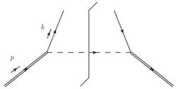
Figure 1: Lowest order contribution to $f^{\text{renorm,A}}_{q/p}(\xi;\mu)$.

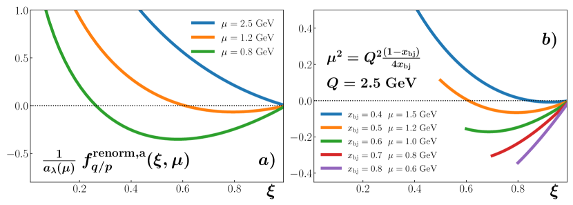
Figure 2: (a) An example of the $\overline{\rm MS}$ quark-in-proton pdf in Eq. (55) for several values of $\mu$, with $m_{q}=0.3$ GeV, $m_{p}=1.0$ GeV, and $m_{s}=1.5$ GeV. (b) Similar curves but in a form applicable to use in factorization for DIS with $\mu^{2}=\hat{s}/4$, given $Q=2.5~{}$GeV and several values for $x_{\rm bj}$. The pdfs are only used in the range $x_{\rm bj}\leq\xi\leq 1$, so the curves are restricted to this region.

We will work with the quark-in-proton pdf, for which the lowest order value is at order $a_{\lambda}$, from the graph in Fig. 1. A direct computation gives

$$f^{\text{renorm,A}}_{q/p}(\xi;\mu)$$

$$={} a_{\lambda}(\mu)(1-\xi)\left(\frac{(m_{q}+\xi m_{p})^{2}}{\Delta(\xi)}+\ln\left[\frac{\mu^{2}}{\Delta(\xi)}\right]-1\right)$$

$$+O\left(a_{\lambda}^{2}\right)\,,$$ (55)

where

$$\Delta(\xi)\equiv\xi m_{s}^{2}+(1-\xi)m_{q}^{2}-\xi(1-\xi)m_{p}^{2}\,.$$ (56)

(Note that $\Delta(\xi)$ is positive if the target state is stable, i.e., $m_{p}<m_{q}+m_{s}$.) The $\overline{\rm MS}$ counterterm used to obtain Eq. (55) is

$$\overline{\rm MS}\;\;\text{C.T.}=-a_{\lambda}(\mu)(1-\xi)\frac{S_{\epsilon}}{\epsilon}\,.$$ (57)

This gives $Z^{A}_{q/p}=-a_{\lambda}(\mu)(1-\xi)S_{\epsilon}/\epsilon+O(a_{\lambda}^{2})$, thereby matching the general form of Eq. (3).

By choosing $a_{\lambda}(\mu_{0})$ small enough at some reference scale $\mu_{0}$, we ensure that the one-loop renormalized pdf in Eq. (55) is a good approximation to the exact pdf to some given accuracy over a range of $\mu$. Since the effective coupling does not increase out of the perturbative range at small scales, unlike QCD, the calculation retains its accuracy when $\mu$ is of order particle masses. It only loses accuracy when $\mu$ is so large that the logarithms of $\mu/\mbox{mass}$ in higher orders of perturbation theory compensate the smallness of the coupling, and use of DGLAP evolution becomes necessary; that is not a concern here.

So that the results of calculations give suggestions as to what happens in QCD, we choose mass parameters to be in a range reminiscent of masses in QCD: $m_{q}=0.3$ GeV, $m_{p}=1.0$ GeV and $m_{s}=1.5$ GeV. Thus the quark mass is similar to the “constituent mass” [39] of a light quark in QCD, and similarly the hadron mass is similar to a nucleon mass. But we choose the diquark mass to be somewhat larger than might be expected were we to treat the calculation as an actual model for a pdf in non-perturbative QCD; this diquark mass allows us to illustrate that more than one mass scale could be relevant in a $\xi$-dependent way.

From Eq. (55), it immediately follows that for any given value of $\xi$, the pdf is negative for low enough $\mu$ and positive for large $\mu$. This is illustrated in Fig, 2(a) which shows the $\xi$-dependence of the quark pdf for three different values of $\mu$. The values are chosen to be representative of the low end of the range of $\mu$ used in QCD fits. At fairly low values of $\mu$, there is a range of moderately large $\xi$ where the pdf is negative. As $\mu$ increases, the range of negativity shrinks and eventually disappears. Later we will interpret these results in terms of scales in the shape of the transverse momentum distribution.

One might worry that the strong negativity might be incompatible with the momentum and flavor sum rules, which entail that some of the pdfs are sufficiently positive. This issue is resolved by observing that the nucleon in our Yukawa model is a possible parton, and that a first approximation to the corresponding pdf $f_{p/p}$ (diagonal in parton/particle labels) is the free-field value $\delta(\xi-1)$, which is positive, and does not involve any UV renormalization. Thus the quark-in-nucleon pdf that we have calculated is a minority contribution, i.e., much smaller than the other pdf at large $\xi$.

VIII.2 Systematics of why the pdf becomes negative

To understand how and where the $\overline{\rm MS}$ pdf becomes negative, we relate it to an integral over transverse momentum of the corresponding transverse momentum dependent (TMD) pdf. Calculating Eq. (55) involves calculating the following integral in dimensional regularization:

$$a_{\lambda}(\mu)\int_{0}^{\infty}\mathop{\mathrm{d}\mskip-0.59999muk^{2}_{\text{T}}}\nolimits k_{\text{T}}^{-2\epsilon}\frac{(1-\xi)\big{[}k_{\rm T}^{2}+(m_{q}+\xi m_{p})^{2}\big{]}}{\big{[}k_{\rm T}^{2}+\Delta(\xi)\big{]}^{2}}\,.$$ (58)

Suppose that instead of using dimensional regularization and subtracting the $\overline{\rm MS}$ pole to define a scale-dependent pdf, we simply applied a cutoff on transverse momentum in the unregulated integral:

$$a_{\lambda}(\mu)\int_{0}^{k^{2}_{\rm cut,\text{T}}}\mathop{\mathrm{d}\mskip-0.59999muk^{2}_{\text{T}}}\nolimits\frac{(1-\xi)\big{[}k_{\rm T}^{2}+(m_{q}+\xi m_{p})^{2}\big{]}}{\big{[}k_{\rm T}^{2}+\Delta(\xi)\big{]}^{2}}\,.$$ (59)

The new pdf is an ordinary integral with a positive integrand everywhere when $0<\xi<1$, with no further subtraction term. So, this pdf is guaranteed to be positive. It can be verified that when $k^{2}_{\rm cut,\text{T}}$ is set to equal $\mu^{2}$, the cut-off integral matches the $\overline{\rm MS}$ result in Eq. (55) except for corrections by a power of $m^{2}/\mu^{2}$, which are small at high scales. Its evolution is of the DGLAP form, but with a power-suppressed inhomogeneous term. In a gauge theory, there are problems with a naive use of a cutoff in transverse momentum, since the most natural definition of a TMD pdf suffers from rapidity divergences [33] associated with light-like Wilson lines. These necessitate changes in any method of working with TMD pdfs in QCD. But the same problem does not occur in a non-gauge theory.

Equation (59) is a very intuitive way to represent a scale-dependent pdf in terms of hadron structure: It contains the contributions from transverse momenta up to the cutoff. In particular, when $k^{2}_{\rm cut,\text{T}}$ is large, it includes, among other things, all the physics associated with intrinsic hadron structure. Then the coefficient function in factorization for DIS at high $Q$ can simply be characterized as whatever else contributes to the correct structure function. When $k^{2}_{\rm cut,\text{T}}$ is of order $Q^{2}$, the coefficient function is only concerned with physics at the scale $Q$.

Up to terms of order $m^{2}/k^{2}_{\rm cut,\text{T}}$, the pdf in Eq. (59) is related to the $\overline{\rm MS}$ pdf at scale $\mu$ by subtracting the term

$$a_{\lambda}(\mu)(1-\xi)\int_{\mu^{2}}^{k^{2}_{\rm cut,\text{T}}}\frac{\mathop{\mathrm{d}\mskip-0.59999muk^{2}_{\text{T}}}\nolimits}{{k^{2}_{\text{T}}}}\,,$$ (60)

as can be verified by explicit calculation. The integrand is the large $k_{\text{T}}$ asymptote of the integrand in Eq. (59), as is appropriate to the minimal subtraction used in the $\overline{\rm MS}$ scheme.

By taking $k^{2}_{\rm cut,\text{T}}$ to infinity, we find that the $\overline{\rm MS}$ pdf equals

$$a_{\lambda}(\mu)(1-\xi)\int_{0}^{\infty}\mathop{\mathrm{d}\mskip-0.59999muk^{2}_{\text{T}}}\nolimits\\ \left\{\frac{k_{\rm T}^{2}+(m_{q}+\xi m_{p})^{2}}{\big{[}k_{\rm T}^{2}+\Delta(\xi)\big{]}^{2}}-\frac{\theta(k_{\text{T}}-\mu)}{k_{\rm T}^{2}}\right\}\,,$$ (61)

i.e., there is a subtraction of the asymptote of the integrand, with a lower cutoff.

At high $k_{\text{T}}$, the subtraction term closely matches the first term. When $\mu$ is large, there is a logarithmic contribution from $k_{\text{T}}$ in the range $\Delta\lesssim k_{\text{T}}<\mu$, since the subtraction term vanishes there. The positive logarithmic contribution overwhelms any negativity in the remaining non-logarithmic contributions to the integral.

Now when $k_{\text{T}}$ goes to zero the $1/k^{2}_{\text{T}}$ term goes to infinity, unlike the first term in (61), giving a strong mismatch. Hence when $\mu$ is small, there is a large negative logarithmic contribution to the subtracted integral. Therefore, where the $\overline{\rm MS}$ pdf becomes negative is governed by the mass scale(s) below which the mismatch is strong.

When $\xi\to 0$, the first term in the integrand becomes $1/(k^{2}_{\text{T}}+m_{q}^{2})$. Then the pdf becomes negative when $\mu<m_{q}$, which is a low scale, well under a GeV.

When $\xi\to 1$, the term is

$$\frac{k_{\rm T}^{2}+(m_{q}+m_{p})^{2}}{(k_{\rm T}^{2}+m_{s}^{2})^{2}}\,.$$ (62)

Where the integral becomes negative is now governed by a combination of the scales $m_{q}+m_{p}$ and $m_{s}$, which are around a GeV or larger.

The existence of these two scales differing by a modest factor qualitatively explains Fig. 2. For $\mu$ in the middle of the range between the quark mass and about a GeV, the pdf is positive at low $\xi$ but not at high $\xi$. Only when $\mu$ is well above a GeV does the pdf become positive everywhere. The effect is enhanced by our choice of a somewhat large value of $m_{s}$, but it illustrates the effects of different scales of transverse momentum in different ranges of $\xi$ in a way that can easily happen in QCD. Indeed recent fits do provide results with negative values in some ranges of $\xi$ and $\mu$; we will discuss this below.

VIII.3 Relation to factorization

As to the impact of the negative values of pdfs on possibly predicting a negative cross section from a factorized form, we recall first that the factorized cross section is independent of $\mu$. But in finite order approximations, $\mu$-independence is valid only up to errors of the order of uncalculated higher order corrections. One should choose $\mu$ to avoid large logarithms in the perturbative expansion of the coefficient functions.

Furthermore, the factorization theorem itself is only valid up to errors of size $m_{q}^{2}/Q^{2}$, $m_{s}^{2}/Q^{2}$ and $m_{p}^{2}/Q^{2}$, with $x_{\rm bj}$-dependent coefficients. These arise from mismatches between the exact integrands for graphs for a structure function and the approximations used in obtaining the factorized form. Once the errors are too large compared with the factorized value of a cross section, negative values from the factorized cross section are irrelevant. In addition, when we work in QCD, the coupling becomes too large at low scales to allow low-order perturbative calculations of the coefficient functions to be useful.

In our model the second issue does not arise, and we examine the sizes of the power-law errors and their impact on the effect of negative pdfs, especially in relation to the mass scales involved. Because of our use of a weak coupling, it is sufficient to work at order $a_{\lambda}$. Some details of our calculations are given in Appendix A.

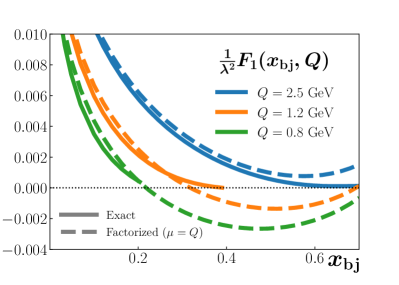
Figure 3: A comparison between Eq. (64) and the unfactorized graphs in Fig. 5 for the $F_{1}$ structure function (dropping $O\left(a_{\lambda}^{2}\right)$ terms), for three values of $Q$. The graphs are independent of the choice of $\mu$. The zero in the blue curve just above $x_{\rm bj}=0.5$ is the kinematical upper bound on Bjorken-$x_{\rm bj}$.

In Fig. 3, we compare an exact calculation of $F_{1}$ at order $a_{\lambda}$ with the factorized approximation, for three quite low values of $Q$. These are within the range of a number of experiments, e.g., Ref. [42]. The lowest value is $Q=0.8~{}$GeV, which is below where one normally uses factorization in QCD. But even there, there is a range of $x_{\rm bj}$, viz. $\lesssim 0.2$, where the factorized approximation is reasonably good. Recall that as $x_{\rm bj}$ gets small, the invariant mass of the final state gets large, so that the collision is quite inelastic and there is another larger scale in the problem than $Q$.

In contrast, at the larger $x_{\rm bj}$ values and fairly low $Q$, the factorized approximation is not merely a poor approximation, but in some places gives an unphysical negative value to $F_{1}$, while the true value is zero because the final state mass is below threshold.

As $Q$ increases, the range of $x_{\rm bj}$ where the factorized approximation is good increases, while the range of negative values for the approximation decreases. But the range of negative values does not closely match the range of negative values for the pdf. This is to be expected, since the calculation contains contributions from the one-loop coefficient function as well as directly from the negative pdf. At the highest value $Q=2.5~{}$GeV, the factorized approximation is positive everywhere. But at large $x_{\rm bj}$ it increases. Much of the increase is where the true value $F_{1}$ is zero because the final state is below the quark-diquark threshold, so that the factorized approximation is very incorrect.

From our calculation of the pdf in Sec. VIII.2, we saw that at small values of parton momentum fraction $\xi$, the width of the internal transverse momentum integration in the pdf is governed by the quark mass, which is $0.3~{}$GeV, a typical value for a constituent light quark mass, whereas at large $\xi$ the width is governed by the larger diquark mass. The approximation that leads to factorization involves neglecting quark transverse momentum in the hard scattering; in addition kinematic approximations involve neglecting $x_{\rm bj}m_{p}$ with respect to $Q$.

This suggests that at small enough $x_{\rm bj}$, the power error in factorization involves a relatively low mass, while at larger $x_{\rm bj}$ it involves a relatively high mass.

Now a standard choice of scale is $\mu=Q$. But, as observed in [3] for example, this is quite inappropriate at large $x_{\rm bj}$. The partonic transverse phase space is limited by $\hat{s}/4=Q^{2}(1-x_{\rm bj})/4x_{\rm bj}$, which produces large logarithms of $\hat{s}/Q^{2}$ at larger values of $x_{\rm bj}$ in the coefficient function. A consequence [3] is that choosing $\mu=Q$ gives considerable oversubtraction in the coefficient function. A more sensible value would be $\mu^{2}=\hat{s}/4$, at least at large $x_{\rm bj}$. For a given value of $Q$, this gets very small as $x_{\rm bj}\to 1$. Although this choice of $\mu$ should improve the perturbative treatment of hard parts, it substantially exacerbates the possibility that the value of a pdf in a calculation will turn negative, as illustrated in Fig. 2(b). This is the same as Fig. 2(a) but with $\mu^{2}=\hat{s}/4$ and a sequence of large values for $x_{\rm bj}$, with $Q^{2}=2$ GeV. But with such low values of the final state’s invariant mass, we must also expect that factorization also gives a poor approximation to the actual cross section.

Regardless of the details, we see that, given the mass scales $m_{p}$, $m_{q}$, and/or $m_{s}$, low values of $\mu$ result in a pdf that turns negative. The example is enough, therefore, to show that a pdf defined in the $\overline{\rm MS}$ scheme is not constrained by general principles to be positive everywhere. As mentioned in the Introduction, the result of calculations of heavy-quark pdfs provides one example of this phenomenon in QCD.

We have also seen that a negative pdf often occurs in a region of momentum fraction $\xi$ where power corrections cause factorization to be a poor approximation if $\xi=x_{\rm bj}$. Recall, however, that pdfs in the range $x_{\rm bj}\leq\xi\leq 1$ enter calculations at higher orders. So $\xi\sim 1$ pdfs are relevant even for small $x_{\rm bj}$ calculations.

VIII.4 “Bare” pdf of track B

We now find the corresponding bare pdf in track B. From the treatment in Sec. IV, we know that $f^{\text{bare,B}}$ is just Eq. (55), but before the $\overline{\rm MS}$ pole in Eq. (57) has been subtracted:

$$f^{\text{bare,B}}_{q/p}(\xi;\mu)=f^{\text{renorm,A}}_{\text{BPHZ}^{\prime}}$$

$$={} a_{\lambda}(\mu)(1-\xi)\left(\frac{(m_{q}+\xi m_{p})^{2}}{\Delta(\xi)}+\ln\left[\frac{\mu^{2}}{\Delta(\xi)}\right]-1\right)$$

$$+\left.a_{\lambda}(\mu)(1-\xi)\frac{S_{\epsilon}}{\epsilon}\right|_{\text{IR}}+O\left(a_{\lambda}^{2}\right)\,,$$ (63)

with terms of $O(\epsilon)$ ignored, and with the pole identified as collinear rather than UV. In the methods of track B, dimensional regularization is used to regulate collinear (and IR) divergences, so that $\epsilon<0$. Then the bare pdf in Eq. (63) is negative for small negative $\epsilon$.

IX Valence v. non-valence pdfs

The argument in the previous section about $\overline{\rm MS}$ pdfs becoming negative at small $\mu$ might appear to be quite general. It may seem that all pdfs should become entirely negative at small enough $\mu$ for all $\xi$. But this would be in contradiction with the sum rules obeyed by the pdfs, notably the momentum sum rule. These entail that the negativity at low $\mu$ cannot be a general property.

That worry is removed by observing that not all graphs for pdfs have UV divergences. In the model, the simplest case is for the nucleon-in-nucleon pdf, for which the lowest order value, including transverse momentum dependence is a simple delta function: $\delta(\xi-1)\delta^{(2)}(\boldsymbol{k}_{\text{T}}{})$; this obviously has no UV divergence when integrated over $\boldsymbol{k}_{\text{T}}{}$.

We characterize the situation by saying that in the model, the nucleon is itself the analog of a valence quark in QCD, while the quark in the model is an analog of a sea quark in QCD, given that the target particle is a nucleon. (For our rough purpose here, we characterize a valence quark, or, more generally, a valence parton as one that at large and moderately large momentum fraction corresponds at low scales to the largest pdfs and corresponds to the basic structure of the target state.)

The generalization to other theories, including QCD, can be explained by using the expansion (IV.1) of a pdf in terms of 2PI graphs. The part without a UV divergence is the first term in the expansion, i.e., the term without any rungs in the ladder. We notated it as $TB$. All the remaining terms in (IV.1) have UV divergences. Those statements follow from the standard power counting for UV divergences in pdfs. (Our Yukawa model provides a degenerate case where the lowest order 2PI graph is just a lowest order disconnected graph.)

The TB term is exactly the bare pdf $f^{\text{bare, CFP}}$ that was defined by Curci et al. [30]. This term is necessarily positive, by a version of the argument given in Sec. V.2, but without any complications arising due to the need for a regulator.

It is natural to suppose that $TB$ is dominated by the valence quark terms, which essentially correspond to simple quark models of hadrons. Any other terms, for non-valence partons, are presumably substantially smaller.

The argument leading to possible negative $\overline{\rm MS}$ pdfs applies to the graphs with rungs. We then get a two-component picture: A positive valence contribution from the TB term for the relevant pdfs, and then potentially negative contributions from the graphs with rungs. For non-valence partons, the first component is small, and so the potentially negative component from the renormalization of the UV divergent terms can dominate. Of course in QCD the coupling is not particularly small in the low $\mu$ region. So there is the potential for higher-order terms to modify the results.

As we observed, the negative contribution to a pdf goes away once $\mu$ is enough larger than the scale setting the width of the $\boldsymbol{k}_{\text{T}}{}$ distribution at small $\boldsymbol{k}_{\text{T}}{}$. But this is a soft constraint. As regards the potential for negative cross sections, the primary point is that negative values for pdfs arise in pdfs that are small compared with others, so higher-order perturbative terms in the hard scattering induced by valence quarks are not suppressed with respect to the lowest-order term induced by the minority partons.

Motivated by the calculations, a simple idea to see that some non-valence pdfs are likely to become negative at low enough scales is as follows. We examine consequences of DGLAP evolution: $df_{\rm min.}/d\ln\mu\simeq\text{kernel}\otimes f_{\rm maj}$. We first observe that at the lowest order those DGLAP kernels $P_{ij}(z,\alpha_{s})$ that are off-diagonal in parton flavor are positive. The diagonal kernels are positive when $z<1$, but have a negative delta-function at $z=1$. Suppose that at large $x$ we have a valence pdf, notably the $u$ quark in QCD, that is substantially larger than the others, and that is positive. Then the positivity of the off diagonal kernel implies that small pdfs increase with scale, but only for those partons with a non-zero LO DGLAP kernel with the valence parton. This is simply because a sufficient smallness of a pdf implies that the diagonal term in its evolution is smaller than the off-diagonal term.

Hence going to a lower scale takes such small pdfs to negative values. Direct examples of this are given not only by our model calculations, but also by the evolution of a heavy-quark pdf in QCD, when the scale $\mu$ is close to the heavy quark’s mass.

The increase with $\mu$ for a minority pdf contrasts with the well-known decrease of valence pdfs at the larger values of $x$. That decrease arises from the dominance of the delta-function terms in the DGLAP kernels that are diagonal in flavor. At sufficiently smaller $x$, the positive continuum part becomes more important and then the valence pdfs increase.

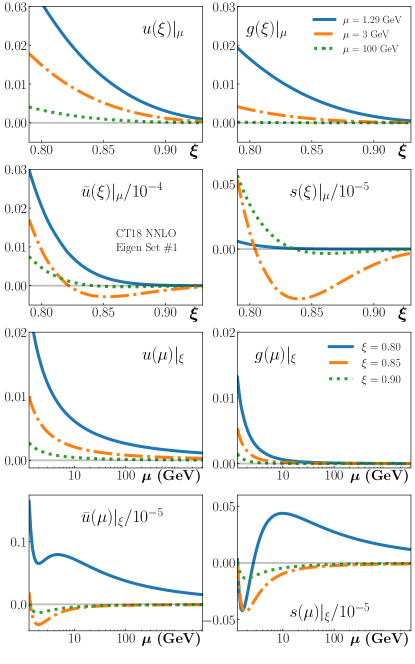
Figure 4: Pdfs from the CT18 fit [43] restricted to eigen-direction #1 at several values of scale as a function of $\xi$ (upper two rows) and at several large values of $\xi$ as a function of scale (lower two rows). To keep the number of plots lower, we have restricted the sea quark plots to $s$ and $\bar{u}$. Behavior of the $\bar{d}$ pdf is similar to that of the $\bar{u}$.

However, the expectations just summarized are somewhat in contrast with the results of actual fits, as illustrated in Fig. 4. In these plots we have focussed on $x$ above 0.8 using a particular eigen-direction pdf set from CT18 that displays negativity as an example. There is a clear hierarchy of sizes of pdf, with the pdf of the $u$ quark being the largest. We also notice that there are large discrepancies between the different fits for the pdfs of the sea quarks ($s$, $\bar{u}$) and of the gluon. This simply reflects the large uncertainties on these small pdfs in a region where they are weakly probed by the currently available data.

Moreover, the evolution for the minority pdfs, at scales of a GeV or two makes them decrease instead of increase with scale, initially. Some of the minority pdfs even stay negative up to $\mu\sim 100\,\textrm{GeV}$, which is not at all in agreement with the elementary prediction.

It is beyond the scope of this article to perform a detailed analysis. We make the following comments:

1. None of the other quarks has a lowest-order DGLAP kernel that connects it to the quark with the largest pdf, the $u$ quark. So the effect of the $u$ pdf on the evolution of the other quarks is indirect, both through an NLO kernel, and via the gluon pdf. Given the use of subtractions in defining the higher-order terms, the positivity properties are not at all clear compared with simple situations.

2. The coefficient functions in factorization, Eq. 7, have singularities at $x/\xi=1$, as do the DGLAP kernels. These generate large logarithms whenever pdfs are rapidly decreasing, as they are at large $\xi$. So fixed-order calculations of the kernels and of coefficient functions can be insufficient in this region. Then the errors due to omitted higher-order terms may not be small relative to lower-order terms, and large-$x$ resummation is needed to get accurate results. This was already observed by Candido et al. [3]; their argument for positivity of pdfs fails unless large-$x$ resummation is used. (That failure is beyond the other issues we discussed earlier.)

3. The negative pdfs are a few orders of magnitude below the largest pdf, of the $u$ quark. Thus the negativity has no direct consequences for negativity of cross sections.

4. They are also in a region where they are badly determined, and the uncertainty range [43] includes positive values. So one can always say that the negative values are not significant. The quoted values of pdfs in the unmeasured region are effectively extrapolations from regions where they are well measured.

5. Therefore there are liable to be implicit or explicit assumptions about the functional form of pdfs at their starting scale. For example, when an explicit parameterized form is used a restricted parameterization may be used which may not in reality be accurate enough at large $x$.

Another situation where negativity of pdfs is sometimes encountered is for gluons at small $x$ and fairly low $\mu$. There is a strong increase with scale of the gluon pdf, and depending on the size of the singlet and the gluon pdfs, reverse evolution to lower scales can give a negative gluon. However at small-$x$ there is loss of accuracy in fixed order calculations that requires small-$x$ resummation. For instance in [44] a global analysis with small-$x$ evolution was reported with the inferred gluon replicas being all positive in the small-$x$ in contrast to their baseline analysis based on fixed order calculations. As with the case of pdfs at large $x$, the possibly negative pdfs are in a region where they are weakly constrained by data.

X Conclusions

One of our main goals with this article has been to draw attention to gaps in one particularly common approach to QCD factorization. However, the issues are abstract and it is tempting to view them as only formal, with no impact on practical phenomenology. We have focused on the positivity question, therefore, to illustrate how those gaps can influence practical considerations. The positivity example shows that the track-A/track-B dichotomy is especially relevant to questions about the properties of the pdfs themselves. Other interesting examples likely exist.

Past approaches to pdf phenomenology have mainly focused on the universal nature of pdfs to constrain them from experimental scattering data. But increasingly sophisticated methods are being used to study pdfs and their properties directly using nonperturbative techniques like lattice QCD, and to combine those approaches with more traditional phenomenological approaches. It is important to check the derivation of properties that originally relied on a track-B view before they are adopted unchecked into larger phenomenological programs. More generally, the pitfalls of the track-B approach need to be taken into consideration in nonperturbative QCD approaches. Many of these calculations are performed at rather low scales where, as illustrated by the positivity example, the problems with track B are most prominent.

As regards the positivity issue itself, there are several points to make. First, we emphasize that we have not argued that $\overline{\rm MS}$ pdfs must be negative for any particular choice of scales or $\mu_{\overline{\rm MS}}$. Rather we proved that nothing in the definition of pdfs or in the factorization theorems themselves excludes negativity as a possibility, especially at low or moderate input scales. But we did show arguments that indicate that certain generic situations do tend to lead to negative pdfs of partons with small pdfs, notably for non-valence quarks. Giving a full theoretical answer to the question of whether a particular pdf turns negative depends on its large distance/low energy nonperturbative properties, as the sensitivity to mass scales in the example of Sec. VIII illustrates. Also, the failure of absolute positivity in the $\overline{\rm MS}$ scheme does not necessarily imply that other schemes do not exist which exactly preserve positivity.

Instead, we argue that imposing strict positivity on $\overline{\rm MS}$ pdfs as an absolute phenomenological constraint is an excessive theoretical bias. As our examples show, this is especially relevant to the question of how low $Q$ may be before factorization theorems become unreliable. Applications of factorization to low or moderate $Q$ are often important for studies of hadron structure. Note, for example, that past Jefferson Lab DIS measurements are in the range of $Q\sim m_{p}$ [45], with $Q>1$ GeV identified as the “canonical” DIS range. It is possible that for factorization theorems to continue to hold at these scales and with the desired precision, exact positivity constraints need to be relaxed. Indeed, if positivity constraints are relaxed, it is possible that DIS factorization theorems can be extended to significantly lower $Q$ than might otherwise be expected.

As we have seen, once the $\overline{\rm MS}$ scale $\mu$ is large enough compared with intrinsic transverse momentum scales, the pdfs indeed become positive.

Further refinements in knowledge about transverse momentum mass scales will likely help to sharpen estimates of where in kinematics a positivity assumption begins to be warranted. We leave such considerations to future work.

Given that positivity of pdfs is not absolutely guaranteed, there is the possibility that cross sections predicted by factorization can be negative. Indeed, we illustrated by calculation that a fixed-order factorized cross section can be unambiguously negative, without contradicting positivity of physical cross sections: A factorized cross section is only an approximation to the true cross section. If the difference between a measured and calculated cross section is within the expected error in factorization, then there is no contradiction. Two notable sources of error in particular kinematic regions are higher-order perturbative terms with logarithmic enhancements, and power corrections to factorization.

We conclude that positivity should not be imposed as an absolute constraint in fits for pdfs, neither on the pdfs nor on the calculated cross sections. Instead, any finding of a negative pdf or especially a negative cross section should be simply treated as a focus of attention. Does a negative pdf occur in a region where it can be expected? For a negative cross section, what are the expected errors and uncertainties? Which data are critical to obtaining the negative results?

Appendix A The full cross section

Since the $\overline{\rm MS}$ pdf only turns negative for rather low $\mu$, it is worthwhile to consider whether the scales must be so low that factorization theorems are badly violated. To test this, we can work out the exact, unfactorized lowest order cross section for deep inelastic scattering in the Yukawa theory of Sec. VIII and compare the results with the factorized expression that uses Eq. (55). The graphs contributing to the DIS cross section at lowest order and for $x_{\rm bj}<1$ are shown in Fig. 5. (The Hermitian conjugate of Fig. 5(c) is also needed, but for brevity we do not show it.)

The steps for deriving the factorization theorem [25] can be applied directly to these graphs. Namely, a sequence of approximations that neglect small, intrinsic mass scales relative to $Q$ lead (order-by-order in $a_{\lambda}$) to the separation into factors in Eq. (7). Errors are suppressed by powers of $\text{mass}^{2}/Q^{2}$. In the case of the $F_{1}$ structure function, the $\mathcal{C}$ becomes a partonic $\hat{F}_{1}$, and the quark-in-hadron pdf for the Yukawa theory is just the result in Eq. (55), while the lowest order hadron-in-hadron pdf is a $\delta$ function.

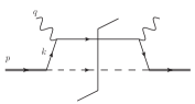
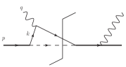
(a)	(b)	(c)

Figure 5: Contributions to DIS structure functions from Eq. (52) at $O\left(a_{\lambda}\right)$. Graph (a) is the “handbag” diagram that contributes at leading power and small transverse momentum. Graphs (b) and (c) contribute at leading power to large $k_{\text{T}}$. (the Hermitian conjugate for (c) is not shown).

The expression for the factorized $F_{1}$ structure function in DIS is

$${}F_{1}(x_{\rm bj},Q)\stackrel{{\scriptstyle x_{\rm bj}<1}}{{=}}\sum_{f}\int_{x_{\rm bj}}^{1}\frac{\mathop{\mathrm{d}\mskip-0.59999mu\xi}\nolimits{}}{\xi}\times$$

$$\times\frac{1}{2}\left\{\delta\left(1-\frac{x_{\rm bj}}{\xi}\right)\delta_{qf}+a_{\lambda}(\mu)\left(1-\frac{x_{\rm bj}}{\xi}\right)\left[\ln\left(4\right)-\frac{\left(\frac{x_{\rm bj}}{\xi}\right)^{2}-3\frac{x_{\rm bj}}{\xi}+\frac{3}{2}}{\left(1-\frac{x_{\rm bj}}{\xi}\right)^{2}}-\ln\frac{4x_{\rm bj}\mu^{2}}{Q^{2}(\xi-x_{\rm bj})}\right]\delta_{pf}\right\}\times$$

$${}\times\underbrace{\left\{\delta\left(1-\xi\right)\delta_{fp}+a_{\lambda}(\mu)(1-\xi)\left[\frac{(m_{q}+\xi m_{p})^{2}}{\Delta(\xi)}+\ln\left(\frac{\mu^{2}}{\Delta(\xi)}\right)-1\right]\delta_{fq}\right\}}_{f_{f/p}(\xi;\mu)}$$

$${}\qquad+O\left(a_{\lambda}(\mu)^{2}\right)+O\left(m^{2}/Q^{2}\right)\,.$$ (64)

Both the hadron-in-hadron pdf and the order-$a_{\lambda}$ quark-in-hadron pdf appear in the braces on the third line. Note that the $\mu$-dependence cancels between the second and third lines up to order $a_{\lambda}^{2}$, as expected. The expression for the unfactorized structure function is straightforward but rather complex and so we do not display it here.

Using the same numerical values for parameters as were used in Fig. 2, we compare Eq. (64) (dropping both the $O\left(a_{\lambda}^{2}\right)$ terms and the $O\left(m^{2}/Q^{2}\right)$ terms) with the exact $O\left(a_{\lambda}\right)$ $F_{1}$ in Fig. 3 for several values of $Q$.

References

- Diehl and Stienemeier [2020] M. Diehl and P. Stienemeier, Gluons and sea quarks in the proton at low scales, Eur. Phys. J. Plus 135, 211 (2020), arXiv:1904.10722 [hep-ph] .
- Martin et al. [2009] A. Martin, W. Stirling, R. Thorne, and G. Watt, Parton distributions for the LHC, Eur. Phys. J. C63, 189 (2009), arXiv:0901.0002 [hep-ph] .
- Candido et al. [2020] A. Candido, S. Forte, and F. Hekhorn, Can parton distributions be negative?, JHEP 11, 129, arXiv:2006.07377 [hep-ph] .
- Feynman [1972] R. P. Feynman, Photon-Hadron Interactions (Benjamin, Reading, MA, 1972).
- Soffer [1995] J. Soffer, Positivity constraints for spin dependent parton distributions, Phys. Rev. Lett. 74, 1292 (1995), arXiv:hep-ph/9409254 .
- Goldstein et al. [1995] G. R. Goldstein, R. Jaffe, and X.-D. Ji, Soffer’s inequality, Phys. Rev. D 52, 5006 (1995), arXiv:hep-ph/9501297 .
- Barone [1997] V. Barone, On the QCD evolution of the transversity distribution, Phys. Lett. B 409, 499 (1997), arXiv:hep-ph/9703343 .
- Ji [2013] X. Ji, Parton Physics on a Euclidean Lattice, Phys. Rev. Lett. 110, 262002 (2013), arXiv:1305.1539 [hep-ph] .
- Xiong et al. [2014] X. Xiong, X. Ji, J.-H. Zhang, and Y. Zhao, One-loop matching for parton distributions: Nonsinglet case, Phys. Rev. D 90, 014051 (2014), arXiv:1310.7471 [hep-ph] .
- Ma and Qiu [2018] Y.-Q. Ma and J.-W. Qiu, Extracting Parton Distribution Functions from Lattice QCD Calculations, Phys. Rev. D 98, 074021 (2018), arXiv:1404.6860 [hep-ph] .
- Constantinou [2021] M. Constantinou, The -dependence of hadronic parton distributions: A review on the progress of lattice QCD, Eur. Phys. J. A 57, 77 (2021), arXiv:2010.02445 [hep-lat] .
- Bhat et al. [2021] M. Bhat, K. Cichy, M. Constantinou, and A. Scapellato, Flavor nonsinglet parton distribution functions from lattice QCD at physical quark masses via the pseudodistribution approach, Phys. Rev. D 103, 034510 (2021), arXiv:2005.02102 [hep-lat] .
- Joó et al. [2019] B. Joó, J. Karpie, K. Orginos, A. Radyushkin, D. Richards, and S. Zafeiropoulos, Parton Distribution Functions from Ioffe time pseudo-distributions, JHEP 12, 081, arXiv:1908.09771 [hep-lat] .
- Bednar et al. [2020] K. D. Bednar, I. C. Cloët, and P. C. Tandy, Distinguishing Quarks and Gluons in Pion and Kaon Parton Distribution Functions, Phys. Rev. Lett. 124, 042002 (2020), arXiv:1811.12310 [nucl-th] .
- Thorne [2006] R. Thorne, A Variable-flavor number scheme for next-to-next-to-leading order, Phys. Rev. D 73, 054019 (2006), arXiv:hep-ph/0601245 .
- Buza et al. [1998] M. Buza, Y. Matiounine, J. Smith, and W. L. van Neerven, Charm electroproduction viewed in the variable flavor number scheme versus fixed order perturbation theory, Eur. Phys. J. C 1, 301 (1998), arXiv:hep-ph/9612398 .
- Kogut and Soper [1970] J. B. Kogut and D. E. Soper, Quantum electrodynamics in the infinite momentum frame, Phys. Rev. D1, 2901 (1970).
- Bouchiat et al. [1971] C. Bouchiat, P. Fayet, and P. Meyer, Galilean invariance in the infinite momentum frame and the parton model, Nucl. Phys. B34, 157 (1971).
- Soper [1977] D. E. Soper, The Parton Model and the Bethe-Salpeter Wave Function, Phys. Rev. D 15, 1141 (1977).
- Soper [1979] D. E. Soper, Partons and their transverse momenta in QCD, Phys. Rev. Lett. 43, 1847 (1979).
- Collins [1980] J. C. Collins, Intrinsic transverse momentum. Nongauge theories, Phys. Rev. D 21, 2962 (1980).
- Collins and Soper [1982] J. C. Collins and D. E. Soper, Parton distribution and decay functions, Nucl. Phys. B194, 445 (1982).
- Wilson [1969] K. G. Wilson, Nonlagrangian models of current algebra, Phys. Rev. 179, 1499 (1969).
- Zimmermann [1973] W. Zimmermann, Normal products and the short distance expansion in the perturbation theory of renormalizable interactions, Ann. Phys. 77, 570 (1973).
- Collins [2011] J. C. Collins, Foundations of Perturbative QCD (Cambridge University Press, Cambridge, 2011).
- Chetyrkin and Tkachov [1982] K. G. Chetyrkin and F. V. Tkachov, Infrared -operation and ultraviolet counterterms in the MS scheme, Phys. Lett. B 114, 340 (1982).
- Chetyrkin and Smirnov [1984] K. G. Chetyrkin and V. A. Smirnov, -Operation corrected, Phys. Lett. B 144, 419 (1984).
- Smirnov and Chetyrkin [1985] V. A. Smirnov and K. G. Chetyrkin, operation in the minimal subtraction scheme, Theor. Math. Phys. 63, 462 (1985).
- Ellis et al. [1979] R. K. Ellis, H. Georgi, M. Machacek, H. D. Politzer, and G. G. Ross, Perturbation theory and the parton model in QCD, Nucl. Phys. B152, 285 (1979).
- Curci et al. [1980] G. Curci, W. Furmanski, and R. Petronzio, Evolution of parton densities beyond leading order: The nonsinglet case, Nucl. Phys. B175, 27 (1980).
- Politzer [1977] H. Politzer, Gluon Corrections to Drell-Yan Processes, Nucl. Phys. B 129, 301 (1977).
- Collins [1998] J. C. Collins, Hard-scattering factorization with heavy quarks: A general treatment, Phys. Rev. D58, 094002 (1998), hep-ph/9806259 .
- Collins [2003] J. C. Collins, What exactly is a parton density?, Acta Phys. Polon. B34, 3103 (2003), hep-ph/0304122 .
- Valatin [1954a] J. Valatin, Singularities of electron kernel functions in an external electromagnetic field, Proc. Roy. Soc. A 222, 93 (1954a).
- Valatin [1954b] J. Valatin, On the Dirac-Heisenberg theory of vacuum polarization, Proc. Roy. Soc. A 222, 228 (1954b).
- Valatin [1954c] J. Valatin, On the propagation functions of quantum electrodynamics, Proc. Roy. Soc. A 225, 535 (1954c).
- Valatin [1954d] J. Valatin, On the definition of finite operator quantities in quantum electrodynamics, Proc. Roy. Soc. A 226, 254 (1954d).
- Wilson [1973] K. G. Wilson, Quantum field theory models in less than 4 dimensions, Phys. Rev. D7, 2911 (1973).
- De Rújula et al. [1975] A. De Rújula, H. Georgi, and S. L. Glashow, Hadron Masses in a Gauge Theory, Phys. Rev. D 12, 147 (1975).
- Lepage and Brodsky [1980] G. P. Lepage and S. J. Brodsky, Exclusive processes in perturbative quantum chromodynamics, Phys. Rev. D22, 2157 (1980).
- Brodsky et al. [2001] S. J. Brodsky, D.-S. Hwang, B.-Q. Ma, and I. Schmidt, Light-cone representation of the spin and orbital angular momentum of relativistic composite systems, Nucl. Phys. B593, 311 (2001), hep-th/0003082 .
- Adolph et al. [2013] C. Adolph et al. (COMPASS), Hadron Transverse Momentum Distributions in Muon Deep Inelastic Scattering at 160 GeV/, Eur. Phys. J. C 73, 2531 (2013), [Erratum: Eur.Phys.J.C 75, 94 (2015)], arXiv:1305.7317 [hep-ex] .
- Hou et al. [2021] T.-J. Hou et al., New CTEQ global analysis of quantum chromodynamics with high-precision data from the LHC, Phys. Rev. D 103, 014013 (2021), arXiv:1912.10053 [hep-ph] .
- Ball et al. [2018] R. D. Ball, V. Bertone, M. Bonvini, S. Marzani, J. Rojo, and L. Rottoli, Parton distributions with small-x resummation: evidence for BFKL dynamics in HERA data, Eur. Phys. J. C 78, 321 (2018), arXiv:1710.05935 [hep-ph] .
- Gaskell [2010] D. Gaskell, Recent results in DIS from Jefferson Lab, PoS DIS12010, 009 (2010).