Triple crossing positivity bounds for multi-field​ theories

Abstract

We develop a formalism to extract triple crossing symmetric positivity bounds for effective field theories with multiple degrees of freedom, by making use of $su$ symmetric dispersion relations supplemented with positivity of the partial waves, $st$ null constraints and the generalized optical theorem. This generalizes the convex cone approach to constrain the $s^{2}$ coefficient space to higher orders. Optimal positive bounds can be extracted by semi-definite programs with a continuous decision variable, compared with linear programs for the case of a single field. As an example, we explicitly compute the positivity constraints on bi-scalar theories, and find all the Wilson coefficients can be constrained in a finite region, including the coefficients with odd powers of $s$, which are absent in the single scalar case.

1 Introduction and summary

Recently, there has been significant progress in understanding the consistent parameter spaces of effective field theories (EFTs) in the form of positivity bounds. These are constraints on the Wilson coefficients of an EFT, or more generally on some physical observables derived from the EFT scattering amplitudes, and arise from simply assuming the EFT’s UV completion is consistent with fundamental principles of S-matrix such as causality/analyticity and unitarity. The positivity bounds can be quite stringent, often eliminating large chunks of the naive parameter space, which highlights the fact that not everything consistent with the symmetries can be a valid EFT.

Applying the optical theorem to the dispersion relation for an identical scalar amplitude, one can derive the forward positivity bound which states that the Wilson coefficient in front of $s^{2}$ should be positive Adams:2006sv (see also earlier works Pham:1985cr ; Ananthanarayan:1994hf ), $s,t,u$ being the standard Mandelstam variables. There are a few directions to generalize the scope and strength of positivity bounds for 2-to-2 scattering. First of all, the same argument for the $s^{2}$ bound can also be used to infer that the coefficients in front of all even powers of $s$ are all positive, if the theory is weakly coupled at least in the IR. But there is more to the forward dispersion relation than meets the eye of the optical theorem’s positivity. In fact, the Hankel matrix of all the coefficients of even $s$ powers are also positive definite Arkani-Hamed:2020blm , as can be seen from the connection to the (mathematical) moment problems Arkani-Hamed:2020blm ; Bellazzini:2020cot . Once the $t$ expansion of the dispersion relation is also included, the structure of positivity bounds becomes much richer. By using the positivity of derivatives of the amplitude’s absorptive part and relaxing the UV scale of the dispersive integrand, Ref deRham:2017avq derived an infinite tower of positivity bounds away from the forward limit that can be cast as a recurrence relation involving $s$ and $t$ derivatives (see Manohar:2008tc ; Nicolis:2009qm ; Bellazzini:2016xrt for earlier works on going beyond the forward limit). These recurrence bounds have also been generalized to massive particles with spin using the transversity basis for the external polarizations in which $su$ crossing relations are (semi-)diagonalized deRham:2017zjm .

However, these recurrence positivity bounds only utilized the $su$ crossing symmetry that is inherent in the twice subtracted dispersion relation. It has been realized that huge gains can be profited if one imposes $st$ crossing symmetry on the $su$ symmetric dispersion relation, which allows us to bound all the coefficients in the $s,t$ expansion both from above and below Tolley:2020gtv ; Caron-Huot:2020cmc . Specifically, the $st$ crossing symmetry implies that certain linear combinations of the Wilson coefficients in the $su$ symmetric expansion of the EFT amplitude have to vanish, which, by substituting in the sum rules from the $su$ symmetric dispersion relation, gives rise to an infinite series of null constraints on the dispersive integrals. These null constraints can be added into the sum rules of the Wilson coefficients to form linear programs to extract the optimal bounds from the positivity of the UV spectral function. These linear programs involve a continuous decision variable, which nevertheless can be efficiently solved by the publicly available SDPB package Simmons-Duffin:2015qma . For the $s^{2}$ coefficient, Ref Caron-Huot:2020cmc was also able to derive an upper bound in terms of the cutoff, thanks to the upper bound of partial wave unitarity and the first null constraint. For the case of a single scalar field, these new triple crossing symmetric bounds can restrict the dimensionless Wilson coefficients to be parametrically order $\mathcal{O}(1)$. This is of course something one naturally expects, as can be seen in many examples by explicitly integrating out the heavy fields from the UV models, but these new bounds put the naturalness argument on a rigorous and concrete footing, barring the possibility of a potential accidental large coupling.

An alternative way to use the triple permutation symmetry of a scalar amplitude is to start with a dispersion relation that is triple symmetric Sinha:2020win (based on an earlier work Auberson:1972prg ), and then locality enforces an alternative set of null constraints on the triple symmetric dispersion relation. Yet, another way to extract the same positivity bounds Chiang:2021ziz is to first perform a general linear rotation to simplify the partial wave expansion in the dispersion relation and then convert the problem to a bi-variate moment problem that is well studied in mathematics. Whether a point in the parameter space satisfies the positivity bounds can then be determined by checking positive definiteness of a series of coefficient matrices, and the null constraints in this way can be imposed at the level of Wilson coefficients, that is, by slicing out the triple crossing symmetric subspace of the allowed bounds.

An interesting application of these triple crossing symmetric bounds is that, while the forward positivity bound can marginally rule out Adams:2006sv massless Galileon theory Nicolis:2008in , which arises as decoupling limits of several gravitational models (see e.g., deRham:2016nuf ), the new bounds can now effectively rule out Galileon theories where the Galileon symmetry is weakly broken, as these bounds dictate that the weakly broken scale must be parametrically close to the cutoff scale in these theories Tolley:2020gtv . On the other hand, full-blown applications of positivity bounds in gravitational theories requires a judicial treatment of the $t$ channel pole, which survives the twice subtraction and whose singularity in the forward limit is balanced out by the divergence in the dispersive integral. By transforming to the impact parameter space, it has been shown that the forward singularity can be overcome, carving out some sharp boundaries for the swampland Caron-Huot:2021rmr . See Bellazzini:2015cra ; Cheung:2016yqr ; Bonifacio:2016wcb ; deRham:2017imi ; Bellazzini:2017fep ; deRham:2018qqo ; Bonifacio:2018vzv ; Melville:2019wyy ; deRham:2019ctd ; Alberte:2019xfh ; Alberte:2020bdz ; Chen:2019qvr ; Huang:2020nqy ; Alberte:2020jsk ; Tokuda:2020mlf ; Wang:2020xlt ; Herrero-Valea:2019hde ; Herrero-Valea:2020wxz ; deRham:2021fpu ; Traykova:2021hbr ; Bern:2021ppb ; Arkani-Hamed:2021ajd ; Davis:2021oce for some other interesting discussions of positivity bounds in gravity and cosmology.

While the above positivity bounds for a single scalar field presents a significant step towards a better understanding of the structure of the parameter space of EFTs, our universe is more complex than just a single scalar field. We typically encounter EFTs with many degrees of freedom. In the absence of any new particle signals at the LHC, the EFT approach to parameterize possible Beyond the Standard Model physics has become increasingly popular. In the Standard Model EFT (SMEFT), for example, there are a large number of low energy modes. How to optimally handle many degrees of freedom adds a whole new dimension to the problem of extracting the positivity bounds in a generic EFT. Recently, progress has been made in this direction for the lowest order $s^{2}$ coefficients, the positivity bounds on which are of course important phenomenologically.

If there are many modes in a low energy EFT, a simple generalization of the elastic positivity bounds is to linearly superpose the different modes to get elastic positivity bounds for the superposed states. However, this does not produce the strongest positivity bounds, as it misses positivity bounds coming from considering elastic amplitudes between “entangled states” Zhang:2020jyn ; Li:2021lpe . By using generalized optical theorem, one can see that the $s^{2}$ coefficients of the multi-field amplitudes form a convex cone, whose extremal rays correspond to irreps of the EFT symmetries or one particle UV states projected down to the EFT symmetries Zhang:2020jyn . This highlights the importance of positivity bounds in inverse-engineering the UV completion of SMEFT and the importance of higher order operators in Beyond the Standard Model phenomenology. Furthermore, the dual of the amplitude cone is a spectrahedron, and thus finding the strongest positivity bounds can be turned into a (normal) semi-definite program (SDP) Li:2021lpe , which can be efficiently solved by many widely available algorithms. Other applications of positivity bounds in SMEFT can be found in Zhang:2018shp ; Bi:2019phv ; Yamashita:2020gtt ; Fuks:2020ujk ; Zhang:2020jyn ; Gu:2020ldn ; Li:2021lpe ; Vecchi:2007na ; Bellazzini:2018paj ; Remmen:2019cyz ; Trott:2020ebl ; Remmen:2020vts ; Bonnefoy:2020yee ; Chala:2021wpj . Also, see Distler:2006if ; Remmen:2020uze ; Grall:2021xxm ; Davighi:2021osh ; Haldar:2021rri ; Raman:2021pkf ; Gopakumar:2021dvg ; Zahed:2021ffy ; Kundu:2021qpi for a few other generalizations of positivity bounds, and Paulos:2016fap ; Guerrieri:2020bto ; Hebbar:2020ukp ; Guerrieri:2021tak and reference therein for recent progress in S-matrix bootstrap, which overlaps the development of positivity bounds.

In this paper, we initiate the study of positivity bounds on higher order Wilson coefficients for theories with multiple degrees of freedom, incorporating both the triple crossing and convex cone approach, to better the understanding of the parameter space structure of multi-field EFTs. We will focus on theories with scalar fields only, which have simpler partial wave expansions. For the multi-field case, the dispersion relation contains a spectral tensor that is indexed by the four external particles and is not necessarily positive for generic combinations of the particles. To extract the optimal bounds, we take a convex geometry approach to view this spectral tensor as living in a convex cone. A key observation is that the dual cone of the spectral tensor cone is a spectrahedron. This allows us to formulate an SDP with only one continuous decision variable to extract the optimal positivity bounds, which can again be efficiently solved by the SDPB package. This is compared to the single scalar case which can be formulated as linear programs with one continuous variable. For both cases, the continuous variable comes from the dispersive integral and is associated with possible scales of the UV states. On the other hand, this is also similar to the $s^{2}$ convex cone, but now the spectrahedron depends on the partial waves, the UV scale and the orders of the $v=s+t/2$ and $t$ expansion.

Due to the multi-field structure, the generic $st$ null constraints are now more complex, as they are now indexed by the external particles and the external particle indices are swapped for some terms in the constraints. Nevertheless, a convenient way to add them to the SDP is essentially to invoke something similar to the dual cone for the Wilson coefficients. As the null constraints are equalities, instead of inequalities that are used to define the dual cone in convex geometry, the structure that is introduced is really just the boundary of the dual cone. Another way to use our formalism, which is not explicitly demonstrated in the paper, is to perform the SDPs without adding the dispersive null constraints. Instead, the null constraints are to be imposed as equalities on the Wilson coefficients directly. That is, one restricts the outcomes of these SDPs to the subspace defined by the null constraints in the coefficient space. However, this typically involves computing SDPs with quite a few coefficients, as even the lowest null constraints in a multi-field theory already contain quite a few coefficients. If we are faced with a problem that involves only a couple of particular coefficients, the approach explicitly implemented in this paper is much more efficient.

We also generalize the upper bounds of the $v^{2}$ coefficients, which can be again implemented by supplementing the spectral tensor with a dual structure. The $v^{2}$ coefficients can be constrained to be in a finite region by combining the $v^{2}$ cone bounds and these generalized upper bounds, which as we shall see is essential to bound all the coefficients in a multi-field EFT to an enclosed region.

As an illustration, we apply the formalism to constrain the Wilson coefficients of bi-scalar theories endowed with some discrete symmetries. We explore the geometric shapes for the $v^{2}$ and $v^{2}t$ coefficients and also compute two-sided bounds for higher order coefficients, which are obtained agnostic about the other coefficients. To obtain these two-sided bounds, it is essential to take into account the finiteness of the $v^{2}$ coefficients. Different from the single scalar case, we now also have coefficients with odd powers of $s$, and we find that these coefficients are also bounded from both sides, despite that its associated (raw) spectral tensor does not form a salient cone. All in all, the triple crossing bounds can be used to constrain the Wilson coefficients of a multi-field EFT in a finite region near the origin.

The paper is organized as follows. In Section 2, we derive the $su$ symmetric dispersion relation and expand the relation to get sum rules for all the Wilson coefficients, and then we impose $st$ crossing symmetry to get the null constraints on the dispersion relation. In Section 3, we formulate the extraction of triple crossing symmetric positivity bounds as SDPs, show how these programs can be implemented with SDPB, and generalize the $v^{2}$ upper bound to the multi-field case. In Section 4, for a simple example, we explicitly calculate the triple crossing positivity bounds for bi-scalar theory with the double $\mathbb{Z}_{2}$ symmetry and the $\mathbb{Z}_{2}$ symmetry, with the numerical results presented in five figures and one table. In Appendix A, we list the explicit expressions for a few quantities used in the first few null constraints for a quick reference. A briefly discussion on generalization to the case with massive fields is presented in Appendix B.

2 Sum rules for multi-fields

In many circumstances, EFTs contain multiple low energy modes in their spectrum so as to reproduce our phenomenal world. Let us suppose that there are $N$ light modes in a $D$ dimensional low energy EFT. Consider an EFT with a large hierarchy between the cutoff and the masses of the modes, $\Lambda\gg m_{i}$, so that it is a good approximation to take the massless limit $m_{i}\to 0$, and therefore we have the following simple kinematic relations

$$s+t+u=0,\leavevmode\nobreak\ \leavevmode\nobreak\ \leavevmode\nobreak\ \cos\theta=1+\frac{2t}{s},$$ (1)

where $s=-(p_{1}+p_{2})^{2},t=-(p_{1}-p_{3})^{2},u=-(p_{1}-p_{4})^{2}$ with $p_{1},p_{2},p_{3},p_{4}$ being the external momenta, and $\theta$ is the scattering angle between particle 1 and 3. For simplicity, we will consider multi-scalar theories as our examples, as their partial wave expansion is easier to perform explicitly. For massive scalars, whose crossing relations are still trivial, a generalization to the case with the same mass is also straightforward — see Appendix B. We will assume that the EFT is weakly coupled and loop contributions are suppressed below the cutoff, so we can focus on the leading tree level amplitudes. For tree level amplitudes, the positivity bounds can be directly expressed in terms of the Wilson coefficients, while for the loop amplitudes it might be more convenient to express the bounds in terms of observables derived from the amplitude.

2.1 $su$ symmetric dispersion relation

To derive positivity bounds for an EFT, we make use of the $su$ symmetric dispersion relation, whose existence reflects unitarity, analyticity, locality and crossing symmetry of the underlying UV amplitude. Consider UV scattering amplitude $A_{ijkl}(s,t)$ for process $ij\to kl$, where $i,j,k,l=1,2,...,N$ label different low energy modes. Following the same steps as the case of a single scalar (see, eg, deRham:2017avq ), particularly utilizing Cauchy’s integral formula for $A_{ijkl}(s,t)$ in the complex $s$ plane for fixed $t$ along with the Froissart-Martin bound Froissart:1961ux ; Martin:1962rt and $su$ crossing symmetry, we can express the amplitude as a dispersive integral of the absorptive part of the amplitude over $\mu>\Lambda^{2}$:

$$B_{ijkl}(s,t) \equiv A_{ijkl}(s,t)-\frac{{\lambda}_{ijkl}}{-s}-\frac{{\lambda}_{ijkl}}{-t}-\frac{{\lambda}_{ijkl}}{-u}$$ (2)

$$=a^{(0)}_{ijkl}(t)+a^{(1)}_{ijkl}(t)s+\int^{\infty}_{\Lambda^{2}}\frac{\mathrm{d}\mu}{\pi(\mu-\mu_{p})^{2}}\left[\frac{(s-\mu_{p})^{2}}{\mu-s}{\rm Abs}\,A_{ijkl}(\mu,t)+\frac{(u-\mu_{p})^{2}}{\mu-u}{\rm Abs}\,A_{ilkj}(\mu,t)\right]$$

$$=a^{(0)}_{ijkl}(t)+a^{(1)}_{ijkl}(t)s+\int^{\infty}_{\Lambda^{2}}\frac{\mathrm{d}\mu}{\pi(\mu+\frac{t}{2})^{2}}\left[\frac{(s+\frac{t}{2})^{2}}{\mu-s}{\rm Abs}\,A_{ijkl}(\mu,t)+\frac{(u+\frac{t}{2})^{2}}{\mu-u}{\rm Abs}\,A_{ilkj}(\mu,t)\right],$$

where $\Lambda$ is the scale at which the lowest heavy modes come in, identified with the cutoff here for simplicity and the absorptive part is defined as ${\rm Abs}\,A(\mu,t)=\frac{1}{2i}{\rm Disc}\,A(\mu,t)=\frac{1}{2i}\big{[}A(\mu+i\epsilon,t)-A(\mu-i\epsilon,t)\big{]}$ with $\epsilon\to 0^{+}$. When $A_{ijkl}$ is time reversal invariant, the absorptive part reduces to the imaginary part ${\rm Abs}\,A_{ijkl}(\mu,t)={\rm Im}A_{ijkl}(\mu,t)$. This is the so-called twice subtracted dispersion relation with the subtraction terms $a^{(0)}_{ijkl}(t)$ and $a^{(1)}_{ijkl}(t)$, which are needed because the Froissart-Martin bound, derived from unitarity, analyticity and locality/polynomial boundedness, can only constrain the UV behavior of ${\rm Abs}\,A_{ilkj}(s,t)$ to diverge slower than $s^{2}$. In the last line of the equation above, we have chosen the subtraction point at $\mu_{p}=-{t}/2$ so that $(s+\frac{t}{2})^{2}=(u+\frac{t}{2})^{2}$ can factor out of the whole dispersive integral, which allows us to define a convenient SDP later. Since $B_{ijkl}(s,t)$ is $su$ symmetric, we have $B_{ijkl}(s,t)=B_{ilkj}(u,t)$, so $a^{(0)}_{ijkl}(t)$ and $a^{(1)}_{ijkl}(t)$ must satisfy the following relations

$$a^{(1)}_{ijkl}(t)=-a^{(1)}_{ilkj}(t),\leavevmode\nobreak\ \leavevmode\nobreak\ \leavevmode\nobreak\ \leavevmode\nobreak\ a^{(0)}_{ijkl}(t)=a^{(0)}_{ilkj}(t)-a^{(1)}_{ilkj}(t)t.$$ (3)

We have chosen the scalar fields to be in a self-conjugate basis for simplicity, but the formalism below can be easily generalized for a general basis, in which one should additionally conjugate the particle after crossing. For example, the crossing symmetry would be $B_{ijkl}(s,t)=B_{i\bar{l}k\bar{j}}(u,t)$ and the $u$ channel part of the dispersion relation would have ${\rm Abs}\,A_{i\bar{l}k\bar{j}}(\mu,t)$, where $\bar{j}$ and $\bar{l}$ stands for the conjugate particle of $j$ and $l$ respectively.

For our later convenience, it is useful to introduce a new momentum invariant $v$ to replace the $s$ variable

$$v=s+\frac{t}{2},$$ (4)

and then the $s\leftrightarrow u$ crossing symmetry simply becomes $v\leftrightarrow-v$:

$$B_{ijkl}(s,t)=B_{ilkj}(u,t)\leavevmode\nobreak\ \leavevmode\nobreak\ \Longrightarrow\leavevmode\nobreak\ \leavevmode\nobreak\ \tilde{B}_{ijkl}\left(v,t\right)=\tilde{B}_{ilkj}\left(-v,t\right),$$ (5)

where we have defined $\tilde{B}_{ijkl}(v,t)\equiv B_{ijkl}(s,t)$. Then we can write the dispersion relation as

$$\tilde{B}_{ijkl}(v,t)=\tilde{a}^{(0)}_{ijkl}(t)+a^{(1)}_{ijkl}(t)v+v^{2}\int^{\infty}_{\Lambda^{2}}\frac{\mathrm{d}\mu}{\pi(\mu+\frac{t}{2})^{2}}\left[\frac{{\rm Abs}\,A_{ijkl}(\mu,t)}{\mu+\frac{t}{2}-v}+\frac{{\rm Abs}\,A_{ilkj}(\mu,t)}{\mu+\frac{t}{2}+v}\right].$$ (6)

For elastic scattering, i.e., when $i=k,\leavevmode\nobreak\ j=l$, we can also factor out ${\rm Abs}\,A_{ijij}(\mu,t)$ in the integrand and have $a^{(1)}_{ijij}(t)=-a^{(1)}_{ijij}(t)=0$, which means that there will be only even powers of $v$ on the both sides of the dispersion relation, as is the case for scattering between identical particles. For inelastic scattering amplitudes, odd powers of $v$ are generally present, and we will see that the Wilson coefficients of these terms also have two-sided bounds, despite their individual spectral tensors not forming salient cones. The remarkable feature of the dispersion relation is that on the left hand side the quantity $B_{ijkl}(s,t)$ can be well approximated by the EFT computations for $s,t\ll\Lambda^{2}$, while the right hand side relies on the absorptive part of the amplitude from the high energy UV theory, noting that the integration goes all the way up to infinity. In other words, the dispersion relation is a tool for us to use some salient properties of UV physics to constrain the EFT in the IR.

The absorptive part of the amplitude can be expanded by partial waves

$${\rm Abs}\,A_{ijkl}(\mu,t)=\frac{2^{4{\alpha}+2}\pi^{\alpha}\Gamma({\alpha})}{\mu^{{\alpha}-\frac{1}{2}}}\sum_{\ell=0}^{\infty}(2\ell+2{\alpha})C^{({\alpha})}_{\ell}\left(1+\frac{2t}{\mu}\right){\rm Abs}\,a^{ijkl}_{\ell}(\mu),\leavevmode\nobreak\ \leavevmode\nobreak\ \leavevmode\nobreak\ {\alpha}=\frac{D-3}{2},$$ (7)

where the Gamma function $\Gamma({\alpha})$ is positive for $D\geq 3$ and $C^{({\alpha})}_{\ell}$ is the Gegenbauer polynomial, the $D$ dimensional generalization of the Legendre polynomial in 4D. In a scattering process, angular momenta being conserved implies that unitarity can be applied to individual partial waves. A direct consequence of partial wave unitarity is the generalized optical theorem, which for partial wave $\ell$ means

$${\rm Abs}\,a^{ijkl}_{\ell}=\sum_{X}a^{ij\to X}_{\ell}(a^{kl\to X}_{\ell})^{*},$$ (8)

where $X$ denotes all possible intermediate states. For later convenience, we can absorb the positive factor in the expansion into the $ij\to X$ partial wave amplitude and define

$$m_{\ell}^{ij}(\mu) \equiv\left[\frac{2^{4{\alpha}+2}\pi^{{\alpha}-1}\Gamma({\alpha})}{\mu^{{\alpha}-\frac{1}{2}}}(2\ell+2{\alpha})C_{\ell}^{({\alpha})}(1)\right]^{1/2}a^{ij\to X}_{\ell}(\mu).$$ (9)

(We have included the constant $C_{\ell}^{({\alpha})}(1)={\Gamma(\ell+D-3)}/({\Gamma(D-3)\Gamma(\ell+1)})>0$ for $D\geq 4$, as we shall soon also expand $C^{({\alpha})}_{\ell}(1+{2t}/{\mu})$ in terms of $t$.) As we want to extract positivity bounds that are independent of the UV models, we shall take the amplitude from $ij$ to $X$, $m_{\ell}^{ij}(\mu)$, to be arbitrary for every $\mu$ and $\ell$, except for certain symmetries between the indices $i$ and $j$ that are already known in the low energy EFT — the exact values of $m_{\ell}^{ij}(\mu)$ are ultimately determined by specifics of the UV completion. Defining a short hand notation

$$\left\langle\;\cdots\phantom{\Big{|}}\!\!\right\rangle\equiv\sum_{X,\ell}\int^{\infty}_{\Lambda^{2}}\mathrm{d}\mu\;\Big{(}\cdots\Big{)},$$ (10)

the dispersion relation can be written as

$$\leavevmode\nobreak\ \leavevmode\nobreak\ \leavevmode\nobreak\ \leavevmode\nobreak\ \leavevmode\nobreak\ \tilde{B}_{ijkl}(v,t)-\tilde{a}^{(0)}_{ijkl}(t)-a^{(1)}_{ijkl}(t)v$$ (11)

$$=\left\langle\left[\frac{v^{2}m_{\ell}^{ij}(m_{\ell}^{kl})^{*}}{(\mu+\frac{t}{2})^{2}(\mu+\frac{t}{2}-v)}+\frac{v^{2}m_{\ell}^{il}(m_{\ell}^{kj})^{*}}{(\mu+\frac{t}{2})^{2}(\mu+\frac{t}{2}+v)}\right]\frac{1}{C_{\ell}^{({\alpha})}(1)}C^{({\alpha})}_{\ell}\left(1+\frac{2t}{\mu}\right)\right\rangle.$$ (12)

We have subtracted the $v^{0}$ and $v^{1}$ terms (i.e., the $\tilde{a}^{(0)}_{ijkl}(t)$ and $a^{(1)}_{ijkl}(t)$ terms) from $\tilde{B}_{ijkl}(s,t)$, so the expansion on the right hand side starts from $v^{2}$. As we shall see shortly, $\tilde{a}^{(0)}_{ijkl}(t)$ and $a^{(1)}_{ijkl}(t)$ can also be expressed in terms of dispersive integrals by imposing the $st$ crossing symmetry $B_{ijkl}(s,t)=B_{ikjl}(t,s)$ on the $su$ symmetric dispersion relation. Expanding both sides of Eq. (11) on $v$ and $t$ and re-ordering the summations appropriately, we can get

$$\sum^{\infty}_{m=2}\sum^{\infty}_{n=0}c_{ijkl}^{m,n}v^{m}t^{n} =\tilde{B}_{ijkl}(v,t)-\tilde{a}^{(0)}_{ijkl}(t)-a^{(1)}_{ijkl}(t)v$$ (13)

$$=\sum_{m=2}^{\infty}\sum_{n=0}^{\infty}\left\langle\left[m_{\ell}^{ij}(m_{\ell}^{kl})^{*}+(-1)^{m}m_{\ell}^{il}(m_{\ell}^{kj})^{*}\right]\sum_{p=0}^{n}\frac{L^{p}_{\ell}H^{n-p}_{m+1}}{\mu^{m+n+1}}\right\rangle v^{m}t^{n},$$ (14)

where we have defined the Taylor expansion notation for the Gegenbauer polynomials

$$L^{n}_{\ell} \equiv\frac{2^{n}}{n!C^{({\alpha})}_{\ell}(1)}\left.\frac{\mathrm{d}^{n}}{\mathrm{d}x^{n}}C^{({\alpha})}_{\ell}(x)\right|_{x=1}=\frac{\Gamma(\ell+n+2{\alpha})\Gamma(\ell+1)\Gamma\left({\alpha}+\frac{1}{2}\right)}{n!\Gamma(\ell+2{\alpha})\Gamma(\ell-n+1)\Gamma\left(n+{\alpha}+\frac{1}{2}\right)}\geq 0,$$ (15)

and the Taylor expansion notation for $(\mu+\frac{t}{2})^{-m-1}$,

$$H_{m+1}^{q}\equiv\frac{\Gamma(m+q+1)}{(-2)^{q}\Gamma(q+1)\Gamma(m+1)}.$$ (16)

Matching the coefficients of powers of $v$ and $t$ on the two sides of Eq. (13) gives a set of sum rules for the Wilson coefficients

$$c_{ijkl}^{m,n}=\left\langle C_{ijkl}^{m,n}\right\rangle\equiv\left\langle\left[m_{\ell}^{ij}(m_{\ell}^{kl})^{*}+(-1)^{m}m_{\ell}^{il}(m_{\ell}^{kj})^{*}\right]\frac{C_{\ell}^{m,n}}{\mu^{m+n+1}}\right\rangle,\leavevmode\nobreak\ \leavevmode\nobreak\ m\geq 2,n\geq 0,$$ (17)

where we have further defined

$$C_{\ell}^{m,n}\equiv\sum_{p=0}^{n}L^{p}_{\ell}H^{n-p}_{m+1}.$$ (18)

The first few $C_{\ell}^{m,n}$ in 4D are explicitly given by

$$C_{\ell}^{2,0}=1,\leavevmode\nobreak\ \leavevmode\nobreak\ C_{\ell}^{2,1}=\ell^{2}+\ell-\frac{3}{2},\leavevmode\nobreak\ \leavevmode\nobreak\ C_{\ell}^{2,2}=\frac{1}{4}(\ell^{4}+2\ell^{3}-7\ell^{2}-8\ell+6),\leavevmode\nobreak\ \leavevmode\nobreak\ C_{\ell}^{3,1}=\ell^{2}+\ell-2.$$ (19)

From these sum rules, we can see that even $m=2h$ and odd $m=2h+1$ Wilson coefficients $c_{ijkl}^{m,n}$ satisfy different symmetries when exchanging $j\leftrightarrow l$

$$c_{ijkl}^{2h,n}=c_{ilkj}^{2h,n},\leavevmode\nobreak\ \leavevmode\nobreak\ \leavevmode\nobreak\ c_{ijkl}^{2h+1,n}=-c_{ilkj}^{2h+1,n}.$$ (20)

If the theory is time reversal invariant, then we can restrict to the case where $m^{ij}_{\ell}$ are real numbers. To see this, let us split $m^{ij}_{\ell}$ into $m^{ij}_{\ell,R}+i\,m^{ij}_{\ell,I}$, and we have

$$m^{ij}_{\ell}(m^{kl}_{\ell})^{*}+(j\leftrightarrow l)=m^{ij}_{\ell,R}m^{kl}_{\ell,R}+m^{ij}_{\ell,I}m^{kl}_{\ell,I}+i\big{(}m^{ij}_{\ell,I}m^{kl}_{\ell,R}-m^{ij}_{\ell,R}m^{kl}_{\ell,I}\big{)}+(j\leftrightarrow l).$$ (21)

If the amplitude is invariant under time reversal, then we have $m^{ij}_{\ell}(m^{kl}_{\ell})^{*}+(j\leftrightarrow l)=m^{kl}_{\ell}(m^{ij}_{\ell})^{*}+(j\leftrightarrow l)$, which means that the imaginary part of Eq. (21) vanishes. For this case, if we re-define

$$\left\langle\;\cdots\phantom{\Big{|}}\!\!\right\rangle\equiv\sum_{X^{\prime},\ell}\int^{\infty}_{\Lambda^{2}}\mathrm{d}\mu\;\Big{(}\cdots\Big{)}$$ (22)

to also include the summation over the real and imaginary part of the original complex $m^{ij}_{\ell}$ (hence the notation $X^{\prime}$), which does not really incur any computation burden for our purposes, we get the sum rules

$$c_{ijkl}^{m,n}=\left\langle C_{ijkl}^{m,n}\right\rangle\equiv\left\langle\left[m_{\ell}^{ij}m_{\ell}^{kl}+(-1)^{m}m_{\ell}^{il}m_{\ell}^{kj}\right]\frac{C_{\ell}^{m,n}}{\mu^{m+n+1}}\right\rangle,\leavevmode\nobreak\ \leavevmode\nobreak\ m\geq 2,n\geq 0,$$ (23)

where now $m^{ij}_{\ell}(\mu)$ are real numbers for any $\mu$ and $\ell$. For the bi-scalar example to be explicitly considered later, we will focus on the time reversal invariant case.

2.2 $st$ null constraints

The sum rules (17) come from directly expanding the $su$ symmetric dispersion relation. However, the amplitude actually contains $stu$ triple crossing symmetries. (For scattering between two identical particles, they are really symmetries, the amplitude being invariant under permutations of $stu$; for the case of multi-field scattering, they probably could be more appropriately called crossing relations, as crossing generally links different amplitudes.) Additional set of sum rules, which will be referred to the $st$ null constraints, can be extracted by imposing the $st$ crossing symmetry on the $su$ symmetric dispersion relation Tolley:2020gtv ; Caron-Huot:2020cmc .

Having obtained the sum rules (17), the easiest way to obtain the null constraints is to use the $st$ symmetry to impose null equalities on $c_{ijkl}^{m,n}$, and by replacing $c_{ijkl}^{m,n}$ with dispersive integrals via Eq. (17), we also get null constraints in terms of summation over the UV states. To this end, we expand the amplitude in $s$ and $t$

$$B_{ijkl}(s,t)=\sum_{p,q}a_{ijkl}^{p,q}s^{p}t^{q}.$$ (24)

Note that the expansion coefficients $a_{ijkl}^{m,n}$ are different from $c_{ijkl}^{m,n}$, the latter being the expansion coefficients of $v=s+\frac{t}{2}$ and $t$. For scalars, we have the $st$ crossing symmetry

$$B_{ijkl}(s,t)=B_{ikjl}(t,s).$$ (25)

(For massless fields with spin, we will still have this crossing symmetry, but the partial wave expansion will be more complicated; for example, in the helicity formalism, the Wigner $d$-matrices should be used instead.) Plugging Eq. (24) into Eq. (25), we see that the null constraints are simply

$$a_{ijkl}^{p,q}=a_{ikjl}^{q,p}.$$ (26)

To convert to the relations between $c_{ijkl}^{m,n}$, the $s,t$ expansion can be matched to the $v,t$ expansion $\tilde{B}_{ijkl}(v,t)=\sum_{m,n\geq 0}c_{ijkl}^{m,n}\left(s+\frac{t}{2}\right)^{m}t^{n}$. Note that here the $v$ expansion starts from $m=0$, and we have defined some new coefficients $c_{ijkl}^{0,n}$ and $c_{ijkl}^{1,n}$, which are just the Taylor expansion coefficients of $\tilde{a}^{(0)}_{ijkl}(t)$ and $a^{(1)}_{ijkl}(t)$

$$\tilde{a}^{(0)}_{ijkl}(t)=\sum_{n\geq 0}c^{0,n}_{ijkl}t^{n},\leavevmode\nobreak\ \leavevmode\nobreak\ \leavevmode\nobreak\ \leavevmode\nobreak\ a^{(1)}_{ijkl}(t)=\sum_{n\geq 0}c^{1,n}_{ijkl}t^{n}.$$ (27)

By binomially expanding $(s+\frac{t}{2})^{m}$ and relabeling the summations, we get null constraints in terms of the $su$ symmetric coefficients $c_{ijkl}^{m,n}$:

$${\bar{n}}_{ijkl}^{p,q}=a_{ijkl}^{p,q}-a_{ikjl}^{q,p}=\sum_{a=p}^{p+q}\frac{\Gamma(a+1)c_{ijkl}^{a,p+q-a}}{2^{a-p}\Gamma(p+1)\Gamma(a-p+1)}-\sum_{b=q}^{p+q}\frac{\Gamma(b+1)c_{ikjl}^{b,p+q-b}}{2^{b-q}\Gamma(q+1)\Gamma(b-q+1)}=0.$$ (28)

As mentioned above, the $st$ crossing symmetry further allows us to expand $c^{0,n}_{ijkl}$ and $c^{1,n}_{ijkl}$ in terms of the $c_{ijkl}^{m\geq 2,n}$ coefficients, which is not surprising as we are using twice subtracted dispersion relation. To see this, we impose the conditions $B_{ijkl}(0,t)=B_{ikjl}(t,0)$ and $B_{ijkl}(-2t,t)=B_{ikjl}(t,-2t)$, which are respectively given by

$$\tilde{a}^{(0)}_{ijkl}(t)+a^{(1)}_{ijkl}(t)\frac{t}{2}+\sum_{m\geq 2,n\geq 0}c^{m,n}_{ijkl}\left(\frac{t}{2}\right)^{m}t^{n} =\tilde{a}^{(0)}_{ikjl}(0)+a^{(1)}_{ikjl}(0)t+\sum_{m\geq 2}c^{m,0}_{ikjl}t^{m},$$ (29)

$$\tilde{a}^{(0)}_{ijkl}(t)-a^{(1)}_{ijkl}(t)\frac{3t}{2}+\sum_{m\geq 2,n\geq 0}c^{m,n}_{ijkl}\left(-\frac{3t}{2}\right)^{m}t^{n} =\tilde{a}^{(0)}_{ikjl}(-2t).$$ (30)

Combining these two equations allows us to eliminate $a^{(1)}_{ijkl}(t)$ on the left hand side and get an equation going like

$$4\tilde{a}^{(0)}_{ijkl}(t)-\tilde{a}^{(0)}_{ikjl}(-2t)=(\cdots).$$ (31)

Shifting $t\to-2t$, swapping $j\leftrightarrow k$ and dividing both sides by $1/4$ for Eq. (31), we get another equation going like $\tilde{a}^{(0)}_{ikjl}(-2t)-\frac{1}{4}\tilde{a}^{(0)}_{ijkl}(4t)=(\cdots)$. Adding the two equations, we get $4\tilde{a}^{(0)}_{ijkl}(t)-\frac{1}{4}\tilde{a}^{(0)}_{ijkl}(4t)=(\cdots)$, which can be used to solve for $c^{0,n}_{ijkl}$. After this, we can substitute the result of $\tilde{a}^{(0)}_{ijkl}(t)$ back into Eq. (29), which then allows us to solve for $c^{1,n}_{ijkl}$. The coefficients $c^{0,0}_{ijkl}$, $c^{0,1}_{ijkl}$, $c^{1,0}_{ijkl}$, $c^{1,1}_{ijkl}$ and $c^{0,2}_{ijkl}$ will not affect non-trivial null constraints. The first few $c^{0,n}_{ijkl}$ and $c^{1,n}_{ijkl}$ that do go into the non-trivial null constraints are explicitly given by

$$c^{0,3}_{ijkl}= \frac{1}{4}c^{2,1}_{ijkl}+\frac{1}{4}c^{3,0}_{ijkl}-\frac{1}{2}c_{ikjl}^{2,1}+\frac{1}{4}c^{3,0}_{ikjl}$$ (32)

$$c^{1,2}_{ijkl}= -c^{2,1}_{ijkl}-\frac{3}{4}c^{3,0}_{ijkl}+c^{2,1}_{ikjl}+\frac{3}{2}c^{3,0}_{ikjl}$$ (33)

$$c^{0,4}_{ijkl}= -\frac{1}{8}c_{ijkl}^{3,1}-\frac{3}{16}c_{ijkl}^{4,0}+\frac{1}{4}c_{ikjl}^{2,2}-\frac{1}{8}c_{ikjl}^{3,1}+\frac{3}{8}c_{ikjl}^{4,0}$$ (34)

$$c^{1,3}_{ijkl}= \frac{3}{4}c_{ijkl}^{3,1}+c_{ijkl}^{4,0}-c_{ikjl}^{2,2}-\frac{1}{2}c_{ikjl}^{3,1}+\frac{1}{2}c_{ikjl}^{4,0}$$ (35)

$$c^{0,5}_{ijkl}= \frac{1}{16}c_{ijkl}^{4,1}+\frac{1}{8}c_{ijkl}^{5,0}-\frac{1}{8}c_{ikjl}^{2,3}+\frac{1}{16}c_{ikjl}^{3,2}-\frac{3}{16}c_{ikjl}^{4,1}+\frac{7}{32}c_{ikjl}^{5,0}$$ (36)

$$c^{1,4}_{ijkl}= -\frac{1}{2}c_{ijkl}^{4,1}-\frac{15}{16}c_{ijkl}^{5,0}+\frac{3}{4}c_{ikjl}^{2,3}+\frac{1}{8}c_{ikjl}^{3,2}+\frac{1}{8}c_{ikjl}^{4,1}+\frac{15}{16}c_{ikjl}^{5,0}.$$ (37)

Substituting the above relations into Eq. (28), we get null constraints in terms of $c_{ijkl}^{m\geq 2,n}$

$$\bar{n}_{ijkl}^{p,q}=(a_{ijkl}^{p,q}-a_{ikjl}^{q,p})|_{c^{0,n},\,c^{1,n}\to c^{m\geq 2,n}}=0,$$ (38)

the first few of which are listed in Appendix A. We find the first nontrivial null constraint comes in at $p+q=4$, which is similar to the single scalar case and related to the fact that the dispersion relation needs twice subtraction. Not surprisingly, there are more null constraints in the multi-field case than in the single field case at each order.

In practice, we can further impose $jl$ symmetry for $\bar{n}_{ijkl}^{p,q}=0$ and have

$$n^{ijkl}=\bar{n}_{i(j|k|l)}^{p,q}=0,$$ (39)

which is simply a recognition of the $su$ crossing symmetry of the dispersion relation. To see this, note that, performing $jl$ crossing on Eq. (25), we get $B_{ilkj}(u,t)=B_{iklj}(t,u)$, and then relabeling $u$ to $s$ gives $B_{ilkj}(s,t)=B_{iklj}(t,s)$, which is just $B_{ijkl}(s,t)=B_{ikjl}(t,s)$ with $jl$ swapped. This means that $su$ crossing symmetry implies the null constraints $B_{ijkl}(s,t)=B_{ikjl}(t,s)$ is symmetric in exchanging $jl$. As $su$ crossing symmetry is built-in in the $su$ dispersion relation, imposing $jl$ symmetry for $\bar{n}_{ijkl}^{p,q}=0$ does not incur any loss in any meaningful null constraints. This is also consistent with what we find in our numerical SDP studies later. The first few nontrivial and independent null constraints from $n^{ijkl}=0$ are given by:

$$n_{ijkl}^{1,3} =c_{i(j|k|l)}^{2,2}+\frac{3}{4}c_{i(j|k|l)}^{3,1}+\frac{1}{2}c_{i(j|k|l)}^{4,0}-c_{ik(jl)}^{3,1}-2c_{ik(jl)}^{4,0}=0$$ (40)

$$n_{ijkl}^{2,2} =c_{i(j|k|l)}^{2,2}+\frac{3}{2}(c_{i(j|k|l)}^{3,1}+c_{i(j|k|l)}^{4,0})-c_{ik(jl)}^{2,2}-\frac{3}{2}(c_{ik(jl)}^{3,1}+c_{ik(jl)}^{4,0})=0$$ (41)

$$n_{ijkl}^{1,4} =c_{i(j|k|l)}^{2,3}+\frac{3}{4}c_{i(j|k|l)}^{3,2}+\frac{1}{2}c_{i(j|k|l)}^{4,1}+\frac{5}{16}c_{i(j|k|l)}^{5,0}-c_{ik(jl)}^{4,1}-\frac{5}{2}c_{ik(jl)}^{5,0}=0$$ (42)

$$n_{ijkl}^{2,3} =c_{i(j|k|l)}^{2,3}+\frac{3}{2}c_{i(j|k|l)}^{3,2}+\frac{3}{2}c_{i(j|k|l)}^{4,1}+\frac{5}{4}c_{i(j|k|l)}^{5,0}-c_{ik(jl)}^{3,2}-2c_{ik(jl)}^{4,1}-\frac{5}{2}c_{ik(jl)}^{5,0}=0$$ (43)

$$n_{ijkl}^{1,5} =c_{i(j|k|l)}^{2,4}+\frac{3}{4}c_{i(j|k|l)}^{3,3}+\frac{1}{2}c_{i(j|k|l)}^{4,2}+\frac{5}{16}c_{i(j|k|l)}^{5,1}+\frac{3}{16}c_{i(j|k|l)}^{6,0}-c_{ik(jl)}^{5,1}-3c_{ik(jl)}^{6,0}=0$$ (44)

$$n_{ijkl}^{2,4} =c_{i(j|k|l)}^{2,4}+\frac{3}{2}c_{i(j|k|l)}^{3,3}+\frac{3}{2}c_{i(j|k|l)}^{4,2}+\frac{5}{4}c_{i(j|k|l)}^{5,1}+\frac{15}{16}c_{i(j|k|l)}^{6,0}-c_{ik(jl)}^{4,2}-\frac{5}{2}c_{ik(jl)}^{5,1}-\frac{15}{4}c_{ik(jl)}^{6,0}=0$$ (45)

$$n_{ijkl}^{3,3} =c_{i(j|k|l)}^{3,3}+2c_{i(j|k|l)}^{4,2}+\frac{5}{2}(c_{i(j|k|l)}^{5,1}+c_{i(j|k|l)}^{6,0})-c_{ik(jl)}^{3,3}-2c_{ik(jl)}^{4,2}-\frac{5}{2}(c_{ik(jl)}^{5,1}+c_{ik(jl)}^{6,0})=0.$$ (46)

These null constraints restrict the viable Wilson coefficients to be in a linear subspace of the original linear space spanned by $c_{ijkl}^{m,n}$. Put it another way, the viable Wilson coefficients live in the null space of the homogeneous linear system of the null constraints.

There are at least two ways to impose these null constraints. The direct way is to first extract the (potential) positivity region in the parameter space of $c_{ijkl}^{m,n}$ from the $su$ symmetric dispersion relation, which can be done with the SDP method that will be described momentarily, and then use the null constraints (39) to slice out the linear subspace that satisfies the $st$ crossing symmetry, as emphasized by Chiang:2021ziz for the case of a single scalar. That is, the fully crossing symmetric positivity bounds are given by the intersection between the $su$ symmetric positivity bounds and the null space of the $st$ null constraints. In practice, the first step of this method can often be cumbersome to implement with the SDP method, as one may need to extract the $su$ positivity bounds for quite a few Wilson coefficients before one can use a number of the $st$ null constraints to reduce to the fully crossing symmetric subspace — there are typically quite a few coefficients in these null constraints, especially in a multi-field EFT. The alternative way is to first use the sum rules (17) to convert the null constraints (39) to a set of null dispersive integrals, and then linearly add these null dispersive integrals to the sum rules (17), which again can be turned into an SDP, as we shall see shortly. The upshot of this method is that one can efficiently constrain some selected Wilson coefficients that are of concern for a particular problem. This is the approach we will take for the examples in this paper.

To cast the null constraints in terms of the dispersive integrals, we substitute the sum rules (17) into the above constraints and end up with null constraints of the form

$$\bigg{\langle}\left[m_{\ell}^{ij}(m_{\ell}^{kl})^{*}+m_{\ell}^{il}(m_{\ell}^{kj})^{*}\right]\frac{E^{+}_{p,q}}{\mu^{p+q+1}}+\left[m_{\ell}^{ij}(m_{\ell}^{kl})^{*}-m_{\ell}^{il}(m_{\ell}^{kj})^{*}\right]\frac{E^{-}_{p,q}}{\mu^{p+q+1}}\leavevmode\nobreak\ \leavevmode\nobreak\$$

$$+\left[m_{\ell}^{ik}(m_{\ell}^{jl})^{*}+m_{\ell}^{il}(m_{\ell}^{jk})^{*}\right]\frac{F^{+}_{p,q}}{\mu^{p+q+1}}+\left[m_{\ell}^{ik}(m_{\ell}^{jl})^{*}-m_{\ell}^{il}(m_{\ell}^{jk})^{*}\right]\frac{F^{-}_{p,q}}{\mu^{p+q+1}}\bigg{\rangle} =0,$$ (47)

where $E^{\pm}_{p,q}$ and $F^{\pm}_{p,q}$ are polynomials of $\ell$ and the first few of them that appeared in (40-46) are given in Appendix A for a quick reference. In the next subsection, we will formulate the positivity bounds as the outcome of a tractable SDP solvable with SDPB. In order to do that, as will become clearly shortly, viable null constraints should be put in a form with only $m_{\ell}^{ij}(m_{\ell}^{kl})^{*}$ in dispersive integral. This can be achieved by contracting the above sum rule with a general tensor $\mathcal{N}_{p,q}^{ijkl}$ and we get

$$\left\langle\hat{N}^{({\cal N})}_{p,q}\right\rangle \equiv\sum_{i,j,k,l}\bigg{\langle}\frac{m_{\ell}^{ij}(m_{\ell}^{kl})^{*}}{\mu^{p+q+1}}N^{({\cal N})ijkl}_{p,q}\bigg{\rangle}$$ (48)

$$\equiv\sum_{i,j,k,l}\bigg{\langle}\frac{m_{\ell}^{ij}(m_{\ell}^{kl})^{*}}{\mu^{p+q+1}}\Big{[}\mathcal{N}_{p,q}^{i(j|k|l)}E^{+}_{p,q}+\mathcal{N}_{p,q}^{i[j|k|l]}E^{-}_{p,q}+\mathcal{N}_{p,q}^{ik(jl)}F^{+}_{p,q}+\mathcal{N}_{p,q}^{ik[jl]}F^{-}_{p,q}\Big{]}\bigg{\rangle}=0.$$ (49)

That is, to get all available null constraints, we should survey all possible forms for the constant tensor $\mathcal{N}_{p,q}^{ijkl}$. This means that in a generic multi-field EFT there can be many more null constraints than in the single scalar case. If the external particles $i,j,k,l$ are endowed with some symmetries, however, the form of $\mathcal{N}^{ijkl}$ may be more restricted. Note that as expected the constraints $\left\langle|m^{11}_{\ell}|^{2}\big{(}E^{+}_{p,q}+F^{+}_{p,q}\big{)}/\mu^{p+q+1}\right\rangle=0$, which can be obtained by choosing ${\cal N}_{p,q}^{ijkl}=\delta^{i}_{1}\delta^{j}_{1}\delta^{k}_{1}\delta^{l}_{1}$, are exactly the null constraints from identical scalar scattering.

3 Multi-field positivity bounds with full crossing

With the sum rules (17) and the null constraints (48) established, we are now ready to formulate our problem as a convex optimization program to obtain the optimal positivity bounds. For the single scalar case, the optimal bounds can be obtained via linear programing. For the multi-field case, full-blown semi-definite programing with one continuous decision variable $\mu$ is generally needed, which however is still directly solvable via the powerful package SDPB, by now a standard tool in CFT bootstrap Poland:2018epd .

3.1 Semi-definite program

In the sum rules for $c^{m,n}_{ijkl}$, i.e., Eq. (17), we see that the expression inside the angle bracket splits into two parts: the part with $m_{\ell}^{ij}(m_{\ell}^{kl})^{*}+(-1)^{m}m_{\ell}^{il}(m_{\ell}^{kj})^{*}$, which depends on the UV theory and is mostly unknown, and the part with ${C_{\ell}^{m,n}}/{\mu^{m+n+1}}$, where $C_{\ell}^{m,n}$ is a known polynomial of $\ell$ and $\mu$ is the unknown scale of the UV modes. A naive approach would be to formulate an optimization problem with all of $\mu$ and $m_{\ell}^{ij}(\mu)$ as decision variables, which, however, is intractable as, even if we cut $\ell$ at some finite integer $\ell_{\rm max}$ and approximate the continuous $\mu$ with $N_{\mu}$ discrete points, $m_{\ell}^{ij}(\mu)$ still represents about $N^{2}\ell_{\rm max}N_{\mu}$ continuous decision variables.

To proceed, we first note that there is a sign difference in $m_{\ell}^{ij}(m_{\ell}^{kl})^{*}+(-1)^{m}m_{\ell}^{il}(m_{\ell}^{kj})^{*}$ between sum rules $c_{ijkl}^{m,n}$ with even $m$ and odd $m$

$$c_{ijkl}^{2h,n} =\left\langle C_{ijkl}^{2h,n}\right\rangle\equiv\left\langle\left[m_{\ell}^{ij}(m_{\ell}^{kl})^{*}+m_{\ell}^{il}(m_{\ell}^{kj})^{*}\right]\frac{C_{\ell}^{2h,n}}{\mu^{2h+n+1}}\right\rangle,$$ (50)

$$c_{ijkl}^{2h+1,n} =\left\langle C_{ijkl}^{2h+1,n}\right\rangle\equiv\left\langle\left[m_{\ell}^{ij}(m_{\ell}^{kl})^{*}-m_{\ell}^{il}(m_{\ell}^{kj})^{*}\right]\frac{C_{\ell}^{2h+1,n}}{\mu^{2h+n+2}}\right\rangle.$$ (51)

So, to construct an SDP to constrain multiple $c_{ijkl}^{m,n}$, we can introduce a decision variable tensor $\mathcal{Q}^{ijkl}_{m,n}$ that is symmetric for even $m$ and anti-symmetric for odd $m$ when exchanging $j$ and $l$. That is, if there exists a constant tensor $\mathcal{Q}^{ijkl}_{m,n}$ with the symmetries

$$\mathcal{Q}^{ijkl}_{2h,n}=\mathcal{Q}^{ilkj}_{2h,n},\leavevmode\nobreak\ \leavevmode\nobreak\ \leavevmode\nobreak\ \leavevmode\nobreak\ \leavevmode\nobreak\ \mathcal{Q}^{ijkl}_{2h+1,n}=-\mathcal{Q}^{ilkj}_{2h+1,n}$$ (52)

such that the following conditions

$$\sum_{i,j,k,l;m,n}\mathcal{Q}_{m,n}^{ijkl}C_{ijkl}^{m,n} =\sum_{i,j,k,l;m,n}\mathcal{Q}_{m,n}^{ijkl}\left[m_{\ell}^{ij}(m_{\ell}^{kl})^{*}+(-1)^{m}m_{\ell}^{il}(m_{\ell}^{kj})^{*}\right]\frac{C_{\ell}^{m,n}}{\mu^{m+n+1}}$$ (53)

$$=\sum_{i,j,k,l}m_{\ell}^{ij}\left[\sum_{m,n}{\mathcal{Q}^{ijkl}_{m,n}}\frac{C_{\ell}^{m,n}}{\mu^{m+n+1}}\right](m_{\ell}^{kl})^{*}\geq 0,\leavevmode\nobreak\ \leavevmode\nobreak\ \leavevmode\nobreak\ \leavevmode\nobreak\ \leavevmode\nobreak\ {\rm for\leavevmode\nobreak\ all}\leavevmode\nobreak\ \mu,\ell,m_{\ell}^{ij}(\mu),$$ (54)

are satisfied, then we have a positivity bound

$$\sum_{i,j,k,l;m,n}\mathcal{Q}^{ijkl}_{m,n}c_{ijkl}^{m,n}=\left\langle\sum_{i,j,k,l;m,n}\mathcal{Q}^{ijkl}_{m,n}C_{ijkl}^{m,n}\right\rangle\geq 0.$$ (55)

As it stands, the constraint conditions (54) are rather complicated, as it still contains $m_{\ell}^{ij}(\mu)$. However, it is easy to see that, if we view $m_{\ell}^{ij}$ as a vector (viewing $ij$ as one index), the inequality (54) is simply a quadratic form, and the condition simply means that $\sum_{m,n}{\mathcal{Q}^{ijkl}_{m,n}}C_{\ell}^{m,n}/{\mu^{m+n+1}}$ as a Hermitian matrix with indices $ij$ and $kl$ is positive semi-definite positive. Thus, whether a set of Wilson coefficients satisfy the positivity bounds can be determined by checking whether the objective of the following SDP, $\sum_{i,j,k,l;m,n}\mathcal{Q}^{ijkl}_{m,n}c_{ijkl}^{m,n}$, has a non-negative minimum: given a set of Wilson coefficients $c_{ijkl}^{m,n}$,

$${\rm minimize} \leavevmode\nobreak\ \leavevmode\nobreak\ \leavevmode\nobreak\ \sum_{i,j,k,l;m,n}\mathcal{Q}^{ijkl}_{m,n}c_{ijkl}^{m,n}$$ (56)

$${\rm subject\leavevmode\nobreak\ to} \leavevmode\nobreak\ \leavevmode\nobreak\ \leavevmode\nobreak\ \sum_{m,n}\mathcal{Q}^{ijkl}_{m,n}\frac{C_{\ell}^{m,n}}{\mu^{m+n+1}}\succeq 0\leavevmode\nobreak\ \leavevmode\nobreak\ \leavevmode\nobreak\ {\rm for\leavevmode\nobreak\ all}\leavevmode\nobreak\ \mu,\ell,$$ (57)

where $X^{ij,kl}\succeq 0$ denotes that the matrix $X$ with indices $ij$ and $kl$ is positive semi-definite. Now, this program only has one continuous variable $\mu$, which as we shall see in the next subsection is manageable. The collection of all feasible sets of Wilson coefficients $c_{ijkl}^{m,n}$ to the SDP forms the positivity region in the $c_{ijkl}^{m,n}$ parameter space. The boundaries of the positivity region, i.e., the positivity bounds, are where the objective of the SDP vanishes

$$\sum_{m,n}\mathcal{Q}_{m,n}\cdot c^{m,n}\geq 0,$$ (58)

where, to avoid clutter in the indices, we have suppressed the summation over $ijkl$ and adopted the shorthand notation

$$X\cdot c\equiv\sum_{i,j,k,l}X^{ijkl}c_{ijkl},\leavevmode\nobreak\ \leavevmode\nobreak\ \leavevmode\nobreak\ {\rm and}\leavevmode\nobreak\ \leavevmode\nobreak\ \leavevmode\nobreak\ m.X.m^{*}\equiv\sum_{i,j,k,l}m^{ij}X^{ijkl}(m^{kl})^{*}.$$ (59)

Let us recapitulate from the point view of convex geometry. We can view $c_{ijkl}^{m,n}$ as elements of a convex cone, which is generated by conical combinations of $[m_{\ell}^{ij}(m_{\ell}^{kl})^{*}+(-1)^{m}m_{\ell}^{il}(m_{\ell}^{kj})^{*}]{C_{\ell}^{m,n}}/{\mu^{m+n+1}}$. The positivity bounds $\sum_{m,n}\mathcal{Q}_{m,n}\cdot c^{m,n}\geq 0$ define a dual cone whose elements are $\mathcal{Q}^{ijkl}_{m,n}$. The optimal positivity bounds are given by the boundaries of the $c_{ijkl}^{m,n}$ cone or the extremal rays of $\mathcal{Q}^{ijkl}_{m,n}$. However, from Eq. (57), we see that it is $\sum_{m,n}\mathcal{Q}^{ijkl}_{m,n}{C_{\ell}^{m,n}}/{\mu^{m+n+1}}$ that lives in a spectrahedron, the viable space of the decision variables of an SDP. So, at technical level, we can view the (partial) “spectral tensor” $m_{\ell}^{ij}(m_{\ell}^{kl})^{*}$ as forming a convex cone whose elements are indexed by $i,j,k,l$ and whose dual cone is the spectrahedron $\sum_{m,n}\mathcal{Q}^{ijkl}_{m,n}{C_{\ell}^{m,n}}/{\mu^{m+n+1}}$.

In the SDPs above to obtain the positivity bounds, we have only made use of the $su$ symmetric dispersion relation and have yet to take into account the $st$ crossing symmetry. As we mentioned previously, one way to impose the $st$ crossing symmetry is to intersect the positivity bound region with the $st$ symmetric null constraints (39), if we have computed bounds for sufficiently many Wilson coefficients. In the following, however, we will take an alternative approach, to impose null constraints with dispersive integrals (48). As we often want to know positive bounds for a few specific Wilson coefficients, the latter approach is usually more convenient for this purpose.

The essential idea is that we can add the null constraints with $\hat{N}^{({\cal N})}_{p,q}$ from the previous section to the SDP above. Since the null constraints are null within the average $\left\langle\cdots\right\rangle$, the objective function of the SDP is unchanged (still $\sum_{m,n}\mathcal{Q}_{m,n}\cdot c^{m,n}$), but the null constraints do alter the linear matrix inequalities of the SDP via adding terms with $\hat{N}^{({\cal N})}_{p,q}$, alongside with new decision variables, as this is done without imposing the average $\left\langle\cdots\right\rangle$. Thanks to the fact that we can add the null constraints with decision variables of opposite signs, this new SDP will bound the Wilson coefficients from different directions, leading to the EFT couplings to be constrained in an enclosed convex region. More concretely, if there exist constant tensor $\mathcal{N}^{ijkl}_{p,q}$ and constant tensor $\mathcal{Q}^{ijkl}_{m,n}$ with the symmetries

$$\mathcal{Q}^{ijkl}_{2h,n}=\mathcal{Q}^{ilkj}_{2h,n},\leavevmode\nobreak\ \leavevmode\nobreak\ \leavevmode\nobreak\ \mathcal{Q}^{ijkl}_{2h+1,n}=-\mathcal{Q}^{ilkj}_{2h+1,n}$$ (60)

such that

$$\leavevmode\nobreak\ \leavevmode\nobreak\ \leavevmode\nobreak\ \sum_{m,n}\mathcal{Q}_{m,n}\cdot C^{m,n}+\sum_{{\cal N},p,q}{\hat{N}}^{{(\cal N)}}_{p,q},\leavevmode\nobreak\ \leavevmode\nobreak\ \leavevmode\nobreak\ \leavevmode\nobreak\ \leavevmode\nobreak\ {\rm for\leavevmode\nobreak\ all}\leavevmode\nobreak\ \mu,\ell,m_{\ell}^{ij},$$

$$=m_{\ell}.\left[\sum_{m,n}{\mathcal{Q}_{m,n}}\frac{C_{\ell}^{m,n}}{\mu^{m+n+1}}+\sum_{{\cal N},p,q}\frac{N^{({\cal N})}_{p,q}}{\mu^{p+q+1}}\right].(m_{\ell})^{*}\geq 0,$$ (61)

then we have a positivity bound

$$\sum_{i,j,k,l;m,n}\mathcal{Q}^{ijkl}_{m,n}c_{ijkl}^{m,n}=\left\langle\sum_{i,j,k,l;m,n}\mathcal{Q}^{ijkl}_{m,n}C_{ijkl}^{m,n}\right\rangle\geq 0.$$ (62)

In the language of convex optimization, the linear matrix inequalities now construct a cone in a larger space with both the $c_{ijkl}^{m,n}$ and $n_{ijkl}^{p,q}$ coefficients, but in the objective function it is projected down to the subspace of the $c_{ijkl}^{m,n}$ coefficients. Clearly, with the null constraints included, whether a set of Wilson coefficients satisfy the positivity bounds can be determined by checking whether the objective of the following stronger SDP has a non-negative minimum: given a set of Wilson coefficients $c_{ijkl}^{m,n}$,

$${\rm minimize} \leavevmode\nobreak\ \leavevmode\nobreak\ \leavevmode\nobreak\ \sum_{m,n}\mathcal{Q}_{m,n}\cdot c^{m,n}$$ (63)

$${\rm subject\leavevmode\nobreak\ to} \leavevmode\nobreak\ \leavevmode\nobreak\ \leavevmode\nobreak\ \sum_{m,n}\mathcal{Q}_{m,n}\frac{C_{\ell}^{m,n}}{\mu^{m+n+1}}+\sum_{{\cal N},p,q}\frac{N^{({\cal N})}_{p,q}}{\mu^{p+q+1}}\succeq 0\leavevmode\nobreak\ \leavevmode\nobreak\ \leavevmode\nobreak\ {\rm for\leavevmode\nobreak\ all}\leavevmode\nobreak\ \mu,\ell,$$ (64)

to have a non-negative minimum. We emphasize that we have suppressed the $ijkl$ indices for $\mathcal{Q}_{m,n}$ and $N^{({\cal N})}_{p,q}$, which are considered as matrices when evaluating the positive semi-definiteness “$\succeq 0$”. The collection of all feasible sets of Wilson coefficients $c_{ijkl}^{m,n}$ to the SDP form the positivity region in the $c_{ijkl}^{m,n}$ space and the boundaries of the positivity region are again where the objective $\mathcal{Q}_{m,n}\cdot c^{m,n}$ vanishes.

We want to emphasize that, by adding the null constraints to the SDP, we have utilized more information of the amplitude, i.e., the triple crossing symmetry, in extracting the constraints on the Wilson coefficients. The importance of these extra terms in the linear matrix inequalities (64) is that it generally allows us to constrain the coefficients from opposite directions. This is possible because the contributions from the null constraints can dominate the left hand side of the linear matrix inequalities (64), which makes it possible for $\mathcal{Q}_{m,n}^{ijkl}$ to have both signs Tolley:2020gtv ; Caron-Huot:2020cmc . More concretely, suppose the SDP (63 and 64) gives rise to a bound of the form $\sum_{m,n}\mathcal{Q}_{m,n}\cdot c^{m,n}\geq 0$ for a given set of decision variables $\mathcal{Q}_{m,n}^{ijkl}$ and $\mathcal{N}^{ijkl}_{p,q}$; thanks to the null constraints, the SDP may also be feasible for $\bar{\mathcal{Q}}_{m,n}^{ijkl}=-\mathcal{Q}_{m,n}^{ijkl}$, which will be facilitated by a different set of $\bar{\mathcal{N}}^{ijkl}_{p,q}$, and thus the SDP gives rise to another bound of the form $\sum_{m,n}\mathcal{Q}_{m,n}\cdot c^{m,n}\leq 0$.

3.2 Implementation

As we have seen, generally, our SDP problem is defined in the complex domain with complex linear matrix inequality constraints. Efficient SDP algorithms are usually implemented in the real domain. The reason is that a complex SDP problem can be easily transformed to a real SDP problem by using the fact that a Hermitian matrix $H$ is positive semi-definite if and only if a doubly enlarged matrix constructed from ${\rm Re}H$ and ${\rm Im}H$ is positive semi-definite

$$H\succeq 0\leavevmode\nobreak\ \leavevmode\nobreak\ \leavevmode\nobreak\ \Longleftrightarrow\leavevmode\nobreak\ \leavevmode\nobreak\ \leavevmode\nobreak\ \left[\begin{array}[]{cc}{\rm Re}H&-{\rm Im}H\\ {\rm Im}H&{\rm Re}H\end{array}\right]\succeq 0,$$ (65)

where ${\rm Re}H$/${\rm Im}H$ is the real/imaginary part of the complex Hermitian matrix $H$. However, as we mentioned previously, in the following, we will focus on exemplary theories with time reversal invariance, for which, according to the argument around Eq. (21), $m_{\ell}^{ij}(\mu)$ can be taken as real matrices

$$m^{ij}_{\ell}(m^{kl}_{\ell})^{*}\leavevmode\nobreak\ \leavevmode\nobreak\ \to\leavevmode\nobreak\ \leavevmode\nobreak\ m^{ij}_{\ell}m^{kl}_{\ell},\leavevmode\nobreak\ \leavevmode\nobreak\ \leavevmode\nobreak\ \text{time reversal invariant}.$$ (66)

With this simplification, it is already an SDP in the real domain. The special feature of this SDP is that it has a continuous decision variable $\mu$ that is in the denominators and goes from $\Lambda^{2}$ to $\infty$. This is hardly a problem, as it can be easily transformed to a polynomial matrix program, solvable by SDPB Simmons-Duffin:2015qma .

For readers unfamiliar with SDPB, this package is able to efficiently solve the following polynomial matrix program (by transforming it into a standard SDP): given $A+1$ real numbers $b_{a}$ and $J(A+1)$ real symmetric matrices of dimension $n_{j}\times n_{j}$

$$M_{j}^{a}(x)=\left(\begin{array}[]{ccc}P_{j,11}^{a}(x)&\ldots&P_{j,1n_{j}}^{a}(x)\\ \vdots&\ddots&\vdots\\ P_{j,n_{j}1}^{a}(x)&\ldots&P_{j,n_{j}n_{j}}^{a}(x)\end{array}\right),\leavevmode\nobreak\ \leavevmode\nobreak\ P_{j,uv}^{a}(x)=P_{j,vu}^{a}(x),\leavevmode\nobreak\ \leavevmode\nobreak\ \leavevmode\nobreak\ a=0,1,...,A,\leavevmode\nobreak\ \leavevmode\nobreak\ \leavevmode\nobreak\ j=1,2,...,J,$$ (67)

with each element $P_{j,uv}^{a}(x)$ being a polynomial of $x$, the package can survey all possible real numbers $y_{a}$ to

maximize $$\leavevmode\nobreak\ \leavevmode\nobreak\ \leavevmode\nobreak\ b_{0}+\sum^{A}_{a=1}b_{a}y_{a}$$ (68)

such that $$\leavevmode\nobreak\ \leavevmode\nobreak\ \leavevmode\nobreak\ M_{j}^{0}(x)+\sum_{a=1}^{A}y_{a}M_{j}^{a}(x)\succeq 0\quad\text{ for all }x\geq 0\text{ and }1\leq j\leq J.$$ (69)

Note that here the linear matrix inequality conditions are required to satisfy for $1\leq j\leq J$ and for all continuous $x\geq 0$.

To convert our SDP problem (63) into the standard form above, we can choose a basis $\mathcal{Q}^{ijkl}_{(a)}$ for the $\mathcal{Q}^{ijkl}_{m,n}$. The form of $\mathcal{Q}_{(a)}$ can be mapped from the symmetries of $c^{m,n}_{ijkl}$, and specifically is restricted by crossing symmetries $\mathcal{Q}_{m,n}^{ijkl}=(-1)^{m}\mathcal{Q}_{m,n}^{ilkj}=(-1)^{m}\mathcal{Q}_{m,n}^{kjil}=\mathcal{Q}_{m,n}^{jilk}$ and as well as the internal symmetries of the theory, which will be further explained with an example shortly. Other choices of $\mathcal{Q}_{m,n}^{ijkl}$ are simply redundant. In an appropriate basis, we then have

$$\mathcal{Q}^{ijkl}_{m,n}=\sum_{a}y^{a}_{m,n}\mathcal{Q}^{ijkl}_{(a)},$$ (70)

where $\{y^{a}_{m,n}\}$ are a set of constants. Similarly, the form of $\mathcal{N}^{ijkl}_{p,q}$ can be derived from the symmetries of $n^{p,q}_{ijkl}$, specifically the crossing symmetries $\mathcal{N}_{p,q}^{ijkl}=\mathcal{N}_{p,q}^{ilkj}=\mathcal{N}_{p,q}^{kjil}=\mathcal{N}_{m,n}^{jilk}$ and again the internal symmetries of the theory. Expanded in an appropriate set of basis, we have

$$\mathcal{N}^{ijkl}_{p,q}=\sum_{b}z^{b}_{p,q}\mathcal{N}^{ijkl}_{(b)}.$$ (71)

So, after these, the decision variables of the SDP are $y^{a}_{m,n}$ and $z^{b}_{m,n}$, together with the continuous variable $\mu$. Since the UV state mass scale $\mu$ ranges from $\Lambda^{2}$ to $\infty$, we can define a dimensionless variable

$$x=\frac{\mu}{\Lambda^{2}}-1,$$ (72)

which takes values from 0 to $\infty$. Multiplying by a common factor of $\mu^{M_{\rm M}}$ with $M_{\rm M}$ being the greatest power of $1/\mu$ in (63) for a given problem, the linear matrix inequality (64) becomes

$$\sum_{m,n,a}y^{a}_{m,n}\mathcal{Q}_{(a)}C_{\ell}^{m,n}{[\Lambda^{2}(1+x)]^{M_{\rm M}-m-n-1}}+\sum_{p,q,b}z^{b}_{p,q}{N^{(b)}_{p,q}}{[\Lambda^{2}(1+x)]^{M_{\rm M}-p-q-1}}\succeq 0,$$ (73)

where we have defined $N^{(b)}_{p,q}\equiv N^{({\cal N})}_{p,q}|_{{\cal N}^{ijkl}_{p,q}\to{\cal N}^{ijkl}_{(b)}}$. In the following, the coefficient components projected to the basis matrices will be denoted as

$$c_{(a)}^{m,n}=c^{m,n}\cdot\mathcal{Q}_{(a)}.$$ (74)

Using these notations, our SDP can be formulated as follows: a positivity bound is found if the following polynomial matrix program can

minimize $$\leavevmode\nobreak\ \leavevmode\nobreak\ \leavevmode\nobreak\ \sum_{a,m,n}y^{a}_{m,n}c^{(a)}_{m,n}$$ (75)

subject to $$\leavevmode\nobreak\ \leavevmode\nobreak\ \leavevmode\nobreak\ \sum_{m,n,a}y^{a}_{m,n}\mathcal{Q}_{(a)}C_{\ell}^{m,n}{[\Lambda^{2}(1+x)]^{M_{\rm M}-m-n-1}}$$

$$\leavevmode\nobreak\ \leavevmode\nobreak\ \leavevmode\nobreak\ \leavevmode\nobreak\ \leavevmode\nobreak\ \leavevmode\nobreak\ \leavevmode\nobreak\ \leavevmode\nobreak\ +\sum_{p,q,b}z^{b}_{p,q}{N^{(b)}_{p,q}}{[\Lambda^{2}(1+x)]^{M_{\rm M}-p-q-1}}\succeq 0\leavevmode\nobreak\ \leavevmode\nobreak\ \leavevmode\nobreak\ \leavevmode\nobreak\ \leavevmode\nobreak\ {\rm for\leavevmode\nobreak\ all}\leavevmode\nobreak\ \ell,\leavevmode\nobreak\ \text{and}\leavevmode\nobreak\ x\geq 0,$$ (76)

and the minimum of $\sum_{a,m,n}y^{a}_{m,n}c^{(a)}_{m,n}$ is semi-positive, with zero being a boundary point of the positivity bounds. Practically, of course, we can only include a finite number of null constraints and partial waves, and one should include sufficient numbers of them so that the results converge to the required accuracy. We emphasize that the strength of using the null constraints in the dispersive integral form is that we can selectively constrain a small number of Wilson coefficients $c^{m,n}_{ijkl}$ that are of concern in a particular problem.

3.3 Upper bounds of the $s^{2}$ coefficients

Using the upper bound of partial wave unitarity and the first null constraint, Ref Caron-Huot:2020cmc was able to derive an upper bound for the Wilson coefficient of identical scalar scattering $c^{2,0}_{iiii}$. In this subsection, we will see how to generalize this bound to the coefficients other than identical scalar scattering. As with the single scalar case, we will see later that the existence of the upper bounds for all these coefficients is essential to conclude that all the 2-2 scattering coefficients are bounded in a finite region in a multi-field theory.

Let us first briefly review how it works for the $c^{2,0}_{iiii}$ coefficient. In our notation, after incorporating the first null constraint, we get the sum rule

$${c}^{2,0}_{iiii}=\sum_{\ell}\int^{\infty}_{\Lambda^{2}}\mathrm{d}\mu\;\beta^{\alpha}_{\ell}(\mu){\rm Im}a^{iiiii}_{\ell}\left(\frac{1}{\mu^{3}}-\alpha\frac{\tilde{N}^{\rm(1)}_{1,3}}{\mu^{5}}\right),$$ (77)

where $\alpha$ is an arbitrary constant, $\beta^{\alpha}_{\ell}(\mu)\equiv{2^{4{\alpha}+3}\pi^{{\alpha}-1}\Gamma({\alpha})}(2\ell+2{\alpha})C_{\ell}^{({\alpha})}(1)/{\mu^{{\alpha}-\frac{1}{2}}}$ and $\tilde{N}^{(1)}_{1,3}=\ell^{4}+2\ell^{3}-7\ell^{2}-8\ell$. Partial wave unitarity requires that ${\rm Im}\,a^{iiii}_{\ell}\geq|a^{iiii}_{\ell}|^{2}$, which means that ${\rm Im}\,a^{iiii}_{\ell}<1$. If we choose ${\alpha}>0$, at sufficiently large $\ell$, $\mu$ can have a range from $\Lambda^{2}$ to $\Xi^{2}_{\ell,{\alpha}}=\text{max}\big{(}\Lambda^{2},({\alpha}\tilde{N}^{(1)}_{1,3})^{1/2})\big{)}$ where the integrand of the above dispersive integral is negative. If we take the upper bound of partial wave unitarity and subtract the negative part of the dispersive integral, we can get an inequality

$${c}^{2,0}_{iiii}\leq\sum_{\ell}\int^{\infty}_{\Xi^{2}_{\ell,{\alpha}}}\mathrm{d}\mu\;\beta^{\alpha}_{\ell}(\mu)\left(\frac{1}{\mu^{3}}-\alpha\frac{\tilde{N}^{(1)}_{1,3}}{\mu^{5}}\right).$$ (78)

Let us assume that the negative part of the dispersive integrand emerges when $\ell>\ell^{*}_{\alpha}$ for a given ${\alpha}_{*}$, and then the integration on the right hand side can be computed explicitly. Note that when $\ell$ increases, $\Xi^{2}_{\ell,{\alpha}}$ also increases so that the sum over $\ell$ actually converges. The results depend on $\ell^{*}_{\alpha}$ and ${\alpha}_{*}$, which can be evaluated numerically, and it is found that the optimal upper bound is given by

$${c}^{2,0}_{iiii}\leq\frac{0.794(4\pi)^{2}}{\Lambda^{4}},$$ (79)

which occurs at ${\alpha}_{*}=0.025$ and $\ell^{*}_{\alpha}=2$.

Now, let us see how to generalize this upper bound for a multi-field EFT. First, note that partial wave unitarity ${\rm Im}\,a^{ijij}_{\ell}=|a^{ijkl}_{\ell}|^{2}+\cdots$ implies ${\rm Im}\,a^{ijij}_{\ell}\geq|a^{ijkl}_{\ell}|^{2}$. Choosing $kl$ to be $ij$, we can infer that ${\rm Im}\,a^{ijij}_{\ell}\leq 1$, which in turn implies $|a^{ijkl}_{\ell}|^{2}\leq 1$ and thus we have ${\rm Im}\,a^{ijkl}_{\ell}\leq 1$. Contracting it with a tensor $\mathcal{T}^{ijkl}$, we get $\mathcal{T}\cdot{\rm Im}\,a_{\ell}\leq\sum_{i,j,k,l}\mathcal{T}^{ijkl}$. If $\mathcal{T}^{ijkl}=\mathcal{T}^{ikjl}$ and $\sum_{i,j,k,l}\mathcal{T}^{ijkl}>0$, we get the following sum rule

$$T\cdot c^{2,0} =\sum_{\ell}\int^{\infty}_{\Lambda^{2}}\mathrm{d}\mu\;\beta^{\alpha}_{\ell}(\mu)\mathcal{T}^{ijkl}{\rm Im}a^{ijkl}_{\ell}\left(\frac{1}{\mu^{3}}-\alpha\frac{\tilde{N}^{\rm(1)}_{1,3}}{\mu^{5}}\right)$$ (80)

$$\leq\sum_{i,j,k,l}\mathcal{T}^{ijkl}\sum_{\ell}\int^{\infty}_{\Lambda^{2}}\mathrm{d}\mu\;\beta^{\alpha}_{\ell}(\mu)\left(\frac{1}{\mu^{3}}-\alpha\frac{\tilde{N}^{\rm(1)}_{1,3}}{\mu^{5}}\right)=\frac{0.794(4\pi)^{2}}{\Lambda^{4}}\sum_{ijkl}\mathcal{T}^{ijkl}.$$ (81)

For our purposes, we will take $\mathcal{T}^{ijkl}$ to be factorable to multiplications of vectors: $\mathcal{T}^{ijkl}=u^{i}u^{j}(u^{k})^{*}(u^{l})^{*}$. This can be viewed as considering 2-to-2 scattering of the identical state $|u\rangle=\sum^{N}_{i=1}u^{i}|i\rangle$, which superposes different modes. Taking $u^{i}$ to be normalized to unity $u^{i}(u^{i})^{*}=1$, we immediately get the upper bound

$${c}^{2,0}_{uuuu}=\sum_{ijkl}u^{i}u^{j}(u^{k})^{*}(u^{l})^{*}c^{2,0}_{ijkl}\leq\frac{0.794(4\pi)^{2}}{\Lambda^{4}}.$$ (82)

Different choices of $u^{i}$ lead to bounds for different linear combinations of $c^{2,0}_{ijkl}$. The optimal bounds can also be obtained by parametrizing $u^{i}$ and imposing the above condition for all possible $u^{i}$. Combining these upper bounds with the lower bounds, which form a salient convex cone for the $v^{2}$ (or $s^{2}$) coefficients Li:2021lpe , we will see that all $v^{2}$ coefficients are constrained to a finite region. Note that finding the upper bounds here is different from obtaining the $v^{2}$ convex cone from the lower bounds. In the case of the lower bounds, one can define a dual cone, and, to extract the optimal bounds for superposed state $|u\rangle$, one can restrict $u^{i}$ to be real numbers without any loss of generality Wang:2020xlt . For EFTs with a small number of modes such as bi-scalar theory, the superposed lower bounds is equivalent to the optimal $v^{2}$ convex cone. For the upper bounds, however, these results do not necessarily apply.

4 Full crossing bounds on bi-scalar theory

With the formalism established, in this section we shall illustrate how to obtain the triple crossing symmetric bounds in practice. The multi-field case is different from the single field case in a number of aspects. With multiple light fields, the number of Wilson coefficients proliferates very quickly with the increase of the number of fields. This does not present any particular difficulty in determining whether a given set of coefficients are within the positivity bounds per se. However, for illustration purposes, we shall limit ourselves to the simple case of bi-scalar theory endowed with some discrete symmetries, for which it is easier to visualize the geometric shapes of the bounds. We will start with the simpler version where the two scalars are invariant under a double $\mathbb{Z}_{2}$ symmetry in 4 dimensional spacetime. We will see how the $v^{2}$ and $v^{2}t$ coefficients are bounded in a finite region, and then compute the two-sided bounds for the higher order coefficients. We then relax the symmetry slightly, to let the theory only have one $\mathbb{Z}_{2}$ symmetry. We find that the geometric shapes now become more complex, but still one can bound the coefficients in a small finite region.

4.1 Bi-scalar theory with double $\mathbb{Z}_{2}$ symmetry

We shall start with a simple case of two scalars with a double $\mathbb{Z}_{2}$ symmetry in 4D, that is, a scalar field theory invariant under two discrete transformations

• $\phi_{1}\leftrightarrow\phi_{2}$

• $\phi_{1}\to-\phi_{1}$ (the $\phi_{1}\leftrightarrow\phi_{2}$ symmetry implies that we also have $\phi_{2}\to-\phi_{2}$)

To perform the SDP optimization, we can first find a basis for ${\cal Q}_{(a)}^{ijkl}$ and $\mathcal{N}^{ijkl}_{(a)}$, which are determined by crossing symmetries and internal symmetries of the theory, as mentioned in Section 3.2. To be precise, the forms of ${\cal Q}_{(a)}^{ijkl}$ and $\mathcal{N}^{ijkl}_{(b)}$ are determined by the symmetries of the Wilson coefficients $c_{ijkl}^{m,n}$. (Of course, more general ${\cal Q}_{(a)}^{ijkl}$ and $\mathcal{N}^{ijkl}_{(b)}$ can be used, but that is just redundancy and can significantly increase the computational costs when there are many light modes.) For our particular example, the reflection symmetry $\phi_{i}\to-\phi_{i}$ requires that ${\cal Q}_{(a)}^{iiij}$ ($i\neq j$) and its cyclic permutations vanish. The (time reversal invariant) $su$ crossing symmetry requires ${\cal Q}_{(a)}^{1122}={\rm sign}(a){\cal Q}_{(a)}^{1221}={\rm sign}(a){\cal Q}_{(a)}^{2112}={\cal Q}_{(a)}^{2211}$, where we have used the sign of integer $a$ to differentiate the basis vector for ${\cal Q}_{2h,n}^{ijkl}$ (with $a>0$) and ${\cal Q}_{2h+1,n}^{ijkl}$ (with $a<0$). Also, for negative $a$, we have $\mathcal{Q}^{ijij}_{(a)}=-\mathcal{Q}^{ijij}_{(a)}=0$ ($i$ and $j$ can be the same). The $i\leftrightarrow j$ and $k\leftrightarrow l$ crossing symmetries require ${\cal Q}_{(a)}^{1212}={\cal Q}_{(a)}^{2121}$. After these considerations, for the case of $\mathbb{Z}_{2}$ symmetry $\phi_{1}\to-\phi_{1}$, we find that a generic ${\cal Q}_{m,n}$ takes the form

$${\cal Q}_{2h,n}=\blockarray{lccccr}kl&11221221\leavevmode\nobreak\ \leavevmode\nobreak\ \leavevmode\nobreak\ ij\\ \block{l(cccc)r}x_{1}x_{3}0011\\ x_{3}x_{2}0022\\ 00x_{4}x_{3}12\\ 00x_{3}x_{4}21\\ ,\leavevmode\nobreak\ \leavevmode\nobreak\ \leavevmode\nobreak\ \leavevmode\nobreak\ \leavevmode\nobreak\ \mathcal{Q}_{2h+1,n}=\begin{pmatrix}&0&x_{5}&0&0\\ &x_{5}&0&0&0\\ &0&0&0&-x_{5}\\ &0&0&-x_{5}&0\end{pmatrix},$$ (83)

where the rows and columns of matrix $\mathcal{Q}^{ijkl}_{m,n}\equiv\mathcal{Q}^{ij,kl}_{m,n}$ are ordered such that $ij$ and $kl$ take the sequence of 11, 22, 12, 21, as noted in the equation above. This result will be used in the next subsection for the single $\mathbb{Z}_{2}$ theory. For the case of double $\mathbb{Z}_{2}$ theory, we have an additional symmetry of $\phi_{1}\leftrightarrow\phi_{2}$, which implies ${\cal Q}_{(a)}^{1111}={\cal Q}_{(a)}^{2222}$. Therefore, a simple basis for $\mathcal{Q}^{ijkl}_{m,n}$ with the double $\mathbb{Z}_{2}$ symmetries $\phi_{1}\leftrightarrow\phi_{2}$ and $\phi_{1}\to-\phi_{1}$ is given by

$$\mathcal{Q}_{(1)}=\begin{pmatrix}&1&0&0&0\\ &0&1&0&0\\ &0&0&0&0\\ &0&0&0&0\end{pmatrix},\leavevmode\nobreak\ \leavevmode\nobreak\ \leavevmode\nobreak\ \leavevmode\nobreak\ \leavevmode\nobreak\ \mathcal{Q}_{(2)}=\begin{pmatrix}&0&1&0&0\\ &1&0&0&0\\ &0&0&0&1\\ &0&0&1&0\end{pmatrix},\leavevmode\nobreak\ \leavevmode\nobreak\ \leavevmode\nobreak\ \leavevmode\nobreak\ \leavevmode\nobreak\ \mathcal{Q}_{(3)}=\begin{pmatrix}&0&0&0&0\\ &0&0&0&0\\ &0&0&1&0\\ &0&0&0&1\end{pmatrix},\leavevmode\nobreak\ \leavevmode\nobreak\ \leavevmode\nobreak\ \mathcal{Q}_{(-1)}=\begin{pmatrix}&0&1&0&0\\ &1&0&0&0\\ &0&0&0&-1\\ &0&0&-1&0\end{pmatrix}.$$ (84)

For $\mathcal{N}^{ijkl}_{(a)}$, the conditions $\mathcal{N}_{p,q}^{ijkl}=\mathcal{N}_{p,q}^{ilkj}=\mathcal{N}_{p,q}^{kjil}=\mathcal{N}_{m,n}^{jilk}$ and the double $\mathbb{Z}_{2}$ symmetries require that $\mathcal{N}^{ijkl}_{p,q}$ have the same symmetries as $\mathcal{Q}^{ijkl}_{2h,n}$, so we shall choose $\mathcal{N}^{ijkl}_{p,q}$ to have the same basis as $\mathcal{Q}^{ijkl}_{2h,n}$. This means that we will use the following null constraints

$$N^{(\mathcal{N})}_{p,q} =z^{1}_{p,q}\left[(2E^{+}_{p,q}+2F^{+}_{p,q})\mathcal{Q}_{(1)}\right]+z^{2}_{p,q}\left[(2E^{+}_{p,q}+F^{+}_{p,q})\mathcal{Q}_{(2)}+2F^{+}_{p,q}\mathcal{Q}_{(3)}-F^{-}_{p,q}\mathcal{Q}_{(-1)}\right]$$

$$\leavevmode\nobreak\ \leavevmode\nobreak\ \leavevmode\nobreak\ \leavevmode\nobreak\ +z^{3}_{p,q}\left[2E^{+}_{p,q}\mathcal{Q}_{(3)}+F^{+}_{p,q}\mathcal{Q}_{(2)}+F^{-}_{p,q}\mathcal{Q}_{(-1)}\right].$$ (85)

Our empirical numerical explorations also confirm that including additional null constraints does not affect the positivity bounds. For the single scalar, we would only have the null constraint $\left[(2E^{+}_{p,q}+2F^{+}_{p,q})\mathcal{Q}_{(1)}\right]$ at any given $p$ and $q$, but for the double $\mathbb{Z}_{2}$ bi-scalar case we have two other null constraints at the same $p$ and $q$. (Note that this is not at any given $p+q$, which would also have multiple null constraints even for the single scalar case.) Since all the basis matrices are block diagonal, the linear matrix inequality of this SDP takes a simple block diagonal form

$$\begin{pmatrix}&A&0_{2\times 2}\\ &0_{2\times 2}&B\end{pmatrix}\succeq 0,$$ (86)

where $A$ and $B$ are $2\times 2$ matrices. This is obviously equivalent to the lower dimensional conditions $A\succeq 0$ and $B\succeq 0$.

With the bases established, we can run the SDP (76) with SDPB to decide whether a given set of Wilson coefficients in a particular problem can satisfy the triple crossing positivity bounds. To carve out the geometric shapes of the bounds for a given set of Wilson coefficients, we search for places where the objective function vanishes to find the boundaries of the positivity bounds.

$v^{2}$ order coefficients

Let us first determine the finiteness of the $v^{2}$ coefficients. The optimal lower positivity bounds for the $v^{2}$ coefficients in a multi-field EFT can be identified as the extremal rays of the dual cone of the $v^{2}$ coefficient cone, and generally these optimal bounds can be obtained by normal SDPs with no continuous decision variable Li:2021lpe . For double $\mathbb{Z}_{2}$ bi-scalar theory, these optimal bounds can also be obtained analytically and are described by the three inequalities Li:2021lpe

$${c}^{2,0}_{(1)}\geq 0,\leavevmode\nobreak\ \leavevmode\nobreak\ {c}^{2,0}_{(3)}\geq 0,\leavevmode\nobreak\ \leavevmode\nobreak\ {c}^{2,0}_{(1)}\geq\pm{c}^{2,0}_{(2)}-{c}^{2,0}_{(3)}.$$ (87)

To obtain the upper bounds, following the prescriptions of Section 3.3, we can make use of the amplitude of 2-to-2 scattering between identical (superposed) state $|u\rangle=({|1\rangle+r|2\rangle})/{\sqrt{1+|r|^{2}}}$, where $r$ is an arbitrary complex constant. This leads to a bound parametrized by $r$:

$${c}^{2,0}_{uuuu}=\sum_{ijkl}u^{i}u^{j}(u^{k})^{*}(u^{l})^{*}c^{2,0}_{ijkl}=\frac{{c}^{2,0}_{(2)}{\rm Re}(r)^{2}+{c}^{2,0}_{(3)}|r|^{2}+\frac{1}{2}{c}^{2,0}_{(1)}(1+|r|^{4})}{(1+|r|^{2})^{2}}\leq 0.794(4\pi)^{2},$$ (88)

which is valid for arbitrary complex number $r$ and where we have chosen units such that the cutoff $\Lambda=1$. Removing the $r$ dependence, we get the following optimal bounds

$${c}^{2,0}_{(1)}\leq 1.588(4\pi)^{2},\leavevmode\nobreak\ \leavevmode\nobreak\ {c}^{2,0}_{(1)}+{c}^{2,0}_{(2)}+{c}^{2,0}_{(3)}\leq 3.176(4\pi)^{2},\leavevmode\nobreak\ \leavevmode\nobreak\ \leavevmode\nobreak\ {c}^{2,0}_{(1)}+{c}^{2,0}_{(3)}\leq 3.176(4\pi)^{2}.$$ (89)

Note that the first bound above is just the upper bound for identical particle scattering — note that we use the notation ${c}^{2,0}_{(1)}=2{c}^{2,0}_{1111}$. Combing the upper bounds and the cone structure, we can bound the $v^{2}$ coefficients in a finite region (see Figure 1):

$$0\leq{c}^{2,0}_{(1)}\leq 1.588(4\pi)^{2},\leavevmode\nobreak\ \leavevmode\nobreak\ -3.176(4\pi)^{2}\leq{c}^{2,0}_{(2)}\leq 1.588(4\pi)^{2},\leavevmode\nobreak\ \leavevmode\nobreak\ 0\leq{c}^{2,0}_{(3)}\leq 3.176(4\pi)^{2}.$$ (90)

Figure 1: Positivity bounds on $({c}_{(1)}^{2,0}=2{c}^{2,0}_{1111},{c}_{(2)}^{2,0}=4{c}^{2,0}_{1122},{c}_{(3)}^{2,0}=2{c}^{2,0}_{1212})$, i.e., the $v^{2}$ coefficients, for double $\mathbb{Z}_{2}$ bi-scalar theory. We have used both the convex cone lower bounds and the triple crossing upper bounds with the first null constraint. The units are chosen such that $\Lambda=1$.

$v^{2}t$ order coefficients

Now, we move away from the forward limit and consider coefficients with a $t$ derivative. In this subsection, for simplicity, we shall focus on the subspace where all the coefficients associated with $\mathcal{Q}_{(3)}$ vanish: $c_{(3)}^{m,n}=0$, which allows us to visualize the bounds. This means that we still have $\mathcal{Q}_{(3)}$ and associated $y$ in the SDP, but we simply set $c_{(3)}^{m,n}=0$ in the objective function.

Generally, there are two independent Wilson coefficients for any given $n$ and even $m=2h$ in the $c_{(3)}^{m,n}=0$ subspace of the double $\mathbb{Z}_{2}$ theory: $c_{(1)}^{2h,n}=2c_{1111}^{m,n},\leavevmode\nobreak\ c_{(2)}^{2h,n}=4c_{1122}^{2h,n}$. So we shall investigate the positivity bounds on the coefficients: $c_{(1)}^{2,0}$, $c_{(2)}^{2,0}$, $c_{(3)}^{2,0}$, $c_{(1)}^{2,1}$ and $c_{(2)}^{2,1}$. For this SDP problem, the components of the $A$ and $B$ matrices are explicitly given by

$$A_{11}=A_{22}=\displaystyle y^{1}_{2,0}\frac{C_{\ell}^{2,0}}{\mu^{3}}+y^{1}_{2,1}\frac{C_{\ell}^{2,1}}{\mu^{4}}+\sum_{p,q}\frac{1}{\mu^{p+q+1}}[z^{1}_{p,q}(2E^{+}_{p,q}+2F^{+}_{p,q})]$$ (91)

$$A_{12}=A_{21}=\displaystyle y^{2}_{2,0}\frac{C_{\ell}^{2,0}}{\mu^{3}}+y^{2}_{2,1}\frac{C_{\ell}^{2,1}}{\mu^{4}}+\sum_{p,q}\frac{1}{\mu^{p+q+1}}[z^{2}_{p,q}(2E^{+}_{p,q}+F^{+}_{p,q}-F^{-}_{p,q})+z^{3}_{p,q}(F^{+}_{p,q}+F^{-}_{p,q})]$$ (92)

$$B_{11}=B_{22}=y^{3}_{2,0}\frac{C_{\ell}^{2,0}}{\mu^{3}}+y^{3}_{2,1}\frac{C_{\ell}^{2,1}}{\mu^{4}}+\sum_{p,q}\frac{1}{\mu^{p+q+1}}[z^{2}_{p,q}(2F^{+}_{p,q})+z^{3}_{p,q}(2E^{+}_{p,q})]$$ (93)

$$B_{12}=B_{21}=y^{2}_{2,0}\frac{C_{\ell}^{2,0}}{\mu^{3}}+y^{2}_{2,1}\frac{C_{\ell}^{2,1}}{\mu^{4}}+\sum_{p,q}\frac{1}{\mu^{p+q+1}}[z^{2}_{p,q}(2E^{+}_{p,q}+F^{+}_{p,q}+F^{-}_{p,q})+z^{3}_{p,q}(F^{+}_{p,q}-F^{-}_{p,q})].$$ (94)

As mentioned, we have kept $y^{3}_{2,0}$ and $y^{3}_{2,1}$ in the $A$ and $B$ matrices, but set $c_{(3)}^{2,0}=c_{(3)}^{2,1}=0$ in the objective function — we are not agnostic on the value of $c_{(3)}^{2,0}$ and $c_{(3)}^{2,1}$ here. We can normalize all $c_{(a)}^{m,n}$ coefficients with $c_{(1)}^{2,0}$, defining the coefficients with a tilde

$$\tilde{c}_{(a)}^{m,n}\equiv\frac{c_{(a)}^{m,n}}{c_{(1)}^{2,0}},$$ (95)

which leaves us with 3 parameters $(\tilde{c}_{(2)}^{2,0},\leavevmode\nobreak\ \tilde{c}_{(1)}^{2,1},\leavevmode\nobreak\ \tilde{c}_{(2)}^{2,1})$. Additionally, the choice of looking at the $c_{(3)}^{2,0}=c_{(3)}^{2,1}=0$ subspace allows us to ignore the $B\succeq 0$ condition. This is because, if $A\succeq 0$ is feasible, we see from the explicit expressions above that the two conditions of $B\succeq 0$ ($B_{11}=B_{22}\geq 0$ and ${\rm det}B=B_{11}^{2}-B_{12}^{2}\geq 0$) do not affect the SDP results, as they can always be solved by appropriate $y^{3}_{2,0}$ and $y^{3}_{2,1}$ ($y^{3}_{2,0}$ and $y^{3}_{2,1}$ are linearly bundled together with $y^{2}_{2,0}$ and $y^{2}_{2,0}$ respectively), which does not affect the objective function where $c_{(3)}^{2,0}=c_{(3)}^{2,1}=0$. Therefore, we only need to solve the $A\succeq 0$ condition.

Before presenting our numerical evaluations of the 3D positivity bounds, notice that, from the result of the $v^{2}$ convex cone (87), we know that $\tilde{c}^{2,0}_{(2)}$ must stay in the range $-1\leq\tilde{c}^{2,0}_{(2)}\leq 1$ in the subspace $\tilde{c}_{(3)}^{2,0}=0$. Also, the SDP problem above is symmetric under $\tilde{c}^{2,0}_{(2)}\to-\tilde{c}^{2,0}_{(2)}$ and $\tilde{c}^{2,1}_{(2)}\to-\tilde{c}^{2,1}_{(2)}$. So it is sufficient to sample from $0$ to $1$ for the $\tilde{c}^{2,0}_{(2)}$ parameter. See Figure 2 for a few slices of this 3D space, which deforms from an “inverted heart” shape to a line segment from $\tilde{c}^{2,0}_{(2)}=0.0$ to $\tilde{c}^{2,0}_{(2)}=1.0$. We can see that, similar to the single scalar case, the Wilson coefficients are constrained in a small finite region, parametrically around $\mathcal{O}(1)$ in the units of $c^{2,0}_{(1)}$.

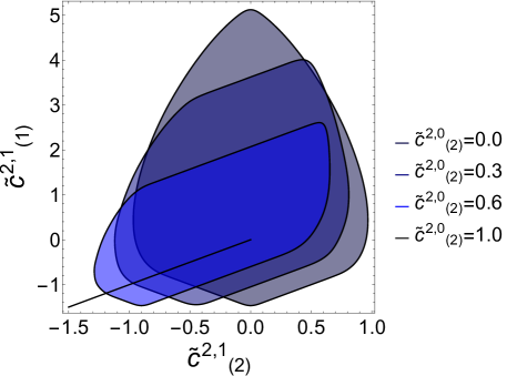
Figure 2: Positivity bounds on $(\tilde{c}_{(2)}^{2,0}=4\tilde{c}^{2,0}_{1122},\tilde{c}_{(1)}^{2,1}=2\tilde{c}_{1111}^{2,1},\tilde{c}_{(2)}^{2,1}=4\tilde{c}^{2,1}_{1122})$ for bi-scalar theory with double $\mathbb{Z}_{2}$ symmetry in the $\tilde{c}^{m,n}_{(3)}=2\tilde{c}^{m,n}_{1221}=0$ subspace, agnostic about all higher order coefficients. $c_{ijkl}^{m,n}$ is the Wilson coefficient in front of the $(s+\frac{t}{2})^{m}t^{n}$ term in the $ij\to kl$ amplitude, and the tilded coefficients are defined as $\tilde{c}_{(a)}^{m,n}\equiv c_{(a)}^{m,n}/c_{(1)}^{2,0}$. We choose units such that the cutoff $\Lambda=1$. We see that the triple crossing positivity bounds form a closed, finite region in the parameter space, numerically of order $\mathcal{O}(1)$.

Higher order coefficients

When moving away from the $c_{(3)}=0$ subspace, the triple crossing bounds are still enclosed, as we shall see now. However, to see that, we need to additionally make use of the upper bounds of the $v^{2}$ coefficients. In this subsection, we shall compute two-sided bounds for the $c_{(a)}^{m\geq 2,n>0}$ coefficients. The two-sided bounds for $c_{(1)}^{m\geq 2,n>0}$ are basically the ones for the single scalar case, for which we can also compute two-sided bounds for $\tilde{c}_{(1)}^{m\geq 2,n>0}$, the ratio between $c_{(1)}^{m\geq 2,n>0}$ and $c_{(1)}^{2,0}$. However, we find that the ratio between $c_{(a\neq 1)}^{m\geq 2,n>0}$ and $c_{(1)}^{2,0}$ is generally unbounded. Nevertheless, as we shall see, $c_{(a\neq 1)}^{m\geq 2,n>0}$ itself is indeed bounded from both sides. This is not surprising as, for the multi-field case, the positivity bounds on the $v^{2}$ coefficients form a multi-dimensional shape and the ratios between themselves are not even fully bounded. Apart from $c_{(2)}^{2h,n}$ and $c_{(3)}^{2h,n}$, we also have another coefficient $c_{(-1)}^{2h+1,n}=4c_{1122}^{2h+1,n}$ for any given $n$ and odd $m=2h+1$, so in this subsection we want to compute the two-sided bounds for the $c_{(2)}^{2h,n}$, $c_{(3)}^{2h,n}$ and $c_{(-1)}^{2h+1,n}$ coefficients.

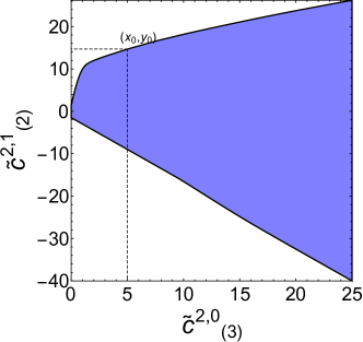
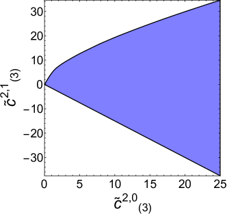
Figure 3: Positivity bounds on $(\tilde{c}_{(3)}^{2,0}=2\tilde{c}_{1212}^{2,0},\tilde{c}_{(2)}^{2,1}=4\tilde{c}^{2,1}_{1122})$ and $(\tilde{c}_{(3)}^{2,0}=2\tilde{c}_{1212}^{2,0},\tilde{c}_{(3)}^{2,1}=2\tilde{c}^{2,1}_{1212})$ for double $\mathbb{Z}_{2}$ symmetric bi-scalar theory. The SDP includes 3 parameters, $c_{(1)}^{2,0}$, $c_{(3)}^{2,0}$ and $c_{(2)}^{2h,n}$, and is agnostic about all other coefficients. In both the left and right plot, the right hand side of the bound extends to infinity.

Let us start with $c_{(2)}^{2,1}$. If we solve SDPs for $\tilde{c}_{(2)}^{2,1}=c_{(2)}^{2,1}/c_{(1)}^{2,0}$, agnostic about all other coefficients, we find it unbounded. (The same applies if we look for bounds on the ratio $c_{(2)}^{2,1}/c_{(2)}^{2,0}$ or $c_{(2)}^{2,1}/c_{(3)}^{2,0}$.) To see this more clearly, let us draw a 2D positivity bound region for $\tilde{c}^{2,1}_{(2)}$ and $\tilde{c}^{2,0}_{(3)}$; see the left plot of Figure 3. (A similar plot can be drawn for $\tilde{c}_{(3)}^{2,1}$ and $\tilde{c}_{(3)}^{2,0}$; see the right plot of Figure 3.) As we can see in this plot, if we look for the triple crossing bounds on $\tilde{c}_{(2)}^{2,1}=c_{(2)}^{2,1}/c_{(1)}^{2,0}$, agnostic about all other coefficients, it is simply unbounded from below and above, which remains true even if we include the upper bound for $c_{(1)}^{2,0}$. This is because, although the $v^{2}$ coefficients are constrained in a finite region, the ratio $\tilde{c}_{(3)}^{2,0}=c_{(3)}^{2,0}/c_{(1)}^{2,0}$ is unbounded from above, which is easy to understand as the positivity region contains points where $c_{(1)}^{2,0}$ approaches to zero but $c_{(3)}^{2,0}$ remains finite. Nevertheless, we can look for the bounds on $c_{(2)}^{2,1}$ itself, and once we also include the generalized upper bounds (90), we can constrain $c_{(2)}^{2,1}$ from both sides. To see how this works, let us look at the example of the upper boundary of the left plot of Figure 3, which starts from near the origin, intersecting with the positive $\tilde{c}^{2,1}_{(2)}$ axis, and extends north-eastward to infinity. Suppose $(x_{0},y_{0})$ is an arbitrary point on this boundary line. For all the points in the positivity region where $\tilde{c}^{2,0}_{(3)}<x_{0}$, we have

$$\tilde{c}^{2,1}_{(2)}=\frac{c^{2,1}_{(2)}}{c^{2,0}_{(1)}}<y_{0}.$$ (96)

Since $0<c^{2,0}_{(1)}<1.588(4\pi)^{2}$, we can infer that $c^{2,1}_{(2)}<y_{0}c^{2,0}_{(1)}<1.588(4\pi)^{2}y_{0}$. For all the points in the positivity region where $\tilde{c}^{2,0}_{(3)}>x_{0}$, on the other hand, we have

$$\frac{c^{2,1}_{(2)}}{c^{2,0}_{(3)}}=\frac{\tilde{c}^{2,1}_{(2)}}{\tilde{c}^{2,0}_{(3)}}<\frac{y_{0}}{x_{0}},$$ (97)

thanks to the fact that the boundaries of positivity bounds are convex. Since $0<c^{2,0}_{(3)}<3.176(4\pi)^{2}$, we can infer that $c^{2,1}_{(2)}<y_{0}c^{2,0}_{(3)}/x_{0}<3.176(4\pi)^{2}y_{0}/x_{0}$. So $c^{2,1}_{(2)}$ must be bounded by the maximum of $1.588(4\pi)^{2}y_{0}$ and $1.588(4\pi)^{2}{2y_{0}}/{x_{0}}$. The optimal upper bound for $c^{2,1}_{(2)}$ is obtained by searching over all $x_{0}$ so as to get the smallest upper bound. Since the upper boundary is convex and monotonically increasing with $x_{0}$, we can infer that $y_{0}$ increases and $2y_{0}/x_{0}$ decreases as $x_{0}$ increases, so the optimal bound is reached at $y_{0}={2y_{0}}/{x_{0}}$, i.e., $\text{min}_{x_{0}}(\text{max}(y_{0},{2y_{0}}/{x_{0}}))=y_{0}|_{x_{0}=2}$. Therefore, we have the optimal upper bound

$$c^{2,1}_{(2)}<1.588(4\pi)^{2}y_{0}|_{x_{0}=2}.$$ (98)

Similarly, we can find a lower bound for $c^{2,1}_{(2)}$ by considering the lower boundary in the left plot of Figure 3, which is given by $c^{2,1}_{(2)}>1.588(4\pi)^{2}y_{0}|_{x_{0}=2}$.

We can apply the above procedure to obtain the two-sided bounds for all the $c_{(2)}^{2h,n}$, $c_{(3)}^{2h,n}$ and $c_{(-1)}^{2h+1,n}$ coefficients, in units of appropriate powers of the cutoff $\Lambda$. Note that for all these coefficients, in the plot similar to those in Figure 3, the upper (lower) boundary must intersect with the positive (negative) axis at $\tilde{c}_{(3)}^{2,0}=0$, as these coefficients being zero must be within the positivity bounds. The two-sided bounds for the first few coefficients in double $\mathbb{Z}_{2}$ bi-scalar theory can be found in Table 1 below:

$$L^{(2)}_{2h,n}<\frac{c_{(2)}^{2h,n}}{(4\pi)^{2}}<U^{(2)}_{2h,n},\leavevmode\nobreak\ \leavevmode\nobreak\ \leavevmode\nobreak\ \leavevmode\nobreak\ \leavevmode\nobreak\ \leavevmode\nobreak\ L^{(3)}_{2h,n}<\frac{c_{(3)}^{2h,n}}{(4\pi)^{2}}<U^{(3)}_{2h,n},\leavevmode\nobreak\ \leavevmode\nobreak\ \leavevmode\nobreak\ \leavevmode\nobreak\ \leavevmode\nobreak\ \leavevmode\nobreak\ L^{(-1)}_{2h+1,n}<\frac{c_{(-1)}^{2h+1,n}}{(4\pi)^{2}}<U^{(-1)}_{2h+1,n},$$ (99)

which are obtained by truncating the null constraints below $p+q=9$ and the partial wave spin below $\ell=50$ but additionally including the $\ell=\infty$ partial wave to speed up the convergence.

$$\begin{array}[]{|c|c|c|c|c|c|c|c|c|c|c|c|}\hline\cr(2h,n)&(2,1)&(2,2)&(4,0)&(2,3)&(4,1)&(2,4)&(4,2)&(6,0)&(2,5)&(4,3)&(6,1)\\ \hline\cr L^{(2)}_{2h,n}&-7.146&-4.320&-4.764&-7.543&-11.910&-1.489&-14.558&-4.764&-7.689&-20.843&-16.674\\ \hline\cr U^{(2)}_{2h,n}&18.981&7.146&4.764&6.536&13.863&17.645&17.865&4.764&2.408&12.367&12.275\\ \hline\cr\hline\cr L^{(3)}_{2h,n}&-4.746&-4.764&0.000&-4.108&-7.940&-5.003&-9.048&0.000&-3.263&-14.871&-11.116\\ \hline\cr U^{(3)}_{2h,n}&12.077&10.787&3.176&10.025&6.539&9.071&13.778&3.176&8.496&11.146&4.948\\ \hline\cr\hline\cr(2h+1,n)&(3,1)&(3,2)&(5,0)&(3,3)&(5,1)&(3,4)&(5,2)&(7,0)&&&\\ \hline\cr\hline\cr L^{(-1)}_{2h+1,n}&-3.176&-12.982&-4.764&-3.972&-7.940&-13.168&-25.990&-4.764&&&\\ \hline\cr U^{(-1)}_{2h+1,n}&16.528&4.140&4.764&12.198&17.463&12.577&8.337&4.764&&&\\ \hline\cr\end{array}$$

Table 1: Two-sided bounds for $c_{(2)}^{2h,n}$, $c_{(3)}^{2h,n}$ and $c_{(-1)}^{2h+1,n}$, for which we are agnostic about all the other coefficients except for the $v^{2}$ coefficients. $L^{(a)}_{m,n}$ and $U^{(a)}_{m,n}$ are defined in Eq. (99). We use the units where the cutoff $\Lambda=1$.

4.2 Bi-scalar theory with $Z_{2}$ symmetry

In the last subsection, we discussed one of the simplest examples of multi-field full crossing bounds and found that the positivity bounds constrain the Wilson coefficients to a small finite region close to the origin. In this subsection, we will slightly increase the complexity by relaxing the symmetries of the theory to consider a bi-scalar theory with $Z_{2}$ symmetry

$$\phi_{i}\rightarrow-\phi_{i},\leavevmode\nobreak\ \leavevmode\nobreak\ i=1,2.$$ (100)

We will see that the Wilson coefficients can still be constrained to a small finite region.

For the $Z_{2}$ bi-scalar theory, $\mathcal{Q}^{ijkl}_{m,n}$ must take the form of Eq. (83), and so its basis can be chosen as

$$\mathcal{Q}_{(1)}=\begin{pmatrix}&1&0&0&0\\ &0&0&0&0\\ &0&0&0&0\\ &0&0&0&0\end{pmatrix},\leavevmode\nobreak\ \leavevmode\nobreak\ \leavevmode\nobreak\ \mathcal{Q}_{(2)}= \begin{pmatrix}&0&0&0&0\\ &0&1&0&0\\ &0&0&0&0\\ &0&0&0&0\end{pmatrix},\leavevmode\nobreak\ \leavevmode\nobreak\ \leavevmode\nobreak\ \mathcal{Q}_{(3)}=\begin{pmatrix}&0&1&0&0\\ &1&0&0&0\\ &0&0&0&1\\ &0&0&1&0\end{pmatrix}$$ (101)

$$\mathcal{Q}_{(4)}=\begin{pmatrix}&0&0&0&0\\ &0&0&0&0\\ &0&0&1&0\\ &0&0&0&1\end{pmatrix} ,\leavevmode\nobreak\ \leavevmode\nobreak\ \leavevmode\nobreak\ \mathcal{Q}_{(-1)}=\begin{pmatrix}&0&1&0&0\\ &1&0&0&0\\ &0&0&0&-1\\ &0&0&-1&0\end{pmatrix}.$$ (102)

With this basis, we have $c_{(1)}^{m,n}=c_{1111}^{m,n},\leavevmode\nobreak\ c_{(2)}^{m,n}=c_{2222}^{m,n},\leavevmode\nobreak\ c_{(3)}^{m,n}=4c_{1122}^{m,n},\leavevmode\nobreak\ c_{(4)}^{m,n}=2c_{1212}^{m,n}$, and other Wilson coefficients are related to the above ones by crossing and internal symmetries. Again, we choose $\mathcal{N}^{ijkl}_{p,q}$ to have the same basis as $\mathcal{Q}^{ijkl}_{2h,n}$. From these bases, we see that the linear matrix inequality can still be cast in a block diagonal form

$$\left(\begin{array}[]{cc}A&0_{2\times 2}\\ 0_{2\times 2}&B\end{array}\right)\succeq 0.$$ (103)

First, we shall explore the shape of the full crossing symmetric bounds on the coefficients of the $v^{2}$ and $v^{2}t$ terms in the $\mathbb{Z}_{2}$ theory. Truncated to this next leading order, we already have 7 parameters: $\tilde{c}_{(2)}^{2,0}$, $\tilde{c}_{(3)}^{2,0}$, $\tilde{c}_{(4)}^{2,0}$, $\tilde{c}_{(1)}^{2,1}$, $\tilde{c}_{(2)}^{2,1}$, $\tilde{c}_{(3)}^{2,1}$ and $\tilde{c}_{(4)}^{2,1}$, if we measure them in terms of $c_{(1)}^{2,0}$. For simplicity, we shall restrict to the subspace $\tilde{c}_{(4)}^{2,0}=\tilde{c}_{(4)}^{2,1}=0$, for which case, the $B\succeq 0$ condition again can be neglected. Then, the SDP problem additionally contains a scaling invariance in the remaining 5D parameter space: $c_{(2)}\rightarrow{\alpha}^{2}c_{(2)},\leavevmode\nobreak\ c_{(3)}\rightarrow{\alpha}c_{(3)}$. To see this, note that the $A$ matrix is explicitly given by

$$A=\begin{pmatrix}&y^{1}_{2,0}\frac{C_{\ell}^{2,0}}{\mu^{3}}+y^{1}_{2,1}\frac{C_{\ell}^{2,1}}{\mu^{4}}+(\text{null-1})&y^{3}_{2,0}\frac{C_{\ell}^{2,0}}{\mu^{3}}+y^{3}_{2,1}\frac{C_{\ell}^{2,1}}{\mu^{4}}+(\text{null-2})\\ &y^{3}_{2,0}\frac{C_{\ell}^{2,0}}{\mu^{3}}+y^{3}_{2,1}\frac{C_{\ell}^{2,1}}{\mu^{4}}+(\text{null-2})&y^{2}_{2,0}\frac{C_{\ell}^{2,0}}{\mu^{3}}+y^{2}_{2,1}\frac{C_{\ell}^{2,1}}{\mu^{4}}+(\text{null-3})\end{pmatrix},$$ (104)

where $(\text{null-1})$ to $(\text{null-4})$ are four different sums of the null constraints. $A$ being semi-definite positive is equivalent to $A_{11}\geq 0$, $A_{22}\geq 0$ and $A_{11}A_{22}\geq(A_{12})^{2}$, and the objective is to minimize $y^{1}_{2,0}c_{(1)}^{2,0}+y^{2}_{2,0}c_{(2)}^{2,0}+y^{3}_{2,0}c_{(3)}^{2,0}+y^{2}_{2,1}c_{(2)}^{2,1}+y^{3}_{2,1}c_{(3)}^{2,1}$. Clearly, we can re-write the objective and the constraints as

minimize $$y^{1}_{2,0}+\bar{y}^{2}_{2,0}\left({\alpha}^{2}c_{(2)}^{2,0}\right)+\bar{y}^{3}_{2,0}\left({\alpha}c_{(3)}^{2,0}\right)+\bar{y}^{2}_{2,1}\left({\alpha}^{2}c_{(2)}^{2,1}\right)+\bar{y}^{3}_{2,1}\left({\alpha}c_{(3)}^{2,1}\right)$$ (105)

subject to $$A_{11}\geq 0,\leavevmode\nobreak\ \leavevmode\nobreak\ \left(A_{22}|_{y^{2}\to\bar{y}^{2},z^{2}\to\bar{z}^{2}}\right)\geq 0,\leavevmode\nobreak\ \leavevmode\nobreak\ A_{11}\left(A_{22}|_{y^{2}\to\bar{y}^{2},z^{2}\to\bar{z}^{2}}\right)\geq\left(A_{12}|_{y^{3}\to\bar{y}^{3},z^{3}\to\bar{z}^{3}}\right)^{2},$$ (106)

where we have defined $\bar{y}^{2}\equiv y^{2}/{\alpha}^{2},\leavevmode\nobreak\ \bar{y}^{3}\equiv y^{3}/{\alpha}$, and $|_{y^{2}\to\bar{y}^{2}}$, for example, means replacing $y^{2}_{2,0}$ and $y^{2}_{2,1}$ in $A_{22}$ with $\bar{y}^{2}_{2,0}$ and $\bar{y}^{2}_{2,1}$ respectively. The scaled SDP is the same as the original SDP but with scaled coefficients ${\alpha}^{2}c_{(2)}$ and ${\alpha}c_{(3)}$. We can use this scaling invariance to set $\tilde{c}_{(2)}^{2,0}=1$ without loss of generality, and we are left 4 Wilson coefficients $\tilde{c}_{(3)}^{2,0}$, $\tilde{c}_{(1)}^{2,1}$, $\tilde{c}_{(2)}^{2,1}$, $\tilde{c}_{(3)}^{2,1}$.

Of course, we still can not visualize 4D parameter space, so we will plot the positivity bounds for different $\tilde{c}_{(3)}^{2,0}$. From the results of the $v^{2}$ convex cone, we know that viable $\tilde{c}_{(3)}^{2,0}$ must be in the range Li:2021lpe : $-2\leq\tilde{c}_{(3)}^{2,0}\leq 2$, which is symmetric with respect to $\tilde{c}_{(3)}^{2,0}=0$. To probe how the positivity region varies with different $\tilde{c}_{(3)}^{2,0}$, we shall look at 3 slices of the 4D parameter space, and we will see that on all of them the 3D parameter space $(\tilde{c}_{(1)}^{2,1},\leavevmode\nobreak\ \tilde{c}_{(2)}^{2,1},\leavevmode\nobreak\ \tilde{c}_{(3)}^{2,1})$ is constrained to a finite region.

• The $\tilde{c}_{(3)}^{2,0}=2.0$ slice: Since it is at one of the extremities of $\tilde{c}_{(3)}^{2,0}$, the allowed region is a line segment

  $$\tilde{c}^{2,1}_{(1)}=\tilde{c}^{2,1}_{(2)}=\frac{1}{2}\tilde{c}^{2,1}_{(3)}=\eta,\leavevmode\nobreak\ \leavevmode\nobreak\ -1.5\leq\eta\leq 0.$$ (107)

  

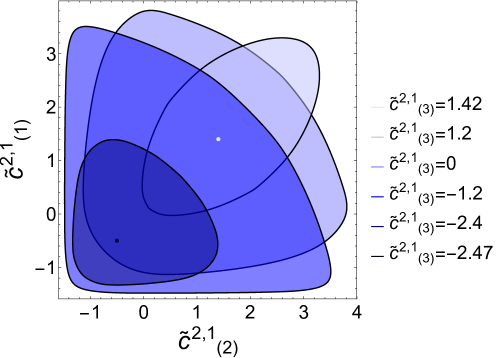
  Figure 4: Positivity bounds on $(\tilde{c}_{(1)}^{2,1}=\tilde{c}^{2,1}_{1111},\tilde{c}_{(2)}^{2,1}=\tilde{c}^{2,1}_{2222},\tilde{c}_{(3)}^{2,1}=4\tilde{c}^{2,1}_{1122})$ for $\mathbb{Z}_{2}$ symmetric bi-scalar theory on the $\tilde{c}_{(3)}^{2,0}=1.0$ slice. The tildes on the coefficients mean that they are divided by $c_{(1)}^{2,0}$. We have truncated up to order $(m=2,n=1)$, restricted to $\tilde{c}_{(4)}^{2,0}=\tilde{c}_{(4)}^{2,1}=0$ and set $\tilde{c}_{(2)}^{2,0}$ to 1 (without loss of generality). We choose units such that the cutoff $\Lambda=1$.

• The $\tilde{c}_{(3)}^{2,0}=1.0$ slice: We now need to numerically running the SDP for many sets of Wilson coefficients to get contour plots for different values of $\tilde{c}_{(3)}^{2,1}$. Notice that the plots are symmetric in exchanging $\tilde{c}_{(1)}^{2,1}\leftrightarrow\tilde{c}_{(2)}^{2,1}$, which is not surprising since we have chosen $\tilde{c}_{(2)}^{2,0}=1=\tilde{c}_{(1)}^{2,0}$. As shown in Figure 4, $\tilde{c}_{(3)}^{2,1}$ has an upper bound $\tilde{c}_{(3)}^{2,1}=1.42$ and a lower bound $\tilde{c}_{(3)}^{2,1}=-2.47$.

  

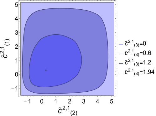
  Figure 5: Positivity bounds on $(\tilde{c}_{(1)}^{2,1}=\tilde{c}^{2,1}_{1111},\tilde{c}_{(2)}^{2,1}=\tilde{c}^{2,1}_{2222},\tilde{c}_{(3)}^{2,1}=4\tilde{c}^{2,1}_{1122})$ for $\mathbb{Z}_{2}$ symmetric bi-scalar theory on the $\tilde{c}_{(3)}^{2,0}=0.0$ slice.

• The $\tilde{c}_{(3)}^{2,0}=0.0$ slice: We find that $\tilde{c}_{(1)}^{2,1}$ and $\tilde{c}_{(2)}^{2,1}$ reach both their lower limit ($-1.5$) and upper limit ($5.173$) when $\tilde{c}_{(3)}^{2,1}=0$, which are the box bounds in Figure 5, the 2D generalization of the two-sided bounds for single scalar scattering. On the other hand, $\tilde{c}_{(3)}^{2,1}$ reaches both of its lower and upper limit at $\tilde{c}_{(3)}^{2,1}=\pm 1.94$.

We can also consider two-sided bounds for the $\mathbb{Z}_{2}$ theory, i.e., the bounds on $c^{2h,n}_{(3)}$, $c^{2h,n}_{(4)}$ and $c^{2h+1,n}_{(-1)}$. The two-sided bounds on $c^{2h,n}_{(1)}$ and $c^{2h,n}_{(2)}$ are the bounds in the single scalar case. Since the positivity region is convex, the positivity bounds must be symmetric in exchanging $c_{(1)}^{m,n}\leftrightarrow c_{(2)}^{m,n}$, and so the weakest bounds must occur in the subspace $c_{(1)}^{m,n}=c_{(2)}^{m,n}$. If we have $c_{(1)}^{m,n}=c_{(2)}^{m,n}$, we effectively reduce back to the double $\mathbb{Z}_{2}$ case. So the two-sided bounds on $c^{2h,n}_{(3)}$, $c^{2h,n}_{(4)}$ and $c^{2h+1,n}_{(-1)}$ here are exactly the same as those on $c^{2h,n}_{(2)}$, $c^{2h,n}_{(3)}$ and $c^{2h+1,n}_{(-1)}$ in the double $\mathbb{Z}_{2}$ theory. Notice that in our notation $c^{2h,n}_{(3)}$ and $c^{2h,n}_{(4)}$ here are the same as the $c^{2h,n}_{(2)}$ and $c^{2h,n}_{(3)}$ in the double $\mathbb{Z}_{2}$ theory.

Appendix A Expressions for $\bar{n}^{p,q}_{ijkl}$, $E^{\pm}_{p,q}$ and $F^{\pm}_{p,q}$

While the $jl$ symmetrized null constraints $n^{p,q}_{ijkl}=0$ are sufficient for our approach with the $su$ symmetric dispersive relation, it is conceivable that the unprojected null constraints $\bar{n}^{p,q}_{ijkl}=0$ can be useful in other approaches. Here we also list the first few $\bar{n}^{p,q}_{ijkl}$ null constraints for a comparison:

$$\bar{n}_{ijkl}^{1,3} =\bar{n}_{ijkl}^{2,2}=c_{ijkl}^{2,2}+\frac{3}{2}(c_{ijkl}^{3,1}+c_{ijkl}^{4,0})-c_{ikjl}^{2,2}-\frac{3}{2}(c_{ikjl}^{3,1}+c_{ikjl}^{4,0})=0$$ (108)

$$\bar{n}_{ijkl}^{1,4} =c_{ijkl}^{2,3}+\frac{3}{4}c_{ijkl}^{3,2}-\frac{5}{8}c_{ijkl}^{5,0}+\frac{3}{4}c_{ikjl}^{2,3}+\frac{1}{8}c_{ikjl}^{3,2}-\frac{7}{8}c_{ikjl}^{4,1}-\frac{25}{16}c_{ikjl}^{5,0}=0$$ (109)

$$\bar{n}_{ijkl}^{2,3} =c_{ijkl}^{2,3}+\frac{3}{2}c_{ijkl}^{3,2}+\frac{3}{2}c_{ijkl}^{4,1}+\frac{5}{4}c_{ijkl}^{5,0}-c_{ikjl}^{3,2}-2c_{ikjl}^{4,1}-\frac{5}{2}c_{ikjl}^{5,0}=0$$ (110)

$$\bar{n}_{ijkl}^{1,5} =c_{ijkl}^{2,2}+\frac{3}{4}c_{ijkl}^{3,3}+\frac{1}{2}c_{ijkl}^{4,2}+\frac{5}{8}c_{ijkl}^{5,1}+\frac{15}{16}c_{ijkl}^{6,0}-\frac{1}{2}c_{ikjl}^{2,4}-\frac{1}{4}c_{ikjl}^{4,2}-\frac{5}{4}c_{ikjl}^{5,1}-\frac{75}{32}c_{ikjl}^{6,0}=0$$ (111)

$$\bar{n}_{ijkl}^{2,4} =c_{ijkl}^{2,4}+\frac{3}{2}c_{ijkl}^{3,3}+\frac{3}{2}c_{ijkl}^{4,2}+\frac{5}{4}c_{ijkl}^{5,1}+\frac{15}{16}c_{ijkl}^{6,0}-c_{ikjl}^{4,2}-\frac{5}{2}c_{ikjl}^{5,1}-\frac{15}{4}c_{ikjl}^{6,0}=0$$ (112)

$$\bar{n}_{ijkl}^{3,3} =c_{ijkl}^{3,3}+2c_{ijkl}^{4,2}+\frac{5}{2}(c_{ijkl}^{5,1}+c_{ijkl}^{6,0})-c_{ikjl}^{3,3}-2c_{ikjl}^{4,2}-\frac{5}{2}(c_{ikjl}^{5,1}+c_{ikjl}^{6,0})=0.$$ (113)

They are mostly the same as $n^{p,q}_{ijkl}=0$ except for $(p,q)=(1,3),(1,4),(1,5),...\,$. The corresponding explicit expressions of $E^{\pm}_{p,q}$ and $F^{\pm}_{p,q}$ for the first few $\bar{n}^{p,q}_{ijkl}$ null constraints in 4D (remove the parts in the square brackets to get $E^{\pm}_{p,q}$ and $F^{\pm}_{p,q}$ for the $n^{p,q}_{ijkl}$ null constraints) are given by

$$E^{+}_{1,3} =\frac{1}{2}(\ell^{4}+2\ell^{3}-7\ell^{2}-8\ell+8)+\bigg{[}2\bigg{]}$$ (114)

$$F^{+}_{1,3} =-4+\bigg{[}\frac{1}{2}(-\ell^{4}-2\ell^{3}+7\ell^{2}+8\ell-6)+1\bigg{]}$$ (115)

$$E^{-}_{1,3} =\frac{3}{2}(\ell^{2}+\ell-2)+\bigg{[}\frac{3}{2}(\ell^{2}+\ell-2)\bigg{]}$$ (116)

$$F^{-}_{1,3} =-2(\ell^{2}+\ell-2)+\bigg{[}-\ell^{2}-\ell+2\bigg{]}$$ (117)

$$E^{+}_{2,2} =\frac{\ell^{4}}{2}+\ell^{3}-\frac{7\ell^{2}}{2}-4\ell+6$$ (118)

$$F^{+}_{2,2} =-\frac{\ell^{4}}{2}-\ell^{3}+\frac{7\ell^{2}}{2}+4\ell-6$$ (119)

$$E^{-}_{2,2} =3(\ell^{2}+\ell-2)$$ (120)

$$F^{-}_{2,2} =-3(\ell^{2}+\ell-2)$$ (121)

$$E^{+}_{1,4} =\frac{1}{36}(2\ell^{6}+6\ell^{5}-37\ell^{4}-84\ell^{3}+179\ell^{2}+222\ell-180)+\bigg{[}\frac{1}{2}(-2\ell^{2}-2\ell+5)\bigg{]}$$ (122)

$$F^{+}_{1,4} =-2\ell^{2}-2\ell+5+\bigg{[}\frac{1}{48}(2\ell^{6}+6\ell^{5}-37\ell^{4}-84\ell^{3}+155\ell^{2}+198\ell-120)\bigg{]}$$ (123)

$$E^{-}_{1,4} =\frac{1}{8}(3\ell^{4}+6\ell^{3}-27\ell^{2}-30\ell+35)+\bigg{[}\frac{15}{8}\bigg{]}$$ (124)

$$F^{-}_{1,4} =-5+\bigg{[}\frac{1}{16}(\ell^{4}+2\ell^{3}-9\ell^{2}-10\ell+40)\bigg{]}$$ (125)

$$E^{+}_{2,3} =\frac{1}{36}(2\ell^{6}+6\ell^{5}-37\ell^{4}-84\ell^{3}+251\ell^{2}+294\ell-360)$$ (126)

$$F^{+}_{2,3} =-4\ell^{2}-4\ell+10$$ (127)

$$E^{-}_{2,3} =\frac{1}{4}(3\ell^{4}+6\ell^{3}-27\ell^{2}-30\ell+40)$$ (128)

$$F^{-}_{2,3} =-\frac{1}{2}\ell^{4}-\ell^{3}+\frac{9}{2}\ell^{2}+5\ell-10$$ (129)

$$E^{+}_{1,5} =\frac{1}{288}(\ell^{8}+4\ell^{7}-38\ell^{6}-128\ell^{5}+457\ell^{4}+1132\ell^{3}-1860\ell^{2}-2448\ell+1728)+\bigg{[}\frac{3}{2}\bigg{]}$$ (130)

$$F^{+}_{1,5} =-6+\bigg{[}\frac{1}{576}(-\ell^{8}-4\ell^{7}+38\ell^{6}+128\ell^{5}-457\ell^{4}-1132\ell^{3}+1860\ell^{2}+2448\ell-864)\bigg{]}$$ (131)

$$E^{-}_{1,5} =\frac{1}{24}(\ell^{6}+3\ell^{5}-23\ell^{4}-51\ell^{3}+127\ell^{2}+153\ell-135)+\bigg{[}\frac{5}{8}(\ell^{2}+\ell-3)\bigg{]}$$ (132)

$$F^{-}_{1,5} =-2(\ell^{2}+\ell-3)+\bigg{[}\frac{1}{2}(-\ell^{2}-\ell+3)\bigg{]}$$ (133)

$$E^{+}_{2,4} =\frac{1}{288}(\ell^{8}+4\ell^{7}-38\ell^{6}-128\ell^{5}+601\ell^{4}+1420\ell^{3}-3444\ell^{2}-4176\ell+4320)$$ (134)

$$F^{+}_{2,4} =-\frac{\ell^{4}}{2}-\ell^{3}+\frac{11\ell^{2}}{2}+6\ell-15$$ (135)

$$E^{-}_{2,4} =\frac{1}{12}(\ell^{6}+3\ell^{5}-23\ell^{4}-51\ell^{3}+142\ell^{2}+168\ell-180)$$ (136)

$$F^{-}_{2,4} =-5(\ell^{2}+\ell-3)$$ (137)

$$E^{+}_{3,3} =\ell^{4}+2\ell^{3}-11\ell^{2}-12\ell+20$$ (138)

$$F^{+}_{3,3} =-\ell^{4}-2\ell^{3}+11\ell^{2}+12\ell-20$$ (139)

$$E^{-}_{3,3} =\frac{1}{18}(\ell^{6}+3\ell^{5}-23\ell^{4}-51\ell^{3}+202\ell^{2}+228\ell-360)$$ (140)

$$F^{-}_{3,3} =\frac{1}{18}(-\ell^{6}-3\ell^{5}+23\ell^{4}+51\ell^{3}-202\ell^{2}-228\ell+360).$$ (141)

Note that we have artificially separated the 13, 14, 15 components of the $E$ and $F$ quantities into to two parts. The parts outside the square bracket is the $E$ and $F$ quantities corresponding to the $n^{p,q}_{ijkl}$ null constraints, that is, the parts in the square bracket is projected out if we symmetrize the $jl$ indices for $\bar{n}^{p,q}_{ijkl}=0$. Without the square bracket parts, the null constraints directly reduce to the null constraints for the case of identical scalar scattering in Tolley:2020gtv ; otherwise they may reduce to some superpositions of these null constraints.

Appendix B The case for massive fields

In the main text, we assumed that the hierarchy between the masses of the IR and UV particles is so large that we can treat the IR particles as effectively massless. However, this may not aways be the case. Take one of the earliest EFT, SU(2) chiral perturbation theory for strong interactions, for example. The ratio between the pion threshold and the cutoff is only about 0.24, in which case the masses of the IR modes can introduce significant corrections to the positivity bounds Manohar:2008tc ; Wang:2020jxr . In general, if the particles are of different masses, forming the positivity bounds as a polynomial matrix program with only continuous variable appears to be elusive. This is because, for the general case, $s+t+u=m_{i}^{2}+m_{j}^{2}+m_{k}^{2}+m_{l}^{2}$ will appear in the denominator of the crossed $u$ channel, and the kinematics will now be very complicated, which leads to a very awkward expression for $\cos\theta$ in the partial wave expansion, so that the partial wave expansion depends on the particle masses $m_{i},m_{j},m_{k},m_{l}$ highly nonlinearly. Nevertheless, if all the modes are of the same mass $m$ such as those in a symmetry multiplet, it is straightforward to generalize our formalism to include the mass corrections.

We can essentially follow the same steps as the massless case. The differences are that now we define the $v$ variable and the subtraction point $\mu_{p}$ as

$$v=s+\frac{t}{2}-2m^{2},\leavevmode\nobreak\ \leavevmode\nobreak\ \leavevmode\nobreak\ \leavevmode\nobreak\ \leavevmode\nobreak\ \mu_{p}=2m^{2}-\frac{t}{2},$$ (142)

which leads to the following dispersion relation for the pole-removed amplitude

$$B_{ijkl}(s,t) =A_{ijkl}(s,t)-\frac{{\lambda}_{ijkl}}{m^{2}-s}-\frac{{\lambda}_{ijkl}}{m^{2}-t}-\frac{{\lambda}_{ijkl}}{m^{2}-u}$$ (143)

$$=\tilde{a}^{(0)}_{ijkl}(t)+a^{(1)}_{ijkl}(t)v+v^{2}\int^{\infty}_{4m^{2}}\frac{\mathrm{d}\mu}{\pi(\mu-2m^{2}+\frac{t}{2})^{2}}\left[\frac{{\rm Abs}\,A_{ijkl}(\mu,t)}{\mu-2m^{2}+\frac{t}{2}-v}+\frac{{\rm Abs}\,A_{ilkj}(\mu,t)}{\mu-2m^{2}+\frac{t}{2}+v}\right]$$

$$=\tilde{a}^{(0)}_{ijkl}(t)+a^{(1)}_{ijkl}(t)v+v^{2}\int^{\infty}_{2m^{2}}\frac{\mathrm{d}\mu}{\pi(\mu+\frac{t}{2})^{2}}\left[\frac{{\rm Abs}\,A_{ijkl}(\mu+2m^{2},t)}{\mu+\frac{t}{2}-v}+\frac{{\rm Abs}\,A_{ilkj}(\mu+2m^{2},t)}{\mu+\frac{t}{2}+v}\right],$$

where in the last step we have shifted the integration variable by $2m^{2}$. Note that if desirable we could also subtract out the known low energy contribution of the dispersive integral from $4m^{2}$ to $\Lambda^{2}$ as we did in the main text. The absorptive part of the amplitude in the massive case can be expanded by partial waves as follows

$${\rm Abs}\,A_{ijkl}(\mu,t)=\frac{2^{4{\alpha}+2}\pi^{\alpha}\Gamma({\alpha})\mu^{\frac{1}{2}}}{{(\mu-4m^{2})}^{{\alpha}}}\sum_{\ell=0}^{\infty}(2\ell+2{\alpha})C^{({\alpha})}_{\ell}\left(1+\frac{2t}{\mu-4m^{2}}\right){\rm Abs}\,a^{ijkl}_{\ell}(\mu),\leavevmode\nobreak\ \leavevmode\nobreak\ \leavevmode\nobreak\ {\alpha}=\frac{D-3}{2},$$ (144)

Expanding both sides of the dispersion relation, we can get the sum rules for the massive case:

$$c_{ijkl}^{m,n}=\left\langle C_{ijkl}^{m,n}\right\rangle\equiv\left\langle\left[m_{\ell}^{ij}(m_{\ell}^{kl})^{*}+(-1)^{m}m_{\ell}^{il}(m_{\ell}^{kj})^{*}\right]\tilde{C}_{\ell}^{m,n}(\mu)\right\rangle,\leavevmode\nobreak\ \leavevmode\nobreak\ m\geq 2,n\geq 0,$$ (145)

where $\tilde{C}_{\ell}^{m,n}$ is now given by

$$\tilde{C}_{\ell}^{m,n}(\mu)=\sum_{p=0}^{n}\frac{L^{p}_{\ell}H^{n-p}_{m+1}}{\mu^{m+1+p}(\mu-2m^{2})^{n-p}}.$$ (146)

With these established, we can follow the same steps as the massless case to obtain the positivity bounds with SDPB.

References

- (1) A. Adams, N. Arkani-Hamed, S. Dubovsky, A. Nicolis and R. Rattazzi, Causality, analyticity and an IR obstruction to UV completion, JHEP 10 (2006) 014, [hep-th/0602178].
- (2) T. N. Pham and T. N. Truong, Evaluation of the Derivative Quartic Terms of the Meson Chiral Lagrangian From Forward Dispersion Relation, Phys. Rev. D31 (1985) 3027.
- (3) B. Ananthanarayan, D. Toublan and G. Wanders, Consistency of the chiral pion pion scattering amplitudes with axiomatic constraints, Phys. Rev. D51 (1995) 1093–1100, [hep-ph/9410302].
- (4) N. Arkani-Hamed, T.-C. Huang and Y.-T. Huang, The EFT-Hedron, JHEP 05 (2021) 259, [2012.15849].
- (5) B. Bellazzini, J. Elias Miró, R. Rattazzi, M. Riembau and F. Riva, Positive moments for scattering amplitudes, Phys. Rev. D 104 (2021) 036006, [2011.00037].
- (6) C. de Rham, S. Melville, A. J. Tolley and S.-Y. Zhou, Positivity bounds for scalar field theories, Phys. Rev. D96 (2017) 081702, [1702.06134].
- (7) A. V. Manohar and V. Mateu, Dispersion Relation Bounds for pi pi Scattering, Phys. Rev. D77 (2008) 094019, [0801.3222].
- (8) A. Nicolis, R. Rattazzi and E. Trincherini, Energy’s and amplitudes’ positivity, JHEP 05 (2010) 095, [0912.4258].
- (9) B. Bellazzini, Softness and amplitudes’ positivity for spinning particles, JHEP 02 (2017) 034, [1605.06111].
- (10) C. de Rham, S. Melville, A. J. Tolley and S.-Y. Zhou, UV complete me: Positivity Bounds for Particles with Spin, JHEP 03 (2018) 011, [1706.02712].
- (11) A. J. Tolley, Z.-Y. Wang and S.-Y. Zhou, New positivity bounds from full crossing symmetry, JHEP 05 (2021) 255, [2011.02400].
- (12) S. Caron-Huot and V. Van Duong, Extremal Effective Field Theories, JHEP 05 (2021) 280, [2011.02957].
- (13) D. Simmons-Duffin, A Semidefinite Program Solver for the Conformal Bootstrap, JHEP 06 (2015) 174, [1502.02033].
- (14) A. Sinha and A. Zahed, Crossing Symmetric Dispersion Relations in Quantum Field Theories, Phys. Rev. Lett. 126 (2021) 181601, [2012.04877].
- (15) G. Auberson and N. N. Khuri, Rigorous parametric dispersion representation with three-channel symmetry, Phys. Rev. D 6 (1972) 2953–2966.
- (16) L.-Y. Chiang, Y.-t. Huang, W. Li, L. Rodina and H.-C. Weng, Into the EFThedron and UV constraints from IR consistency, 2105.02862.
- (17) A. Nicolis, R. Rattazzi and E. Trincherini, The Galileon as a local modification of gravity, Phys. Rev. D 79 (2009) 064036, [0811.2197].
- (18) C. de Rham, J. T. Deskins, A. J. Tolley and S.-Y. Zhou, Graviton Mass Bounds, Rev. Mod. Phys. 89 (2017) 025004, [1606.08462].
- (19) S. Caron-Huot, D. Mazac, L. Rastelli and D. Simmons-Duffin, Sharp Boundaries for the Swampland, JHEP 07 (2021) 110, [2102.08951].
- (20) B. Bellazzini, C. Cheung and G. N. Remmen, Quantum Gravity Constraints from Unitarity and Analyticity, Phys. Rev. D93 (2016) 064076, [1509.00851].
- (21) C. Cheung and G. N. Remmen, Positive Signs in Massive Gravity, JHEP 04 (2016) 002, [1601.04068].
- (22) J. Bonifacio, K. Hinterbichler and R. A. Rosen, Positivity constraints for pseudolinear massive spin-2 and vector Galileons, Phys. Rev. D94 (2016) 104001, [1607.06084].
- (23) C. de Rham, S. Melville, A. J. Tolley and S.-Y. Zhou, Massive Galileon Positivity Bounds, JHEP 09 (2017) 072, [1702.08577].
- (24) B. Bellazzini, F. Riva, J. Serra and F. Sgarlata, Beyond Positivity Bounds and the Fate of Massive Gravity, Phys. Rev. Lett. 120 (2018) 161101, [1710.02539].
- (25) C. de Rham, S. Melville, A. J. Tolley and S.-Y. Zhou, Positivity Bounds for Massive Spin-1 and Spin-2 Fields, 1804.10624.
- (26) J. Bonifacio and K. Hinterbichler, Bounds on Amplitudes in Effective Theories with Massive Spinning Particles, 1804.08686.
- (27) S. Melville and J. Noller, Positivity in the Sky: Constraining dark energy and modified gravity from the UV, Phys. Rev. D 101 (2020) 021502, [1904.05874].
- (28) C. de Rham and A. J. Tolley, Speed of gravity, Phys. Rev. D 101 (2020) 063518, [1909.00881].
- (29) L. Alberte, C. de Rham, A. Momeni, J. Rumbutis and A. J. Tolley, Positivity Constraints on Interacting Spin-2 Fields, JHEP 03 (2020) 097, [1910.11799].
- (30) L. Alberte, C. de Rham, S. Jaitly and A. J. Tolley, QED positivity bounds, Phys. Rev. D 103 (2021) 125020, [2012.05798].
- (31) W.-M. Chen, Y.-T. Huang, T. Noumi and C. Wen, Unitarity bounds on charged/neutral state mass ratios, Phys. Rev. D 100 (2019) 025016, [1901.11480].
- (32) Y.-t. Huang, J.-Y. Liu, L. Rodina and Y. Wang, Carving out the Space of Open-String S-matrix, JHEP 04 (2021) 195, [2008.02293].
- (33) L. Alberte, C. de Rham, S. Jaitly and A. J. Tolley, Positivity Bounds and the Massless Spin-2 Pole, 2007.12667.
- (34) J. Tokuda, K. Aoki and S. Hirano, Gravitational positivity bounds, JHEP 11 (2020) 054, [2007.15009].
- (35) Z.-Y. Wang, C. Zhang and S.-Y. Zhou, Generalized elastic positivity bounds on interacting massive spin-2 theories, JHEP 04 (2021) 217, [2011.05190].
- (36) M. Herrero-Valea, I. Timiryasov and A. Tokareva, To Positivity and Beyond, where Higgs-Dilaton Inflation has never gone before, JCAP 11 (2019) 042, [1905.08816].
- (37) M. Herrero-Valea, R. Santos-Garcia and A. Tokareva, Massless positivity in graviton exchange, Phys. Rev. D 104 (2021) 085022, [2011.11652].
- (38) C. de Rham, S. Melville and J. Noller, Positivity bounds on dark energy: when matter matters, JCAP 08 (2021) 018, [2103.06855].
- (39) D. Traykova, E. Bellini, P. G. Ferreira, C. Garcia-Garcia, J. Noller and M. Zumalacarregui, Theoretical priors in scalar-tensor cosmologies: Shift-symmetric Horndeski models, Phys. Rev. D 104 (2021) 083502, [2103.11195].
- (40) Z. Bern, D. Kosmopoulos and A. Zhiboedov, Gravitational effective field theory islands, low-spin dominance, and the four-graviton amplitude, J. Phys. A 54 (2021) 344002, [2103.12728].
- (41) N. Arkani-Hamed, Y.-t. Huang, J.-Y. Liu and G. N. Remmen, Causality, Unitarity, and the Weak Gravity Conjecture, 2109.13937.
- (42) A.-C. Davis and S. Melville, Scalar Fields Near Compact Objects: Resummation versus UV Completion, 2107.00010.
- (43) C. Zhang and S.-Y. Zhou, Convex Geometry Perspective on the (Standard Model) Effective Field Theory Space, Phys. Rev. Lett. 125 (2020) 201601, [2005.03047].
- (44) X. Li, H. Xu, C. Yang, C. Zhang and S.-Y. Zhou, Positivity in Multifield Effective Field Theories, Phys. Rev. Lett. 127 (2021) 121601, [2101.01191].
- (45) C. Zhang and S.-Y. Zhou, Positivity bounds on vector boson scattering at the LHC, Phys. Rev. D100 (2019) 095003, [1808.00010].
- (46) Q. Bi, C. Zhang and S.-Y. Zhou, Positivity constraints on aQGC: carving out the physical parameter space, JHEP 06 (2019) 137, [1902.08977].
- (47) K. Yamashita, C. Zhang and S.-Y. Zhou, Elastic positivity vs extremal positivity bounds in SMEFT: a case study in transversal electroweak gauge-boson scatterings, JHEP 01 (2021) 095, [2009.04490].
- (48) B. Fuks, Y. Liu, C. Zhang and S.-Y. Zhou, Positivity in electron-positron scattering: testing the axiomatic quantum field theory principles and probing the existence of UV states, Chin. Phys. C 45 (2021) 023108, [2009.02212].
- (49) J. Gu, L.-T. Wang and C. Zhang, An unambiguous test of positivity at lepton colliders, 2011.03055.
- (50) L. Vecchi, Causal versus analytic constraints on anomalous quartic gauge couplings, JHEP 11 (2007) 054, [0704.1900].
- (51) B. Bellazzini and F. Riva, New phenomenological and theoretical perspective on anomalous ZZ and Z processes, Phys. Rev. D 98 (2018) 095021, [1806.09640].
- (52) G. N. Remmen and N. L. Rodd, Consistency of the Standard Model Effective Field Theory, JHEP 12 (2019) 032, [1908.09845].
- (53) T. Trott, Causality, Unitarity and Symmetry in Effective Field Theory, 2011.10058.
- (54) G. N. Remmen and N. L. Rodd, Flavor Constraints from Unitarity and Analyticity, Phys. Rev. Lett. 125 (2020) 081601, [2004.02885].
- (55) Q. Bonnefoy, E. Gendy and C. Grojean, Positivity bounds on Minimal Flavor Violation, JHEP 04 (2021) 115, [2011.12855].
- (56) M. Chala and J. Santiago, Positivity bounds in the Standard Model effective field theory beyond tree level, 2110.01624.
- (57) J. Distler, B. Grinstein, R. A. Porto and I. Z. Rothstein, Falsifying Models of New Physics via WW Scattering, Phys. Rev. Lett. 98 (2007) 041601, [hep-ph/0604255].
- (58) G. N. Remmen and N. L. Rodd, Signs, Spin, SMEFT: Positivity at Dimension Six, 2010.04723.
- (59) T. Grall and S. Melville, Positivity Bounds without Boosts, 2102.05683.
- (60) J. Davighi, S. Melville and T. You, Natural Selection Rules: New Positivity Bounds for Massive Spinning Particles, 2108.06334.
- (61) P. Haldar, A. Sinha and A. Zahed, Quantum field theory and the Bieberbach conjecture, SciPost Phys. 11 (2021) 002, [2103.12108].
- (62) P. Raman and A. Sinha, QFT, EFT and GFT, 2107.06559.
- (63) R. Gopakumar, A. Sinha and A. Zahed, Crossing Symmetric Dispersion Relations for Mellin Amplitudes, Phys. Rev. Lett. 126 (2021) 211602, [2101.09017].
- (64) A. Zahed, Positivity and Geometric Function Theory Constraints on Pion Scattering, 2108.10355.
- (65) S. Kundu, Swampland Conditions for Higher Derivative Couplings from CFT, 2104.11238.
- (66) M. F. Paulos, J. Penedones, J. Toledo, B. C. van Rees and P. Vieira, The S-matrix bootstrap. Part I: QFT in AdS, JHEP 11 (2017) 133, [1607.06109].
- (67) A. L. Guerrieri, J. Penedones and P. Vieira, S-matrix bootstrap for effective field theories: massless pions, JHEP 06 (2021) 088, [2011.02802].
- (68) A. Hebbar, D. Karateev and J. Penedones, Spinning S-matrix Bootstrap in 4d, 2011.11708.
- (69) A. Guerrieri and A. Sever, Rigorous bounds on the Analytic -matrix, 2106.10257.
- (70) M. Froissart, Asymptotic behavior and subtractions in the Mandelstam representation, Phys. Rev. 123 (1961) 1053–1057.
- (71) A. Martin, Unitarity and high-energy behavior of scattering amplitudes, Phys. Rev. 129 (1963) 1432–1436.
- (72) D. Poland, S. Rychkov and A. Vichi, The Conformal Bootstrap: Theory, Numerical Techniques, and Applications, Rev. Mod. Phys. 91 (2019) 015002, [1805.04405].
- (73) Y.-J. Wang, F.-K. Guo, C. Zhang and S.-Y. Zhou, Generalized positivity bounds on chiral perturbation theory, JHEP 07 (2020) 214, [2004.03992].