The SPDE approach for Gaussian and non-Gaussian fields:
10
years and still running
Abstract
Gaussian processes and random fields have a long history, covering multiple approaches to representing spatial and spatio-temporal dependence structures, such as covariance functions, spectral representations, reproducing kernel Hilbert spaces, and graph based models. This article describes how the stochastic partial differential equation approach to generalising Matérn covariance models via Hilbert space projections connects with several of these approaches, with each connection being useful in different situations. In addition to an overview of the main ideas, some important extensions, theory, applications, and other recent developments are discussed. The methods include both Markovian and non-Markovian models, non-Gaussian random fields, non-stationary fields and space-time fields on arbitrary manifolds, and practical computational considerations.
keywords:
Random fields , Gaussian Markov random fields , Matérn covariances , stochastic partial differential equations , computational efficiency , INLA[label1] organization=The University of Edinburgh, addressline=James Clerk Maxwell Building, Peter Guthrie Tait Rd, city=Edinburgh, postcode=EH9 3FD, country=Scotland
[label2] organization=King Abdullah University of Science and Technology (KAUST), city=Thuwal, postcode=23955-6900, country=Saudi Arabia
1 Introduction
It has been 10 years since the publication of the paper (Lindgren et al., 2011) that introduced the Stochastic Partial Differential Equation (SPDE) approach for Gaussian fields. We will use this opportunity to put the method in perspective in relation to different ways of characterising Gaussian random field distributions, review recent developments, and show some main applications of the approach. We will also discuss the closely related construction of non-Gaussian fields based on a generalisation of SPDE approach, that was initially proposed in David Bolin’s PhD-thesis that appeared a year later (Bolin, 2012), and which since then has been developed in a series of papers starting with Bolin (2014).
Although most of the following (rather technical) discussion in this paper will focus on the properties of, and opportunities with, the SPDEs and their finite dimensional (Hilbert space) representations, it is important to keep in mind the immediate practical relevance of this approach. An important aim for our research is to construct models that also have good computational properties so we and other non-specialists can make practical use of them. It turns out that this is indeed possible due to the sparse precision matrix formulation and their efficient numerical computations (Rue and Held, 2005; Rue et al., 2009; Martins et al., 2013; Rue et al., 2017; van Niekerk et al., 2021; Rue and Martino, 2007; Eidsvik et al., 2009). The R-INLA, inlabru, and rSPDE packages (Krainski et al., 2018; Bakka et al., 2018; Lindgren and Rue, 2015; Bachl et al., 2019; Bolin and Kirchner, 2020) provide accessible interfaces to many of the Gaussian SPDE-based models discussed in this paper, whereas the ngme package (Asar et al., 2020) implements the non-Gaussian models.
1.1 Covariance or precision? Yes please!
Some key insight to the good computational properties of the SPDE-approach comes from considering the precision rather than the covariance, which we will now discuss. More details will appear later in Section 3.
A zero mean Gaussian random vector is traditionally represented by it covariance matrix for which marginal properties can specified directly or be immediately read off from the covariance matrix, while conditional properties have to be computed. It can also be represented by its precision (the inverse of the covariance) matrix, which is a more “modern” representation related to graphical models (Lauritzen, 1996). Here, the conditional properties can be specified directly or be immediately read off, while its marginal properties have to be computed.
Within the SPDE framework, we can associate precision to “how the model is generated” and the covariance to (the derived) “properties of the model”. As a simple example, let us consider a standard stationary first order auto-regressive process , for . The precision matrix is tridiagonal as only is required to generate , while the correlation matrix is dense with the ’th element , since depends on that again depends on and so on. The dense/sparse matrix properties also hold if we move to continuous time (Simpson et al., 2012b) and the Ornstein–Uhlenbeck process, where denotes the Wiener process. The computational cost for doing inference with a (general) tridiagonal precision matrix is , while based on the (general) covariance matrix is . It follows that the sparse precision matrix formulation is maintained when conditioning on conditional independent observations, which is the key observation behind the Kalman-recursions/updates and ensure that the computational cost linear is still linear in (Knorr-Held and Rue, 2002, Appendix).
It would be beneficial if we could have it both ways, as the dense covariance is useful for understanding marginal and bivariate properties, while the sparse precision gives computational efficient computations. However, this is complicated by the fact that Markov properties in continuous space are more involved than Markov properties in continuous time (Simpson et al., 2012b). The first main result in Lindgren et al. (2011) say that we can have it both ways for Gaussian fields with a Matérn covariance function (for specific values of the smoothness index), using finite dimensional Hilbert space of function representations, and project the continuous domain functions onto this space.
1.2 Some recent applications
As an initial illustration of the method’s practical relevance, we here present an incomplete list of recent applications. In the time-period of May-Sep 2021, we find applications of the SPDE-approach to Gaussian fields in astronomy (Levis et al., 2021), health (Mannseth et al., 2021; Scott, 2021; Moses et al., 2021; Bertozzi-Villa et al., 2021; Moraga et al., 2021; Asri and Benamirouche, 2021), engineering (Zhang et al., 2021), theory (Ghattas and Willcox, 2021; Sanz-Alonso and Yang, 2021a; Lang and Pereira, 2021; Bolin and Wallin, 2021), environmetrics (Roksvåg et al., 2021, 2021; Beloconi et al., 2021; Vandeskog et al., 2021a; Wang and Zuo, 2021; Wright et al., 2021; Gómez-Catasús et al., 2021; Valente and Laurini, 2021b; Bleuel et al., 2021; Florêncio et al., 2021; Valente and Laurini, 2021a; Hough et al., 2021), econometrics (Morales and Laurini, 2021; Maynou et al., 2021), agronomy (Borges da Silva et al., 2021), ecology (Martino et al., 2021; Sicacha-Parada et al., 2021; Williamson et al., 2021; Bell et al., 2021; Humphreys et al., ; Xi et al., 2021; Fecchio et al., ), urban planning (Li, 2021), imaging (Aquino et al., 2021), modelling of forest fires (Taylor et al., 2021; Lindenmayer et al., ), fisheries (Babyn et al., 2021; van Woesik and Cacciapaglia, 2021; Jarvis et al., 2021; Cavieres et al., 2021; Monnahan et al., 2021; Berg et al., 2021; Breivik et al., 2021; Lee et al., 2021; Thorson et al., 2021; Griffiths and Lezama-Ochoa, 2021), dealing with barriers (Boman et al., 2021; Babyn et al., 2021; Martino et al., 2021; Vogel et al., 2021; Cendoya et al., 2021), and so on.
1.3 Plan of this paper
The plan for the rest of this paper is as follows. In Section 2 we provide an overview of the main ideas, including the precision operator, Markov properties, intrinsic random fields, random fields on manifolds, non-stationary fields, and finite element methods (FEM). Section 3 introduces the main ideas for how to use the SPDE approach for statistical inference. Section 4 discusses the extension to non-Gaussian fields, and also extensions to non-Markovian fields with general smoothness index, and extensions to separable and non-separable models in space and time. Theoretical properties of the SPDE-based models and the corresponding computational methods are discussed in Section 5, where the main point that we want to convey is that these models and methods by now are well understood from a theoretical point in very general conditions. Some key applications are presented in Section 6, including Malaria modelling, the EUSTACE project, neuroimaging, seismology and point process models in ecology. We end with a discussion of related methods in Section 7 and wrap it all up with a general discussion in Section 8.
2 Overview of the main ideas
The initial motivation by Lindgren et al. (2011) was to address the long-standing problem of how to construct precision matrices for Gaussian Markov random fields (GMRFs) such that the resulting models would be invariant to the geometry of the spatial neighbour defining graph. The key to the solution was to construct a finite dimensional Hilbert space of function representations, and project the continuous domain functions onto this space. By choosing the finite dimensional space to be spanned by local piecewise linear basis functions, projections of Matérn fields with Markov properties on the continuous domain then lead to Markov properties for the basis function weights. The triangulation graph for the basis functions determine the Markov neighbourhood structure, with neighbourhood diameter determined by the precision operator order of the model. This solution combines classic results for the equivalence of Matérn covariance models and stochastic PDE models (Matérn, 1960; Whittle, 1954, 1963) with Gaussian Markov random field theory (Besag, 1974; Besag and Kooperberg, 1995; Besag and Mondal, 2005; Rue and Held, 2005) and Hilbert space projections via numerical finite element methods. We here focus on the main results and connections between different random field representations, and leave most of the technical detail discussion and recent theory developments to Section 5.
2.1 Covariances and stochastic partial differential equations
The classic stationary Matérn covariance family is given by
| (1) |
where is the modified Bessel function of the second kind, is the smoothness index, controls the spatial correlation range, and is the marginal variance. For ordinary pointwise evaluations of a field with Matérn covariance, and .
A useful generalised characterisation of the dependence structure for Gaussian random fields is that the covariance of linear functionals and is given by
for any and such that and are finite. The covariance function or kernel is non-negative definite, so that . Here is the inner product on for a domain (or in general a duality pairing when and are in different function spaces). Pointwise evaluation is obtained when and are Dirac delta functionals, but this generalised covariance characterisation also extends to generalised random fields that do not have pointwise meaning. Let be a Gaussian white noise process on a general domain , characterised by and . For , the process is the formal derivative of a Brownian motion, but the definition here is valid on much more general manifolds. With this definition, linear spatial stochastic partial differential equations (SPDEs) of the form
| (2) |
can be used to define random fields , where the choice of differential operator implicitly determines the covariance structure of the solutions. For the choice
| (3) |
on , Whittle (1954) and Whittle (1963) showed that the stationary solutions have a Matérn covariance of the form (1), with and . We use the term Whittle-Matérn fields when referring to the more general set of solutions of (3), that also includes intrinsic stationary fields on (discussed in Section 2.3) , solutions on subdomains with boundary conditions, and solutions on general manifold domains.
2.2 Precision operators and reproducing kernel Hilbert spaces
The covariance characterisation of the solutions to (2) is closely linked to the inner product, denoted , of an associated reproducing kernel Hilbert space (RKHS). We will now sketch the main aspects of this connection, with more details given in A. Let be the adjoint of , i.e. an operator such that , and also assume that is invertible. Then, by definition of the covariance product for the white noise process, , which shows that the covariance function fulfils . This can be used to show that fulfils for all and any suitable , which means that this is the inner product for the RKHS for . Furthermore, , which means that the covariance function is a Green’s function of what we call the precision operator, here . Thus, for the Whittle-Matérn processes on ,
| (4) |
and the precision operator is .
For Gaussian fields, high order Markov properties can be characterised by the precision operator being defined by local differential operators (Rozanov, 1977). In the Matérn cases with integer values, the precision operator expands into a sum of integer powers of the negated Laplacian, showing directly that the corresponding processes are Markov random fields. Furthermore, the inner product (4) itself can be expanded into a sum of inner products involving only integer and half-integer powers of the Laplacian, and gradients,
| (5) |
where the half-integer Laplacian inner products can be converted to equivalent inner products of gradient operators, from (Lindgren et al., 2011, Appendix B). This shows that the Markov subset of Matérn fields only involve ordinary local differential operators in the inner product integrals, despite the half-Laplacian being a non-local operator. This is useful when constructing discrete representations of the precision operator; the global Markov property on the continuous domain, expressed via conditional independence of subdomains with a separating set in-between, turn into a similar condition, transported to the topology of higher order neighbourhoods of the triangulation graphs, leading to sparse matrix representations of the precision operator (Section 2.7).
The connection between RKHS constructions, splines, and random process estimation has a long history, with Kimeldorf and Wahba (1970) showing how the conditional expectations in Gaussian process regression can be formed as penalised splines. An important distinction between the spline and Gaussian random field aspects of RKHS theory is that while the splines are members of the RKHS with finite precision norm on compact domains, a random field realisation associated with the same RKHS do not have finite norm. The reason for this is that the random field realisations are less smooth, and only conditional expectations of the fields are proper members of the RKHS.
2.3 Uniqueness and intrinsic stationary random fields
The Green’s functions of the precision operator are not necessarily unique, such as when only generates a semi-norm. To avoid the resulting extra solution space, the basic Matérn case requires a restriction to stationary solutions to eliminate functions in the null-space of the operator, such as for any with . For compact domains these types of fields are typically restricted by deterministic Neumann boundary conditions instead, leading to non-stationary behaviour near the domain boundary (further details in Section 5.1.1)
When the null space of is not eliminated by boundary or other conditions, but where stationarity is achieved when applying some contrast filter to the field, the result is a family of intrinsic stationary models where the probabilistic structure is invariant to addition of functions in the null space of the contrast operator. The classic grid-based intrinsic stationary random fields (Besag and Kooperberg, 1995; Besag and Mondal, 2005) correspond to continuous domain models with , which gives invariance to addition of constants (for ) and planes (for ). However, more complex types of null spaces can appear when the precision inner product is generalised to, e.g., oscillating field models. This problem as well as opportunity is currently underappreciated in the literature, that has focused on models invariant to constants and planes. For example, on , the undampened limiting case of oscillating fields (Lindgren et al., 2011, Section 3.3) gives invariance to sine and cosine functions in arbitrary directions, with wave number .
2.4 Spectral representations
For theoretical treatment of stationary models, spectral representations are essential. Classic linear filter theory for Gaussian processes can be applied directly, and we refer to Cramér and Leadbetter (2004), which is a reprint of the original 1967 book, and Lindgren (2012) for the theoretical foundations. The covariance of a stationary Gaussian process can be written as a Fourier transform
of a symmetric non-negative spectral measure , . When the measure admits a density, we write , and the process itself can be constructed as a stochastic Fourier integral
where is a complex valued centred Gaussian white noise measure with and .
The general connection between SPDEs and Matérn covariances was proven by Whittle (1963), using the spectral representation of the differential operator to show that the Matérn covariance (1) is the Fourier transform of the spectral density , , obtained from the reciprocal of the spectral representation of the precision operator for the solutions of (3). The factor that appears in the spectral density comes from the spectral density of the standardised white noise definition where , and are the eigenvalues of on . The local precision operator characterisation of the Markov property Rozanov (1977) implies that a stationary process on is Markov if and only if the reciprocal of its spectral density is an even polynomial, which we see is fulfilled for integer .
2.5 Manifolds
A motivating example for Lindgren et al. (2011) was to construct stationary MRF models on the sphere, to address geoscience problems such as historical climate modelling. For a historical connection, see Wahba (1981), where spline penalties of similar form to the inner product (5) were used when modelling data on the sphere. In contrast to explicit covariance specification, the SPDE approach has the advantage that it is easy to construct a wide range of valid models on any sufficiently smooth manifold, and the Whittle representation provides a natural generalisation of Matérn field to such manifolds. The continuous domain precision definition is directly applicable by letting denote the Laplace-Beltrami operator on the sphere (which is the restriction of the Laplacian to the sphere), with . The basic convergence proofs for the finite Hilbert space representations (see Section 2.7) remain the same as for compact flat subdomains of .
When dealing with non-Euclidean manifolds in particular, spectral theory can be less intuitive than for , but for any smooth compact manifold, the set of eigenfunctions of the Laplacian generalised to manifolds, such as the Laplace-Beltrami operator on the sphere, form a countable basis of eigenfunctions, that can be used to construct Fourier-like representations. The spectral representation of the precision operator, covariance function, and the process itself, follow the same principles as for but with a countable harmonic basis. This technique was used to prove the generalised Green’s identity lemmas Lindgren et al. (2011, Appendix D). On the sphere, the spherical harmonic representation of a stationary Gaussian field becomes
where , for eigenvalues , , with multiplicity across the modes , and independent variables . Computing the covariance reveals the spectral representation of the covariance function in terms of Legendre polynomials ,
| (6) |
where the factor comes from the summation/product formula for spherical harmonics, . For some further theoretical background, see Schoenberg (1942) and Wahba (1981).
Applying linear filter theory to the Whittle SPDE on the sphere leads to the Whittle-Matérn spectrum , . The covariance is not available in closed form, but can be evaluated numerically via the infinite series (6), which is convergent for , corresponding to smoothness .
Note that the Markov characterisation from Rozanov (1977) hinges on the precision operator being local, so integer values will still generate Markov processes on the sphere, even though the reciprocal of the functional form of the spectrum is not an even polynomial in .
Since the manifold curvature of the domain influences the Green’s functions of the precision operator, the notion of stationary fields is largely restricted to fields on and . For other manifolds, the differential geometry structure of the manifold becomes important, in addition to the already present boundary effects for compact domains with boundaries.
2.6 Non-stationary models
Once the connection between stationary Matérn fields and stochastic PDEs is made, the model family can be extended in many ways. Apart from general manifold extensions, non-stationary models can be constructed by modifying the differential operator. One immediate non-stationary extension, that we refer to as a generalised Whittle-Matérn model, is to let and depend on the location, and to extend the Laplacian to non-stationary anisotropic versions:
| (7) |
With only mild regularity conditions on the parameter fields (see Section 5.1.2) this results in an implicitly defined positive definite non-stationary covariance function, and the precision operator is available in closed form. The temperature application in Lindgren et al. (2011) used this generalised model with , , and log-linear models for and expressed via 3 piecewise quadratic B-spline basis functions in . Spatial geographical covariates were used by Ingebrigtsen et al. (2014), Yue et al. (2014) discussed applications to adaptive spline models, and Fuglstad et al. (2015a) explored practical anisotropic Laplacian representations.
The main challenge with more general non-stationary models is in practical inference, as in many situations only a single noisy realisation of the field is available, making practical identifiability a challenge (see Fuglstad et al., 2015b; Bolin and Kirchner, 2021). This is however not a unique trait of the SPDE construction, since this is true of any sufficiently general non-stationary model family. By exploiting the properties of the operator, one possible approach is to estimate the operator locally, avoiding global calculations. As long as basic regularity conditions are enforced, the result will yield a valid global model, and more effort can go into improving the local estimates rather than dealing with cumbersome positive definiteness issues of non-stationary covariance functions.
A special case of this approach was introduced by Bakka et al. (2019) in the form of a barrier model, that disconnects the process across physical barriers, blocking spurious dependence from travelling between points that are near in the euclidean distance sense, but far away in geodesic distance in the domain. The idea is to let be close to in regions that form barriers, which has the same effect as having spatial correlation range close to zero, and a constant value in the domain of interest. The resulting fields have very little boundary effects compared with deterministic Neumann conditions, making this an attractive alternative for many practical situations, such as modelling fish in archipelagos, where dependence should not travel across land.
Modifying the SPDE operator is equivalent to a change of metric on Riemannian manifolds (Lindgren et al., 2011). This provides an illuminating comparison to the classic Sampson and Guttorp (1992) deformation method for non-stationary random fields. The deformation method works by warping the domain of the target field, optionally into a manifold embedded in a higher dimension. Then, a stationary covariance model is applied on the deformed manifold, with respect to the Euclidean distance of the embedding domain. When mapped back to the original space, a non-stationary model is obtained (see Hildeman et al., 2021, for the general fractional case). If instead the basic Whittle SPDE model (3) is applied to the deformed manifold domain, a different non-stationary model is obtained, that relates to the geodesic distances within the manifold. By constructing the metric for the manifold and converting the expression back to the original manifold coordinates, a non-stationary SPDE model similar to (7) is obtained. This provides a different way to parameterise certain types of non-stationarity. A major benefit of this interpretation is that it provides geometric interpretability, both for the SPDE models themselves and for how they differ from those obtainable with the classic deformation method. For a given manifold, the non-stationarity follows implicitly, but finding a manifold that generates a specific pre-defined non-stationary behaviour is difficult. An example of the latter is shown in Supplement S7.1 of Fuglstad et al. (2019), where a piecewise linear change in corresponds to a cylindrically deformed manifold. It is however challenging to design models of this type directly, as the embedding space may need to be much larger than to capture desired properties. Instead, the main take-away is that non-stationary SPDE operators and manifold metrics are closely connected.
2.7 Locally supported Hilbert space basis and discretised precisions
In order to construct finite dimensional representations of the SPDE solutions, Lindgren et al. (2011) used piecewise linear basis functions with local support on spatial triangulations. This choice retains many of the benefits of the continuous Markov properties, leading to sparse matrices both also when conditioning on georeferenced observations, in contrast to other non-local basis choices such as harmonic basis functions and Karhunen-Loève expansions. The Hilbert space projection theory works essentially the same for all these choices, but we will focus on the Markov version for now and return to the non-local basis choices in Section 7.
Let denote a set of continuous piecewise linear basis functions that sum to 1 for each spatial location , each with support on triangles connected to a vertex. For planar triangulations, the average number of triangles for each vertex is approximately 6. We then seek a basis weight vector such that the distribution of the resulting function is close to that of the continuously defined SPDE solutions. The solutions to the SPDE (2) can be characterised by every finite dimensional linear functional of the left and right hand sides of
| (8) |
having the same joint distributions, where the are denoted test functions. For the finite representation this cannot be achieved for arbitrary collects of functionals, but by choosing specific -dimensional sets of functionals, the approximation properties can be controlled. The approach used by Lindgren et al. (2011) for the Whittle SPDE (3) was to use the basis functions as test functions for the case (a Galerkin finite element approach), and as test functions for the case (a least squares finite element approach), and then apply an iterated Galerkin construction for higher order operators. Similarly to how the covariance and precision products and are connected for the full SPDE solutions, these finite element constructions generate a projection of the infinite dimensional solutions onto the finite dimensional basis, such that the precision matrix for the weight vector has a closed form expression in the model parameters. For functions and in the finite dimensional Hilbert space with weight vectors and , the inner product becomes , with a small deviation depending on the details of the construction of . The inner products between the test functions and SPDE components can be reduced to integrals over products of basis functions and over products of gradients of the basis functions, which for piecewise linear basis functions over triangles only involve straightforward geometry. Let and be matrices with elements and respectively. To illustrate the construction for and , we obtain
for the left hand side of (8) and covariance
for the right hand side of (8). This means that we need , which is achieved when the precision matrix for is given by . As discussed by Lindgren et al. (2011), the inverse of is non-sparse, but this can be avoided by replacing with a diagonal version containing the row-sums of the original matrix, giving due to the basis functions summing to . This mass-lumping technique is common for finite element methods with local basis functions, but is not applicable to methods with globally supported basis functions. Bakka (2019); Lindgren and Rue (2008) provide more mathematical details on this construction.
The general precision matrix construction for general and is then given by
| (9) |
where the diagonal version of is used. It should be noted that this construction works for any compact manifold that can be well represented by a triangulation, and that Green’s first identity that is needed for integration by parts in (under suitable boundary conditions) holds on polyhedral manifold surfaces and also for some less than differentiable functions (see Lindgren et al., 2011, Appendix B.3). The approximation properties of this Hilbert space projection approach follow from common properties of finite element methods, and will be discussed in more detail in Section 5.
As shown by Bolin and Lindgren (2013), the overall approximation error can be reduced by using higher order B-spline basis functions or wavelets for regularly gridded domains, and Liu et al. (2016) implemented higher order bivariate splines on triangulations as basis functions. In practice, increasing the resolution of the triangles when needed is easier to implement, and avoids potential issues with mass-lumping, which should be avoided for higher order basis functions. One-dimensional domains are an important exception, where a piecewise quadratic B-spline basis is easy to implement, and can lead to clear improvements, especially for problems with irregularly spaced observations within each spline knot interval. Where the piecewise linear basis function can lead to a clear difference in marginal variance between the nodes and the interval midpoints, similar to the problems exhibited by kernel convolution methods (Simpson et al., 2012a), the higher order B-splines smooth out the conditionally deterministic interval effects. This is useful even for the case , where one might otherwise expect smoother basis functions not to add value. Instead of mass-lumping, the complete quint-diagonal matrix should be used, and for , the term is replaced with a second order matrix via elements that represents a bi-harmonic operator.
3 Practical spatial estimation and inference
The plan of this section is to discuss why the precision matrix representation of a Gaussian process plays nicely with conditioning on observations, as well as when several components are joined into larger statistical models.
3.1 Conditional distribution under noisy observations
The simplest hierarchical Gaussian process model with additive observation noise and known Matérn covariance can be written as
Replacing the full random field with the finite Hilbert space representation from Section 2.7 gives
Introducing the basis function evaluation matrix with elements , the full observation vector model becomes , where is the observation noise precision matrix. By standard use of the precision matrix version of conditioning in multivariate distributions (Rue and Held, 2005), the conditional distribution of the basis weights for the field, given the observations, becomes
| (10) | ||||
| (11) | ||||
| (12) |
These equations provide the finite Hilbert space representation of the
kriging estimate of the field, as
. For locally
supported basis functions, the conditional precision matrix is still
sparse and cheap to evaluate, and the conditional expectation only
involves a linear solve with that sparse matrix. By automatic
reordering of the Markov graph induced by the sparsity pattern of the
matrix, direct Cholesky factorisation can retain a high degree of
sparsity, making this the ideal direct solution method. By applying
the Takahashi recursions (Takahashi et al., 1973) (see also Erisman and Tinney (1975),
Rue and Martino (2007) and Rue and Held (2010) for easier access) to the Cholesky
factor of the posterior precision matrix, the posterior marginal
variances and neighbour covariances can be obtained as a by-product,
as implemented by the inla.qinv() function in the R-INLA
package, without the need to compute a dense matrix inverse.
If we have unknown (hyper-)parameters in this model, for example the marginal variance or range, then we can compute the posterior density directly, like
since is Gaussian. The only new term entering, beyond the conditional mean and precision that is already computed, is , which is directly available from its Cholesky factorisation.
3.2 Adding model components
Our aim is to handle not only simpler model constructs as discussed in Section 3.1, but also cases where the linear predictor (in a GLM kind of model) is a sum of Gaussian model components (Rue et al., 2009). As a simplified example, let us consider where , and , and , , and are matrices that connect the latent variables in , , and to the linear predictor . The latent model components may include both finite dimensional SPDE representations, ”fixed effect” coefficients, and other structured or unstructured random effects. An important, if not the most important, property of adding model components via their precision matrices, is that the structure of the joint precision matrix of is directly available. This is particularly important, as if we have covariance parameter , we do not need to rebuild this entire joint precision matrix if some elements of change, but only re-evaluate the elements that are directly affected. We can approach the computations is various ways and we will discuss three of them.
A first strategy is to work directly with the joint precision for the model components, and form the linear predictor deterministically when conditioning the model on the observations. The joint precision and predictor can be written as
using the combined matrix . With this formulation, we then apply equations (11) and (12) directly to the joint component model.
The second strategy is to build an approximate joint precision for the linear predictor and the linear predictor, by adding a small noise term with high precision . With where , we get
Note that we need to keep all model components, as marginalisation will destroy the Markov properties.
A third variant is to use cumulative sums. This approach can applied to models where the combined effects can be written in a common representations, such as for equal or nested triangulations at different spatial resolution for SPDE models. Assume that converts from coarse -basis functions to finer scale -basis functions, and similarly for . This allows the linear predictor to be formulated as . We can then define and , so that , and . The joint precision matrix is then
This construction can then be used in combination with either the first or second strategy, with , so that the linear predictor is directly connected only to . The cumulative approach is very elegant and efficient, and can also be helpful as a stepping stone towards multiscale preconditioners for iterative solvers. A potential drawback is that some of the original model components do not appear explicitly. However, this is not an issue when the aim is to infer or when a model component is not of direct interest.
As demonstrated, the joint precision matrices are directly available and do not need to be rebuilt when the values of covariance parameters are changed. The R-INLA (www.r-inla.org) implementation currently uses a mix of all these three strategies for various model components and the joint model.
3.3 Bayesian inference and non-Gaussian observations
When the SPDE model (or models) is used within a larger GLM kind of model, for example with Poisson count data,
for positive constants , then the conditional distributions are no longer available in closed form, like they are in the case of Gaussian distributed observations. Deterministic inference computations are still possible, but with some approximations. With a well behaved Gaussian-like structure of the model we can use Integrated Nested Laplace Approximations (INLA), making the impact of the approximation much smaller than the uncertainty in the estimates themselves. INLA require, in short, to do the computations outlined in Section 3.1 repeatedly in a nested way to provide posterior marginal approximations to all model parameters, but with using the second order Taylor approximation of the log-likelihood instead of the term from the Gaussian case in equation (11). The computational efficiency is therefore crucial. Rue et al. (2009) introduce the INLA approach, Martins et al. (2013) discuss some refinements, Rue et al. (2017) review the approach focusing on the underlying ideas, van Niekerk et al. (2021) describe some recent extensions in the R-INLA package, while the book by Krainski et al. (2018) provides a practical guide (with code) to using SPDE models with the R-INLA package.
Priors for the (log-)range and (log-) marginal variance in the SPDE model, are important since these parameters cannot both be estimated consistently under infill asymptotics (Zhang, 2004). Fuglstad et al. (2019) derive the joint penalised complexity prior (Simpson et al., 2017) for those, and also discuss how to deal with non-stationary models. This family of priors is our recommended one and works well in practice.
4 Important extensions
4.1 Methods for general fractional powers
The original SPDE approach as developed in Lindgren et al. (2011) is only applicable for integer values of . This is natural since it constructs a GMRF approximation of the continuous process, which has Markov properties only if , as discussed in Section 2.2. For Markov processes on , results from Rozanov (1977) imply that the spectral density is the reciprocal of a polynomial, . However, by restricting we are also restricting the available values of the smoothness index, or the differentiability of the random field. It would therefore be desirable to have a method that works for general values of .
In the author’s response in Lindgren et al. (2011), a “parsimonious” Markov approximation, with spectral density , was presented for the stationary model (1). This was based on choosing the coefficients though the minimisation of a weighted -error for an appropriately chosen weight function . This approximation is implemented in R-INLA, but it has a limited accuracy and is not applicable for the more general non-stationary models such as (7). Overcoming some of the shortcomings of the parsimonious approach, Roininen et al. (2018) developed a more general truncated Taylor series approximation for the reciprocal of the spectrum.
To obtain a method that works for general, possibly non-stationary models, the FEM approximation needs to be combined with an approximation method for fractional powers of elliptic differential operators such as . There are a few different ways in which this can be done, and the first method that was proposed for these more general SPDE models was the quadrature approximation by Bolin et al. (2020). For , the method first performs the same FEM approximation as in the case, resulting in a discretised equation on the space that is spanned by the FEM basis functions . Here denotes the discrete version of which is defined on . The second step is to handle the fractional power of the discretised operator, . In the deterministic case, Bonito and Pasciak (2015) proposed the following quadrature approximation of the application of the fractional inverse
where are parameters which Bonito and Pasciak (2015) showed can be chosen to obtain exponential convergence of the approximate fractional inverse operator to . Bolin et al. (2020) combined this strategy with the FEM approximation to a discretisation method (the sinc-Galerkin method) that works for the non-stationary generalised Whittle-Matérn fields (7) with arbitrary smoothness parameter .
An alternative method that often is more accurate was later proposed by Bolin and Kirchner (2020). This method replaces the quadrature approximation by a rational approximation
where and are polynomials with coefficients that are obtained from a rational approximation of the function on an interval that covers the spectrum of . This method, as well as that in Bolin et al. (2020), produces an approximation where the weights no longer form a GMRF, but instead has a distribution for two sparse matrices and . Introducing an auxiliary GMRF , we can thus write . We note that this approximation has the same form as the nested SPDE models from Bolin and Lindgren (2011), which explains why we can use all computational methods for GMRFs also for these approximations, that are implemented in the R package rSPDE (Bolin and Kirchner, 2020) available on CRAN.
For Gaussian fields, these approaches can be improved further by performing the rational approximation on the precision operator rather than on . This has the additional benefit that it facilitates a representation of the weights as a sum of GMRFs, , where . Thus, this representation fits into the framework of Section 3, so that the models can be fitted in R-INLA. The rSPDE package contains an interface to R-INLA that allows for the specification of SPDE-based models of general smoothness (see Bolin and Simas, 2021, for a recent tutorial on the combination of the two packages).
The idea of approximating fractional models with sums of Markov processes was used by Sørbye et al. (2019) for long-memory fractional Gaussian noise, and the LatticeKrig R package (Nychka et al., 2016) uses a related technique to approximate fractional Matérn models. Another recent alternative method for handling the fractional power, inspired by the methods mentioned above, is the Galerkin–Chebyshev method proposed by Lang and Pereira (2021). For an overview of other recent methods, we refer to Bolin and Kirchner (2020, Section 2).
4.2 Non-Gaussian models
One of the important features of the SPDE approach is that it facilitates extending the Gaussian Matérn fields to flexible non-Gaussian Matérn fields that are still easy to work with in applications. The main idea, as presented by Bolin (2014), is to replace the driving Gaussian noise in (3) by some non-Gaussian noise.
To understand the approach, note that Gaussian white noise can be viewed as an independently scattered measure, which for a Borel set returns , where is the Lebesgue measure of the set . We can now replace the normal distribution with some other distribution, such as the Normal Inverse Gaussian (NIG) or Generalised Asymmetric Laplace (GAL) distributions, and obtain a model which still has a Matérn covariance structure, but more flexible sample path properties.
The reason for why these two particular distributions work well is that they are closed under convolution and that they can be represented as normal variance mean mixtures. Specifically, let be two parameters and , then has a NIG distribution if has an inverse Gaussian distribution, and has a GAL distribution if has a Gamma distribution. Performing the same FEM approximation as in the Gaussian case, we now instead obtain that the stochastic weights have a distribution
where is a vector of independent IG variables in the NIG case, and Gamma variables in the GAL case. This conditional Gaussian representation allows us to use the same computationally efficient techniques for sparse matrices as in the Gaussian case. The difference is that the conditioning on the “hidden” variances needs to be handled.
As an example, suppose that the model is included in the simple hierarchical model in Section 3.1, and let again denote all parameter of the model, which now also includes the parameters of . Since the joint distribution has a closed form, an simple alternative for likelihood-based inference for models like this is to use an EM algorithm (Wallin and Bolin, 2015). However, a more computationally efficient alternative is to use Fisher’s identity to represent the gradient of the log-likelihood as
Here is known in closed form and the posterior expectation over can be efficiently approximated through Monte Carlo integration. This means that stochastic gradient descent methods can be used to find maximum likelihood or maximum aposteriori estimates of (Bolin and Wallin, 2020; Asar et al., 2020).
This approach was recently used for multivariate random field models by Bolin and Wallin (2020) and for longitudinal data analysis in the RSS discussion paper by Asar et al. (2020). In particular, Asar et al. (2020) also introduced the R package ngme that can be used to fit all these different non-Gaussian SPDE-based models through stochastic gradient descent methods.
As noted by Asar et al. (2020), a limiting case of the NIG distribution is the Cauchy distribution, the ngme package therefore also includes methods for Cauchy random fields. Cauchy random fields were also recently investigated by Chada et al. (2021) for Bayesian inverse problems, an area where the SPDE approach previously has been used extensively (see, e.g., Roininen et al., 2014, 2019). Bayesian methods for the non-Gaussian SPDE models were also recently investigated by Walder and Hanks (2020), who provided several examples of their use.
4.3 Spatio-temporal processes
To extend the spatial models to space-time, a first step is to use a Kronecker precision model, as introduced in this context by Cameletti et al. (2013). Using a unit variance AR(1) process with tridiagonal precision matrix
for some , the Kronecker product precision gives a space-time random field model discretising an Ornstein-Uhlenbeck process where the driving temporal white noise process has a Matérn covariance structure in space, or equivalently, stationary solutions to the space-time SPDE
where is a space-time white noise process on , where is the spatial domain, such as a subset of , , or a more general manifold. The normalisation constant for the driving noise ensures that the marginal spatial covariance is identical to the purely spatial SPDE model (3) on for any . For discretisation time step , the parameter relation is given by . These types of models are implemented via the group arguments to model components in the R-INLA and inlabru R software packages.
For realistic modelling, and in particular for temporal prediction problems, the separable covariance construction is too simple. As part of the EUSTACE project (Rayner et al., 2020), a family of non-separable space-time models based on a generalised space-time diffusion model
was developed. By varying the operator orders , , and , a range of models from fully separable to fully non-separable are obtained. All of these models have generalised Whittle-Matérn covariances for both the spatial marginal distributions and for the temporal evolution of each component of the harmonic spectral representation on . A preliminary version of this approach can be found in Bakka et al. (2020), that shows how using a space-time Kronecker basis definition results in a precision matrix that is expressed as a sum of basic space-time Kronecker products, making implementation straightforward. Extensive theory for a similar approach based on Stein (2005) and other SPDE models such as advection-diffusion models is provided by Carrizo Vergara et al. (2022). From a practical perspective, Särkkä et al. (2013) developed Kalman filter representations of spatio-temporal SPDE fields that are particularly appealing when the spatial field is smooth enough to be represented by a sufficiently small number of basis functions. The Kalman filter approach effectively involves a direct construction of a temporal factorisation of the spatio-temporal precision operator.
5 Theoretical guarantees
Having introduced the main ideas of the SPDE approach and its extensions, we are now ready to look at some of the more technical theoretical properties of the SPDE-based models and relating computational methods. One can easily argue that the SPDE-based models is one of the most well-understood classes of random field models, both from a theoretical and practical point of view. To support this claim, we now briefly summarise what we know abut the SPDE-based models and corresponding computational methods. In Subsection 5.1 we present some of the most important theoretical properties that are known about the SPDE-based models, and in Subsection 5.2 we present the current knowledge regarding the corresponding approximation methods.
5.1 Properties of the SPDE models
5.1.1 The model with constant parameters
It has been known already since the early 1960’s (with partial results from the 1950’s) that stationary solutions to the SPDE (3) on are centred Gaussian fields with Matérn covariance functions (Whittle, 1954, 1963). Thus, in this case, theoretical properties of the solutions can be obtained from the standard theory for stationary Gaussian random fields (e.g. Cramér and Leadbetter, 2004).
Properties of the solution to (3) when considered on manifolds such as the sphere are also well-understood since the eigenvalues of the operator are explicitly defined in terms of the eigenvalues of the Laplacian (see, e.g., Lang and Schwab, 2015; Borovitskiy et al., 2020). In particular, as in the case of , the exponent controls Hölder continuity and differentiability of the solution.
When considering the SPDE (3) on a bounded domain , one has to add boundary conditions to the operator. Typically, Neumann or Dirichlet boundary conditions are used in practice. Because of this, the solution will be non-stationary and no longer have a Matérn covariance. However, Lindgren et al. (2011) showed that for and Neumann boundary conditions, the solution has a folded Matérn covariance that will be similar to the corresponding Matérn covariance in the interior of the domain. Because of this, it was argued that one should use a domain that is extended by a distance which is at least two times the practical correlation range outside the domain of interest . This procedure was further validated by Khristenko et al. (2019) who extended the result to as well as Neumann and periodic boundary conditions when is a box in . They in particular showed that the supremum norm can be bounded in terms of and that the error asymptotically decreases exponentially as this term increases. Thus, the SPDE with stationary parameters, as well as the effects of the boundary conditions in this case are well understood.
5.1.2 The non-stationary Whittle-Matérn generalisation
The theory in the non-stationary case is more involved; however, the properties of the processes are well-understood also in this case. Considering the generalised Whittle–Matérn fields (7) for a convex polytope , we know from Bolin et al. (2020); Bolin and Kirchner (2020) that there exists a unique solution to the SPDE given that (which corresponds to in the stationary case), is an essentially bounded function, , and is a sufficiently nice (Lipschitz continuous on and uniformly positive definite) matrix valued function. Herrmann et al. (2020) extended this existence result by showing that it holds also when considering the SPDE (7) on a closed, connected, orientable, smooth, compact 2-surface in , under the assumption that are smooth, and Harbrecht et al. (2021) derived similar results for the model on more general manifolds without boundaries.
Cox and Kirchner (2020) generalised the case further by only requiring that the domain has a Lipschitz boundary, and by relaxing the requirement on to only assume essential boundedness and uniformly positive definiteness. More importantly, they also characterised the Sobolev and Hölder regularity of the solution and its covariance function. Thus, the regularity of the SPDE-based model is known also in the non-stationary case.
5.1.3 Induced Gaussian measures and kriging
One of the key tools in the theory of Gaussian fields is equivalence and orthogonality of Gaussian measures. This is, for example, often used to derive consistency of maximum likelihood estimators (Zhang, 2004). The question of when two different SPDE models (3) with constant parameters generate equivalent measures was shown by Bolin and Kirchner (2020). That also showed that for a fixed value of , one can estimate consistently under infill asymptotics, but not , which is in accordance with the results for Gaussian Matérn fields (Zhang, 2004).
For statistical applications, it is also important to understand the effects of misspecifying the parameters in the model. This has for example been investigated thoroughly for stationary Gaussian random fields by Stein (1999) in the context of kriging. Similar results are known in great generality also for the non-stationary generalised Whittle–Matérn fields. For example, Kirchner and Bolin (2021) derived conditions for uniform asymptotic optimality of linear prediction for isotropic Whittle–Matérn fields on the sphere based on misspecified parameters . Further, Bolin and Kirchner (2021) derived conditions for uniform asymptotic optimality of linear prediction for generalised Whittle–Matérn fields on bounded domains in based on misspecified parameters . They further generalised the results in Bolin and Kirchner (2020) by deriving explicit conditions for when two generalised Whittle–Matérn fields induce equivalent Gaussian measures. As far as we know, the generalised Whittle–Matérn is the only class of non-stationary models where theoretical results like these are known.
5.2 Properties of the approximations
Also the computational methods for the SPDE models are well understood. Already by Lindgren et al. (2011) it was shown that the distribution of the finite element approximation in the case converges to that of the exact solution as the mesh becomes finer. These results were extended by Simpson et al. (2016) who considered log-Gaussian Cox processes based on the SPDE-model (3).
Later, the general fractional case has been thoroughly investigated. This started with the results by Bolin et al. (2020) who derived explicit convergence rates of the strong error of the sinc-Galerkin approximations introduced in Section 4.1. Bolin et al. (2018) extended these results by deriving explicit convergence rates also for weak errors for sufficiently smooth functionals . Cox and Kirchner (2020) extended the results further by also providing explicit convergence rates for the error of the covariance function of the approximation. All these results also hold for the rational SPDE approach by Bolin and Kirchner (2020) and for models on surfaces (Herrmann et al., 2020).
Recently, posterior contraction rates of the FEM approximation when included in the simple hierarchical model in Section 3.1 as well as in a binary classification model was derived by Sanz-Alonso and Yang (2021a). This provides theoretical justifications for how to choose the number of FEM basis functions relative to the size of the dataset that is considered.
6 Applications
Since the publication of the Lindgren et al. (2011) paper, a wide variety of applications have taken advantage of the available software implementation in the R-INLA package, as well as used specialised implementations of the SPDE constructions. We will highlight some key applications that demonstrate the utility of these models in applied problems with realistically complex observation models and large hierarchical random field structure.
6.1 Malaria modelling with spatio-temporal SPDEs
One of the first large scale applications of the GMRF/SPDE models was Bhatt et al. (2015); Bertozzi-Villa et al. (2021), that modelled the effect of malaria control over time. The results showed that infection prevalence in Africa had halved between 2000 and 2015, with an estimated 542–763 million (95% credible interval) of averted cases attributable to preventative interventions such as insecticide-treated nets.
As is common with medical data, the complex measurement structure had to be considered carefully, with a spatio-temporal SPDE model used to capture spatially structured effects that the rest of the model components could not handle by themselves. Since Africa is large enough that any map projection would introduce deformation, the model was built directly on a subset of a spherical manifold. Although a spatially stationary model was used, by eliminating spurious non-stationarities due to arbitrary map projections, the results are interpretable with respect to geodesic distances on the globe. The implementation used a triangulated spherical mesh covering Africa, with the space-time Kronecker precision model from Section 4.3.
6.2 The EUSTACE project
When analysing past weather and climate, one challenge is to merge information from multiple data sources and types of measurements. Satellites provide large quantities of data from recent years, but with complicated relationships between what is measured and the quantities of interest, including spatially and temporally dependent noise and satellite specific biases. Weather station data goes much further back in time in some locations on the globe, but have temporally persistent and changing biases, due to both local weather variation and changes in instrumentation. Similar challenges apply to air temperature measurements for ships. The large collaborative EUSTACE project (Rayner et al., 2020) aimed to construct a reconstruction of weather and climate on a daily timescale and degree spatial resolution for the entire globe. The full problem, including modelling both daily maximum and minimum temperature for all days since 1850, has on the order values to be estimated.
In basic applications of Gaussian processes and kriging, the typical model combines a single random field with a few covariates, and links those to georeferenced observations with Gaussian additive noise. The global weather field has a dependence structure that operates on a wide range of spatial and temporal scales, and explicitly designing a covariance model for the weather would be unrealistic. The EUSTACE project instead constructed a hierarchical model, where each node contributes to just one aspect of the full behaviour, such as a slowly varying climatological mean temperature field, a systematic latitude effect, and daily weather residuals. Jointly, this defines a Markov random field with respect to a graph connecting several spatio-temporal graphs. Just as in the fractional SPDE constructions discussed in Section 4.1, the resulting sum of fields is not a Markov random field, but the computational benefits of Markov properties are still present.
The project explored methods for handling the non-Gaussian behaviour of daily maximum and minimum temperatures, via the same approximation techniques for non-Gaussian observations as in the R-INLA software. In order to keep the implementation and computational time manageable, the final implemented method did not include this, but aspects of that work can be found in Vandeskog et al. (2021b). Instead, a fully Gaussian method was implemented, and an iterative linear solver used to compute the conditional distributions for all the latent variables, reduced to by only estimating the daily mean temperatures, and reducing the spatial resolution to degrees. The components were grouped into three categories:
-
1.
Climatological variation ( nodes): 2-monthly 1-degree seasonal patterns, 5-year 5-degree scale climate variation, non-linear latitude effect, altitude effect, coastal effect, and an overall mean
-
2.
Large-scale variation ( nodes): 3-monthly 5-degree field and weather station bias random effects
-
3.
Daily fields ( nodes): local 0.5 degree weather, satellite bias fields at 2.5 degree resolution
To compute the conditional expectations, an iterated conditional approach was used, where each category was solved conditionally on the others, rotating through until convergence. The daily category treated each day as conditionally independent, which allowed massively parallel computations, with individual server tasks. Thus, the largest individual solves were for the large-scale variation category, with a computational graph size of around 2 million, using direct Cholesky factorisation of the precision matrix.
6.3 Neuroimaging
The ability to formulate Matérn-like random fields on manifolds opens up for applications to areas that are very difficult to approach with covariance-based models. One such application is to neuroimaging. Specifically, functional magnetic resonance imaging (fMRI) is a popular neuroimaging technique for localising regions of the brain which are activated by a task or stimulus. Traditional volumetric fMRI data consist of observations of time series measured at thousands of three-dimensional volumes in the brain. A common approach to analyse fMRI data is through the classical general linear modelling (GLM) approach (Friston et al., 1994).
The GLM approach does not have any explicit statistical model for the spatial dependence, but it is implicitly taken into account through pre-smoothing of data and post-correction of multiple hypothesis tests for finding areas of activation, which is known to be problematic (see, e.g. Eklund et al., 2016). However, it is rare to explicitly model the spatial dependence in fMRI, mainly because of the high computational costs of spatial models. This problem was recently overcome through applying the SPDE approach to define a method for whole-brain fMRI analysis with spatial priors (Sidén et al., 2021).
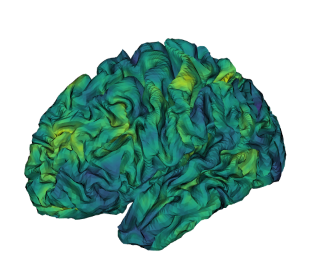
Despite its popularity, traditional fMRI analysis has some limitations, such as the fact that the data includes observations from many different tissue types, whereas it is known that neuronal activity only occurs in grey matter. Cortical surface fMRI (cs-fMRI) solves this problem by representing the cortical grey matter as a two-dimensional manifold surface (Fischl, 2012). The approach has recently grown in popularity because it also offers better visualisation, dimension reduction, and improved alignment of cortical areas across subjects. Furthermore, the manifold representation allows for more neurobiologically meaningful measures of distance between locations, which is of great importance for analysis. The main difficulty with analysing such data from a statistical point of view is that the spatial dependence across the cortical surface needs to be modelled. This difficulty was recently overcome by using the SPDE approach to define the first Bayesian GLM approach to cs-fMRI data (Mejia et al., 2020b) which has shown to be highly accurate compared to the standard GLM approach that ignores spatial dependence (Spencer et al., 2021). In Figure 1, we show a simulation of a Generalised Whittle–Matérn field on the cortical surface of a patient.
The models mentioned above are effective in finding which areas of the brain that are active when a particular task is being performed. Another way to study the brain, which recently has gained much attention, is to take a more holistic approach and to look at the functional organisation of the brain in the absence of a particular stimulus. A common method for this task is independent component analysis (ICA), which works reliably when looking at groups of patients (Calhoun et al., 2001). Performing estimation at a subject level is more challenging, and taking spatial dependence into account becomes more important at the subject level to reduce noise. This is again difficult to do for both fMRI and cs-fMRI data, but the SPDE approach has recently also facilitated the development of a spatial ICA method for the estimation of functional brain networks (Mejia et al., 2020a).
Similar techniques have also been applied to other anatomical manifolds, such as hearts. In order to model local activation times from electrograms, Coveney et al. (2020) estimated probabilistic activation times on a manifold of human atria. The triangulated manifold mesh was estimated from the measured individual, and then smoothed. The electrode positions were then projected to the nearest mesh point, and a the Kronecker product precision model from Section 4.3 used for the spatio-temporal activation process on the manifold, with the R-INLA software.
6.4 Seismology and material science
While the most common application of SPDE models in spatial statistics
is to 2-dimensional space, sometimes with added time, in seismology
the data and problems of interest are often 3-dimensional. The finite
element methods used in the Hilbert space construction works in the
same way for tetrahedralisations as it does for triangulations. This
was exploited by Zhang et al. (2016), to estimate seismic
velocity under the western USA down to 700 km depth. In this complex
inverse problem, they applied the SPDE models to both the sub-surface
velocity field, and to the seismic source and receiver fields on the
surface. They also provide a geometrical derivation of the finite
element matrices and for tetrahedral meshes, that
have since been implemented in an experimental R package at
https://github.com/finnlindgren/inlamesh3d.
Statistical modelling of porous materials is another application, on a very different spatial scale, that also requires models in 3-dimensional space. Barman and Bolin (2018) used the SPDE approach to design a model for the study of a porous ethylcellulose/hydroxypropylcellulose polymer blend that is used as a coating to control drug release from pharmaceutical tablets. This model has later been used to study how to pore geometry affects the diffusive transport through polymer films (Barman et al., 2019).
6.5 Point processes in ecology
One of the benefits of using local basis functions in SPDE constructions is the close resemblance to graph based Markov random field models that are common in ecology and epidemiology. This makes the step from aggregated counts on regions to continuous domain point process models very small. Direct approximation of inhomogeneous Poisson process likelihoods was analysed in detail by Simpson et al. (2016), and has since been automated as part of the inlabru software (Bachl et al., 2019; Yuan et al., 2017).
When is a linear predictor expression evaluated spatially, the inhomogeneous Poisson point process , , with intensity on a domain has log-likelihood
where the integral is a surface integral for manifold domains . The integral is in general intractable, but when is built from local basis functions as in Section 2.7, several options are available. For example, the discretisation , where are the mesh nodes and , provides a good and stable approximation. The resulting likelihood expression is not a Poisson model likelihood for since the two sums involve different spatial locations. However, it is similar enough that it is easy to implement in the R-INLA software, and to automate it, as in inlabru.
A key motivation for the inlabru software was to allow easier specification of models of this type, as well as more complex models, such as distance sampling from transect surveys, where the point process is only observed along lines, e.g. from a ship traversing the ocean. The surface integral is then effectively replaced by a line integral, and the probability of detecting a point (usually an animal or a group of animals) can also be incorporated. Such models however do not necessarily result in a log-linear expression with respect to the parameters of the intensity of the resulting thinned Poisson point process, . To deal with this, the inlabru method iteratively linearises the given predictor expression, and applies the INLA method for the linearised versions, until the posterior mode has been found.
Frequentist methods for distance sampling, that use penalised spline smoothers closely related to intrinsic stationary random field models, are available in the R package dsm (Miller et al., 2021).
7 Related methods
Here we highlight a few related or contrasting techniques and methods. Further connections, related and contrasting methods can be found in Cressie and Wikle (2011) and Wikle et al. (2019), that cover space-time models in the hierarchical model setting, and a variety of computational methods, including model assessment. The latter is becoming an increasingly important topic, since traditional basic measures such as the mean square error between the posterior mean (or frequentistic point estimate) only provide limited insights. In order to meaningfully compare complex spatial and spatio-temporal estimation techniques, it is essential to use comparison scores that take the estimated uncertainty of the predictions into account, such as log-density and log-probability scores (for continuous and discrete outcomes, respectively), CRPS (continuous ranked probability score), or Dawid-Sebastiani (the log-density score from the Gaussian distribution, which is a proper score with respect to the expectation and variance also for other distributions), see Gneiting and Raftery (2007). For the sparse precision matrices generated by the SPDE approach, leave-one-out cross validation (Vehtari et al., 2017) with such scores can also be applied (Ferkingstad et al., 2017).
7.1 Process priors versus smoothing penalties
The theory of reproducing kernel Hilbert spaces provide a close connection between frequentist penalised spline estimators and Bayesian Gaussian process priors, as was recently discussed by Miller et al. (2020). In parallel with the development of the stochastic PDE approaches, related development has been ongoing for PDE based penalties, addressing similar problems, such as complex shaped domains and non-Euclidean manifolds (Sangalli et al., 2013; Sangalli, 2021).
As alluded to in Section 2.2, a main difference between penalty minimisers (here usually the same as or similar to conditional expectations) and full stochastic processes, is that the penalty minimisers, associated with the same RKHS as the stochastic process, are fundamentally smoother than the process realisations. This also manifests in that for high dimensional Gaussian distributions (where random fields are at the extreme, infinite limit), the bulk of the probability mass lies far away from the expectation of the distribution, and this deviation is essential when quantifying prediction uncertainty. The variance of the point estimator or conditional expectation provided by a penalty method should not be confused with the prediction uncertainty provided by a full posterior distribution of the process.
7.2 Spectral model constructions and generalised Whittle-Matérn fields
An important aspect of using the Whittle SPDE is to generalise the Matérn covariance family to processes on manifolds, while keeping the local geometric interpretations. The SPDE generalisation of the Matérn covariance models to smooth manifolds retains all the differentiability and Markov subset properties of the original models, and are asymptotically equivalent for short range. The spectral representations are linked to the eigenfunctions and eigenvalues of the Laplacian and its manifold versions. The methods for fractional operators discussed in Section 4.1 have recently been extended using high order numerical methods for PDEs on Riemannian manifolds by Lang and Pereira (2021) and Harbrecht et al. (2021), involving polynomial and wavelet basis expansions. Other approaches to constructing valid models on spheres can be found in Porcu et al. (2016).
On , the eigenvalues of the Laplacian are for harmonic , , and on the sphere, is the eigenvalue for the spherical harmonic of order , . In the literature, spectral constructions are often used to define new families of models, e.g. for space-time models (Stein, 2005). When using the Whittle SPDE representation to generalise the Matérn models to the sphere and other non-Euclidean manifolds, the spectral representation of the Laplacian plays a key role. In contrast, the spherical covariance introduced by Guinness and Fuentes (2016) under the name Legendre-Matérn used in the spectrum definition instead of the that appears in the Whittle SPDE generalisation. In addition, the construction did not take into account the implications on the spectral representation of the model itself, leading to a different operator power, and lacking the factor from Section 2.5 in the spectrum-to-covariance transformation. Thus, where the Whittle-Matérn generalisation has , the Legendre-Matérn version has , which can not easily be reformulated using the eigenvalues of the Laplacian. These issues make that alternative generalisation of Matérn models less natural, as it loses all the Markov connections of the generalised Whittle representation, as well as the simple form of the precision operator, that can not be easily expressed via powers of the Laplacian. When only considering the theoretically valid expressions for positive definiteness, these kinds of effects are easily missed, and grounding more complex model construction in geometrical locally interpretable differential operators may provide better intuitive insight into the theory.
7.3 Global basis functions
In Section 2.7, locally supported basis functions were used in order to produce sparse precision matrices as well as retain this sparsity when conditioning on measurements. In the other extreme, global basis functions can be used, chosen so that the model precision for the basis weights are diagonal, but the posterior precisions generally dense. The Karhunen-Loève (K-L) expansion uses eigenfunctions of the covariance operator, or equivalently of the precision operator. The benefit of this type of finite dimensional spectral representation is that it results in a close approximation to the true covariance for a smaller number of basis functions. The main downside is the computational cost of evaluating the eigenfunctions, as these depend on the model parameters. Another choice is to use the eigenfunctions of the Laplacian that are involved in the Fourier-like spectral representations. These only depend on the shape of the domain, and can be calculated numerically at the start of the analysis (see Solin and Särkkä, 2020, for one such approach). However, since high frequencies may be needed to provide a good approximation of the true model, this approach is still expensive for general domains. In addition, the typical numerical solution is to use the same finite element methods to solve for the eigenvalues as is used to compute the entire conditional expectation. Hence, computing the eigenfunctions numerically is only helpful if they can then be used more effectively than the sparse precision matrices themselves. For both K-L and harmonic basis functions, the Hilbert space inner product yields diagonal prior precision matrices. The main problem in practical applications appear when the data structure does not admit efficient posterior distribution calculations due to the resulting dense precision matrices, due to the structure of the term in (11). This means that harmonic basis functions are mostly useful for very smooth fields that only need a few frequencies, or where fast Fourier transforms are possible.
When using spherical harmonics on the sphere, care must be taken when choosing a Legendre polynomial implementation, as some implementations are numerically unstable for orders above . For example, methods that first construct the polynomial coefficients explicitly, and then evaluate them, break down for orders above , including the implementations in the pracma and orthopolynom packages (Borchers, 2021; Novomestky, 2013). With these unstable implementations, the spatial resolution on the globe is limited to wavelengths of about degrees, or , making it unsuited for fine resolution problems such as the EUSTACE project discussed in Section 6.2. The GSL library implementation (Galassi, 2018; Hankin, 2006) however appears to be stable for much higher orders.
A numerical alternative is to compute the Laplacian eigenfunctions on a triangulation, via the generalised eigenvalue problem . This closely approximates the eigenfunctions of the continuous domain Laplacian, and works also on other manifolds than the sphere. This would be a slight modification of the directly graph based eigenfunctions used by Lee and Haran (2021).
7.4 Other precision approximation methods
Every computational approach to spatial processes can be viewed in (at least) to ways; as an approximation of a given model, or as a specially constructed model in itself. In the literature, both viewpoints are used, but since the structure of the approximations can be very specific to the details of the constructions, the second approach does not provide useful insights into the difference and similarities between the approaches. Instead, we find it more useful to take the first approach, and consider the continuous domain interpretability of the methods.
The Markov models resulting from the finite element Hilbert space approach to representing SPDE solutions has close links to several other methods for constructing computationally efficient approximations to given continuous domain models.
Just as one of the motivations for developing the SPDE/GMRF link in Lindgren et al. (2011) was to bridge the gap between discrete Markov models and continuous covariance models, there are further links between triangulation graphs for finite elements and other graph methods. Two recent examples are Sanz-Alonso and Yang (2021b) and Dunson et al. (2021), that construct different local Laplacian approximations on the same kind of graphs. The first of these two papers also show the extensive connections between the approaches, and how the finite element constructions provide better approximations to the continuous domain models, in the settings where they are available.
Another approach is the nearest neighbour Gaussian process (NNGP) construction from Datta et al. (2016), that takes a given covariance function and, in essence, constructs an incomplete Cholesky factorisation of the precision matrix for a given, ordered, sequence of spatial locations. By computing the exact conditional distribution given the previously included points, a discretised model is obtained. The benefit is that, instead of including the Cholesky infill that appears in the Cholesky factorisation of a Markovian precision matrix, only the previous neighbours are included. The downside is that the resulting representation depends on the order in which the spatial locations are included, which can lead to large discrepancies between the source covariance and the NNGP covariance. In contrast, for full Cholesky factorisations, the ordering of the nodes only affects the sparsity of the computed factorisation (Rue and Held, 2005). However, due to the relative speed of the NNGP construction, a potential extension could be to use the NNGP model as a fast preconditioner in large scale iterative solver methods. This would also be applicable to block-wise constructions, such as Katzfuss (2017); Quiroz et al. (2021); Peruzzi et al. (2020).
8 Discussion
After 10 years since the publication of Lindgren et al. (2011), the stochastic PDE method for constructing computationally efficient representations of spatial and spatio temporal Gaussian random fields has proven its value in a wide range of practical applications. There is now a wide variety in computational methods for spatial statistics, but many lack strong theoretical guarantees of fidelity in relation to desired continuous domain properties, or are limited to specific applications. In contrast, the SPDE approach exploits the close connections between different representations of Gaussian processes and their dependence structure, and the relative separation of the model construction itself from the computational methods, providing strong theoretical guarantees as well as efficient implementations. This has allowed Gaussian random field models to be incorporated in a variety of hierarchical models, and the method continues to be expanded to new application domains and more general dependency structures.
There is always a trade-off between generality and computational efficiency. The SPDE methods have the advantage that methods can be adapted from well-studied methods for deterministic PDE solvers, that are already capable of solving large systems. Part of the challenge is that the typical space-time precision operators for random fields are of much higher order than the typical ordinary Laplacian that is common in purely physics-motivated PDEs, which makes the standard preconditioning methods for iterative solvers inefficient. However, by exploiting local block structures, as well as multigrid methods and parallel solvers, these methods show great promise for even larger problems than can be solved with the current direct Cholesky methods, that are useable up to a few million elements; the largest single field solve in the EUSTACE project had nearly 2 million nodes.
Among the currently active areas of research are more general space-time extensions, non-stationarity and anisotropic models, and combinations thereof. We anticipate that this will serve to broaden the practical usefulness of SPDE models to realistic models for complex spatio-temporal data.
While it is still true that there is a practical implementation and preprocessing cost associated with the methods, and that this is true of all advanced spatial and spatio-temporal modelling techniques, the closing remark from Lindgren et al. (2011) that “such costs are unavoidable when efficient computations are required” is no longer as true now as it was in 2011, from the software users’ perspective. Interfaces such as inlabru are able to encapsulate all the internal bookkeeping and linear algebra in the internal code, allowing the software users to focus more on building structured and geometrically interpretable models.
Acknowledgements
As part of the EUSTACE project, Finn Lindgren received funding from the European Union’s “Horizon 2020 Programme for Research and Innovation”, under Grant Agreement no 640171.
References
- Aquino et al. (2021) Aquino, B., Castruccio, S., Gupta, V., Howard, S., 2021. Spatial modeling of mid-infrared spectral data with thermal compensation using integrated nested Laplace approximation. Appl. Opt. 60, 8609–8615. doi:10.1364/AO.435918.
- Asar et al. (2020) Asar, O., Bolin, D., Diggle, P.J., Wallin, J., 2020. Linear mixed effects models for non-Gaussian continuous repeated measurement data. J. R. Stat. Soc. Ser. C. Appl. Stat. 69, 1015–1065. doi:10.1111/rssc.12405. with discussion and a reply by the authors.
- Asri and Benamirouche (2021) Asri, A., Benamirouche, R., 2021. Using INLA/SPDE approach for estimating a spatial model for lung cancer mortality in Algeria 2016. Revue dÉconomie et de Statistique Appliquée 18, 261–277.
- Babyn et al. (2021) Babyn, J., Varkey, D., Regular, P., Ings, D., Mills Flemming, J., 2021. A Gaussian field approach to generating spatial age length keys. Fisheries Research 240, 105956. doi:10.1016/j.fishres.2021.105956.
- Bachl et al. (2019) Bachl, F.E., Lindgren, F., Borchers, D.L., Illian, J.B., 2019. inlabru: an R package for Bayesian spatial modelling from ecological survey data. Methods Ecol. Evol 10, 760–766. doi:10.1111/2041-210X.13168.
- Bakka (2019) Bakka, H., 2019. How to solve the stochastic partial differential equation that gives a Matérn random field using the finite element method. arXiv:1803.03765.
- Bakka et al. (2020) Bakka, H., Krainski, E., Bolin, D., Rue, H., Lindgren, F., 2020. The diffusion-based extension of the Matérn field to space-time. arXiv:2006.04917.
- Bakka et al. (2018) Bakka, H., Rue, H., Fuglstad, G.A., Riebler, A., Bolin, D., Illian, J., Krainski, E., Simpson, D., Lindgren, F., 2018. Spatial modelling with R-INLA: A review. Wiley Interdiscip. Rev. Comput. Stat. 10:e1443. doi:10.1002/wics.1443.
- Bakka et al. (2019) Bakka, H., Vanhatalo, J., Illian, J.B., Simpson, D., Rue, H., 2019. Non-stationary Gaussian models with physical barriers. Spat. Stat. 29, 268–288.
- Barman and Bolin (2018) Barman, S., Bolin, D., 2018. A three-dimensional statistical model for imaged microstructures of porous polymer films. J. Microsc. 269, 247–258. doi:10.1111/jmi.12623.
- Barman et al. (2019) Barman, S., Rootzén, H., Bolin, D., 2019. Prediction of diffusive transport through polymer films from characteristics of the pore geometry. AIChE Journal 65, 446–457.
- Bell et al. (2021) Bell, O., Jones, M.E., Cunningham, C.X., Ruiz-Aravena, M., Hamilton, D.G., Comte, S., Hamede, R.K., Bearhop, S., McDonald, R.A., 2021. Isotopic niche variation in Tasmanian devils Sarcophilus harrisii with progression of devil facial tumor disease. Ecology and Evolution 11, 8038–8053. doi:10.1002/ece3.7636.
- Beloconi et al. (2021) Beloconi, A., Probst-Hensch, N.M., Vounatsou, P., 2021. Spatio-temporal modelling of changes in air pollution exposure associated to the COVID-19 lockdown measures across Europe. Sci. Total Environ. 787, 147607. doi:10.1016/j.scitotenv.2021.147607.
- Berg et al. (2021) Berg, F., Shirajee, S., Folkvord, A., Godiksen, J.A., Skaret, G., Slotte, A., 2021. Early life growth is affecting timing of spawning in the semelparous Barents Sea capelin (Mallotus villosus). Prog. Oceanogr. 196, 102614. doi:10.1016/j.pocean.2021.102614.
- Bertozzi-Villa et al. (2021) Bertozzi-Villa, A., Bever, C.A., Koenker, H., Weiss, D.J., Vargas-Ruiz, C., Nandi, A.K., Gibson, H.S., Harris, J., Battle, K.E., Rumisha, S.F., Keddie, S., Amratia, P., Arambepola, R., Cameron, E., Chestnutt, E.G., Collins, E.L., Millar, J., Mishra, S., Rozier, J., Symons, T., Twohig, K.A., Hollingsworth, T.D., Gething, P.W., Bhatt, S., 2021. Maps and metrics of insecticide-treated net access, use, and nets-per-capita in Africa from 2000-2020. Nat. Commun. 12, 3589. doi:10.1038/s41467-021-23707-7.
- Besag (1974) Besag, J., 1974. Spatial Interaction and the Statistical Analysis of Lattice Systems. J. R. Stat. Soc. Ser. B Stat. Methodol. 36, 192–225. doi:10.1111/j.2517-6161.1974.tb00999.x.
- Besag and Kooperberg (1995) Besag, J., Kooperberg, C., 1995. On Conditional and Intrinsic Autoregression. Biometrika 82, 733–746. doi:10.2307/2337341.
- Besag and Mondal (2005) Besag, J., Mondal, D., 2005. First-Order Intrinsic Autoregressions and the De Wijs Process. Biometrika 92, 909–920. URL: https://www.jstor.org/stable/20441244.
- Bhatt et al. (2015) Bhatt, S., Weiss, D.J., Cameron, E., Bisanzio, D., Mappin, B., Dalrymple, U., Battle, K.E., Moyes, C.L., Henry, A., Eckhoff, P.A., Wenger, E.A., Briët, O., Penny, M.A., Smith, T.A., Bennett, A., Yukich, J., Eisele, T.P., Griffin, J.T., Fergus, C.A., Lynch, M., Lindgren, F., Cohen, J.M., Murray, C.L.J., Smith, D.L., Hay, S.I., Cibulskis, R.E., Gething, P.W., 2015. The effect of malaria control on Plasmodium falciparum in Africa between 2000 and 2015. Nature 526, 207–211. doi:10.1038/nature15535.
- Bleuel et al. (2021) Bleuel, J., Pennino, M., Longo, G., 2021. Coral distribution and bleaching vulnerability areas in Southwestern Atlantic under ocean warming. Scientific Reports 11, 12833. doi:10.1038/s41598-021-92202-2.
- Bolin (2012) Bolin, D., 2012. Models and Methods for Random Fields in Spatial Statistics with Computational Efficiency from Markov Properties. Ph.D. thesis. Faculty of Engineering, Centre for Mathematical Statistics, Lund University, Sweden.
- Bolin (2014) Bolin, D., 2014. Spatial Matérn fields driven by non-Gaussian noise. Scand. J. Stat. 41, 557–579. doi:10.1111/sjos.12046.
- Bolin and Kirchner (2020) Bolin, D., Kirchner, K., 2020. The rational SPDE approach for Gaussian random fields with general smoothness. J. Comp. Graph. Stat. 29, 274–285.
- Bolin and Kirchner (2021) Bolin, D., Kirchner, K., 2021. Equivalence of measures and asymptotically optimal linear prediction for gaussian random fields with fractional-order covariance operators. Preprint, arXiv:2101.07860.
- Bolin et al. (2018) Bolin, D., Kirchner, K., Kovács, M., 2018. Weak convergence of Galerkin approximations for fractional elliptic stochastic PDEs with spatial white noise. BIT 58, 881–906.
- Bolin et al. (2020) Bolin, D., Kirchner, K., Kovács, M., 2020. Numerical solution of fractional elliptic stochastic PDEs with spatial white noise. IMA J. Numer. Anal. 40, 1051–1073.
- Bolin and Lindgren (2011) Bolin, D., Lindgren, F., 2011. Spatial models generated by nested stochastic partial differential equations, with an application to global ozone mapping. Ann. Appl. Stat. 5, 523–550.
- Bolin and Lindgren (2013) Bolin, D., Lindgren, F., 2013. A comparison between Markov approximations and other methods for large spatial data sets. Comput. Statist. Data Anal. 61, 7–21. doi:10.1016/j.csda.2012.11.011.
- Bolin and Simas (2021) Bolin, D., Simas, A.B., 2021. R-INLA implementation of the covariance-based rational approximation. URL: https://davidbolin.github.io/rSPDE/articles/rspde_inla.html.
- Bolin and Wallin (2020) Bolin, D., Wallin, J., 2020. Multivariate type G Matérn stochastic partial differential equation random fields. J. R. Stat. Soc. Ser. B. Stat. Methodol. 82, 215–239.
- Bolin and Wallin (2021) Bolin, D., Wallin, J., 2021. Efficient methods for Gaussian Markov random fields under constraints, in: Advances in Neural Information Processing Systems 34, Curran Associates, Inc.. pp. 1–13.
- Boman et al. (2021) Boman, E.M., de Graaf, M., Kough, A.S., Izioka-Kuramae, A., Zuur, A.F., Smaal, A., Nagelkerke, L., 2021. Spatial dependency in abundance of Queen conch, Aliger gigas, in the Caribbean, indicates the importance of surveying deep-water distributions. Diversity and Distributions doi:10.1111/ddi.13392.
- Bonito and Pasciak (2015) Bonito, A., Pasciak, J.E., 2015. Numerical approximation of fractional powers of elliptic operators. Math. Comp. 84, 2083–2110.
- Borchers (2021) Borchers, H.W., 2021. pracma: Practical Numerical Math Functions. URL: https://CRAN.R-project.org/package=pracma. R package version 2.3.3.
- Borges da Silva et al. (2021) Borges da Silva, E.D., Xavier, A., Faria, M.V., 2021. Joint modeling of genetics and field variation in plant breeding trials using relationship and different spatial methods: A simulation study of accuracy and bias. Agronomy 11. doi:10.3390/agronomy11071397.
- Borovitskiy et al. (2020) Borovitskiy, V., Terenin, A., Mostowsky, P., Deisenroth, M.P., 2020. Matérn Gaussian processes on Riemannian manifolds. arXiv:2006.10160.
- Breivik et al. (2021) Breivik, O.N., Aanes, F., Søvik, G., Aglen, A., Mehl, S., Johnsen, E., 2021. Predicting abundance indices in areas without coverage with a latent spatio-temporal Gaussian model. ICES J. Mar. Sci. doi:10.1093/icesjms/fsab073.
- Calhoun et al. (2001) Calhoun, V.D., Adali, T., Pearlson, G.D., Pekar, J.J., 2001. A method for making group inferences from functional MRI data using independent component analysis. Human brain mapping 14, 140–151.
- Cameletti et al. (2013) Cameletti, M., Lindgren, F., Simpson, D., Rue, H., 2013. Spatio-temporal modeling of particulate matter concentration through the SPDE approach. Adv. Stat. Anal. 97, 109–131. doi:10.1007/s10182-012-0196-3.
- Carrizo Vergara et al. (2022) Carrizo Vergara, R., Allard, D., Dessasis, N., 2022. A general framework for SPDE-based stationary random fields. Bernoulli 28, 1–32. doi:10.3150/20-BEJ1317.
- Cavieres et al. (2021) Cavieres, J., Monnahan, C.C., Vehtari, A., 2021. Accounting for spatial dependence improves relative abundance estimates in a benthic marine species structured as a metapopulation. Fisheries Research 240, 105960. doi:10.1016/j.fishres.2021.105960.
- Cendoya et al. (2021) Cendoya, M., Hubel, A., Conesa, D., Vicent, A., 2021. Barrier effects on the spatial distribution of Xylella fastidiosa in Alicante, Spain. bioRxiv doi:10.1101/2021.04.01.438042.
- Chada et al. (2021) Chada, N.K., Roininen, L., Suuronen, J., 2021. Cauchy Markov random field priors for Bayesian inversion. Preprint, arXiv:2105.12488.
- Coveney et al. (2020) Coveney, S., Corrado, C., Roney, C.H., Wilkinson, R.D., Oakley, J.E., Lindgren, F., Williams, S.E., O’Neill, M.D., Niederer, S.A., Clayton, R.H., 2020. Probabilistic Interpolation of Uncertain Local Activation Times on Human Atrial Manifolds. IEEE Trans. Biomed. Eng. 67, 99–109. doi:10.1109/TBME.2019.2908486.
- Cox and Kirchner (2020) Cox, S.G., Kirchner, K., 2020. Regularity and convergence analysis in Sobolev and Hölder spaces for generalized Whittle–Matérn fields. Numer. Math. 146, 819–873.
- Cramér and Leadbetter (2004) Cramér, H., Leadbetter, M.R., 2004. Stationary and related stochastic processes. Dover Publications, Inc., Mineola, NY. Sample function properties and their applications, Reprint of the 1967 original.
- Cressie and Wikle (2011) Cressie, N., Wikle, C.K., 2011. Statistics for Spatio-Temporal Data. Wiley.
- Datta et al. (2016) Datta, A., Banerjee, S., Finley, A.O., Gelfand, A.E., 2016. Hierarchical Nearest-Neighbor Gaussian Process Models for Large Geostatistical Datasets. J. Amer. Statist. Assoc. 111, 800–812. doi:10.1080/01621459.2015.1044091.
- Dunson et al. (2021) Dunson, D.B., Wu, H.T., Wu, N., 2021. Graph based Gaussian processes on restricted domains. arXiv:2010.07242. accepted.
- Eidsvik et al. (2009) Eidsvik, J., Martino, S., Rue, H., 2009. Approximate Bayesian inference in spatial generalized linear mixed models. Scand. J. Stat. 36, 1–22.
- Eklund et al. (2016) Eklund, A., Nichols, T.E., Knutsson, H., 2016. Cluster failure: Why fMRI inferences for spatial extent have inflated false-positive rates. Proc. natl. acad. sci. 113, 7900–7905.
- Erisman and Tinney (1975) Erisman, A.M., Tinney, W.F., 1975. On computing certain elements of the inverse of a sparse matrix. Commun. ACM 18, 177–179.
- (53) Fecchio, A., Clark, N.J., Bell, J.A., Skeen, H.R., Lutz, H.L., De La Torre, G.M., Vaughan, J.A., Tkach, V.V., Schunck, F., Ferreira, F.C., Braga, E.M., Lugarini, C., Wamiti, W., Dispoto, J.H., Galen, S.C., Kirchgatter, K., Sagario, M.C., Cueto, V.R., González-Acuña, D., Inumaru, M., Sato, Y., Schumm, Y.R., Quillfeldt, P., Pellegrino, I., Dharmarajan, G., Gupta, P., Robin, V.V., Ciloglu, A., Yildirim, A., Huang, X., Chapa-Vargas, L., Álvarez-Mendizábal, P., Santiago-Alarcon, D., Drovetski, S.V., Hellgren, O., Voelker, G., Ricklefs, R.E., Hackett, S.J., Collins, M.D., Weckstein, J.D., Wells, K., . Global drivers of avian haemosporidian infections vary across zoogeographical regions. Global Ecology and Biogeography doi:10.1111/geb.13390.
- Ferkingstad et al. (2017) Ferkingstad, E., Held, L., Rue, H., 2017. Fast and accurate Bayesian model criticism and conflict diagnostics using R-INLA. Stat 6, 331–344. doi:10.1002/sta4.163.
- Fischl (2012) Fischl, B., 2012. Freesurfer. Neuroimage 62, 774–781.
- Florêncio et al. (2021) Florêncio, F.M., Alves, D.C., Lansac-Tôha, F.M., Silveira, M.J., Thomaz, S.M., 2021. The success of the invasive macrophyte Hydrilla verticillata and its interactions with the native Egeria najas in response to environmental factors and plant abundance in a subtropical reservoir. Aquatic Botany 175, 103432. doi:10.1016/j.aquabot.2021.103432.
- Friston et al. (1994) Friston, K.J., Holmes, A.P., Worsley, K.J., Poline, J.P., Frith, C.D., Frackowiak, R.S., 1994. Statistical parametric maps in functional imaging: a general linear approach. Human brain mapping 2, 189–210.
- Fuglstad et al. (2015a) Fuglstad, G.A., Lindgren, F., Simpson, D., Rue, H., 2015a. Exploring a New Class of Non-stationary Spatial {Gaussian} random fields with varying local anisotropy. Stat. Sin. 25, 115–133. URL: https://www.jstor.org/stable/24311007.
- Fuglstad et al. (2015b) Fuglstad, G.A., Simpson, D., Lindgren, F., Rue, H., 2015b. Does non-stationary spatial data always require non-stationary random fields? Spat. Stat. 14, 505–531. doi:10.1016/j.spasta.2015.10.001.
- Fuglstad et al. (2019) Fuglstad, G.A., Simpson, D., Lindgren, F., Rue, H., 2019. Constructing Priors that Penalize the Complexity of Gaussian Random Fields. J. Amer. Statist. Assoc. 114, 445–452. doi:10.1080/01621459.2017.1415907.
- Galassi (2018) Galassi, M.e.a., 2018. GNU Scientific Library reference manual. URL: https://www.gnu.org/software/gsl/.
- Ghattas and Willcox (2021) Ghattas, O., Willcox, K., 2021. Learning physics-based models from data: perspectives from inverse problems and model reduction. Acta Numerica 30, 445–554. doi:10.1017/S0962492921000064.
- Gneiting and Raftery (2007) Gneiting, T., Raftery, A.E., 2007. Strictly Proper Scoring Rules, Prediction, and Estimation. J. Amer. Statist. Assoc. 102, 359–378. doi:10.1198/016214506000001437.
- Gómez-Catasús et al. (2021) Gómez-Catasús, J., Barrero, A., Reverter, M., Bustillo-de la Rosa, D., Pérez-Granados, C., Traba, J., 2021. Landscape features associated to wind farms increase mammalian predator abundance and ground-nest predation. Biodivers. Conserv. 30, 2581–2604. doi:10.1007/s10531-021-02212-9.
- Griffiths and Lezama-Ochoa (2021) Griffiths, S.P., Lezama-Ochoa, N., 2021. A 40-year chronology of the vulnerability of spinetail devil ray (Mobula mobular) to eastern Pacific tuna fisheries and options for future conservation and management. Aquat. Conserv. doi:10.1002/aqc.3667.
- Guinness and Fuentes (2016) Guinness, J., Fuentes, M., 2016. Isotropic covariance functions on spheres: Some properties and modeling considerations. J. Multivar. Anal. 143, 143–152. doi:10.1016/j.jmva.2015.08.018.
- Hankin (2006) Hankin, R.K.S., 2006. Special functions in R: introducing the gsl package. R News 6.
- Harbrecht et al. (2021) Harbrecht, H., Herrmann, L., Kirchner, K., Schwab, C., 2021. Multilevel approximation of Gaussian random fields: Covariance compression, estimation and spatial prediction. Preprint, arXiv:2103.04424.
- Herrmann et al. (2020) Herrmann, L., Kirchner, K., Schwab, C., 2020. Multilevel approximation of Gaussian random fields: fast simulation. Math. Models Methods Appl. Sci. 30, 181–223.
- Hildeman et al. (2021) Hildeman, A., Bolin, D., Rychlik, I., 2021. Deformed SPDE models with an application to spatial modeling of significant wave height. Spat. Stat. 42, 100449.
- Hough et al. (2021) Hough, I., Sarafian, R., Shtein, A., Zhou, B., Lepeule, J., Kloog, I., 2021. Gaussian Markov random fields improve ensemble predictions of daily 1 km PM2.5 and pM10 across France. Atmos. Environ. 264, 118693. doi:10.1016/j.atmosenv.2021.118693.
- (72) Humphreys, J.M., Douglas, D.C., Ramey, A.M., Mullinax, J.M., Soos, C., Link, P., Walther, P., Prosser, D.J., . The spatial–temporal relationship of blue-winged teal to domestic poultry: Movement state modelling of a highly mobile avian influenza host. J. Appl. Ecol. doi:10.1111/1365-2664.13963.
- Ingebrigtsen et al. (2014) Ingebrigtsen, R., Lindgren, F., Steinsland, I., 2014. Spatial models with explanatory variables in the dependence structure. Spat. Stat. 8, 20–38. doi:10.1016/j.spasta.2013.06.002.
- Jarvis et al. (2021) Jarvis, J.C., McKenna, S.A., Rahseed, M.A., 2021. Seagrass seed bank spatial structure and function following a large-scale decline. Mar. Ecol. Prog. Ser. 665, 75–87. doi:10.3354/meps13668.
- Katzfuss (2017) Katzfuss, M., 2017. A Multi-Resolution Approximation for Massive Spatial Datasets. J. Amer. Statist. Assoc. 112, 201–214. doi:10.1080/01621459.2015.1123632.
- Khristenko et al. (2019) Khristenko, U., Scarabosio, L., Swierczynski, P., Ullmann, E., Wohlmuth, B., 2019. Analysis of boundary effects on PDE-based sampling of Whittle-Matérn random fields. SIAM/ASA J. Uncertain. Quantif. 7, 948–974. doi:10.1137/18M1215700.
- Kimeldorf and Wahba (1970) Kimeldorf, G.S., Wahba, G., 1970. A Correspondence Between Bayesian Estimation on Stochastic Processes and Smoothing by Splines. Ann. Math. Stat. 41, 495–502. URL: https://www.jstor.org/stable/2239347.
- Kirchner and Bolin (2021) Kirchner, K., Bolin, D., 2021. Necessary and sufficient conditions for asymptotically optimal linear prediction of random fields on compact metric spaces. Ann. Stat. To appear.
- Knorr-Held and Rue (2002) Knorr-Held, L., Rue, H., 2002. On block updating in Markov random field models for disease mapping. Scand. J. Stat. 29, 597–614.
- Krainski et al. (2018) Krainski, E.T., Gómez-Rubio, V., Bakka, H., Lenzi, A., Castro-Camilio, D., Simpson, D., Lindgren, F., Rue, H., 2018. Advanced Spatial Modeling with Stochastic Partial Differential Equations using R and INLA. CRC press. Gitbook version https://becarioprecario.bitbucket.io/spde-gitbook/.
- Lang and Pereira (2021) Lang, A., Pereira, M., 2021. Galerkin–Chebyshev approximation of Gaussian random fields on compact Riemannian manifolds. arXiv:2107.02667.
- Lang and Schwab (2015) Lang, A., Schwab, C., 2015. Isotropic Gaussian random fields on the sphere: regularity, fast simulation and stochastic partial differential equations. Ann. Appl. Probab. 25, 3047–3094. doi:10.1214/14-AAP1067.
- Lauritzen (1996) Lauritzen, S.L., 1996. Graphical Models. volume 17 of Oxford Statistical Science Series. The Clarendon Press Oxford University Press, New York. Oxford Science Publications.
- Lee et al. (2021) Lee, B., Arkhipkin, A., Randhawa, H.S., 2021. Environmental drivers of Patagonian toothfish (Dissostichus eleginoides) spatial-temporal patterns during an ontogenetic migration on the Patagonian Shelf. Estuar. Coast. Shelf Sci. 259, 107473. doi:10.1016/j.ecss.2021.107473.
- Lee and Haran (2021) Lee, B.S., Haran, M., 2021. PICAR: An efficient extendable approach for fitting hierarchical spatial models. Technometrics 0, 1–12. doi:10.1080/00401706.2021.1933596.
- Levis et al. (2021) Levis, A., Lee, D., Tropp, J.A., Gammie, C.F., Bouman, K.L., 2021. Inference of black hole fluid-dynamics from sparse interferometric measurements. Proceedings of IEEE International Conference on Computer Vision 2021 To appear.
- Li (2021) Li, D., 2021. Urban planning image feature enhancement and simulation based on partial differential equation method. Adv. Math. Phys. 2021, 1700287. doi:10.1155/2021/1700287.
- (88) Lindenmayer, D., Taylor, C., Blanchard, W., . Empirical analyses of the factors influencing fire severity in southeastern Australia. Ecosphere 12, e03721. doi:10.1002/ecs2.3721.
- Lindgren and Rue (2008) Lindgren, F., Rue, H., 2008. A note on the second order random walk model for irregular locations. Scand. J. Stat. 35, 691–700.
- Lindgren and Rue (2015) Lindgren, F., Rue, H., 2015. Bayesian spatial modelling with R-INLA. J. Stat. Softw. 63, 1–25.
- Lindgren et al. (2011) Lindgren, F., Rue, H., Lindström, J., 2011. An explicit link between Gaussian fields and Gaussian Markov random fields: the stochastic partial differential equation approach. J. R. Stat. Soc. Ser. B Stat. Methodol. 73, 423–498. With discussion and a reply by the authors.
- Lindgren (2012) Lindgren, G., 2012. Stationary Stochastic Processes: Theory and Applications. CRC Press, Chapman and Hall.
- Liu et al. (2016) Liu, X., Guillas, S., Lai, M.J., 2016. Efficient Spatial Modeling Using the SPDE Approach With Bivariate Splines. J. Comp. Graph. Stat. 25, 1176–1194. doi:10.1080/10618600.2015.1081597.
- Mannseth et al. (2021) Mannseth, J., Berentsen, G.D., Skaug, H.J., Lie, R.T., Moster, D., 2021. Variation in use of Caesarean section in Norway: An application of spatio-temporal Gaussian random fields. Scand. J. Public Health doi:10.1177/140349482008579.
- Martino et al. (2021) Martino, S., Pace, D.S., Moro, S., Casoli, E., Ventura, D., Frachea, A., Silvestri, M., Arcangeli, A., Giacomini, G., Ardizzone, G., Lasinio, G.J., 2021. Integration of presence-only data from several sources. a case study on dolphins’ spatial distribution. arXiv:2103.16125.
- Martins et al. (2013) Martins, T.G., Simpson, D., Lindgren, F., Rue, H., 2013. Bayesian computing with INLA: New features. Comput. Statist. Data Anal. 67, 68–83.
- Matérn (1960) Matérn, B., 1960. Spatial variation: Stochastic models and their application to some problems in forest surveys and other sampling investigations. Meddelanden Från Statens Skogsforskningsinstitut, Band 49, Nr. 5, Stockholm.
- Maynou et al. (2021) Maynou, L., Monfort, M., Morley, B., Ordóñez, J., 2021. Club convergence in European housing prices: The role of macroeconomic and housing market fundamentals. Economic Modelling 103, 105595. doi:10.1016/j.econmod.2021.105595.
- Mejia et al. (2020a) Mejia, A.F., Bolin, D., Yue, Y.R., Wang, J., Caffo, B.S., Nebel, M.B., 2020a. A spatial template independent component analysis model for subject-level brain network estimation and inference. arXiv preprint arXiv:2005.13388 .
- Mejia et al. (2020b) Mejia, A.F., Yue, Y., Bolin, D., Lindgren, F., Lindquist, M.A., 2020b. A Bayesian general linear modeling approach to cortical surface fMRI data analysis. J. Amer. Statist. Assoc. 115, 501–520. doi:10.1080/01621459.2019.1611582.
- Miller et al. (2020) Miller, D.L., Glennie, R., Seaton, A.E., 2020. Understanding the Stochastic Partial Differential Equation Approach to Smoothing. J. Agric. Biol. Environ. Stat. 25, 1–16. doi:10.1007/s13253-019-00377-z.
- Miller et al. (2021) Miller, D.L., Rexstad, E., Burt, L., Bravington, M.V., Hedley., S., 2021. dsm: Density Surface Modelling of Distance Sampling Data. URL: https://CRAN.R-project.org/package=dsm. R package version 2.3.1.
- Monnahan et al. (2021) Monnahan, C.C., Thorson, J.T., Kotwicki, S., Lauffenburger, N., Ianelli, J.N., Punt, A.E., 2021. Incorporating vertical distribution in index standardization accounts for spatiotemporal availability to acoustic and bottom trawl gear for semi-pelagic species. ICES J. Mar. Sci. 78, 1826–1839. doi:10.1093/icesjms/fsab085.
- Moraga et al. (2021) Moraga, P., Dean, C., Inoue, J., Morawiecki, P., Noureen, S.R., Wang, F., 2021. Bayesian spatial modelling of geostatistical data using INLA and SPDE methods: A case study predicting malaria risk in Mozambique. Spat. Spatio-temporal Epidemiol. 39, 100440. doi:10.1016/j.sste.2021.100440.
- Morales and Laurini (2021) Morales, A.B., Laurini, M.P., 2021. Firm location: A spatial point process approach. Appl. Spat. Anal. Policy doi:10.1007/s12061-021-09419-x.
- Moses et al. (2021) Moses, J., Aheto, K., Dagne, G.A., 2021. Geostatistical analysis, web-based mapping, and environmental determinants of under-5 stunting: evidence from the 2014 Ghana Demographic and Health Survey. The Lancet Planetary Health 5, e347–e355. doi:10.1016/S2542-5196(21)00080-2.
- Novomestky (2013) Novomestky, F., 2013. orthopolynom: Collection of functions for orthogonal and orthonormal polynomials. URL: https://CRAN.R-project.org/package=orthopolynom. R package version 1.0-5.
- Nychka et al. (2016) Nychka, D., Hammerling, D., Sain, S., Lenssen, N., 2016. LatticeKrig: Multiresolution Kriging based on Markov random fields. doi:10.5065/D6HD7T1R. R package version 8.4.
- Peruzzi et al. (2020) Peruzzi, M., Banerjee, S., Finley, A.O., 2020. Highly Scalable Bayesian Geostatistical Modeling via Meshed Gaussian Processes on Partitioned Domains. J. Amer. Statist. Assoc. 0, 1–14. doi:10.1080/01621459.2020.1833889.
- Porcu et al. (2016) Porcu, E., Bevilacqua, M., Genton, M.G., 2016. Spatio-Temporal Covariance and Cross-Covariance Functions of the Great Circle Distance on a Sphere. J. Amer. Statist. Assoc. 111, 888–898. doi:10.1080/01621459.2015.1072541.
- Quiroz et al. (2021) Quiroz, Z.C., Prates, M.O., Dey, D.K., Rue, H., 2021. Fast Bayesian inference of block nearest neighbor Gaussian process for large data. arXiv:1908.06437.
- Rayner et al. (2020) Rayner, N.A., Auchmann, R., Bessembinder, J., Brönnimann, S., Brugnara, Y., Capponi, F., Carrea, L., Dodd, E.M.A., Ghent, D., Good, E., Høyer, J.L., Kennedy, J.J., Kent, E.C., Killick, R.E., Linden, P.v.d., Lindgren, F., Madsen, K.S., Merchant, C.J., Mitchelson, J.R., Morice, C.P., Nielsen-Englyst, P., Ortiz, P.F., Remedios, J.J., Schrier, G.v.d., Squintu, A.A., Stephens, A., Thorne, P.W., Tonboe, R.T., Trent, T., Veal, K.L., Waterfall, A.M., Winfield, K., Winn, J., Woolway, R.I., 2020. The EUSTACE Project: Delivering Global, Daily Information on Surface Air Temperature. Bull. Am. Meteorol. Soc. 101, E1924–E1947. doi:10.1175/BAMS-D-19-0095.1.
- Roininen et al. (2019) Roininen, L., Girolami, M., Lasanen, S., Markkanen, M., 2019. Hyperpriors for Matérn fields with applications in Bayesian inversion. Inverse Probl. Imaging 13, 1–29. doi:10.3934/ipi.2019001.
- Roininen et al. (2014) Roininen, L., Huttunen, J.M.J., Lasanen, S., 2014. Whittle-Matérn priors for Bayesian statistical inversion with applications in electrical impedance tomography. Inverse Probl. Imaging 8, 561–586. doi:10.3934/ipi.2014.8.561.
- Roininen et al. (2018) Roininen, L., Lasanen, S., Orispää, M., Särkkä, S., 2018. Sparse Approximations of Fractional Matérn Fields. Scand. J. Stat. 45, 194–216. doi:10.1111/sjos.12297.
- Roksvåg et al. (2021) Roksvåg, T., Steinsland, I., Engeland, K., 2021. A two-field geostatistical model combining point and areal observations–A case study of annual runoff predictions in the Voss area. J. R. Stat. Soc. Ser. C. Appl. Stat. 70, 934–960. doi:10.1111/rssc.12492.
- Roksvåg et al. (2021) Roksvåg, T., Steinsland, I., Engeland, K., 2021. Estimating mean annual runoff by using a geostatistical spatially varying coefficient model that incorporates process-based simulations and short records, in: EGU General Assembly Conference Abstracts, pp. EGU21–4233.
- Rozanov (1977) Rozanov, J.A., 1977. Markov random fields and stochastic partial differential equations. Sbornik: Mathematics 32, 515–534.
- Rue and Held (2005) Rue, H., Held, L., 2005. Gaussian Markov Random Fields: Theory and Applications. volume 104 of Monographs on Statistics and Applied Probability. Chapman & Hall, London. doi:10.1201/9780203492024.
- Rue and Held (2010) Rue, H., Held, L., 2010. Markov random fields, in: Gelfand, A., Diggle, P., Fuentes, M., Guttorp, P. (Eds.), Handbook of Spatial Statistics. CRC/Chapman & Hall, Boca Raton, FL, pp. 171–200.
- Rue and Martino (2007) Rue, H., Martino, S., 2007. Approximate Bayesian inference for hierarchical Gaussian Markov random fields models. J. Stat. Plan. Inference 137, 3177–3192. Special Issue: Bayesian Inference for Stochastic Processes.
- Rue et al. (2009) Rue, H., Martino, S., Chopin, N., 2009. Approximate Bayesian inference for latent Gaussian models using integrated nested Laplace approximations. J. R. Stat. Soc. Ser. B Stat. Methodol. 71, 319–392. With discussion and a reply by the authors.
- Rue et al. (2017) Rue, H., Riebler, A., Sørbye, S.H., Illian, J.B., Simpson, D.P., Lindgren, F.K., 2017. Bayesian computing with INLA: A review. Annu. Rev. Stat. Appl. 4, 395–421. doi:10.1146/annurev-statistics-060116-054045.
- Sampson and Guttorp (1992) Sampson, P.D., Guttorp, P., 1992. Nonparametric Estimation of Nonstationary Spatial Covariance Structure. J. Amer. Statist. Assoc. 87, 108–119. doi:10.2307/2290458.
- Sangalli (2021) Sangalli, L.M., 2021. Spatial regression with partial differential equation regularisation. Int. Stat. Rev. doi:10.1111/insr.12444.
- Sangalli et al. (2013) Sangalli, L.M., Ramsay, J.O., Ramsay, T.O., 2013. Spatial spline regression models. J. R. Stat. Soc. Ser. B. Stat. Methodol. 75, 681–703. doi:10.1111/rssb.12009.
- Sanz-Alonso and Yang (2021a) Sanz-Alonso, D., Yang, R., 2021a. Finite element representations of Gaussian processes: Balancing numerical and statistical accuracy. arXiv:2109.02777.
- Sanz-Alonso and Yang (2021b) Sanz-Alonso, D., Yang, R., 2021b. The SPDE approach to Matérn fields: Graph representations. Stat. Sci. , 1–53Accepted.
- Schoenberg (1942) Schoenberg, I.J., 1942. Positive definite functions on spheres. Duke Math. J. 9, 96–108. doi:10.1215/S0012-7094-42-00908-6.
- Scott (2021) Scott, R.P., 2021. Shared streets, park closures and environmental justice during a pandemic emergency in Denver, Colorado. J. Trans. Health 21, 101075. doi:10.1016/j.jth.2021.101075.
- Sicacha-Parada et al. (2021) Sicacha-Parada, J., Pavon-Jordan, D., Steinsland, I., May, R., Stokke, B., Øien, I.J., 2021. A spatial modeling framework for monitoring surveys with different sampling protocols with a case study for bird populations in mid-Scandinavia. arXiv:2104.05751.
- Sidén et al. (2021) Sidén, P., Lindgren, F., Bolin, D., Eklund, A., Villani, M., 2021. Spatial 3D Matérn priors for fast whole-brain fMRI analysis. Bayesian Anal. , 1–28doi:10.1214/21-BA1283.
- Simpson et al. (2016) Simpson, D., Illian, J.B., Lindgren, F., Sørbye, S.H., Rue, H., 2016. Going off grid: computationally efficient inference for log-Gaussian Cox processes. Biometrika 103, 49–70. doi:10.1093/biomet/asv064.
- Simpson et al. (2012a) Simpson, D., Lindgren, F., Rue, H., 2012a. In order to make spatial statistics computationally feasible, we need to forget about the covariance function. Environmetrics 23, 65–74. doi:10.1002/env.1137.
- Simpson et al. (2012b) Simpson, D., Lindgren, F., Rue, H., 2012b. Think continuous: Markovian Gaussian models in spatial statistics. Spat. Stat. 1, 16–29. doi:10.1016/j.spasta.2012.02.003.
- Simpson et al. (2017) Simpson, D.P., Rue, H., Riebler, A., Martins, T.G., Sørbye, S.H., 2017. Penalising model component complexity: A principled, practical approach to constructing priors (with discussion). Stat. Sci. 32, 1–28.
- Solin and Särkkä (2020) Solin, A., Särkkä, S., 2020. Hilbert space methods for reduced-rank Gaussian process regression. Stat. Comput. 30, 419–446. doi:10.1007/s11222-019-09886-w.
- Spencer et al. (2021) Spencer, D., Yue, Y.R., Bolin, D., Ryan, S., Mejia, A.F., 2021. Spatial Bayesian GLM on the cortical surface produces reliable task activations in individuals and groups. arXiv:2106.06669.
- Stein (1999) Stein, M.L., 1999. Interpolation of Spatial Data: Some Theory for Kriging. Springer Series in Statistics, Springer-Verlag, New York.
- Stein (2005) Stein, M.L., 2005. Space–time covariance functions. J. Amer. Statist. Assoc. 100, 310–321.
- Särkkä et al. (2013) Särkkä, S., Solin, A., Hartikainen, J., 2013. Spatiotemporal Learning via Infinite-Dimensional Bayesian Filtering and Smoothing: A Look at Gaussian Process Regression Through Kalman Filtering. IEEE Signal Process. Mag. 30, 51–61. doi:10.1109/MSP.2013.2246292.
- Sørbye et al. (2019) Sørbye, S.H., Myrvoll-Nilsen, E., Rue, H., 2019. An approximate fractional Gaussian noise model with O(n) computational cost. Stat. Comput. 29, 821–833. doi:10.1007/s11222-018-9843-1.
- Takahashi et al. (1973) Takahashi, K., Fagan, J., Chen, M.S., 1973. Formation of a sparse bus impedance matrix and its application to short circuit study, in: 8th PICA Conference proceedings, IEEE Power Engineering Society. pp. 63–69. Papers presented at the Power Industry Computer Application Conference in Minneapolis, Minnesota.
- Taylor et al. (2021) Taylor, C., Blanchard, W., Lindenmayer, D.B., 2021. What are the associations between thinning and fire severity? Austral Ecology 46, 145–1439. doi:10.1111/aec.13096.
- Thorson et al. (2021) Thorson, J.T., Barbeaux, S.J., Goethel, D.R., Kearney, K.A., Laman, E.A., Nielsen, J.K., Siskey, M.R., Siwicke, K., Thompson, G.G., 2021. Estimating fine-scale movement rates and habitat preferences using multiple data sources. Fish and Fisheries 22, 1359–1376. doi:10.1111/faf.12592.
- Valente and Laurini (2021a) Valente, F., Laurini, M., 2021a. Pre-harvest sugarcane burning: A statistical analysis of the environmental impacts of a regulatory change in the energy sector. Cleaner Engineering and Technology 4, 100255. doi:10.1016/j.clet.2021.100255.
- Valente and Laurini (2021b) Valente, F., Laurini, M., 2021b. Spatio-temporal analysis of fire occurrence in Australia. Stochastic Environmental Research and Risk Assessment 35, 1759–1770. doi:10.1007/s00477-021-02043-8.
- van Niekerk et al. (2021) van Niekerk, J., Bakka, H., Rue, H., Schenk, O., 2021. New frontiers in Bayesian modeling using the INLA package in R. J. Stat. Softw. 100, 1–28. doi:10.18637/jss.v100.i02.
- van Woesik and Cacciapaglia (2021) van Woesik, R., Cacciapaglia, C.W., 2021. Thermal stress jeopardizes carbonate production of coral reefs across the western and central Pacific Ocean. PLOS ONE 16, 1–18. doi:10.1371/journal.pone.0249008.
- Vandeskog et al. (2021a) Vandeskog, S.M., Martino, S., Castro-Camilo, D., Rue, H., 2021a. Modelling short-term precipitation extremes with the blended generalised extreme value distribution. arXiv:2105.09062.
- Vandeskog et al. (2021b) Vandeskog, S.M., Thorarinsdottir, T.L., Steinsland, I., Lindgren, F., 2021b. Quantile based modelling of diurnal temperature range with the five-parameter lambda distribution. arXiv:2109.11180.
- Vehtari et al. (2017) Vehtari, A., Gelman, A., Gabry, J., 2017. Practical Bayesian model evaluation using leave-one-out cross-validation and WAIC. Stat. Comput. 27, 1413–1432. doi:10.1007/s11222-016-9696-4.
- Vogel et al. (2021) Vogel, E.F., Biuw, M., Blanchet, M.A., Jonsen, I.D., Mul, E., Johnsen, E., Hjøllo, S.S., Olsen, M.T., Dietz, R., Rikardsen, A., 2021. Killer whale movements on the Norwegian shelf are associated with herring density. Marine Ecology Progress Series 665, 217–231. doi:10.3354/meps13685.
- Wahba (1981) Wahba, G., 1981. Spline Interpolation and Smoothing on the Sphere. SIAM J. Sci. Statist. Comput. 2, 5–16. doi:10.1137/0902002.
- Walder and Hanks (2020) Walder, A., Hanks, E.M., 2020. Bayesian analysis of spatial generalized linear mixed models with Laplace moving average random fields. Comput. Statist. Data Anal. 144, 106861, 13. doi:10.1016/j.csda.2019.106861.
- Wallin and Bolin (2015) Wallin, J., Bolin, D., 2015. Geostatistical modelling using non-Gaussian Matérn fields. Scand. J. Stat. 42, 872–890. doi:10.1111/sjos.12141.
- Wang and Zuo (2021) Wang, J., Zuo, R., 2021. Spatial modelling of hydrothermal mineralization-related geochemical patterns using INLA+SPDE and local singularity analysis. Comput. Geosci. 154, 104822. doi:10.1016/j.cageo.2021.104822.
- Whittle (1954) Whittle, P., 1954. On stationary processes in the plane. Biometrika 41, 434–449. doi:10.1093/biomet/41.3-4.434.
- Whittle (1963) Whittle, P., 1963. Stochastic processes in several dimensions. Bull. Internat. Statist. Inst. 40, 974–994.
- Wikle et al. (2019) Wikle, C.K., Zammit-Mangion, A., Cressie, N., 2019. Spatio-Temporal Statistics with R. Chapman & Hall/CRC, Boca Raton, FL.
- Williamson et al. (2021) Williamson, L.D., Scott, B.E., Laxton, M.R., Bachl, F.E., Illian, J.B., Brookes, K.L., Thompson, P.M., 2021. Spatiotemporal variation in harbor porpoise distribution and foraging across a landscape of fear. Marine Mammal Science , 1–16doi:10.1111/mms.12839.
- Wright et al. (2021) Wright, N., Newell, K., Lam, K.B.H., Kurmi, O., Chen, Z., Kartsonaki, C., 2021. Estimating ambient air pollutant levels in Suzhou through the SPDE approach with R-INLA. Int. J. Hyg. Environ. Health 235, 113766. doi:10.1016/j.ijheh.2021.113766.
- Xi et al. (2021) Xi, C., Wu, Z., Qian, T., Liu, L., Wang, J., 2021. A Bayesian model for estimating the effects of human disturbance on wildlife habitats based on nighttime light data and INLA-SPDE. Appl. Spat. Anal. Policy doi:10.1007/s12061-021-09402-6.
- Yuan et al. (2017) Yuan, Y., Bachl, F.E., Lindgren, F., Borchers, D.L., Illian, J.B., Buckland, S.T., Rue, H., Gerrodette, T., 2017. Point process models for spatio-temporal distance sampling data from a large-scale survey of blue whales. Ann. Appl. Stat. 11, 2270–2297. doi:10.1214/17-AOAS1078.
- Yue et al. (2014) Yue, Y.R., Simpson, D., Lindgren, F., Rue, H., 2014. Bayesian adaptive smoothing spline using stochastic differential equations. Bayesian Anal. 9, 397–424.
- Zhang (2004) Zhang, H., 2004. Inconsistent estimation and asymptotically equal interpolations in model-based geostatistics. J. Amer. Statist. Assoc. 99, 250–261.
- Zhang et al. (2021) Zhang, H., Guilleminot, J., Gomez, L.J., 2021. Stochastic modeling of geometrical uncertainties on complex domains, with application to additive manufacturing and brain interface geometries. Comput. Methods Appl. Mech. Eng. 385, 114014. doi:10.1016/j.cma.2021.114014.
- Zhang et al. (2016) Zhang, R., Czado, C., Sigloch, K., 2016. Bayesian spatial modelling for high dimensional seismic inverse problems. J. R. Stat. Soc. Ser. C. Appl. Stat. 65, 187–213. URL: https://www.jstor.org/stable/24772417.
Appendix A Reproducing kernel Hilbert space connection details
As in Section 2.2, let be the adjoint of , i.e. an operator such that on the manifold domain , and also assume that is invertible. Also let be a standard Gaussian white noise process on , and let be a solution to with covariance function . Then, by construction,
| (13) |
so that
where the subscript notation and is used to indicate which spatial variable is operated on. Since the equality holds for all admissible and , this shows that
where is a Dirac delta. Define . Then, for all and all suitable ,
| (14) | ||||
which shows that this is the inner product for the RKHS for the covariance that is associated with the covariance product in (13). By taking we obtain the kernel reproducing property . The derivation (14) directly shows that , which means that the covariance function is a Green’s function of the precision operator . After a change of test functions in (13), we can also write .