Periodic Fast Multipole Method

Abstract

A new scheme is presented for imposing periodic boundary conditions on unit cells with arbitrary source distributions. We restrict our attention here to the Poisson, modified Helmholtz, Stokes and modified Stokes equations. The approach extends to the oscillatory equations of mathematical physics, including the Helmholtz and Maxwell equations, but we will address these in a companion paper, since the nature of the problem is somewhat different and includes the consideration of quasiperiodic boundary conditions and resonances. Unlike lattice sum-based methods, the scheme is insensitive to the unit cell’s aspect ratio and is easily coupled to adaptive fast multipole methods (FMMs). Our analysis relies on classical “plane-wave” representations of the fundamental solution, and yields an explicit low-rank representation of the field due to all image sources beyond the first layer of neighboring unit cells. When the aspect ratio of the unit cell is large, our scheme can be coupled with the nonuniform fast Fourier transform (NUFFT) to accelerate the evaluation of the induced field. Its performance is illustrated with several numerial examples.

1 Introduction

Applications in electrostatics, magnetostatics, fluid mechanics, and elasticity often involve sources contained in a unit cell $\mathcal{C}$, centered at the origin, on which are imposed periodic boundary conditions. In two dimensions, such a unit cell is defined by two fundamental translation vectors ${\hat{\bf e}}_{1}$ and ${\hat{\bf e}}_{2}$. In the doubly periodic setting, we assume (without loss of generalilty) that $\|{\hat{\bf e}}_{1}\|\geq\|{\hat{\bf e}}_{2}\|$ and that, by a suitable rotation, ${\hat{\bf e}}_{1}$ is aligned with the $x$-axis and ${\hat{\bf e}}_{2}$ lies in the upper half space (see Figure 1). That is, we let $\mathcal{C}=\left\{x_{1}{\hat{\bf e}}_{1}+x_{2}{\hat{\bf e}}_{2}\in\mathbb{R}^{2}|\ x_{1},x_{2}\in[-\frac{1}{2},\frac{1}{2}]\right\}$, where ${\hat{\bf e}}_{1}=\langle d,0\rangle$, ${\hat{\bf e}}_{2}=\langle\xi,\eta\rangle$, with $d,\eta>0$ and $d\geq\sqrt{\xi^{2}+\eta^{2}}$. In the singly periodic setting, we assume that the periodic direction is aligned with the $x$-axis, but can no longer assume that $\|{\hat{\bf e}}_{1}\|\geq\|{\hat{\bf e}}_{2}\|$. Without loss of generality, however, we can assume that the unit cell is rectangular (Figure 1) and of dimension $d\times\eta$. Letting ${\bf t}=(x,y)$ and letting $u({\bf t})$ denote a scalar quantity of interest, by doubly periodic boundary conditions we mean that $u({\bf t})$ must satisfy:

$$u({\bf t}+{\hat{\bf e}}_{1}) =u({\bf t}),$$ (1)

$$u({\bf t}+{\hat{\bf e}}_{2}) =u({\bf t}).$$

By singly periodic boundary conditions we mean that $u({\bf t})$ must satisfy:

$$u({\bf t}+{\hat{\bf e}}_{1}) =u({\bf t}),$$ (2)

and a standard outgoing/decay condition in the $y$-direction.

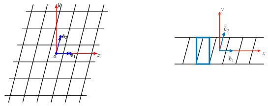
Figure 1: In the doubly periodic case (left), the unit cell is a parallelogram which tiles the entire plane. By convention, we assume that the lattice is oriented so that the longer cell dimension is aligned with the $x$-axis: $\|{\hat{\bf e}}_{1}\|\geq\|{\hat{\bf e}}_{2}\|$. In the singly periodic case (right), we assume the periodic direction is aligned with the $x$-axis. The unit cell may still be a parallelogram, but we can always define a corresponding rectangular unit cell, indicated by thick blue lines. In this case, we cannot assume that the long cell dimension is aligned with the $x$-axis. Periodic boundary conditions are imposed through the method of images: that is, by including the influence of the translated sources in every image cell on the targets in the fundamental unit cell.

For the moment, let us assume that the governing partial differential equation (PDE) is

$$\Delta u({\bf t})-\beta^{2}u({\bf t})=\sum_{j=1}^{N_{S}}q_{j}\delta({\bf t}-{\bf s}_{j}),$$ (3)

with $\beta$ real and non-negative. Here, ${\bf t},{\bf s}_{j}$ are points lying within the unit cell $\mathcal{C}$. We refer to (3) as the modified Helmholtz equation when $\beta>0$. When $\beta=0$, of course, we obtain the Poisson equation. In two dimensions, the free-space Green’s functions for these equations are well-known and given by [35, 41]

$$G({\bf t},{\bf s})=\frac{1}{2\pi}K_{0}(\beta\|{\bf t}-{\bf s}\|),\quad G({\bf t},{\bf s})=\frac{1}{2\pi}\log(1/\|{\bf t}-{\bf s}\|),$$

respectively, where $K_{0}$ denotes the zeroth order modified Bessel function of the second kind [38].

Thus, in free space, the solution to (3) at targets ${\bf t}_{1},\dots,{\bf t}_{N_{T}}$ is given by

$$u^{(f)}({\bf t}_{i})=\sum_{j=1}^{N_{S}}G({\bf t}_{i},{\bf s}_{j})\,q_{j},\qquad i=1,\ldots,N_{T}.$$ (4)

where $G({\bf t},{\bf s})$ is the relevant free-space Green’s function. It is well-known that algorithms such as the fast multipole method (FMM) [10, 23, 24, 47] reduce the computational cost of evaluating (4) from $O(N_{S}\cdot N_{T})$ to $O(N_{S}+N_{T})$, with the prefactor depending logarithmically on the desired precision.

Since the problem at hand is classical, there are many approaches now available for imposing periodicity. Three common approaches are: direct discretization of the governing PDE including boundary conditions to yield a large sparse linear system of equations, spectral methods which solve (3) using Fourier analysis, and the method of images, based on tiling the plane with copies of the unit cell and computing the formal solution:

$$u({\bf t}_{i})=\sum_{j=1}^{N_{S}}K^{(p)}({\bf t}_{i},{\bf s}_{j})q_{j}\,,$$ (5)

where

$$K^{(p)}({\bf t},{\bf s})=\sum_{(m,n)\in\mathbb{Z}^{2}}G({\bf t},{\bf s}+{\bf l}_{mn})$$

denotes the periodic Green’s function. Here, $\mathbb{Z}^{2}=\{(m,n)|m,n\in\mathbb{Z}\}$ is the set of integer lattice points in the plane and ${\bf l}_{mn}=m{\hat{\bf e}}_{1}+n{\hat{\bf e}}_{2}$. It is straightforward to verify that this formal solution satisfies the PDE and the boundary conditions. For the modified Helmholtz equation, the series defining $K^{(p)}({\bf t},{\bf s})$ is convergent and requires no further discussion. For the Poisson equation, the series is conditionally convergent but straightforward to interpret if the net charge $\sum_{j=1}^{N_{S}}q_{j}=0$.

Without entering into a detailed review of the literature, we note that the spectral approach is standard in solid-state physics and quantum mechanics and attributed to Ewald [18] and Bloch [8] (with earlier work in the mathematics literature by Floquet, Hill and others). We focus here on the method of images, using (5), which is more common in acoustics, electromagnetics, and fluid dynamics and dates back to Lord Rayleigh [40].

Definition 1.

In the doubly periodic case, we decompose the two-dimensional integer lattice $\mathbb{Z}^{2}$ into $\Lambda_{near}=\{(m,n)|m\in\{-m_{0},\ldots,m_{0}\},n\in\{-1,0,1\}\}$ and $\Lambda_{far}=\mathbb{Z}^{2}-\Lambda_{near}$. $m_{0}=1$ is sufficient for rectangular unit cells. In order to allow for parallelograms with arbitrarily small angles ($\xi\gg\eta$), it is sufficient to set $m_{0}=3$. The region covered by the unit cell $\mathcal{C}$ and its nearest images, indexed by $\Lambda_{near}$, will be referred to as the near field and denoted by $\mathcal{N}$. The region covered by the remaining image cells, indexed by $\Lambda_{far}$, will be referred to as the far field and denoted by $\mathcal{F}$. For consistency in notation, in the singly periodic case, we define $\Lambda^{(1)}_{near}=\{(m,0)|m\in\{-1,0,1\}\}$ and $\Lambda^{(1)}_{far}=\{(m,0)|m\in\mathbb{Z}\}-\Lambda^{(1)}_{near}$.

Definition 2.

In the two-dimensional case, we define the aspect ratio of the fundamental unit cell by $A=d/\eta$. Since we have chosen to orient the longer lattice vector ${\hat{\bf e}}_{1}$ with the $x$-axis, $A\geq 1$. The problem is computationally more involved when $A$ is large. In the one-dimensional case, we define the aspect ratio by $A=\max(1,\eta/d)$ As we shall see below, it is again when $A$ is large that the computation is most difficult. (See Figure 1.)

It is useful to express the singly or doubly periodic Green’s function in the form:

$$K^{(p)}({\bf t},{\bf s})=K^{near}({\bf t},{\bf s})\ +\ K^{far}({\bf t},{\bf s}),$$

where

$$K^{near}({\bf t},{\bf s}) =\sum_{(m,n)\in\Lambda_{near}}G({\bf t},{\bf s}+{\bf l}_{mn})$$ (6)

$$K^{far}({\bf t},{\bf s}) =\sum_{(m,n)\in\Lambda_{far}}G({\bf t},{\bf s}+{\bf l}_{mn})$$

Because the sources in $K^{far}({\bf t},{\bf s})$ are distant, it is possible to express their contributions within the unit cell as a series

$$K^{far}({\bf t},{\bf s})=\sum_{l=-\infty}^{\infty}S_{l}I_{l}(\lambda\|{\bf t}-{\bf s}\|)e^{il\theta_{{\bf t},{\bf s}}}$$ (7)

with $\theta_{{\bf t},{\bf s}}=\arg({\bf t}-{\bf s})$, where $I_{l}$ denotes the modified Bessel function of the first kind [38] and $S_{l}$ denotes the lattice sum

$$S_{l}=\sum_{\begin{subarray}{c}(m,n)\in\Lambda_{far}\end{subarray}}K_{l}(\lambda|{\bf l}_{mn}|)e^{il\phi_{mn}},$$ (8)

with $\phi_{nm}=\arg({\bf l}_{mn})$. (This is a straightforward application of the Graf addition theorem [38, §10.23].) The reason for omitting the nearest image cells from $K^{far}({\bf t},{\bf s})$ is that the convergence behavior of the series expansion in (7) is controlled by the distance of the nearest source from the disk centered at the origin and enclosing the unit cell (see Figure 2). The more images included in the near field, the faster the convergence rate of the local expansion.

When the unit cell is square or has an aspect ratio near to one, this yields an optimal scheme and is widely used in periodic versions of the fast multipole method [7, 23, 33]. Of particular note is [45] which extends a three-dimensional version of the kernel-independent FMM library [33] to permit the imposition of periodicity on the unit cube in one, two or three directions. (See [7, 12, 13, 17, 27, 30, 34, 37, 39] for further discussion and references, largely in the context of the Poisson, Helmholtz and Maxwell equations.) Unfortunately, lattice sum-based approaches are less efficient when the unit cell has high aspect ratio, as illustrated for a doubly periodic problem in Figure 2. The difficulty is that every source assigned to the far field must be in the exterior of the smallest disk enclosing the unit cell in order to ensure convergence of the local expansion. This may require redefining $\Lambda_{far}$ to exclude a large number of image cells, redefining $\Lambda_{near}$ to include those image cells, and a major modification of the underlying fast algorithm.

Remark 1.

In the FMM, lattice sums are not used for the evaluation of $K^{far}({\bf t},{\bf s})$ for each source and target. Instead, given a multipole expansion for the unit cell, one constructs a single local expansion of the form

$$\sum_{l=-\infty}^{\infty}\alpha_{l}I_{l}(\lambda\|{\bf t}\|)e^{il\theta_{{\bf t}}}$$

that captures the field due to all sources in the far field $\mathcal{F}$ within the unit cell. This is a slight modification of Rayleigh’s original method [40]. The coefficients $\alpha_{l}$ are determined from the multipole coefficients through a formula which involves the lattice sums $S_{l}$ (see above references).

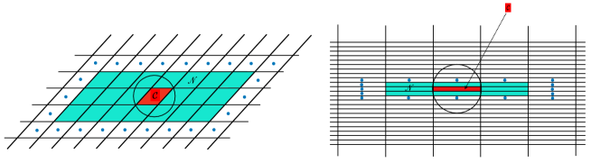
Figure 2: Two fundamental unit cells $\mathcal{C}$ in the doubly periodic case. On the left, the indicated $7\times 3$ grid of neighbors define the near region $\mathcal{N}$ when the parameter $m_{0}=3$. On the right, when $m_{0}=1$, the near region corresponds to the $3\times 3$ grid of neighbors, which is sufficient for rectangular lattices. We also plot the centers of the nearest image cells outside $\mathcal{N}$. Note that if the field due to distant images is represented in the unit cell by a Taylor series, the convergence behavior is controlled by the distance from the smallest disk covering the unit cell $\mathcal{C}$ to the nearest such image, which must lie outside the disk. For the geometry on the left, all image sources outside $\mathcal{N}$ satisfy this constraint and the Taylor series converges. For high aspect ratio cells, illustrated on the right, several of the images lie within the disk, and a region much larger than $\mathcal{N}$ must be excluded for the corresponding Taylor series to be convergent.

Recently, two new approaches were developed that carry out a free space calculation of the form (4) over sources in $\Lambda_{near}$ and correct for the lack of periodicity using an integral representation [2, 3] or a representation in terms of discrete auxiliary Green’s functions [6, 31, 44]. Both of these approaches are effective even for high aspect ratio unit cells, but require the solution of a possibly ill-conditioned linear system of equations in the correction step.

In this paper, we develop a new scheme to treat periodic boundary conditions based on an explicit, low-rank representation for the influence of all distant sources in the far field (those in image cells indexed by $\Lambda_{far}$). It avoids the lattice sum/Taylor series formalism altogether and is insensitive to the aspect ratio of the unit cell. It was motivated by, and makes use of, the fast algorithms for lattice sums and elliptic functions developed in [13, 17, 27, 34] and the fast translation operators used in modern versions of the FMM [11, 24, 26].

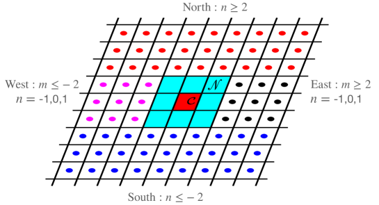
Figure 3: The tiling of the plane in the far region (for doubly periodic problems with $m_{0}=1$) can be decomposed into four parts. The fundamental unit cell is indicated by ${\cal C}$ and the near field by ${\cal N}$. All other copies of the unit cell lie to the “south” (blue, with $n\leq-2$), the “north” (red, with $n\geq 2$), the “west” (magenta, with $n=-1,0,1$ and $m<-1$) or the “east” (black, with $n=-1,0,1$ and $m>1$).

The essence of the approach is easily illustrated in the doubly periodic setting (Figure 3), where the tiling of the far field is divided into four subregions.

Remark 2.

To fix notation, we will denote by ${\bf t}=(x,y)$ or ${\bf t}_{l}=(x_{l},y_{l})$ the coordinates of a target point where we seek to evaluate the field. We will denote by ${\bf s}=(x^{\prime},y^{\prime})$ or ${\bf s}_{j}=(x^{\prime}_{j},y^{\prime}_{j})$ the coordinates of a source point.

Claim 1.

Consider the field induced by all sources lying in image cells with centers lying to the “south”: $\{(m,n)\in\mathbb{Z}^{2}|m\in\mathbb{Z},\ n\leq-2\}$ (Figure 3). Then, for any target ${\bf t}\in\mathcal{C}$,

$$u({\bf t}) =\sum_{j=1}^{N_{S}}\left(\sum_{m=-\infty}^{\infty}\sum_{n=-\infty}^{-2}G({\bf t},{\bf s}_{j}+{\bf l}_{m,n})\right)q_{j}$$ (9)

$$=\sum_{m=-\infty}^{\infty}c_{m}\ e^{-\sqrt{(2\pi m/d)^{2}+\beta^{2}}y}e^{2\pi imx/d}\,,$$

where

$$c_{m}=\frac{\pi}{d}\left(\frac{e^{-2\sqrt{(2\pi m/d)^{2}+\beta^{2}}\eta}e^{-4\pi im\xi/d}}{1-e^{-\sqrt{(2\pi m/d)^{2}+\beta^{2}}\eta}e^{-2\pi im\xi/d}}\right)\,\sum_{j=1}^{N_{S}}q_{j}\frac{e^{\sqrt{(2\pi m/d)^{2}+\beta^{2}}y^{\prime}_{j}}\,e^{-2\pi imx^{\prime}_{j}/d}}{\sqrt{(2\pi m/d)^{2}+\beta^{2}}}\,.$$

We postpone the derivation of this formula to Section 3, but let us briefly examine its consequences. First, the behavior of the series is not controlled by a radius of convergence, as it is for methods based on lattice sums and Taylor series. Second, the series converges exponentially fast. Since $|y|,|y_{j}|\leq\frac{\eta}{2}$, it is easy to see that the $m$th term of the series decays faster than $e^{-2\pi m\eta/d}$. Clearly, approximately $6A$ terms yields double precision accuracy, where $A=d/\eta$ is the aspect ratio of the unit cell. Computing the moments $c_{m}$ requires $O(N_{S}\,A)$ work. Subsequent evaluation at $N_{T}$ target points again requires $O(N_{T}\,A)$ work. In short, this is an efficient low-rank, separable representation of the potential due to a subset of the image sources, the rank of which grows at most linearly with $A$. When $A$ is sufficiently large, we will show how to use the non-uniform FFT (NUFFT) [4, 14, 15, 22, 29] to obtain an algorithm whose cost is of the order $O(\log(1/\epsilon)(A\log A+(N_{S}+N_{T})\log(1/\epsilon)))$.

Below, we complete and generalize the representation (9), permitting the imposition of periodic boundary conditions in one or two directions for a variety of non-oscillatory PDEs in the plane. We will denote by

$$K_{2}^{far}({\bf t},{\bf s})=\sum_{(m,n)\in\Lambda_{far}}G({\bf t},{\bf s}+{\bf l}_{mn})$$ (10)

the far-field kernel for doubly periodic problems. In the singly periodic case, we denote the corresponding far-field kernel by

$$K_{1}^{far}({\bf t},{\bf s})=\sum_{(m,0)\in\Lambda_{far}^{(1)}}G({\bf t},{\bf s}+{\bf l}_{m0})\;.$$ (11)

Definition 3.

Let ${\bf S}=\{{\bf s}_{j}\,|\,j=1,\dots,N_{S}\}$ and ${\bf T}=\{{\bf t}_{l}\,|\,l=1,\dots,N_{T}\}$ denote collections of sources and targets, respectively, in the unit cell $\mathcal{C}$ and let ${\bf q}=(q_{1},\dots,q_{N_{S}})$ denote a vector of “charge” strengths. With a slight abuse of notation, we define the $N_{T}\times N_{S}$ periodizing operators ${\bf P}_{1}={\bf P}_{1}^{\mathcal{C}}({\bf T},{\bf S})$ and ${\bf P}_{2}={\bf P}_{2}^{\mathcal{C}}({\bf T},{\bf S})$ by

$${\bf P}_{1}(l,j)=K_{1}^{far}({\bf t}_{l},{\bf s}_{j})$$

and

$${\bf P}_{2}(l,j)=K_{2}^{far}({\bf t}_{l},{\bf s}_{j}),$$

where the far field kernels $K_{1}^{far}$ and $K_{2}^{far}$ are given by (10) and (11). The vectors

$${\bf P}_{1}{\bf q},\quad{\bf P}_{2}{\bf q}$$

will be referred to as the periodizing potentials. We will omit the superscript and depedence on source and target locations when it is clear from context. We also assume that the governing PDE is clear from context.

It is worth noting that our method yields an explicit, low-rank representation of the periodic Green’s function, without the need to solve any auxillary linear systems. In fact, the periodizing operators ${\bf P}_{2},{\bf P}_{1}$ admit plane-wave factorizations of rank $O(A)$ similar to the formula for the “south” images described above, leading to simple fast algorithms for their evaluation. More precisely, letting $r=O(A)$ be the numerical rank of ${\bf P}_{2}$ or ${\bf P}_{1}$ to precision $\varepsilon$, a simple, direct method requires $O(r(N_{S}+N_{T}))$ work. When $r$ is large, a more elaborate algorithm using the NUFFT requires only $O(\log(1/\epsilon)(r\log r+(N_{S}+N_{T})\log(1/\epsilon)))$ work.

In Section 2, we review the mathematical and computational foundations of the method. In Section 3, we discuss the modified Helmholtz case in detail. In Section 4, we discuss the Poisson equation, where charge neutrality is a necessary constraint. The Stokes and modified Stokes problems are considered in Section 5. In Section 6, we describe the full scheme including NUFFT acceleration. We illustrate the performance of the method in Section 7 with several numerical examples and describe future extensions of the method in Section 8. An extension of our representation for multipole sources is provided in B and C.

2 Mathematical preliminaries

In this section, we summarize the main mathematical tools used in deriving our low-rank representation. These include the Poisson summation formula, Sommerfeld integral representations for free-space Green’s functions, the nonuniform FFT, and high order accurate quadrature schemes.

2.1 The Poisson summation formula

Let $f(x):\mathbb{R}\rightarrow\mathbb{C}$ be a function defined on the real line which has a well-defined Fourier transform

$$\hat{f}(k)=\int_{\mathbb{R}}e^{-ikx}f(x)dx,$$ (12)

for which the Fourier inversion theorem holds. That is,

$$f(x)=\frac{1}{2\pi}\int_{\mathbb{R}}e^{ikx}\hat{f}(k)dk.$$

The Poisson summation formula (see, for example, [16]) then states that

$$\sum_{n=-\infty}^{\infty}f\left(x+\frac{2\pi n}{h}\right)=\frac{h}{2\pi}\sum_{m=-\infty}^{\infty}\hat{f}(mh)e^{imhx}.$$ (13)

This holds for a broad class of functions, and extends to distributions such as the Dirac delta function. In the latter case, we have [28]

$$\sum_{n=-\infty}^{\infty}\delta\left(x+\frac{2\pi n}{h}\right)=\frac{h}{2\pi}\sum_{m=-\infty}^{\infty}e^{imhx}.$$ (14)

2.2 Plane wave representations for the modified Helmholtz equation

The Green’s function for the modified Bessel function, $K_{0}(\beta\sqrt{x^{2}+y^{2}})$, and its higher order multipole terms have the well-known Sommerfeld integral representation [36, 34, 38]:

$$K_{l}\left(\beta\sqrt{x^{2}+y^{2}}\right)e^{il\phi}=\left\{\begin{aligned} &\frac{i^{l}}{2\beta^{l}}\int_{-\infty}^{\infty}\left(\sqrt{\lambda^{2}+\beta^{2}}-\lambda\right)^{l}\frac{e^{-\sqrt{\lambda^{2}+\beta^{2}}y}}{\sqrt{\lambda^{2}+\beta^{2}}}e^{i\lambda x}d\lambda,\quad y>0,\\ &\frac{(-i)^{l}}{2\beta^{l}}\int_{-\infty}^{\infty}\left(\sqrt{\lambda^{2}+\beta^{2}}+\lambda\right)^{l}\frac{e^{\sqrt{\lambda^{2}+\beta^{2}}y}}{\sqrt{\lambda^{2}+\beta^{2}}}e^{i\lambda x}d\lambda,\quad y<0,\\ &\frac{1}{2\beta^{l}}\int_{-\infty}^{\infty}\left(\sqrt{\lambda^{2}+\beta^{2}}+\lambda\right)^{l}\frac{e^{-\sqrt{\lambda^{2}+\beta^{2}}x}}{\sqrt{\lambda^{2}+\beta^{2}}}e^{i\lambda y}d\lambda,\quad x>0,\\ &\frac{(-1)^{l}}{2\beta^{l}}\int_{-\infty}^{\infty}\left(\sqrt{\lambda^{2}+\beta^{2}}-\lambda\right)^{l}\frac{e^{\sqrt{\lambda^{2}+\beta^{2}}x}}{\sqrt{\lambda^{2}+\beta^{2}}}e^{i\lambda y}d\lambda,\quad x<0,\end{aligned}\right.$$ (15)

for $l\geq 0$.

2.2.1 Plane wave representations for the Poisson equation

The plane-wave expansion of the Green’s function for the Laplacian is typically invoked for the complex analytic function

$$\frac{1}{z}=\frac{1}{x+iy}=\frac{x-iy}{x^{2}+y^{2}}=-\left(\frac{\partial}{\partial x}-i\,\frac{\partial}{\partial y}\right)\log(1/\sqrt{x^{2}+y^{2}})\,,$$

rather than $\log(1/\sqrt{x^{2}+y^{2}})$ itself. This is sufficient for our purposes, where we assume the collection of sources in the unit cell $\mathcal{C}$ satisfies charge neutrality:

$$\sum_{j=1}^{N_{S}}q_{j}=0.$$ (16)

In C, we will consider multipole sources as well as charge distributions, and will make use of the representations:

$$\frac{1}{z^{l}}=\left\{\begin{aligned} &\frac{1}{(l-1)!}\,\int_{0}^{\infty}\lambda^{l-1}e^{-\lambda z}d\lambda,\quad x>0,\\ &\frac{(-1)^{l}}{(l-1)!}\,\int_{0}^{\infty}\lambda^{l-1}e^{\lambda z}d\lambda,\quad x<0,\\ &\frac{(-i)^{l}}{(l-1)!}\,\int_{0}^{\infty}\lambda^{l-1}e^{i\lambda z}d\lambda,\quad y>0,\\ &\frac{i^{l}}{(l-1)!}\,\int_{0}^{\infty}\lambda^{l-1}e^{-i\lambda z}d\lambda,\quad y<0,\end{aligned}\right.$$ (17)

for $l\geq 1$. These representations are useful in developing diagonal translation operators for FMMs [11, 26] as well as for the computation of harmonic lattice sums and elliptic functions [27]. Note that the integrals in Eq. 17 are consistent with (15). In the case $l=1$, for example, this requires taking the limit $\beta\rightarrow 0$ and using the formula [38, §10.30.2]:

$$\lim_{\beta\rightarrow 0}\beta K_{1}(\beta r)e^{-i\theta}=\frac{1}{z},\quad z=re^{i\theta}.$$ (18)

2.2.2 Generalized Gaussian quadrature for the doubly periodic case

In evaluating the integrals in (15) or (17), we will require suitable quadrature rules. More generally, we would like efficient rules of the form

$$\int_{0}^{\infty}\frac{e^{-\sqrt{\lambda^{2}+\beta^{2}}x}}{\sqrt{\lambda^{2}+\beta^{2}}}[M_{1}(\lambda)e^{i\lambda y}+{M_{1}(-\lambda)}e^{-i\lambda y}]\,d\lambda$$

$$\approx\sum_{k=1}^{N}\frac{e^{-\sqrt{\lambda_{k}^{2}+\beta^{2}}x}}{\sqrt{\lambda_{k}^{2}+\beta^{2}}}[M_{1}(\lambda_{k})e^{i\lambda_{k}y}+M_{1}(-\lambda_{k})e^{-i\lambda_{k}y}]\,w_{k}$$

and

$$\int_{0}^{\infty}e^{-\lambda z}M(\lambda)d\lambda\approx\sum_{k=1}^{N}e^{-\lambda_{k}z}M(\lambda_{k})w_{k}$$

for $(x,y)$ in a bounded domain of $\mathbb{R}^{2}$. The functions $M_{1}(\lambda)$ and $M(\lambda)$ here are smooth functions of $\lambda$ that depend on the source locations and strengths and are derived from the infinite series that appear in the periodizing operators. The remaining cases in (15) or (17) are treated using the same nodes and weights. Because we have separated the near and far fields, we will be using these rules under restrictive conditions on $x,y$. As we shall see below in more detail, for the doubly periodic case we will typically invoke the quadrature under suitable rescaling so that $x\in[1,7]$ and $y\in[-2,2]$. Finding optimal weights and nodes for this restricted range of arguments leads to a nonlinear optimization problem which can be solved by what is known as generalized Gaussian quadrature [9, 32, 46].

For the modified Hemholtz equation, if $\beta$ is bounded away from zero, the integral converges and the number of nodes depends rather weakly on $\beta$ itself. We note, however, that in the limit $\beta=0$, the modified Helmholtz integral (for $x>0$) becomes

$$\int_{0}^{\infty}\frac{e^{-\lambda x}}{\lambda}[M_{1}(\lambda)e^{i\lambda y}+{M_{1}(-\lambda)}e^{-i\lambda y}]d\lambda,\quad x>0,$$

with $M_{1}(\lambda)=O(1/\lambda)$. Thus, significant adjustments would be required as $\beta\rightarrow 0$ to handle the near hypersingularity at the origin. In the present context, where we seek to impose periodicity, charge neutrality is a natural condition (see Section 4).

For the modified Helmholtz equation, special purpose quadratures have been constructed for $\beta$ in different ranges. The number of quadrature nodes decreases as $\beta$ increases. For $\beta\in[10^{-6},+\infty)$, $x\in[1,7]$, $y\in[-2,2]$, at most 21 nodes have been found to yield six digits of accuracy and at most 41 nodes have been found to yield twelve digits of accuracy. When $\beta>22$, only 1 node is sufficient for six digits of accuracy. When $\beta>37$, 3 nodes are sufficient for twelve digits of accuracy. For the Poisson equation, with $x\in[1,7]$, $y\in[-2,2]$, 18 nodes yield six digits of accuracy and 29 nodes yield twelve digits of accuracy. We omit consideration of the modified Helmholtz equation when $\beta<10^{-6}$ but charge neutrality is not satisfied, as this is a highly ill-conditioned problem. Assuming charge neutrality, one may simply use the quadrauture designed for the Poisson equation.

2.3 The non-uniform fast Fourier transform

For high aspect ratio unit cells, we will require the evaluation of discrete Fourier transforms where the nodes, frequencies, or both are not uniformly spaced. By combining the standard fast Fourier transform (FFT) with careful analysis and fast interpolation techniques, these sums can be computed with nearly optimal computational complexity. The resulting algorithms are known as non-uniform fast Fourier transforms (NUFFTs). They were originally described in [14, 15]. We refer the reader to [4, 5] for recent references and a state-of-the-art implementation.

The type-I NUFFT evaluates sums of the form

$$f_{k}=\sum_{j=1}^{N}c_{j}e^{ikx_{j}}\;,\textrm{ for }k=-M,\ldots,M.$$ (19)

Letting ${\bf f}=(f_{-M},\dots,f_{M-1},f_{M})$ and letting ${\bf c}=(c_{1},\dots,c_{N})$, we will write

$${\bf f}={\bf N}{\bf c}.$$

When the explicit dependence on the point locations $\{x_{j}\}$ and the number of Fourier modes $M$ are needed, we will denote the operator ${\bf N}$ by ${\bf N}(\{x_{j}\};M)$. The operator ${\bf N}$ can be applied using $O(M\log M+N\log(1/\epsilon))$ operations with nearly the same performance as the standard FFT.

Given the vector ${\bf f}$, The type-II NUFFT evaluates sums of the form

$$v_{j}=\sum_{k=-M}^{M}f_{k}e^{-ix_{j}k}\;,\textrm{ for }j=1,\ldots,N\;,$$ (20)

corresponding to the adjoint of ${\bf N}$:

$${\bf v}={\bf N}^{\ast}{\bf f},$$

with the same computational complexity, where ${\bf v}=(v_{1},\dots,v_{N})$.

2.4 Legendre polynomials and barycentric interpolation

The standard Legendre polynomials can be defined by setting $P_{0}\equiv 1$ and $P_{1}(t)=t$, with higher degree polynomials defined by the recurrence formula

$$(l+1)P_{l+1}(t)=(2l+1)tP_{l}(t)-lP_{l-1}(t)\;.$$

Let $-1<t_{1}<\cdots<t_{M}<1$ be the roots of $P_{M}$, known as the Legendre nodes of order $M$.

Letting $f$ be a function defined on $[-1,1]$, the degree $M-1$ polynomial, $p_{M}[f]$, which interpolates $f$ at the Legendre nodes of order $M$, can be written in the form

$$p_{M}[f](t)=\frac{\sum_{i=1}^{M}\frac{\sigma_{i}}{t-t_{i}}f(t_{i})}{\sum_{i=1}^{M}\frac{\sigma_{i}}{t-t_{i}}}\;,$$ (21)

where

$$\sigma_{i}=\frac{1}{\prod_{j\neq i}\left(t_{i}-t_{j}\right)}\;.$$ (22)

This is known as the second form of the barycentric formula for the interpolant.

As observed in [43], if $f$ is analytic in the Bernstein ellipse with foci at $\pm 1$ and semi-major and semi-minor lengths adding up to $\rho>1$, then

$$\|f-p_{M}[f]\|_{\infty}\leq(1+\Lambda_{M})\frac{2C}{\rho^{M}(\rho-1)}\;,$$ (23)

where $\|\cdot\|_{\infty}$ is the maximum norm on $[-1,1]$, $C$ is a constant so that $|f|\leq C$ on the Bernstein ellipse, and $\Lambda_{M}=O(\sqrt{M})$ is the Lebesgue constant for the nodes. Thus, the interpolant is a spectrally accurate approximation of $f$. See [19, 25, 42, 43] for further details.

3 Periodicity for the modified Helmholtz equation

In this section, we consider the imposition of periodic boundary conditions for the two-dimensional modified Helmholtz equation with either one or two directions of periodicity. This requires an efficient scheme for the evaluation of the field due to all image sources in the far field (outside the nearest neighbors of $\mathcal{C}$). For simplicity, we fix $m_{0}=1$ when considering periodicity in the the ${\hat{\bf e}}_{1}=(d,0)$ direction alone and $m_{0}=3$ when considering periodicty in both the ${\hat{\bf e}}_{1}=(d,0)$ and ${\hat{\bf e}}_{2}=(\xi,\eta)$ directions. Since the governing Green’s function is exponentially decaying, all of the infinite series in the definition of the periodizing operators in (3) converge absolutely.

Our algorithm is based on splitting the far field kernels into two parts for singly periodic case,

$$K_{1}^{west}({\bf t},{\bf s}) =\sum_{m=-\infty}^{-2}G({\bf t},{\bf s}+(md,0)),$$ (24)

$$K_{1}^{east}({\bf t},{\bf s}) =\sum_{m=2}^{\infty}G({\bf t},{\bf s}+(md,0)),$$

and four parts (as in Figure 3) for the doubly periodic case:

$$K_{2}^{west}({\bf t},{\bf s}) =\sum_{n=-1}^{1}\sum_{m=-\infty}^{-4}G({\bf t},{\bf s}+{\bf l}_{mn}),$$ (25)

$$K_{2}^{east}({\bf t},{\bf s}) =\sum_{n=-1}^{1}\sum_{m=4}^{\infty}G({\bf t},{\bf s}+{\bf l}_{mn}),$$

$$K_{2}^{south}({\bf t},{\bf s}) =\sum_{n=-\infty}^{-2}\sum_{m=-\infty}^{\infty}G({\bf t},{\bf s}+{\bf l}_{mn}),$$

$$K_{2}^{north}({\bf t},{\bf s}) =\sum_{n=2}^{\infty}\sum_{m=-\infty}^{\infty}G({\bf t},{\bf s}+{\bf l}_{mn}).$$

The corresponding operators will be denoted by ${\bf P}_{1}^{west}$, ${\bf P}_{1}^{east}$, ${\bf P}_{2}^{west}$, ${\bf P}_{2}^{east}$, ${\bf P}_{2}^{south}$ and ${\bf P}_{2}^{north}$, so that

$${\bf P}_{1} ={\bf P}_{1}^{west}+{\bf P}_{1}^{east},$$ (26)

$${\bf P}_{2} ={\bf P}_{2}^{west}+{\bf P}_{2}^{east}+{\bf P}_{2}^{south}+{\bf P}_{2}^{north}.$$

Theorem 1.

Let ${\bf S}=\{{\bf s}_{j}\,|\,j=1,\dots,N_{S}\}$ and ${\bf T}=\{{\bf t}_{l}\,|\,l=1,\dots,N_{T}\}$ denote collections of sources and targets in the unit cell $\mathcal{C}$ and let ${\bf P}_{2}^{south}$ denote the $N_{T}\times N_{S}$ operator with ${\bf P}_{2}^{south}(l,j)=K_{2}^{south}({\bf t}_{l},{\bf s}_{j})$. Given a precision $\epsilon$, let

$$M=\left\lceil\frac{d}{2\pi\eta}\log\left(\frac{1}{1-e^{-\frac{2\pi\eta}{d}}}\frac{1}{\epsilon}\right)\right\rceil\approx\frac{A}{2\pi}(\log(A)+\log(1/\epsilon)).$$ (27)

For $m=-M,\dots,M$, let

$$\alpha_{m}=\frac{2\pi m}{d},\quad\chi_{m}=\sqrt{\alpha_{m}^{2}+\beta^{2}},\quad Q_{m}=\chi_{m}\eta-i\alpha_{m}\xi\,.$$ (28)

Let ${\bf L}^{south}\in\mathbb{C}^{N_{T}\times(2M+1)}$ and ${\bf R}^{south}\in\mathbb{C}^{(2M+1)\times N_{S}}$ be dense matrices and let ${\bf D}^{south}\in\mathbb{C}^{(2M+1)\times(2M+1)}$ be a diagonal matrix with

$${\bf L}^{south}(l,m) =e^{-\chi_{m}y_{l}}e^{i\alpha_{m}x_{l}}\,,$$ (29)

$${\bf R}^{south}(m,j) =e^{\chi_{m}y^{\prime}_{j}}\,e^{-i\alpha_{m}x^{\prime}_{j}}\,,$$

$${\bf D}^{south}(m,m) =\frac{1}{2d\,\chi_{m}}\frac{e^{-2Q_{m}}}{1-e^{-Q_{m}}}.$$

Then

$${\bf P}_{2}^{south}={\bf L}^{south}\,{\bf D}^{south}\,{\bf R}^{south}+O(\epsilon).$$ (30)

Proof.

Combining (15) and (25), we obtain

$$K_{2}^{south}({\bf t},{\bf s}_{j}) =\sum_{n=-\infty}^{-2}\sum_{m=-\infty}^{\infty}\int_{-\infty}^{\infty}\frac{e^{-\sqrt{\lambda^{2}+\beta^{2}}(y-y^{\prime}_{j}-n\eta)}}{4\pi\sqrt{\lambda^{2}+\beta^{2}}}\,e^{i\lambda(x-x^{\prime}_{j}-md-n\xi)}d\lambda$$ (31)

$$=\sum_{n=-\infty}^{-2}\sum_{m=-\infty}^{\infty}\int_{-\infty}^{\infty}\frac{e^{-\sqrt{\lambda^{2}+\beta^{2}}(y-y^{\prime}_{j}-n\eta)}}{\sqrt{\lambda^{2}+\beta^{2}}}\,e^{i\lambda(x-x^{\prime}_{j}-n\xi)}\frac{1}{2d}\delta\left(\lambda-\frac{2\pi m}{d}\right)d\lambda$$

$$=\sum_{n=-\infty}^{-2}\sum_{m=-\infty}^{\infty}\frac{1}{2d}\frac{e^{-\chi_{m}(y-y^{\prime}_{j}-n\eta)}}{\chi_{m}}\,e^{i\alpha_{m}(x-x^{\prime}_{j}-n\xi)},$$

where $\chi_{m},\alpha_{m}$ are given by Eq. 28. The last two equalities follow from the Poisson summation formula Eq. 14 and the Dirac delta function property. Exchanging the order of summation and summing the relevant geometric series in $n$ leads to

$$K_{2}^{south}({\bf t},{\bf s}_{j})=\frac{1}{2d}\sum_{m=-\infty}^{\infty}\frac{e^{-\chi_{m}(y-y^{\prime}_{j})+i\alpha_{m}(x-x^{\prime}_{j})}}{\chi_{m}}\frac{e^{-2Q_{m}}}{1-e^{-Q_{m}}}$$ (32)

where $Q_{m}$ is given in Eq. 28.

Truncating the sum at $|m|=M$ yields the $(2M+1)$ term approximation

$${K_{2,M}}^{south}({\bf t},{\bf s}_{j})=\frac{1}{2d}\sum_{m=-M}^{M}\frac{e^{-\chi_{m}(y-y^{\prime}_{j})+i\alpha_{m}(x-x^{\prime}_{j})}}{\chi_{m}}\frac{e^{-2Q_{m}}}{1-e^{-Q_{m}}}$$ (33)

and the formulas in Eq. 29.

We now estimate the truncation error

$$E_{s}=|{K_{2}}^{south}({\bf t},{\bf s}_{j})-{K_{2.M}}^{south}({\bf t},{\bf s}_{j})|.$$ (34)

For any $m\in\mathbb{Z}$, it is easy to verify that

$$\chi_{m}\geq\frac{2\pi|m|}{d},\ \left|e^{-\chi_{m}(y-y_{j})-Q_{m}}\right|=\left|e^{-\chi_{m}(\eta+y-y_{j})}\right|\leq 1,$$

$$\left|e^{-Q_{m}}\right|\leq e^{-\chi_{m}\eta},\ \left|1-e^{-Q_{m}}\right|\geq 1-e^{-\chi_{m}\eta}.$$

From these bounds, it follows that

$$E_{s} \leq\frac{1}{d}\sum_{m=M+1}^{\infty}\frac{1}{\chi_{m}}\frac{e^{-\chi_{m}\eta}}{1-e^{-\chi_{m}\eta}}<\frac{1}{M+1}\frac{e^{-\frac{2\pi(M+1)\eta}{d}}}{1-e^{-\frac{2\pi(M+1)\eta}{d}}}\sum_{k=0}^{\infty}e^{-\frac{2\pi k\eta}{d}}$$ (35)

$$=\frac{1}{2\pi(M+1)}\frac{e^{-\frac{2\pi(M+1)\eta}{d}}}{\left(1-e^{-\frac{2\pi(M+1)\eta}{d}}\right)\left(1-e^{-\frac{2\pi\eta}{d}}\right)}.$$

with $M$ given by Eq. 27. The estimate Eq. 30 follows, completing the proof. $\Box$

Remark 3.

Theorem 1 yields a truncated version of the formula Eq. 9 with weights ${\bf c}=(c_{-M},c_{-M+1},\dots,c_{M-1},c_{M})$ given by

$${\bf c}={\bf D}^{south}\,{\bf R}^{south}{\bf q}\,,$$

where ${\bf q}=(q_{1},\dots,q_{N_{S}})$ is the vector of charge strengths.

Remark 4.

When $\beta\gg 1$, the value of $M$ in Eq. 27 can be shown to be even smaller, but since the cost is logarithmic in $A$ and $\epsilon$ we omit this more detailed analysis.

Remark 5.

The observation that Poisson summation yields rapidly converging series approximations for lines or half spaces of lattice points that do not pass through the origin was made in [17, 34] for the purpose of computing lattice sums.

Essentially the same analysis yields

Corollary 1.

The matrix ${\bf P}_{2}^{north}$ has the low-rank factorization

$${\bf P}_{2}^{north}={\bf L}^{north}\,{\bf D}^{north}\,{\bf R}^{north}+O(\epsilon)$$

where ${\bf D}^{north}=\overline{{\bf D}^{south}}$,

$${\bf L}^{north}(l,m) =e^{\chi_{m}y_{l}}e^{i\alpha_{m}x_{l}}\,,$$ (36)

$${\bf R}^{north}(m,j) =e^{-\chi_{m}y^{\prime}_{j}}\,e^{-i\alpha_{m}x^{\prime}_{j}}\,.$$

Definition 4.

Since the rank is precision-dependent, we say that ${\bf P}_{2}^{north}$ has an $\epsilon$-rank of $2M+1$.

It remains to consider the “west” and “east” contributions.

Theorem 2.

Let ${\bf t},{\bf s}_{j}$ lie in a unit cell $\mathcal{C}$ and $m_{0}=1$. Then, the kernels $K_{1}^{west}$ and $K_{1}^{east}$ have the integral representations

$$K_{1}^{west}({\bf t},{\bf s}_{j}) =\int_{-\infty}^{\infty}\frac{e^{-\sqrt{\lambda^{2}+\beta^{2}}(x-x^{\prime}_{j})}}{4\pi\sqrt{\lambda^{2}+\beta^{2}}}\,e^{i\lambda(y-y^{\prime}_{j})}\frac{e^{-2\sqrt{\lambda^{2}+\beta^{2}}d}}{1-e^{-\sqrt{\lambda^{2}+\beta^{2}}d}}d\lambda,$$ (37)

$$K_{1}^{east}({\bf t},{\bf s}_{j}) =\int_{-\infty}^{\infty}\frac{e^{\sqrt{\lambda^{2}+\beta^{2}}(x-x^{\prime}_{j})}}{4\pi\sqrt{\lambda^{2}+\beta^{2}}}\,e^{i\lambda(y-y^{\prime}_{j})}\frac{e^{-2\sqrt{\lambda^{2}+\beta^{2}}d}}{1-e^{-\sqrt{\lambda^{2}+\beta^{2}}d}}d\lambda.$$

Letting $m_{0}=3$ with the additional assumption with $d\geq\sqrt{\xi^{2}+\eta^{2}}$, the kernels $K_{2}^{west}$ and $K_{2}^{east}$ have the integral representations

$$K_{2}^{west}({\bf t},{\bf s}_{j}) =\sum_{n=-1}^{1}\int_{-\infty}^{\infty}\frac{e^{-\sqrt{\lambda^{2}+\beta^{2}}(x-x^{\prime}_{j}-n\xi)}}{4\pi\sqrt{\lambda^{2}+\beta^{2}}}\,e^{i\lambda(y-y^{\prime}_{j}-n\eta)}\frac{e^{-4\sqrt{\lambda^{2}+\beta^{2}}d}}{1-e^{-\sqrt{\lambda^{2}+\beta^{2}}d}}d\lambda,$$ (38)

$$K_{2}^{east}({\bf t},{\bf s}_{j}) =\sum_{n=-1}^{1}\int_{-\infty}^{\infty}\frac{e^{\sqrt{\lambda^{2}+\beta^{2}}(x-x^{\prime}_{j}-n\xi)}}{4\pi\sqrt{\lambda^{2}+\beta^{2}}}\,e^{i\lambda(y-y^{\prime}_{j}-n\eta)}\frac{e^{-4\sqrt{\lambda^{2}+\beta^{2}}d}}{1-e^{-\sqrt{\lambda^{2}+\beta^{2}}d}}d\lambda.$$

Proof.

These formulas follow directly from Eq. 15 and Eq. 24 and summation of the geometric series in $m$. In the singly periodic case, excluding one nearest neighbor from either side is sufficient to ensure the exponential decay of the integrand in (37). In the doubly periodic case, with a parallelogram as the unit cell, we must ensure that we are using the integral representation of the modified Bessel function where it is valid and that the resulting integrand decays exponentially fast. For this, we must have that $x-x^{\prime}-md-n\xi>d$ for all $m\leq-(m_{0}+1)$ and $|n|\leq 1$ in the “west” case, and $x-x^{\prime}+md-n\xi>d$ for all $m\geq m_{0}+1$ and $|n|\leq 1$ in the “east” case. It is straightforward to verify that if $m_{0}=3$, then $x-x^{\prime}-md-n\xi\geq 4d-(d+\xi)-\xi>d$ in the first instance and that $x-x^{\prime}+md-n\xi>d$ in the second instance under the stated assumption about the unit cell. $\Box$

The reader will note that there is a major difference between the east/west representations and those for the north and south. The latter are fully discrete, while for the east and west representations, we have an integral that needs to be evaluated before we can develop a low-rank decomposition. For this, we will make use of numerical quadrature, in order to develop a low-rank approximation of precision $\epsilon$. This provides a discrete approximation of the Sommerfeld representation for $K_{1}^{west}({\bf t},{\bf s}_{j})$ and $K_{2}^{west}({\bf t},{\bf s}_{j})$ in Eqs. 37 and 38 rewritten in the form

$$K_{1}^{west}({\bf t},{\bf s}_{j}) =\Re\left(\int_{0}^{\infty}\frac{e^{-\sqrt{\lambda^{2}+\beta^{2}}(x-x^{\prime}_{j})}}{2\pi\sqrt{\lambda^{2}+\beta^{2}}}\,e^{i\lambda(y-y^{\prime}_{j})}\frac{e^{-2\sqrt{\lambda^{2}+\beta^{2}}d}}{1-e^{-\sqrt{\lambda^{2}+\beta^{2}}d}}d\lambda\right)$$ (39)

$$\approx\Re\Bigg{(}\sum_{n=1}^{N^{1}_{q}(\beta,d,\eta)}w_{n,1}(\beta,d,\eta)\frac{e^{-\sqrt{\lambda_{n,1}^{2}+\beta^{2}}(x-x^{\prime}_{j})}}{2\pi\sqrt{\lambda_{n,1}^{2}+\beta^{2}}}\,e^{i\lambda_{n,1}(y-y^{\prime}_{j})}\frac{e^{-2\sqrt{\lambda_{n,1}^{2}+\beta^{2}}d}}{1-e^{-\sqrt{\lambda_{n,1}^{2}+\beta^{2}}d}}\Bigg{)}.$$

$$K_{2}^{west}({\bf t},{\bf s}_{j}) =\Re\Bigg{(}\int_{0}^{\infty}\frac{e^{-\sqrt{\lambda^{2}+\beta^{2}}(x-x^{\prime}_{j})}}{2\pi\sqrt{\lambda^{2}+\beta^{2}}}\,e^{i\lambda(y-y^{\prime}_{j})}\frac{e^{-4\sqrt{\lambda^{2}+\beta^{2}}d}}{1-e^{-\sqrt{\lambda^{2}+\beta^{2}}d}}$$

$$\hskip 72.26999pt[e^{-\sqrt{\lambda^{2}+\beta^{2}}\xi+i\lambda\eta}+e^{\sqrt{\lambda^{2}+\beta^{2}}\xi-i\lambda\eta}+1]\,d\lambda\Bigg{)}$$

$$\approx\Re\Bigg{(}\sum_{n=1}^{N^{2}_{q}(\beta,d,\eta)}w_{n,2}(\beta,d,\eta)\frac{e^{-\sqrt{\lambda_{n,2}^{2}+\beta^{2}}(x-x^{\prime}_{j})}}{2\pi\sqrt{\lambda_{n,2}^{2}+\beta^{2}}}\,e^{i\lambda_{n,2}(y-y^{\prime}_{j})}\frac{e^{-4\sqrt{\lambda_{n,2}^{2}+\beta^{2}}d}}{1-e^{-\sqrt{\lambda_{n,2}^{2}+\beta^{2}}d}}$$

$$\hskip 72.26999pt[e^{-\sqrt{\lambda_{n,2}^{2}+\beta^{2}}\xi+i\lambda_{n,2}\eta}+e^{\sqrt{\lambda_{n,2}^{2}+\beta^{2}}\xi-i\lambda_{n,2}\eta}+1]\,\Bigg{)}.$$

Note that different numbers of nodes may be needed for the two cases. We denote by $N^{1}_{q}$ and $N^{2}_{q}$ the number of nodes needed for $K_{1}^{west}$ and $K_{2}^{west}$, respectively, with weights and nodes $\{w_{n,1},\lambda_{n,1}\}$ and $\{w_{n,2},\lambda_{n,2}\}$.

In both cases, we define $\lambda^{\prime}=\lambda/d$ so that the decaying exponential in the integrand decays at least as fast as $e^{-\sqrt{\lambda^{\prime 2}+\tilde{\beta}^{2}}}$ ($\tilde{\beta}=\beta\cdot d$). In the doubly periodic case, this leads to the consideration of the integrals in subsection 2.2.2 where $(x,y)\in[1,7]\times[-2,2]$. Generalized Gaussian quadrature can be applied to construct numerical quadratures for a given precision $\epsilon$, with a weak dependence on $\beta$. These quadratures are valid for unit cells with arbitrary geometric parameters and thus can be precomputed and stored [9, 32, 46].

In the singly periodic case, $x$ lies in $[1,3]$, while the range of $y$ can be very large when $\eta\gg d$, leading to highly oscillatory integrals. In this case, the quadrature is constructed as follows. First, the interval $[0,\infty)$ is truncated to $[0,L]$, which can be accomplished easily due to the exponential decay in the $x$ variable, with $L=\sqrt{(\log(1/\epsilon))^{2}-\beta^{2}}$. If $\log(1/\epsilon)\leq\beta$, we can set $L=0$, since the whole integral is then negligible. Second, in order to accurately capture the oscillatory behavior in the $y$ variable, the interval $[0,L]$ is further divided into subintervals $[j\lambda_{0},(j+1)\lambda_{0}]$ for $j=0,\ldots,\lceil L/\lambda_{0}\rceil$, where $\lambda_{0}=2\pi d/\eta$. A shifted and scaled $n$ point Gauss-Legendre quadrature rule (with $n=O(\log(1/\epsilon))$) is then applied to discretize the integral on each subinterval $[j\lambda_{0},(j+1)\lambda_{0}]$ for $j\geq 1$. Third, when $\beta$ is very small, a new difficulty emerges - namely that the integrand is nearly singular at the origin. In that case, we further divide $[0,\lambda_{0}]$ into dyadic subintervals $[0,a]$ and $[2^{k-1}a,2^{k}a]$ for $k=1,\ldots,l_{\rm max}$, where $l_{\rm max}=\lceil\log_{2}(\lambda_{0}/\beta)\rceil$ and $a=\lambda_{0}/l_{\rm max}$. A shifted and scaled $n$ point Gauss-Legendre quadrature rule is again applied to discretize the integral on each such subinterval. To summarize, the total number of quadrature nodes $N_{q}^{1}$ (i.e., the numerical rank of the periodizing operator) is $O\left(\log(1/\epsilon)\left(\log(1/\beta)+\log(1/\epsilon)\cdot\lceil\frac{\eta}{d}\rceil\right)\right)$. In the limit $\beta\rightarrow 0$, it is also possible to develop asymptotic expansions in $\beta$, which we do not consider here.

Remark 6.

The difference between the singly and doubly periodic cases seems rather significant in terms of quadrature design. However, this distinction is somewhat artificial. The reason that the quadrature problem is simple in the doubly periodic case is that we have the freedom to choose which lattice vector is oriented along the $x$-axis. The difficult direction to deal with is the short axis of the unit cell and, by our convention, this makes the north/south periodizing kernels more oscillatory which are already discrete. Thus, the number of terms in the plane-wave expansion for the north/south parts will grow linearly with respect to the aspect ratio $\frac{d}{\eta}$ but without the need for quadrature design.

To summarize, the numerical rank of the periodizing operators may grow linearly with respect to the aspect ratio for both singly and doubly periodic problems. When the rank $r$ is large, the NUFFT can be used to reduce the computational cost from $O(r(N_{T}+N_{S}))$ to $O(\log(1/\epsilon)(r\log r+(N_{T}+N_{S})\log(1/\epsilon)))$ with $\epsilon$ the prescribed precision.

Theorem 3.

Let ${\bf S}=\{{\bf s}_{j}\,|\,j=1,\dots,N_{S}\}$ and ${\bf T}=\{{\bf t}_{l}\,|\,l=1,\dots,N_{T}\}$ denote collections of sources and targets in the unit cell $\mathcal{C}$ and let ${\bf P}_{1}^{west},{\bf P}_{2}^{west}$ denote the $N_{T}\times N_{S}$ operators with ${\bf P}_{1}^{west}(l,j)=K_{1}^{west}({\bf t}_{l},{\bf s}_{j})$ and ${\bf P}_{2}^{west}(l,j)=K_{2}^{west}({\bf t}_{l},{\bf s}_{j})$. Given a precision $\epsilon$, let $N^{1}_{q}(\beta,d,\eta),N^{2}_{q}(\beta,d,\eta)$ denote the number of points needed in the numerical quadrature for $K_{1}^{west}({\bf t},{\bf s})$ and $K_{2}^{west}({\bf t},{\bf s})$, with weights and nodes $\{w_{n,1},\lambda_{n,1}\}$ $\{w_{n,2},\lambda_{n,2}\}$, respectively. Let ${\bf L}_{1}^{west}\in\mathbb{C}^{N_{T}\times N^{1}_{q}}$, ${\bf L}_{2}^{west}\in\mathbb{C}^{N_{T}\times N^{2}_{q}}$, ${\bf R}_{1}^{west}\in\mathbb{C}^{N^{1}_{q}\times N_{S}}$, ${\bf R}_{2}^{west}\in\mathbb{C}^{N^{2}_{q}\times N_{S}}$ be dense matrices and let ${\bf D}_{1}^{e/w}$, ${\bf D}_{2}^{west}$ be diagonal matrices of dimension $N^{1}_{q}$ and $N^{2}_{q}$, respectively, with

$${\bf L}_{1}^{west}(l,n) =e^{-\sqrt{\lambda_{n,1}^{2}+\beta^{2}}x_{l}}e^{i\lambda_{n,1}y_{l}}\,,$$ (40)

$${\bf L}_{2}^{west}(l,n) =e^{-\sqrt{\lambda_{n,2}^{2}+\beta^{2}}x_{l}}e^{i\lambda_{n,2}y_{l}}\,,$$

$${\bf R}_{1}^{west}(n,j) =e^{\sqrt{\lambda_{n,1}^{2}+\beta^{2}}x^{\prime}_{j}}\,e^{-i\lambda_{n,1}y^{\prime}_{j}}\,,$$

$${\bf R}_{2}^{west}(n,j) =e^{\sqrt{\lambda_{n,2}^{2}+\beta^{2}}x^{\prime}_{j}}\,e^{-i\lambda_{n,2}y^{\prime}_{j}}\,,$$

$${\bf D}_{1}^{e/w}(n,n) =\frac{1}{2\pi}\frac{w_{n,1}}{\sqrt{\lambda_{n,1}^{2}+\beta^{2}}}\frac{e^{-2\sqrt{\lambda_{n,1}^{2}+\beta^{2}}d}}{1-e^{-\sqrt{\lambda_{n,1}^{2}+\beta^{2}}d}}\,,$$

$${\bf D}_{2}^{west}(n,n) =\frac{w_{n,2}}{\sqrt{\lambda_{n,2}^{2}+\beta^{2}}}\frac{e^{-4\sqrt{\lambda_{n,2}^{2}+\beta^{2}}d}}{1-e^{-\sqrt{\lambda_{n,2}^{2}+\beta^{2}}d}}\frac{[e^{-\sqrt{\lambda_{n,2}^{2}+\beta^{2}}\xi+i\lambda_{n,2}\eta}+e^{\sqrt{\lambda_{n,2}^{2}+\beta^{2}}\xi-i\lambda_{n,2}\eta}+1]}{2\pi}.$$

Let

$${\bf P}_{1}^{west} ={\bf L}_{1}^{west}\,{\bf D}_{1}^{e/w}\,{\bf R}_{1}^{west},$$

$${\bf P}_{2}^{west} ={\bf L}_{2}^{west}\,{\bf D}_{2}^{west}\,{\bf R}_{2}^{west}.$$

Then the real parts of the vectors

$${\bf P}_{1}^{west}{\bf q},\ {\bf P}_{2}^{west}{\bf q}$$

denote the contributions from the west sources to the corresponding periodizing potentials.

Corollary 2.

The matrices ${\bf P}_{1}^{east}$ and ${\bf P}_{2}^{east}$ have the low-rank factorizations

$${\bf P}_{1}^{east} ={\bf L}_{1}^{east}\,{\bf D}_{1}^{e/w}\,{\bf R}_{1}^{east}+O(\epsilon)$$

$${\bf P}_{2}^{east} ={\bf L}_{2}^{east}\,{\bf D}_{2}^{east}\,{\bf R}_{2}^{east}+O(\epsilon)$$

where ${\bf D}_{2}^{east}=\overline{{\bf D}_{2}^{west}}$,

$${\bf L}_{1}^{east}(l,n) =e^{\sqrt{\lambda_{n,1}^{2}+\beta^{2}}x_{l}}e^{i\lambda_{n,1}y_{l}}\,,$$ (41)

$${\bf L}_{2}^{east}(l,n) =e^{\sqrt{\lambda_{n,2}^{2}+\beta^{2}}x_{l}}e^{i\lambda_{n,2}y_{l}}\,,$$

$${\bf R}_{1}^{east}(n,j) =e^{-\sqrt{\lambda_{n,1}^{2}+\beta^{2}}x^{\prime}_{j}}\,e^{-i\lambda_{n,1}y^{\prime}_{j}}\,,$$

$${\bf R}_{2}^{east}(n,j) =e^{-\sqrt{\lambda_{n,2}^{2}+\beta^{2}}x^{\prime}_{j}}\,e^{-i\lambda_{n,2}y^{\prime}_{j}}\,.$$

4 Periodizing operators for the Poisson equation

In this section, we derive formulas for ${\bf P}_{1}^{west}$, ${\bf P}_{1}^{east}$, ${\bf P}_{2}^{west}$, ${\bf P}_{2}^{east}$, ${\bf P}_{2}^{south}$ and ${\bf P}_{2}^{north}$ in the limit $\beta\rightarrow 0$, allowing us to impose periodic boundary conditions for the Poisson equation using the same formalism

$${\bf P}_{1} ={\bf P}_{1}^{west}+{\bf P}_{1}^{east},$$ (42)

$${\bf P}_{2} ={\bf P}_{2}^{west}+{\bf P}_{2}^{east}+{\bf P}_{2}^{south}+{\bf P}_{2}^{north}.$$

As noted earlier, we require charge neutrality for the periodic problem to be well-posed. Moreover, as is well-known, the potential is only unique up to an arbitrary constant.

Theorem 4.

Let ${\bf S}=\{{\bf s}_{j}\,|\,j=1,\dots,N_{S}\}$, ${\bf q}=(q_{1},\dots,q_{N_{S}})$, and ${\bf T}=\{{\bf t}_{l}\,|\,l=1,\dots,N_{T}\}$ denote collections of source locations, charge strengths and targets in the unit cell $\mathcal{C}$ with $\sum_{j=1}^{N_{S}}q_{j}=0$. Given a precision $\epsilon$, let

$$M=\left\lceil\frac{d}{2\pi\eta}\log\left(\frac{1}{1-e^{-\frac{2\pi\eta}{d}}}\frac{1}{\epsilon}\right)\right\rceil\approx\frac{A}{2\pi}(\log(A)+\log(1/\epsilon)).$$ (43)

For $m=-M.\dots,M$, let

$$\alpha_{m}=\frac{2\pi m}{d},\quad Q_{m}=\alpha_{m}\eta-i\alpha_{m}\xi\,.$$ (44)

Let ${\bf L}^{south}\in\mathbb{C}^{N_{T}\times(2M+1)}$ and ${\bf R}^{south}\in\mathbb{C}^{(2M+1)\times N_{S}}$ be dense matrices and let ${\bf D}^{south}\in\mathbb{C}^{(2M+1)\times(2M+1)}$ be a diagonal matrix with

$$\begin{split}&{\bf L}^{south}(l,m)\ \ =e^{-|\alpha_{m}|y_{l}}e^{i\alpha_{m}x_{l}}\quad{\rm for}\ m\neq 0,\\ &{\bf L}^{south}(l,0)\ \ \ =y_{l},\\ &{\bf R}^{south}(m,j)\ =e^{|\alpha_{m}|y^{\prime}_{j}}\,e^{-i\alpha_{m}x^{\prime}_{j}}\quad{\rm for}\ m\neq 0,\\ &{\bf R}^{south}(0,j)\ \ =y^{\prime}_{j},\\ &{\bf D}^{south}(m,m)=\frac{1}{4\pi|m|}\frac{e^{-2Q_{m}}}{1-e^{-Q_{m}}}\quad{\rm for}\ m\neq 0\\ &{\bf D}^{south}(0,0)\ \ =-\frac{1}{2d\eta}.\end{split}$$ (45)

Then

$${\bf P}_{2}^{south}={\bf L}^{south}\,{\bf D}^{south}\,{\bf R}^{south}+O(\epsilon).$$

Proof.

For all modes $m\neq 0$, this result follows directly from taking the limit $\beta\rightarrow 0$ in the corresponding term for the modified Helmholtz equation. For $m=0$, the relevant contribution to $K_{2}^{south}({\bf t},{\bf s}_{j})$ in Eq. 32 is

$$\frac{1}{2d}\frac{1}{\beta}\frac{e^{-2\beta\eta}}{1-e^{-\beta\eta}}e^{-\beta(y-y^{\prime}_{j})}.$$

Letting $u_{south}$ denote the field due to all sources in the “south” image cells and summing over all sources yields

$$u_{south}({\bf t})=\frac{1}{2d}\frac{1}{\beta}\sum_{j=1}^{N_{S}}\frac{e^{-2\beta\eta}}{1-e^{-\beta\eta}}e^{-\beta(y-y^{\prime}_{j})}q_{j}.$$ (46)

Differentiating both sides of (46) with respect to $y$, we have

$$\frac{\partial u_{south}(x,y)}{\partial y}=-\frac{1}{2d}\frac{e^{-2\beta\eta}}{1-e^{-\beta\eta}}\sum_{j=1}^{N_{S}}e^{-\beta(y-y^{\prime}_{j})}q_{j}.$$ (47)

Taylor expansion of the various terms yields:

$$\frac{\partial u_{south}(x,y)}{\partial y}=-\frac{1}{2d}\,\frac{1-O(\beta)}{\beta\eta+O(\beta^{2})}\,e^{-\beta y}\,\left[\sum_{j=1}^{N_{S}}q_{j}+\beta\sum_{j=1}^{N_{S}}q_{j}y_{j}^{\prime}\right]$$

Taking the limit $\beta\rightarrow 0$ and using charge neutrality Eq. 16, we obtain

$$\lim_{\beta\rightarrow 0}\frac{\partial u_{south}(x,y)}{\partial y}=-\frac{1}{2d\eta}\sum_{j=1}^{N_{S}}y_{j}q_{j}.$$ (48)

Hence, $u_{south}(x,y)$ is given by

$$\lim_{\beta\rightarrow 0}u_{south}(x,y)=-\frac{1}{2d\eta}\left(\sum_{j=1}^{N_{S}}y_{j}q_{j}\right)y$$ (49)

up to an arbitrary constant, completing the derivation. $\Box$

It is easy to verify the following.

Corollary 3.

Under the hypotheses of Theorem 4, let ${\bf L}^{north}\in\mathbb{C}^{N_{T}\times(2M+1)}$ and ${\bf R}^{north}\in\mathbb{C}^{(2M+1)\times N_{S}}$ be dense matrices with

$$\begin{split}&{\bf L}^{north}(l,m)\ \ =e^{|\alpha_{m}|y_{l}}e^{i\alpha_{m}x_{l}}\quad{\rm for}\ m\neq 0,\\ &{\bf L}^{north}(l,0)\ \ \ =y_{l},\\ &{\bf R}^{north}(m,j)\ =e^{-|\alpha_{m}|y^{\prime}_{j}}\,e^{-i\alpha_{m}x^{\prime}_{j}}\quad{\rm for}\ m\neq 0,\\ &{\bf R}^{north}(0,j)\ \ =y^{\prime}_{j}.\end{split}$$ (50)

Then

$${\bf P}_{2}^{north}={\bf L}^{north}\,{\bf D}^{north}\,{\bf R}^{north}+O(\epsilon),$$

where ${\bf D}^{north}=\overline{{\bf D}^{south}}$.

Similar care needs to be taken when deriving the east and west formulas in the limit $\beta\rightarrow 0$.

Theorem 5.

Let ${\bf S}=\{{\bf s}_{j}\,|\,j=1,\dots,N_{S}\}$, ${\bf q}=(q_{1},\dots,q_{N_{S}})$, and ${\bf T}=\{{\bf t}_{l}\,|\,l=1,\dots,N_{T}\}$ denote collections of source locations, charge strengths, and targets in the unit cell $\mathcal{C}$, with $\sum_{j=1}^{N_{S}}q_{j}=0$. Given a precision $\epsilon$, let $N^{1}_{q}(d,\eta),N^{2}_{q}(d,\eta)$ denote the number of points needed in the numerical quadrature for the $K_{1}^{west}$ and $K_{2}^{west}$ kernels (see Eq. 52 and Eq. 53 below), with weights and nodes $\{w_{n,1},\lambda_{n,1}\}$ $\{w_{n,2},\lambda_{n,2}\}$, respectively. Let ${\bf L}_{1}^{west},{\bf L}_{1}^{east}\in\mathbb{C}^{N_{T}\times N^{1}_{q}}$, ${\bf L}_{2}^{west},{\bf L}_{2}^{east}\in\mathbb{C}^{N_{T}\times N^{2}_{q}}$, ${\bf R}_{1}^{west},{\bf R}_{1}^{east}\in\mathbb{C}^{N^{1}_{q}\times N_{S}}$, ${\bf R}_{2}^{west},{\bf R}_{2}^{east}\in\mathbb{C}^{N^{2}_{q}\times N_{S}}$ be dense matrices and let ${\bf D}_{1}^{e/w}$, ${\bf D}_{2}^{west}$ and ${\bf D}_{2}^{east}$ be diagonal matrices of dimension $N^{1}_{q}$ and $N^{2}_{q}$, respectively, with

$${\bf L}_{1}^{west}(l,n) =e^{-\lambda_{n,1}x_{l}}e^{i\lambda_{n,1}y_{l}}\,,\ {\bf L}_{2}^{west}(l,n)=e^{-\lambda_{n,2}x_{l}}e^{i\lambda_{n,2}y_{l}}\,,$$ (51)

$${\bf L}_{1}^{east}(l,n) =e^{\lambda_{n,1}x_{l}}e^{i\lambda_{n,1}y_{l}}\,,\ {\bf L}_{2}^{east}(l,n)=e^{\lambda_{n,2}x_{l}}e^{i\lambda_{n,2}y_{l}}\,,$$

$${\bf R}_{1}^{west}(n,j) =e^{\lambda_{n,1}x^{\prime}_{j}}\,e^{-i\lambda_{n,1}y^{\prime}_{j}}\,,\ {\bf R}_{2}^{west}(n,j)=e^{\lambda_{n,2}x^{\prime}_{j}}\,e^{-i\lambda_{n,2}y^{\prime}_{j}}\,,$$

$${\bf R}_{1}^{east}(n,j) =e^{-\lambda_{n,1}x^{\prime}_{j}}\,e^{-i\lambda_{n,1}y^{\prime}_{j}}\,,\ {\bf R}_{2}^{east}(n,j)=e^{-\lambda_{n,2}x^{\prime}_{j}}\,e^{-i\lambda_{n,2}y^{\prime}_{j}}\,,$$

$${\bf D}_{1}^{e/w}(n,n) =\frac{1}{2\pi}\frac{w_{n,1}}{\lambda_{n,1}}\frac{e^{-2\lambda_{n,1}d}}{1-e^{-\lambda_{n,1}d}}\,,$$

$${\bf D}_{2}^{west}(n,n) =\frac{1}{2\pi}\frac{w_{n,2}}{\lambda_{n,2}}\frac{e^{-4\lambda_{n,2}d}}{1-e^{-\lambda_{n,2}d}}[e^{-\lambda_{n,2}\xi+i\lambda_{n,2}\eta}+e^{\lambda_{n,2}\xi-i\lambda_{n,2}\eta}+1],$$

and ${\bf D}_{2}^{east}=\overline{{\bf D}_{2}^{west}}$. Let

$${\bf P}_{1}^{west} ={\bf L}_{1}^{west}\,{\bf D}_{1}^{e/w}\,{\bf R}_{1}^{west},$$

$${\bf P}_{2}^{west} ={\bf L}_{2}^{west}\,{\bf D}_{2}^{west}\,{\bf R}_{2}^{west}.$$

$${\bf P}_{1}^{east} ={\bf L}_{1}^{east}\,{\bf D}_{1}^{e/w}\,{\bf R}_{1}^{east},$$

$${\bf P}_{2}^{east} ={\bf L}_{2}^{east}\,{\bf D}_{2}^{east}\,{\bf R}_{2}^{east}.$$

Then the real parts of the vectors

$${\bf P}_{1}^{west}{\bf q},\ {\bf P}_{1}^{east}{\bf q},\ P_{2}^{west}{\bf q},{\bf P}_{2}^{east}{\bf q}$$

denote the contributions from the west or east sources to the corresponding periodizing potentials.

Proof.

Focusing on the “west” sources, the formulas themselves follow directly from the modified Helmholtz case, letting $\beta\rightarrow 0$ in Eq. 39 and applying generalized Gaussian quadrature. As noted in subsection 2.2.2, however, the quadrature rule is now being used to evaluate an integral of the apparent form

$$\int_{0}^{\infty}\frac{e^{-\lambda x}e^{i\lambda y}}{\lambda}M_{1}(\lambda)\frac{e^{-2\lambda d}}{1-e^{-\lambda d}}d\lambda$$ (52)

for the singly periodic case or

$$\int_{0}^{\infty}\frac{e^{-\lambda x}e^{i\lambda y}}{\lambda}M_{1}(\lambda)\frac{e^{-4\lambda d}}{1-e^{-\lambda d}}[e^{-\lambda\xi+i\lambda\eta}+e^{\lambda\xi-i\lambda\eta}+1]d\lambda$$ (53)

for the doubly periodic case. Since $\frac{e^{-2\lambda d}}{1-e^{-\lambda d}}$ and $\frac{e^{-4\lambda d}}{1-e^{-\lambda d}}$ are both of the order $O(\frac{1}{\lambda})$ as $\lambda\rightarrow 0$, the integrals appear to be strongly singular, with a $\frac{1}{\lambda^{2}}$ singularity at the origin. However, in applying the periodizing operator, we are limiting ourselves to charge neutral distributions, so that

$$M_{1}(\lambda)=\sum_{j=1}^{N_{S}}q_{j}e^{\lambda(x_{j}-iy_{j})}=O(\lambda).$$

Moreover, in computing any physical quantity, such as the gradient of the potential, a second factor of $\lambda$ is introduced in the numerator and thus, the generalized Gaussian quadrature rule is only being applied to integrals of the form

$$\int_{0}^{\infty}e^{-\lambda x}e^{i\lambda y}M_{2}(\lambda)\,d\lambda,$$

where $M_{2}(\lambda)$ is smooth. The analysis for the “east” sources is identical. $\Box$

5 Periodizing operator for the modified Stokes equations

The modified Stokeslet is the fundamental solution to the modified Stokes equations

$$(\beta^{2}-\Delta){\bf u}+\nabla p =0$$ (54)

$$\nabla\cdot{\bf u} =0$$

and is given at ${\bf t}=(x,y)$ by

$${\bf G}^{(\rm MS)}({\bf t})=(\nabla\otimes\nabla-\Delta{\bf I})G_{\rm MB}({\bf t})=\begin{pmatrix}-\partial_{yy}&\partial_{xy}\\ \partial_{xy}&-\partial_{xx}\end{pmatrix}G_{\rm MB}({\bf t})$$ (55)

where

$$G_{\rm MB}({\bf t})=-\frac{1}{2\pi\beta^{2}}\left[K_{0}(\beta|{\bf t}|)-\log(1/|{\bf t}|)\right].$$ (56)

This is the fundamental solution for the modified biharmonic equation:

$$\Delta(\Delta-\beta^{2})G_{\rm MB}({\bf t})=\delta({\bf t}).$$ (57)

Taking the Fourier transform of both sides yields the representation

$$G_{\rm MB}({\bf t})=\frac{1}{4\pi^{2}}\int_{-\infty}^{\infty}\int_{-\infty}^{\infty}\frac{1}{(k_{1}^{2}+k^{2}_{2})(\beta^{2}+k_{1}^{2}+k^{2}_{2})}e^{i(k_{1}x+k_{2}y)}dk_{1}dk_{2}.$$ (58)

Substituting (58) into (55), we obtain the Fourier representation of the modified Stokeslet:

$${\bf G}^{(\rm MS)}_{ij}({\bf t})=\frac{1}{4\pi^{2}}\int_{-\infty}^{\infty}\int_{-\infty}^{\infty}\frac{(k_{1}^{2}+k_{2}^{2})\delta_{ij}-k_{i}k_{j}}{(k_{1}^{2}+k^{2}_{2})(\beta^{2}+k_{1}^{2}+k^{2}_{2})}e^{i(k_{1}x+k_{2}y)}dk_{1}dk_{2}.$$ (59)

We now extend Sommerfeld’s method to derive a plane-wave expansion for the modified Stokeslet (valid for $x>0$) by contour integration in the $k_{1}$ variable and the residue theorem.

For this, note that in the complex $k_{1}$-plane, the integrand has four poles, namely $\pm i\sqrt{\beta^{2}+k_{2}^{2}}$ and $\pm i|k_{2}|$. Under the assumption that $x>0$, consider the closed contour from $-R$ to $R$ along the real $k_{1}$ axis and returning along a semicircle of radius $R$ in the upper half of the complex plane. The integral along the semicircle clearly vanishes as $R\rightarrow\infty$, since

$$|e^{ik_{1}x}|\leq 1\,,\quad\frac{1}{\beta^{2}+R^{2}e^{2i\theta}+k_{2}^{2}}\rightarrow 0\quad{\rm as}\ R\rightarrow\infty$$

and the remaining terms in the integrand are bounded by $2$. From the residue theorem, it follows that the integral is due to the residues at the two poles $i\sqrt{\beta^{2}+k_{2}^{2}}$ and $i|k_{2}|$ that lie within the contour, leading to:

$${\bf G}^{(\rm MS)}({\bf t}) =\frac{1}{4\pi\beta^{2}}\int_{-\infty}^{\infty}\frac{e^{-\sqrt{\beta^{2}+\lambda^{2}}x}}{\sqrt{\beta^{2}+\lambda^{2}}}e^{i\lambda y}\begin{bmatrix}-\lambda^{2}&i\lambda\sqrt{\beta^{2}+\lambda^{2}}\\ i\lambda\sqrt{\beta^{2}+\lambda^{2}}&\beta^{2}+\lambda^{2}\end{bmatrix}d\lambda$$ (60)

$$+\frac{1}{4\pi\beta^{2}}\int_{-\infty}^{\infty}e^{-|\lambda|x+i\lambda y}\begin{bmatrix}|\lambda|&-i\lambda\\ -i\lambda&-|\lambda|\end{bmatrix}d\lambda,\qquad x>0.$$

The plane-wave expansions for $x<0,y>0$, and $y<0$ are obtained similarly. Here, we have renamed the $k_{2}$ Fourier variable as $\lambda$ to be consistent with our earlier notation.

5.1 Low rank factorization

The periodizing operators ${\bf P}_{1}$ and ${\bf P}_{2}$ can be constructed by the same method as for the modified Helmholtz equation:

$${\bf P}_{1} ={\bf P}_{1}^{west}+{\bf P}_{1}^{east},$$ (61)

$${\bf P}_{2} ={\bf P}_{2}^{west}+{\bf P}_{2}^{east}+{\bf P}_{2}^{south}+{\bf P}_{2}^{north}.$$

For a source to the “south”, we have

$${\bf K}_{2}^{south}({\bf t},{\bf s}_{j}) =\sum_{n=-\infty}^{-2}\sum_{m=-\infty}^{\infty}{\bf G}^{(\rm MS)}({\bf t}-({\bf s}+{\bf l}_{mn}))$$ (62)

$$=\frac{1}{4\pi\beta^{2}}\sum_{n=-\infty}^{-2}\sum_{m=-\infty}^{\infty}\left\{\int_{-\infty}^{\infty}\frac{e^{-\sqrt{\beta^{2}+\lambda^{2}}(y-y^{\prime}_{j}-n\eta)}}{\sqrt{\beta^{2}+\lambda^{2}}}e^{i\lambda(x-x^{\prime}_{j}-md-n\xi)}\right.$$

$$\qquad\qquad\qquad\qquad\qquad\cdot\begin{bmatrix}\beta^{2}+\lambda^{2}&i\lambda\sqrt{\beta^{2}+\lambda^{2}}\\ i\lambda\sqrt{\beta^{2}+\lambda^{2}}&-\lambda^{2}\end{bmatrix}d\lambda$$

$$\,\,\,\,\,\,\left.+\int_{-\infty}^{\infty}e^{-|\lambda|(y-y^{\prime}_{j}-n\eta)+i\lambda(x-x^{\prime}_{j}-md-n\xi)}\begin{bmatrix}-|\lambda|&-i\lambda\\ -i\lambda&|\lambda|\end{bmatrix}d\lambda\right\}.$$

Following the same procedure used for the modified Helmholtz equation above, we obtain

$${\bf K}_{2}^{south}({\bf t},{\bf s}_{j}) =\frac{1}{2d\beta^{2}}\sum_{m=-\infty}^{\infty}\left(\begin{bmatrix}\chi_{m}&i\alpha_{m}\\ i\alpha_{m}&-\frac{\alpha_{m}^{2}}{\chi_{m}}\end{bmatrix}\frac{e^{-2Q^{(\beta)}_{m}}}{1-e^{-Q^{(\beta)}_{m}}}e^{-\chi_{m}(y-y^{\prime}_{j})+i\alpha_{m}(x-x^{\prime}_{j})}\right.$$ (63)

$$\qquad\qquad\quad\left.+\begin{bmatrix}-|\alpha_{m}|&-i\alpha_{m}\\ -i\alpha_{m}&|\alpha_{m}|\end{bmatrix}\frac{e^{-2Q_{m}}}{1-e^{-Q_{m}}}e^{-|\alpha_{m}|(y-y^{\prime}_{j})+i\alpha_{m}(x-x^{\prime}_{j})}\right),$$

where

$$Q^{(\beta)}_{m}=\chi_{m}\eta-i\alpha_{m}\xi,\quad Q_{m}=|\alpha_{m}|\eta-i\alpha_{m}\xi,$$ (64)

with $\alpha_{m}$, $\chi_{m}$ given in Eq. 28. This establishes

Theorem 6.

Let ${\bf S}=\{{\bf s}_{j}\,|\,j=1,\dots,N_{S}\}$ and ${\bf T}=\{{\bf t}_{l}\,|\,l=1,\dots,N_{T}\}$ denote collections of sources and targets in the unit cell $\mathcal{C}$ and let ${\bf P}_{2}^{south}$ denote the $N_{T}\times N_{S}$ block matrix with ${\bf P}_{2}^{south}(l,j)={\bf K}_{2}^{south}({\bf t}_{l},{\bf s}_{j})$. Given a precision $\epsilon$, let $M$ be given by Eq. 27. For $m=-M.\dots,M$, let $Q^{(\beta)}_{m},Q_{m}$ be given by Eq. 64 and let $\alpha_{m},\chi_{m}$ be given by Eq. 28. Let ${\bf L}_{\beta}^{south},{\bf L}^{south},{\bf L}_{\beta}^{north},{\bf L}^{north}\in\mathbb{C}^{2N_{T}\times 2(2M+1)}$ and ${\bf R}_{\beta}^{south},{\bf R}^{south},{\bf R}_{\beta}^{north},{\bf R}^{north}\in\mathbb{C}^{2(2M+1)\times 2N_{S}}$ be dense $N_{T}\times(2M+1)$ and $(2M+1)\times N_{S}$ block matrices, respectively, with $2\times 2$ blocks, let ${\bf D}_{\beta}^{south},{\bf D}^{south},{\bf D}_{\beta}^{north},{\bf D}^{north}\in\mathbb{C}^{2(2M+1)\times 2(2M+1)}$ be $(2M+1)\times(2M+1)$ block diagonal matrices with $2\times 2$ diagonal blocks, let ${\bf I}_{2}$ denote the identity matrix of size 2, and let

$${\bf L}_{\beta}^{south}(l,m) =e^{-\chi_{m}y_{l}}e^{i\alpha_{m}x_{l}}{\bf I}_{2},\quad{\bf L}_{\beta}^{north}(l,m)=e^{\chi_{m}y_{l}}e^{i\alpha_{m}x_{l}}{\bf I}_{2}\,,$$ (65)

$${\bf L}^{south}(l,m) =e^{-|\alpha_{m}|y_{l}}e^{i\alpha_{m}x_{l}}{\bf I}_{2},\quad{\bf L}^{north}(l,m)=e^{|\alpha_{m}|y_{l}}e^{i\alpha_{m}x_{l}}{\bf I}_{2}\,,$$

$${\bf R}_{\beta}^{south}(m,j) =e^{\chi_{m}y^{\prime}_{j}}e^{-i\alpha_{m}x^{\prime}_{j}}{\bf I}_{2},\quad{\bf R}_{\beta}^{north}(m,j)=e^{-\chi_{m}y^{\prime}_{j}}e^{-i\alpha_{m}x^{\prime}_{j}}{\bf I}_{2}\,,$$

$${\bf R}^{south}(m,j) =e^{|\alpha_{m}|y^{\prime}_{j}}e^{-i\alpha_{m}x^{\prime}_{j}}{\bf I}_{2},\quad{\bf R}^{north}(m,j)=e^{-|\alpha_{m}|y^{\prime}_{j}}e^{-i\alpha_{m}x^{\prime}_{j}}{\bf I}_{2}\,,$$

$${\bf D}_{\beta}^{south}(m,m) =\frac{1}{2\beta^{2}d}\frac{e^{-2Q^{(\beta)}_{m}}}{1-e^{-Q^{(\beta)}_{m}}}\,\begin{pmatrix}\chi_{m}&i\alpha_{m}\\ i\alpha_{m}&-\alpha_{m}^{2}/\chi_{m}\end{pmatrix}\,,\quad{\bf D}_{\beta}^{north}(m,m)=\overline{{\bf D}_{\beta}^{south}(m,m)}\,,$$

$${\bf D}^{south}(m,m) =\frac{1}{2\beta^{2}d}\frac{e^{-2Q_{m}}}{1-e^{-Q_{m}}}\,\begin{pmatrix}-|\alpha_{m}|&-i\alpha_{m}\\ -i\alpha_{m}&|\alpha_{m}|\end{pmatrix}\,,\quad{\bf D}^{north}(m,m)=\overline{{\bf D}^{south}(m,m)}\,.$$

Then

$${\bf P}_{2}^{south} ={\bf L}_{\beta}^{south}\,{\bf D}_{\beta}^{south}\,{\bf R}_{\beta}^{south}+{\bf L}^{south}\,{\bf D}^{south}\,{\bf R}^{south}+O(\epsilon),$$

$${\bf P}_{2}^{north} ={\bf L}_{\beta}^{north}\,{\bf D}_{\beta}^{north}\,{\bf R}_{\beta}^{north}+{\bf L}^{north}\,{\bf D}^{north}\,{\bf R}^{north}+O(\epsilon).$$

For the sources in image boxes to the “west”, we have

$${\bf K}_{1}^{west}({\bf t},{\bf s}_{j}) =\sum_{m=-\infty}^{-2}{\bf G}^{(\rm MS)}\left({\bf t}-({\bf s}_{j}+{\bf l}_{m0})\right)$$ (66)

$$=\frac{1}{4\pi\beta^{2}}\left\{\int_{-\infty}^{\infty}e^{-\sqrt{\beta^{2}+\lambda^{2}}(x-x^{\prime}_{j})}e^{i\lambda(y-y^{\prime}_{j})}\right.$$

$$\qquad\qquad\qquad\cdot\begin{bmatrix}-\frac{\lambda^{2}}{\sqrt{\beta^{2}+\lambda^{2}}}&i\lambda\\ i\lambda&\sqrt{\beta^{2}+\lambda^{2}}\end{bmatrix}\frac{e^{-2\sqrt{\beta^{2}+\lambda^{2}}d}}{1-e^{-\sqrt{\beta^{2}+\lambda^{2}}d}}d\lambda$$

$$\qquad\qquad\qquad+\int_{-\infty}^{\infty}e^{-|\lambda|(x-x^{\prime}_{j})+i\lambda(y-y^{\prime}_{j})}$$

$$\left.\qquad\qquad\qquad\cdot\begin{bmatrix}|\lambda|&-i\lambda\\ -i\lambda&-|\lambda|\end{bmatrix}\frac{e^{-2|\lambda|d}}{1-e^{-|\lambda|d}}d\lambda\right\},$$

$${\bf K}_{2}^{west}({\bf t},{\bf s}_{j}) =\sum_{m=-\infty}^{-4}\sum_{n=-1}^{1}{\bf G}^{(\rm MS)}\left({\bf t}-({\bf s}_{j}+{\bf l}_{mn})\right)$$

$$=\frac{1}{4\pi\beta^{2}}\sum_{n=-1}^{1}\left\{\int_{-\infty}^{\infty}e^{-\sqrt{\beta^{2}+\lambda^{2}}(x-x^{\prime}_{j}-n\xi)}e^{i\lambda(y-y^{\prime}_{j}-n\eta)}\right.$$

$$\qquad\qquad\qquad\cdot\begin{bmatrix}-\frac{\lambda^{2}}{\sqrt{\beta^{2}+\lambda^{2}}}&i\lambda\\ i\lambda&\sqrt{\beta^{2}+\lambda^{2}}\end{bmatrix}\frac{e^{-4\sqrt{\beta^{2}+\lambda^{2}}d}}{1-e^{-\sqrt{\beta^{2}+\lambda^{2}}d}}d\lambda$$

$$\qquad\qquad\qquad+\int_{-\infty}^{\infty}e^{-|\lambda|(x-x^{\prime}_{j}-n\xi)+i\lambda(y-y^{\prime}_{j}-n\eta)}$$

$$\left.\qquad\qquad\qquad\cdot\begin{bmatrix}|\lambda|&-i\lambda\\ -i\lambda&-|\lambda|\end{bmatrix}\frac{e^{-4|\lambda|d}}{1-e^{-|\lambda|d}}d\lambda\right\}.$$

Theorem 7.

Let ${\bf S}=\{{\bf s}_{j}\,|\,j=1,\dots,N_{S}\}$ and ${\bf T}=\{{\bf t}_{l}\,|\,l=1,\dots,N_{T}\}$ denote collections of sources and targets in the unit cell $\mathcal{C}$ and let ${\bf P}_{1}^{west},{\bf P}_{2}^{west}$ denote the $N_{T}\times N_{S}$ block matrices with $2\times 2$ blocks ${\bf P}_{1}^{west}(l,j)={\bf K}_{1}^{west}({\bf t}_{l},{\bf s}_{j})$ and ${\bf P}_{2}^{west}(l,j)=K_{2}^{west}({\bf t}_{l},{\bf s}_{j})$. Given a precision $\epsilon$, let $N^{1}_{q}(\beta,d,\eta),N^{1}_{q}(0,d,\eta)$ and $N^{2}_{q}(\beta,d,\eta),N^{2}_{q}(0,d,\eta)$ denote the number of points needed in the numerical quadratures for the two integrals in each of ${\bf K}_{1}^{west}({\bf t},{\bf s})$ and ${\bf K}_{2}^{west}({\bf t},{\bf s})$, with weights and nodes $\{w_{n,\beta,1},\lambda_{n,\beta,1}\}$, $\{w_{n,0,1},\lambda_{n,0,1}\}$, $\{w_{n,\beta,2},\lambda_{n,\beta,2}\}$, and $\{w_{n,0,2},\lambda_{n,0,2}\}$, respectively. Let ${\bf L}_{1,\beta}^{west}$, ${\bf L}_{1}^{west}$, ${\bf L}_{2,\beta}^{west}$, ${\bf L}_{2}^{west}$, ${\bf R}_{1,\beta}^{west}$, ${\bf R}_{1}^{west}$, ${\bf R}_{2,\beta}^{west}$, ${\bf R}_{2}^{west}$ be dense block matrices with $2\times 2$ blocks given by:

$${\bf L}_{1,\beta}^{west}(l,n) =e^{-\sqrt{\lambda_{n,\beta,1}^{2}+\beta^{2}}x_{l}}e^{i\lambda_{n,\beta,1}y_{l}}{\bf I}_{2}\,|\quad l=1,\dots,N_{T},\ n=1,\dots,N^{1}_{q}(\beta,d,\eta)$$ (67)

$${\bf L}_{1}^{west}(l,n) =e^{-|\lambda_{n,0,1}|x_{l}}e^{i\lambda_{n,0,1}y_{l}}{\bf I}_{2}\,\qquad|\quad l=1,\dots,N_{T},\ n=1,\dots,N^{1}_{q}(0,d,\eta)$$

$${\bf L}_{2,\beta}^{west}(l,n) =e^{-\sqrt{\lambda_{n,\beta,2}^{2}+\beta^{2}}x_{l}}e^{i\lambda_{n,\beta,2}y_{l}}{\bf I}_{2}\,|\quad l=1,\dots,N_{T},\ n=1,\dots,N^{2}_{q}(\beta,d,\eta)$$

$${\bf L}_{2}^{west}(l,n) =e^{-|\lambda_{n,0,2}|x_{l}}e^{i\lambda_{n,0,2}y_{l}}{\bf I}_{2}\,\qquad|\quad l=1,\dots,N_{T},\ n=1,\dots,N^{2}_{q}(0,d,\eta)$$

$${\bf R}_{1,\beta}^{west}(n,j) =e^{\sqrt{\lambda_{n,\beta,1}^{2}+\beta^{2}}x^{\prime}_{j}}e^{-i\lambda_{n,\beta,1}y^{\prime}_{j}}{\bf I}_{2}\,|\quad n=1,\dots,N^{1}_{q}(\beta,d,\eta),\ j=1,\dots,N_{S}$$

$${\bf R}_{1}^{west}(n,j) =e^{|\lambda_{n,0,1}|x^{\prime}_{j}}e^{-i\lambda_{n,0,1}y^{\prime}_{j}}{\bf I}_{2}\,\qquad|\quad n=1,\dots,N^{1}_{q}(0,d,\eta),\ j=1,\dots,N_{S}$$

$${\bf R}_{2,\beta}^{west}(n,j) =e^{\sqrt{\lambda_{n,\beta,2}^{2}+\beta^{2}}x^{\prime}_{j}}e^{-i\lambda_{n,\beta,2}y^{\prime}_{j}}{\bf I}_{2}\,|\quad n=1,\dots,N^{2}_{q}(\beta,d,\eta),\ j=1,\dots,N_{S}$$

$${\bf R}_{2}^{west}(n,j) =e^{|\lambda_{n,0,2}|x^{\prime}_{j}}e^{i\lambda_{n,0,2}y^{\prime}_{j}}{\bf I}_{2}\ \ \qquad|\quad n=1,\dots,N^{2}_{q}(0,d,\eta),\ j=1,\dots,N_{S}\,,$$

and let ${\bf D}_{1,\beta}^{west}$, ${\bf D}_{1}^{west}$, ${\bf D}_{2,\beta}^{west}$, ${\bf D}_{2}^{west}$ be block diagonal matrices with $2\times 2$ blocks given by:

$${\bf D}_{1,\beta}^{west}(n,n) =\frac{w_{n,\beta,1}}{4\pi\beta^{2}}\frac{e^{-2\sqrt{\lambda_{n,\beta,1}^{2}+\beta^{2}}d}}{1-e^{-\sqrt{\lambda_{n,\beta,1}^{2}+\beta^{2}}d}}\,\begin{bmatrix}-\frac{\lambda_{n,1}^{2}}{\sqrt{\beta^{2}+\lambda_{n,\beta,1}^{2}}}&i\lambda_{n,\beta,1}\\ i\lambda_{n,\beta,1}&\sqrt{\beta^{2}+\lambda_{n,\beta,1}^{2}}\end{bmatrix},$$ (68)

$$\hskip 202.35622pt\ n=1,\dots,N^{1}_{q}(\beta,d,\eta)$$

$${\bf D}_{1}^{west}(n,n) =\frac{w_{n,0,1}}{4\pi\beta^{2}}\frac{e^{-2|\lambda_{n,0,1}|d}}{1-e^{-|{\lambda_{n,0,1}}|d}}\,\begin{bmatrix}|\lambda_{n,0,1}|&-i\lambda_{n,0,1}\\ -i\lambda_{n,0,1}&-|\lambda_{n,0,1}|\end{bmatrix},$$

$$\hskip 202.35622pt\ n=1,\dots,N^{1}_{q}(0,d,\eta)$$

$${\bf D}_{2,\beta}^{west}(n,n) =\frac{w_{n,\beta,2}}{4\pi\beta^{2}}[e^{-\sqrt{\beta^{2}+\lambda_{n,\beta,2}}\xi+i\lambda_{n,\beta,2}\eta}+e^{\lambda_{n,\beta,2}\xi-i\lambda_{n,\beta,2}\eta}+1]\cdot$$

$$\hskip 36.135pt\frac{e^{-4\sqrt{\lambda_{n,\beta,2}^{2}+\beta^{2}}d}}{1-e^{-\sqrt{\lambda_{n,\beta,2}^{2}+\beta^{2}}d}}\,\begin{bmatrix}-\frac{\lambda_{n,\beta,2}^{2}}{\sqrt{\beta^{2}+\lambda_{n,\beta,2}^{2}}}&i\lambda_{n,\beta,2}\\ i\lambda_{n,\beta,2}&\sqrt{\beta^{2}+\lambda_{n,\beta,2}^{2}}\end{bmatrix},$$

$$\hskip 202.35622pt\ n=1,\dots,N^{2}_{q}(\beta,d,\eta)$$

$${\bf D}_{2}^{west}(n,n) =\frac{w_{n,0,2}}{4\pi\beta^{2}}[e^{-|\lambda_{n,0,2}|\xi+i\lambda_{n,0,2}\eta}+e^{|\lambda_{n,0.2}|\xi-i\lambda_{n,0.2}\eta}+1]\cdot$$

$$\hskip 36.135pt\frac{e^{-4|\lambda_{n,0,2}|d}}{1-e^{-|\lambda_{n,0,2}|d}}\,\begin{bmatrix}|\lambda_{n,0,1}|&-i\lambda_{n,0,1}\\ -i\lambda_{n,0,1}&-|\lambda_{n,0,1}|\end{bmatrix},\quad n=1,\dots,N^{2}_{q}(0,d,\eta).$$

Let

$${\bf P}_{1}^{west} ={\bf L}_{1,\beta}^{west}\,{\bf D}_{1,\beta}^{west}\,{\bf R}_{1,\beta}^{west}+{\bf L}_{1}^{west}\,{\bf D}_{1}^{west}\,{\bf R}_{1}^{west},$$

$${\bf P}_{2}^{west} ={\bf L}_{2,\beta}^{west}\,{\bf D}_{2,\beta}^{west}\,{\bf R}_{2,\beta}^{west}+{\bf L}_{2}^{west}\,{\bf D}_{2}^{west}\,{\bf R}_{2}^{west}.$$

Then the real parts of the vectors

$${\bf P}_{1}^{west}{\bf q},\ {\bf P}_{2}^{west}{\bf q}$$

denote the contributions from the west sources to the corresponding periodizing potentials. The formulas for ${\bf P}_{1}^{east}$ and ${\bf P}_{2}^{east}$ are identical, except that $x_{l}\leftrightarrow-x_{l}$ and $x^{\prime}_{j}\leftrightarrow-x^{\prime}_{j}$ in the various ${\bf L}(l,n)$ and ${\bf R}(n,j)$ blocks above and that ${\bf D}_{1,\beta}^{east}=\overline{{\bf D}_{1,\beta}^{west}}$, ${\bf D}_{1}^{east}=\overline{{\bf D}_{1}^{west}}$, ${\bf D}_{2,\beta}^{east}=\overline{{\bf D}_{2,\beta}^{west}}$, ${\bf D}_{2}^{east}=\overline{{\bf D}_{2}^{west}}$.

5.2 Periodizing operator for the Stokes equations

While the Stokeslet, i.e., the Green’s function for the incompressible Stokes flow, is given by the formula

$${\bf G}^{(\rm S)}({\bf t})=-\frac{1}{4\pi}\left(\log|{\bf t}|\,{\bf I}-\frac{{\bf t}\otimes{\bf t}}{|{\bf t}|^{2}}\right),$$ (69)

a systematic way of computing the correct limit for the periodizing operators is to let $\beta\rightarrow 0$ in the various formulas for the modified Stokes equations, invoking charge neutrality before taking the limit.

Theorem 8.

Let ${\bf S}=\{{\bf s}_{j}\,|\,j=1,\dots,N_{S}\}$ and ${\bf T}=\{{\bf t}_{l}\,|\,l=1,\dots,N_{T}\}$ denote collections of sources and targets in the unit cell $\mathcal{C}$ and let ${\bf P}_{2}^{south}$ denote the $N_{T}\times N_{S}$ block matrix which is the periodizing operator for all “south” sources. Given a precision $\epsilon$, let $M$ be given by Eq. 27. With $\alpha_{m},Q_{m}$ given in Eqs. 28 and 64, let ${\bf L}^{south}$ and ${\bf R}^{south}$ be defined as in Eq. 65 except with

$${\bf L}^{south}(l,0) =\begin{pmatrix}y_{l}&0\\ 0&y_{l}\end{pmatrix}$$ (70)

$${\bf R}^{south}(0,j) =\begin{pmatrix}y^{\prime}_{j}&0\\ 0&y^{\prime}_{j}\end{pmatrix}.$$

Let ${\bf D}_{a}^{south},{\bf D}_{b}^{south}\in\mathbb{C}^{2(2M+1)\times 2(2M+1)}$ be $(2M+1)\times(2M+1)$ block diagonal matrices with $2\times 2$ diagonal blocks, and let ${\bf D}_{S}\in\mathbb{C}^{2N_{S}\times 2N_{S}}$, ${\bf D}_{T}\in\mathbb{C}^{2N_{T}\times 2N_{T}}$ be block diagonal matrices with $2\times 2$ diagonal blocks given by

$${\bf D}_{a}^{south}(m,m) =\frac{1}{4d}\frac{e^{-2Q_{m}}}{1-e^{-Q_{m}}}\,\left(\frac{1}{|\alpha_{m}|}\begin{pmatrix}1&0\\ 0&1\end{pmatrix}\,-\frac{2-e^{-Q_{m}}}{1-e^{-Q_{m}}}\eta\,\begin{pmatrix}1&i\operatorname{sign}(m)\\ i\operatorname{sign}(m)&-1\end{pmatrix}\right)\,$$ (71)

$$\hskip 144.54pt\quad{\rm for}\ m\neq 0$$

$${\bf D}_{b}^{south}(m,m) =\frac{1}{4d}\frac{e^{-2Q_{m}}}{1-e^{-Q_{m}}}\,\begin{pmatrix}1&i\operatorname{sign}(m)\\ i\operatorname{sign}(m)&-1\end{pmatrix}\,\quad{\rm for}\ m\neq 0$$

$${\bf D}_{a}^{south}(0,0) =-\frac{1}{2d\eta}\begin{pmatrix}1&0\\ 0&0\end{pmatrix}\,,\quad{\bf D}_{b}^{south}(0,0)=\begin{pmatrix}0&0\\ 0&0\end{pmatrix}\,$$

$${\bf D}_{S}(j,j) =\begin{pmatrix}y^{\prime}_{j}&0\\ 0&y^{\prime}_{j}\end{pmatrix}\,$$

$${\bf D}_{T}(i,i) =\begin{pmatrix}y_{i}&0\\ 0&y_{i}\end{pmatrix}\,.$$

Then

$${\bf P}_{2}^{south} ={\bf L}^{south}\,{\bf D}_{a}^{south}\,{\bf R}^{south}-{\bf D}_{T}\,{\bf L}^{south}\,{\bf D}_{b}^{south}\,{\bf R}^{south}+{\bf L}^{south}\,{\bf D}_{b}^{south}\,{\bf R}^{south}\,{\bf D}_{S}+O(\epsilon)\,.$$

Proof.

Consider first one of the terms in Eq. 63 corresponding to a mode $m\neq 0$. We will denote the limit as $\beta\to 0$ by ${\bf K}_{2}^{south}[m]$. Using L’Hopital’s rule, and taking the limit $\beta\rightarrow 0$, it is straightforward to see that

$${\bf K}_{2}^{south}[m]({\bf t},{\bf s}_{j}) =\lim_{\beta\rightarrow 0}\frac{1}{2d\beta^{2}}\left(\begin{bmatrix}\chi_{m}&i\alpha_{m}\\ i\alpha_{m}&-\frac{\alpha_{m}^{2}}{\chi_{m}}\end{bmatrix}\frac{e^{-2Q^{(\beta)}_{m}}}{1-e^{-Q^{(\beta)}_{m}}}e^{-\chi_{m}(y-y^{\prime}_{j})+i\alpha_{m}(x-x^{\prime}_{j})}\right.$$ (72)

$$\left.\qquad\qquad\qquad+\begin{bmatrix}-|\alpha_{m}|&-i\alpha_{m}\\ -i\alpha_{m}&|\alpha_{m}|\end{bmatrix}\frac{e^{-2Q_{m}}}{1-e^{-Q_{m}}}e^{-|\alpha_{m}|(y-y^{\prime}_{j})+i\alpha_{m}(x-x^{\prime}_{j})}\right)$$

$$=\frac{1}{4d}\left\{\frac{1}{|\alpha_{m}|}\begin{bmatrix}1&0\\ 0&1\end{bmatrix}-\left(y-y_{0}+\frac{2-e^{-Q_{m}}}{1-e^{-Q_{m}}}\eta\right)\begin{bmatrix}1&i\operatorname{sign}(m)\\ i\operatorname{sign}(m)&-1\end{bmatrix}\right\}$$

$$\qquad\quad\cdot\frac{e^{-2Q_{m}}}{1-e^{-Q_{m}}}e^{-|\alpha_{m}|(y-y^{\prime}_{j})+i\alpha_{m}(x-x^{\prime}_{j})}.$$

It is easy to check that every column of ${\bf K}_{2}^{south}[m]$ is divergence-free and that every entry of ${\bf K}_{2}^{south}[m]$ is biharmonic.

For the $m=0$ term, we have

$${\bf K}_{2}^{south}[0]({\bf t},{\bf s}_{j})=\lim_{\beta\to 0}\frac{1}{2d\beta^{2}}\begin{bmatrix}\beta&0\\ 0&0\end{bmatrix}\frac{e^{-2\beta\eta}}{1-e^{-\beta\eta}}e^{-\beta(y-y^{\prime}_{j})}.$$ (73)

As we did for the Poisson equation, using charge neutrality and expanding the exponential terms in a Taylor series, we obtain

$${\bf K}_{2}^{south}[0]({\bf t},{\bf s}_{j})=-\frac{1}{2d\eta}\begin{bmatrix}yy^{\prime}_{j}&0\\ 0&0\end{bmatrix}.$$ (74)

Combining (72) and (74), we obtain

$${\bf K}_{2}^{south}({\bf t},{\bf s}_{j}) =\sum_{m=-\infty}^{\infty}{\bf K}_{2}^{south}[m]({\bf t},{\bf s}_{j})$$ (75)

$$=-\frac{1}{2d\eta}\begin{bmatrix}yy^{\prime}_{j}&0\\ 0&0\end{bmatrix}+\frac{1}{4d}\sum_{\begin{subarray}{c}m=-\infty\\ m\neq 0\end{subarray}}^{\infty}\left\{\frac{1}{|\alpha_{m}|}\begin{bmatrix}1&0\\ 0&1\end{bmatrix}\right.$$

$$\left.-\left(y-y^{\prime}_{j}+\frac{2-e^{-Q_{m}}}{1-e^{-Q_{m}}}\eta\right)\begin{bmatrix}1&i\operatorname{sign}(m)\\ i\operatorname{sign}(m)&-1\end{bmatrix}\right\}$$

$$\qquad\qquad\qquad\cdot\frac{e^{-2Q_{m}}}{1-e^{-Q_{m}}}e^{-|\alpha_{m}|(y-y^{\prime}_{j})+i\alpha_{m}(x-x^{\prime}_{j})}.$$

$\Box$

Remark 7.

In an almost identical manner, we can show that

$${\bf K}_{2}^{north}({\bf t},{\bf s}_{j}) =-\frac{1}{2d\eta}\begin{bmatrix}yy^{\prime}_{j}&0\\ 0&0\end{bmatrix}+\frac{1}{4d}\sum_{\begin{subarray}{c}m=-\infty\\ m\neq 0\end{subarray}}^{\infty}\left\{\frac{1}{|\alpha_{m}|}\begin{bmatrix}1&0\\ 0&1\end{bmatrix}\right.$$ (76)

$$\left.-\left(y-y^{\prime}_{j}-\frac{2-e^{-\overline{Q_{m}}}}{1-e^{-\overline{Q_{m}}}}\eta\right)\begin{bmatrix}-1&i\operatorname{sign}(m)\\ i\operatorname{sign}(m)&1\end{bmatrix}\right\}$$

$$\qquad\qquad\qquad\cdot\frac{e^{-2\overline{Q_{m}}}}{1-e^{-\overline{Q_{m}}}}e^{|\alpha_{m}|(y-y^{\prime}_{j})+i\alpha_{m}(x-x^{\prime}_{j})}.$$

And the expression for ${\bf P}_{2}^{north}$ can be derived similarly.

Taking the limit $\beta\rightarrow 0$ for (66) and using charge neutrality, we likewise obtain the west part of the periodizing operator for the Stokeslet:

$${\bf K}_{1}^{west}({\bf t},{\bf s}) =\frac{1}{8\pi}\int_{-\infty}^{\infty}\frac{e^{-2|\lambda|d}}{1-e^{-|\lambda|d}}e^{-|\lambda|(x-x^{\prime})}e^{i\lambda(y-y^{\prime})}\cdot\left\{\frac{1}{|\lambda|}\begin{bmatrix}1&0\\ 0&1\end{bmatrix}\right.$$ (77)

$$\left.-\left(x-x^{\prime}+\frac{2-e^{-|\lambda|d}}{1-e^{-|\lambda|d}}d\right)\begin{bmatrix}-1&i\operatorname{sign}(\lambda)\\ i\operatorname{sign}(\lambda)&1\end{bmatrix}\right\}d\lambda,$$

$${\bf K}_{2}^{west}({\bf t},{\bf s}) =\frac{1}{8\pi}\sum_{n=-1}^{1}\int_{-\infty}^{\infty}\frac{e^{-4|\lambda|d}}{1-e^{-|\lambda|d}}e^{-|\lambda|(x-x^{\prime}-n\xi)}e^{i\lambda(y-y^{\prime}-n\eta)}\cdot\left\{\frac{1}{|\lambda|}\begin{bmatrix}1&0\\ 0&1\end{bmatrix}\right.$$

$$\left.-\left(x-x^{\prime}-n\xi+\frac{4-3e^{-|\lambda|d}}{1-e^{-|\lambda|d}}d\right)\begin{bmatrix}-1&i\operatorname{sign}(\lambda)\\ i\operatorname{sign}(\lambda)&1\end{bmatrix}\right\}d\lambda,$$

It is again easy to check that every column of ${\bf K}_{1}^{west}$ or ${\bf K}_{2}^{west}$ is divergence-free and that every entry is biharmonic. The above representation yields the following theorem.

Theorem 9.

Let ${\bf S}=\{{\bf s}_{j}\,|\,j=1,\dots,N_{S}\}$ and ${\bf T}=\{{\bf t}_{l}\,|\,l=1,\dots,N_{T}\}$ denote collections of sources and targets in the unit cell $\mathcal{C}$ and let ${\bf P}_{1}^{west},{\bf P}_{2}^{west}$ denote the $N_{T}\times N_{S}$ block matrices with $2\times 2$ blocks ${\bf P}_{1}^{west}(l,j)={\bf K}_{1}^{west}({\bf t}_{l},{\bf s}_{j})$ and ${\bf P}_{2}^{west}(l,j)=K_{2}^{west}({\bf t}_{l},{\bf s}_{j})$. Given a precision $\epsilon$, let $N^{1}_{q}(d,\eta)$ and $N^{2}_{q}(d,\eta)$ denote the number of points needed in the numerical quadratures for the integrals in ${\bf K}_{1}^{west}({\bf t},{\bf s})$ and ${\bf K}_{2}^{west}({\bf t},{\bf s})$, with weights and nodes $\{w_{n,0,1},\lambda_{n,0,1}\}$, $\{w_{n,0,2},\lambda_{n,0,2}\}$, respectively. Let ${\bf L}_{1}^{west}$, ${\bf L}_{2}^{west}$, ${\bf R}_{1}^{west}$, ${\bf R}_{2}^{west}$ be dense block matrices with $2\times 2$ blocks given by Eq. 67, and let ${\bf D}_{1,a}^{west}$, ${\bf D}_{1,b}^{west}$, ${\bf D}_{2,a}^{west}$, ${\bf D}_{2,b}^{west}$ be block diagonal matrices with $2\times 2$ blocks given by:

$${\bf D}_{1,a}^{west}(n,n) =\frac{w_{n,0,1}}{8\pi}\frac{e^{-2|\lambda_{n,0,1}|d}}{1-e^{-|{\lambda_{n,0,1}}|d}}\,\Bigg{(}\begin{bmatrix}1/|\lambda_{n,0,1}|&0\\ 0&1/|\lambda_{n,0,1}|\end{bmatrix}$$ (78)

$$\hskip 72.26999pt-\frac{2-e^{-|\lambda_{n,0,1}|d}}{1-e^{-|{\lambda_{n,0,1}}|d}}\,d\,\begin{bmatrix}-1&i\operatorname{sign}(\lambda_{n,0,1})\\ i\operatorname{sign}(\lambda_{n,0,1})&1\end{bmatrix}\Bigg{)},$$

$${\bf D}_{1,b}^{west}(n,n) =\frac{w_{n,0,1}}{8\pi}\frac{e^{-2|\lambda_{n,0,1}|d}}{1-e^{-|{\lambda_{n,0,1}}|d}}\,\begin{bmatrix}-1&i\operatorname{sign}(\lambda_{n,0,1})\\ i\operatorname{sign}(\lambda_{n,0,1})&1\end{bmatrix},$$

$${\bf D}_{2,a}^{west}(n,n) =\frac{w_{n,0,2}}{8\pi}\frac{e^{-4|\lambda_{n,0,2}|d}}{1-e^{-|{\lambda_{n,0,2}}|d}}\,[e^{-|\lambda_{n,0,2}|\xi+i\lambda_{n,0,2}\eta}+e^{|\lambda_{n,0,2}|\xi-i\lambda_{n,0,2}\eta}+1]\times$$

$$\Bigg{(}\begin{bmatrix}1/|\lambda_{n,0,2}|&0\\ 0&1/|\lambda_{n,0,2}|\end{bmatrix}-\frac{4-3e^{-|\lambda_{n,0,2}|d}}{1-e^{-|{\lambda_{n,0,2}}|d}}\,d\,\begin{bmatrix}-1&i\operatorname{sign}(\lambda_{n,0,2})\\ i\operatorname{sign}(\lambda_{n,0,2})&1\end{bmatrix}$$

$$-[e^{-|\lambda_{n,0,2}|\xi+i\lambda_{n,0,2}\eta}-e^{|\lambda_{n,0,2}|\xi-i\lambda_{n,0,2}\eta}]\,\xi\begin{bmatrix}-1&i\operatorname{sign}(\lambda_{n,0,2})\\ i\operatorname{sign}(\lambda_{n,0,2})&1\end{bmatrix}\Bigg{)}$$

$${\bf D}_{2,b}^{west}(n,n) =\frac{w_{n,0,2}}{8\pi}\frac{e^{-4|\lambda_{n,0,2}|d}}{1-e^{-|\lambda_{n,0,2}|d}}\,[e^{-|\lambda_{n,0,2}|\xi+i\lambda_{n,0,2}\eta}+e^{|\lambda_{n,0,2}|\xi-i\lambda_{n,0,2}\eta}+1]\times$$

$$\hskip 72.26999pt\begin{bmatrix}-1&i\operatorname{sign}(\lambda_{n,0,2})\\ i\operatorname{sign}(\lambda_{n,0,2})&1\end{bmatrix}.$$

Let

$${\bf P}_{1}^{west} ={\bf L}_{1}^{west}\,{\bf D}_{1,a}^{west}\,{\bf R}_{1}^{west}-{\bf D}_{T}{\bf L}_{1}^{west}{\bf D}_{1,b}^{west}\,{\bf R}_{1}^{west}+{\bf L}_{1}^{west}{\bf D}_{1,b}^{west}\,{\bf R}_{1}^{west}\,{\bf D}_{S}$$

$${\bf P}_{2}^{west} ={\bf L}_{2}^{west}\,{\bf D}_{2,a}^{west}\,{\bf R}_{2}^{west}-{\bf D}_{T}{\bf L}_{2}^{west}{\bf D}_{2,b}^{west}\,{\bf R}_{2}^{west}+{\bf L}_{2}^{west}{\bf D}_{2,b}^{west}\,{\bf R}_{2}^{west}\,{\bf D}_{S}\,.$$

Then the real parts of the vectors

$${\bf P}_{1}^{west}{\bf q},\ {\bf P}_{2}^{west}{\bf q}$$

denote the contributions from the west sources to the corresponding periodizing potentials.

Remark 8.

In an almost identical manner, we can show that

$${\bf K}_{1}^{east}({\bf t},{\bf s}) =\frac{1}{8\pi}\int_{-\infty}^{\infty}\frac{e^{-2|\lambda|d}}{1-e^{-|\lambda|d}}e^{|\lambda|(x-x^{\prime})}e^{i\lambda(y-y^{\prime})}\cdot\left\{\frac{1}{|\lambda|}\begin{bmatrix}1&0\\ 0&1\end{bmatrix}\right.$$ (79)

$$\left.-\left(x-x^{\prime}-\frac{2-e^{-|\lambda|d}}{1-e^{-|\lambda|d}}d\right)\begin{bmatrix}1&i\operatorname{sign}(\lambda)\\ i\operatorname{sign}(\lambda)&-1\end{bmatrix}\right\}d\lambda,$$

$${\bf K}_{2}^{east}({\bf t},{\bf s}) =\frac{1}{8\pi}\sum_{n=-1}^{1}\int_{-\infty}^{\infty}\frac{e^{-4|\lambda|d}}{1-e^{-|\lambda|d}}e^{|\lambda|(x-x^{\prime}-n\xi)}e^{i\lambda(y-y^{\prime}-n\eta)}\cdot\left\{\frac{1}{|\lambda|}\begin{bmatrix}1&0\\ 0&1\end{bmatrix}\right.$$

$$\left.-\left(x-x^{\prime}-n\xi-\frac{4-3e^{-|\lambda|d}}{1-e^{-|\lambda|d}}d\right)\begin{bmatrix}1&i\operatorname{sign}(\lambda)\\ i\operatorname{sign}(\lambda)&-1\end{bmatrix}\right\}d\lambda.$$

And the expressions for ${\bf P}_{1}^{east}$, ${\bf P}_{2}^{east}$ can be derived similarly.

For both the modified Stokeslet and Stokeslet, the associated pressurelet is given by:

$${\bf p}({\bf t})=\frac{1}{2\pi}\frac{{\bf t}}{|{\bf t}|^{2}}=\frac{1}{2\pi}\nabla\log|{\bf t}|.$$ (80)

Thus, the periodizing operators for the pressurelet can be obtained by simply differentiating those for the logarithmic kernel in Section 4, summarized in the following two theorems.

Theorem 10.

Let ${\bf S}=\{{\bf s}_{j}\,|\,j=1,\dots,N_{S}\}$ and ${\bf T}=\{{\bf t}_{l}\,|\,l=1,\dots,N_{T}\}$ denote collections of sources and targets in the unit cell $\mathcal{C}$ and let ${\bf P}_{2}^{south}$ denote the $N_{T}\times N_{S}$ block matrix which is the periodizing operator for all “south” sources for the pressure for both the modified Stokes and Stokes equations. Given a precision $\epsilon$, let $M$ be given by Eq. 43. With $\alpha_{m},Q_{m}$ given in Eq. 44, let ${\bf L}^{south},{\bf L}^{north}\in\mathbb{C}^{N_{T}\times(2M+1)}$ and ${\bf R}^{south},{\bf R}^{north}\in\mathbb{C}^{(2M+1)\times 2N_{S}}$ be dense matrices and let

$${\bf D}^{south},{\bf D}^{north}\in\mathbb{C}^{(2M+1)\times(2M+1)}$$

be diagonal matrices with

$$\begin{split}&{\bf L}^{south}(l,m)\ \ =e^{-|\alpha_{m}|y_{l}}e^{i\alpha_{m}x_{l}},\quad{\rm for}\ m\neq 0,\\ &{\bf L}^{north}(l,m)\ \ =e^{|\alpha_{m}|y_{l}}e^{i\alpha_{m}x_{l}},\quad{\rm for}\ m\neq 0,\\ &{\bf L}^{south}(l,0)\ \ =y_{l},\quad{\bf L}^{north}(l,0)\ \ =y_{l},\\ &{\bf R}^{south}(m,j)\ =e^{|\alpha_{m}|y^{\prime}_{j}}\,e^{-i\alpha_{m}x^{\prime}_{j}}[i\alpha_{m}\,\,-|\alpha_{m}|]\quad{\rm for}\ m\neq 0,\\ &{\bf R}^{north}(m,j)\ =e^{-|\alpha_{m}|y^{\prime}_{j}}\,e^{-i\alpha_{m}x^{\prime}_{j}}[i\alpha_{m}\,\,|\alpha_{m}|]\quad{\rm for}\ m\neq 0,\\ &{\bf R}^{south}(0,j)\ \ =[0\,\,1],\quad{\bf R}^{north}(0,j)\ \ =[0\,\,1],\\ &{\bf D}^{south}(m,m)=-\frac{1}{4\pi|m|}\frac{e^{-2Q_{m}}}{1-e^{-Q_{m}}}\quad{\rm for}\ m\neq 0\\ &{\bf D}^{south}(0,0)\ \ =\frac{1}{2d\eta},\quad{\bf D}^{north}=\overline{{\bf D}^{south}}.\end{split}$$ (81)

Then

$${\bf P}_{2}^{south} ={\bf L}^{south}\,{\bf D}^{south}\,{\bf R}^{south}+O(\epsilon),$$ (82)

$${\bf P}_{2}^{north} ={\bf L}^{north}\,{\bf D}^{north}\,{\bf R}^{north}+O(\epsilon).$$

Theorem 11.

Under the hypotheses of Theorem 5, let ${\bf L}_{1}^{west},{\bf L}_{1}^{east}\in\mathbb{C}^{N_{T}\times N^{1}_{q}}$, ${\bf L}_{2}^{west},{\bf L}_{2}^{east}\in\mathbb{C}^{N_{T}\times N^{2}_{q}}$, be dense matrices and let ${\bf D}_{1}^{e/w}$, ${\bf D}_{2}^{west}$ and ${\bf D}_{2}^{east}$ be diagonal matrices of dimension $N^{1}_{q}$ and $N^{2}_{q}$ defined in Eq. 51. Let ${\bf R}_{1}^{west},{\bf R}_{1}^{east}\in\mathbb{C}^{N^{1}_{q}\times 2N_{S}}$, ${\bf R}_{2}^{west},{\bf R}_{2}^{east}\in\mathbb{C}^{N^{2}_{q}\times 2N_{S}}$ be dense matrices with

$${\bf R}_{1}^{west}(n,j) =e^{\lambda_{n,1}x^{\prime}_{j}}\,e^{-i\lambda_{n,1}y^{\prime}_{j}}\,[\lambda_{n,1}\quad-i\lambda_{n,1}]\,,$$ (83)

$${\bf R}_{2}^{west}(n,j) =e^{\lambda_{n,2}x^{\prime}_{j}}\,e^{-i\lambda_{n,2}y^{\prime}_{j}}\,[\lambda_{n,2}\quad-i\lambda_{n,2}]\,,$$

$${\bf R}_{1}^{east}(n,j) =e^{-\lambda_{n,1}x^{\prime}_{j}}\,e^{-i\lambda_{n,1}y^{\prime}_{j}}\,[-\lambda_{n,1}\quad-i\lambda_{n,1}]\,,$$

$${\bf R}_{2}^{east}(n,j) =e^{-\lambda_{n,2}x^{\prime}_{j}}\,e^{-i\lambda_{n,2}y^{\prime}_{j}}\,[-\lambda_{n,2}\quad-i\lambda_{n,2}]\,.$$

Let

$${\bf P}_{1}^{west} ={\bf L}_{1}^{west}\,{\bf D}_{1}^{e/w}\,{\bf R}_{1}^{west},$$

$${\bf P}_{2}^{west} ={\bf L}_{2}^{west}\,{\bf D}_{2}^{west}\,{\bf R}_{2}^{west}.$$

$${\bf P}_{1}^{east} ={\bf L}_{1}^{east}\,{\bf D}_{1}^{e/w}\,{\bf R}_{1}^{east},$$

$${\bf P}_{2}^{east} ={\bf L}_{2}^{east}\,{\bf D}_{2}^{east}\,{\bf R}_{2}^{east}.$$

Then the real parts of the vectors

$${\bf P}_{1}^{west}{\bf q},\ {\bf P}_{1}^{east}{\bf q},\ P_{2}^{west}{\bf q},{\bf P}_{2}^{east}{\bf q}$$

denote the contributions from the west or east sources to the corresponding periodizing pressures.

6 Direct and NUFFT-accelerated methods for periodizing operators

The low-rank factorizations in the preceding sections provide a simple fast algorithm for imposing periodic boundary conditions. It is easy to see that applying the operators from right to left in expression of the form

$${\bf P}{\bf q}={\bf L}{\bf D}{\bf R}{\bf q}$$

requires $O(r(N_{S}+N_{T}))$ work, where $r$ is the rank of ${\bf P}$ (and the dimension of ${\bf D}$). Because the rank $r$ grows linearly with the aspect ratio $A=d/\eta$, we describe a more involved method which uses the NUFFT to achieve a computational complexity of the order $O(\log(1/\epsilon)(r\log r+(N_{S}+N_{T})\log(1/\epsilon)))$.

Remark 9.

In the singly periodic case, a fast algorithm is required when the height of the unit cell is much greater than its width - that is, when $A=d/\eta\ll 1$. Recall that in the doubly periodic case, we have defined the orientation of the unit cell so that $A>1$ and a fast algorithm is needed only when $A\gg 1$.

6.1 NUFFT acceleration

To be concrete, we focus here on the matrix-vector products

$${\bf c}={\bf R}^{south}\,{\bf q},\,{\bf w}={\bf D}^{south}\,{\bf c},\,{\bf u}={\bf L}^{south}\,{\bf w}$$

for the modified Hemholtz equation in Theorem 1, so that ${\bf u}={\bf P}^{south}{\bf q}$ for a unit cell with large aspect ratio. Before turning to a general distribution of sources, let us consider the case where all sources have the same $y$-coordinate: ${\bf S}=\{{\bf s}_{j}\,|\,j=1,\dots,N_{S}\}$ with ${\bf s}_{j}=(x^{\prime}_{j},\overline{y})$.

Focusing again on the “south” sources, we have ${\bf c}={\bf R}^{south}{\bf q}$ with

$$c_{m}=e^{-\chi_{m}\overline{y}}\sum_{j=1}^{N_{S}}e^{i\alpha_{m}x_{j}}q_{j}.$$

This is a sum of precisely the form Eq. 19 and can be computed in $O(r\log r+N_{S}\log(1/\epsilon))$ work using the NUFFT, where $r=2M+1$ is the rank of ${\bf R}^{south}$.

The next thing to notice is that the entries of ${\bf R}^{south}$ in the general case involves non-oscillatory functions in the $y$-direction. In fact, if we define the function $f(y)=e^{-\chi y}$, and assume $f(y)$ is given at Gauss-Legendre nodes $\{\overline{y}_{1},\dots,\overline{y}_{M_{\rm GL}}\}$, then

$$e^{-\chi_{m}y^{\prime}_{j}}\approx\sum_{n=1}^{M_{\rm GL}}\gamma(y^{\prime}_{j},n)e^{-\chi_{m}\overline{y}_{n}}\;,$$

with spectral accuracy, where

$$\gamma(t,n)=\frac{\frac{\sigma_{n}}{t-\overline{y}_{n}}}{\sum_{\ell=1}^{M_{\rm GL}}\frac{\sigma_{\ell}}{t-\overline{y}_{\ell}}}$$

are the interpolation coefficients and the weights $\sigma_{\ell}$ are defined as in (22). Thus, we may write

$$c_{m} =\sum_{j=1}^{N_{S}}e^{-\chi_{m}y^{\prime}_{j}}e^{i\alpha_{m}x^{\prime}_{j}}q_{j}$$ (84)

$$\approx\sum_{j=1}^{N_{S}}\sum_{n=1}^{M_{\rm GL}}{\gamma}(y^{\prime}_{j},n)e^{-\chi_{m}\overline{y}_{n}}e^{i\alpha_{m}x^{\prime}_{j}}q_{j}$$

$$=\sum_{n=1}^{M_{\rm GL}}e^{-\chi_{m}\overline{y}_{n}}\sum_{j=1}^{N_{S}}e^{i\alpha_{m}x^{\prime}_{j}}[{\gamma}(y^{\prime}_{j},n)q_{j}].$$

Thus, by carrying out a total of $M_{\rm GL}$ applications of the NUFFT, we can obtain ${\bf c}$ with $O(M_{\rm GL}(2M+1))$ additional work (the outer loop in the last equation of Eq. 84 carried out for each $m$).

The treatment of ${\bf u}={\bf L}^{south}{\bf w}$ is nearly the same. Using the interpolation formula

$$e^{\chi_{m}y_{l}}\approx\sum_{n=1}^{M_{\rm GL}}{\gamma}(y_{l},n)e^{\chi_{m}\overline{y}_{n}}\,,$$

we have

$$u_{l} =\sum_{m=-M}^{M}e^{\chi_{m}y_{l}}e^{i\alpha_{m}x_{l}}w_{m}$$ (85)

$$\approx\sum_{m=-M}^{M}\sum_{n=1}^{M_{\rm GL}}{\gamma}(y_{l},n)e^{\chi_{m}\overline{y}_{n}}e^{i\alpha_{m}x_{l}}$$

$$=\sum_{n=1}^{M_{\rm GL}}{\gamma}(y_{l},n)\sum_{m=-M}^{M}e^{i\alpha_{m}x_{j}}[w_{m}e^{-\chi_{m}\overline{y}_{n}}].$$

Again, by carrying out a total of $M_{\rm GL}$ applications of the NUFFT, we obtain ${\bf u}$ with $O(M_{\rm GL}N_{T})$ additional work (the outer loop in the last equation in Eq. 85, carried out for each $l=1,\dots,N_{T}$). The reader will note that the fast application of ${\bf L}$ is essentially that of computing the potential on a sequence of horizontal lines in the unit cell, followed by interpolation in the $y$-direction. Because it is the adjoint of the interpolation matrix that is used in applying ${\bf R}$, that dual process is sometimes called anterpolation.

The application of ${\bf L}$ and ${\bf R}$ for all of the operators described in the preceding section is essentially the same, and illustrated in Figure 4.

It remains only to estimate the number of interpolation nodes needed, addressed in the following theorem.

Theorem 12.

Suppose that the Green’s function $G({\bf t},{\bf s})$ is real analytic for ${\bf t}\neq{\bf s}$. Then, as a function of $y$ (that is, the $y$-coordinate of the target point ${\bf t}$), the kernels $K_{2}^{south}({\bf t},{\bf s})$, $K_{2}^{north}({\bf t},{\bf s})$ can be well approximated by their interpolating polynomials $p_{\rm GL}[K_{2}^{south}]$, $p_{\rm GL}[K_{2}^{north}]$ using Gauss-Legendre interpolation nodes and the following error estimates hold:

$$\|K_{2}^{south}({\bf t},{\bf s})-p_{\rm GL}[K_{2}^{south}]({\bf t},{\bf s})\| \leq C\rho_{0}^{-M_{\rm GL}},$$ (86)

$$\|K_{2}^{north}({\bf t},{\bf s})-p_{\rm GL}[K_{2}^{north}]({\bf t},{\bf s})\| \leq C\rho_{0}^{-M_{\rm GL}},$$

for $y\in[-\eta/2,\eta/2]$. Here

$$\rho_{0}=3+\sqrt{8}\approx 5.828.$$ (87)

The same estimates hold for the interpolation errors when both kernels are approximated by interpolating polynomials using Gauss-Legendre interpolation nodes for the $y$-coordinate of the source ${\bf s}$, which we denote by $y^{\prime}$, for $y^{\prime}\in[-\eta/2,\eta/2]$.

Proof.

We will only prove the target interpolation result for $K_{2}^{south}({\bf t},{\bf s})$, since the proofs of the other three cases are almost identical. By the definition of $K_{2}^{south}({\bf t},{\bf s})$ in Eq. 25, all image sources are separated from the fundamental unit cell by at least one cell. That is, for any target ${\bf t}$ in the fundamental unit cell with $y\in[-\eta/2,\eta/2]$, the closest image source in the infinite double sum is at $-3\eta/2$. Rescaling the interval $[-\eta/2,\eta/2]$ to the standard interval $[-1,1]$, we observe that as a function of $\tilde{y}=2y/\eta$, the closest singularity of $K_{2}^{south}({\bf t},{\bf s})$ is at $-3$. That is, the Bernstein ellipse with foci at $\pm 1$ in this case has semi-major axis length is $a=3$, from which we determine the semi-minor axis length to be $b=\sqrt{a^{2}-c^{2}}=\sqrt{3^{2}-1^{2}}=\sqrt{8}$. The result follows from Eq. 23. $\Box$

Remark 10.

As discussed in subsection 2.4, the constant $C$ in Eq. 86 is equal to $\|G\|_{\infty}$ in the closed domain bounded by the Bernstein ellipse. Since most Green’s functions are singular when ${\bf t}={\bf s}$, $\|G\|_{\infty}$ is unbounded on the Bernstein ellipse. To make the error bound useful, it suffices to shrink the Bernstein ellipse a little to make $C$ finite. In practice, the convergence rate is typically very close to what is stated in Theorem 12 and interpolation using $8$ or $16$ Legendre nodes leads to six or twelve digit accuracy, respectively.

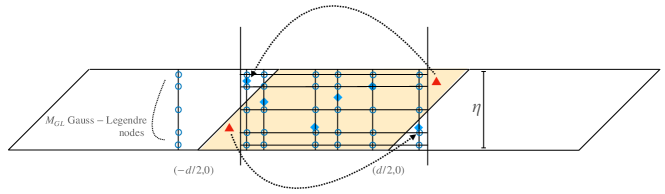
Figure 4: An illustration of the auxiliary grids used for the accelerated algorithm. Blue diamonds represent source locations. We wrap points (red triangles) that fall outside the rectangular box of dimenson $d\times\eta$ (centered at the unit cell center) to their corresponding images within the rectangle. The blue circles are the $M_{\rm GL}$ scaled Gauss-Legendre nodes on $[-\eta/2,\eta/2]$ with the same $x$-coordinates as the original sources themselves. In the first step of the method, we use the adjoint of the one-dimensional interpolation matrix to create fictitious sources whose $x$-coordinate is that of the original source but whose $y$-coordinate is one of the $M_{\rm GL}$ Gauss-Legendre nodes at a cost of $O(N_{S}M_{\rm GL})$ work. The NUFFT then provides a fast algorithm for computing ${\bf R}^{south}{\bf q}$ at a cost of $O(M_{\rm GL}\cdot[(r+N_{S})\log(r+N_{S})])$ work. Likewise, once ${\bf c}={\bf D}^{south}\,{\bf R}^{south}{\bf q}$ is obtained, the NUFFT can be used to evaluate the potential on a tensor-product grid with $x$-coordinates corresponding to target locations and $y$-coordinates given by the $M_{\rm GL}$ Gauss-Legendre nodes. (wrapped to the rectangular cell) at a cost of $O(M_{\rm GL}\cdot[(r+N_{T})\log(r+N_{T})])$ work. Interpolation yields the field at the desired target points at a cost of $O(N_{T}M_{\rm GL})$ work.

7 Numerical results

We have implemented the algorithms described in this paper in Fortran. Our implementation uses the fmm2d library [1] for the free-space FMMs and the finufft package [4, 5] for the NUFFTs. The code is complied using gfortran 9.3.0 with -O3 option. The results shown in this section were obtained on a single core of a laptop with Intel(R) 2.40GH i9-10885H CPU.

We first test the performance of the code in the high accuracy regime. Table 1 shows the results for the modified Helmholtz kernel with precision set to $10^{-12}$. $40,000$ source points are placed in the fundamental unit cell with a uniform random distribution, with $500$ equispaced target points on each side of the unit cell to check the enforcement of periodic conditions. In the table, $A$ is the aspect ratio (Definition 2), $t_{\rm per}$ is the time for applying the periodizing operator, $t_{\rm FMM}$ is the time for the FMM call with sources in the near region $\mathcal{N}$ consisting of $(2m_{0}+1)\times(2n_{0}+1)$ copies of the unit cell. $n_{0}=1$ in the doubly periodic case and $n_{0}=0$ in the singly periodic case. $m_{0}=1,2,$ or $3$, depending on the precise shape of the unit cell. $t_{\rm total}$ is the total computational time and $t_{\rm FMM}^{0}$ is the time required by the free-space FMM, with sources restricted to the fundamental unit cell alone for reference as a lower bound. All times are measured in seconds and the error is the estimated relative $l^{2}$ error in satisfying periodicity (i.e., the potential difference between the right and left sides for the singly periodic case, and the sum of potentials differences in both $x$ and $y$ for the doubly periodic case). $P_{1}$ and $P_{2}$ denote the imposition of periodicty in one or two dimensions, respectively. For the singly periodic case, $m_{0}=1$. That is, the central $3$ cells are include in the near region. For the doubly periodic case, $m_{0}=1$ for the rectangular cell; $m_{0}=2$ for the parallelogram with $\theta=\pi/3$; and $m_{0}=3$ for the parallelogram with $\theta=\pi/6$, where $\theta$ is the angle between ${\hat{\bf e}}_{1}$ and ${\hat{\bf e}}_{2}$. The cost of the periodization step is insensitive to the geometry of the unit cell, since we make use of acceleration with the NUFFT, and a small fraction of the total cost. The FMM for sources in the near region $\mathcal{N}$ is about one to four times more expensive than for the unit cell alone. In our current implemnetation, we simply call the free-space FMM with all near region sources but with targets restricted to the unit cell. A more efficient code could be developed by taking advantage of the fact that the sources in each image cells are identical, as are the corresponding hierarchy of multipole moments. Minor modification of the FMM could reduce the cost to being within a factor of two of the FMM cost for the unit cell alone.

Table 1: Timing results of the periodic FMM for the modified Helmholtz kernel with $\beta=1$ and $40,000$ sources in the unit cell. The requested precision is $\epsilon=10^{-12}$.

${A}$	${t_{\rm per}}$	${t_{\rm FMM}}$	${t_{\rm total}}$	${t_{\rm FMM}^{0}}$	Error
$P_{1}:$  rectangle
1	$0.08$	$1.78$	$1.87$	$1.78$	$0.12\text{\times}{10}^{-12}$
10	$0.08$	$1.95$	$2.03$	$1.61$	$0.69\text{\times}{10}^{-14}$
100	$0.12$	$2.19$	$2.30$	$1.37$	$0.86\text{\times}{10}^{-15}$
1000	$0.48$	$2.88$	$3.36$	$1.35$	$0.16\text{\times}{10}^{-14}$
$P_{2}:$  rectangle
1	$0.18$	$2.45$	$2.63$	$1.69$	$0.31\text{\times}{10}^{-13}$
10	$0.17$	$2.48$	$2.65$	$1.62$	$0.44\text{\times}{10}^{-14}$
100	$0.17$	$3.70$	$3.87$	$1.39$	$0.49\text{\times}{10}^{-15}$
1000	$0.19$	$3.72$	$3.91$	$1.36$	$0.48\text{\times}{10}^{-15}$
$P_{2}:$  parallelogram with  $\theta=\pi/3$
2	$0.18$	$3.40$	$3.59$	$1.82$	$0.20\text{\times}{10}^{-12}$
10	$0.17$	$3.45$	$3.63$	$1.78$	$0.35\text{\times}{10}^{-12}$
100	$0.17$	$4.24$	$4.42$	$1.39$	$0.12\text{\times}{10}^{-12}$
1000	$0.19$	$3.84$	$4.03$	$1.36$	$0.45\text{\times}{10}^{-12}$
$P_{2}:$  parallelogram with  $\theta=\pi/6$
2	$0.18$	$4.18$	$4.37$	$1.53$	$0.17\text{\times}{10}^{-12}$
10	$0.17$	$3.30$	$3.48$	$1.95$	$0.15\text{\times}{10}^{-12}$
100	$0.17$	$4.25$	$4.42$	$1.38$	$0.32\text{\times}{10}^{-12}$
1000	$0.22$	$3.95$	$4.18$	$1.36$	$0.26\text{\times}{10}^{-12}$

Similar results hold for the other kernels. In Table 2 we show the timings obtained for the Laplace kernel with precision $\epsilon=10^{-9}$, and in Table 3, we show the timings obtained for the Stokeslet with precision $\epsilon=10^{-6}$. The column headings have the same meaning as in Table 1.

Table 2: Timing results of the periodic FMM for the Laplace kernel with $40,000$ sources in the unit cell and a requested precision of $\epsilon=10^{-9}$.

${A}$	${t_{\rm per}}$	${t_{\rm FMM}}$	${t_{\rm total}}$	${t_{\rm FMM}^{0}}$	Error
$P_{1}:$  rectangle
1	$0.06$	$0.56$	$0.62$	$0.64$	$0.10\text{\times}{10}^{-09}$
10	$0.07$	$0.83$	$0.90$	$0.66$	$0.98\text{\times}{10}^{-11}$
100	$0.08$	$0.64$	$0.73$	$0.44$	$0.21\text{\times}{10}^{-12}$
1000	$0.23$	$1.02$	$1.25$	$0.40$	$0.15\text{\times}{10}^{-12}$
$P_{2}:$  rectangle
1	$0.14$	$1.03$	$1.17$	$0.54$	$0.11\text{\times}{10}^{-10}$
10	$0.12$	$0.81$	$0.93$	$0.66$	$0.63\text{\times}{10}^{-11}$
100	$0.12$	$1.14$	$1.27$	$0.44$	$0.13\text{\times}{10}^{-11}$
1000	$0.13$	$1.48$	$1.61$	$0.40$	$0.52\text{\times}{10}^{-13}$
$P_{2}:$  parallelogram with  $\theta=\pi/3$
2	$0.14$	$1.13$	$1.27$	$0.65$	$0.26\text{\times}{10}^{-10}$
10	$0.12$	$1.17$	$1.29$	$0.72$	$0.13\text{\times}{10}^{-09}$
100	$0.12$	$1.64$	$1.77$	$0.44$	$0.31\text{\times}{10}^{-09}$
1000	$0.13$	$1.29$	$1.42$	$0.40$	$0.24\text{\times}{10}^{-09}$
$P_{2}:$  parallelogram with  $\theta=\pi/6$
2	$0.13$	$1.76$	$1.90$	$0.46$	$0.20\text{\times}{10}^{-10}$
10	$0.13$	$1.11$	$1.24$	$0.62$	$0.23\text{\times}{10}^{-09}$
100	$0.12$	$1.66$	$1.78$	$0.45$	$0.60\text{\times}{10}^{-10}$
1000	$0.13$	$1.28$	$1.42$	$0.40$	$0.34\text{\times}{10}^{-09}$

Table 3: Timing results of the periodic FMM for the Stokeslet with $40,000$ sources in the unit cell and a requested precision of $\epsilon=10^{-6}$.

${A}$	${t_{\rm per}}$	${t_{\rm FMM}}$	${t_{\rm total}}$	${t_{\rm FMM}^{0}}$	Error
$P_{1}:$  rectangle
1	$0.09$	$1.05$	$1.14$	$0.81$	$0.19\text{\times}{10}^{-06}$
10	$0.07$	$1.17$	$1.24$	$0.94$	$0.12\text{\times}{10}^{-06}$
100	$0.08$	$1.09$	$1.18$	$0.78$	$0.16\text{\times}{10}^{-08}$
1000	$0.19$	$1.31$	$1.50$	$0.69$	$0.39\text{\times}{10}^{-10}$
$P_{2}:$  rectangle
1	$0.25$	$1.63$	$1.89$	$0.69$	$0.21\text{\times}{10}^{-07}$
10	$0.24$	$1.31$	$1.55$	$0.94$	$0.53\text{\times}{10}^{-07}$
100	$0.23$	$1.42$	$1.65$	$0.79$	$0.73\text{\times}{10}^{-08}$
1000	$0.24$	$2.30$	$2.55$	$0.69$	$0.12\text{\times}{10}^{-09}$
$P_{2}:$  parallelogram with  $\theta=\pi/3$
2	$0.25$	$1.50$	$1.75$	$0.78$	$0.35\text{\times}{10}^{-07}$
10	$0.24$	$1.55$	$1.80$	$0.88$	$0.19\text{\times}{10}^{-06}$
100	$0.24$	$2.30$	$2.55$	$0.80$	$0.57\text{\times}{10}^{-06}$
1000	$0.25$	$2.31$	$2.56$	$0.69$	$0.39\text{\times}{10}^{-06}$
$P_{2}:$  parallelogram with  $\theta=\pi/6$
2	$0.25$	$2.24$	$2.50$	$0.88$	$0.72\text{\times}{10}^{-07}$
10	$0.24$	$1.58$	$1.83$	$0.77$	$0.47\text{\times}{10}^{-06}$
100	$0.24$	$2.29$	$2.53$	$0.82$	$0.32\text{\times}{10}^{-06}$
1000	$0.25$	$2.27$	$2.52$	$0.68$	$0.61\text{\times}{10}^{-06}$

8 Conclusions

Explicit, separable low-rank factorizations have been constructed for the periodizing operator for particle interactions governed by the modified Helmholtz, Poisson, modified Stokes, and Stokes equations in two dimensions. The factorization is based on the Sommerfeld integral representation of the Green’s function, which is readily available for the modified Helmholtz and Poisson kernels, and can be derived more generally by Fourier analysis and contour integration, as done here for the modified Stokeslet or Stokeslet. In both the singly and doubly periodic cases, the $\epsilon$-rank $r$ of the periodizing operator is shown to be of the order $O\left(\log(1/\epsilon)\left(\log(1/\beta)+A\log(1/\epsilon)\right)\right)$, where $A$ is the aspect ratio of the fundamental unit cell. Here, $\beta$ is the parameter that defines the modified Helmholtz and modified Stokes kernels. For the Poisson and Stokes kernels, the factor $\log(1/\beta)$ disappears.

Our factorization leads to a simple fast algorithm for the action of the periodizing operators with $O(r(N_{T}+N_{S}))$ complexity - linear with respect to the number of targets and sources. When $r$ is large, a more complicated fast algorithm, relying on the NUFFT, can be used to further speed up the calculation, reducing the complexity to $O(\log(1/\epsilon)(r\log r+(N_{T}+N_{S})\log(1/\epsilon)))$.

There are several natural extensions or generalizations of the current work. First, the scheme can easily be extended to treat nonoscillatory kernels in three dimensions. Second, there is no essential obstacle to extending the scheme to treat oscillatory problems (such as the Helmholtz or Maxwell equations) in two and three dimensions. The various sums and integrals, however, must be treated with more care, as they are conditionally convergent, permit “quasi-periodic” boundary conditions and are subject to resonances (Wood anomalies) [2, 3, 12, 13, 17, 34]. Third, the scheme can be coupled with integral equation methods and the fast multipole method to solve periodic boundary value problems when the unit cell contains inclusions of complicated shape. Finally, more efficient versions of the FMM can be deployed to reduce the cost of handling the near region copies of the unit cell, as in the periodic version of the original scheme [23]. This would bring into closer alignment the time ${t_{\rm FMM}}$ and ${t_{\rm FMM}^{0}}$ in Tables 1, 2 and 3. For multiple scattering problems with singly or doubly periodic boundary conditions, where the far field of a scatterer is represented by a multipole expansion, the periodic scattering matrix can be constructed via simple modifications of the algorithms in [20, 21]. This requires periodizing operators for multipole sources, which are presented in the appendices of the present paper.

Appendix A Rotated plane-wave expansions for the east and west parts of the doubly periodic periodizing operators

In the analysis and implementation of the present paper, we have relied on plane-wave expansions that decay in $x$: either for $x>0$ (the west part) or for $x<0$ (the east part). Simple geometric considerations led to the conclusion that we may need to exclude the central $7\times 3$ copies of the unit cell. For non-rectangualr unit cells, it is actually more efficient to align the decay direction in the plane-wave expansion with ${\hat{\bf e}}_{2}^{\perp}$ - that is, orthogonal to the ${\hat{\bf e}}_{2}$ direction. We illustrate the corresponding algorithm in the case of the modified Helmholtz kernel. Consider the coordinate transformation

$$\begin{pmatrix}{\tilde{x}}\\ {\tilde{y}}\end{pmatrix}=\begin{pmatrix}\cos\theta&-\sin\theta\\ \sin\theta&\cos\theta\end{pmatrix}\begin{pmatrix}x\\ y\end{pmatrix}.$$ (88)

In complex notation, this is equivalent to

$${\tilde{x}}+i{\tilde{y}}=e^{i\theta}(x+iy).$$ (89)

Let us also write

$${\tilde{\xi}}+{\tilde{\eta}}=e^{i\theta}(\xi+i\eta),\quad{\tilde{d}}_{x}+i{\tilde{d}}_{y}=de^{i\theta}.$$ (90)

For the west part, if the plane-wave expansion along the ${\tilde{x}}$ direction is used, we have

$$K_{2}^{west}({\bf t},{\bf s}) =\frac{1}{2\pi}\sum_{m=-\infty}^{-(m_{0}+1)}\sum_{n=-1}^{1}K_{0}\left({\bf t},{\bf s}+{\bf l}_{mn}\right)$$ (91)

$$=\sum_{m=-\infty}^{-(m_{0}+1)}\sum_{n=-1}^{1}\int_{-\infty}^{\infty}\frac{e^{-\sqrt{\lambda^{2}+\beta^{2}}({\tilde{x}}-{\tilde{x}}^{\prime}-m{\tilde{d}}_{x}-n{\tilde{\xi}})}}{4\pi\sqrt{\lambda^{2}+\beta^{2}}}\cdot e^{i\lambda({\tilde{y}}-{\tilde{y}}^{\prime}-m{\tilde{d}}_{y}-n{\tilde{\eta}})}d\lambda$$

$$=\sum_{n=-1}^{1}\int_{-\infty}^{\infty}\frac{e^{-\sqrt{\lambda^{2}+\beta^{2}}({\tilde{x}}-{\tilde{x}}^{\prime}-n{\tilde{\xi}})}}{4\pi\sqrt{\lambda^{2}+\beta^{2}}}\cdot e^{i\lambda({\tilde{y}}-{\tilde{y}}^{\prime}-n{\tilde{\eta}})}\frac{e^{-(m_{0}+1)\left(\sqrt{\lambda^{2}+\beta^{2}}{\tilde{d}}_{x}-i\lambda{\tilde{d}}_{y}\right)}}{1-e^{-\left(\sqrt{\lambda^{2}+\beta^{2}}{\tilde{d}}_{x}-i\lambda{\tilde{d}}_{y}\right)}}d\lambda.$$

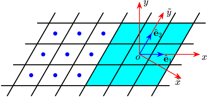
Figure 5: New direction of the plane-wave expansion for the west part. In the main text, we have chosen the plane-wave expansions along the coordinate axes for all four parts. The advantage is that the east and west parts of the doubly periodic periodizing operators can be discretized via efficient precomputed generalized Gaussian quadrature. But the worst case requires the exclusion of the center $7\times 3$ cells from the periodizing operators. If we choose the plane-wave expansion along the $\tilde{x}$-axis, then one only needs to exclude the center $3\times 3$ cells from the doubly periodic periodizing operators. But the number of plane waves may increase if the angle between ${\hat{\bf e}}_{1}$ and ${\hat{\bf e}}_{2}$ is very small and $|{\hat{\bf e}}_{2}|$ is very close to $|{\hat{\bf e}}_{1}|$.

It is now clear that if we choose ${\bf e}_{{\tilde{x}}}={\hat{\bf e}}_{2}^{\perp}$ - that is, we choose $\theta$ such that ${\tilde{\xi}}=0$ and ${\tilde{d}}_{x}>0$, then $m_{0}=1$ is sufficient to ensure that the decaying exponential in the integrand decays at least as fast as $e^{-\sqrt{\lambda^{2}+\beta^{2}}{\tilde{d}}_{x}}$. Thus, one only needs to exclude the center $3\times 3$ cells from the periodizing operator rather than the larger near region we have used above. The integrand could still be highly oscillatory, so that an effective high-order quadrature is needed, just as in singly periodic case.

Appendix B Periodizing operators for the modified Helmholtz equation with multipole sources

The multipole of order $l$ for the modified Helmholtz multipole is defined by $K_{l}(\beta r)e^{il\theta}$, where $K_{l}$ the modified Bessel function of the second kind of order $l$. The following lemma describes the corresponding plane-wave expansions for the far-field contributions of the periodizing operators.

Lemma 1.

For the standard unit cell $\mathcal{C}$ discussed in the main text, let $K_{2}^{south}$, $K_{2}^{north}$, $K_{2}^{west}$, $K_{2}^{east}$ denote the far-field parts of the periodizing operator for a multipole source of order $l$ governed by the modified Helmholtz equation subject to doubly periodic boundary conditions. That is,

$$K_{2}^{south}({\bf t},{\bf s}) =\sum_{n=-\infty}^{-2}\sum_{m=-\infty}^{\infty}K_{l}({\bf t},{\bf s}+{\bf l}_{mn})e^{il\theta_{mn}},$$ (92)

$$K_{2}^{north}({\bf t},{\bf s}) =\sum_{n=2}^{\infty}\sum_{m=-\infty}^{\infty}K_{l}({\bf t},{\bf s}+{\bf l}_{mn})e^{il\theta_{mn}},$$

$$K_{2}^{west}({\bf t},{\bf s}) =\sum_{n=-1}^{1}\sum_{m=-\infty}^{-4}K_{l}({\bf t},{\bf s}+{\bf l}_{mn})e^{il\theta_{mn}},$$

$$K_{2}^{east}({\bf t},{\bf s}) =\sum_{n=-1}^{1}\sum_{m=4}^{\infty}K_{l}({\bf t},{\bf s}+{\bf l}_{mn})e^{il\theta_{mn}}.$$

Let $\alpha_{m}$, $\chi_{m}$ and $Q_{m}$ be given by Eq. 28. Then

$$K_{2}^{south}({\bf t},{\bf s}) =\frac{\pi i^{l}}{d}\sum_{m=-\infty}^{\infty}\left(\frac{\beta}{\chi_{m}+\alpha_{m}}\right)^{l}\frac{1}{\chi_{m}}e^{-\chi_{m}(y-y^{\prime})+i\alpha_{m}(x-x^{\prime})}\frac{e^{-2Q_{m}}}{1-e^{-Q_{m}}}\,,$$ (93)

$$K_{2}^{north}({\bf t},{\bf s}) =\frac{\pi(-i)^{l}}{d}\sum_{m=-\infty}^{\infty}\left(\frac{\chi_{m}+\alpha_{m}}{\beta}\right)^{l}\frac{1}{\chi_{m}}e^{\chi_{m}(y-y^{\prime})+i\alpha_{m}(x-x^{\prime})}\frac{e^{-2\overline{Q_{m}}}}{1-e^{-\overline{Q_{m}}}}\,,$$

$$K_{2}^{west}({\bf t},{\bf s}) =\frac{1}{2\beta^{l}}\sum_{n=-1}^{1}\int_{-\infty}^{\infty}\left(\sqrt{\lambda^{2}+\beta^{2}}+\lambda\right)^{l}\frac{e^{-\sqrt{\lambda^{2}+\beta^{2}}(x-x^{\prime}-n\xi)}}{\sqrt{\lambda^{2}+\beta^{2}}}$$

$$\cdot e^{i\lambda(y-y^{\prime}-n\eta)}\frac{e^{-4\sqrt{\lambda^{2}+\beta^{2}}d}}{1-e^{-\sqrt{\lambda^{2}+\beta^{2}}d}}d\lambda\,,$$

$$K_{2}^{east}({\bf t},{\bf s}) =\frac{(-1)^{l}}{2\beta^{l}}\sum_{n=-1}^{1}\int_{-\infty}^{\infty}\left(\sqrt{\lambda^{2}+\beta^{2}}-\lambda\right)^{l}\frac{e^{\sqrt{\lambda^{2}+\beta^{2}}(x-x^{\prime}-n\xi)}}{\sqrt{\lambda^{2}+\beta^{2}}}$$

$$\cdot e^{i\lambda(y-y^{\prime}-n\eta)}\frac{e^{-4\sqrt{\lambda^{2}+\beta^{2}}d}}{1-e^{-\sqrt{\lambda^{2}+\beta^{2}}d}}d\lambda\,.$$

Similarly, for the singly periodic case,

$$K_{1}^{west}({\bf t},{\bf s}) =\sum_{m=-\infty}^{-2}K_{l}({\bf t},{\bf s}+(md,0))e^{il\theta_{m0}},$$ (94)

$$=\frac{1}{2\beta^{l}}\int_{-\infty}^{\infty}\left(\sqrt{\lambda^{2}+\beta^{2}}+\lambda\right)^{l}\frac{e^{-\sqrt{\lambda^{2}+\beta^{2}}(x-x^{\prime})}}{\sqrt{\lambda^{2}+\beta^{2}}}$$

$$\cdot e^{i\lambda(y-y^{\prime})}\frac{e^{-2\sqrt{\lambda^{2}+\beta^{2}}d}}{1-e^{-\sqrt{\lambda^{2}+\beta^{2}}d}}d\lambda\,,$$

$$K_{1}^{east}({\bf t},{\bf s}) =\sum_{m=2}^{\infty}K_{l}({\bf t},{\bf s}+(md,0))e^{il\theta_{m0}}$$

$$=\frac{(-1)^{l}}{2\beta^{l}}\int_{-\infty}^{\infty}\left(\sqrt{\lambda^{2}+\beta^{2}}-\lambda\right)^{l}\frac{e^{\sqrt{\lambda^{2}+\beta^{2}}(x-x^{\prime})}}{\sqrt{\lambda^{2}+\beta^{2}}}$$

$$\cdot e^{i\lambda(y-y^{\prime})}\frac{e^{-2\sqrt{\lambda^{2}+\beta^{2}}d}}{1-e^{-\sqrt{\lambda^{2}+\beta^{2}}d}}d\lambda\,.$$

The preceding result yields the following low-rank decompositions for the periodizing operators.

Lemma 2.

Under the hypotheses of Theorem 1 and Theorem 3, let

$${\bf L}^{south},{\bf L}^{north}\in\mathbb{C}^{N_{T}\times(2M+1)}$$

and ${\bf R}^{south},{\bf R}^{north}\in\mathbb{C}^{(2M+1)\times N_{S}}$ be dense matrices defined in Eqs. 29 and 36, and let ${\bf L}_{1}^{west}\in\mathbb{C}^{N_{T}\times 2N^{1}_{q}}$, ${\bf L}_{2}^{west}\in\mathbb{C}^{N_{T}\times 2N^{2}_{q}}$, ${\bf R}_{1}^{west}\in\mathbb{C}^{2N^{1}_{q}\times N_{S}}$, ${\bf R}_{2}^{west}\in\mathbb{C}^{2N^{2}_{q}\times N_{S}}$ be dense matrices defined in Eq. 40. Furthermore, let ${\bf D}^{south},{\bf D}^{north}\in\mathbb{C}^{(2M+1)\times(2M+1)}$ be diagonal matrices with

$${\bf D}^{south}(m,m) =\frac{\pi i^{l}}{d}\left(\frac{\beta}{\chi_{m}+\alpha_{m}}\right)^{l}\frac{1}{\chi_{m}}\frac{e^{-2Q_{m}}}{1-e^{-Q_{m}}}\,,$$ (95)

$${\bf D}^{north}(m,m) =\frac{\pi(-i)^{l}}{d}\left(\frac{\chi_{m}+\alpha_{m}}{\beta}\right)^{l}\frac{1}{\chi_{m}}\frac{e^{-2\overline{Q_{m}}}}{1-e^{-\overline{Q_{m}}}}\,,$$

and let ${\bf D}_{1}^{west},{\bf D}_{1}^{east}$, and ${\bf D}_{2}^{west}$, ${\bf D}_{2}^{east}$ be diagonal matrices of dimension $2N^{1}_{q}$ and $2N^{2}_{q}$, respectively, with

$${\bf D}_{1}^{west}(n,n) =\frac{1}{2\beta^{l}}\left(\sqrt{\lambda_{n,1}^{2}+\beta^{2}}+\lambda_{n,1}\right)^{l}\frac{w_{n,1}}{\sqrt{\lambda_{n,1}^{2}+\beta^{2}}}\frac{e^{-2\sqrt{\lambda_{n,1}^{2}+\beta^{2}}d}}{1-e^{-\sqrt{\lambda_{n,1}^{2}+\beta^{2}}d}}\,,$$ (96)

$${\bf D}_{1}^{east}(n,n) =\frac{(-1)^{l}}{2\beta^{l}}\left(\sqrt{\lambda_{n,1}^{2}+\beta^{2}}-\lambda_{n,1}\right)^{l}\frac{w_{n,1}}{\sqrt{\lambda_{n,1}^{2}+\beta^{2}}}\frac{e^{-2\sqrt{\lambda_{n,1}^{2}+\beta^{2}}d}}{1-e^{-\sqrt{\lambda_{n,1}^{2}+\beta^{2}}d}}\,,$$

$${\bf D}_{2}^{west}(n,n) =\frac{1}{2\beta^{l}}\left(\sqrt{\lambda_{n,2}^{2}+\beta^{2}}+\lambda_{n,2}\right)^{l}\frac{w_{n,2}}{\sqrt{\lambda_{n,2}^{2}+\beta^{2}}}\frac{e^{-4\sqrt{\lambda_{n,2}^{2}+\beta^{2}}d}}{1-e^{-\sqrt{\lambda_{n,2}^{2}+\beta^{2}}d}}$$

$$\cdot[e^{-\sqrt{\lambda_{n,2}^{2}+\beta^{2}}\xi+i\lambda_{n,2}\eta}+e^{\sqrt{\lambda_{n,2}^{2}+\beta^{2}}\xi-i\lambda_{n,2}\eta}+1]\,,$$

$${\bf D}_{2}^{east}(n,n) =\frac{(-1)^{l}}{2\beta^{l}}\left(\sqrt{\lambda_{n,2}^{2}+\beta^{2}}-\lambda_{n,2}\right)^{l}\frac{w_{n,2}}{\sqrt{\lambda_{n,2}^{2}+\beta^{2}}}\frac{e^{-4\sqrt{\lambda_{n,2}^{2}+\beta^{2}}d}}{1-e^{-\sqrt{\lambda_{n,2}^{2}+\beta^{2}}d}}$$

$$\cdot[e^{-\sqrt{\lambda_{n,2}^{2}+\beta^{2}}\xi-i\lambda_{n,2}\eta}+e^{\sqrt{\lambda_{n,2}^{2}+\beta^{2}}\xi+i\lambda_{n,2}\eta}+1]\,,$$

where $\lambda_{-n,1}=-\lambda_{n,1}$ for $n=1,\ldots,N_{q}^{1}$, and $\lambda_{-n,2}=-\lambda_{n,2}$ for $n=1,\ldots,N_{q}^{2}$. Then, the periodizing operators for the modified Helmholtz multipole of order $l$ are given by

$${\bf P}_{2}^{south} ={\bf L}^{south}\,{\bf D}^{south}\,{\bf R}^{south}+O(\epsilon),$$ (97)

$${\bf P}_{2}^{north} ={\bf L}^{north}\,{\bf D}^{north}\,{\bf R}^{north}+O(\epsilon),$$

$${\bf P}_{2}^{west} ={\bf L}_{2}^{west}\,{\bf D}_{2}^{west}\,{\bf R}_{2}^{west}+O(\epsilon),$$

$${\bf P}_{2}^{east} ={\bf L}_{2}^{east}\,{\bf D}_{2}^{east}\,{\bf R}_{2}^{east}+O(\epsilon),$$

$${\bf P}_{1}^{west} ={\bf L}_{1}^{west}\,{\bf D}_{1}^{west}\,{\bf R}_{1}^{west}+O(\epsilon),$$

$${\bf P}_{1}^{east} ={\bf L}_{1}^{east}\,{\bf D}_{1}^{east}\,{\bf R}_{1}^{east}+O(\epsilon).$$

Appendix C Periodizing operators for the Laplace equation with multipole sources

In two dimensions, using complex variables notation, the Laplace multipole of order $l$ is simply $1/z^{l}$. Here we identify ${\bf t}$ with $z=x+iy$, ${\bf s}$ with $z^{\prime}=x^{\prime}+iy^{\prime}$, ${\hat{\bf e}}_{1}$ with $e_{1}=d$, ${\hat{\bf e}}_{2}$ with $e_{2}=\xi+i\eta$, and ${\bf l}_{mn}$ with $z_{mn}=m\cdot e_{1}+n\cdot e_{2}$. The following lemma contains the plane-wave expansions for the far-field parts of the corresponding periodic kernels.

Lemma 3.

For the standard unit cell $\mathcal{C}$ discussed in the main text, let $K_{2}^{south}$, $K_{2}^{north}$, $K_{2}^{west}$, $K_{2}^{east}$ denote the far-field parts of the periodizing operator for a multipole source of order $l$ governed by the Laplace equation subject to doubly periodic boundary conditions. That is,

$$K_{2}^{south}({\bf t},{\bf s}) =\sum_{n=-\infty}^{-2}\sum_{m=-\infty}^{\infty}\frac{1}{(z-z^{\prime}-z_{mn})^{l}},$$ (98)

$$K_{2}^{north}({\bf t},{\bf s}) =\sum_{n=2}^{\infty}\sum_{m=-\infty}^{\infty}\frac{1}{(z-z^{\prime}-z_{mn})^{l}},$$

$$K_{2}^{west}({\bf t},{\bf s}) =\sum_{n=-1}^{1}\sum_{m=-\infty}^{-4}\frac{1}{(z-z^{\prime}-z_{mn})^{l}},$$

$$K_{2}^{east}({\bf t},{\bf s}) =\sum_{n=-1}^{1}\sum_{m=4}^{\infty}\frac{1}{(z-z^{\prime}-z_{mn})^{l}}.$$

Let $Q_{m}=2\pi m(\eta-i\xi)/d$. Then

$$K_{2}^{south}({\bf t},{\bf s}) =\frac{(-2\pi i)^{l}}{(l-1)!d^{l}}\,\sum_{m=1}^{\infty}m^{l-1}e^{i\frac{2\pi m}{d}(z-z^{\prime})}\frac{e^{-2Q_{m}}}{1-e^{-Q_{m}}}+\delta_{l1}\frac{\pi i}{d\eta}y,$$ (99)

$$K_{2}^{north}({\bf t},{\bf s}) =\frac{(2\pi i)^{l}}{(l-1)!d^{l}}\,\sum_{m=1}^{\infty}m^{l-1}e^{-i\frac{2\pi m}{d}(z-z^{\prime})}\frac{e^{-2\overline{Q_{m}}}}{1-e^{-\overline{Q_{m}}}}+\delta_{l1}\frac{\pi i}{d\eta}y,$$

$$K_{2}^{west}({\bf t},{\bf s}) =\frac{1}{(l-1)!}\,\int_{0}^{\infty}\lambda^{l-1}\left(1+e^{\lambda\cdot e_{2}}+e^{-\lambda\cdot e_{2}}\right)e^{-\lambda(z-z^{\prime})}\frac{e^{-4\lambda d}}{1-e^{-\lambda d}}d\lambda,$$

$$K_{2}^{east}({\bf t},{\bf s}) =\frac{(-1)^{l}}{(l-1)!}\,\int_{0}^{\infty}\lambda^{l-1}\left(1+e^{\lambda\cdot e_{2}}+e^{-\lambda\cdot e_{2}}\right)e^{\lambda(z-z^{\prime})}\frac{e^{-4\lambda d}}{1-e^{-\lambda d}}d\lambda.$$

Similarly, for the singly periodic case,

$$K_{1}^{west}({\bf t},{\bf s}) =\sum_{m=-\infty}^{-2}\frac{1}{(z-z^{\prime}-z_{mn})^{l}}$$ (100)

$$=\frac{1}{(l-1)!}\,\int_{0}^{\infty}\lambda^{l-1}e^{-\lambda(z-z^{\prime})}\frac{e^{-2\lambda d}}{1-e^{-\lambda d}}d\lambda,$$

$$K_{1}^{east}({\bf t},{\bf s}) =\sum_{m=2}^{\infty}\frac{1}{(z-z^{\prime}-z_{mn})^{l}}$$

$$=\frac{(-1)^{l}}{(l-1)!}\,\int_{0}^{\infty}\lambda^{l-1}e^{\lambda(z-z^{\prime})}\frac{e^{-2\lambda d}}{1-e^{-\lambda d}}d\lambda.$$

The derivation of the associated periodizing operators is straightforward and omitted. Note that the integrals in Eq. 99 and Eq. 100 diverge at the origin when $l=1$, but the divergence is compensated for in the associated periodizing operators under the assumption of charge neutrality.

Appendix D Periodizing operators for the Stokes stresslet

The stresslet for the Stokes equation is defined by the formula

$$T^{(S)}_{ijk}({\bf t},{\bf s})=\frac{\partial G^{(S)}_{ij}({\bf t},{\bf s})}{\partial x_{k}}+\frac{\partial G^{(S)}_{jk}({\bf t},{\bf s})}{\partial x_{i}}-p_{j}({\bf t},{\bf s})\delta_{jk},$$ (101)

where $G^{(S)}_{ij}$ is the $ij$-th component of the Stokeslet in Eq. 69, $p_{j}$ is the $j$th component of the pressurelet in Eq. 80, and the partial derivatives are with respect to the source point ${\bf s}$. It is inconvenient to write down the periodizing operators for the stresslet due to its tensor structure. In practice, it is often combined with a vector ${\bf n}$ to form the kernel of the double layer potential operator or its adjoint operator, when ${\bf n}=(n_{1},n_{2})$ is the unit normal vector at the source point ${\bf s}$ or the target point ${\bf t}$, respectively. Thus, we will write down the periodizing operators for the kernel ${\bf D}^{(S)}$ of the double layer potential operator defined by the formula $D^{(S)}_{ij}=T^{(S)}_{jik}n_{k}$ instead.

Lemma 4.

For the standard unit cell $\mathcal{C}$ discussed in the main text, let $K_{2}^{south}$, $K_{2}^{north}$, $K_{2}^{west}$, $K_{2}^{east}$ denote the far-field parts of the periodizing operator for the kernel of the Stokes double layer potential subject to doubly periodic boundary conditions. That is,

$$K_{2}^{south}({\bf t},{\bf s}) =\sum_{n=-\infty}^{-2}\sum_{m=-\infty}^{\infty}{\bf D}^{(S)}({\bf t},{\bf s}+{\bf l}_{mn}),$$ (102)

$$K_{2}^{north}({\bf t},{\bf s}) =\sum_{n=2}^{\infty}\sum_{m=-\infty}^{\infty}{\bf D}^{(S)}({\bf t},{\bf s}+{\bf l}_{mn}),$$

$$K_{2}^{west}({\bf t},{\bf s}) =\sum_{n=-1}^{1}\sum_{m=-\infty}^{-4}{\bf D}^{(S)}({\bf t},{\bf s}+{\bf l}_{mn}),$$

$$K_{2}^{east}({\bf t},{\bf s}) =\sum_{n=-1}^{1}\sum_{m=4}^{\infty}{\bf D}^{(S)}({\bf t},{\bf s}+{\bf l}_{mn}).$$

Let $\alpha_{m}=2\pi m/d$ and $Q_{m}=2\pi m(\eta-i\xi)/d$. Then

$${\bf K}_{2}^{south}({\bf t},{\bf s}) =\frac{y}{2d\eta}\begin{bmatrix}n_{2}&n_{1}\\ n_{1}&n_{2}\end{bmatrix}+\frac{1}{2d}\sum_{\begin{subarray}{c}m=-\infty\\ m\neq 0\end{subarray}}^{\infty}\left\{\begin{bmatrix}2i\operatorname{sign}(m)n_{1}-n_{2}&-n_{1}\\ -n_{1}&-n_{2}\end{bmatrix}\right.$$ (103)

$$\left.-(i\alpha_{m}n_{1}-|\alpha_{m}|n_{2})\left(y-y^{\prime}+\frac{2-e^{-Q_{m}}}{1-e^{-Q_{m}}}\eta\right)\begin{bmatrix}1&i\operatorname{sign}(m)\\ i\operatorname{sign}(m)&-1\end{bmatrix}\right\}$$

$$\qquad\qquad\qquad\cdot\frac{e^{-2Q_{m}}}{1-e^{-Q_{m}}}e^{-|\alpha_{m}|(y-y^{\prime})+i\alpha_{m}(x-x^{\prime})},$$

$${\bf K}_{2}^{north}({\bf t},{\bf s}) =\frac{y}{2d\eta}\begin{bmatrix}n_{2}&n_{1}\\ n_{1}&n_{2}\end{bmatrix}+\frac{1}{2d}\sum_{\begin{subarray}{c}m=-\infty\\ m\neq 0\end{subarray}}^{\infty}\left\{\begin{bmatrix}2i\operatorname{sign}(m)n_{1}+n_{2}&n_{1}\\ n_{1}&n_{2}\end{bmatrix}\right.$$

$$\left.-(i\alpha_{m}n_{1}+|\alpha_{m}|n_{2})\left(y-y^{\prime}-\frac{2-e^{-\overline{Q_{m}}}}{1-e^{-\overline{Q_{m}}}}\eta\right)\begin{bmatrix}-1&i\operatorname{sign}(m)\\ i\operatorname{sign}(m)&1\end{bmatrix}\right\}$$

$$\qquad\qquad\qquad\cdot\frac{e^{-2\overline{Q_{m}}}}{1-e^{-\overline{Q_{m}}}}e^{|\alpha_{m}|(y-y^{\prime})+i\alpha_{m}(x-x^{\prime})},$$

$${\bf K}_{2}^{west}({\bf t},{\bf s}) =\frac{1}{4\pi}\sum_{n=-1}^{1}\int_{-\infty}^{\infty}\frac{e^{-4|\lambda|d}}{1-e^{-|\lambda|d}}e^{-|\lambda|(x-x^{\prime}-n\xi)}e^{i\lambda(y-y^{\prime}-n\eta)}\cdot\left\{\begin{bmatrix}-n_{1}&-n_{2}\\ -n_{2}&-n_{1}+2i\operatorname{sign}(\lambda)n_{2}\end{bmatrix}\right.$$ (104)

$$\left.-(-|\lambda|n_{1}+i\lambda n_{2})\left(x-x^{\prime}-n\xi+\frac{4-3e^{-|\lambda|d}}{1-e^{-|\lambda|d}}d\right)\begin{bmatrix}-1&i\operatorname{sign}(\lambda)\\ i\operatorname{sign}(\lambda)&1\end{bmatrix}\right\}d\lambda,$$

$${\bf K}_{2}^{east}({\bf t},{\bf s}) =\frac{1}{4\pi}\sum_{n=-1}^{1}\int_{-\infty}^{\infty}\frac{e^{-4|\lambda|d}}{1-e^{-|\lambda|d}}e^{|\lambda|(x-x^{\prime}-n\xi)}e^{i\lambda(y-y^{\prime}-n\eta)}\cdot\left\{\begin{bmatrix}n_{1}&n_{2}\\ n_{2}&n_{1}+2i\operatorname{sign}(\lambda)n_{2}\end{bmatrix}\right.$$

$$\left.-(|\lambda|n_{1}+i\lambda n_{2})\left(x-x^{\prime}-n\xi-\frac{4-3e^{-|\lambda|d}}{1-e^{-|\lambda|d}}d\right)\begin{bmatrix}1&i\operatorname{sign}(\lambda)\\ i\operatorname{sign}(\lambda)&-1\end{bmatrix}\right\}d\lambda.$$

Similarly, for singly periodic case,

$${\bf K}_{1}^{west}({\bf t},{\bf s}) =\sum_{m=-\infty}^{-2}{\bf D}^{(S)}({\bf t},{\bf s}+{\bf l}_{m0}),$$ (105)

$$=\frac{1}{4\pi}\int_{-\infty}^{\infty}\frac{e^{-2|\lambda|d}}{1-e^{-|\lambda|d}}e^{-|\lambda|(x-x^{\prime})}e^{i\lambda(y-y^{\prime})}\cdot\left\{\begin{bmatrix}-n_{1}&-n_{2}\\ -n_{2}&-n_{1}+2i\operatorname{sign}(\lambda)n_{2}\end{bmatrix}\right.$$

$$\left.-(-|\lambda|n_{1}+i\lambda n_{2})\left(x-x^{\prime}+\frac{2-e^{-|\lambda|d}}{1-e^{-|\lambda|d}}d\right)\begin{bmatrix}-1&i\operatorname{sign}(\lambda)\\ i\operatorname{sign}(\lambda)&1\end{bmatrix}\right\}d\lambda,$$

$${\bf K}_{1}^{east}({\bf t},{\bf s}) =\sum_{m=2}^{\infty}{\bf D}^{(S)}({\bf t},{\bf s}+{\bf l}_{m0}),$$

$$=\frac{1}{4\pi}\int_{-\infty}^{\infty}\frac{e^{-2|\lambda|d}}{1-e^{-|\lambda|d}}e^{|\lambda|(x-x^{\prime})}e^{i\lambda(y-y^{\prime})}\cdot\left\{\begin{bmatrix}n_{1}&n_{2}\\ n_{2}&n_{1}+2i\operatorname{sign}(\lambda)n_{2}\end{bmatrix}\right.$$

$$\left.-(|\lambda|n_{1}+i\lambda n_{2})\left(x-x^{\prime}-\frac{2-e^{-|\lambda|d}}{1-e^{-|\lambda|d}}d\right)\begin{bmatrix}1&i\operatorname{sign}(\lambda)\\ i\operatorname{sign}(\lambda)&-1\end{bmatrix}\right\}d\lambda.$$

References

- [1] T. Askham, Z. Gimbutas, L. Greengard, L. Lu, M. O’Neil, M. Rachh, and V. Rokhlin, fmm2d software library. https://github.com/flatironinstitute/fmm2d, 2021.
- [2] A. Barnett and L. Greengard, A new integral representation for quasi-periodic fields and its application to two-dimensional band structure calculations, Journal of Computational Physics, 229 (2010), pp. 6898–6914.
- [3] , A new integral representation for quasi-periodic scattering problems in two dimensions, BIT Numerical mathematics, 51 (2011), pp. 67–90.
- [4] A. Barnett and J. Magland, Non-uniform fast Fourier transform library of types , , in dimensions , , . https://github.com/ahbarnett/finufft, 2018.
- [5] A. Barnett, J. Magland, and L. af Klinteberg, A parallel non-uniform fast Fourier transform library based on an “exponential of semicircle” kernel, SIAM J. Sci. Comput., 41 (2019), pp. C479–C504.
- [6] A. H. Barnett, G. R. Marple, S. Veerapaneni, and L. Zhao, A unified integral equation scheme for doubly periodic laplace and stokes boundary value problems in two dimensions, Communications on Pure and Applied Mathematics, 71 (2018), pp. 2334–2380.
- [7] C. L. Berman and L. Greengard, A renormalization method for the evaluation of lattice sums, Journal of Mathematical Physics, 35 (1994), pp. 6036–6048.
- [8] F. Bloch, Über die quantenmechanik der elektronen in kristallgittern, Zeitschrift für Physik, 52 (1928), pp. 555–600.
- [9] J. Bremer, Z. Gimbutas, and V. Rokhlin, A nonlinear optimization procedure for generalized Gaussian quadratures, SIAM J. Sci. Comput., 32 (2010), pp. 1761–1788.
- [10] H. Cheng, L. Greengard, and V. Rokhlin, A fast adaptive multipole algorithm in three dimensions, J. Comput. Phys., 155 (1999), pp. 468–498.
- [11] H. Cheng, J. Huang, and T. J. Leiterman, An adaptive fast solver for the modified Helmholtz equation in two dimensions, J. Comput. Phys., 211 (2006), pp. 616–637.
- [12] R. Denlinger, Z. Gimbutas, L. Greengard, and V. Rokhlin, A fast summation method for oscillatory lattice sums, Journal of Mathematical Physics, 58 (2017), p. 023511.
- [13] A. Dienstfrey, F. Hang, and J. Huang, Lattice sums and the two-dimensional, periodic green’s function for the helmholtz equation, Proceedings of the Royal Society of London. Series A: Mathematical, Physical and Engineering Sciences, 457 (2001), pp. 67–85.
- [14] A. Dutt and V. Rokhlin, Fast Fourier transforms for nonequispaced data, SIMA J. Sci. Comput., 14 (1993), pp. 1368–1393.
- [15] , Fast Fourier transforms for nonequispaced data. II, Appl. Comput. Harmon. Anal., 2 (1995), pp. 85–100.
- [16] H. Dym and H. P. McKean, Fourier Series and Integrals, Academic Press, 1972.
- [17] S. Enoch, R. McPhedran, N. Nicorovici, L. Botten, and J. Nixon, Sums of spherical waves for lattices, layers, and lines, Journal of Mathematical Physics, 42 (2001), pp. 5859–5870.
- [18] P. Ewald, Die berechnung optischer und elektrostatischer gitterpotentiale, Annalen der Physik, 64 (1921), pp. 253–287.
- [19] B. Fornberg, A practical guide to pseudospectral methods, vol. 1, Cambridge university press, 1998.
- [20] Z. Gan, S. Jiang, E. Luijten, and Z. Xu, A hybrid method for systems of closely spaced dielectric spheres and ions, SIAM J. Sci. Comput., 38 (2016), pp. B375–B395.
- [21] Z. Gimbutas and L. Greengard, Fast multi-particle scattering: a hybrid solver for the Maxwell equations in microstructured materials, J. Comput. Phys., 232 (2013), pp. 22–32.
- [22] L. Greengard and J. Lee, Accelerating the nonuniform fast Fourier transform, SIAM Rev., 46 (2004), pp. 443–454.
- [23] L. Greengard and V. Rokhlin, A fast algorithm for particle simulations, J. Comput. Phys., 73 (1987), pp. 325–348.
- [24] L. Greengard and V. Rokhlin, A new version of the fast multipole method for the Laplace equation in three dimensions, Acta. Numer., 6 (1997), pp. 229–270.
- [25] J. S. Hesthaven, S. Gottlieb, and D. Gottlieb, Spectral methods for time-dependent problems, vol. 21, Cambridge University Press, 2007.
- [26] T. Hrycak and V. Rokhlin, An improved fast multipole algorithm for potential fields, SIAM J. Sci. Statist. Comput., 19 (1998), pp. 1804–1826.
- [27] J. Huang, Integral representations of harmonic lattice sums, Journal of Mathematical Physics, 40 (1999), pp. 5240–5246.
- [28] D. S. Jones, Generalised functions, McGraw-Hill, New York, 1966.
- [29] J. Lee and L. Greengard, The type 3 nonuniform FFT and its applications, J. Comput. Phys., 206 (2005), pp. 1–5.
- [30] C. M. Linton, Lattice sums for the helmholtz equation, SIAM Review, 52 (2010), pp. 630–674.
- [31] Y. Liu and A. H. Barnett, Efficient numerical solution of acoustic scattering from doubly-periodic arrays of axisymmetric objects, Journal of Computational Physics, 324 (2016), pp. 226–245.
- [32] J. Ma, V. Rokhlin, and S. Wandzura, Generalized Gaussian quadrature rules for systems of arbitrary functions, SIAM J. Numer. Anal., 33 (1996), pp. 971–996.
- [33] D. Malhotra and G. Biros, PVFMM: a parallel kernel independent FMM for particle and volume potentials, Commun. Comput. Phys., 18 (2015), pp. 808–830.
- [34] R. McPhedran, N. Nicorovici, L. Botten, and K. Grubits, Lattice sums for gratings and arrays, Journal of Mathematical Physics, 41 (2000), pp. 7808–7816.
- [35] S. G. Mikhlin and S. Prossdorf, Singular integral operators, Springer–Verlag, Berlin, 1986.
- [36] P. Mores and H. Feshbach, Methods of theoretical physics, McGraw-Hill, New York, 1953.
- [37] A. Moroz, Quasi-periodic Green’s functions of the Helmholtz and Laplace equations, J. Phys. A: Math. Gen., 36 (2006), p. 11247.
- [38] F. W. J. Olver, D. W. Lozier, R. F. Boisvert, and C. W. Clark, eds., NIST Handbook of Mathematical Functions, Cambridge University Press, May 2010.
- [39] Y. Otani and N. Nishimura, A periodic FMM for Maxwell’s equations in 3D and its applications to problems related to photonic crystals, Journal of Computational Physics, 227 (2008), pp. 4630–4652.
- [40] L. Rayleigh, On the influence of obstacles arranged in rectangular order upon the properties of a medium, Philosophical Magazine, 34 (1892), pp. 481–502.
- [41] I. Stakgold, Boundary value problems of mathematical physics, Macmillan, 1968.
- [42] L. N. Trefethen, Is gauss quadrature better than clenshaw–curtis?, SIAM review, 50 (2008), pp. 67–87.
- [43] H. Wang and S. Xiang, On the convergence rates of legendre approximation, Mathematics of Computation, 81 (2012), pp. 861–877.
- [44] J. Wang, E. Nazockdast, and A. Barnett, An integral equation method for the simulation of doubly-periodic suspensions of rigid bodies in a shearing viscous flow, Journal of Computational Physics, 424 (2021), p. 109809.
- [45] W. Yan and M. Shelley, Flexibly imposing periodicity in kernel independent FMM: A multipole-to-local operator approach, Journal of Computational Physics, 335 (2018), pp. 214–232.
- [46] N. Yarvin and V. Rokhlin, Generalized Gaussian quadratures and singular value decompositions of integral operators, SIAM J. Sci. Comput., 20 (1998), pp. 699–718.
- [47] L. Ying, G. Biros, and D. Zorin, A kernel-independent adaptive fast multipole algorithm in two and three dimensions, J. Comput. Phys., 196 (2004), pp. 591–626.