Wave-particle interactions in quantum plasmas

Abstract

Wave-particle interaction (WPI) is one of the most fundamental processes in plasma physics in which one most prominent example is the Landau damping. Owing to its excellent energy-exchange mechanism, the WPI has gained increasing interest not only from theoretical points of view but also its many important applications including plasma heating and plasma acceleration. In this review work, we present theoretical backgrounds of linear and nonlinear wave-particle interactions in quantum plasmas. Specifically, we focus on the wave-particle interactions for homogeneous plasma waves (i.e., waves with infinite extent rather than a localized pulse) as well as for propagating electrostatic waves in the weak and strong quantum regimes to demonstrate the modifications of several classical features including those associated with resonant and trapped particles. Finally, the future perspectives of WPI in quantum plasmas are presented.

1 Introduction

Quantum plasmas have been a topic of important research for nearly sixty years due to their frequent occurrence and potential applications in many astrophysical plasmas (e.g., in the interiors of giant planets like Jupiter, brown and white dwarf stars, and outer crust of neutron stars), in laboratory devices via the compression of matter with lasers, x-rays or ion beams [e.g., the Lawrence Livermore National Laboratory, the Z-machine at Sandia National Laboratory, the Omega laser at the University of Rochester, the European free electron lasers FLASH and X-FEL in Germany and the Linac Coherent Light Source (LCLS) in Stanford], inertial confinement fusion (ICF) plasmas (during the initial phase), quark-gluon plasmas, solid-state plasmas, in semiconductor electron-hole plasmas, as well as in nanoplasmonics which is concerned with the interactions of quantum electrons in metallic nanostructures and electromagnetic radiation haug2009 ; shukla2010 . Quantum plasmas usually consist of different charged particles (e.g., electrons, positrons and protons) in which at least one component is a fermion. In dense plasma environments, the number density of electrons/positrons is extremely high and hence they become degenerate and obey the Fermi-Dirac statistics. We briefly state under what conditions quantum effects start playing a role as follows:

Firstly, according to the Pauli’s exclusion principle, there is at most one fermion in each quantum state, and each occupies a volume $h^{3}$ in phase space. So, the volume per each quantum state of a fermion in real space is $V_{s}=h^{3}/(2\pi mk_{B}T)^{3/2}\sim h^{3}/p^{3}$, i.e., the ratio of the volume in phase space and the volume in momentum space. So, if $n$ is the number of particles per unit volume in phase space, the ratio becomes $nh^{3}/(2\pi mk_{B}T)^{3/2}\sim(T_{F}/T)^{3/2}$, i.e., a parameter $\chi=T_{F}/T$ must be defined to measure the degree of degeneracy of a particle, or to what extent the Pauli’s principle has to be considered. Since $\chi$ can be expressed as $\chi=(1/2)(3\pi^{2})^{2/3}(n\lambda_{B}^{3})^{2/3}$, where $\lambda_{B}=\hbar/mv_{t}$ is the thermal de Broglie wavelength for a fermion (By default, a particle or a fermion means an electron as the same principle applies for other fermions), the quantum degeneracy effect becomes important when $n\lambda_{B}^{3}\geq 1$ and so $\chi\geq 1$. Here, $h=2\pi\hbar$ is the Planck’s constant, $m$ is the electron mass, $T$ is the electron temperature, $k_{B}$ is the Boltzmann constant, $v_{t}=\sqrt{k_{B}T/m}$ is the electron thermal velocity and $T_{F}$ is the Fermi temperature.

Secondly, since the wave function of a particle (electron) with momentum $mv_{t}$ has the wave length $\lambda_{B}$, the quantum effect is expected to be important at length scale $k^{-1}\sim\lambda_{B}$. So, for collective oscillations an important length scale could be such that $(k\lambda_{D})^{-1}\sim\lambda_{B}/\lambda_{D}\sim\hbar\omega_{p}/mv_{t}^{2}\geq 1$, where $\lambda_{D}=v_{t}/\omega_{p}$ is the particle’s Debye length and $\omega_{p}=\sqrt{ne^{2}/\varepsilon_{0}m}$ is the electron plasma frequency in which $e$ is the elementary charge and $\varepsilon_{0}$ is the permittivity of free space. So, another parameter of interest can be defined as $H=\hbar\omega_{p}/mv_{t}^{2}$. For high densities or degenerate electrons $(T_{F}>T)$, $v_{t}$ is to be replaced by the Fermi velocity $v_{F}=\sqrt{k_{B}T_{F}/m}$. Thus, for low density plasmas, $H$ scales as $H\sim n^{1/2}/T$, and for high densities $H\sim n^{-1/6}$. A schematic diagram showing the classical and quantum plasma regimes is shown in Fig. 1

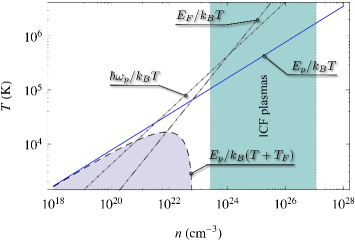
Figure 1: Classical and quantum plasma regimes are shown in the temperature-density parameter space. The figure is reproduced from Ref. zamanian2010 . Each curve represents where the parameter ratios shown are each equal to the unity. The quantum effects become important below either of the lines $E_{F}/k_{B}T=1$ and $\hbar\omega_{p}/k_{B}T=1$. While the ratio $E_{p}/k_{B}T$ denotes the strong coupling parameter in the moderate density regime, $E_{p}/k_{B}(T+T_{F})$ represents that in the high density regime. Here, $E_{F}=k_{B}T_{F}$ is the Fermi energy and $E_{p}=e^{2}n_{0}^{1/3}/4\pi\varepsilon_{0}$ is the potential energy due to the nearest neighbor. The blue shaded part is the region for collisional plasmas.

When plasma particles undergo electrostatic, electromagnetic and quantum forces (e.g., those associated with the statistical pressure, particle spin and exchange-correlation), they oscillate to generate high- or low-frequency electrostatic or electromagnetic waves. Interactions of these waves with fermions provide many interesting and important phenomena occurring in laboratory, space and astrophysical plasmas, as well as in many other environments as mentioned before. For examples, the wave-particle interactions (WPIs) play key roles in the excitation and damping of collective modes, diffusion in velocity space, i.e., thermalization, heating and acceleration of charged particles; transport of particles, momentum and energy. In laboratory, the WPIs can become useful in many important applications including beat wave acceleration, plasma heating in magnetically confined fusion plasmas, edge transport reduction due to magnetic perturbation on multi-scale perturbations, and plasma absorption of laser radiation in inertial fusion experiments antoniazzi2005 . The WPIs in space plasmas occur within the time scales of the plasma gyroperiod or the plasma oscillation period. They can play crucial roles, e.g., in the dynamics of energetic charged particles in the Earth’s Van Allen radiation belts, in the formation of magnetopause boundary layers, precipitation of particles resulting into the formation of auroras, and transport of wave energy from one region to another tsurutani1997 . In astrophysics, the WPI can result into the radiation emission of hard $x$-rays and gamma rays, the stimulated Raman and Brillouin scattering as well as the acceleration of charged particles in relativistic regimes koch2006 . Furthermore, the WPIs in noble-metal nanoparticles can lead to surface-plasmon resonances which have potential applications in nanoscale optics and electronics thakkar2018 . The studies of WPI typically include (i) Coherent WPI, resonance, trapping (ii) Chaos, quasilinear theory, and (iii) Weak and strong turbulence theory. In this article, we will, however, give emphasis on the wave-particle resonance and associated wave damping in relativistic and nonrelativistic quantum plasmas with and without the effects of spin.

One most prominent example of WPIs is the Landau damping. It is the damping of collective modes of oscillations in plasmas without any collision between charged particles. There are, in fact, two approaches to understand the physics of Landau damping: One approach considers the Landau damping in terms of dephasing of charged particles and the other considers Landau damping as the result of energy exchange between waves and particles due to resonance. In this review work, we, however, focus on the second approach. In $1946$, Lev Davidovich Landau first predicted and published a result on plasma oscillations landau1965 . He found that there would be exponential decay of coherent oscillations, i.e., Langmuir wave can suffer damping due to wave-particle interactions. He deduced this effect from a mathematical point of view while solving a Vlasov-Poisson system without its physical explanations. Although correct, the Landau’s derivation was not meticulous from mathematical points of view and later resulted in several conceptual controversies. A number of works were devoted to resolve these issues. To mention few, in $1949$, Bohm and Gross pointed out that the Landau damping results into energy transfer from oscillating coherent field to its resonant particles bohm1949 . Later, in $1955$, Van Kampen kapmen1955 and in $1959$, Case case1959 proved that wave damping can be seen to occur with Fourier transforms and showed that the linearized Vlasov and Poisson equations have a continuous spectrum of singular normal modes. Even after its mathematical verification by Van Kampen kapmen1955 and Case case1959 , and experimental observation by Malmberg and Wharton in $1964$ malmberg1964 , it took almost twenty years to accept the reality of Landau damping.

The subject of wave-particle interactions is very extensive. So, some choices of topics have to be made that can be covered. The paper is organized as follows: In Sec. 2, the linear Landau damping of Langmuir waves is treated starting from the simple classical case, extending the theory to the quantum regime using the Wigner equation, and then finally, covering also the effects of a relativistic background distribution. We start Sec. 3 by reviewing the nonlinear influence on Langmuir wave damping in homogeneous plasmas considering the dynamics in both the weak and strong quantum regimes. Next, we continue with nonlinear generalizations for localized pulse propagation. In particular, we study the nonlinear wave-particle interactions both for ion-acoustic and Langmuir pulses. In the end of Sec. 3, we discuss the wave-particle interactions induced by the electron spin properties. Finally, the review ends with a summary and concluding discussion in Sec. 4.

2 Wave-particle interactions: Linear theory

Wave-particle interaction is a process in which an exchange of energy takes place between waves and particles in a plasma. Such an interaction leads to many interesting phenomena including the scattering and acceleration of particles as well as the growth or damping of waves. The growth (damping) of a wave amplitude occurs depending on whether the wave gains (loses) energy from (to) the particles. In the following sections 2.1 to 2.3, we will mainly focus on wave damping as first described by Landau. In Sec. 2.1, we discuss the basic concept of Landau damping, the Landau’s mathematical treatment to obtain the linear dispersion relation and the damping rate from the Vlasov-Poisson system. The concept of anti-damping or instability is also discussed with some illustrations. We also state the quantum kinetic equations for the description of electrostatic collective oscillations in quantum plasmas. Furthermore, the Landau damping of electrostatic waves in nonrelativistic and relativistic quantum plasmas with different background distributions of electrons is discussed in Secs. 2.2 and 2.3.

2.1 Basic concept of Landau damping

Before we begin with different aspects of wave-particles interactions, especially those of Landau damping, it is pertinent to introduce the basic concept of Landau damping.

2.1.1 Plasma oscillation and wave-particle interaction

We consider an electrically quasi-neutral plasma in equilibrium which consists of mobile electrons and stationary positive ions forming only the background plasma. If electrons are displaced from their equilibrium position, a charge separation occurs and an electric field is created which acts as a restoring force to bring back electrons into their equilibrium position. However, due to their inertia, electrons accelerate towards the equilibrium position and overshoot it in the same way as an oscillating spring does. Thus, a standing wave (Langmuir oscillation) is generated with constant frequency $\omega_{p}$. Note that in the Langmuir oscillation, the individual motion of electrons is not considered. Next, we consider a random motion of electrons (e.g., due to their thermal velocity) with a given velocity distribution for the equilibrium state, and determine under what conditions a wave mode with a wave frequency $\omega$ and wave number $k$ exists. We assume that the oscillating electrons produce electric fields of the following plane wave form with the phase velocity $v_{p}=\omega/k$:

$$E(x,t)=E_{0}\exp[i(kx-\omega t)],$$ (1)

where $E_{0}$ is a constant amplitude of the wave. The oscillating electrons, in turn, interact with the wave electric field they produce leading to the emergence of wave-particle interactions. As a result, the characteristics of particles and hence the field producing the forces are changed. In the wave-particle interaction, since the exchange of energy takes place between waves and particles, either growth (instability) or decay (damping) of the wave amplitude can occur. So, it is reasonable to assume $\omega$ as complex, i.e., $\omega=\omega_{r}+i\gamma$, so that

$$E(x,t)=E_{0}\exp[i(kx-\omega t)]=E_{0}\exp[i(kx-\omega_{r}t)]\exp[\gamma t].$$ (2)

Clearly, the electrostatic oscillation is damped if $\gamma<0$, otherwise for $\gamma>0$ we have an instability or anti-damping. Since particles can have, in general, different velocities, a simple picture is that in a background velocity distribution,

• If more particles move slowly than the wave, particles gain energy from the wave or wave loses energy to the particles, and the wave gets damped.

• If more particles have velocities larger than the wave, wave gains energy from the particles and wave is said to be unstable or anti-damped.

It follows that the slope of the particle’s velocity distribution may become important. However, this picture may not be completely correct. In fact, particles with very different velocities (i.e., much larger or lower than the wave) may not interact with the wave and so, no damping or instability is to occur.

2.1.2 Landau’s mathematical treatment: Classical results

The wave-particle interaction is truly a kinetic phenomena, and so it can not be described by the fluid theory. Landau’s treatment of WPI was based on a Vlasov-Poisson system. In this treatment, the equations for electron plasma oscillations in one-dimension are

$$\frac{\partial f}{\partial t}+v\frac{\partial f}{\partial x}+\frac{e}{m}\frac{\partial\phi}{\partial x}\frac{\partial f}{\partial v}=0,$$ (3)

$$\frac{\partial^{2}\phi}{\partial x^{2}}=\frac{e}{\varepsilon_{0}}\left(\int fdv-n_{0}\right),$$ (4)

where for electrostatic oscillations $E(x,t)=-\partial\phi/\partial x$ is used.

We look for a small amplitude plane wave solution of Eqs. (3) and (4), and accordingly we perturb $f$ and $\phi$ about their equilibrium states as

$$f(x,v,t)=f_{0}(v)+f_{1}(x,v,t),~{}~{}\phi(x,t)=\phi_{1}(x,t).$$ (5)

Thus, instead of considering the Vlasov’s expression as a double Fourier transform, i.e.,

$$f_{1}(x,v,t)=\frac{1}{2\pi}\int_{-\infty}^{\infty}\int_{-\infty}^{\infty}\tilde{f_{1}}(k,v,\omega)e^{i(kx-\omega t)}dkd\omega$$ (6)

and similar for $\phi_{1}$, we consider the Landau’s approach in which the perturbations vary as a Fourier transform in the space domain $(-\infty<x<\infty)$ and a Laplace transform in the time domain $(0<t<\infty)$, i.e.,

$$\tilde{f_{1}}(k,v,t) =\frac{1}{2\pi}\int_{-\infty}^{\infty}f_{1}(x,v,t)e^{ikx}dx,~{}\tilde{\phi_{1}}(k,t)=\frac{1}{2\pi}\int_{-\infty}^{\infty}\phi_{1}(x,t)e^{ikx}dx,$$ (7)

$$f_{1}(k,v,s) =\int_{0}^{\infty}\tilde{f_{1}}(k,v,t)e^{-st}dt,~{}\phi_{1}(k,s)=\int_{0}^{\infty}\phi_{1}(k,t)e^{-st}dt.$$ (8)

Next, linearizing Eqs. (3) and (4) and using Eqs. (7) and (8) we obtain the following dispersion relation for Langmuir waves landau1965 .

$$D(\omega,k)\equiv 1-\frac{\omega_{p}^{2}}{n_{0}k^{2}}\int_{-\infty}^{\infty}\frac{\partial f_{0}/\partial v}{v-\omega/k}dv=0.$$ (9)

From Eq. (9), it is clear that the wave-particle resonance occurs when $v=v_{\text{ph}}\equiv\omega/k$, i.e., when the particle velocity approaches the wave phase velocity. This is called the Landau resonance. A physical picture is that when this resonance condition is satisfied, the particles do not experience a rapidly fluctuating electric field of the wave, i.e., almost a static electric field in the particle’s rest frame, and so they can interact strongly with the wave. Particles near the resonance moving slightly slower (faster) than the wave get accelerated (decelerated) by the wave electric field to move with the wave phase velocity, and hence gain energy from (lose energy to) the wave.

In a collisionless electron-ion plasma with immobile ions and Maxwellian background distribution of electrons there are

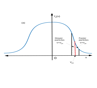
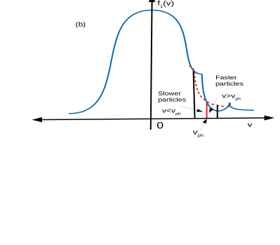
Figure 2: The Landau damping: (a) The initial distribution function $f_{0}(v)$ of electrons and (b) the perturbed distribution function $f_{1}(v)$ after an evolution due to the interaction of background electrons (dashed line) with the wave. The resonance occurs in the region of a negative slope.

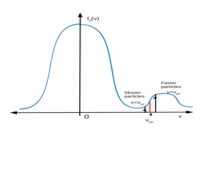
Figure 3: Landau anti-damping (instability): The bump-on-tail distribution function. The resonance occurs in the region of a positive slope.

more slower particles than the faster particles in the negative slope, and so the energy gained from the wave by the slower particles is more than that lost to the wave by the faster particles. As a result, a net wave damping occurs. In order to calculate the wave damping we consider $\omega=\omega_{r}+i\gamma$, assume that the damping is weak, i.e., $|\gamma|\ll\omega_{r}$, and substitute it into the dispersion equation $D(\omega,k)=0$ to obtain

$$D(\omega,k)\equiv D_{r}(\omega_{r},k)+iD_{i}(\omega_{r},k)+i\gamma\frac{\partial D_{r}}{\partial\omega_{r}}=0.$$ (10)

After separating the real and imaginary parts, from Eq. (10) we obtain

$$D(\omega_{r},k)\equiv 1-\frac{\omega_{p}^{2}}{n_{0}k^{2}}{\cal P}\int_{-\infty}^{\infty}\frac{\partial f_{0}/\partial v}{v-\omega_{r}/k}dv=0,$$ (11)

$$\gamma=-\frac{D_{i}(\omega_{r},k)}{\partial D_{r}/\partial\omega_{r}}~{}\rm{with}~{}D_{i}(\omega_{r},k)=-\frac{\pi\omega_{p}^{2}}{n_{0}k^{2}}\left[\frac{\partial f_{0}(v)}{\partial v}\right]_{v=\omega_{r}/k}.$$ (12)

For an one-dimensional Maxwellian background distribution of electrons we have

$$f_{0}(v)=\frac{n_{0}}{\sqrt{2\pi}v_{t}}\exp\left(-v^{2}/2v_{t}^{2}\right).$$ (13)

Figure 2 shows the Landau damping in which subplot (a) is for an initial distribution of thermal electrons with some narrow regions centered at the resonant velocity $v=v_{\text{ph}}$ showing the more slower particles than the fast particles and the subplot (b) shows a perturbed distribution function, i.e., after an evolution due to the interaction of the background distribution of electrons (dashed line) with the wave. Since particles with the velocity $v\approx v_{p}$ are trapped in the wave, this interaction results in the flattening of the distribution function $f_{1}(v)$ around the phase velocity (solid line). However, $f_{1}(v)$ contains the same number of particles which gain the total energy at the expense of the wave. On the other hand, in a non-Maxwellian plasma, if in some region of the phase space, the particle’s distribution has more particles at higher velocities than those with lower velocities [see Fig. 3], then the wave will gain energy from the particles leading to what is known as “bump-on-tail” instability sarkar2015 or inverse Landau damping or Cherenkov instability. Thus, a beam of fast electrons having velocities much higher than their thermal speed will cause Langmuir waves to grow as there are available free energy of electrons. This kind of instability plays an important role, e.g., in solar radio bursts thejappa2018 .

Next, for the Maxwellian background distribution of electrons [Eq. (13)], the classical dispersion relation for Langmuir waves and the Landau damping rate can be obtained from Eqs. (11) and (12). In order that the Langmuir waves are not strongly damped we must have $v_{\text{ph}}>v_{t}$. So, in the non-resonance region assuming $v_{\text{ph}}\gg v$ and keeping terms up to the second-order of $v/v_{\text{ph}}$ in the binomial expansion of $(v-v_{\text{ph}})^{-2}$, we obtain

$$\omega^{2}=\omega_{p}^{2}+3k^{2}v_{t}^{2}\omega_{p}^{2}/\omega^{2}.$$ (14)

If the thermal correction is small then replacing $\omega$ by $\omega_{p}$ (since $\omega=\omega_{p}$ for $v_{t}=0$) we obtain the following dispersion relation for Langmuir waves.

$$\omega^{2}=\omega_{p}^{2}+3k^{2}v_{t}^{2}.$$ (15)

The Landau damping rate is obtained from Eq. (12) as

$$\gamma=-\frac{\sqrt{\pi}}{2\sqrt{2}}\left(\frac{\omega_{r}}{kv_{t}}\right)^{3}\omega_{r}\exp\left(-\frac{v_{p}^{2}}{2v_{t}^{2}}\right).$$ (16)

In the expression of $\gamma$, one can approximate $\omega_{r}/k$ by $\omega_{p}/k$ and retain the thermal correction in the exponent to obtain

$$\gamma=-\frac{\sqrt{\pi}e^{-3/2}}{2\sqrt{2}}\frac{\omega_{p}}{(k\lambda_{D})^{3}}\exp\left(-\frac{1}{2k^{2}\lambda_{D}^{2}}\right).$$ (17)

An alternative expression of $\gamma$ can be obtained from the relation ${\gamma}/{\omega_{r}}=-({1}/{2})D_{i}(\omega_{r},k)$ as

$$\frac{\gamma}{\omega_{r}}=-\sqrt{\frac{\pi}{8}}\frac{\omega_{p}^{2}\omega_{r}}{k^{3}v_{t}^{3}}\exp\left(-\frac{\omega_{r}^{2}}{2k^{2}v_{t}^{2}}\right).$$ (18)

The expression (18) agrees with Eq. (17) if one approximates $\omega_{r}\sim\omega_{p}$.

Thus, from Eq. (17) it follows that since $\gamma<0$, there is indeed a collisionless damping of Langmuir waves. It is also evident that the damping becomes important for $k\lambda_{D}\sim o(1)$ and small for $k\lambda_{D}<1$.

2.2 Landau damping in nonrelativistic quantum plasmas

In the preceding section 2.1, we have discussed the basic concept of wave-particle interactions and, in particular, the Landau damping in classical plasmas, i.e., using the linearized Vlasov-Poisson system which predicts the wave damping due to the phase velocity resonance only. However, in the quantum regime, a new resonance mechanism enters the picture, and we will see that the resonance velocity is modified by the particle’s dispersion.

In contrast to a classical system where the description of plasma particles is given in terms of a distribution function $f(\mathbf{r},\mathbf{v},t)$ in $(6+1)$-dimensional phase space such that $f(\mathbf{r},\mathbf{v},t)d^{3}rd^{3}v$ gives the number of particles in a volume element of phase space, a quantum state is described by a wave-function $\psi$ of just one half of the phase space coordinates, either $\mathbf{r}$ or $\mathbf{v}$. In fact, the Heisenberg uncertainty principle, $drdv\geq\hbar/2$ does not provide any information about the particles in a phase space volume element. In this way, the Wigner formalism is introduced. The advantage of the Wigner function (which is not a probability density function as it can take negative values) in the formulation of quantum mechanics is that a classical Boltzmann’s description can be recovered in the limit of $\hbar\rightarrow 0$ where the uncertainty principle has no role. The Wigner function has numerous applications in plasma physics, semiconductor physics, quantum optics, quantum chemistry, and quantum computing.

The electrostatic plasma collective oscillations in an electron-ion plasma with immobile ions can be described by the quantum analog of the Vlasov-Poisson system, i.e., the three-dimensional Wigner-Poisson system, given by,

$$\frac{\partial f}{\partial t}+{\bf v}\cdot\nabla_{\bf r}f+\frac{iem^{3}}{(2\pi)^{3}\hbar^{4}}\int\int d^{3}{\bf r}^{\prime}d^{3}{\bf v}^{\prime}e^{im({\bf v}-{\bf v}^{\prime})\cdot{\bf r}^{\prime}/\hbar}\left[\phi\left({\bf r}+\frac{{\bf r}^{\prime}}{2},t\right)-\phi\left({\bf r}-\frac{{\bf r}^{\prime}}{2},t\right)\right]f({\bf r},{\bf v}^{\prime},t)=0,$$ (19)

$$\nabla^{2}\phi=\frac{e}{\varepsilon_{0}}\left(\int fd^{3}v-n_{0}\right),$$ (20)

or, in one-dimension,

$$\frac{\partial f}{\partial t}+v\frac{\partial f}{\partial x}+\frac{iem}{2\pi\hbar^{2}}\int\int dx_{0}dv_{0}e^{im(v-v_{0})x_{0}/\hbar}\left[\phi\left(x+\frac{x_{0}}{2}\right)-\phi\left(x-\frac{x_{0}}{2}\right)\right]f(x,v_{0},t)=0,$$ (21)

$$\frac{\partial^{2}\phi}{\partial x^{2}}=\frac{e}{\varepsilon_{0}}\left(\int fdv-n_{0}\right),$$ (22)

where $f$ is the Wigner distribution function, $\phi$ is the self-consistent electrostatic potential, and $n_{0}$ is the background number density of electrons and ions.

In the weak quantum limit, i.e., $H\equiv\hbar/mv_{0}L_{0}<1$, where $v_{0}$ and $L_{0}$ are, respectively, the characteristic velocity and length scales of oscillations, the integrand in the Wigner evolution equation can be Taylor expanded to retain terms up to ${\cal{O}}(\hbar^{2})$. Thus, in one-dimensional geometry, we obtain the following semi-classical Vlasov equation.

$$\frac{\partial f}{\partial t}+v\frac{\partial f}{\partial x}+\frac{e}{m}\frac{\partial\phi}{\partial x}\frac{\partial f}{\partial v}-\frac{e\hbar^{2}}{24m^{3}}\frac{\partial^{3}\phi}{\partial x^{3}}\frac{\partial^{3}f}{\partial v^{3}}+{\cal{O}}(\hbar^{4})=0.$$ (23)

Note that the Vlasov equation can be recovered from Eq. (23) in the limit $\hbar\rightarrow 0$.

We consider the propagation of electrostatic waves in a non-relativistic, collisionless and unmagnetized quantum plasma. The basic equations for the electron dynamics are the Wigner-Moyal equation (19) and the Poisson equation (20). In order to obtain the linear dispersion relation for such waves, we linearize Eqs. (19) and (20) by separating $f$ and $\phi$ into their equilibrium and perturbation parts, i.e., $f({\bf r},{\bf v},t)=f_{0}(v)+f_{1}({\bf r},{\bf v},t)$ and $\phi({\bf r},t)=\phi_{1}({\bf r},t)$, and assume the perturbations to be of the form $\sim\exp(i{\bf k}\cdot{\bf r}-i\omega t)$, i.e., plane waves with frequency $\omega$ and wave vector $\mathbf{k}$. Thus, we obtain the following dispersion relation.

$$D(\omega,k)\equiv 1-\frac{\omega_{p}^{2}}{n_{0}}\int_{-\infty}^{\infty}\frac{f_{0}(v)}{(\omega-{\bf k}\cdot{\bf v})^{2}-{k^{2}v_{q}^{2}}}d^{3}v=0,$$ (24)

where $v_{q}=\hbar k/2m$ is the velocity associated with the plasmon quanta. From Eq. (24) some modifications to the classical dispersion relation can be noted.

• The dielectric function differs from the classical one in two ways: one with the background distribution and the other with the resonance condition.

• The background distribution is either corresponding to the Fermi-Dirac statistics or Maxwell-Boltzmann statistics depending on particles are fully/partially degenerate or nondegenerate. The resonant velocity is other than the phase velocity, given by, $\omega-{\bf k}\cdot{\bf v}=\pm v_{q}$ or $v^{\rm{res}}_{\pm}=\omega/k\pm v_{q}$ in one-dimensional geometry with ${\bf k}=k\hat{x}$.

• The modification of the resonant velocity is due to the quantum effects associated with the particle’s dispersion.

• Of the two resonant velocities $v^{\rm{res}}_{\pm}$, the lower one ($v^{\rm{res}}_{-}$) is of particular interest as it causes the wave damping more easily.

• The expressions for the dispersion relation and the Landau damping rate will vary depending on the choice of the background distribution of electrons.

• The equilibrium distribution is always three-dimensional. So, even in one-dimensional geometry one must consider the three-dimensional distribution function (Wigner) $f_{0}$, however, projected on the $v_{x}$-axis, i.e., $F_{0}(v)=\int\int f_{0}({\bf v})dv_{y}dv_{z}$ where $v^{2}=v_{x}^{2}+v_{y}^{2}+v_{z}^{2}$.

In order to find the expressions for the dispersion relation and the Landau damping rate, we first assume that the wave damping is small and the wave frequency is complex, i.e., $\omega=\omega_{r}+i\gamma$. Then the time asymptotic solution for $\omega$ can be obtained by solving the dispersion equation $D(\omega,k)\equiv D_{r}(\omega_{r},k)+iD_{i}(\omega_{r},k)+i\gamma(\partial D_{r}(\omega_{r},k)/\partial\omega_{r})=0$, and separating the real and imaginary parts as

$$D_{r}(\omega_{r},k)\equiv 1-\frac{\omega_{p}^{2}}{n_{0}k^{2}}{\cal P}\int\frac{F_{0}(v)}{(v-\omega_{r}/k)^{2}-v_{q}^{2}}dv=0,$$ (25)

and the Landau damping rate, given by,

$$\gamma=-\frac{D_{i}(\omega_{r},k)}{\partial D_{r}/\partial\omega_{r}},$$ (26)

where

$$D_{i}=-\frac{1}{2}\frac{\pi\omega_{p}^{2}}{v_{q}n_{0}k^{2}}\left[F_{0}(v^{\rm{res}}_{+})-F_{0}(v^{\rm{res}}_{-}))\right].$$ (27)

The linear dispersion properties and the damping rate can be analyzed for different electrostatic waves with different background distributions of plasmas. Below we will discuss a few cases of interest.

Case-I: We consider the one-dimensional propagation of Langmuir waves in the weak quantum regime in which the Langmuir wavelength is larger than the thermal de Broglie wavelength of electrons, i.e., $\lambda_{B}\equiv\hbar k/mv_{t}<1$. This gives $H\equiv\hbar\omega_{p}/mv_{t}^{2}<1$. In this regime with $T\gg T_{F}$, the background distribution $f_{0}(v)$ of electrons can be considered to be the Maxwellian [Eq. (13)]. In the semi-classical limit $\hbar k/mv_{t}<1$, Eqs. (21) and (22) can be Fourier analyzed to obtain the following dispersion law and the Landau damping rate, given by, chatterjee2016

$$1-\frac{\omega_{p}^{2}}{n_{0}k^{2}}{\cal P}\int\frac{G(v)+\left(\hbar^{2}k^{2}/24m^{2}\right)G^{\prime\prime}(v)}{v-\omega_{r}/k}dv=0$$ (28)

$$\gamma=\pi k\left[G\left(\frac{\omega_{r}}{k}\right)+\left(\hbar^{2}k^{2}/24m^{2}\right)G^{\prime\prime}\left(\frac{\omega_{r}}{k}\right)\right]\Big{/}{\cal P}\int\frac{G(v)+\left(\hbar^{2}k^{2}/24m^{2}\right)G^{\prime\prime}(v)}{\left(v-\omega_{r}/k\right)^{2}}dv,$$ (29)

where $G(v)={\partial f_{0}(v)}/{\partial v}$, the prime in $G$ denotes derivative with respect to $v$, and ${\cal P}$ denotes the Cauchy Principal value.

In the region of small wave number, i.e., $k^{2}\lambda_{D}^{2}\ll 1$, and the smallness of thermal corrections, the dispersion relation and the Landau damping rate for Langmuir waves can be reduced. Thus, from Eq. (28) we have

$$\omega_{r}^{2}=\omega_{p}^{2}+3k^{2}v_{t}^{2}+\frac{\hbar^{2}k^{4}}{4m^{2}}.$$ (30)

In comparison with the classical dispersion relation [Eq. (15)], we find that an additional term $\propto\hbar^{2}$ appears in Eq. (30) due to the quantum particle dispersion. The latter enhances the wave frequency and thus modifies the dispersion properties of Langmuir waves in quantum plasmas. Also, in the limit $\chi^{2}\equiv k^{2}\lambda_{D}^{2}\ll 1$, the Landau damping rate [Eq.(29)] reduces to

$$\gamma=-\sqrt{\frac{\pi}{8}}\frac{\omega_{p}e^{-3/2}}{k^{3}\lambda_{D}^{3}}\left(1+\frac{1}{24}H^{2}-\frac{1}{8}H^{2}k^{2}\lambda_{D}^{2}\right)\exp\left(-\frac{1}{2k^{2}\lambda_{D}^{2}}\right).$$ (31)

An equivalent expression of $\gamma$ can be obtained from ${\gamma}/{\omega_{r}}=-({1}/{2})D_{i}(\omega_{r},k)$ as

$$\frac{\gamma}{\omega_{r}}=-\sqrt{\frac{\pi}{8}}\frac{\omega_{p}^{2}\omega_{r}}{k^{3}v_{t}^{3}}\left[1-\frac{1}{6}\frac{v_{q}^{2}}{v_{t}^{2}}\left(3-\frac{\omega_{r}^{2}}{k^{2}v_{t}^{2}}\right)\right]\exp\left(-\frac{\omega_{r}^{2}}{2k^{2}v_{t}^{2}}\right).$$ (32)

Equations (31) and (32) agree when one approximates $\omega_{r}\sim\omega_{p}$ in Eq. (32) in the limit of small thermal and quantum corrections. Comparing Eq. (32) with Eq. (18) we find that the magnitude of the Landau damping rate is increased due to the quantum effect. The dispersion properties [Eq. (30)] and the Landau damping rate [Eq. (31)] are analyzed by the influence of the quantum parameter $H$ as shown in Fig. 4. Note that different values of $H$ correspond to different plasma environments that are represented by the plasma number density $n_{0}$ and the temperature $T$. For example, $H=0.5$ corresponds to the regime where $T=10^{6}$ K, $T_{F}/T=0.3$ and $n_{0}=7\times 10^{23}$ cm^-3, and $H=1$ corresponds to that where $T=6\times 10^{5}$ K, $T_{F}/T=0.7$ and $n_{0}=10^{24}$ cm^-3. It is found that both the real part of the wave frequency and the absolute value of the damping rate decreases with increasing values of $H$ in $0\lesssim H\lesssim 1$. Two subregions $0\lesssim\chi\lesssim 0.6$ and $0.6<\chi\lesssim 1$ are found to exist, in one of which $|\gamma_{L}|$ increases, whereas in the other it decreases. It is concluded that in the wave-particle interaction the quantum effect influences the wave to lose energy to the particles more slowly than predicted in the classical theory.

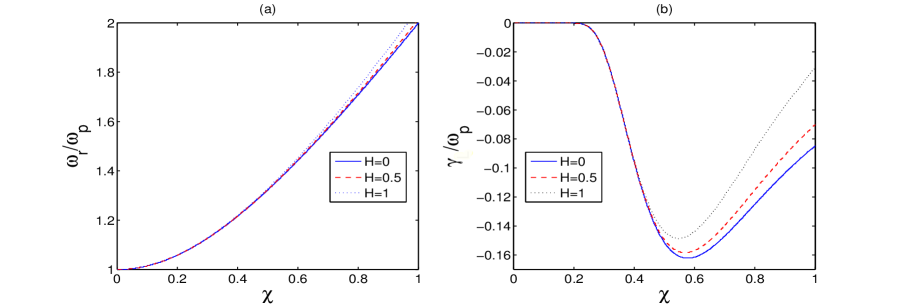
Figure 4: The wave dispersion [panel (a)] and the damping rate [panel (b)] are shown (reproduced from Ref. chatterjee2016 ) against $\chi\equiv k\lambda_{D}$ for different values of $H$ as in the legends.

Case-II: We consider a fully degenerate plasma, i.e., a zero-temperature Fermi gas with the following background distribution of electrons.

$$f_{0}(\mathbf{v})=\left\{\begin{array}[]{cc}{2m^{3}}/{(2\pi\hbar)^{3}},&|\mathbf{v}|\leq v_{F}\\ 0,&|\mathbf{v}|>v_{F},\end{array}\right.$$ (33)

where $v_{F}=\sqrt{2E_{F}/m}$ is the electron Fermi velocity and $E_{F}=\hbar^{2}\left(3\pi^{2}n_{0}\right)^{2/3}/2m$ is the Fermi energy. Performing the velocity integral on the $v_{y}v_{z}$ plane, i.e., perpendicular to the $v_{x}$-axis and using the cylindrical coordinates in $v_{y}$ and $v_{z}$, we obtain (replacing $v_{x}$ by $v$)

$$F_{0}(v)=\left\{\begin{array}[]{cc}\left[{2\pi m^{3}}/{(2\pi\hbar)^{3}}\right](v_{F}^{2}-v^{2}),&|{v}|\leq v_{F}\\ 0,&\rm{otherwise}.\end{array}\right.$$ (34)

We note that the distribution function (33), which is flat topped in three dimensions, becomes parabolic in one dimension. So, there is a possibility that the resonant velocity $v^{\rm{res}}_{\pm}$ falls in the negative slope of the distribution function $F_{0}(v)$ for which the wave damping occurs. In order to assess it we must require an expression for the dispersion relation. The dispersion equation (25) after evaluating the principal value integral using Eq. (34) reduces to eliasson2010 ; misra2017

$$1+\frac{3\omega_{p}^{2}}{4k^{2}v_{F}^{2}}\left(2-\sum_{j=\pm 1}\frac{j}{2v_{q}v_{F}}\left\{v_{F}^{2}-\left(v_{p}+jv_{q}\right)^{2}\right\}\log\left|\frac{v_{p}+jv_{q}-v_{F}}{v_{p}+jv_{q}+v_{F}}\right|\right)=0.$$ (35)

Equation (35) can be analyzed numerically to ascertain whether the resonant velocity $v^{\rm{res}}_{\pm}$ remains smaller than $v_{F}$ in some domain of $k\lambda_{F}$ for which the Landau damping can occur. Here, $\lambda_{F}=v_{F}/\omega_{p}$ is the Fermi wavelength, $v^{\rm{res}}_{\pm}/v_{F}=v_{p}/v_{F}\pm Hk\lambda_{F}/2$ and $H=\hbar\omega_{p}/mv_{F}^{2}$ (in degenerate plasmas $v_{t}$ is to be replaced by $v_{F}$). In order that the quantum effects to be important and the Langmuir wavelength is not much larger than the de Broglie wavelength, we must have $\hbar k/mv_{F}\equiv k\lambda_{B}=Hk\lambda_{F}\lesssim 1$, i.e., $k\lambda_{F}<1/H$. The smaller values of $H~{}(\lesssim 1)$ corresponds to high density regimes. From the analysis of the dispersion relation (35) as in Ref. misra2017 it can be moted that there is a small regime of the Langmuir wavelength $0<k\lambda_{F}\lesssim 1$ for which $v^{\rm{res}}_{\pm}<v_{F}$ is satisfied. For example, when $H\sim 1$, the relation $v^{\rm{res}}_{-}<v_{F}$ holds for $0.9\lesssim k\lambda_{F}\lesssim 1$. As the values of $H$ decrease from $H=1$, the resonant velocities shift towards higher values of $k\lambda_{F}>1$. So, the Landau damping due to the one-plasmon resonance may occur for $k\lambda_{F}>1$ and $H\lesssim 1$. Consequently, such damping does not occur in the regime of $H<1$ with $0\lesssim k\lambda_{F}<1$ misra2017 , and so is in the semi-classical limit $\hbar k/mv_{F}\ll 1$. In the latter, the dispersion equation (35) reduces to

$$1+\frac{3\omega_{p}^{2}}{2k^{2}v_{F}^{2}}\left(1-\frac{v_{p}}{v_{F}}\log\left|\frac{v_{p}+v_{F}}{v_{p}-v_{F}}\right|\right)=0.$$ (36)

The term ‘semi-classical’ is used because, the dispersion relation (36) can also be derived from the one-dimensional Vlasov-Poisson equation using the background distribution of electrons given by Eq. (33). Since for $H<1$ and in the regime $0\lesssim k\lambda_{F}<1$, the Landau damping does not occur, the logarithmic functions in Eq. (35) can be expanded for small wave numbers. Thus, retaining the terms involving $k$ up to $k^{4}$, one obtains eliasson2010

$$\omega^{2}=\omega_{p}^{2}+\frac{3}{5}k^{2}v_{F}^{2}+(1+\alpha)\frac{\hbar^{2}k^{4}}{4m^{2}},$$ (37)

where $\alpha=(48/175)m^{2}v_{F}^{4}/\hbar^{2}\omega_{p}^{2}$ is a correction term which becomes smaller than unity in low-density plasmas, e.g., metals and semiconductors. However, it can be larger than unity in highly dense environments. A term similar to $\alpha$ was also obtained and discussed by Ferrell in his work on the characteristics of electron plasma oscillations in metals ferrell1957 .

It is to be noted that a critical value $k_{\rm{cr}}$ of the wave number $k$ and hence the corresponding critical wave frequency $\omega_{\rm{cr}}$ exist such that the Landau damping occurs for $k>k_{\rm{cr}}$ and $\omega>\omega_{\rm{cr}}$. The critical values can be obtained from the resonance condition $v=\omega/k-\hbar k/2m\leq v_{F}$, i.e.,

$$\omega_{\rm{cr}}\equiv k_{\rm{cr}}v_{F}+\hbar k_{\rm{cr}}^{2}/2m,$$ (38)

and the following reduced equation for $k_{\text{cr}}$ [after substituting $\omega=\omega_{\rm{cr}}$ in Eq. (35)] eliasson2010

$$1+\frac{3\omega_{p}^{2}}{4k_{\rm{cr}}^{2}v_{F}^{2}}\left[2-\left(2+\frac{\hbar k_{\rm{cr}}}{mv_{F}}\right)\log\left(1+\frac{2mv_{F}}{\hbar k_{\rm{cr}}}\right)\right]=0.$$ (39)

An approximate expression for the Landau damping rate can be obtained by using the formalism $\gamma/\omega_{r}=-(1/2)D_{i}(\omega_{r},k)$ and noting that $v_{F}^{3}=3\pi^{2}n_{0}\hbar^{3}/m^{3}$ as

$$\frac{\gamma}{\omega_{r}}=-\frac{3\pi}{4}\frac{\omega_{r}\omega_{p}^{2}}{k^{3}v_{F}^{3}}.$$ (40)

It follows that the Landau damping rate $|\gamma|$ gets reduced at higher values of $k$. The regions for the existence of damped and undamped waves are discussed in Ref. eliasson2010 .

Case-III: Following the work of Melrose and Mushtaq melrose2010 , we consider the background distribution of electrons as a three-dimensional Fermi gas with arbitrary degeneracy. In this case, the linear dielectric function will be the same as Eq. (24), however, the three-dimensional background distribution of electrons is given by

$$f_{0}(v)\equiv 2\bar{n}(v)\left(\frac{m}{2\pi\hbar}\right)^{3}=2\left(\frac{m}{2\pi\hbar}\right)^{3}\left[1+\exp\left(\frac{\varepsilon-\mu_{0}}{k_{B}T}\right)\right]^{-1},$$ (41)

where $\bar{n}(v)$ is the occupation number of electrons, $\varepsilon=(m/2)(v_{x}^{2}+v_{y}^{2}+v_{z}^{2})$ is the kinetic energy and $\mu_{0}$ is the equilibrium chemical potential related to the equilibrium number density $n_{0}$ which satisfies the following charge neutrality condition.

$$n_{0}=\int f_{0}(v)d^{3}v.$$ (42)

The parameter $\mu_{0}/k_{B}T$ determines the level of degeneracy of electrons. It can take from large negative values to large positive values as one enters the regions from nondegenerate to fully degenerate plasmas. Thus, $\xi_{0}\equiv\exp(\mu_{0}/k_{B}T)\ll 1$ in the nondegenerate limit $T\gg T_{F}$ for which one can recover the Maxwellian distribution and $\xi_{0}\gg 1$ in the fully degenerate limit $(T\ll T_{F})$. The case with $T\gtrsim T_{F}$ such that $\xi_{0}~{}(<0)$ is of moderate value, corresponds to a partially degenerate plasma. Noting that $d^{3}v=v^{2}\sin\theta dvd\theta d\phi$ with $0<v<\infty$, $0\leq\theta\leq\pi$ and $0\leq\phi\leq 2\pi$, and integrating over $\theta$ and $\phi$, we obtain from Eq. (24) the following expression for the electron susceptibility $[D(\omega,k)\equiv 1-\chi(\omega,k)]$ melrose2010

$$\chi(\omega,k)=\frac{4\pi e^{2}m}{\varepsilon_{0}(2\pi\hbar)^{3}}\frac{1}{2k\Delta}\int d\varepsilon\bar{n}(\varepsilon)\left[\log\Big{|}\frac{\omega-a\sqrt{\varepsilon}+\Delta}{\omega+a\sqrt{\varepsilon}+\Delta}\Big{|}-\log\Big{|}\frac{\omega-a\sqrt{\varepsilon}-\Delta}{\omega+a\sqrt{\varepsilon}-\Delta}\Big{|}\right],$$ (43)

where $\Delta=kv_{q}$ and $a=\sqrt{(2/m)}k$.

Equation (42) is rewritten as

$$n_{0}=\frac{2m^{3}}{(2\pi\hbar)^{3}}\sqrt{\frac{2}{m}}\frac{4\pi}{m}\int^{\infty}_{0}\sqrt{\varepsilon}\bar{n}(\varepsilon)d\varepsilon.$$ (44)

Next, using in it the distribution function (41) and noting that

$$Li_{\nu}(-z)=-\frac{1}{\Gamma(\nu)}\int_{0}^{\infty}\frac{s^{\nu-1}}{1+z^{-1}e^{s}}ds,~{}\nu>0;~{}~{}Li_{\nu}(z)=\sum_{n=1}^{\infty}\frac{z^{n}}{n^{\nu}},~{}|z|<1,$$ (45)

we obtain

$$n_{0}=-\frac{2(2\pi)^{3/2}m^{3}v_{t}^{3}}{(2\pi\hbar)^{3}}Li_{3/2}(-\xi_{0}),$$ (46)

or, using the expression for the Fermi temperature $k_{B}T_{F}=(\hbar^{2}/2m)(3\pi^{2}n_{0})^{2/3}$, we write

$$-Li_{3/2}(-\xi_{0})=\frac{4}{3\sqrt{\pi}}\left(\frac{T_{F}}{T}\right)^{3/2},$$ (47)

Such an expression of $T_{F}$ can also be obtained from Eq. (46) in the limit of $\xi_{0}\gg 1$ so that $\mu_{0}\approx k_{B}T_{F}$ and $Li_{\nu}(-\xi_{0})\approx-(\mu_{0}/k_{B}T)^{\nu}/\Gamma(\nu+1)$. The expression for $n_{0}$ [Eq. (46)] is applicable for arbitrary degeneracy of electrons, and using it one can obtain the total number density as

$$n=n_{0}\frac{Li_{3/2}(-\xi)}{Li_{3/2}(-\xi_{0})},$$ (48)

where $\xi=\exp(\mu/k_{B}T)$.

A power series expansion in $\xi_{0}$ of the expression of $\bar{n}$, i.e., $\bar{n}(\varepsilon)=\left[1+\xi_{0}^{-1}\exp(\varepsilon/k_{B}T)\right]^{-1}$ can be made in the limit of $\xi_{0}\ll 1$ to give

$$\bar{n}(\varepsilon)=\sum_{s=1}^{\infty}(-1)^{s-1}\xi_{0}^{s}\exp(-s\varepsilon/k_{B}T).$$ (49)

The expression for $\bar{n}(\varepsilon)$ [Eq. (49)] can be inserted in Eq. (43) to yield

$$D(\omega,k)=1-\frac{2\pi^{3/2}e^{2}m^{2}v_{t}^{2}}{\varepsilon_{0}(2\pi\hbar)^{3}k\Delta}\sum_{s=1}^{\infty}(-1)^{s-1}\frac{\xi_{0}^{s}}{s}\left[Z\left(\sqrt{\frac{s}{k_{B}T}}y_{+}\right)-Z\left(\sqrt{\frac{s}{k_{B}T}}y_{-}\right)\right],$$ (50)

where $y_{\pm}=(\omega\pm\Delta)/a$ and $Z$ is the plasma dispersion function, given by,

$$Z(\zeta)=\frac{1}{\sqrt{\pi}}\int_{-\infty}^{\infty}\frac{e^{-t^{2}}}{t-\zeta}dt.$$ (51)

Since the plasma dispersion function can have real and imaginary parts, and also $\zeta$ can be large or small, three cases may be of interest: the case where the Landau resonance contributes; the high- $(Y_{\pm}\equiv y_{\pm}/\sqrt{k_{B}T}=(\omega\pm\Delta)/\sqrt{2}kv_{t}\gg 1)$ and low-frequency $(Y_{\pm}\ll 1)$ limits according to when $\zeta$ is large or small. The low-frequency limit is disregarded to this study as we will simplify the dispersion relation for high-frequency Langmuir waves and associated Landau damping.

In the limit of $Y_{\pm}\gg 1$, only the real part of $Z(\zeta)$, where

$$Z(\zeta)=i\sqrt{\pi}e^{-\zeta^{2}}-\zeta^{-1}\left[1+(1/2\zeta^{2})+(3/4\zeta^{4})+\cdots\right],~{}|\zeta|\gg 1,$$ (52)

is of particular interest. So, one obtains

$$Z\left(\sqrt{\frac{s}{k_{B}T}}y_{+}\right)-Z\left(\sqrt{\frac{s}{k_{B}T}}y_{-}\right)=\sqrt{\frac{2}{s}}\frac{2\Delta kv_{t}}{\omega^{2}-\Delta^{2}}\left[1+\frac{k^{2}v_{t}^{2}}{s}\frac{3\omega^{2}+\Delta^{2}}{(\omega^{2}-\Delta^{2})^{2}}+\cdots\right].$$ (53)

Thus, using the expression (53), Eq. (50) reduces to

$$D(\omega,k)=1-\frac{\omega_{p}^{2}}{\omega^{2}-\Delta^{2}}-\omega_{p}^{2}k^{2}v_{t}^{2}\frac{3\omega^{2}+\Delta^{2}}{(\omega^{2}-\Delta^{2})^{3}}G,$$ (54)

where $G=Li_{5/2}(-\xi_{0})/Li_{3/2}(-\xi_{0})\approx\sqrt{1+(T_{F}/5T)^{2}}$ in which an interpolation has been made by assuming that $G\rightarrow 1$ for $T\gg T_{F}$ (non-degenerate limit) and $G\rightarrow v_{F}^{2}/5v_{t}^{2}$ for $T\ll T_{F}$ (completely degenerate limit). Although, Eq. (54) is obtained using the power series expansion of $\bar{n}(\varepsilon)$ in the limit of $\xi_{0}\ll 1$, an alternative derivation [for details see Eq. (9) of melrose2010 ] suggests that the dielectric function (54) is applicable for arbitrary degeneracy of electrons. Thus, from Eq. (54), we obtain the following dispersion relation for Langmuir waves in plasmas with arbitrary degeneracy.

$$\omega^{2}=\omega_{p}^{2}+\Delta^{2}+\omega_{p}^{2}k^{2}v_{t}^{2}\frac{3\omega^{2}+\Delta^{2}}{(\omega^{2}-\Delta^{2})^{2}}G.$$ (55)

In absence of any thermal flow, we have $\omega^{2}=\omega_{p}^{2}+\Delta^{2}$. So, if the thermal correction is small, this expression of $\omega^{2}$ can be substituted in Eq. (55) to yield

$$\omega^{2}=\omega_{p}^{2}+3k^{2}v_{t}^{2}G+\frac{\hbar^{2}k^{4}}{4m^{2}},$$ (56)

where we have retained the terms involving $k$ up to ${\cal O}(k^{4})$. In the nondegenerate limit $G\rightarrow 1$, Eq. (56) reduces to the known dispersion relation for Langmuir waves [cf. Eq. (30)], i.e.,

$$\omega^{2}=\omega_{p}^{2}+3k^{2}v_{t}^{2}+\frac{\hbar^{2}k^{4}}{4m^{2}}.$$ (57)

On the other hand, in the fully degenerate limit, i.e., $G\rightarrow v_{F}^{2}/5v_{t}^{2}$, Eq. (56) gives

$$\omega^{2}=\omega_{p}^{2}+(3/5)k^{2}v_{F}^{2}+\frac{\hbar^{2}k^{4}}{4m^{2}},$$ (58)

which agrees with Eq. (37) obtained before except an additional factor $(1+\alpha)$ to the term $\propto k^{4}$. Such a disagreement may be due to an approximation made in the derivation of Eq. (54) in the nondegenerate limit $\xi_{0}\ll 1$. Melrose and Mushtaq melrose2010 made an interpolation formula between the nondegenerate and fully degenerate limits to obtain the following dispersion relation for Langmuir waves with arbitrary degeneracy.

$$\omega^{2}=\omega_{p}^{2}+3k^{2}\left[v_{t}^{4}+\left(\frac{v_{F}^{2}}{5}\right)^{2}\right]^{1/2}+\frac{\hbar^{2}k^{4}}{4m^{2}}.$$ (59)

From Eq. (50), the imaginary part can be obtained as

$$\Im D(\omega,k)=\sqrt{\frac{\pi}{2}}\frac{\omega_{p}^{2}}{kv_{t}}\frac{1}{2\Delta}\left[Li_{1}\left(-\xi_{0}e^{-Y_{-}^{2}}\right)-Li_{1}\left(-\xi_{0}e^{-Y_{+}^{2}}\right)\right]\Big{/}Li_{3/2}(-\xi_{0}),$$ (60)

which, after using the relation $Li_{1}(z)=\sum_{n=1}^{\infty}z^{n}/n=-\log(1-z)$, reduces to

$$\Im D(\omega,k)=\sqrt{\frac{\pi}{2}}\frac{\omega_{p}^{2}}{kv_{t}}\frac{1}{2\Delta}\frac{1}{Li_{3/2}(-\xi_{0})}\log\left(\frac{1+\xi_{0}e^{-Y_{+}^{2}}}{1+\xi_{0}e^{-Y_{-}^{2}}}\right).$$ (61)

Thus, for arbitrary degeneracy, the Landau damping rate of Langmuir waves can be obtained by using either $\gamma/\omega_{r}=-(1/2)D_{i}(\omega_{r},k)$ or $\gamma=-{D_{i}(\omega_{r},k)}/\left(\partial D_{r}/\partial\omega_{r}\right)$ and noting that $\partial D_{r}/\partial\omega_{r}\approx 2\omega_{p}^{2}/\omega_{r}^{3}$ for small $k$, i.e.,

$$\gamma=-\sqrt{\frac{\pi}{2}}\frac{\omega_{r}^{3}}{kv_{t}}\frac{1}{4\Delta}\frac{1}{Li_{3/2}(-\xi_{0})}\log\left(\frac{1+\xi_{0}e^{-Y_{+}^{2}}}{1+\xi_{0}e^{-Y_{-}^{2}}}\right).$$ (62)

From Eq. (62) it can be assessed that the Landau damping in degenerate plasmas becomes smaller than that in non-degenerate plasmas. An alternative derivation of the dielectric function for Langmuir waves in one-dimensional geometry in arbitrary degenerate plasmas can be found in Ref. rightley2016 .

Case-IV: So far we have studied the dispersion properties and the Landau damping rates of high-frequency Langmuir waves as described in Cases I to III. Here, we study those for low-frequency electron-acoustic waves (EAWs) in a partially degenerate plasma with two-temperature (low with the suffix ‘$l$’ and high with the suffix ‘$h$’) electrons and stationary ions. Such partially degenerate plasmas, where the background distribution of electrons deviate from thermodynamic equilibrium, can appear in the context of laser produced plasmas or ion-beam driven plasmas hau-riege2011 ; gibbon2005 . Similar to the previous cases, our starting point is the Wigner-Moyal and the Poisson system [Eqs. (19) and (20)] which are rewritten for $\alpha$-species electrons as

$$\begin{split}\frac{\partial f_{\alpha}}{\partial t}+{\bf v}\cdot\nabla_{\bf r}f_{\alpha}+\frac{iem^{3}}{(2\pi)^{3}\hbar^{4}}\int\int d^{3}{\bf r}^{\prime}d^{3}{\bf v}^{\prime}e^{im({\bf v}-{\bf v}^{\prime})\cdot{\bf r}^{\prime}/\hbar}&\left[\phi\left({\bf r}+\frac{{\bf r}^{\prime}}{2},t\right)-\phi\left({\bf r}-\frac{{\bf r}^{\prime}}{2},t\right)\right]\\ &\times f_{\alpha}({\bf r},{\bf v}^{\prime},t)=0,\end{split}$$ (63)

and the Poisson equation

$$\nabla^{2}\phi=\frac{e}{\varepsilon_{0}}\left(\sum_{\alpha=l,h}\int f_{\alpha}d^{3}v-n_{0}\right),$$ (64)

where $n_{0}$ is the unperturbed number density of stationary ions. For the one-dimensional propagation of EAWs along the $x$-axis, the background distribution function for electrons is the projected Fermi-Dirac distribution (writing $v_{x}$ as $v$).

$$\begin{split}f_{\alpha}^{(0)}(v)&=\int\int f^{3D}_{\alpha}({\bf v})dv_{y}dv_{z}\\ &=2\left(\frac{m}{2\pi\hbar}\right)^{3}\int\int\left[1+\exp\left(\frac{\varepsilon-\mu_{\alpha}}{k_{B}T_{\alpha}}\right)\right]^{-1}dv_{y}dv_{z}\\ &=\frac{3}{4}\frac{n_{\alpha 0}}{v_{F\alpha}}\frac{T_{\alpha}}{T_{F\alpha}}\log\left[1+\exp\left(-\frac{\frac{1}{2}mv^{2}-\mu_{\alpha}}{k_{B}T_{\alpha}}\right)\right],\end{split}$$ (65)

where $\mu_{\alpha}$ is the equilibrium chemical potential which satisfies the following charge neutrality condition.

$$n_{0}=\sum_{\alpha}\int f_{\alpha}^{(0)}(v)dv.$$ (66)

As said before, in the nondegenerate limit $(T_{\alpha}\gg T_{F\alpha})$, the parameter $\xi_{\alpha}=\mu_{\alpha}/k_{B}T_{\alpha}$ is large and negative, while it is large and positive in the fully degenerate limit $(T_{\alpha}\ll T_{F\alpha})$. We, however, consider the case of $T_{\alpha}\gtrsim T_{F\alpha}$ such that $\xi_{\alpha}~{}(<0)$ is of moderate value. Here, we note that there are certain parameter restrictions imposed by the Pauli’s exclusion principle as we cannot have a phase space density of the background Wigner function exceeding $2(m/2\pi\hbar)^{3}$. As a result, the parameters for the high- and low-temperature electron distributions cannot be chosen independently. The strictest criterion appears for $\varepsilon=0$ leading to

$$\left[{1+\exp\left(-\frac{\mu_{l}}{k_{B}T_{l}}\right)}\right]^{-1}+\left[{1+\exp\left(-\frac{\mu_{h}}{k_{B}T_{h}}\right)}\right]^{-1}\leq 1.$$ (67)

For a partially degenerate low-temperature distribution (i.e., $k_{B}T_{l}\sim E_{F}$, $\mu_{l}\sim 2E_{F}$), this condition is typically fulfilled if the high-temperature distribution is not too far from the classical Maxwell-Boltzmann regime such that $-\mu_{h}/k_{B}T_{h}\gtrsim 3$.

Fourier analyzing Eqs. (63) and (64) by considering $f_{\alpha}(x,v,t)=f_{\alpha}^{(0)}+f_{\alpha}^{(1)}$ and $\phi(x,t)=\phi^{(1)}$, and assuming the perturbations to be of the form $\sim\exp(ikx-i\omega t)$, we obtain the following dispersion relation.

$$D(\omega,k)\equiv 1-\sum_{\alpha=l,h}\frac{\omega_{p\alpha}^{2}}{n_{\alpha_{0}}k^{2}}\int_{-\infty}^{\infty}\frac{f_{\alpha}^{(0)}(v)}{(v-\omega/k)^{2}-{v_{q}^{2}}}dv=0,$$ (68)

where $\omega_{p\alpha}=\sqrt{n_{\alpha 0}e^{2}/\varepsilon_{0}m}$ is the plasma frequency for $\alpha$-species electrons. Assuming the wave damping to be small with $\omega=\omega_{r}+i\gamma$, we obtain from $D(\omega,k)\equiv D_{r}(\omega_{r},k)+iD_{i}(\omega_{r},k)+i\gamma[\partial D_{r}(\omega_{r},k)/\partial\omega_{r}]=0$ the dielectric function

$$D_{r}(\omega_{r},k)\equiv 1-\sum_{\alpha=l,h}\frac{\omega_{p\alpha}^{2}}{n_{\alpha 0}k^{2}}{\cal P}\int\frac{f_{\alpha}^{(0)}(v)}{(v-\omega_{r}/k)^{2}-v_{q}^{2}}dv=0,$$ (69)

and the Landau damping rate

$$\gamma=-\frac{D_{i}(\omega_{r},k)}{\partial D_{r}/\partial\omega_{r}},$$ (70)

where

$$D_{i}=-2\pi v_{q}\sum_{\alpha=l,h}\frac{\omega_{p\alpha}^{2}}{n_{\alpha 0}k^{2}}\left[f_{\alpha}^{(0)}(v^{\text{res}}_{+})-f_{\alpha}^{(0)}(v^{\text{res}}_{-})\right],$$ (71)

in which $v^{\text{res}}_{\pm}=\omega_{r}/k\pm v_{q}$ denotes the plasmon resonance velocity.

Next, substituting the distribution function (65) into Eq. (69) and evaluating the integrals in two different regimes $|v|<\omega_{r}/k\pm v_{q}$ and $|v|>\omega_{r}/k\pm v_{q}$, i.e.,

$$\begin{split}{\cal P}\int_{-\infty}^{\infty}&=\lim_{\epsilon\rightarrow 0+}\left[\int_{-\infty}^{-(\lambda\pm v_{q})}+\int_{-(\lambda\pm v_{q})}^{(\lambda\pm v_{q})-\epsilon}+\int_{(\lambda\pm v_{q})+\epsilon}^{\infty}\right]\\ &=\lim_{\epsilon\rightarrow 0+}\left[\int_{-(\lambda\pm v_{q})}^{(\lambda\pm v_{q})-\epsilon}+2\int_{(\lambda\pm v_{q})+\epsilon}^{\infty}\right],\end{split}$$ (72)

and noting that the exponential function in the distribution function [Eq. (65)] is small in the partially degenerate regime, we obtain misra2021

$$D_{r}(\omega_{r},k)\equiv 1-\frac{3}{4}\sum_{\alpha=l,h}\omega_{p\alpha}^{2}e^{\xi_{\alpha}}\left[2\sqrt{2}\frac{v_{t\alpha}/v_{F\alpha}}{\omega_{r}^{2}-k^{2}v_{q}^{2}}+\frac{\sqrt{2\pi}v_{t\alpha}-\omega_{r}/k}{k^{2}v_{t\alpha}^{2}v_{F\alpha}}\right]=0.$$ (73)

Equation (73) describes both the high-frequency and relatively low-frequency branches of electrostatic waves. In the limit of $\omega_{r}/k\pm v_{q}\gg v_{th}$, the high-frequency Langmuir wave (LW) mode can be obtained from Eq. (73) by considering the first and the second terms as

$$\omega_{r}^{2}=k^{2}v_{q}^{2}+\frac{3}{\sqrt{2}}\sum_{\alpha=l,h}\omega_{p\alpha}^{2}\frac{v_{t\alpha}}{v_{F\alpha}}e^{\xi_{\alpha}},$$ (74)

where $v_{t\alpha}=\sqrt{2k_{B}T_{\alpha}/m}$ is the thermal velocity and $v_{F\alpha}=\sqrt{2k_{B}T_{F\alpha}/m}$ the Fermi velocity of $\alpha$-species electrons. On the other hand, for $\omega_{r}/k\pm v_{q}\ll v_{tl}$, the first and the third terms of Eq. (73) can be combined to yield the following dispersion relation for the EAW mode.

$$\omega_{r}=k\left(\sqrt{2\pi}\sum_{\alpha=l,h}\frac{\omega_{p\alpha}^{2}e^{\xi\alpha}}{v_{t\alpha}v_{F\alpha}}-\frac{4}{3}k^{2}\right)\Big{/}\sum_{\alpha=l,h}\frac{\omega_{p\alpha}^{2}e^{\xi\alpha}}{v^{2}_{t\alpha}v_{F\alpha}}.$$ (75)

Furthermore, Eq. (66) for the equilibrium chemical potentials reduces to

$$\frac{3}{4}\sqrt{\pi}\sum_{\alpha=l,h}\left(\frac{T_{\alpha}}{T_{F\alpha}}\right)^{3/2}n_{\alpha 0}e^{\xi_{\alpha}}=n_{0}.$$ (76)

Since the dispersion relations (74) and (75) are obtained by assuming the smallness of the exponential function in the distribution function (65), the classical results of LWs and EAWs cannot be recovered directly from Eqs. (74) and (75). The reason is that the Fermi-Dirac distribution approaches the Maxwell-Boltzmann distribution in the limit of low density or high temperature, i.e., when the integrand in Eq. (65) is much smaller than the unity.

From Eq. (75) we note that the EAW has the properties similar to the ion-acoustic waves in an electron-ion plasma. For typical plasma parameters $n_{l0}=2\times 10^{24}$ cm^-3, $n_{h0}=10-12n_{l0}$, $T_{l}=10^{6}$ K and $T_{h}=2.5-3T_{l}$, and with $kv_{th}/\omega_{ph}\equiv k\lambda_{h}\ll 1$, Eq. (75) reduces to $\omega_{r}\approx 2.5kv_{th}$. This predicts the phase velocity of EAWs a bit higher than predicted in the classical theory holloway1991 $(\omega_{r}\approx 1.31kv_{th})$. The profiles of the dispersion curves and the Landau damping rates are shown in Fig. 5. It is found that depending on the values of the ratios $T=T_{l}/T_{h}$ or $N=n_{l0}/n_{h0}$, a critical value $K_{c}$ of $K\equiv k\lambda_{h}$ exists, beyond which the EAW frequency can turn over, going to zero, and then assume negative values. Such a distinctive nature of the wave frequency does not appear in classical plasmas where the high- and low-frequency branches form a thumb-like curve holloway1991 and it may be due to the finite temperature degeneracy of background electrons. A considerable regime of $K$ where the Landau damping rate of EAWs remains weak is found to be $0\lesssim K\lesssim 0.5$ or $\hbar k/mv_{th}\lesssim 0.2$.

!

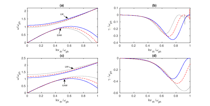
Figure 5: The profiles of the dispersion curves of Langmuir waves (LWs) and electron-acoustic waves (EAWs) [Subplots (a) and (c)], given by Eqs. (74) and (75), and the Landau damping rates for EAWs [Subplots (b) and (d)], given by Eq. (70), are shown. The figure is reproduced from Ref. misra2021 . For subplots (a) and (b), the fixed parameters are $n_{l0}=2\times 10^{24}$ cm^-3, $T_{l}=10^{6}$ K and $T_{h}=2.5T_{l}$; the solid, dashed and dotted lines, respectively, correspond to $n_{h0}=10n_{l0}$, $11n_{l0}$ and $12n_{l0}$. For subplots (c) and (d), the fixed parameters are $n_{l0}=2\times 10^{24}$ cm^-3, $n_{h0}=10n_{l0}$ and $T_{l}=10^{6}$ K; the solid, dashed and dotted lines, respectively, correspond to $T_{h}=2.5T_{l}$, $2.7T_{l}$ and $3T_{l}$.

2.3 Landau damping in relativistic quantum plasmas

In high-enrgy density plasmas, especially in the laser-based inertial fusion plasma experiments and laser-based plasma compression schemes, electrons become highly relativistic due to laser-driven ponderomotive force. So, it is required to consider a relativistic quantum kinetic model for the description of wave-particle interactions in high-energy density plasmas. A theoretical study along this line was made by Zhu and Ji zhu2012 . According to their work, we consider the relativistic quantum kinetic model which is established by the covariant Wigner function and Dirac equation. The covariant form of one-particle Wigner function is defined as

$$f^{\mu}(x,p)=\frac{1}{(2\pi\hbar)^{4}}\int d^{4}y\exp(-ip^{\mu}y_{\mu}/\hbar)\Big{\langle}\bar{\psi}\left(x+\frac{1}{2}y\right)\gamma^{\mu}\psi\left(x-\frac{1}{2}y\right)\Big{\rangle}.$$ (77)

Here, $p$ is the relativistic particle momentum, $\gamma^{\mu}$ with $\mu=0,1,2,3$ are the matrices which can be expressed in terms of $2\times 2$ sub-matrices of the Pauli matrices and the $2\times 2$ identity matrix, and are such that $\{\gamma^{\mu},\gamma^{\nu}\}=2\eta^{\mu\nu}I_{4}$, where $\eta$ is the Minkowski metric with metric signature $(+---)$, $I_{4}$ is the $4\times 4$ identity matrix, and the bracketed expression $\{a,b\}=ab+ba$ denotes the anti-commutator. The angular brackets $\langle...\rangle$ in Eq. (77) denote a quantum statistical average, i.e., $\langle...\rangle=\rm{Tr}\{...\rho\}$ with $\rho$ denoting the density operator that characterizes the statistical state of the system and $\psi$ (with $\bar{\psi}$ denoting its conjugate) the wave function satisfying the following Dirac equation.

$$\left[\gamma^{\mu}\left(i\hbar\partial_{\mu}+\frac{e}{c}A_{\mu}(x)\right)-mc\right]\psi(x)=0,$$ (78)

where $A_{\mu}=(-\phi,cA)$ is the Minkowski four-vector operator of the electromagnetic potential which satisfies the D’Alembert’s equation in covariant form

$$\square\langle A^{\mu}(x)\rangle=-\frac{e}{\varepsilon_{0}mc}\int d^{4}pp^{\mu}f(x,p).$$ (79)

Here, $\square\equiv\partial^{\mu}\partial_{\mu}$ is the D’Alembert operator and $f(x,p)$ is defined by

$$f(x,p)=\frac{1}{(2\pi\hbar)^{4}}\int d^{4}y\exp(-ip^{\mu}y_{\mu}/\hbar)\Big{\langle}\bar{\psi}\left(x+\frac{1}{2}y\right)\psi\left(x-\frac{1}{2}y\right)\Big{\rangle}.$$ (80)

Next, the evolution equation for $f^{\mu}(x,p)$ can be obtained by taking the derivative of Eq. (77) and using the Dirac equation (78) as

$$\begin{split}\partial_{\mu}f^{\mu}(x,p)+\frac{ie}{\hbar c}\frac{1}{(2\pi\hbar)^{4}}\int\int d^{4}yd^{4}p^{\prime}\exp\left[-i(p-p^{\prime})\cdot y/\hbar\right]&\left[A_{\mu}\left(x+\frac{1}{2}y\right)-A_{\mu}\left(x-\frac{1}{2}y\right)\right]\\ &\times f^{\mu}(x,p^{\prime})=0,\end{split}$$ (81)

where $p\cdot y=p^{\mu}y_{\mu}$. The Dirac current operator $\bar{\psi}\left(x+{y}/{2}\right)\gamma^{\mu}\psi\left(x-{y}/{2}\right)$ can be decomposed into a convective part and the current due to the spin and magnetic moment of particles. In the weakly relativistic limit, the spin and magnetic moment contributions can be neglected. So, under this approximation one obtains from Eq. (77) using the Lorenz gauge condition, i.e., $\partial_{\mu}A^{\mu}(x)=0$ as (See for details Ref. zhu2012 )

$$f^{\mu}(x,p)\approx\frac{1}{mc}\left(p^{\mu}+\frac{e}{c}A^{\mu}(x)\right)f(x,p),$$ (82)

and Eqs. (79) and (81) reduce to

$$\square\langle A^{\mu}(x)\rangle=-\frac{e}{\varepsilon_{0}mc}\int d^{4}pp^{\mu}f(x,p)-\frac{4\pi e^{2}}{mc^{2}}\langle A^{\mu}(x)\rangle\int d^{4}pf(x,p),$$ (83)

$$\begin{split}&\left(p^{\mu}+\frac{e}{c}A^{\mu}(x)\right)\partial_{\mu}f^{\mu}(x,p)-\frac{ie}{\hbar c}\frac{1}{(2\pi\hbar)^{4}}\int\int d^{4}yd^{4}p^{\prime}\exp\left[-i(p-p^{\prime})\cdot y/\hbar\right]\\ &\times\left[A_{\mu}\left(x+\frac{1}{2}y\right)-A_{\mu}\left(x-\frac{1}{2}y\right)\right]\left(p^{\mu}+\frac{e}{c}A^{\mu}(x)\right)f^{\mu}(x,p^{\prime})=0.\end{split}$$ (84)

Next, Fourier analyzing Eqs. (83) and (84) by assuming $f(x,p)=f_{0}(p)+f_{1}(x,p)$ and $\langle A^{\mu}(x)\rangle=O+A_{1}^{\mu}(x)$, and using the Lorenz gauge condition $k_{\mu}A_{1}^{\mu}(k)=0$, we obtain the following dispersion relation.

$$\rm{Det}\left[\left(\Omega_{p}^{2}/c^{2}-k_{\nu}k^{\nu}\right)\eta^{\mu\sigma}+\omega_{p}^{2}K^{\mu\sigma}/c^{2}\right]=0,$$ (85)

where $\Omega_{p}^{2}=(\omega_{p}^{2}/n_{0})\int d^{4}pf_{0}(p)$ is the relativistic quantum plasma frequency and $K^{\mu\sigma}$ is the dielectric permittivity tensor, given by,

$$K^{\mu\sigma}=\frac{1}{\hbar n_{0}}\int d^{4}p\frac{p^{\mu}p^{\sigma}}{k_{\nu}p^{\nu}}\left[f_{0}\left(p+\frac{1}{2}\hbar k\right)-f_{0}\left(p-\frac{1}{2}\hbar k\right)\right].$$ (86)

In a frame where the equilibrium four-velocity component is $(1,0,0,0)$ and the wave propagates along the third-axis, Eq. (85) reduces to

$$\left(\Omega_{p}^{2}-c^{2}k_{\mu}k^{\mu}-\omega_{p}^{2}K^{11}\right)^{2}\left[\left(\Omega_{p}^{2}-c^{2}k_{\mu}k^{\mu}+\omega_{p}^{2}K^{00}\right)\left(\Omega_{p}^{2}-c^{2}k_{\mu}k^{\mu}-\omega_{p}^{2}K^{33}\right)+\omega_{p}^{4}K^{30}/c^{2}\right]=0.$$ (87)

The first factor of Eq. (87) gives the transverse mode

$$\omega_{T}^{2}=\Omega_{p}^{2}+c^{2}k^{2}-\omega_{p}^{2}K^{11}.$$ (88)

On the other hand, the second factor of Eq. (87) after using the current conservation equation $k_{\mu}\Pi^{\mu\nu}(k)=0$, where $\Pi^{\mu\nu}$ is the polarization tensor, i.e., $\Pi^{\mu\nu}(k)=-\left(\omega_{p}^{2}K^{\mu\nu}+\Omega_{p}^{2}\eta^{\mu\nu}\right)/4\pi$, gives the following longitudinal mode.

$$\omega_{L}^{2}=\Omega_{p}^{2}+c^{2}k^{2}+\omega_{p}^{2}K^{00}-\frac{\omega}{kc}\omega_{p}^{2}K^{30}.$$ (89)

In a fully degenerate plasma the background distribution of electrons can be considered as

$$f_{0}(p)=\frac{2mc^{3}}{(2\pi\hbar)^{3}}\int d^{4}p^{\prime}\delta(p-p^{\prime})2\theta(p^{\prime}_{0}c)\delta(p^{\prime 2}c^{2}-m^{2}c^{4})\theta(\varepsilon_{F}-p_{0}^{\prime}c),$$ (90)

where $\delta$ is the Dirac delta function, $\theta$ is the Heaviside step function, $\varepsilon_{F}$ is the electron Fermi energy and $p_{0}^{\prime}$ is the classical momentum.

Substituting the distribution function [Eq. (90)] into Eq. (86) and assuming that $\hbar\omega\ll E_{p}\equiv(m^{2}c^{4}+p^{2}c^{2})^{1/2}$, $\hbar k\ll p$ and $v_{F}\ll v_{\text{ph}}$, we obtain reduced expressions for $K^{00}$, $K^{30}$, and $K^{11}$. Using these expressions of $K$’s and considering the weakly relativistic limit $(p_{F}\ll mc)$, we obtain from Eq. (89)

$$\omega_{L}^{2}=\omega_{p}^{2}\left(1-\frac{1}{2}\beta_{F}^{2}\right)+\frac{3}{5}k^{2}v_{F}^{2}\left(1-\frac{3}{2}\beta_{F}^{2}\right)+\frac{\hbar^{2}k^{4}}{4m^{2}}\left(1-\frac{3}{2}\beta_{F}^{2}\right),~{}~{}(v_{F}\ll v_{\text{ph}})$$ (91)

where $\beta_{F}=v_{F}/c$. Similarly, one can obtain the dispersion relation for electromagnetic wave in a weakly relativistic quantum plasma as

$$\omega_{T}^{2}=\omega_{p}^{2}\left(1-\frac{1}{2}\beta_{F}^{2}\right)+c^{2}k^{2}+\frac{\hbar^{2}k^{4}}{4m^{2}}\left(1-\frac{3}{2}\beta_{F}^{2}\right).$$ (92)

In the limit of $\beta_{F}\rightarrow 0$, Eq. (91) reduces to the dispersion relation of Langmuir waves in a nonrelativistic fully degenerate plasma as discussed in Case II. Also, in the classical limit $\hbar\rightarrow 0$ together with the limit $\beta_{F}\rightarrow 0$, we recover from Eq. (92) the classical dispersion relation of electromagnetic waves. Note that since in the weakly relativistic approximation, the phase velocity of electromagnetic waves is much higher than the Fermi velocity, the possibility of Landau damping is ruled out. So, we are interested only with the Langmuir waves. An expression for the Landau damping rate can be obtained by using $\gamma/\omega_{r}=-(1/2)D_{i}(\omega_{r},k)$ as zhu2012

$$\frac{\gamma}{\omega_{r}}=-\frac{3\pi}{4}\frac{\omega_{p}^{2}\omega_{r}}{k^{3}v_{F}^{3}}\left(1+\beta_{F}^{2}+\frac{1}{8}\frac{\hbar^{2}k^{2}}{m^{2}c^{2}}\right),~{}~{}(v_{F}>v_{\text{ph}}),$$ (93)

where $\omega_{r}\equiv\omega_{L}$.

A comparison of the dispersion properties and associated Landau damping of Langmuir waves can be made in classical plasmas, nonrelativistic quantum plasmas and relativistic quantum plasmas. Comparing the Landau damping rates for Langmuir waves in classical and fully degenerate plasmas we find that

$$\frac{\gamma_{\mathrm{cl}}}{\gamma_{\mathrm{F}}}\sim\pi\sqrt{2\pi}e^{-3/2}n_{0}\lambda_{B}^{3}\sim 1.8n_{0}\lambda_{B}^{3}.$$ (94)

Equation (94) shows that since for quantum plasmas $n_{0}\lambda_{B}^{3}\geq 1$, the Landau damping rate in classical plasmas is higher than that in fully degenerate plasmas. On the other hand, the ratio of the damping rates in non-relativistic and relativistic quantum plasmas gives

$$\frac{\gamma_{\mathrm{rq}}}{\gamma_{\mathrm{nq}}}\sim 1+\beta_{F}^{2}+\frac{1}{8}\frac{\hbar^{2}k^{2}}{m^{2}c^{2}}.$$ (95)

It follows from Eq. (95) that the Landau damping rate in relativistic regime is a bit higher than that in nonrelativistic regime due to the relativistic factor $\beta_{F}$ and the quantum recoil associated with the particle dispersion $\propto\hbar^{2}$. Similarly, the classical Landau damping rate can also be shown to be higher than that in non-relativistic quamtum plasmas with finite temperature degeneracy. The reason is that for degenerate plasmas, most of the electron energy levels are filled up to the Fermi energy and number of free electrons to take part in the resonance is reduced. As a result, the energy conversion between Langmuir waves and degenerate particles are not so effective as in classical plasmas. The dispersion relations and the Landau damping rates so obtained in different plasmas with various background distributions are summarized in Table 1. It is noted that depending on the quantum effect weak or strong, the background distribution changes from Boltzmann to Fermi-Dirac statistics.

System	Background distribution	Dispersion relation	Landau damping rate
Classical plasma	Maxwellian	$\omega^{2}=\omega_{p}^{2}+3k^{2}v_{t}^{2}$	$\frac{\gamma}{\omega}=-\sqrt{\frac{\pi}{8}}\frac{\omega_{p}^{2}\omega}{k^{3}v_{t}^{3}}$ $\times\exp\left(-\frac{\omega^{2}}{2k^{2}v_{t}^{2}}\right)$
Non-relativistic quantum plasma	Maxwellian	$\omega^{2}=\omega_{p}^{2}+3k^{2}v_{t}^{2}$ $+\frac{\hbar^{2}k^{4}}{4m^{2}}$	$\frac{\gamma}{\omega}=-\sqrt{\frac{\pi}{8}}\frac{\omega_{p}^{2}\omega}{k^{3}v_{t}^{3}}\left[1-\frac{1}{6}\frac{v_{q}^{2}}{v_{t}^{2}}\left(3-\frac{\omega^{2}}{k^{2}v_{t}^{2}}\right)\right]$ $\times\exp\left(-\frac{\omega^{2}}{2k^{2}v_{t}^{2}}\right)$
Non-relativistic quantum plasma	Fermi-Dirac (Zero temperature)	$\omega^{2}=\omega_{p}^{2}+\frac{3}{5}k^{2}v_{F}^{2}$ $+(1+\alpha)\frac{\hbar^{2}k^{4}}{4m^{2}}$	$\frac{\gamma}{\omega}=-\frac{3\pi}{4}\frac{\omega\omega_{p}^{2}}{k^{3}v_{F}^{3}}$
Non-relativistic quantum plasma	Fermi-Dirac (Finite temperature)	$\omega^{2}=\omega_{p}^{2}+3k^{2}$ $\times\left[v_{t}^{4}+(v_{F}^{2}/5)^{2}\right]^{1/2}$ $+\frac{\hbar^{2}k^{4}}{4m^{2}}$	$\frac{\gamma}{\omega}=-\sqrt{\frac{\pi}{2}}\frac{\omega^{2}}{kv_{t}}\frac{(1/4\Delta)}{Li_{3/2}(-\xi)}$ $\times\log\left(\frac{1+\xi e^{-Y_{+}^{2}}}{1+\xi e^{-Y_{-}^{2}}}\right)$
Relativistic quantum plasma	Fermi-Dirac (Zero temperature)	$\omega^{2}=\omega_{p}^{2}\left(1-\frac{1}{2}\beta_{F}^{2}\right)$ $+\frac{3}{5}k^{2}v_{F}^{2}\left(1-\frac{3}{2}\beta_{F}^{2}\right)$ $+\frac{\hbar^{2}k^{4}}{4m^{2}}\left(1-\frac{3}{2}\beta_{F}^{2}\right)$	$\frac{\gamma}{\omega}=-\frac{3\pi}{4}\frac{\omega\omega_{p}^{2}}{k^{3}v_{F}^{3}}$ $\times\left(1+\beta_{F}^{2}+\frac{1}{8}\frac{\hbar^{2}k^{2}}{m^{2}c^{2}}\right)$

Table 1: Dispersion relations and Landau damping rates derived in classical, non-relativistic quantum plasmas, and relativistic quantum plasmas.

3 Wave-particle interactions: Nonlinear theory

So far we have discussed the linear theory of wave-particle interactions, especially the Landau damping in classical and quantum regimes. We have seen that while the linearized Vlasov-Poisson system in classical and weak quantum (semiclassical) regimes gives the phase velocity resonance, the linearized Wigner-Moyal equation predicts the wave damping where the particle’s resonant velocity is shifted from the phase velocity by a velocity $v_{q}=\hbar k/2m$ due to quantum effects. Going beyond the linear theory, we will see that while the phase velocity or group velocity is still the resonant velocity in the classical or weak quantum regime, in the strong quantum regime there appear some additional resonances with velocity shifts $nv_{q}$, $n=2,3,...$, called multi-plasmon resonances which can occur due to simultaneous absorption (or emission) of multiple plasmon quanta brodin2017 .

On the other hand, it is known from the classical theory that for a homogeneous plasma wave, i.e., a wave with infinite extent rather than a localized pulse, the linear Landau damping can turn into nonlinear bounce oscillations with the bounce frequency of trapped particles $\omega_{B}=(ek^{2}\Phi/m)^{1/2}$ oneil1965 ; nicholson1983 , where $\Phi$ is the potential amplitude of the wave field. However, in quantum plasmas not only the modification of such classical behaviors occurs but also a complete suppression of the linear Landau resonance can be seen depending on which regime (weak or strong quantum) we consider. Our aim in Sec. 3.1 is to demonstrate these phenomena, especially to show the existence of bounce-like oscillations even in absence of trapped particles in the weak quantum regime and the emergence of nonlinear multi-plasmon resonance in the strong quantum regime. Although, many of the more well-known aspects of Landau damping can be studied for an infinite plane wave, there are still some rooms to generalize this setup to the more realistic case of localized waves and wave packets where the phase velocity or group velocity resonances enter the picture in the weak quantum regime together with the nonlinear multi-plasmon resonances in the strong quantum regime. We will also consider these nonlinear resonant wave-particle interactions in Secs. 3.2 to 3.5 on the assumption that the particle trapping time by the wave, i.e., $\tilde{\omega}^{-1}_{B}$ is typically longer than the time by which the wave gets damped, i.e., $\gamma>\tilde{\omega}_{B}$, where $\gamma$ is the linear Landau damping rate.

3.1 Wave-particle interactions in the nonlinear homogeneous regime

For a homogeneous plasma, particles to be trapped and the nonlinearities to be important, the bounce frequency must fulfill $\omega_{B}$ $>\gamma$. As noted, the classical behaviors can be modified in the quantum regime; so, we consider two regimes, namely the weak quantum and the strong quantum regimes. Firstly, for the case of weak damping, when the linear resonance is located in the tail of the distribution, quantum effects can influence the dynamics in a regime that is seemingly classical. In particular, even if the conditions for the classical regime, $v_{F}\ll v_{t}$ and $\hbar k/mv_{t}\ll 1$, are both fulfilled, the nonlinear regime of wave-particle interaction may still be strongly modified by quantum effects. This phenomenon will be considered in the first subsection 3.1.1 below. Secondly, we will consider a completely degenerate system, and focus on the strong quantum regime, in which case $\hbar k/mv_{F}\sim 1$. Here, we will be concerned with the case where linear wave-particle damping is suppressed completely, but where nonlinear wave-particle interaction is possible due to processes involving simultaneous absorption of multiple wave-quanta.

3.1.1 The weak quantum regime

In this subsection, we consider a nearly classical case with $v_{F}\ll v_{t}$ and $\hbar k/mv_{t}\ll 1$, and a resonance in the tail of the background electron distribution. Due to the weak quantum condition, the linear resonant velocity will be close to the phase velocity. To assure that the damping is modest, i.e. $\gamma/\omega$ $\ll 1$, we will assume that $\omega/kv_{t}<1$ with some margin. After an initial simplification, using the above inequalities, the dynamical equation is solved numerically as in Ref. brodin2015 . The key steps in simplifying the full Wigner-Poisson system are as follows:

1. Due to the resonance being located in the tail of the distribution, the nonlinearity sets in for a modest amplitude. Specifically, we have $ek\Phi/m\omega v_{t}\ll 1$. Together with the condition $\hbar k/mv_{t}\ll 1$, this means the linear Vlasov equation applies for most of the velocity space, except close to the resonance, where the full equation (nonlinear Wigner equation) must be solved.

2. The resonance region is defined by $[v_{\mathrm{res}}-\delta v_{\mathrm{res}},v_{\mathrm{res}}+\delta v_{\mathrm{res}}]$, and defines the region where the full nonlinear Wigner equation is solved (as opposed to the linearized Vlasov equation). As long as $\delta v_{\mathrm{res}}$ fulfills $\hbar k/2m\ll\delta v_{\mathrm{res}}\ll kv_{t}^{2}/\omega\,$, the results are insensitive to the exact width of the resonance region $\delta v_{\mathrm{res}}.$

3. In the resonance region, the ansatz for the one-dimensional Wigner function is a general periodic function, i.e., it can be written in the form

   $$g=g_{0}(\mathbf{v})+\delta g_{0}(\mathbf{v,}t)+\left[\sum_{n=1}^{\infty}g_{n}(\mathbf{v,}t)\exp i[n(kz-\omega t)]+\mathrm{c.c}\right].$$ (96)

4. In a practical calculation scheme, the sum over harmonics needs to be truncated. The number of harmonics to be required will vary, mainly depending on the combined quantum and nonlinearity parameter  $e\Phi/\hbar\omega_{B}=m\omega_{B}/\hbar k^{2}$.

Based on the points 1 to 4, Ref. brodin2015 reduced the Wigner-Poisson equations to the following normalized equations.

$$\frac{\partial\hat{\Phi}(t)}{\partial t}=\frac{1}{\pi}\int_{\mathrm{res}}g_{1}dv,$$ (97)

$$\frac{\partial g_{1}}{\partial t}+ivg_{1} = \hat{\Phi}\left[1+\frac{g_{0}(v+\delta v_{q})-g_{0}(v-\delta v_{q})}{2\delta v_{q}}\right]+\hat{\Phi}^{\ast}\left[\frac{g_{2}(v+\delta v_{q})-g_{2}(v-\delta v_{q})}{2\delta v_{q}}\right],$$ (98)

$$\frac{\partial g_{n}}{\partial t}+invg_{n} = \hat{\Phi}\left[\frac{g_{n-1}^{\ast}(v+\delta v_{q})-g_{n-1}^{\ast}(v-\delta v_{q})}{2\delta v_{q}}\right]+\hat{\Phi}^{\ast}\left[\frac{g_{n+1}(v+\delta v_{q})-g_{n+1}(v-\delta v_{q})}{2\delta v_{q}}\right],$$ (99)

and

$$\frac{\partial g_{0}}{\partial t}=\hat{\Phi}\left[\frac{g_{1}^{\ast}(v+\delta v_{q})-g_{1}^{\ast}(v-\delta v_{q})}{2\delta v_{q}}\right]+\hat{\Phi}^{\ast}\left[\frac{g_{1}(v+\delta v_{q})-g_{1}(v-\delta v_{q})}{2\delta v_{q}}\right],$$ (100)

where $n\geq 2$ in Eq. (99). The physical quantities are normalized according to: the time $t\rightarrow\gamma t$, the velocity $v_{z}\rightarrow kv_{z}/\gamma$, the potential $\Phi\rightarrow ek^{2}\Phi/\gamma^{2}m$ and the normalized harmonics of the Wigner function is $(kg_{n}/\gamma)\left[\partial G_{0}(v_{z})/\partial v_{z}\right]_{\omega/k}$. Finally, the quantum velocity shift, occurring in the arguments of $g_{n}$, is given by $\delta v_{q}=hk^{2}/2m\gamma$.

An advantage with the above system of Eqs. (97)–(100), as compared to the initial system, is that the time-steps larger than the inverse plasma frequency can be used. Moreover, the equations only need to be solved in a small part of velocity space, close to the resonance. Finally, the spatial dependence is solved for analytically in Eqs. (97)–(100), which further simplifies the numerics. A detailed numerical study of Eqs. (97)–(100) was presented in Ref. brodin2015 . Here, we will only present the main features, which were the following:

1. A quantum modification of the nonlinear bounce frequency. Specifically, the classical nonlinear bounce frequency $\omega_{B}$ is replaced by a quantum correspondence $\tilde{\omega}_{B}$ with a lower value given by $\tilde{\omega}_{B}=\omega_{B}/(1+\hbar k^{2}/2m\gamma)$. Thus, when $\hbar k^{2}/2m\gamma\gg 1$ is fulfilled, there is a substantial difference in the bounce frequency. Due to the smallness of the linear damping, the decrease in the bounce frequency can be appreciable even in the regime $\hbar k/mv_{t}\ll 1$.

2. Quantum suppression of the nonlinear bounce oscillations. Classically, for $\omega_{B}>\gamma$, we have nonlinear bounce oscillations. However, the corresponding quantum condition is $\tilde{\omega}_{B}>\gamma$. Thus, in the regime where $\tilde{\omega}_{B}<\gamma<\omega_{B}$, classical theory will be thoroughly invalidated as the nonlinear oscillations will be completely suppressed, and instead linear damping takes place. Apart from Ref. brodin2015 , this feature was also observed in Ref. daligault2014 , using a slightly different approach.

3. Bounce-like oscillations in the absence of trapped particles. Classically nonlinear oscillations take place due to particles being trapped in the potential well of the plasma oscillations. In the regime where $\omega_{B}>\hbar k^{2}/2m$, however, the connection between nonlinear oscillations and trapped particles completely disappears. In this regime, there are no trapped particles, since the lowest energy state of the potential well will be higher than the trapping potential. However, the nonlinear bounce-like oscillations can still take place. In this case, the energy oscillates between different harmonics of the perturbed distribution function leading to bounce-like oscillations of the electrostatic potential.

The above features taken together show that the quantum behaviors can be seen in a regime that on the surface is classical as we have used $\hbar k/mv_{t}\ll 1$ and $v_{F}\ll v_{t}$. The main reason making this possible is that the characteristic scale length in velocity space is very short for the case of a resonance in the tail of the electron distribution. As a result, the sharp localization in velocity space triggers a large quantum uncertainty in physical space, and hence the system will be subject to quantum modifications of the classical theory. While the above results refer to quantum modifications when the resonance is located in the tail of the distribution, we note that some of the above features also remain when the resonance lies close to the bulk of the distribution although the plasma temperature and density must fit into the typical quantum regime in that case. Specifically, numerical results presented in Ref. suh1991 show that the quantum suppression of nonlinear behaviors can be applicable also in that case.

3.1.2 The strong quantum regime

In the strong quantum regime, we have short wavelengths $\hbar k\sim mv_{F}$ and a high plasma density, i.e., $H\sim 1$. Typically, there is no regime resembling the classical bounce oscillations in that case. However, an interesting effect occurs in the degenerate regime, when the resonance of Eq. (25) occurs at a velocity slightly larger than the Fermi velocity. In that case, the linear wave-particle damping may be absent and be replaced by a nonlinear counterpart. To understand how this may happen, let us take a first look at the linear wave-particle resonance. As noticed in Eq. (25), the quantum mechanical adjustment of the resonant velocity is given by

$$v^{\text{res}}=\frac{\omega}{k}\rightarrow v^{\text{res}}=\frac{\omega}{k}\pm\frac{\hbar k}{2m}.$$ (101)

Let us study the physical meaning of this result briefly. When a particle absorbs or emits a wave quantum it can increase or decrease the momentum according to

$$\hbar k_{1}\pm\hbar k=\hbar k_{2},$$ (102)

and at the same time the energy changes according to

$$\hbar\omega_{1}\pm\hbar\omega=\hbar\omega_{2}.$$ (103)

Next, we identify $\hbar k_{1}/m$ (or equally well $\hbar k_{2}/m$) with the resonant velocity $v^{\text{res}}$ and note that for small amplitude waves, the frequencies and wave numbers $(\omega_{1,2},k_{1,2})$ obey the free particle dispersion relation $\omega_{1,2}=\hbar k_{1,2}^{2}/2m$. Using these relations, we can deduce that the energy momentum relations [Eqs. (102) and (103)] imply the modification of the resonant velocity as seen in Eq. (101). An interesting possibility, which was studied in Ref. brodin2017 , is the simultaneous absorption (or emission) of multiple wave quanta rather than a single wave quantum at a time. In that case, Eqs. (102) and (103) are replaced by

$$\hbar k_{1}\pm n\hbar k=\hbar k_{2},$$ (104)

and

$$\hbar\omega_{1}\pm n\hbar\omega=\hbar\omega_{2},$$ (105)

where $n=1,2,3,\ldots$ is an integer. Accordingly, performing the same algebra as for the linear case, the resonant velocities now become

$$v_{\pm n}^{\text{res}}=\frac{\omega}{k}\pm n\frac{\hbar k}{2m}.$$ (106)

When we pick the minus sign in Eq. (106), the resonant velocity for absorbing multiple wave quanta can be considerably low provided the wavelengths are short. As a consequence, in the case of Langmuir waves, the damping rate due to absorption of multiple wave quanta can be much larger than the standard linear damping rate. This is due to the larger number of resonant particles in the former case.

While the physical conditions are slightly different, mathematically things are very similar to the weak quantum case as we need to solve the Vlasov-Poisson system. Importantly, in the weakly nonlinear regime, wave-particle interaction due to multi-plasmon damping is a slow process such that a perturbative approach can be applied. Moreover, the division of velocity space into a resonance and a nonresonance regions is still possible. As a result, the system of equations resembles that of the previous section (Sec. 3.1.1). Specifically, the simplified Wigner equation, after weakly nonlinear approximations have been made, can be written as

$$\begin{split}\partial_{t}f_{0}&=-\frac{ie}{\hbar}(\Phi_{1}\operatorname{\overset{\leftrightarrow}{D}}_{1}f_{1}^{\ast}-\Phi_{1}^{\ast}\operatorname{\overset{\leftrightarrow}{D}}_{1}f_{1}+\Phi_{2}\operatorname{\overset{\leftrightarrow}{D}}_{2}f_{2}^{\ast}-\Phi_{2}^{\ast}\operatorname{\overset{\leftrightarrow}{D}}_{2}f_{2}),\\ \partial_{t}{f_{1}}-i(\omega-kv_{z})f_{1}&=-\frac{ie}{\hbar}(\Phi_{1}\operatorname{\overset{\leftrightarrow}{D}}_{1}(F_{0}+f_{0})-\Phi_{1}^{\ast}\operatorname{\overset{\leftrightarrow}{D}}_{1}f_{2}+\Phi_{2}\operatorname{\overset{\leftrightarrow}{D}}_{2}f_{1}^{\ast}-\Phi_{2}^{\ast}\operatorname{\overset{\leftrightarrow}{D}}_{2}f_{3}),\\ \partial_{t}f_{n}-in(\omega-kv_{z})f_{n}&=-\frac{ie}{\hbar}(\Phi_{1}\operatorname{\overset{\leftrightarrow}{D}}_{1}f_{n-1}-\Phi_{1}^{\ast}\operatorname{\overset{\leftrightarrow}{D}}_{1}f_{n+1}+\Phi_{2}\operatorname{\overset{\leftrightarrow}{D}}_{2}f_{n-2}^{\ast}-\Phi_{2}^{\ast}\operatorname{\overset{\leftrightarrow}{D}}_{2}f_{n+2}),\quad(n>1),\end{split}$$ (107)

where $f_{n}$ denotes the harmonics of the Wigner-function. Moreover, we use the same quantum velocity shift $\mathbf{v}_{q}$ as before and we have introduced a velocity shift operator $\operatorname{\overset{\leftrightarrow}{D}}_{n}$, defined by,

$$(\operatorname{\overset{\leftrightarrow}{D}}_{n}f)(\mathbf{v})=f(\mathbf{v}+n\mathbf{v}_{q})-f(\mathbf{v}-n\mathbf{v}_{q}).$$ (108)

While the governing equations resemble Eqs. (98)–(100), an important difference is that the harmonics of the electrostatic potential must be included in the treatment. Moreover, before solving the equations, further simplifications need to be done, which is slightly different depending on whether the main damping is due to the resonance for $n=2$ (two-plasmon resonance) or for $n=3$ (three plasmon resonance) (see Ref. brodin2017 for details). Finally, the equations are solved numerically. Interestingly, the results for two-plasmon damping and three-plasmon damping are similar. In both the cases, since the damping mechanism is nonlinear, the damping rate decays with the amplitude. Importantly, the numerical results for the damping rate can be fitted to the following expression.

$$|\Phi(t)|=|\Phi(0)|/(1+t/t_{0})^{1/2},$$ (109)

where $t_{0}$ is a characteristic damping time that scales as

$$t_{0}\sim C(v_{q},\omega/k)\left|\frac{\hbar\omega}{e\Phi(0)}\right|^{2}\frac{1}{\omega}.$$ (110)

From the numerical results, it is found that the dimensionless coefficient $C$ varies in between $0.03-0.5$ as a function of the velocity shift and the phase velocity (see Ref. brodin2017 for details). While the magnitudes of the two-plasmon and the three-plamon damping rates are of comparable magnitude, generally the damping due to the three-plasmon processes occurs slightly faster. This follows from the fact that the resonance occurs somewhat deeper into the bulk of the background electron distribution for the three-plasmon resonance.

While the effect of multi-plasmon damping is most pronounced for a completely degenerate system as the competing linear processes may vanish completely, it can also be prominent at a finite temperature as discussed in some detail in Ref. brodin2017 . Moreover, as should be clear from the discussion leading up to Eq. (106) that the damping mechanism is of a very general nature. In principle, in case the wavelength is short enough to make quantum effects important, the same type of multi-quanta damping mechanism applies to all types of wave-modes not just the plasmons.

3.2 Nonlinear Landau damping of ion-acoustic solitary waves in the weak quantum regime

While the nonlinear wave-particle interaction in homogeneous plasmas is of basic theoretical interest, in a practical context, wave-particle interaction typically competes with other nonlinear processes. In particular, it is well known that the nonlinear propagation of small amplitude ion-acoustic waves (IAWs) in a plasma with warm electrons and cold ions is asymptotically governed by the Korteweg-de Vries (KdV) equation. The significant modification of this equation due to electron Landau damping was noted and studied by Ott and Sudan ott1969 on the assumption that particle’s trapping time is much longer than that of Landau damping. The theory was later advanced by Vandam and Taniuti vandam1973 to take into account the ion Landau resonance under the consideration that the Landau damping is a far-field approximation of the Vlasov equation, i.e., a small amplitude long-wavelength wave will damp after a long time. The theory of Landau damping of IAWs was, however, further studied in the context of plasmas in the semiclassical or weak quantum regime by Barman and Misra barman2017 . According to their work, we consider the nonlinear propagation of ion-acoustic waves (IAWs) and the wave-particle interaction in an unmagnetized collisionless plasma with weak quantum effects, i.e., when the typical ion-acoustic length scale is larger than the thermal de Broglie wavelength. In order to include the resonance effects both from quantum electrons and classical ions we consider the semi-classical Vlasov equation for electrons, Vlasov equation for ions and the Poisson equation, given by,

$$\frac{\partial f_{e}}{\partial t}+v\frac{\partial f_{e}}{\partial x}+\frac{1}{m_{0}}\frac{\partial\phi}{\partial x}\frac{\partial f_{e}}{\partial v}-\frac{H^{2}}{24m_{0}^{2}}\frac{\partial^{3}\phi}{\partial x^{3}}\frac{\partial^{3}f_{e}}{\partial v^{3}}=0,$$ (111)

$$\frac{\partial f_{i}}{\partial t}+v\frac{\partial f_{i}}{\partial x}-\frac{\partial\phi}{\partial x}\frac{\partial f_{i}}{\partial v}=0,$$ (112)

$${\frac{\partial^{2}\phi}{\partial x^{2}}}=-\sum_{j=e,i}\theta_{j}\int f_{j}dv,$$ (113)

In Eqs. (111) to (113) we have normalized the physical quantities according to $v\rightarrow v/c_{s}$, $\phi\rightarrow e\phi/k_{B}T_{e}$, $n_{j}\rightarrow n_{j}/n_{0}$, and $f_{j}\rightarrow f_{j}c_{s}/n_{0}$ where $c_{s}=\sqrt{k_{B}T_{e}/m_{i}}\equiv\omega_{pi}\lambda_{D}$ is the IAW speed with $\omega_{pi}=\sqrt{n_{0}e^{2}/\varepsilon_{0}m_{i}}$ denoting the ion plasma frequency. Also, $n_{0}$ is the equilibrium number density of electrons and ions, and $T_{j}$ is the thermodynamic temperature of electrons $(j=e)$ and ions $(j=i)$. The space and time variables are normalized by $\lambda_{D}$ and $\omega^{-1}_{pi}$ respectively. Furthermore, $m_{0}=m/m_{i}$ is the electron to ion mass ratio, $H=\hbar\omega_{p}/k_{B}T_{e}$ is the dimensionless quantum parameter denoting the ratio of the electron plasmon energy to the thermal energy and $\theta_{j}=\mp 1$ for $j=e~{}(i)$.

An evolution equation for the small amplitude IAWs can be derived following Refs. vandam1973 ; barman2017 , i.e., using the multi-scale asymptotic expansion technique in which $\phi$ and $f_{j}$ are expanded in different powers of $\epsilon$, where $\epsilon~{}(\lesssim 1)$ is a small positive scaling parameter measuring the weakness of perturbations. In the weak quantum regime, the background distribution of electrons and ions [i.e., $f^{(0)}_{j}$, for $j=e,i$] can be assumed to be the Maxwellian. Furthermore, different expansions for $f_{j}$ are to be considered in the non-resonance $\left(|v-\omega/k|\gg o(\epsilon)\right)$ and resonance $(v\approx\omega/k)$ regions. Also, in order to properly include the contributions of resonant particles, the multi-scale Fourier-Laplace transforms for $f_{j}-f^{(0)}_{j}$ and $\phi$ are to be employed. A standard perturbation scheme with the stretched coordinates $\xi=\epsilon^{1/2}x,~{}\sigma=\epsilon^{1/2}t,~{}s=\epsilon^{3/2}x$ yields the following evolution equation for the first order potential perturbation of IAWs (for details see Ref. barman2017 ).

$$\frac{\partial\phi}{\partial s}+\alpha\phi\frac{\partial\phi}{\partial\zeta}+\beta\frac{\partial^{3}\phi}{\partial\zeta^{3}}+\gamma~{}\text{P}\int_{-\infty}^{\infty}(\zeta-\zeta^{\prime})^{-1}\frac{\partial\phi(\zeta^{\prime})}{\partial\zeta^{\prime}}d\zeta^{\prime}=0,$$ (114)

where $\zeta=\xi-v_{p}\sigma$ and the coefficients are given by $\alpha=b/a$, $\beta=1/a$ and $\gamma=c/a$ in which $a$, $b$ and $c$ are simplified to

$$a=2v_{p}^{-2}\left(1+6v_{p}^{-2}T^{-1}\right)+v_{p}H^{2}k,$$ (115)

$$b=3v_{p}^{-4}+30T^{-1}v_{p}^{-6}-1,$$ (116)

$$c=\epsilon^{-1}\frac{v_{p}}{\sqrt{2\pi}}\left[m_{0}^{1/2}+T^{3/2}\exp\left(-\frac{Tv_{p}^{2}}{2}\right)\right].$$ (117)

Here, $T=T_{e}/T_{i}$ with $T_{i}$ denoting the ion temperature and the term $\propto\gamma$ appears due to the wave-particle resonance and $v_{p}$ is the nonlinear wave phase speed $\lambda\equiv\omega/k$, given by,

$$v_{p}^{2}=\frac{1+\sqrt{1+(12/T)\left(1+{H^{2}k^{2}}/{12}\right)}}{2\left(1+{H^{2}k^{2}}/{12}\right)}.$$ (118)

It is noted that the dispersion relation is modified by the quantum correction $\propto H$. In the limit of $T\gg 1$ and $H^{2}k^{2}/12\ll 1$, Eq. (118) reduces to

$$v_{p}\approx 1+\frac{3}{2T}-\frac{H^{2}k^{2}}{24}.$$ (119)

It follows that in contrast to the quantum fluid theory haas2003 or classical kinetic theory vandam1973 , the phase velocity $v_{p}$ is no longer a constant, i.e., the wave becomes dispersive due to the quantum effects. A careful analysis shows that the wave speed $v_{p}$ always decays with the wave number $k$. However, it can be increased or decreased depending on the values of $H$ and $T$. The linear damping rate $\gamma$ [Fig. 6] is also seen to decrease with increasing values of $k$ and $H$. However, a critical value of $T\sim 24$ exists below (above) which the value of $\gamma$ decreases (increases) with an increasing value of $T$.

It is pertinent to mention that in the derivation of the KdV equation (114), not only the Landau damping (linear resonance) contributes to the wave dynamics, there also appears a term involving the effects of particle trapping (nonlinear resonance). However, we have disregarded such term as the results with the trapping effects are similar to the classical theory vandam1973 . So, we study mainly the linear Landau damping effect on the ion-acoustic solitary waves. We also note that each of the coefficients $a,~{}b$ and $c$ are modified by the quantum parameter $H$, in absence of which one recovers the classical results of Vandam et al. vandam1973 .

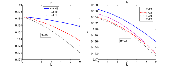
Figure 6: The Landau damping rate $\gamma$ (normalized by $\omega_{pi}$) is plotted against the wave number $k$ (normalized by $\lambda_{D}^{-1}$) in three different cases: (a) when $T$ is fixed and $H$ varies, (b) when $H$ is fixed and $T$ varies and (c) when the value of $T$ is relatively lower than that in the plots (a) and (b). The figure is reproduced from Ref. barman2017 .

In order to study the effects of the linear Landau damping on the profile of ion-acoustic solitary waves we find an approximate solitary wave solution of Eq. (114) on the assumption that the effect of the Landau damping ($\varpropto\gamma$) is small, i.e., $\gamma\ll\alpha~{}(\gtrsim\beta)$, which holds when $T\gtrsim 20$ and $H<1$, as barman2014

$$\phi=\Psi~{}\text{sech}^{2}\left[\left(\zeta-\frac{\alpha}{3}\int_{0}^{s}\Phi ds\right)/W\right]+o(\gamma),$$ (120)

where $\Psi=\Phi_{0}\left(1+{s}/{s_{0}}\right)^{-2}$ is the amplitude of the solitary wave solution of the KdV equation (114), and $\Phi=3U_{0}/\alpha$ is the corresponding amplitude, $W=\left({12\beta}/{\Phi\alpha}\right)^{1/2}\equiv\sqrt{4\beta/U_{0}}$ is the width and $U_{0}=\Phi\alpha/3$ is the constant phase speed (normalized by $c_{s}$) of the solitary wave solution of the KdV equation in absence of the Landau damping (i.e., when $\gamma$ or $c=0$). Also, $\Phi=\Phi_{0}$ at $s=0$ and $s_{0}$ is given by

$$s_{0}^{-1}=\frac{\gamma}{4}\sqrt{\frac{\alpha\Phi_{0}}{3\beta}}\text{P}\int_{-\infty}^{\infty}\int_{-\infty}^{\infty}\frac{\text{sech}^{2}z}{z-z^{\prime}}\frac{\partial}{\partial z^{\prime}}\left(\text{sech}^{2}z^{\prime}\right)dzdz^{\prime}.$$ (121)

It is found that the wave amplitude decays with time and the decay rate is relatively low (compared to the classical result ott1969 ) in the weak quantum regime.

Some estimates for the bounce freuencies of electrons and ions, as well as a comparison of the contributions from the linear and nonlinear resonances on the wave damping can be made. If $\omega_{B}=\sqrt{e\phi/m}/W$ denotes the bouncing frequency, the electron trapping time by a solitary pulse is $\sim\omega_{B}^{-1}$. Since for small amplitude perturbations, the wave potential scales as $\phi\sim\epsilon$, we have $\omega_{B}\sim\omega_{p}\sqrt{\epsilon}\sim\omega_{pi}\epsilon^{-1/2}$ for $\epsilon\sim\sqrt{m/m_{i}}$. However, from Fig. 6 it can be estimated that the Landau damping rate, $\gamma\sim 0.18\omega_{pi}$ for some values of $T,~{}H$ and $k$. So, the condition $\gamma<\omega_{B}$ holds for electrons be trapped. On the other hand, since for ions $\omega_{B}\sim\omega_{pi}\sqrt{\epsilon}$, one has $\gamma>\omega_{B}$ and ion trapping may be neglected. For the nonlinear resonance we find vandam1973

$$\int_{res.}f_{j}dv\approx-\frac{v_{p}}{\sqrt{2\pi}}\left[\exp\left(-\frac{1}{2}m_{0}v_{p}^{2}\right)+\epsilon T^{3/2}\exp\left(-\frac{1}{2}Tv_{p}^{2}\right)\right].$$ (122)

Thus, from Eqs. (117) and (122), it is clear that the effects of the linear resonance is relatively higher than that of the nonlinear one (trapping). Nevertheless, ions may be reflected by a solitary pulse and propagate as a precursor tiwari2016 .

Some important points are to be mentioned. In the semiclassical regime since $T_{e}>T_{F}$ holds, the Pauli blocking is reduced and the particles’ collisions can influence the dynamics of IAWs. However, the inclusion of a collisional term in the semiclassical Vlasov equation is not so straightforward. If a small collisional effect (e.g., Coulomb collision) is introduced, the effective electron-electron collision frequency scales as $\nu_{ef}\sim\epsilon\omega_{p}\left(n_{0}\lambda_{D}^{3}\right)^{-1}\sim\epsilon^{-2}\omega_{pi}\left(n_{0}\lambda_{D}^{3}\right)^{-1}$. For moderate density plasmas with $n_{0}\sim 6\times 10^{23}$ cm^-3 and $T_{e}\sim 7\times 10^{6}$ K, one can have $\left(n_{0}\lambda_{D}^{3}\right)^{-1}~{}(\sim 0.13)>\epsilon~{}(\sim 0.02)$ and $H\sim 0.05$. Thus, $\nu_{ef}~{}(\gtrsim\epsilon^{-1}\omega_{pi})>\omega_{B}\sim\sqrt{\epsilon}\omega_{p}\sim\omega_{pi}\epsilon^{-1/2}$, and consequently, the trapping of electrons will be destroyed. Furthermore, depending on the values of $T$, $H$ and $k$, the Landau damping contribution $\propto\gamma$ can be even larger than the damping due to the collisional effects. In this way, one can safely neglect the collisional effects in the dynamics of IAWs.

3.3 Nonlinear Landau damping of Langmuir wave envelopes in the weak quantum regime

In this section, we consider the resonant wave-particle interactions and amplitude modulation of Langmuir wave packets in the weak quantum regime. Here, instead of the phase velocity resonance as in the case of IAWs (cf. Sec. 3.2), the group velocity resonance occurs and contributes to the wave damping in the nonlinear regime. We note that the group velocity resonance can similarly be important as for the phase velocity, i.e., for particle acceleration and transport of particle, momentum and energy. Also, due to this resonance, the transformation of wave energy takes place from high-frequency side bands to the low-frequency ones which may result into the onset of weak or strong turbulence in nonlinear plasma media.

The modulational instability (MI) has been a well-known mechanism for the evolution of wave packets due to energy localization in plasmas. It manifests the exponential growth of a small plane wave perturbation in the medium. Such a gain leads to the amplification of the sidebands leading the uniform wave to break up into a train of oscillations. In this way, the MI acts as a precursor for the formation of bright or dark envelope solitons in dispersive plasma media. However, the wave envelopes can be damped due to the wave-particle interactions. In classical plasmas, Ichikawa et al. ichikawa1974 first investigated the theory of Landau damping of Langmuir wave envelopes due to resonant particles having the group velocity of the wave assuming that the typical time scale of oscillations is much longer than the bouncing period of particles trapped in the potential trough. They showed that the nonlinear wave-particle resonance leads to the modification of the nonlinear Schrödinger (NLS) equation with a nonlocal nonlinearity. Further modifications of the nonlinearities and dispersion of the NLS equation also appear due to the quantum particle’s dispersion chatterjee2016 . To demonstrate it we consider the weak quantum regime, i.e., $\hbar k/mv_{t}<1$ (or $H=\hbar\omega_{p}/mv_{t}^{2}<1$, where $\omega_{p}=\sqrt{2n_{0}e^{2}/\varepsilon_{0}m}$ is the electron-positron plasma oscillation frequency and $v_{t}=\sqrt{k_{B}T/m}$ is the thermal velocity of electrons and positrons) and the modulation of Langmuir wave envelopes with the effects of the wave-particle resonance in an electron-positron-pair plasma. The results will be similar for electron-ion plasmas with stationary ions. Here, we assume that $T_{e}=T_{p}=T$ and $T>T_{F}$. So, in the weak quantum regimme, the background distributions of electrons and positrons can be described by the Maxwellian-Boltzmann distributions [cf. Eq. (13)]. It has been shown that besides giving rise to the modification of the nonlinearity and dispersion, the Landau damping rate and the decay rate of the wave amplitude are greatly reduced by the quantum particle dispersion chatterjee2016 .

Similar to Sec. 3.2, our basic equations are the semiclassical Vlasov equation for electrons and positrons and the Poisson equation.

$$\frac{\partial f_{\alpha}}{\partial t}+v\frac{\partial f_{\alpha}}{\partial x}-\frac{e_{\alpha}}{m_{\alpha}}\frac{\partial\phi}{\partial x}\frac{\partial f_{\alpha}}{\partial v}+\frac{e_{\alpha}\hbar^{2}}{24m_{\alpha}^{3}}\frac{\partial^{3}\phi}{\partial x^{3}}\frac{\partial^{3}F_{\alpha}}{\partial v^{3}}+{\cal O}(H^{4})=0,$$ (123)

$${\frac{\partial^{2}\phi}{\partial x^{2}}}=-\sum\frac{e_{\alpha}}{\varepsilon_{0}}\int f_{\alpha}dv,$$ (124)

where $e_{\alpha}=\mp 1$ for electrons $(\alpha=e)$ and positrons $(\alpha=p)$ respectively, and $f_{\alpha}$ is the Wigner distribution function for $\alpha$-species particles.

Introducing the multiple space-times scales with the stretched coordinates $x\rightarrow x+\epsilon^{-1}\eta+\epsilon^{-2}\zeta,~{}~{}t\rightarrow t+\epsilon^{-1}\sigma$, the expansions for $\phi$ and $f_{\alpha}$ in powers of a small positive number $\epsilon$ and using the Fourier-Laplace integrals (see for details, Refs. ichikawa1974 ; chatterjee2015 ; chatterjee2016 we obtain the following nonlinear Schrödinger (NLS) equation for the small but finite amplitude perturbation $\phi(\xi,\tau)$ chatterjee2016 .

$$i\frac{\partial\phi}{\partial\tau}+P\frac{\partial^{2}\phi}{\partial\xi^{2}}+Q|\phi|^{2}\phi+\frac{R}{\pi}{\cal P}\int\frac{|\phi(\xi^{\prime},\tau)|^{2}}{\xi-\xi^{\prime}}d\xi^{\prime}\phi+i\tilde{\gamma}\phi=0,$$ (125)

where $\xi=\eta-v_{g}\sigma$ with $v_{g}$ denoting the group velocity of the envelope, and the coefficients of the group velocity dispersion $(P)$, local cubic nonlinear $(Q)$ and nonlocal nonlinear $(R)$ terms are simplified (in the limit of $\chi^{2}\equiv k^{2}\lambda_{D}^{2}\ll 1$ with $\lambda_{D}=\left(\varepsilon_{0}k_{B}T/2n_{0}e^{2}\right)^{1/2}$ denoting the plasma Debye length) to give chatterjee2016

$$P=\frac{3}{2}\frac{\omega_{p}}{k_{d}^{2}}\left[1-\frac{1}{2}(9-H^{2})\chi^{2}+\frac{85}{8}H^{2}\chi^{4}\right],$$ (126)

$$Q=-\frac{1}{2}\left(\frac{e}{k_{B}T}\right)^{2}\omega_{p}\chi^{2}\left(1-\frac{H^{2}}{4}\chi^{2}\right),$$ (127)

$$R=\frac{3}{2}\left(\frac{e}{k_{B}T}\right)^{2}\left(\frac{\pi}{2}\right)^{1/2}\omega_{p}\chi^{3}\left(1-\frac{13H^{2}}{24}\chi^{2}\right).$$ (128)

The coefficients $P$, $Q$ and $R$ of the NLS equation (125) are modified by the quantum parameter $H$ associated with the particle dispersion. The nonlocal term $\propto R$ appears due to the wave-particle resonance having the group velocity of the wave envelopes. This resonance contribution also modifies the local nonlinear coefficient $Q$, which appears due to the carrier wave self-interactions. The damping coefficient $\tilde{\gamma}$ associated with the phase velocity resonance in the linear regime is given by

$$\tilde{\gamma}=\frac{\theta(s)\gamma}{\epsilon^{2}},$$ (129)

where $\theta(s)$ is unity for $s=0$ and vanishes otherwise. Clearly, if the linear damping rate is higher order than $\epsilon^{2}$, the contribution from the term $\propto\tilde{\gamma}$ is relative small compared to that of the nonlinear Landau damping $\propto R$.

We focus in the regime of small $k$ and $H$. In particular, for $k^{2}\lambda_{D}^{2}\ll 1$ and the smallness of thermal corrections, the dispersion relation and the Landau damping rate are simplified to

$${\omega_{r}}^{2}={\omega_{p}}^{2}\left(1+3\chi^{2}+\frac{1}{4}H^{2}\chi^{4}\right),$$ (130)

$$\gamma=-\sqrt{\frac{\pi}{8}}\frac{\omega_{p}}{\chi^{3}}\exp\left[{-\frac{1}{2\chi^{2}}}\left(1+3\chi^{2}+\frac{1}{4}H^{2}\chi^{4}\right)\right]\left[1+\frac{H^{2}}{24}-\frac{H^{2}\chi^{2}}{2}\left(\chi^{2}+\frac{1}{4}\right)\right].$$ (131)

Equations (130) and (131) are similar to Eqs. (30) and (31) derived in Case I of Sec. 2.2 for electron-ion plasmas and thus the qualitative properties of the wave dispersion and the linear Landau damping rate will remain the same as for electron-ion plasmas. Although, the phase velocity is the resonant velocity in the linear regime, the group velocity resonance occurs in the nonlinear propagation of Langmuir wave envelopes.

It is pertinent to examine the conservation laws for the NLS equation (125). Although, the mass and momentum conservations hold, the nonlocal nonlinear term $\propto R$ violates the energy conservation law chatterjee2015 ; chatterjee2016 ; misra2017 . Since $R>0$ [Eq. (128)] for any values of $\chi$ and $H$ in the interval $(0~{}1]$ the time derivative of the energy integral $I_{3}=\int\left[|\partial_{\xi}\phi|^{2}-\left(Q/2P\right)|\phi|^{4}\right]d\xi$ is negative, i.e.,

$$\frac{\partial I_{3}}{\partial\tau}=-\frac{R}{\pi}\int s^{2}|\hat{\phi}(s,\tau)|^{2}|\hat{\phi}(-s,\tau)|^{2}ds<0~{}~{}\mathrm{for}~{}R>0.$$ (132)

This implies that an initial perturbation (e.g., in the form of a plane wave) will decay to zero with time, and hence a steady state solution of the NLS equation (125) with $|I_{3}|<\infty$ may not be possible. While the sign of the nonlocal coefficient $R$ is important for determining the conservation of energy, the sign of $PQ$ plays a key role for the frequency up-shift or down-shift $(\Omega_{r})$ and the rate of transfer of the wave energy $(\Gamma)$ to the particles. It is found that the quantum parameter $H$ shifts the positive and negative regions of $PQ$ around the values of $\chi$ chatterjee2016 .

A standard modulational instability analysis of a plane wave solution of Eq. (125) of the form

$$\phi=\rho^{1/2}\exp\left(i\int^{\xi}\frac{\sigma}{2P}d\xi\right),$$ (133)

where $\rho$ and $\sigma$ are real functions of $\xi$ and $\tau$, by means of a plane wave perturbation with frequency $\Omega~{}(=\Omega_{r}+i\Gamma)$ and wave number $K$, reveals that the Langmuir wave packet is always unstable due to the presence of $R>0$ associated with the group velocity resonance and is independent of the signs of $P$ and $Q$. The key features of the instability analysis are as follows:

• In the small amplitude limit with $\rho_{0}\ll|P/2Q|K^{2}$, where $\rho_{0}$ is the initial value of $\rho$, the frequency shift ($\Omega_{r}$) is related to the group velocity dispersion and the imaginary part $\Gamma$ gives the nonlinear wave damping due to the group velocity resonance. In the opposite limit, both $\Omega_{r}$ and $\Gamma$ can exist in the regions of $\chi$ and $H$ where $PQ<0$. However, their maximum values can be obtained in the region for $PQ>0$.

• Both $\Omega_{r}$ and $\Gamma$ can increase or decrease depending on the values of $\chi$ and $H$. However, they can vanish at a critical value of $\chi$ where the group velocity dispersion turns over from negative to positive values by the quantum effect.

Some qualitative features of $\Omega_{r}$ and $\Gamma$ are presented in Fig. 7 for different values of $H$ chatterjee2016 .

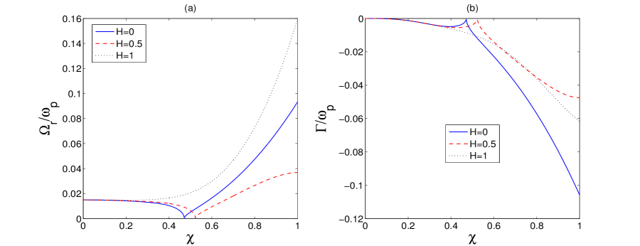
Figure 7: The nondimensional frequency shift $\Omega_{r}/\omega_{p}$ and the energy transfer rate $\Gamma/\omega_{p}$ are plotted against the nondimensional carrier wave number $\chi\equiv k\lambda_{D}$ for different values of $H$ as in the legends and for a fixed $\rho_{0}=K=0.1$. The figure is reproduced from Ref. chatterjee2016 .

From the energy conservation law, it is seen that the Langmuir wave energy decays with time due to the nonlocal term $\propto R$ of the NLS equation (125) associated with the group velocity resonance. Following Ref. chatterjee2015 , approximate soliton solutions of the NLS equation (125) when the wave damping $(\propto R)$ is small can be presented in two different cases. For $PQ>0$, the solution can be written as

$$\phi(\xi,\tau)=\sqrt{\phi_{0}(\xi,0)}\left(1-i\frac{\tau}{\tau_{0}}\right)^{-1/2}\text{sech}~{}{z}\exp(i\theta),$$ (134)

where $z=(\xi-v_{0}\tau)/L$, $\theta=\left[v_{0}\xi+\left(\Omega_{0}-{v_{0}^{2}}/{2}\right)\tau\right]/2P$, with $v_{0},~{}L,~{}\Omega_{0},~{}\theta_{1}$ being constants, and $\tau_{0}$ is given by

$$\tau_{0}^{-1}=\frac{\sqrt{2}R\phi_{0}(\xi,0)}{{\pi}^{3/2}\theta_{1}}\left[\frac{\cosh{(\pi\theta_{1})}-1}{\sinh{\left({\pi\theta_{1}}/{2}\right)}}\right]{\cal{P}}\int_{-\infty}^{\infty}\int_{-\infty}^{\infty}\left(\frac{\text{sech}^{2}z^{\prime}}{z-z^{\prime}}\right)\text{sech}^{2}z\exp(i\theta_{1}z)dzdz^{\prime}.$$ (135)

On the other hand, for $PQ<0$, an approximate solitary wave solution of Eq. (125) is given by chatterjee2015

$$\phi={\phi_{0}(\xi,0)}\left(1-i\frac{\tau}{\tau_{0}}\right)^{-1/2}\text{tanh}{z}\exp(i\theta),$$ (136)

where $\theta$ and $\tau_{0}$ are given by

$$\theta=\frac{1}{2P}\left[v_{0}\xi+\left(2PQ\phi_{0}^{2}(\xi,0)-\frac{v_{0}^{2}}{2}\right)\tau\right],$$ (137)

$$\begin{split}\tau_{0}^{-1}=\left(\frac{2}{\pi}\right)^{3/2}\frac{R\phi_{0}^{2}(\xi,0)\left[1-\cosh(\pi\theta_{2})\right]}{\delta(\tau)(1-\cosh\pi\theta_{2})+\theta_{2}\sinh\left(\frac{\pi\theta_{2}}{2}\right)}{\cal{P}}&\int_{-\infty}^{\infty}\int_{-\infty}^{\infty}\left(\frac{\tanh^{2}z^{\prime}}{z-z^{\prime}}\right)\\ &\times\tanh^{2}z\exp(i\theta_{2}z)dzdz^{\prime},\end{split}$$ (138)

with $\delta(\tau)$ denoting the Dirac delta function and $\theta_{2}$ a real constant.

The decay rate $|\left(1-i\tau/\tau_{0}\right)^{-1/2}|$ can be analyzed for both the cases of $PQ>0$ and $PQ<0$. It is found that the solitary wave amplitude decays with time and the rate is relatively low (compared to the classical case) due to the effects of the quantum particle dispersion.

3.4 Nonlinear Landau damping of electron-acoustic waves due to multi-plasmon resonances

As discussed in Sec. 3.1.2 that in the strong quantum regime, linear Landau resonance is suppressed, however, nonlinear wave-particle interaction is possible due to simultaneous absorption of multiple wave-quanta rather than a single wave quantum at a time. The purpose of this section is to consider this phenomena for a low-frequency electrostatic wave and to show that deviating from the classical or semiclassical regime, not only the phase velocity resonance occurs, there also appear multi-plasmon resonances in the nonlinear regime. As an illustration, we consider the nonlinear wave-particle interaction and evolution of small-amplitude electron-acoustic waves (EAWs) in a partially degenerate plasma with two-temperature electrons and stationary ions. To be brief, in certain environments, e.g., in the interior of giant stars like white dwarfs, gas giants like Jupiter and in laser produced plasmas or ion-beam driven plasmas, the background electrons deviating from the thermodynamic equilibrium can have a relatively high-temperature tail such that they can be grouped into two distinct components with different thermodynamic temperatures $T_{l}$ and $T_{h}$ for low $(\alpha=l)$ and high-temperature $(\alpha=h)$ electrons such that $T_{h}>T_{l}$ and $T_{\alpha}\gtrsim T_{F\alpha}$, where $T_{F\alpha}$ denotes the Fermi temperature of $\alpha$-species electrons. Although, the theory is independent of the background distribution, we consider the Fermi-Dirac distribution at finite temperature $(T_{\alpha}\neq 0)$. The plasmas with two groups of electrons cannot be fully degenerate from quantum mechanical points of view. The other relevant details are given in Ref. misra2021 . From the linear theory of EAWs as in Sec. 2.2, it can be assumed that a low-frequency mode with the dispersion $\omega\propto k$ exists. Also, the Landau damping due to the linear plasmon resonance is weak and the wave damping occurs after a long time of propagation for which the nonlinear evolution of EAWs can be described by the Korteweg-de Vries (KdV) equation. Furthermore, similar to classical plasmas, we assume that the background high-temperature electrons is relatively densely populated compared to the low-temperature species, i.e., $n_{h0}>n_{l0}$. Also, the EAWs are weakly dispersive such that in the regime $\hbar k/m\lesssim v_{tl}$, the Wigner-Moyal equation is still valid and some quantum effects due to the particle’s dispersion become significant in the wave-particle interactions.

The basic equations are the same as Eqs. (63) and (64), i.e., the Wigner-Moyal and Poisson system. Also, the background distributions of partially degenerate electrons are as given by Eq. (65). The conditions for the equilibrium chemical potential $\mu_{\alpha}$ remain also the same as Eqs. (66) and (67) given in Case IV of Sec. 2.2. Having known from the linear theory (Sec. 2.2) that the EAW has a cubic order dispersion and the Landau damping rate is small, we derive an evolution equation for the weakly nonlinear EAWs in a degenerate plasma using the multiple-scale perturbation technique. Some special attention must be devoted to the higher order (in the amplitude) resonances that occur in the Wigner theory. In particular, due to the nonlinearities, we will have Landau resonances with resonant velocities that are shifted an amount $\pm nv_{q}$ in momentum space (See e.g., Ref. brodin2017 ) compared to the resonant velocity of classical theory (i.e., the phase velocity). Here, $n=1$ gives the velocity shift already appeared in the linear theory as described in Sec. 2.2. Close to the resonant velocities, the Wigner equation must be analyzed in more detail. In the quantum regime, the classical resonance velocity is changed according to

$$v^{\text{res}}=\frac{\omega}{k}\rightarrow v^{\text{res}}_{\pm n}=\frac{\omega}{k}\pm n\frac{\hbar k}{2m}.$$ (139)

The details of this modification is given in Sec. 3.1.2.

Dividing the velocity space into the resonance and nonresonance regions, using the multiple scale expansion technique which involves the modified Gardner-Morikawa transformation (i.e., $\xi=\epsilon^{1/2}x,~{}\sigma=\epsilon^{1/2}t,~{}\tau=\epsilon^{3/2}t$, where $\epsilon>0$ is a small scaling parameter) the perturbation expansions for the Wigner function $f_{\alpha}$ and the potential $\phi$, and the multi-scale Fourier-Laplace transforms, and following Ref. misra2021 we obtain the following modified KdV equation with nonlinear Landau damping $\propto\Gamma$ (For details, see Ref. misra2017 ).

$$\frac{\partial\phi}{\partial\tau}+A\frac{\partial^{3}\phi}{\partial\zeta^{3}}+B\phi\frac{\partial\phi}{\partial\zeta}+\Gamma{\cal P}\int_{-\infty}^{\infty}\frac{\partial\phi^{2}\left(\zeta^{\prime},\tau\right)}{\partial\zeta^{\prime}}\frac{1}{\zeta-\zeta^{\prime}}d\zeta^{\prime}=0,$$ (140)

where $\zeta=\xi-v_{p}\sigma$ with $v_{p}$ denoting the phase velocity of EAWs and the coefficients of the KdV equation are $A=1/P$, $B=Q/P$ and $\Gamma=R/P$, given by,

$$\Re P=-\frac{6\pi e^{2}}{m}\sum_{\alpha=l,h}\frac{n_{\alpha 0}T_{\alpha}e^{\xi_{\alpha}}}{v_{F\alpha}T_{F\alpha}}\left[\frac{5(v_{p}^{2}-v_{q}^{2})+2v_{p}v_{t\alpha}}{(v_{p}^{2}-v_{q}^{2})^{2}}\right],$$ (141)

$$\Im P=-6(v_{p}-v_{q})\frac{\pi^{2}e^{2}}{\hbar k}\sum_{\alpha=l,h}\frac{n_{\alpha 0}T_{\alpha}e^{\xi_{\alpha}}}{v_{F\alpha}T_{F\alpha}v_{t\alpha}^{2}}\exp\left\{-\left(\frac{v_{p}-v_{q}}{v_{t\alpha}}\right)^{2}\right\},$$ (142)

$$Q=-\frac{24\pi me^{3}}{(\hbar k)^{3}}\frac{v_{p}^{2}+4v_{q}^{2}}{\lambda(v_{p}^{2}-4v_{q}^{2})}\sum_{\alpha=l,h}\frac{n_{\alpha 0}T_{\alpha}v_{t\alpha}}{v_{F\alpha}T_{F\alpha}}e^{\xi_{\alpha}},$$ (143)

$$R=\frac{6\pi^{2}me^{3}}{(\hbar k)^{3}}\sum_{\alpha=l,h}\frac{n_{\alpha 0}T_{\alpha}}{v_{F\alpha}T_{F\alpha}}e^{\xi_{\alpha}}\left[\exp\left\{-\left(\frac{v_{p}-2v_{q}}{v_{t\alpha}}\right)^{2}\right\}-2\exp\left\{-\left(\frac{v_{p}}{v_{t\alpha}}\right)^{2}\right\}\right].$$ (144)

The expression for the phase velocity $v_{p}$ can be obtained from the linear dispersion relation [Case IV, Eq. (75)] by considering the limit $k\rightarrow 0$. We also note that $P$ becomes complex due to the one plasmon resonance (linear), and so are the dispersive $(\propto A)$, local nonlinear $(\propto B)$, and the nonlocal nonlinear $(\propto\Gamma)$ terms. The latter, however, appears due to the phase velocity and multi-plasmon resonances. Such resonances are noted in Ref. misra2021 with poles at $v=\omega/k\pm nv_{q}$, where $n=0,1,2$, in the integrals appearing in certain expressions for the second order perturbations, namely,

$$\int_{-\infty}^{\infty}\left[\frac{1}{(v-\omega/k-v_{q})^{2}}-\frac{1}{(v-\omega/k+v_{q})^{2}}\right]f_{\alpha}^{(0)}dv,$$ (145)

$$\int_{-\infty}^{\infty}\left(\frac{1}{v-\omega/k-2v_{q}}+\frac{1}{v-\omega/k+2v_{q}}-\frac{2}{v-\omega/k}\right)f_{\alpha}^{(0)}(v)dv.$$ (146)

It is interesting to note that although the form of the KdV equation (140) looks similar to that first obtained by Ott and Sudan ott1969 and later by many authors (See, e.g., Refs. vandam1973 ; barman2017 ) in classical/semiclassical plasmas, the Landau damping term $\propto\Gamma$ appears here as nonlinear due to the phase velocity resonance as well as the two-plasmon resonance processes in the wave-particle interactions. The appearance of such a nonlocal nonlinearity not only modifies the propagation of EAWs but also introduces a new wave damping mechanism. From the reduced expression of $R$ [Eq. (144)] it is evident that the contribution of the two-plasmon resonance is higher than that of the phase velocity resonance, implying that the two-plasmon resonance process is the dominant wave damping mechanism for EAWs.

Meanwhile, the KdV equation (140) conserves the total number of particles, however, the wave energy decays with time misra2021 , i.e.,

$$\frac{\partial}{\partial\tau}\int_{-\infty}^{\infty}|\phi(\zeta,\tau)|^{2}d\zeta\leq 0.$$ (147)

So, a steady-state solution of Eq. (140) with finite wave energy does not exist implying that the wave amplitude will tend to decay due to the nonlinear resonance. In this context, an approximate solitary wave solution of Eq. (140) can be obtained similar to Ref. misra2021

$$\phi_{0}(\tau)=\phi_{00}\left(1+\frac{\tau}{\tau_{0}}\right)^{-2/3},$$ (148)

where

$$\tau_{0}^{-1}=\frac{3}{4}\Gamma\sqrt{\frac{B}{3A}}\phi_{00}^{3/2}{\cal P}\int_{-\infty}^{\infty}\int_{-\infty}^{\infty}\text{sech}^{2}z\frac{\partial}{\partial z^{\prime}}\left(\text{sech}^{4}z^{\prime}\right)\frac{dzdz^{\prime}}{z-z^{\prime}}\approx 2\Gamma\sqrt{\frac{B}{3A}}\phi_{00}^{3/2},$$ (149)

where the Cauchy principal value is evaluated as $\approx 2.8$. From Eq. (148) it is clear that the nonlinear Landau damping indeed causes the wave amplitude to decay with time $\sim(\tau+\tau_{0})^{-2/3}$ which is a bit slower than that $\sim(\tau+\tau_{0})^{-2}$ predicted by Ott and Sudan ott1969 in classical plasmas.

Some important points are to be noted. Since the KdV equation accounts for upto the second order perturbations, the lower resonance velocity is due to the two-plasmon processes and it gives the dominant wave-damping mechanism in the description of EAWs in the strong quantum regime. In the model, the plasmas are not in thermodynamic equilibrium. However, the theory of EAWs can be studied with the background distribution of electrons in thermodynamic equilibrium (i.e., for a single species with finite thermal velocity). For such a background distribution [Eq. (65)] the EAWs tend to have a higher Landau damping rate, making the nonlinear analysis less important.

3.5 Nonlinear Landau damping of Langmuir wave envelopes due to multiplasmon resonances

We turn our attention again to the nonlinear evolution of Langmuir wave envelopes, however, in the strong quantum regime. Specifically, we will consider the wave-particle interaction and the amplitude modulation of Langmuir wave envelopes in a fully degenerate plasma, and focus on the regime $k<k_{\text{cr}}$ where the linear damping is forbidden. Here, $k_{\text{cr}}$ is some critical value of the wave number $k$ such that $\hbar k\sim mv_{F}$ holds. The basic equations are the Wigner-Moyal equation coupled to the Poisson equation [cf. Eqs. (21) and (22)], i.e.,

$$\frac{\partial f}{\partial t}+v\frac{\partial f}{\partial x}-\frac{em}{2i\pi\hbar^{2}}\int\int dx_{0}dv_{0}e^{im_{\alpha}(v-v_{0})x_{0}/\hbar}\left[\phi\left(x+\frac{x_{0}}{2}\right)-\phi\left(x-\frac{x_{0}}{2}\right)\right]f(x,v_{0},t)=0,$$ (150)

$${\frac{\partial^{2}\phi}{\partial x^{2}}}=\frac{e}{\varepsilon_{0}}\left(\int fdv-n_{0}\right),$$ (151)

where $n_{0}$ is the background number density of electrons and ions. In a fully degenerate plasma, the background distribution of electrons is given by the Fermi-Dirac pressure [cf. Eq. (34)]

$$f_{0}(v)=\left\{\begin{array}[]{cc}\left[{2\pi m^{3}}/{(2\pi\hbar)^{3}}\right](v_{F}^{2}-v^{2}),&|{v}|\leq v_{F}\\ 0,&|{v}|>v_{F}.\end{array}\right.$$ (152)

Introducing the multiple space-time scales with the stretched coordinates $x\rightarrow x+\epsilon^{-1}\eta+\epsilon^{-2}\zeta,~{}~{}t\rightarrow t+\epsilon^{-1}\sigma$, the perturbation expansion for $f(\mathbf{v},x,t)$ and $\phi(x,t)$ with a scaling parameter $\epsilon$, and further expanding the harmonic components of $f$ and $\phi$ in terms of Fourier-Laplace integrals chatterjee2015 ; chatterjee2016 ; ichikawa1974 we obtain the following nonlinear Schrödinger (NLS) equation for the evolution of Langmuir wave envelopes in a fully degenerate plasma misra2017 .

$$i\frac{\partial\phi}{\partial\tau}+P\frac{\partial^{2}\phi}{\partial\xi^{2}}+Q|\phi|^{2}\phi+\frac{R}{\pi}\mathcal{P}\int\frac{|\phi(\xi^{\prime},\tau)|^{2}}{\xi-\xi^{\prime}}\phi d\xi^{\prime}=0,$$ (153)

Here, $\xi=\eta-v_{g}\sigma$ with $v_{g}$ denoting the group velocity of the envelope, given by, $v_{g}=\lambda_{1}/\lambda_{2}$, where

$$\lambda_{1}=2-\frac{4\pi e^{2}}{mk^{2}}\int_{C}\frac{v_{p}^{2}-v^{2}+v_{q}^{2}}{{\left\{(v_{p}-v)^{2}-v_{q}^{2}\right\}}^{2}}f_{0}(v)dv,~{}\lambda_{2}=-\frac{8\pi e^{2}}{mk^{2}}\int_{C}\frac{v_{p}-v}{{\left\{(v_{p}-v)^{2}-v_{q}^{2}\right\}}^{2}}f_{0}(v)dv.$$ (154)

The coefficients of the dispersion (group velocity), cubic nonlinear (local), nonlocal nonlinear terms, respectively, are $P,~{}Q$ and $R$, given by $P\equiv(1/2)\partial^{2}\omega/\partial k^{2}=\beta/\alpha,~{}Q=\gamma/\alpha$ and $R=D/\alpha$, where

$$\alpha=-\frac{8\pi e^{2}}{mk}\int_{C}\frac{v_{p}-v}{\left[(v_{p}-v)^{2}-v_{q}^{2}\right]^{2}}f_{0}(v)dv,$$ (155)

$$\beta=1+\frac{4\pi e^{2}}{\hbar k^{3}}\int_{C}\left[\frac{\left(v-v_{q}-v_{g}\right)^{2}}{\left(v_{p}-v+v_{q}\right)^{3}}-\frac{\left(v+v_{q}-v_{g}\right)^{2}}{\left(v_{p}-v-v_{q}\right)^{3}}\right]f_{0}(v)dv$$ (156)

$$\gamma=\left(\frac{1}{4}\frac{AA_{1}}{\hbar}-\frac{1}{2\hbar^{2}}B+C\right)k^{2},$$ (157)

$$D= -\frac{4\pi e^{4}}{m\hbar^{2}k^{2}}\int_{\gamma}\left[\delta\left\{v-\left(v_{p}-3v_{q}\right)\right\}\frac{v-v_{g}+v_{q}}{\left(v_{p}-v-v_{q}\right)^{3}\left(v-v_{g}+2v_{q}\right)}\right.$$ (158)

$$\left.+2\delta(v-v_{g})v_{q}\frac{\left\{\left(v_{p}-v\right)^{2}+v_{q}^{2}\right\}}{\left\{\left(v_{p}-v\right)^{2}-v_{q}^{2}\right\}^{3}}\right]f_{0}(v)dv.$$

The expressions for $A,~{}A_{1},~{}B,$ and $C$ in $\gamma$ are given in Appendix A. Also, the reduced expressions for $\alpha,~{}\beta$, $\gamma$ and $D$ are given in Appendix B.

We note that the integrals in $\alpha$ and $\beta$ do not have any pole except at the linear resonant velocities $v=v^{l}_{res}\equiv v_{p}\pm v_{q}$ which lie outside the regime of interest $k<k_{cr}$, and accordingly, the group velocity dispersion $P$ does not have any resonance contribution in the regime. Furthermore, inspecting the denominators of different expressions for $A,~{}A_{1},~{}B$ and $C$ in $\gamma$, we find that only the two- and three-plasmon resonances can occur at $v_{\mathrm{res}}^{n}=v_{p}-nv_{q}$ for $n=2,3$. Thus, in contrast to classical chatterjee2015 or semiclassical chatterjee2016 plasmas, the nonlinear coefficient $Q$ of the NLS equation is significantly modified by the Landau resonances due to the two- and three-plasmon processes. Also, both the group velocity resonance (the first term of $D$) and the three-plasmon resonance (the second term of $D$) contribute to and modify the nonlocal coefficient $R\propto D$.

As noted before in Sec. 3.3, the mass and momentum are conserved for the NLS equation (153). However, the wave energy $I_{3}=\int\left(|\partial_{\xi}\phi|^{2}-(|Q/2P|)|\phi|^{4}\right)d\xi$ may not be conserved in presence of the nonlocal nonlinearity chatterjee2015 ; chatterjee2016 . In fact, the time variation of the energy integral

$$\frac{\partial I_{3}}{\partial\tau}=-\frac{R}{\pi}\int s^{2}|\hat{\phi}(s,\tau)|^{2}|\hat{\phi}(-s,\tau)|^{2}ds.$$ (159)

becomes positive or negative according to when $R>0$ or $R<0$. A careful exmanination reveals that $R>0$ in the regime $k<k_{\text{cr}}$ misra2017 . In order to explore the regime in more details, we require the dispersion equation to be reduced in the limit of $k\lambda_{F}\lesssim 1$, i.e., one obtains the same relation as Eq. (37) eliasson2010 ; misra2017 . The expressions for the phase velocity and resonant velocities are obtained from this reduced equation and plotted against the wave number $k$. The results are displayed in Fig. 8.

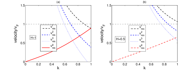
Figure 8: The normalized resonant velocities ($\sim v_{F}$) are plotted against the normalized wave number $k~{}(\sim\lambda_{F}^{-1})$ for two different values of the quantum parameter $H\equiv\hbar\omega_{p}/kv_{F}$ to show different parameter regimes, namely semi-classical (e.g., $0<k\ll 0.59$ for $H=1$), modest quantum ($0<k\lesssim 0.59$ for $H=1$ and $0<k\lesssim 0.75$ for $H=0.5$) and strong quantum ($0.591\lesssim k\lesssim 0.9$ for $H=1$ and $0.75\lesssim k\lesssim 1$ for $H=0.5$) regimes. The figure is reproduced from Ref. misra2017 .

It is seen that there are mainly two parameter regimes: one where the resonant velocities are both the group velocity and the plasmon resonant velocities $v_{\text{res}}^{n}$, $n=2,3$, and the other where only the group velocity resonance is the damping mechanism. The detailed analysis is given in Ref. misra2017 . If $H\sim 1$ there is a region of $k$, i.e., $0<k\lesssim 0.9$ in which the linear resonance is forbidden. However, a subregion of it exists, i.e., $0<k\lesssim 0.59$ in which only the group velocity resonance occurs. The two other subregions exist, namely $0.59\lesssim k\lesssim 0.6953$ and $0.59\lesssim k\lesssim 0.9$. In the former, both the three-plasmon and the group velocity resonances can occur, while in the latter, the group velocity, as well as the two- and three-plasmon resonances can be significant. In this regime, the magnitudes of the coefficients $P,~{}Q$ and $R$ of the NLS equation (153) should be noted. These are, however, useful for the estimation of frequency shift and the rate of energy transfer in the modulation of Langmuir waves, as well as the nonlinear evolution of envelope solitons. On the other hand, multi-plasmon resonances can be forbidden, only the group velocity resonance prevails chatterjee2015 ; chatterjee2016 if $H$ is reduced from $H=1$ to $H=0.5$.

Thus, three regimes may be of interest: (i) Semi-classical regime with $\hbar k\ll mv_{F}$ (i.e., $0<k\ll 0.59$ for $H\sim 1$) where the quantum effect appears only due to the degeneracy of background electrons. The results will be similar to those in Sec. 3.3 or in Ref. chatterjee2016 as the group velocity is only the resonant velocity; (ii) Modest quantum regime with $\hbar k\sim mv_{F}$ and $v_{\text{res}}^{3}>v_{F}$ (i.e., $0<k\lesssim 0.59$ for $H\sim 1$ and $0<k\lesssim 0.75$ for $H\sim 0.5$) in which the resonant velocity is still the group velocity. The results will be similar to those in semiclassical plasmas chatterjee2016 . (iii) Strong quantum regime with $\hbar k\sim mv_{F}$ and $v_{\text{res}}^{3}<v_{F}$ (i.e., $0.591\lesssim k\lesssim 0.9$ for $H=1$ and $0.75\lesssim k\lesssim 1$ for $H=0.5$) in which all the resonant velocities come into the picture. However, the contribution from the three-plasmon resonance becomes higher in magnitude than the group velocity resonance until $v_{\text{res}}^{3}~{}(<v_{F})\gtrsim v^{g}_{\text{res}}$ holds. Thus, in the strong quantum regimes, the three-plasmon resonance plays a decisive role in the nonlinear Landau damping of Langmuir wave envelopes.

Similar to Sec. 3.3 and Refs. chatterjee2016 ; misra2017 , the frequency shift $\Omega_{r}$ and the energy transfer $\Gamma$ rate can be analyzed in the modulation of Langmuir wave envelopes. Although, the forms of the expressions of $\Omega_{r}$ and $\Gamma$ are the same as in classical chatterjee2015 or semiclassical chatterjee2016 plasmas, a significant modification in both the frequency shift and the energy transfer rate is noticed due to the multi-plasmon resonances. The profiles of $\Omega_{r}$ and $\Gamma$ are shown Figs. 9 and 10 especially in the modest quantum and strong quantum regimes (since the semiclassical results are similar to those in Sec. 3.3) for different values of the carrier wave number $k$. It is found that as the value of $k$ decreases from $k=0.59$ to $k=0.5$ and $k=0.4$, the magnitudes of $P$, $Q$ and $R$ are significantly altered leading to an enhancement of the frequency shift, however, the values of $|\Gamma|$ increase until $k=0.5$, and then decrease until $k=0.4$. Thus, in the regime of low wave numbers (below $k=0.5$), although the frequency shift remains high, the magnitude of $\Gamma$ is greatly reduced, implying that the energy transfer rate is relatively low in the semi-classical regimes with $\hbar k/mv_{F}\ll 1$. The energy transfer rate can be maximum near $k=0.5$ where $v_{res}^{3}\gtrsim v_{F}$ holds. On the other hand, in the strong quantum regime $0.591\lesssim k\lesssim 0.9$, it is seen from Fig. 10 that the frequency shift remains high, however, $|\Gamma|$ attains its minimum value. The effect of the three-plasmon resonance is to decrease the values of $\Omega_{r}$ but to increase $|\Gamma|$.

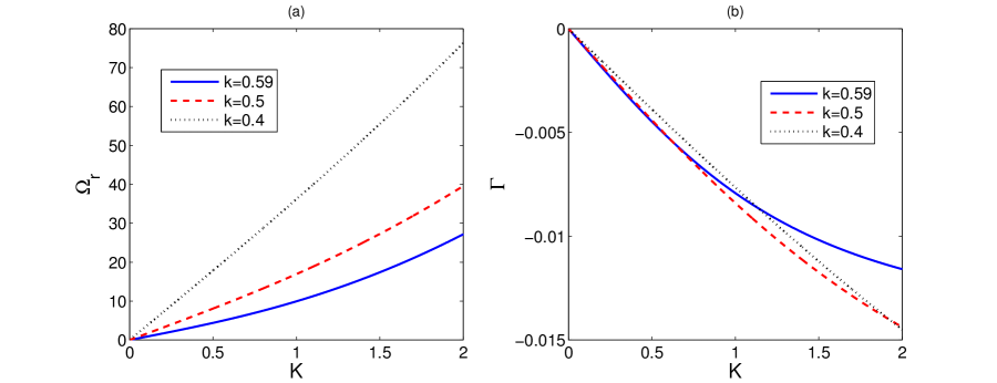
Figure 9: The normalized frequency shift $\Omega_{r}~{}(\sim\omega_{p})$ and the energy transfer rate $\Gamma~{}(\sim\omega_{p})$ are plotted against the normalized wave number of modulation $K~{}(\sim\lambda_{F}^{-1})$ for different values of the carrier wave number $k~{}(\sim\lambda_{F}^{-1})$ that correspond to semi-classical and modest quantum regimes (where $\Im Q=0$). The figure is reproduced from Ref. misra2017 .

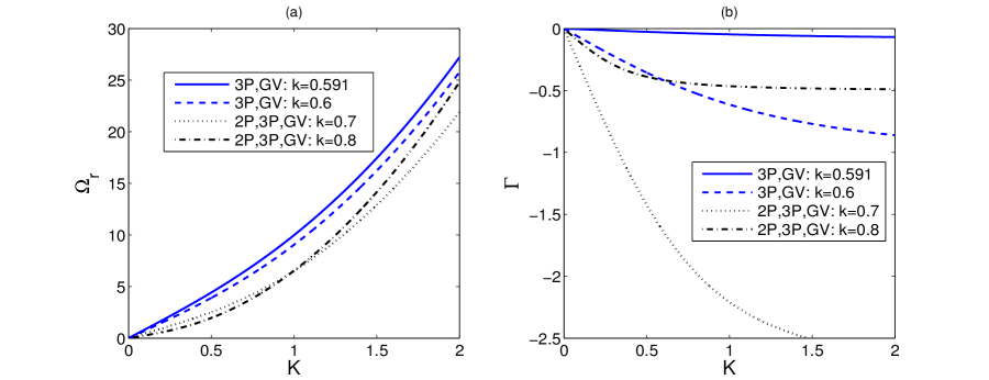
Figure 10: The same as in Fig. 7 but in the strong quantum regime. In the legends, $2P,~{}3P$ and $GV$, respectively, stand for two-plasmon, three-plasmon and group velocity resonance effects. The figure is reproduced from Ref. misra2017 .

It has been established that the nonlocal nonlinearity $(\propto R)$ which appears due to the three-plasmon and group velocity resonances violates the conservation of energy and the wave damping occurs for $R>0$. It is thus imperative to study the effects of the Landau resonances on the profile of an envelope soliton solution of Eq. (153). Following Refs. chatterjee2015 ; chatterjee2016 an approximate soliton solution of Eq. (153) with a small effect of the nonlinear Landau damping $(\propto R)$ can be obtained whose amplitude varies as

$$\phi(\xi,\tau)\propto\sqrt{\phi_{0}(\xi,0)}\left(1-i\frac{\tau}{\tau_{0}}\right)^{-1/2},$$ (160)

where $\tau_{0}$ is some constant inversely proportional to $R$ and $\phi_{0}(\xi,0)$ is the value of $\phi$ at $\tau=0$.

A qualitative plot of the decay rate $DR\equiv|\left(1-i\tau/\tau_{0}\right)^{-1/2}|$ is shown in Fig. 11 in the modest and strong quantum regimes to show the relative importance of the group velocity (solid and dashed lines) and three-plasmon (dotted and dash-dotted lines and as indicated in the figure) resonances. It is found that the decay rate due to the effects of the three-plasmon resonance is faster than that due to the group velocity resonance.

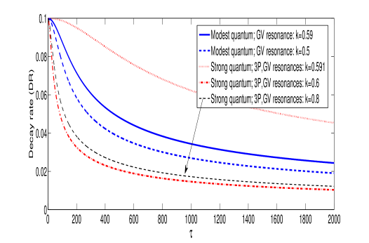
Figure 11: The absolute value of the decay rate $DR\equiv|\left(1-i\tau/\tau_{0}\right)^{-1/2}|$ is shown against the normalized time variable $\tau~{}(\omega_{p}^{-1})$ in different parameter regimes as in the legend. The figure is reproduced from Ref. misra2017 .

3.6 Wave-particle interaction including spin dynamics

While many aspects of wave-particle interaction can be described by the Wigner equation where spin effects are omitted, certain processes must be described by more general equations. Kinetic plasma models including spin effects appear in various degrees of complexity. However, many of the key ingredients in the interaction can be seen already in relatively simple kinetic models including spin. Thus, as a starting point, we will make use of the following approximations:

1. We leave out short-scale (particle dispersive) effects by considering scale lengths much larger than the characteristic de Broglie wavelength. In the absence of spin, such an approximation reduces the Wigner-Moyal equation to the Vlasov equation.

2. We omit weakly relativistic spin effects, i.e., we drop the spin-orbit interaction. For consistency, this also leaves out the effect of Thompson precession and spin polarization currents (only magnetization currents are retained).

3. We make use of the Hartree approximation. While many spin effects are included in the mean-field approximation, the exchange effects (which are also dependent on spin) are not included in the model. This is a consistent approximation since the scaling of the mean-field terms and the exchange contribution with the plasma parameters are different.

Two different but equivalent models, derived from first principles, meeting the above criteria have been derived zamanian2010 ; hurst2014 . We will make use of the governing equations first presented in Ref. zamanian2010 , which slightly corrects an older somewhat simpler model derived using semi-classical arguments brodin2008 . The evolution equation for the distribution function $f(\mathbf{r,v,}\hat{\mathbf{s}},t)$ reads

$$\frac{\partial f}{\partial t}+\mathbf{v}\cdot\nabla_{\mathbf{x}}f+\left[-\frac{e}{m}(\mathbf{E}+\mathbf{v}\times\mathbf{B})+\frac{\tilde{\mu}}{m}\nabla_{\mathbf{x}}\left(\hat{\mathbf{s}}\cdot\mathbf{B}+\mathbf{B}\cdot\nabla_{\hat{\mathbf{s}}}\right)\right]\cdot\nabla_{\mathbf{v}}f+\frac{2\tilde{\mu}}{\hbar}(\hat{\mathbf{s}}\times\mathbf{B})\cdot\nabla_{\hat{\mathbf{s}}}f=0,$$ (161)

with the current density $\mathbf{J}$ in Maxwell’s equations calculated as

$$\mathbf{J} = \mathbf{J}_{f}+\mathbf{J}_{M},$$ (162)

$$= \mathbf{J}_{f}+\nabla_{\mathbf{x}}\times\mathbf{M},$$

$$= -e\int\mathbf{v}fd^{2}sd^{3}v+\nabla_{\mathbf{x}}\times\left(\tilde{\mu}\int 3\hat{\mathbf{s}}fd^{2}sd^{3}v\right).$$

where $\mathbf{J}_{f}$ is the free current density, $\mathbf{M}$ is the magnetization due to the spin, $\tilde{\mu}$ is the electron magnetic moment, and $\mathbf{J}_{M}$ is the magnetization current. The key features of the model are:

1. The phase space is extended with the spin variable $\hat{\mathbf{s}}=(\sin\theta_{s}\cos\varphi_{s},\sin\theta_{s}\sin\varphi_{s},\cos\theta_{s})$, a unit vector on the Bloch sphere that describes the distribution of spin among the particles at given phase space positions. As shown above, when calculating sources in Maxwell’s equations, an extra integration over the Bloch sphere $d^{2}s=\sin\theta_{s}d\theta_{s}d\varphi_{s}$ is required. The integration is usually made in spherical spin coordinates as indicated here and will be used onwards.

2. While the electron magnetic moment is given by the Bohr magneton to a good approximation when the wave particle interaction is considered, it is important to use the QED corrected value $\tilde{\mu}=ge\hbar/4m$, where the electron g-factor is $g=-2.002319$.

3. Since the spin vector has a fixed length, $\nabla_{\hat{\mathbf{s}}}$ is only a gradient on the surface of the Bloch sphere. Hence it is given by $\nabla_{\hat{\mathbf{s}}}=\mathbf{\hat{e}}_{\theta}\partial/\partial\theta_{s}+(1/\sin\theta_{s})\mathbf{\hat{e}}_{\varphi}\partial/\partial\varphi_{s}.$

With the computational aspects of Eq. (161) pointed out we note that the second term inside the square bracket (to the right of the Lorentz force), is the magnetic dipole force, whereas the last term describes the spin precession. Solving Eq. (161) is similar to solving the standard Vlasov equation. For the case of homogeneous linearized theory, a complete description was given in Ref. lundin2010 . We will not repeat the technical details here. Rather, we will just point out the main mechanism affecting wave-particle interaction problems.

Due to the Larmor gyration, as is well-known, for electromagnetic fields the perturbed distribution function $f_{1}$ will have an oscillating dependence on the azimuthal angle in velocity space, i.e.,  $f_{1}\propto\exp(i\varphi_{v})$. For a constant magnetic field $\mathbf{B}_{0}=B_{0}\mathbf{\hat{z}},$ we have $(e/m)(\mathbf{v}\times\mathbf{B}_{0})\cdot\nabla_{\mathbf{v}}=\omega_{c}\partial/\partial\varphi_{v}$, such that $(e/m)(\mathbf{v}\times\mathbf{B}_{0})\cdot\nabla_{\mathbf{v}}f_{1}=i\omega_{c}f_{1}$, where $\omega_{c}=qB_{0}/m$ is the Larmor gyration frequency. Similarly, due to the precession of the spin state, the perturbed distribution function will have the same type of dependence on the spin azimuthal angle  $f_{1}\propto\exp(i\varphi_{s}\dot{)}$. As a result, $(2\tilde{\mu}/\hbar)(\hat{\mathbf{s}}\times\mathbf{B}_{0})\cdot\nabla_{\hat{\mathbf{s}}}f_{1}=i\omega_{cg}f_{1}$, where $\omega_{cg}=(g/2)\omega_{c}$. Since the spin $g$-factor is slightly larger than $2$, the Larmor gyration and the spin precession will not be exactly in sync, which has important consequences.

For the free current contributions, the wave particle interaction terms are similar to the classical case, i.e., there are only quantum corrections affecting the magnitudes of the classical terms. Unless the density is very high and/or the temperature is low, the quantum corrections are relatively modest. However, the expression for the (spin) magnetization current is much different, since it allows for new forms of wave-particle interaction. The reason is that the contribution from $\mathbf{J}_{M}=\nabla_{\mathbf{x}}\times\mathbf{M}$ to the linear conductivity tensor gives rise to new types of resonant denominators in the integrand, related to the slight mismatch between the Larmor gyration frequency and the spin precession frequency outlined above. To be specific, the classical denominators giving raise to wave-particle resonances are modified according to (see Ref. lundin2010 for details)

$$\frac{1}{\omega-k_{z}v_{z}-n\omega_{c}}\rightarrow\frac{1}{\omega-k_{z}v_{z}-n\omega_{c}\pm\omega_{cg}}.$$ (163)

As usual in linearized theory for a magnetized plasma, $n$ is an integer,   and $k_{z}$ is the wavenumber component along the external magnetic field. Firstly, we note that for $k_{z}=0$, contributions from $n=\pm 1$ can be much magnified for frequencies $\omega\simeq\Delta\omega_{c}$, where $\Delta\omega_{c}=\omega_{cg}-\omega_{c}=(g/2-1)\omega_{c}$. As a result, the dispersion relation allows for new wave modes dependent on the spin dynamics. The magnification due to the frequency resonance compensates for a small prefactor for the magnetization current (proportional to $\tilde{\mu}B_{0}/k_{B}T$, which is usually much less than unity), such that $\omega\simeq\Delta\omega_{c}$ applies for most part of the $k-$spectrum. In this sense, these types of spin modes are similar to the Bernstein waves swanson2003 , which tend to have frequencies close to the resonances where $\omega=n\omega_{c}$. The properties of the spin resonance modes have been studied in more detail in Refs. brodin2008 ; zamanian2010 ; asenjo2012 .

It is to be noted that even for plasma parameters with relatively small quantum parameters (with $\tilde{\mu}B_{0}/k_{B}T\ll 1$, $\hbar\omega_{p}/k_{B}T\ll 1$, etc.), and for $\omega$ not close to $\Delta\omega_{c}$, when the dispersion relations are classical to a good approximation, the quantum denominators given in Eq. (163) can have important consequences for wave-particle interactions. The reason is that a strong magnification in the number of resonant particles can compensate for a small prefactor of the magnetization current. To study this and for simplicity, we assume a Maxwell-Boltzmann background distribution. Thus, the Boltzmann factor proportional to the number of resonant electrons is given by $\exp(-v_{\mathrm{rc}n}^{2}/v_{t}^{2})$, where the classical resonant velocities making the denominator zero are given by $v_{\mathrm{rc}n}=$ $(\omega-n\omega_{c})/k_{z}$. By contrast, the spin resonances have (quantum) resonant velocities $v_{\mathrm{rq}n\mathrm{\pm}}=$ $(\omega-n\omega_{c}\pm\omega_{cg})/k_{z}$. The most interesting case here is the quantum resonance $v_{\mathrm{rq}n\mathrm{\pm}}$ with the smallest resonant velocity, giving the maximum number of resonant particles. If the wave frequency $\omega$ is of the order of $\Delta\omega_{c}$ (note that for an electron-proton plasma $\Delta\omega_{c}\sim\omega_{ci}$), this occurs when $n=1$ and we use the positive sign for $\omega_{cg}$, in which case we get

$$v_{\mathrm{rq1+}}=\frac{(\omega-\Delta\omega_{c})}{k_{z}}.$$ (164)

Assuming that $\omega$ is of the same order as $\Delta\omega_{c}$ (but not necessarily very close), in the long wavelength limit (small wave number spectrum regime), we will have the strong inequality $\exp[(\omega-\Delta\omega_{c})^{2}/k_{z}^{2}v_{t}^{2}]\gg\exp\left[-(v_{\mathrm{rc}n})^{2}/v_{t}^{2}\right]$ for all classical resonances (i.e., for any value $n$ for the classical resonant velocity $v_{\mathrm{rc}n}$). A specific case was studied in Ref. zamanian2010 , where the linear damping of ion-cyclotron modes was considered in the limit of parallel propagation. Here, the dominant classical damping mechanism was due to ions. It was found that in the long-wavelength regime, the Boltzmann factor of electrons $\exp[(\omega-\Delta\omega_{c})^{2}/k_{z}^{2}v_{t}^{2}]$ was considerably larger than the Boltzmann factor of ions $\exp[(\omega-\omega_{ci})^{2}/k_{z}^{2}v_{ti}^{2}]$ due to the much lower thermal velocity of ions $v_{ti}\ll v_{t}$. As a result, the damping mechanism shifted from quantum spin-resonance damping, in the long wavelength regime, to classical ion-cyclotron damping in the short wavelength regime.

In the above model (161), the spin resonances only contribute to the cases when a magnetic wave field is present, and thus a constant background field $B_{0}\mathbf{\hat{z}}$ is not sufficient. Specifically, if a Langmuir wave propagates parallel to a constant external magnetic field, there is no perturbed magnetic field. Hence, when Eq. (161) is applied, the magnetization current and the corresponding denominators vanish identically. This is only an approximation, although, the wave-particle resonance of the type (163) is possible even for a purely electrostatic wave field if Eq. (161) is generalized. Including a weakly relativistic correction to Eq. (161), in particular, the spin-orbit interaction, the model is modified according to

$$\hat{\mathbf{s}}\times\mathbf{B\rightarrow}\hat{\mathbf{s}}\times\left(\mathbf{B-}\frac{\mathbf{p}\times\mathbf{E}}{2mc^{2}}\right),$$ (165)

where the extended contribution is referred to as Thomas precession asenjo2012 . We also note that the weakly relativistic theory requires us to change to a distribution function expressed in terms of momentum, i.e., we let $f(\mathbf{r,v,}\hat{\mathbf{s}},t)\rightarrow f(\mathbf{r,p,}\hat{\mathbf{s}},t)$, although we can still use $\mathbf{p/}m\simeq\mathbf{v}$ to leading order. Moreover, we stress that the factor $2$ in the denominator of the second term of the right-hand side of Eq. (165) is consistent with Lorentz invariance (see e.g., Ref. jackson1975 ). Finally, since the particles carrying a spin magnetic dipole is moving, they contribute with a polarization in the laboratory frame asenjo2012 . Thus, the total current density is given by $\mathbf{J}=\mathbf{J}_{f}+\mathbf{J}_{M}+\mathbf{J}_{P}$, with the polarization current, given by,

$$\mathbf{J}_{P}=\frac{\partial\mathbf{P}}{\partial t}=\frac{\partial}{\partial t}\left(3\tilde{\mu}\int\frac{\left(\hat{\mathbf{s}}\times\mathbf{p}\right)}{2m}fd^{2}sd^{3}p\right).$$ (166)

With these changes in place (see Ref. asenjo2012 for the full details of the extended model), it is possible to study spin-resonance damping of Langmuir waves propagating parallel to an external magnetic field. As found in Ref. ekman2021 , even for parameters where the classical electrostatic dispersion relation is a good approximation for the real part of the frequency, for a strong magnetic field (such that $\Delta\omega_{c}$ is of the same order of magnitude as the plasma frequency), the wave-particle damping can be dominated by the spin resonance effect. While the physics is much different (electrostatic waves rather than electromagnetic), the result is similar to the preceding case. That is, in the long wavelength regime, the number of resonant particles for the spin resonance is much higher than that for the classical resonance. This leads to spin resonance damping dominating for long wavelengths, whereas classical wave-particle damping dominates for shorter wavelengths.

While we have focused on the new wave-particle interaction resonances [as seen in Eq. (163) induced by the spin effects, it should be noted that spin dynamics can influence wave-particle dynamics through other mechanisms. For example, when ultra-strong magnetic fields are present, relativistic Landau quantization will give an increased effective mass to electrons in the higher energy state, which affect the wave-particle resonances, see e.g. Ref. alnaseri2020 . It should be stressed, however, that most other mechanisms require either very strong magnetic fields, low temperatures and/or high plasma densities to be significant.

4 Summary and discussion

In this review paper, we have presented a contemporary theoretical knowledge on the wave-particle interactions and Landau damping of electrostatic waves in quantum plasmas. We have restricted our discussion to the resonant interactions of both the linear and nonlinear electrostatic waves, especially Langmuir waves and electron/ion-acoustic waves in semiclassical and relativistic/nonrelativistic quantum plasma regimes. The characteristics and consequences of wave-particle interaction including the spin dynamics are also presented. We have started with the basic concepts of plasma oscillation, wave-particle interactions and the Landau’s linear treatment on wave damping in classical plasmas. Before moving on to nonlinear regimes, we have demonstrated the linear theory of Landau damping in non-relativistic and relativistic quantum plasmas with different distributions of background electrons that are relevant to nondegenerate semiclassical plasmas and degenerate quantum plasmas. The occurrence of different resonance processes and the wave damping associated with them are noted and discussed. It is elucidated that while the phase velocity resonance is still the wave damping mechanism in classical and semiclassical plasmas, the resonant velocity in the quantum regime is, however, shifted by the velocity associated with the plasmon quanta (quantum modified Cherenkov resonance). The dispersion relations for electrostatic modes and the Landau damping rates obtained in different cases are compared and analyzed. We have also discussed the significance of spin effects on the wave-particle interactions in spin plasmas. It is shown that new wave eigenmodes exist as well as new types of wave-particle resonances can occur that typically depend on the anomalous magnetic moment of charged particles.

Going beyond the linear theory, we have discussed the wave-particle interactions for homogeneous plasma waves as well as for localized waves in both the weak and strong quantum regimes. It is found that in the weak quantum regime, not only a transition from the classical to the quantum regime in nonlinear Landau damping occurs, several other new features also take place including the quantum modified bounce frequency and the occurrence of bounce-like amplitude oscillations. On the other hand, the linear damping can be suppressed and the nonlinear multi-plasmon resonance can emerge in the strong quantum regime. We have also considered the evolution of ion-acoustic waves and the modulation of Langmuir wave envelopes in the weak quantum regimes separately. It is shown that similar to classical plasmas, the resonant velocities are still the phase velocity or the group velocity. However, the quantum recoil effect significantly modifies the wave dispersion and nonlinearities and hence the Landau damping rates. Also, discussed are the effects of multi-plasmon resonances on the modulation of Langmuir wave envelopes and low-frequency electron-acoustic waves in the nonlinear regime. It is found that in contrast to classical and semiclassical plasmas, the multi-plasmon resonance is the dominant wave damping mechanism in the nonlinear evolution of electrostatic solitary waves.

The wave-particle interaction is a very vast area of plasma physics. It is extremely rich and vibrant, and it holds great promise for various interesting and important applications including laser-based inertial plasma fusion and the laser-based plasma compression schemes as well as in high-energy density plasmas such as those in compact astrophysical objects (e.g., interior of white dwarf stars). Recently, the quantum kinetic theory of electron plasma waves has been advanced to take into account both electron and photon Landau damping in presence of an arbitrary spectrum of electromagnetic waves mendonca2016 . The results could be relevant in different physical situations such as the early universe and those mentioned before. So, a possible extension of this study to relativistic quantum plasmas especially in the nonlinear regime could be interesting due to a possible overlap between the two resonance processes. In spin plasmas, we have limited our discussion to wave-particle interactions in the weak quantum regime where the typical length scale of oscillation is larger than the thermal de Broglie wavelength and the Zeeman energy is smaller than the particle’s thermal energy. Thus, generalizing the theory in the extended quantum regime where the Zeeman energy is comparable or larger than the thermal energy for which the Landau quantization may enter the picture could be a problem of promising research.

A large number of wave-particle coupling processes and/or applications have not been discussed in this paper although they may be of importance to plasma physics communities. One area where the Landau damping due to the light-matter interactions (surface plasmons in metal structures) plays a vital role in the dissipation mechanism of surface plasmon polaritons misra2020 and provides an intrinsic limitation to plasmonics technology moghadam2021 ; abdikian2017 . Such an investigation requires the development of quantum-mechanical theory and is important for understanding of the underlying physical mechanisms for increasing lifetime of surface plasmons, and providing guidelines in the future design of plasmonic devices li2013 ; shahbazyan2016 . Another area where the resonant quantum particles interacting with the wave can lead to the bump-on-tail and two-stream instabilities, as well as the particle trapping daligault2014 and the formation of phase space structures and wave turbulence to be observed in future experiments haas2008 . Furthermore, other domains of wave-particle interactions which have been left out include the neutrino Landau damping mendonca2000 the Landau damping of electron plasma waves in stimulated Raman and Brillouin scattering bers2009 , quantum two-stream instability liang2021 , and wakefield acceleration brodin2013 in quantum plasmas. Also, interesting and related phenomena referred to as anomalous Landau damping trott2018 can also occur in non-Fermi Liquids. However, such phenomena is beyond the scope of the present review.

Finally, we would like to point out that phenomena similar to Landau damping occur in many fields besides plasma physics. Whenever a fundamental wave mode interacts with a continuous spectrum of oscillators, the dynamics will resemble many of the features that have been studied in the manuscript. To appreciate the ubiquitousness of the Landau mechanism, let us point out a few different examples throughout physics as well as in other fields of science. In plasma physics, the same mathematical structure as in Landau damping is seen for example in mode conversion problem sedlacek1971 . In other fields of physics, Landau type of damping occurs in contexts such as superfluidity fak1990 , Bose-Einstein condensates shchedrin2018 ; mendonca2018 , accelerators herr2013 , and quark physics baier1992 . Moreover, very similar phenomena can occur in biological systems, e.g., in the flashing of fireflies buck1988 and in the periodic firing of the pacemaker cells winfree1980 . The above is by no means a complete list, but it should be clear that linear and nonlinear wave-particle mechanisms can be found very broadly in many fields of natural sciences. The expressions appearing in Sec. 3.5

Appendix A Expressions for $A,~{}A_{1},~{}B$ and $C$ in $\gamma$

$$A=-\frac{16\pi e^{3}}{A_{0}m^{2}k^{3}}{\int_{C}\frac{(v_{p}-v)\left[(v_{p}-v)^{2}+\frac{v_{q}^{2}}{2}\right]}{\left\{(v_{p}-v)^{2}-v_{q}^{2}\right\}^{2}\left\{\left(v_{p}-v+v_{q}\right)^{2}-v_{q}^{2}\right\}\left\{\left(v_{p}-v-v_{q}\right)^{2}-v_{q}^{2}\right\}}F^{(0)}(v)dv},$$ (167)

where

$$A_{0}={1-\frac{\pi e^{2}}{k^{2}m}\int_{C}\frac{F^{(0)}(v)}{(v_{p}-v)^{2}-\left(2v_{q}\right)^{2}}}dv.$$ (168)

Also,

$$A_{1}=-{12\pi e^{3}}\frac{\hbar}{k^{2}m^{2}}\left[\int_{C}\frac{1}{\left\{\left(v_{p}-v+v_{q}\right)^{2}-4v_{q}^{2}\right\}\left\{\left(v_{p}-v-v_{q}\right)^{2}-4v_{q}^{2}\right\}dv}\right.$$

$$\left.+\frac{3}{2}\int_{C}\frac{\left[(v_{p}-v)^{2}+v_{q}^{2}\right]}{\left\{(v_{p}-v)^{2}-4v_{q}^{2}\right\}\left\{\left(v_{p}-v+2v_{q}\right)^{2}-v_{q}^{2}\right\}\left\{\left(v_{p}-v-2v_{q}\right)^{2}-v_{q}^{2}\right\}}\right]F^{(0)}(v)dv,$$

$$B=\frac{4\pi e^{4}}{k^{4}m}\int_{C}\left[\frac{1}{\left\{v_{p}-v+2v_{q}\right\}\left\{v_{p}-v+v_{q}\right\}\left\{\left(v_{p}-v+2v_{q}\right)^{2}-v_{q}^{2}\right\}}\right.$$

$$\left.+\frac{1}{\left\{v_{p}-v-2v_{q}\right\}\left\{v_{p}-v-v_{q}\right\}\left\{\left(v_{p}-v-2v_{q}\right)^{2}-v_{q}^{2}\right\}}\right.$$

$$\left.-\frac{2}{\left\{(v_{p}-v)^{2}-v_{q}^{2}\right\}^{2}}\right]F^{(0)}(v)dv,$$

$$C(k,\omega;v_{g})=-\frac{4\pi e^{4}}{m\hbar^{2}k^{2}}\int_{C}\frac{1}{(v_{p}-v)^{2}-v_{q}^{2}}\frac{I(v)}{v-v_{g}}dv$$

$$=-\frac{4\pi e^{4}}{m\hbar^{2}k^{4}}\int_{C}\left[\frac{v-v_{g}-v_{q}}{\left\{\left(v_{p}-v+2v_{q}\right)^{2}-v_{q}^{2}\right\}\left(v_{p}-v+v_{q}\right)^{2}\left(v-v_{g}-2v_{q}\right)}\right.$$

$$\left.-\frac{v-v_{g}+v_{q}}{\left\{\left(v_{p}-v-2v_{q}\right)^{2}-v_{q}^{2}\right\}\left(v_{p}-v-v_{q}\right)^{2}\left(v-v_{g}+2v_{q}\right)}\right.$$

$$\left.-2v_{q}\frac{\left\{\left(v_{p}-v\right)^{2}+v_{q}^{2}\right\}}{(v-v_{g})\left\{\left(v_{p}-v\right)^{2}-v_{q}^{2}\right\}^{3}}-4v_{q}\frac{v_{p}-v}{\left\{\left(v_{p}-v\right)^{2}-v_{q}^{2}\right\}^{3}}\right]F^{(0)}(v)dv,$$

where

$$I(v)=\frac{1}{k^{2}}\left[\left(v-v_{g}+v_{q}\right)\frac{f^{(0)}\left(v+2v_{q}\right)-f^{(0)}(v)}{{\left\{v_{p}-\left(v+v_{q}\right)\right\}}^{2}}+\left(v-v_{g}-v_{q}\right)\frac{f^{(0)}(v)-f^{(0)}\left(v-2v_{q}\right)}{{\left\{v_{p}-\left(v-v_{q}\right)\right\}}^{2}}\right].$$ (169)

Appendix B Reduced expressions for $\alpha,~{}\beta,~{}\gamma$ and $D$ with the Fermi distribution at zero temperature

$$\alpha=-\frac{8m\omega_{p}^{2}}{3\hbar k^{2}v_{F}^{3}}\sum_{j=\pm 1}\left(v_{p}+jv_{q}\right)\log\left|\frac{v_{p}+jv_{q}-v_{F}}{v_{p}+jv_{q}+v_{F}}\right|,$$ (170)

$$\begin{split}&\beta=1-\frac{3m\omega_{p}^{2}}{2\hbar k^{3}v_{F}^{2}}\sum_{j=\pm 1}\left[\left\{2\left(v_{p}+jv_{q}\right)+\left(v_{p}-v_{g}\right)\right\}\log\left|\frac{v_{p}+jv_{q}-v_{F}}{v_{p}+jv_{q}+v_{F}}\right|\right.\\ &\left.-\left\{v_{F}^{2}-\left(v_{p}+jv_{q}\right)^{2}-2\left(v_{p}+jv_{q}\right)\left(v_{p}-v_{g}\right)\right\}\frac{v_{F}}{v_{F}^{2}-\left(v_{P}+jv_{q}\right)^{2}}+\left(v_{p}-v_{g}\right)\frac{v_{F}\left(v_{p}+jv_{q}\right)}{v_{F}^{2}-\left(v_{p}+jv_{q}\right)^{2}}\right],\end{split}$$ (171)

$$\gamma=\left(\frac{1}{4}\frac{AA_{1}}{\hbar}-\frac{1}{2\hbar^{2}}B+C\right)k^{2},$$ (172)

where

$$\begin{split}&A=-\frac{4em^{2}\omega_{p}^{2}}{A_{0}\hbar^{3}k^{6}v_{F}^{3}}\sum_{j=\pm 1}\left[kv_{F}v_{q}+\frac{\omega_{p}}{6v_{q}}\left\{\left(v_{F}^{2}-\left(v_{p}+jv_{q}\right)^{2}\right)\left(4-\frac{jkv_{q}}{2\omega_{p}}\right)\right.\right.\\ &\left.\left.-6v_{q}\left(v_{p}+jv_{q}\right)\left(1-\frac{jkv_{q}}{2\omega_{p}}\right)\right\}\log\left|\frac{v_{p}+jv_{q}-v_{F}}{v_{p}+jv_{q}+v_{F}}\right|\right.\\ &\left.+\frac{\omega_{p}}{3v_{q}}\left\{v_{F}^{2}-\left(v_{p}+j2v_{q}\right)^{2}\right\}\left(1-\frac{jkv_{q}}{4\omega_{p}}\right)\log\left|\frac{v_{p}+j2v_{q}-v_{F}}{v_{p}+j2v_{q}+v_{F}}\right|\right.\\ &\left.+i\pi v_{q}\omega_{p}\left\{v_{F}^{2}-\left(v_{p}-2v_{q}\right)^{2}\right\}\left(1+\frac{kv_{q}}{4\omega_{p}}\right)\right],\end{split}$$ (173)

with

$$\begin{split}&A_{0}=1-\frac{3\omega_{p}^{2}}{16v_{F}^{2}k^{2}}\left[2-\sum_{j=\pm 1}\frac{jv_{q}}{4v_{F}}\left\{v_{F}^{2}-\left(v_{p}+jv_{q}\right)^{2}\right\}\log\left|\frac{v_{p}+j2v_{q}-v_{F}}{v_{p}+j2v_{q}+v_{F}}\right|\right]\\ &-i\frac{3\pi\omega_{p}^{2}}{64v_{F}^{3}v_{q}k^{2}}\left\{v_{F}^{2}-\left(v_{p}-2v_{q}\right)^{2}\right\}.\end{split}$$ (174)

Also,

$$\begin{split}&A_{1}=-\frac{e}{m}\frac{9\omega_{p}^{2}m^{3}}{4\hbar^{2}v_{F}^{3}k^{5}}\sum_{j=\pm 1}\left[\frac{j}{4}\left\{v_{F}^{2}-\left(v_{p}+jv_{q}\right)^{2}\right\}\log\left|\frac{v_{p}+jv_{q}-v_{F}}{v_{p}+jv_{q}+v_{F}}\right|\right.\\ &\left.-\frac{2j}{3}\left\{v_{F}^{2}-\left(v_{p}+j3v_{q}\right)^{2}\right\}\log\left|\frac{v_{p}+j3v_{q}-v_{F}}{v_{p}+j3v_{q}+v_{F}}\right|+j\left\{v_{F}^{2}-\left(v_{p}+j2v_{q}\right)^{2}\right\}\log\left|\frac{v_{p}+j2v_{q}-v_{F}}{v_{p}+j2v_{q}+v_{F}}\right|\right]\\ &-i\frac{9\pi\omega_{p}^{2}}{16v_{F}^{3}k^{3}}\frac{e}{v_{q}^{2}}\left[\frac{2}{3}\left\{v_{F}^{2}-\left(v_{p}-3v_{q}\right)^{2}\right\}-\left\{v_{F}^{2}-\left(v_{p}-2v_{q}\right)^{2}\right\}\right],\end{split}$$ (175)

$$\begin{split}&B=-\frac{e^{2}}{k^{7}}\frac{3\omega_{p}^{2}m^{3}}{2v_{F}^{3}\hbar^{3}}\sum_{j=\pm 1}\left[16v_{F}v_{q}+4\left\{v_{F}^{2}-\left(v_{p}+j2v_{q}\right)^{2}\right\}\log\left|\frac{v_{p}+j2v_{q}-v_{F}}{v_{p}+j2v_{q}+v_{F}}\right|\right.\\ &\left.+\left\{v_{F}^{2}-\left(v_{p}+j3v_{q}\right)^{2}\right\}\log\left|\frac{v_{p}+j3v_{q}-v_{F}}{v_{p}+j3v_{q}+v_{F}}\right|-\left\{v_{F}^{2}-\left(v_{p}+jv_{q}\right)^{2}-8jv_{q}\left(v_{p}+jv_{q}\right)\right\}\log\left|\frac{v_{p}+jv_{q}-v_{F}}{v_{p}+jv_{q}+v_{F}}\right|\right]\\ &-i\frac{3\pi e^{2}\omega_{p}^{2}}{4k^{4}v_{F}^{3}}\left[-\frac{1}{v_{q}^{3}}\left\{v_{F}^{2}-\left(v_{p}-2v_{q}\right)^{2}\right\}+\frac{1}{4v_{q}^{3}}\left\{v_{F}^{2}-\left(v_{p}-3v_{q}\right)^{2}\right\}\right],\end{split}$$ (176)

$$\begin{split}&C=-\frac{3}{4}\frac{e^{2}}{\hbar^{2}k^{4}}\frac{\omega_{p}^{2}}{v_{F}^{3}}\sum_{j=\pm 1}\left[-\frac{1}{8v_{q}^{3}}\frac{v_{p}+j2v_{q}-v_{g}}{v_{p}+jv_{q}-v_{g}}\left\{v_{F}^{2}-\left(v_{p}+j3v_{q}\right)^{2}\right\}\log\left|\frac{v_{p}+j3v_{q}-v_{F}}{v_{p}+j3v_{q}+v_{F}}\right|+jM_{j}\log\left|\frac{v_{p}+jv_{q}-v_{F}}{v_{p}+jv_{q}+v_{F}}\right|\right.\\ &\left.+jN_{j}\frac{2v_{F}}{v_{F}^{2}-\left(v_{p}+jv_{q}\right)^{2}}-\left(\frac{1}{2v_{q}}\frac{v_{p}-v_{g}}{v_{p}-jv_{q}-v_{g}}-\frac{1}{2}\frac{1}{v_{p}+jv_{q}-v_{g}}-\frac{1}{2v_{q}}\right)\frac{2v_{F}\left(v_{p}+jv_{q}\right)}{v_{F}^{2}-\left(v_{p}+jv_{q}\right)^{2}}\right.\\ &\left.-v_{q}\frac{v_{F}^{2}-\left(v_{g}+jv_{q}\right)^{2}}{\left(v_{p}-jv_{q}-v_{g}\right)^{3}\left(v_{p}+jv_{q}-v_{g}\right)}\log\left|\frac{v_{g}+jv_{q}-v_{F}}{v_{g}+jv_{q}+v_{F}}\right|+\frac{2v_{q}}{k^{2}}\frac{\left\{\left(\omega-kv_{g}\right)^{2}+\frac{\hbar^{2}k^{4}}{4m^{2}}\right\}\left(v_{F}^{2}-v_{g}^{2}\right)}{\left(v_{p}+v_{q}-v_{g}\right)^{3}\left(v_{p}-v_{q}-v_{g}\right)^{3}}log\frac{v_{g}-v_{F}}{v_{g}+v_{F}}\right],\end{split}$$ (177)

with

$$\begin{split}&M_{1,-1}=\frac{1}{4v_{q}^{2}\left(v_{p}-v_{g}\mp 2v_{q}\right)^{2}}\left[\left(v_{p}-v_{g}\mp 3v_{q}\right)\left\{v_{F}^{2}-3\left(v_{p}\pm v_{q}\right)^{2}+2\left(v_{g}\pm v_{q}\right)\left(v_{p}\pm v_{q}\right)\right\}\right.\\ &\left.\mp 4v_{q}\left(v_{p}-v_{g}\mp v_{q}\right)\left(3v_{p}-v_{g}\pm 2v_{q}\right)-2\left(v_{p}\pm v_{q}\right)\left(v_{p}-v_{g}\right)\left(v_{p}-v_{g}\mp 3v_{q}\right)\right.\\ &\left.+\left\{2\left(v_{p}-v_{g}\mp v_{q}\right)+\left(v_{p}-v_{g}\mp 3v_{q}\right)\pm 2\left(v_{q}-v_{g}\right)\left(v_{q}-v_{g}\mp 3v_{q}\right)^{2}\left(\frac{1}{2v_{q}}\mp\frac{1}{v_{p}-v_{g}\mp 2v_{q}}\right)\right\}\left\{v_{F}^{2}-\left(v_{p}\pm v_{q}\right)^{2}\right\}\right]\\ &+\frac{1}{4v_{q}^{2}\left(v_{p}-v_{g}\pm v_{q}\right)^{2}}\left[5\left(v_{p}-v_{g}\pm v_{q}\right)\left\{v_{F}^{2}-\left(v_{p}\pm v_{q}\right)^{2}\right\}\pm 3v_{q}\left\{v_{F}^{2}-\left(v_{p}\pm v_{q}\right)^{2}\right\}\right.\\ &\left.\mp 4v_{q}^{2}\left(v_{p}\pm v_{q}\right)-\left(3v_{p}-3v_{g}\pm 5v_{q}\right)\left\{v_{F}^{2}\mp 2v_{q}\left(v_{p}\pm v_{q}\right)-\left(v_{p}\pm v_{q}\right)^{2}\right\}\right.\\ &\left.+2v_{q}^{2}\frac{v_{F}^{2}-\left(v_{p}\pm v_{q}\right)^{2}}{v_{p}-v_{g}\pm v_{q}}\right]\pm\frac{v_{p}}{v_{q}^{2}},\end{split}$$ (178)

$$\begin{split}&N_{1,-1}=\pm\frac{1}{4v_{q}^{2}\left(v_{p}-v_{g}\mp v_{q}\right)^{2}}\left[2v_{q}\left(v_{p}-v_{g}\mp v_{q}\right)\left\{v_{F}^{2}-3\left(v_{p}\pm v_{q}\right)^{2}-2\left(v_{p}-v_{g}\right)\left(v_{p}\pm v_{q}\right)\right\}\right.\\ &\left.+\left\{v_{F}^{2}-\left(v_{p}\pm v_{q}\right)^{2}\right\}\left(v_{p}-v_{g}\right)\left(v_{p}-v_{g}\mp 3v_{q}\right)\right]\\ &\mp\frac{1}{4v_{q}{\left(v_{p}-v_{g}\mp v_{q}\right)^{2}}}\left[\left(v_{p}-v_{g}\mp 3v_{q}\right)\left\{v_{F}^{2}-\left(v_{p}\pm v_{q}\right)^{2}\right\}\pm 4v_{q}\left(v_{p}\pm v_{q}\right)\left(v_{p}-v_{g}\pm v_{q}\right)\right]\\ &\pm\frac{1}{4v_{q}^{2}}\left[v_{p}\pm v_{q}-\left\{v_{F}^{2}-\left(v_{p}\pm v_{q}\right)^{2}\right\}\right],\end{split}$$ (179)

$$D=\frac{3e^{2}\pi\omega_{p}^{2}}{4k\hbar mv_{F}^{3}}\left[(v_{F}^{2}-v_{g}^{2})\frac{(v_{p}-v_{g})^{2}+v_{q}^{2}}{{\left\{(v_{p}-v_{g})^{2}-v_{q}^{2}\right\}^{3}}}+\frac{1}{8v_{q}^{4}}\left\{v_{F}^{2}-\left(v_{p}-3v_{q}\right)^{2}\right\}\frac{v_{p}-v_{g}-2v_{q}}{v_{p}-v_{g}-v_{q}}\right].$$ (180)

This expression (180) of $D$ is obtained by using the following relations.

$$\lim_{\nu_{g}\rightarrow 0}\frac{1}{\Omega-Kv+i\nu_{g}}=\frac{1}{\Omega-Kv}-i\pi\frac{1}{|K|}\delta\left(v-\frac{\Omega}{K}\right),$$

$$\lim_{\nu_{3}\rightarrow 0}\frac{1}{\omega-kv-3kv_{q}+i\nu_{3}}=\frac{1}{\omega-kv-3kv_{q}}$$

$$-i\pi\frac{1}{|K|}\delta\left(v-v_{p}+3v_{q}\right),$$ (181)

and we have made use of $\Omega/K\rightarrow v_{g}$. The infinitesimal quantities $|\nu_{g}|$ and $|\nu_{3}|$ are taken to anticipate the Landau damping terms associated with the group velocity and three-plasmon resonances.

Thus, the reduced expressions of $P,~{}Q$ and $R$ can be obtained from the relations $P=\beta/\alpha$, $Q=\gamma/\alpha$ and $R=D/\alpha$.

Conflict of interest statement

The authors have no actual or potential conflicts of interest to declare in relation to this article.

References

- (1) H. Haug, S.W. Koch, Quantum Theory of the Optical and Electronic Properties of Semiconductors, 5th edn. (WORLD SCIENTIFIC, 2009). DOI 10.1142/7184. URL https://www.worldscientific.com/doi/abs/10.1142/7184
- (2) P.K. Shukla, B. Eliasson, Physics-Uspekhi 53(1), 51 (2010). DOI 10.3367/ufne.0180.201001b.0055. URL https://doi.org/10.3367/ufne.0180.201001b.0055
- (3) J. Zamanian, M. Marklund, G. Brodin, New Journal of Physics 12(4), 043019 (2010). DOI 10.1088/1367-2630/12/4/043019. URL https://doi.org/10.1088/1367-2630/12/4/043019
- (4) A. Antoniazzi, G.D. Ninno, D. Fanelli, A. Guarino, S. Ruffo, Journal of Physics: Conference Series 7, 143 (2005). DOI 10.1088/1742-6596/7/1/012. URL https://doi.org/10.1088/1742-6596/7/1/012
- (5) B.T. Tsurutani, G.S. Lakhina, Reviews of Geophysics 35(4), 491 (1997). DOI https://doi.org/10.1029/97RG02200. URL https://agupubs.onlinelibrary.wiley.com/doi/abs/10.1029/97RG02200
- (6) R. Koch, Plasma Physics and Controlled Fusion 48(12B), B329 (2006). DOI 10.1088/0741-3335/48/12b/s31. URL https://doi.org/10.1088/0741-3335/48/12b/s31
- (7) N. Thakkar, N.P. Montoni, C. Cherqui, D.J. Masiello, Phys. Rev. B 97, 121403 (2018). DOI 10.1103/PhysRevB.97.121403. URL https://link.aps.org/doi/10.1103/PhysRevB.97.121403
- (8) in Collected Papers of L.D. Landau, ed. by D. TER HAAR (Pergamon, 1965), pp. 445–460. DOI https://doi.org/10.1016/B978-0-08-010586-4.50066-3. URL https://www.sciencedirect.com/science/article/pii/B9780080105864500663
- (9) D. Bohm, E.P. Gross, Phys. Rev. 75, 1851 (1949). DOI 10.1103/PhysRev.75.1851. URL https://link.aps.org/doi/10.1103/PhysRev.75.1851
- (10) N. Van Kampen, Physica 21(6), 949 (1955). DOI https://doi.org/10.1016/S0031-8914(55)93068-8. URL https://www.sciencedirect.com/science/article/pii/S0031891455930688
- (11) K. Case, Annals of Physics 7(3), 349 (1959). DOI https://doi.org/10.1016/0003-4916(59)90029-6. URL https://www.sciencedirect.com/science/article/pii/0003491659900296
- (12) J.H. Malmberg, C.B. Wharton, Phys. Rev. Lett. 13, 184 (1964). DOI 10.1103/PhysRevLett.13.184. URL https://link.aps.org/doi/10.1103/PhysRevLett.13.184
- (13) S. Sarkar, S. Paul, R. Denra, Physics of Plasmas 22(10), 102109 (2015). DOI 10.1063/1.4933041. URL https://doi.org/10.1063/1.4933041
- (14) G. Thejappa, R.J. MacDowall, The Astrophysical Journal 864(2), 122 (2018). DOI 10.3847/1538-4357/aad5e4. URL https://doi.org/10.3847/1538-4357/aad5e4
- (15) D. Chatterjee, A.P. Misra, Physics of Plasmas 23(10), 102114 (2016). DOI 10.1063/1.4964910. URL https://doi.org/10.1063/1.4964910
- (16) B. ELIASSON, P.K. SHUKLA, Journal of Plasma Physics 76(1), 7 (2010). DOI 10.1017/S0022377809990316
- (17) A.P. Misra, D. Chatterjee, G. Brodin, Phys. Rev. E 96, 053209 (2017). DOI 10.1103/PhysRevE.96.053209. URL https://link.aps.org/doi/10.1103/PhysRevE.96.053209
- (18) R.A. Ferrell, Phys. Rev. 107, 450 (1957). DOI 10.1103/PhysRev.107.450. URL https://link.aps.org/doi/10.1103/PhysRev.107.450
- (19) D.B. Melrose, A. Mushtaq, Phys. Rev. E 82, 056402 (2010). DOI 10.1103/PhysRevE.82.056402. URL https://link.aps.org/doi/10.1103/PhysRevE.82.056402
- (20) S. Rightley, D. Uzdensky, Physics of Plasmas 23(3), 030702 (2016). DOI 10.1063/1.4943870. URL https://doi.org/10.1063/1.4943870
- (21) S. Hau-Riege, Examples of X-Ray–Matter Interaction (John Wiley & Sons, Ltd, 2011), chap. 10, pp. 239–261. DOI https://doi.org/10.1002/9783527636365.ch10. URL https://onlinelibrary.wiley.com/doi/abs/10.1002/9783527636365.ch10
- (22) P. Gibbon, Short Pulse Laser Interactions with Matter (PUBLISHED BY IMPERIAL COLLEGE PRESS AND DISTRIBUTED BY WORLD SCIENTIFIC PUBLISHING CO., 2005). DOI 10.1142/p116. URL https://www.worldscientific.com/doi/abs/10.1142/p116
- (23) A.P. Misra, D. Chatterjee, G. Brodin, Physics of Plasmas 28(11), 112102 (2021). DOI 10.1063/5.0061716. URL https://doi.org/10.1063/5.0061716
- (24) J.P. Holloway, J.J. Dorning, Phys. Rev. A 44, 3856 (1991). DOI 10.1103/PhysRevA.44.3856. URL https://link.aps.org/doi/10.1103/PhysRevA.44.3856
- (25) J. Zhu, P. Ji, Plasma Physics and Controlled Fusion 54(6), 065004 (2012). DOI 10.1088/0741-3335/54/6/065004. URL https://doi.org/10.1088/0741-3335/54/6/065004
- (26) G. Brodin, R. Ekman, J. Zamanian, Plasma Physics and Controlled Fusion 60(2), 025009 (2017). DOI 10.1088/1361-6587/aa979d. URL https://doi.org/10.1088/1361-6587/aa979d
- (27) T. O’Neil, The Physics of Fluids 8(12), 2255 (1965). DOI 10.1063/1.1761193. URL https://aip.scitation.org/doi/abs/10.1063/1.1761193
- (28) D.R. Nicholson, (John Wiley & Sons, 1983)
- (29) G. Brodin, J. Zamanian, J.T. Mendonca, Physica Scripta 90(6), 068020 (2015). DOI 10.1088/0031-8949/90/6/068020. URL https://doi.org/10.1088/0031-8949/90/6/068020
- (30) J. Daligault, Physics of Plasmas 21(4), 040701 (2014). DOI 10.1063/1.4873378. URL https://doi.org/10.1063/1.4873378
- (31) N.D. Suh, M.R. Feix, P. Bertrand, Journal of Computational Physics 94(2), 403 (1991). DOI https://doi.org/10.1016/0021-9991(91)90227-C. URL https://www.sciencedirect.com/science/article/pii/002199919190227C
- (32) E. Ott, R.N. Sudan, The Physics of Fluids 12(11), 2388 (1969). DOI 10.1063/1.1692358. URL https://aip.scitation.org/doi/abs/10.1063/1.1692358
- (33) J. W. Vandam, T. Taniuti, Journal of the Physical Society of Japan 35(3), 897 (1973). DOI 10.1143/JPSJ.35.897. URL https://doi.org/10.1143/JPSJ.35.897
- (34) A. Barman, A.P. Misra, Physics of Plasmas 24(5), 052116 (2017). DOI 10.1063/1.4983308. URL https://doi.org/10.1063/1.4983308
- (35) F. Haas, L.G. Garcia, J. Goedert, G. Manfredi, Physics of Plasmas 10(10), 3858 (2003). DOI 10.1063/1.1609446. URL https://doi.org/10.1063/1.1609446
- (36) A. Barman, A.P. Misra, Physics of Plasmas 21(7), 073708 (2014). DOI 10.1063/1.4890571. URL https://doi.org/10.1063/1.4890571
- (37) S. Kumar Tiwari, A. Sen, Physics of Plasmas 23(2), 022301 (2016). DOI 10.1063/1.4941092. URL https://doi.org/10.1063/1.4941092
- (38) Y.H. Ichikawa, Progress of Theoretical Physics Supplement 55, 212 (1974). DOI 10.1143/PTPS.55.212. URL https://doi.org/10.1143/PTPS.55.212
- (39) D. Chatterjee, A.P. Misra, Phys. Rev. E 92, 063110 (2015). DOI 10.1103/PhysRevE.92.063110. URL https://link.aps.org/doi/10.1103/PhysRevE.92.063110
- (40) J. Hurst, O. Morandi, G. Manfredi, P.A. Hervieux, The European Physical Journal D 68, 176 (2014). DOI 10.1140/epjd/e2014-50205-5. URL https://doi.org/10.1140/epjd/e2014-50205-5
- (41) G. Brodin, M. Marklund, J. Zamanian, A. Ericsson, P.L. Mana, Phys. Rev. Lett. 101, 245002 (2008). DOI 10.1103/PhysRevLett.101.245002. URL https://link.aps.org/doi/10.1103/PhysRevLett.101.245002
- (42) J. Lundin, G. Brodin, Phys. Rev. E 82, 056407 (2010). DOI 10.1103/PhysRevE.82.056407. URL https://link.aps.org/doi/10.1103/PhysRevE.82.056407
- (43) D.G. Swanson, (Taylor & Francis Group (CRC Press), 2003). DOI https://doi.org/10.1201/9780367802721
- (44) F.A. Asenjo, J. Zamanian, M. Marklund, G. Brodin, P. Johansson, 14(7), 073042 (2012). DOI 10.1088/1367-2630/14/7/073042. URL https://doi.org/10.1088/1367-2630/14/7/073042
- (45) J.D. Jackson, (John Wiley & Sons, New York, 1975), chap. 11.11, p. 848
- (46) R. Ekman, H. Al-Naseri, J. Zamanian, G. Brodin, The European Physical Journal D 75, 29 (2021). DOI 10.1140/epjd/s10053-020-00021-3. URL https://doi.org/10.1140/epjd/s10053-020-00021-3
- (47) H. Al-Naseri, J. Zamanian, R. Ekman, G. Brodin, Phys. Rev. E 102, 043203 (2020). DOI 10.1103/PhysRevE.102.043203. URL https://link.aps.org/doi/10.1103/PhysRevE.102.043203
- (48) J.T. Mendonça, A. Serbeto, Physica Scripta 91(9), 095601 (2016). DOI 10.1088/0031-8949/91/9/095601. URL https://doi.org/10.1088/0031-8949/91/9/095601
- (49) A.P. Misra, M. Shahmansouri, N. Khoddam, Physica Scripta 96(1), 015601 (2020). DOI 10.1088/1402-4896/abc44d. URL https://doi.org/10.1088/1402-4896/abc44d
- (50) M.M. Moghadam, M. Shahmansouri, Plasmonics 16, 1349 (2021). DOI 10.1007/s11468-021-01401-0. URL https://doi.org/10.1007/s11468-021-01401-0
- (51) A. Abdikian, Z. Ehsan, Physics Letters A 381(35), 2939 (2017). DOI https://doi.org/10.1016/j.physleta.2017.07.020. URL https://www.sciencedirect.com/science/article/pii/S0375960117306849
- (52) X. Li, D. Xiao, Z. Zhang, 15(2), 023011 (2013). DOI 10.1088/1367-2630/15/2/023011. URL https://doi.org/10.1088/1367-2630/15/2/023011
- (53) T.V. Shahbazyan, Phys. Rev. B 94, 235431 (2016). DOI 10.1103/PhysRevB.94.235431. URL https://link.aps.org/doi/10.1103/PhysRevB.94.235431
- (54) F. Haas, B. Eliasson, P.K. Shukla, G. Manfredi, Phys. Rev. E 78, 056407 (2008). DOI 10.1103/PhysRevE.78.056407. URL https://link.aps.org/doi/10.1103/PhysRevE.78.056407
- (55) J.T. MENDONCA, P.K. SHUKLA, R.B. BINGHAM, J.M. DAWSON, L.O. SILVA, Journal of Plasma Physics 64(2), 97–108 (2000). DOI 10.1017/S0022377800008400
- (56) A. Bers, I.P. Shkarofsky, M. Shoucri, Physics of Plasmas 16(2), 022104 (2009). DOI 10.1063/1.3073678. URL https://doi.org/10.1063/1.3073678
- (57) J.H. Liang, T.X. Hu, D. Wu, Z.M. Sheng, Phys. Rev. E 103, 033207 (2021). DOI 10.1103/PhysRevE.103.033207. URL https://link.aps.org/doi/10.1103/PhysRevE.103.033207
- (58) G. BRODIN, A. HOLKUNDKAR, M. MARKLUND, Journal of Plasma Physics 79(4), 377–382 (2013). DOI 10.1017/S0022377813000093
- (59) M.J. Trott, C.A. Hooley, Phys. Rev. B 98, 201113 (2018). DOI 10.1103/PhysRevB.98.201113. URL https://link.aps.org/doi/10.1103/PhysRevB.98.201113
- (60) Z. Sedláček, Journal of Plasma Physics 5(2), 239–263 (1971). DOI 10.1017/S0022377800005754
- (61) B. Fåk, K. Guckelsberger, M. Körfer, R. Scherm, A.J. Dianoux, Phys. Rev. B 41, 8732 (1990). DOI 10.1103/PhysRevB.41.8732. URL https://link.aps.org/doi/10.1103/PhysRevB.41.8732
- (62) G. Shchedrin, D. Jaschke, L.D. Carr, Scientific Reports 8, 11523 (2018). DOI 10.1038/s41598-018-29454-y. URL https://doi.org/10.1038/s41598-018-29454-y
- (63) J.T. Mendonça, H. Terças, A. Gammal, Phys. Rev. A 97, 063610 (2018). DOI 10.1103/PhysRevA.97.063610. URL https://link.aps.org/doi/10.1103/PhysRevA.97.063610
- (64) in Proceedings of the CAS-CERN Accelerator School: Advanced Accelerator Physics, ed. by W. Herr (Geneva: CERN, Geneva, Switzerland, 2014), p. 548. DOI http://dx.doi.org/10.5170/CERN-2014-009
- (65) R. Baier, H. Nakkagawa, A. Niegawa, K. Redlich, Zeitschrift fuer Physik. C 53(3), 433 (1992). DOI 10.1063/1.4890571
- (66) J. Buck, The Quarterly Review of Biology 63(3), 265 (1998). URL https://www.jstor.org/stable/2830425
- (67) A.T. Winfree, Electrical Rhythmicity and Excitability in Cell Membranes (Springer, Berlin, 1980), pp. 315–336