Learning Continuous Representation of Audio
for Arbitrary Scale Super Resolution

Abstract

Audio super resolution aims to predict the missing high resolution components of the low resolution audio signals. While audio in nature is a continuous signal, current approaches treat it as discrete data (i.e., input is defined on discrete time domain), and consider the super resolution over a fixed scale factor (i.e., it is required to train a new neural network to change output resolution). To obtain a continuous representation of audio and enable super resolution for arbitrary scale factor, we propose a method of implicit neural representation, coined Local Implicit representation for Super resolution of Arbitrary scale (LISA). Our method locally parameterizes a chunk of audio as a function of continuous time, and represents each chunk with the local latent codes of neighboring chunks so that the function can extrapolate the signal at any time coordinate, i.e., infinite resolution. To learn a continuous representation for audio, we design a self-supervised learning strategy to practice super resolution tasks up to the original resolution by stochastic selection. Our numerical evaluation shows that LISA outperforms the previous fixed-scale methods with a fraction of parameters, but also is capable of arbitrary scale super resolution even beyond the resolution of training data.

Index Terms—  audio super resolution, speech super resolution, bandwidth extension, implicit neural networks

1 Introduction

Audio super resolution is a task to construct the missing high resolution components of given audio in low resolution. The problem is also known as bandwidth extension and sampling rate conversion (SRC), and has been studied extensively in signal processing community. In early works [1, 2], super-resolution of factor $\frac{L}{M}$ is performed by a sequence of $L$-fold upsampling interpolation, low-pass filtering, and then $M$-fold downsampling. Note that the output quality of non-integer scale algorithm is mainly determined by upsampling method, e.g., spline [3]. Classical approaches for upsampling have been devised with a set of probabilistic models, e.g., Gaussian mixture models [4], hidden Markov models [5] and linear predictive coding [6]. Recently, the advances of deep learning techniques have made remarkable improvement of upsampling, including but not limited to U-Net architecture [7], Generative Adversarial Networks (GANs) [8, 9], and normalizing flows [10]. The existing deep learning methods however focus on the fixed scale super resolution, in which neural network is used to have discrete representation of audio signal only at a given set of coordinates corresponding to the target resolution. However, audio is continuous in time, and this motivates us to obtain a continuous representation of audio signal, which further enables the audio super resolution of arbitrary scale factor. Meanwhile, for the continuous representation of natural data such as images and audio, implicit neural representation is an emerging area where neural network is employed as a representation function mapping from continuous coordinates to the corresponding signals (e.g., RGB value on a pixel in image, and amplitude on a sampling point in audio)  [11, 12, 13, 14].

We propose Local Implicit representation for Super resolution of Arbitrary scale (LISA) to obtain a continuous representation of audio. LISA consists of a pair of encoder and decoder. The encoder corresponds each chunk of audio to a latent code parameterizing a local input signal around the chunk. The decoder takes a continuous time coordinate and the neighboring set of latent codes around the coordinate, and predicts the value of signal at the coordinate. To train such a continuous representation for audio, we devise a self-supervised learning framework. Specifically, after downsampling the training data to the input resolution, we generate super resolution tasks of random scale factors up to the original resolution. As a training objective, we use a stochastic measure of audio discrepancy between the entire reconstructed and original signals in waveform and spectrogram, in which discrepancy closer to the target chunk receives higher random weight so that the local latent code of a chunk captures a characteristic of the global audio signal, while focuses on the local signal around the chunk.

Thanks to the continuous representation, LISA enables the arbitrary scale super resolution, by requesting the prediction of signal for the set of time coordinates corresponding to any arbitrary target resolution. In addition, the proposed method has several advantages in audio super resolution, compared to the existing works on implicit neural representation. In [11], a demonstration of implicit neural representation for audio is provided. However, it requires a training procedure of neural network per signal, whereas our method does not. LISA with local implicit representation is particularly useful in audio super resolution since the encoding and decoding can be performed once a small chunk is obtained, i.e., low latency. The methods of [13, 14] are analog to ours in a sense of localizing implicit representations. However, they are dedicated to computer vision applications such as 3D vision [13] and 2D image [14], while we focus on the local implicit representation of audio. Indeed, our approach includes some specialized features such as the pair of neural encoder and decoder to process audio data and the self-supervised learning with the audio discrepancy. In addition, we discover the advantages of having the local implicit representation in terms of the low latency and the arbitrary scale factor as input audio is often streaming in audio super resolution, while such benefits are overshadowed in computer vision applications since the vision data are given in a lump rather than a streaming fashion. We further describe differences in details in Section 2.

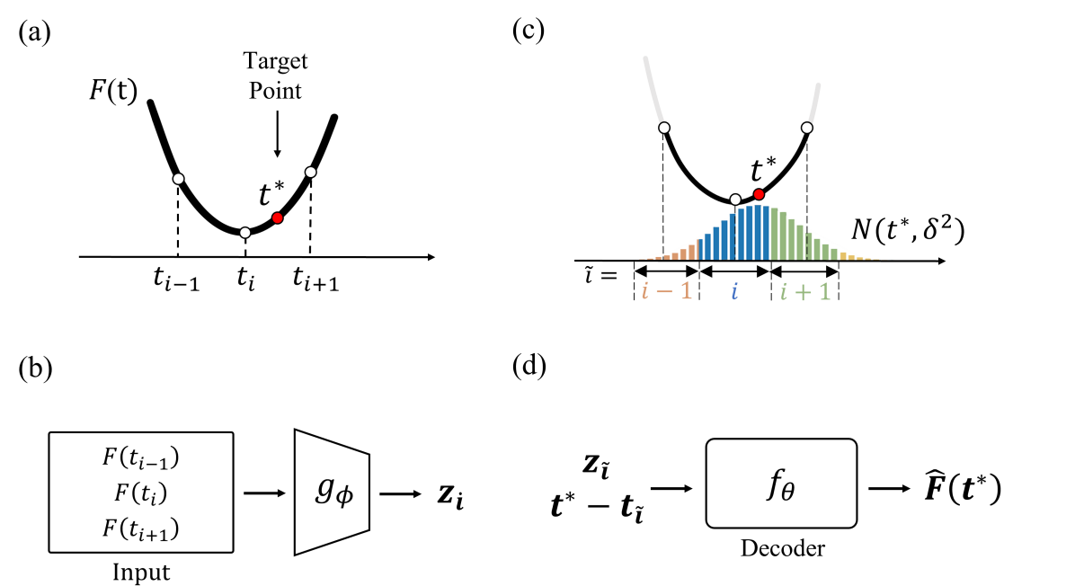
Fig. 1: Model architecture. (a) The white circles denote sampled points of the input signal and the red circle denotes the point of interest. (b) A convolutional encoder extracts local continuous representation. (c) An index ${\tilde{i}}$ is selected stochastically from $\mathcal{N}(t^{*},\delta^{2})$. (d) The amplitude of $t^{*}$ is predicted by the relative distance around $t_{\tilde{i}}$ and a latent code. $z_{\tilde{i}}$ represents a continuous local signal.

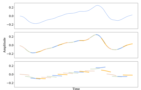
Fig. 2: An example of local continuous representation. (top) target signal (mid) local signals trained with stochastic selection (bottom) local signals trained with local ensemble.

2 Method

Audio in nature is continuous, denoted by $F(t)$ for continuous $t\in\mathbb{R}$, whereas we discretely observe $F(t)$ for $t=t_{i}$’s in every sampling period $\frac{1}{R_{\text{in}}}$, where $R_{\text{in}}>0$ is the input resolution, and $t_{i}$ is the $i$-th temporal coordinate, i.e., $t_{i}-t_{i-1}=\frac{1}{R_{\text{in}}}$. Our method, LISA, aims to obtain continuous representation $\hat{F}(t)$ for continuous $t$ given a local part of discrete samples $F(t_{i})$’s only around $t$ as input so that it provides the arbitrary scale super resolution with low latency. To do so, LISA employs encoder $g_{\phi}$ and decoder $f_{\theta}$ with neural network parameters $\phi$ and $\theta$, respectively. We use encoder $g_{\phi}$ to extract local latent code $z_{i}$ from $(2k+1)$ samples around time $t_{i}$, i.e.,

$$z_{i}:=g_{\phi}(F(t_{i-k}),...,F(t_{i+k}))\;.$$ (1)

Let $i(t)$ be the closest index to $t$, i.e., $i(t):=\operatorname*{arg\,min}_{i}|t-t_{i}|$ where tie breaks with preference to smaller $i$. We denote by $z(t):=(z_{i(t)-1},z_{i(t)},z_{i(t)+1})$ the set of local latent codes corresponding to $t$. Then, LISA represents the signal at any time $t\in\mathbb{R}$ using decoder $f_{\theta}$ as follows:

$$\hat{F}(t):=f_{\theta}(t-t_{i(t)};z(t))\approx{F}(t)\;.$$ (2)

When we want the super resolution from $R_{\text{in}}$ to $R_{\text{out}}$, the output signal is predicted by putting the sequence of time coordinates every $\frac{1}{R_{\text{out}}}$ to $\hat{F}(\cdot)$. We note that ignoring computational cost for encoding and decoding, a theoretical upper bound of latency to predict signal in high resolution around $t$ is only $\frac{k+1}{R_{\text{in}}}$. A graphical illustration in Fig 1 summarizes LISA.

2.1 Model Architecture

Encoder. To induce the temporal correlation in an audio signal, we use convolutional networks for encoder $g_{\phi}$, which produces a latent vector summarizing a few consecutive data points. Our fully convolutional encoder consists of 4 1D-convolution layers with the kernel size of {7, 3, 3, 1} and the channel size of {16, 32, 64, 32}. Note that the kernel size of convolutional network determines the range of receptive field of encoder $g_{\phi}$ in (1), i.e., in our choice, $k=5=3+1+1+0$ as $7=2\cdot 3+1$, $3=2\cdot 1+1$, and $1=2\cdot 0+1$. Note that selecting larger $k$ may force to embed longer pattern inside signal, but it causes longer latency and requires a larger number of parameters.

Decoder. For decoder $f_{\theta}$, we use a 5-layer MLP with ReLU activation, of which input to predict signal at $t$ is the concatenated vector of the relative coordinate $t-t_{i(t)}$ and the set $z(t)$ of local latent codes around $t$. In [11, 15], as a part of empowering representation of features in high frequency, periodic activations, such as sine function, have been proposed instead of ReLU. However, according to our experiment, such periodic activations make the training highly sensitive to initialization and hyperparameters. We hence choose to use ReLU for stable training, and small enough $k$ to express meticulous local representation. The encoder generates the concatenated latent vector $z(t)=(z_{i(t)-1},z_{i(t)},z_{i(t)+1})$, which adds more information on the signal at a small computational cost.

2.2 Training Strategy

To train encoder $g_{\phi}$ and decoder $f_{\theta}$, we generate a set of self-supervised learning tasks from a training dataset of resolution $R_{\text{data}}$. If we aim at super resolution from $R_{\text{in}}$, dataset resolution $R_{\text{data}}$ needs to be greater than $R_{\text{in}}$. Each self-supervised learning task is a super resolution task from $R_{\text{in}}$ to $R_{\text{out}}^{\prime}$, where $R_{\text{out}}^{\prime}$ is drawn uniformly at random from the interval $[R_{\text{out}}^{-},R_{\text{out}}^{+}]$, and the self-supervision can be obtained from downsampling the training dataset at resolution $R_{\text{in}}$ and $R_{\text{out}}^{\prime}$ with sinc interpolation [16]. In Section 3, we report experiment results from several choices of $(R_{\text{in}},R_{\text{out}},R_{\text{out}}^{-},R_{\text{out}}^{+})$. In what follows, we describe the remaining details about training procedure with the generated task.

2.2.1 Loss function

Given the generated super resolution task from $R_{\text{in}}$ to $R$, we let $T$ be the set of time coordinates corresponding to $R$, and ${\mathbf{x}}$ be the corresponding supervision, i.e., the sequence of $F(t)$ for $t\in T$. Using encoder $g_{\phi}$ and decoder $f_{\theta}$, we generate the sequence of predictions for $t\in T$, denoted by $\hat{{\mathbf{x}}}$, with a random perturbation, which will be elaborated in Section 2.2.2. We note that the perturbed prediction $\hat{{\mathbf{x}}}$ is used only for training and robustifies the prediction, while for testing, the prediction is performed as described in (2). Using gradient-based optimizer with back-propagation, we train encoder $g_{\phi}$ and decoder $f_{\theta}$ to minimize a measure of discrepancy from the perturbed prediction $\hat{{\mathbf{x}}}$ to the supervision ${\mathbf{x}}$. To capture the discrepancy both in time and frequency domains, we measure it with L1 loss ${\cal L}_{\text{wave}}({\mathbf{x}},\hat{\mathbf{x}})=\|{\mathbf{x}}-\hat{\mathbf{x}}\|_{1}$, and multi-scale spectrogram loss ${\cal L}_{\text{spec}}$ [17]. Then, the training loss is given as:

$${{\cal L}}({\mathbf{x}},\hat{\mathbf{x}})={{\cal L}}_{\text{wave}}({\mathbf{x}},\hat{\mathbf{x}})+\lambda{{\cal L}}_{\text{spec}}({\mathbf{x}},\hat{\mathbf{x}})\;,$$ (3)

where with balancing hyperparameter $\lambda>0$.

2.2.2 Stochastic selection of a local latent code

We now describe how we generate the perturbed prediction $\hat{\mathbf{x}}$ in (3). The perturbation is designed to reduce the disagreement between two neighboring local predictions at the midway. In order to alleviate this issue, [14] proposes an ensemble method by taking the weighted sum of the predicted signals from different local predictions, where the weights are computed to be inversely proportional to geometric distance in coordinates. If we applied the ensemble method, then the prediction at $t$ would be ${\frac{(t-t_{i})f_{\theta}({z_{i+1}},t_{i+1}-t)+(t_{i+1}-t)f_{\theta}({z_{i}},t-t_{i})}{t_{i+1}-t_{i}}}\;,$ for $t\in[t_{i},t_{i+1}]$. However, we found that as shown in Fig 2, training with the ensemble make considerable errors in the local predictions, although the ensemble has small errors. Hence, we rather choose an input latent vector randomly among a few closest latent vectors around the target coordinate. To do so, we perturb $i(t)$ and use $\tilde{i}(t)\vcentcolon=i(t+\eta),$ for training, where $\eta$ is zero-mean Gaussian noise with variance $\delta^{2}>0$, i.e., $\eta\sim{\cal N}(0,\delta^{2})$. $\delta$ controls the desired covering range of a local signal. We use $\delta$ as the distance between $t_{i}$ and the border $\frac{t_{i}+t_{i+1}}{2}$. Through the stochastic selection of local latent codes, whichever one is chosen among the closest latent vectors, either one should be able to independently represent high resolution at the target coordinate. Therefore, each latent vector is guided to depict the details of the local signal to predict the high resolution component without referring to predictions from the other closest latent vectors. By sampling the latent vectors, a latent vector $z_{i}$ also learns to represent data out of the interval $[\frac{t_{i-1}+t_{i}}{2},\frac{t_{i}+t_{i+1}}{2}]$. Fig 2 shows the local signals are connected to adjacent local signals.

3 Experiments

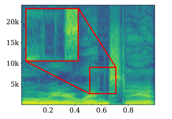
(a)

(b)

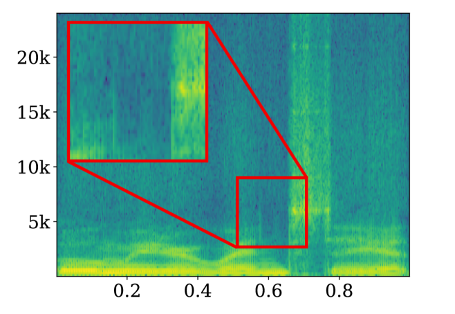
(c)

Fig. 3: Super resolution results in spectrogram. (a) Ground Truth is 48kHz signal, (b) and (c) are super resolution results of the $\times 4$ (12kHz $\to$ 48kHz) setting in Table 1.

Throughout the experiments, we use CSTR VCTK corpus [18], a high-quality speech dataset in 48kHz uttered by 109 English speakers. We inherit the same multi-speaker setting used in [7], where the first 99 speakers are used for training and the rest are served as test set. We compare our method with the existing audio super resolution methods including AudioUNet [7], AudioTFilm [19], and WSRGlow [10]. To be as fair as possible, we use the pre-trained models of baselines if available, and we reproduce using the original authors’ official source codes otherwise. We evaluate the performance of super resolution in terms of Signal-to-Noise-Ratio (SNR) and Log-Spectral-Distance (LSD). SNR is defined as

$$\text{SNR}({\mathbf{x}},\hat{\mathbf{x}})=10\log\frac{\|{\mathbf{x}}\|_{2}^{2}}{\|{\mathbf{x}}-\hat{\mathbf{x}}\|_{2}^{2}}\;,$$ (4)

where $\hat{x}$ is the predicted signal and $x$ is the ground truth signal. LSD is defined as

$$\text{LSD}({\mathbf{x}},\hat{\mathbf{x}})=\frac{1}{L}\sum_{l=1}^{L}\sqrt{\frac{1}{K}\sum_{k=1}^{K}\left(X(l,k)-\hat{X}(l,k)\right)^{2}}\;,$$ (5)

where, using Short-Time Fourier Transform (STFT), $X(l,k)=\log|\text{STFT}^{(l,k)}({\mathbf{x}})|^{2}$ is log-spectral power magnitudes of ${\mathbf{x}}$ with index frame $l$ and frequency $k$, and $\hat{X}$ is defined similarly but for $\hat{\mathbf{x}}$. We use Adam optimizer [20] with learning rate of 0.001. We train the model for 50 epochs, and decay the learning rate by half at every 5 epochs. We use gradient clipping with $0.001$ max norm for stable training.

3.1 Fixed scale super resolution

Table 1: Objective comparison with other methods.

	$\times 2$ (24k$\to$48k)		$\times$4 (12k$\to$48k)		# params
	SNR$\uparrow$	LSD$\downarrow$	SNR$\uparrow$	LSD$\downarrow$
AudioUNet [7]	21.68	1.31	18.55	2.11	71M
AudioTFilm [19]	22.23	1.05	19.51	2.02	68M
WSRGlow [10]	25.29	0.61	19.41	1.01	229M
LISA (Ours)	30.7	0.58	24.16	0.81	89k

We train our model, LISA, on two tasks of fixed scale resolution: i) from 12kHz to 48kHz; and ii) from 24kHz to 48kHz. Table 1 compares LISA to the baselines, in which LISA shows the best performance in terms of both SNR and LSD. It is remarkable that in terms of the number of model parameters, our model is at least 764 times lighter than the others. In Fig 3, LISA captures detailed features in the spectrogram, which are highlighted with red boxes. However, WSRGlow misses the details despite it uses 2,573 times more parameters. The difference is noticeable in listening.

3.2 Arbitrary scale super resolution

Table 2: Evaluation of arbitrary scale super resolution and ablation study. The same model is used for 2$\times$, 3$\times$, and 6$\times$ super resolution. -sto, -spec denotes models trained without stochastic selection and without multi-scale spectrogram loss.

in-distribution out-of-distribution $\times$2 (8k$\to$16k) $\times$3 (8k$\to$24k) $\times$6 (8k$\to$48k) SNR$\uparrow$ LSD$\downarrow$ SNR$\uparrow$ LSD$\downarrow$ SNR$\uparrow$ LSD$\downarrow$ LISA 25.66 0.94 24.15 1.17 22.17 1.23 LISA (-sto) -0.18 +0.01 -0.05 +0.00 -0.04 +0.01 LISA (-spec) -0.08 +0.00 -0.07 +0.00 -0.04 +0.01

To demonstrate the arbitrary scale super resolution using LISA, we obtain a single model with the self-supervised learning tasks from $R_{\text{in}}=8\text{kHz}$ to the random target resolution drawn from $[R^{-}_{\text{out}},R^{+}_{\text{out}}]=[8\text{kHz},24\text{kHz}]$, i.e., the training never uses any sound of 48 kHz resolution.

Out-of-distribution. In Table 2, the model is evaluated with 2$\times$, 3$\times$, and 6$\times$ super resolution tasks. In the out-of-distribution task, which our model upsamples with a scale of 6, our model even outperforms the results of 4x super resolution task of baselines. Note that the 48kHz data, which is the output resolution of 6$\times$ setting, is never seen to the model while training.

Fig. 4: Super resolution performances at different scales.

Non-integer scale SR. Also, we evaluated our results in non-integer scale. In Fig 4, non-integer scale super resolution performance is no worse than integer scale super resolution, does not show any fluctuation. The test data is generated with sinc interpolation from 48k data.

Ablation Study. In Table 2, we also assess the effect of each component through an ablation study. The perturbed prediction (2.2.2) in training is twice beneficial in terms of SNR gain compared to the spectrogram loss function in (3) in the 2$\times$ super resolution. In addition, Fig 2 shows that the discontinuity between the local signals is indeed regulated by the perturbed prediction (2.2.2).

4 Conclusion

We propose LISA to obtain a continuous representation of an audio as a neural function, which enables us to perform the arbitrary scale audio super resolution. To train LISA, we devise a sophisticated self-supervised learning strategy, equipped with the perturbed prediction in training and the loss function for audio signal. Our experiment shows that LISA outperforms the other baselines in terms of super resolution performance with a remarkably small size. We expect that our model has a great potential for online audio super resolution applications thanks to the light size compared to other baseline models but also the low latency from the local implicit representation.

References

- [1] Gennaro Evangelista, “Design of digital systems for arbitrary sampling rate conversion,” Signal processing, vol. 83, no. 2, pp. 377–387, 2003.
- [2] Alan V. Oppenheim, Ronald W. Schafer, and John R. Buck, Discrete-Time Signal Processing, Prentice-hall Englewood Cliffs, second edition, 1999.
- [3] Xiaojing Huang, Y. Jay Guo, and Jian Andrew Zhang, “Sample rate conversion using b-spline interpolation for ofdm based software defined radios,” IEEE Transactions on Communications, vol. 60, no. 8, pp. 2113–2122, 2012.
- [4] Hannu Pulakka, Ulpu Remes, Kalle Palomäki, Mikko Kurimo, and Paavo Alku, “Speech bandwidth extension using gaussian mixture model-based estimation of the highband mel spectrum,” in ICASSP, 2011.
- [5] P. Jax and P. Vary, “Artificial bandwidth extension of speech signals using mmse estimation based on a hidden markov model,” in ICASSP, 2003.
- [6] Pramod Bachhav, Massimiliano Todisco, and Nicholas Evans, “Efficient super-wide bandwidth extension using linear prediction based analysis-synthesis,” in ICASSP, 2018.
- [7] Volodymyr Kuleshov, S Zayd Enam, and Stefano Ermon, “Audio super resolution using neural networks,” arXiv:1708.00853, 2017.
- [8] S. E. Eskimez, K. Koishida, and Z. Duan, “Adversarial training for speech super-resolution,” IEEE Journal of Selected Topics in Signal Processing, vol. 13, no. 2, pp. 347–358, 2019.
- [9] Jiaqi Su, Yunyun Wang, Adam Finkelstein, and Zeyu Jin, “Bandwidth extension is all you need,” in ICASSP, 2021.
- [10] Kexun Zhang, Yi Ren, Changliang Xu, and Zhou Zhao, “Wsrglow: A glow-based waveform generative model for audio super-resolution,” in INTERSPEECH, 2021.
- [11] Vincent Sitzmann, Julien N.P. Martel, Alexander W. Bergman, David B. Lindell, and Gordon Wetzstein, “Implicit neural representations with periodic activation functions,” in NeurIPS, 2020.
- [12] Jeong Joon Park, Peter Florence, Julian Straub, Richard Newcombe, and Steven Lovegrove, “Deepsdf: Learning continuous signed distance functions for shape representation,” in CVPR, 2019.
- [13] Ben Mildenhall, Pratul P Srinivasan, Matthew Tancik, Jonathan T Barron, Ravi Ramamoorthi, and Ren Ng, “Nerf: Representing scenes as neural radiance fields for view synthesis,” in ECCV, 2020.
- [14] Yinbo Chen, Sifei Liu, and Xiaolong Wang, “Learning continuous image representation with local implicit image function,” in CVPR, 2021.
- [15] Ishit Mehta, Michaël Gharbi, Connelly Barnes, Eli Shechtman, Ravi Ramamoorthi, and Manmohan Chandraker, “Modulated periodic activations for generalizable local functional representations,” arXiv:2104.03960, 2021.
- [16] C.E. Shannon, “Communication in the presence of noise,” Proceedings of the IRE, vol. 37, no. 1, pp. 10–21, 1949.
- [17] Ryuichi Yamamoto, Eunwoo Song, and Jae-Min Kim, “Parallel wavegan: A fast waveform generation model based on generative adversarial networks with multi-resolution spectrogram,” in ICASSP, 2020.
- [18] Christophe Veaux, Junichi Yamagishi, and Kirsten MacDonald, “CSTR VCTK Corpus: English multi-speaker corpus for cstr voice cloning toolkit,” 2016.
- [19] Sawyer Birnbaum, Volodymyr Kuleshov, S. Zayd Enam, Pang Wei Koh, and Stefano Ermon, “Temporal film: Capturing long-range sequence dependencies with feature-wise modulation,” in NeurIPS, 2019.
- [20] Diederik Kingma and Jimmy Ba, “Adam: A method for stochastic optimization,” in ICLR, 2015.