A Riemannian Inexact Newton Dogleg Method for Constructing a Symmetric Nonnegative Matrix with Prescribed Spectrum

Abstract

This paper is concerned with the inverse problem of constructing a symmetric nonnegative matrix from realizable spectrum. We reformulate the inverse problem as an underdetermined nonlinear matrix equation over a Riemannian product manifold. To solve it, we develop a Riemannian underdetermined inexact Newton dogleg method for solving a general underdetermined nonlinear equation defined between Riemannian manifolds and Euclidean spaces. The global and quadratic convergence of the proposed method is established under some mild assumptions. Then we solve the inverse problem by applying the proposed method to its equivalent nonlinear matrix equation and a preconditioner for the perturbed normal Riemannian Newton equation is also constructed. Numerical tests show the efficiency of the proposed method for solving the inverse problem.

Keywords. Symmetric nonnegative inverse eigenvalue problem, underdetermined equation, Riemannian Newton dogleg method, preconditioner.

AMS subject classifications. 15A18, 65F08, 65F18, 65F15.

1 Introduction

An $n$-by-$n$ matrix $A$ is nonnegative if all its entries are all nonnegative, i.e., $(A)_{ij}\geq 0$ for all $i,j=1,\ldots,n$, where $(A)_{ij}$ means the $(i,j)$th entry of $A$. Nonnegative matrices arise in a wide variety of applications such as finite Markov chains, probabilistic algorithms, graph theory, the linear complementarity problems, matrix scaling, and input-output analysis in economics, etc (see for instance [3, 4, 28, 34]). The nonnegative inverse eigenvalue problem (NIEP) is a structured inverse eigenvalue problem [9, 10, 40], which aims to determine whether a given self-conjugate set of complex numbers is the spectrum of a nonnegative matrix. Various theoretical results have been obtained on the existence theory of the NIEP in the literature [16, 20, 21, 22, 23, 25, 29, 33, 35, 36].

This paper is concerned with the symmetric NIEP of constructing a symmetric nonnegative matrix from a realizable spectrum numerically. Recall that a list of complex numbers which occurs as the spectrum of some nonnegative matrix is called a realizable spectrum [20]. The inverse eigenvalue problem of reconstruction of a real symmetric nonnegative matrix from a prescribed realizable spectrum can be stated as follows:

SNIEP. Given a realizable list of $n$ real numbers $\{\lambda_{1},\lambda_{2},\ldots,\lambda_{n}\}$, find an $n$-by-$n$ real symmetric nonnegative matrix $A$ such that its eigenvalues are $\lambda_{1},\lambda_{2},\ldots,\lambda_{n}$.

There exist some numerical methods for solving the NIEP including constructive methods [21, 31, 37], recursive methods [14, 24], isospectral gradient flow approaches [5, 7, 8, 11], alternating projection algorithm [30] and Riemannian inexact Newton method [41]. Constructive methods and recursive methods have special requirements on the realizable spectrum, and thus these methods are restricted to solving the NIEPs with additional constraints on the realizable spectrum. Isospectral gradient approaches and alternating projection algorithms can be used in the solution of medium-scale problems. The Riemannian inexact Newton method can be applied to solve large-scale problems, which depends heavily on how to solve the Riemannian Newton equation efficiently. This motivates us to find an effective preconditioner to improve the efficiency of the proposed Riemannian Newton method for solving large-scale SNIEPs.

In the past few decades, various numerical methods have been proposed for finding zeros of underdetermined nonlinear maps defined between Euclidean spaces (see for instance [2, 6, 12, 13, 17, 27, 38, 39]). However, to our knowledge, except for the Riemannian inexact Newton method proposed in [41], there exist few other effective numerical algorithms in the literature for finding the zeros of general underdetermined maps between a Riemannian manifold and a Euclidean space.

In this paper, based on the symmetric Schur decomposition, we reformulate the SNIEP as a problem of finding a solution of an underdetermined nonlinear matrix equation over a product Riemannian manifold. To solve it, we first develop a Riemannian inexact Newton dogleg method for solving a general underdetermined nonlinear equation over a Riemannian manifold. This is motivated by the three papers due to Pawlowski et al. [32], Simons [38], and Zhao et al. [41]. In [38], Simons provided an exact trust region method (i.e., underdetermined Newton dogleg method) for finding zeros of underdetermined nonlinear maps defined between Euclidean spaces. In [32], Pawlowski et al. presented inexact Newton dogleg methods for solving nonlinear equations defined on a Euclidean space. In [41], Zhao et al. gave a Riemannian inexact Newton method for constructing a nonnegative matrix with prescribed realizable spectrum. The global and quadratic convergence of the proposed method is established under some mild assumptions. Then we find a solution to the SNIEP by applying the proposed method to its corresponding underdetermined nonlinear matrix equation over a product Riemannian manifold. To further improve the efficiency, by exploring the structure property of the SNIEP, a preconditioning technique is presented, which can also be combined with the Riemannian inexact Newton method in [41] for solving the SNIEP. Finally, we report some numerical experiments to demonstrate that the proposed method with the constructed preconditioner can solve the SNIEP efficiently.

Throughout this paper, we use the following notation. The symbols $A^{T}$ and $A^{H}$ denote the transpose and conjugate transpose of a matrix $A$, respectively. $I_{n}$ denotes the identity matrix of order $n$. Let ${\mathbb{R}}^{n\times n}$ and $\mathbb{SR}^{n\times n}$ be the set of all $n$-by-$n$ real matrices and the set of all $n$-by-$n$ real symmetric matrices, respectively. Let ${\mathbb{R}}^{n\times n}_{+}$ and $\mathbb{SR}^{n\times n}_{+}$ denote the nonnegative orthants of ${\mathbb{R}}^{n\times n}$ and $\mathbb{SR}^{n\times n}$, respectively. $\|\cdot\|_{F}$ stands for the matrix Frobenius norm. Denote by $A\odot B$ and $[A,B]:=AB-BA$ the Hadamard product and Lie Bracket of two $n$-by-$n$ matrices $A$ and $B$, respectively. Denote by ${\rm tr}(A)$ the sum of the diagonal entries of a square matrix $A$. ${\rm diag}({\bf a})$ is a diagonal matrix whose $i$th diagonal element is the $i$th component of a vector ${\bf a}$. For a matrix $A\in{\mathbb{R}}^{n\times n}$, let ${\rm vec}(A)$ be the vectorization of $A$, i.e., a column vector obtained by stacking the columns of $A$ on top of one another, and define ${\rm vech}(A)\in\mathbb{R}^{n(n+1)/2}$ by

$$\big{(}{\rm vech}(A)\big{)}_{{\frac{(j-1)j}{2}+i}}:=(A)_{ij},\quad 1\leq i\leq j\leq n.$$

Let $\mathcal{X}$ and $\mathcal{Y}$ be two finite-dimensional vector spaces equipped with a scalar inner product $\langle\cdot,\cdot\rangle$ and its induced norm $\|\cdot\|$. Let $\mathcal{A}:\mathcal{X}\to\mathcal{Y}$ be a linear operator such that $\mathcal{A}[x]\in\mathcal{Y}$ for all $x\in\mathcal{X}$, and the adjoint of $\mathcal{A}$ is denoted by $\mathcal{A}^{*}$. Define the operator norm of $\mathcal{A}$ by ${|\kern-1.07639pt|\kern-1.07639pt|\mathcal{A}|\kern-1.07639pt|\kern-1.07639pt|}:=\sup\{\|\mathcal{A}[x]\|\ |\ x\in\mathcal{X}\mbox{ with }\|x\|=1\}.$

The rest of this paper is organized as follows. In Section 2 the SNIEP is written as an underdetermined nonlinear matrix equation over a Riemannian product manifold. In Section 3 we develop a Riemannian inexact Newton dogleg method for solving a general underdetermined nonlinear equation over a Riemannian manifold. The global and quadratic convergence of the proposed method is established under some mild assumptions. In Section 4 we apply the Riemannian inexact Newton dogleg method developed in Section 3 to the SNIEP, where an effective preconditioner is also provided. Finally, some numerical experiments and concluding remarks are given in Sections 5 and 6, respectively.

2 Reformulation

In this section, we reformulate the SNIEP as an equivalent problem of solving a specific underdetermined nonlinear matrix equation over a Riemannian product manifold. Let $\Lambda$ be the diagonal matrix defined by

$$\Lambda:={\rm diag}(\boldsymbol{\lambda})\in{\mathbb{R}}^{n\times n},\quad\boldsymbol{\lambda}:=(\lambda_{1},\lambda_{2},\ldots,\lambda_{n})^{T}\in{\mathbb{R}}^{n}.$$

Define the orthogonal group $\mathcal{O}(n)$ by

$$\mathcal{O}(n):=\big{\{}Q\in\mathbb{R}^{n\times n}\ |\ Q^{T}Q=I_{n}\big{\}}.$$

The set $\mathbb{SR}^{n\times n}_{+}$ can be represented by

$$\mathbb{SR}^{n\times n}_{+}=\{S\odot S\in{\mathbb{R}}^{n\times n}\;|\;S\in\mathbb{SR}^{n\times n}\}.$$

Based on the symmetric Schur decomposition [18], the smooth manifold of isospectral matrices for $\mathbb{SR}^{n\times n}$ is given by

$$\mathcal{M}(\Lambda):=\{A=Q\Lambda Q^{T}\in\mathbb{SR}^{n\times n}\;|\;Q\in\mathcal{O}(n)\}.$$

Hence, the SNIEP has a solution if and only if $\mathcal{M}(\Lambda)\cap\mathbb{SR}^{n\times n}_{+}\neq\emptyset$.

Suppose the SNIEP has at least one solution. Then the SNIEP is reduced to the following constrained matrix equation:

$$\begin{array}[]{c}\Phi(S,Q):=S\odot S-Q\Lambda Q^{T}=\mathbf{0}_{n\times n},\quad\mbox{s.t. $(S,Q)\in\mathbb{SR}^{n\times n}\times\mathcal{O}(n)$},\end{array}$$ (2.1)

where $\mathbf{0}_{n\times n}$ means the zero matrix of order $n$.

We note that if $(\overline{S},\overline{Q})\in\mathbb{SR}^{n\times n}\times\mathcal{O}(n)$ is a solution to (2.1), then $\overline{C}:=\overline{S}\odot\overline{S}$ is a solution to the SNIEP. To avoid confusion, we refer to (2.1) as the SNIEP.

We point out that $\Phi:\mathbb{SR}^{n\times n}\times\mathcal{O}(n)\to\mathbb{SR}^{n\times n}$ is a smooth mapping from the product manifold $\mathbb{SR}^{n\times n}\times\mathcal{O}(n)$ to the Euclidean space $\mathbb{SR}^{n\times n}$. It is obvious that the dimension of $\mathbb{SR}^{n\times n}\times\mathcal{O}(n)$ is larger than the dimension of $\mathbb{SR}^{n\times n}$ for $n\geq 2$. This shows that the matrix equation $\Phi(S,Q)=\mathbf{0}_{n\times n}$ defined by (2.1) is underdetermined for $n\geq 2$.

3 General underdetermined nonlinear equation over Riemannian manifold

In this section, we consider a general underdetermined nonlinear equation, where the nonlinear map is a differentiable mapping between a Riemannian manifold and a Euclidean space. Then we introduce a Riemannian inexact Newton dogleg method for solving the underdetermined nonlinear equation. The global and quadratic convergence is also established under some mild assumptions.

3.1 Problem statement

Let $\mathcal{M}$ and $\mathcal{E}$ be respectively a Riemannian manifold and a Euclidean space with ${\rm dim}(\mathcal{M})>{\rm dim}(\mathcal{E})$. Let $F:\mathcal{M}\to\mathcal{E}$ be a differentiable nonlinear mapping between $\mathcal{M}$ and $\mathcal{E}$. In this subsection, we focus on the following underdetermined nonlinear equation:

$$F(x)=0,\qquad\text{subject to (s.t.)}\;x\in\mathcal{M},$$ (3.1)

where $0$ is the zero vector of $\mathcal{E}$.

For simplicity, let $\langle\cdot,\cdot\rangle$ denote the Riemannian metric on $\mathcal{M}$ and the inner product on $\mathcal{E}$ with its induced norm $\|\cdot\|$. Denote by $T_{x}\mathcal{M}$ the tangent space of $\mathcal{M}$ at a point $x\in\mathcal{M}$. Let ${\mathrm{D}}F(x):T_{x}\mathcal{M}\to T_{F(x)}\mathcal{E}\simeq\mathcal{E}$ be the differential (derivative) of $F$ at $x\in\mathcal{M}$ [1, p.38], where “$\simeq$” means the identification of two sets. Then a point $x\in\mathcal{M}$ is called a stationary point of $F$ if

$$\|F(x)\|\leq\|F(x)+{\mathrm{D}}F(x)[\Delta x]\|,\quad\forall\Delta x\in T_{x}\mathcal{M}.$$

Define the merit function $f:\mathcal{M}\to{\mathbb{R}}$ by

$$f(x):=\frac{1}{2}\|F(x)\|^{2},\quad\forall x\in\mathcal{M}.$$ (3.2)

By hypothesis, $F$ is differentiable. Then the function $f:\mathcal{M}\to{\mathbb{R}}$ is also differentiable. As in [1, p. 46], the Riemannian gradient ${\rm grad\;}f(x)$ of $f$ at $x\in\mathcal{M}$ is defined as the unique element in $T_{x}\mathcal{M}$ such that

$$\langle{\rm grad\;}f(x),\xi_{x}\rangle={\mathrm{D}}f(x)[\xi_{x}],\quad\forall\xi_{x}\in T_{x}\mathcal{M}.$$

If follows from (3.2) that the Riemannian gradient of $f$ at $x\in\mathcal{M}$ is give by [1, p.185]:

$${\rm grad\;}f(x)=({\mathrm{D}}F(x))^{*}[F(x)],$$ (3.3)

where $({\mathrm{D}}F(x))^{*}:T_{F(x)}\mathcal{E}\to T_{x}\mathcal{M}$ is the adjoint operator of ${\mathrm{D}}F(x)$. Specially, $x\in\mathcal{M}$ is a stationary point of $F$ if and only if $x\in\mathcal{M}$ is a stationary point of $f$, i.e., ${\rm grad\;}f(x)=({\mathrm{D}}F(x))^{*}[F(x)]=0_{x}$, where $0_{x}$ is the zero tangent vector of $T_{x}\mathcal{M}$.

3.2 Riemannian inexact Newton dogleg method

In the following, we develop a Riemannian trust region method for solving (3.1). Let $R$ be a retraction on $\mathcal{M}$ [1, p.55]. As in [32, 38], given the current point $x_{k}\in\mathcal{M}$, we consider the following linear model of the nonlinear map $F$ at $x_{k}\in\mathcal{M}$:

$$F(x_{k})+{\mathrm{D}}F(x_{k})[\xi_{k}],\qquad\;\xi_{k}\in T_{x_{k}}\mathcal{M}.$$ (3.4)

Let $\Delta x_{k}\in T_{x_{k}}\mathcal{M}$ be an exact or approximate minimizer of the following trust region least square problem:

$$\min_{\xi_{k}\in T_{x_{k}}\mathcal{M},\;\|\xi_{k}\|\leq\delta_{k}}\|F(x_{k})+{\mathrm{D}}F(x_{k})[\xi_{k}]\|,$$ (3.5)

where $\delta_{k}>0$ is the trust region radius. The actual reduction and predicted reduction induced by $\Delta x_{k}$ at the current point $x_{k}\in\mathcal{M}$ are defined by

$${\rm Ared}_{k}(\Delta x_{k}):=\|F(x_{k})\|-\|F(R_{x_{k}}(\Delta x_{k}))\|$$ (3.6)

and

$${\rm Pred}_{k}(\Delta x_{k}):=\|F(x_{k})\|-\|F(x_{k})+{\mathrm{D}}F(x_{k})[\Delta x_{k}]\|.$$ (3.7)

Then the Ared/Pred condition needs to be tested, i.e., whether $\Delta x_{k}$ satisfies the following condition

$$\frac{{\rm Ared}_{k}(\Delta x_{k})}{{\rm Pred}_{k}(\Delta x_{k})}=\frac{\|F(x_{k})\|-\|F(R_{x_{k}}(\Delta x_{k}))\|}{\|F(x_{k})\|-\|F(x_{k})+{\mathrm{D}}F(x_{k})[\Delta x_{k}]\|}\geq t,$$ (3.8)

where $0<t<1$ is given constant. If the Ared/Pred condition is satisfied by $\Delta x_{k}$, then define $x_{k+1}:=R_{x_{k}}(\Delta x_{k})$ and compute $\delta_{k+1}$ by a prescribed rule. If not, the trust region radius $\delta_{k}$ is shrunk and we need find a new tangent vector $\Delta x_{k}\in T_{x_{k}}\mathcal{M}$ within the trust region.

We note that the nonlinear equation $F(x)=0$ is underdetermined. Hence, the global minimizer of (3.5) is not unique. To calculate a suitable $\Delta x_{k}\in T_{x_{k}}\mathcal{M}$, we can generalize the idea of exact trust region method for solving underdetermined equation between Euclidean spaces [38, p.34] in the following way

$$\Delta x_{k}:=\operatorname*{argmin}_{\xi_{k}\bot{\rm null}({\mathrm{D}}F(x_{k})),\;\|\xi_{k}\|\leq\delta_{k}}\|F(x_{k})+{\mathrm{D}}F(x_{k})[\xi_{k}]\|,$$ (3.9)

where ${\rm null}(\cdot)$ means the null space of a linear mapping. In general, the computation of $\Delta x_{k}$ by (3.9) is costly for large-scale problems.

In this paper, we generalize the underdetermined dogleg method in [38, p.42], which was presented for solving an underdetermined nonlinear equation defined between Euclidean spaces, to the solution of (3.1) over $\mathcal{M}$. Suppose that ${\rm grad\;}f(x_{k})\neq 0_{x_{k}}$, the Cauchy point at $x_{k}\in\mathcal{M}$ is defined to be the minimizer of $\frac{1}{2}\|F(x_{k})+{\mathrm{D}}F(x_{k})[\Delta x_{k}]\|^{2}$ along the steepest descent direction $-{\rm grad\;}f(x_{k})=-({\mathrm{D}}F(x))^{*}[F(x)]$, which is denoted by $\Delta x_{k}^{CP}$, i.e.,

$$\Delta x_{k}^{CP}:=-\frac{\|({\mathrm{D}}F(x_{k}))^{*}[F(x_{k})]\|^{2}}{\|{\mathrm{D}}F(x_{k})\circ({\mathrm{D}}F(x_{k}))^{*}[F(x_{k})]\|^{2}}({\mathrm{D}}F(x_{k}))^{*}[F(x_{k})]\in T_{x_{k}}\mathcal{M}.$$ (3.10)

Specially, we have

$$\Delta x_{k}^{CP}\perp{\rm null}({\mathrm{D}}F(x_{k})).$$ (3.11)

The Riemannian Newton point $\Delta x_{k}^{N}$ is defined by

$$\begin{array}[]{cc}\Delta x_{k}^{N}:=\operatorname*{argmin}\limits_{\xi_{k}\perp{\rm null}({\mathrm{D}}F(x_{k}))}\|F(x_{k})+{\mathrm{D}}F(x_{k})[\xi_{k}]\|\in T_{x_{k}}\mathcal{M}.\end{array}$$ (3.12)

The dogleg curve $\Gamma^{DL}_{k}$ is defined to be the piecewise linear curve joining the origin $0_{x_{k}}$, the Cauchy point $\Delta x_{k}^{CP}$, and the Riemannian Newton point $\Delta x_{k}^{N}$. Similar to the analysis in [38, pp. 42-44], the norm of the linear model $F(x_{k})+{\mathrm{D}}F(x_{k})[\xi_{x_{k}}]$ is monotone decreasing along the dogleg $\Gamma^{DL}_{k}$. By (3.11) and (3.12) we have

$$\Delta x_{k}\perp{\rm null}({\mathrm{D}}F(x_{k})),\quad\forall\Delta x_{k}\in\Gamma^{DL}_{k}.$$ (3.13)

The Riemannian dogleg step aims to find the tangent vector $\Delta x_{k}$ such that

$$\Delta x_{k}:=\operatorname*{argmin}_{\xi_{k}\in\Gamma^{DL}_{k},\;\|\xi_{k}\|\leq\delta_{k}}\|F(x_{k})+{\mathrm{D}}F(x_{k})[\xi_{k}]\|.$$

The above minimization problem has a unique minimizer, which can be calculated explicitly. The dogleg method is a special inexact trust region method, which is often computationally efficient than the exact trust region method. However, the Newton point $\Delta x_{k}^{N}$ is still computationally costly for large-scale problems. Based on (3.9), (3.13), and the analysis in [38], the orthogonality of $\Delta x_{k}$ with the null space of ${\mathrm{D}}F(x_{k})$ is essential for the convergence analysis.

In [32], inexact Newton dogleg methods were given for solving nonlinear equations defined on Euclidean spaces. To generalize these methods directly to the solution of (3.1), we need to find an inexact Newton point $\Delta x_{k}^{IN}\in T_{x_{k}}\mathcal{M}$ such that

$$\frac{\|F(x_{k})+{\mathrm{D}}F(x_{k})[\Delta x_{k}^{IN}]\|}{\|F(x_{k})\|}<\eta_{k}<\eta_{\max}<1\quad\mbox{and}\quad\Delta x_{k}^{IN}\perp{\rm null}({\mathrm{D}}F(x_{k})),$$ (3.14)

where $\eta_{k}$ is a forcing term [15]. However, if the differential ${\mathrm{D}}F(x_{k}):T_{x_{k}}\mathcal{M}\to T_{F(x_{k})}\mathcal{E}$ is not surjective, the first condition in (3.14) may not be attainable. The Riemannian Newton point $T_{x_{k}}\mathcal{M}\ni\Delta x_{k}^{N}\perp{\rm null}({\mathrm{D}}F(x_{k}))$ defined by (3.12) is the minimum norm solution of the least squares problem

$$\min\limits_{\Delta x_{k}\in T_{x_{k}}\mathcal{M}}\|F(x_{k})+{\mathrm{D}}F(x_{k})[\Delta x_{k}^{N}]\|,$$

which is given in the form of

$$\Delta x_{k}^{N}=-({\mathrm{D}}F(x_{k}))^{\dagger}F(x_{k}),$$

where $({\mathrm{D}}F(x_{k}))^{\dagger}$ denotes the pseudoinverse of the linear operator ${\mathrm{D}}F(x_{k})$ [26, pp. 163–164]. We note that

$$({\mathrm{D}}F(x_{k}))^{\dagger}=\lim_{\sigma\to 0^{+}}({\mathrm{D}}F(x_{k}))^{*}\circ\big{(}{\mathrm{D}}F(x_{k})\circ({\mathrm{D}}F(x_{k}))^{*}+\sigma\mathrm{id}_{T_{F(x_{k})}\mathcal{E}}\big{)}^{-1},$$

where $\mathrm{id}_{T_{F(x_{k})}\mathcal{E}}$ is the identity operator on $T_{F(x_{k})}\mathcal{E}$. This motivates us to solve the following perturbed Riemannian normal equation

$$\Big{(}{\mathrm{D}}F(x_{k})\circ({\mathrm{D}}F(x_{k}))^{*}+\sigma_{k}\mathrm{id}_{T_{F(x_{k})}\mathcal{E}}\Big{)}[\Delta z_{k}]=-F(x_{k}),$$ (3.15)

for $\Delta z_{k}\in T_{F(x_{k})}\mathcal{E}$, where $\sigma_{k}>0$ is a given constant. We observe that

$${\mathrm{D}}F(x_{k})\circ({\mathrm{D}}F(x_{k}))^{*}+\sigma_{k}\mathrm{id}_{T_{F(x_{k})}\mathcal{E}}$$

is a self-adjoint positive definite linear operator defined on the Euclidean space $\mathcal{E}$. Therefore, we can solve (3.15) inexactly by using the conjugate gradient (CG) method [18]. Moreover, once an approximate solution $\Delta z_{k}$ is obtained, the inexact Newton point is given by $\Delta x_{k}^{IN}:=({\mathrm{D}}F(x_{k}))^{*}[\Delta z_{k}]$, which satisfies the second condition in (3.14) naturally.

Therefore, the inexact dogleg curve $\widehat{\Gamma}^{DL}_{k}$ is defined to be the piecewise linear curve joining the origin $0_{x_{k}}$, the Cauchy point $\widehat{\Delta x}_{k}^{CP}$ defined by

$$\widehat{\Delta x}_{k}^{CP}:=-\frac{\|({\mathrm{D}}F(x_{k}))^{*}[F(x_{k})]\|^{2}}{\|{\mathrm{D}}F(x_{k})\circ({\mathrm{D}}F(x_{k}))^{*}[F(x_{k})]\|^{2}}({\mathrm{D}}F(x_{k}))^{*}[F(x_{k})],$$ (3.16)

and the Riemannian inexact Newton point $\Delta x_{k}^{IN}$.

Based on the above analysis and sparked by the ideas in [32, 38, 41], we propose the following Riemannian inexact Newton dogleg method for solving (3.1).

(Riemannian inexact Newton dogleg method)

Step 0.

Choose an initial point $x_{0}\in\mathcal{M}$, $\epsilon>0$, $0<t<1$, $0<\sigma_{\max}<1$, $0<\theta_{\max}<1$, $0<\delta_{\min}<1$, $\delta_{0}\geq\delta_{\min}$, and a nonnegative sequences $\{\bar{\eta}_{k}\in(0,1)\}$ with $\lim_{k\to\infty}\bar{\eta}_{k}=0$. Let $k:=0$.

Step 1.

If $\|F(x_{k})\|<\epsilon$, then stop.

Step 2.

Apply the CG method to solve (3.15) for $\Delta z_{k}\in T_{F(x_{k})}\mathcal{E}$ such that

$$\begin{array}[]{l}\big{\|}\big{(}{\mathrm{D}}F(x_{k})\circ({\mathrm{D}}F(x_{k}))^{*}+\sigma_{k}\mathrm{id}_{T_{F(x_{k})}\mathcal{E}}\big{)}[\Delta z_{k}]+F(x_{k})\big{\|}\leq\eta_{k}\|F(x_{k})\|\end{array}$$ (3.17)

and

$$\begin{array}[]{l}\|{\mathrm{D}}F(x_{k})\circ({\mathrm{D}}F(x_{k}))^{*}[\Delta z_{k}]+F(x_{k})\|<\|F(x_{k})\|,\end{array}$$ (3.18)

where

$$\sigma_{k}:=\min\{\sigma_{\max},\|F(x_{k})\|\}\quad\mbox{and}\quad\eta_{k}:=\min\{\bar{\eta}_{k},\|F(x_{k})\|\}.$$ (3.19)

Step 3.

Define

$$\Delta x_{k}^{IN}:=({\mathrm{D}}F(x_{k}))^{*}[\Delta z_{k}].$$ (3.20)

Compute $\widehat{\Delta x}_{k}^{CP}$ by (3.16). Determine $\Delta x_{k}\in\widehat{\Gamma}^{DL}_{k}$ with $\min\{\delta_{\min},\|\Delta x_{k}^{IN}\|\}\leq\|\Delta x_{k}\|\leq\delta_{k}$.

Step 4.

While ${\rm Ared}_{k}(\Delta x_{k})<t\cdot{\rm{\rm{\rm Pred}}_{k}}(\Delta x_{k})$ do:
If $\delta_{k}=\delta_{\min}$, stop; else choose $\theta_{k}\in(0,\theta_{\max}]$.
Update $\delta_{k}=\max\{\theta_{k}\delta_{k},\delta_{\min}\}$.
Redetermine $\Delta x_{k}\in\widehat{\Gamma}^{DL}_{k}$ with $\min\{\delta_{\min},\|\Delta x_{k}^{IN}\|\}\leq\|\Delta x_{k}\|\leq\delta_{k}$.

Step 5.

Set $x_{k+1}:=R_{x_{k}}(\Delta x_{k})$. Update $\delta_{k+1}\in[\delta_{\min},\infty)$.

Step 6.

Replace $k$ by $k+1$ and go to Step 1.

On Algorithm 3.2, we have several remarks as follows:

• The choices of $\sigma_{k}$ and $\eta_{k}$ in (3.19) are sparked by the similar idea in [41].

• The norm of the linear model $F(x_{k})+{\mathrm{D}}F(x_{k})[\xi_{x_{k}}]$ is monotone decreasing along the segment of the inexact dogleg curve $\widehat{\Gamma}_{k}^{DL}$ between $0_{x_{k}}$ and $\widehat{\Delta x}_{k}^{CP}$, while it may not be monotone decreasing along the segment of $\widehat{\Gamma}_{k}^{DL}$ between $\widehat{\Delta x}_{k}^{CP}$ and $\Delta x_{k}^{IN}$.

• We observe from Step 4 of Algorithm 3.2, (3.6), and (3.7) that for all $k\geq 0$,

  $$\|F(x_{k})\|-\|F(x_{k+1})\|\geq t(\|F(x_{k})\|-\|F(x_{k})+{\mathrm{D}}F(x_{k})[\Delta x_{k}]\|).$$ (3.21)

  This shows that the sequence $\{F(x_{k})\}$ is monotone decreasing if Algorithm 3.2 does not break down.

• The procedure for determining $\Delta x_{k}$ and $\delta_{k+1}$ in Steps 3–5 of Algorithm 3.2 is presented in Section 5.

3.3 Convergence analysis

In this subsection, we establish the global and quadratic convergence of Algorithm 3.2. Let

$$\Omega:=\big{\{}x\in\mathcal{M}\ |\ \|F(x)\|\leq\|F(x_{0})\|\big{\}}.$$ (3.22)

To derive the global convergence of Algorithm 3.2, we need the following basic assumption.

Assumption 3.1

1. The mapping $F:\mathcal{M}\to\mathcal{E}$ is continuously differentiable on the level set $\Omega$.

2. For the retraction $R$ defined on $\mathcal{M}$, there exist two scalars $\nu>0$ and $\mu_{\nu}>0$ such that

   $$\nu\|\Delta x\|\geq{\rm dist}\big{(}x,R_{x}(\Delta x)\big{)},$$

   for all $x\in\Omega$ and $\Delta x\in T_{x}\mathcal{M}$ with $\|\Delta x\|\leq\mu_{\nu}$, where “dist” means the Riemannian distance on $\mathcal{M}$.

Remark 3.2

If the level set $\Omega$ is compact, then the second condition in Assumption 3.1 is satisfied. This is guaranteed if the Riemannian manifold $\mathcal{M}$ is compact [1, p. 149].

To show the convergence of Algorithm 3.2, for the iterates $\Delta x_{k}^{IN}$, $\widehat{\Delta x}_{k}^{CP}$, and $\Delta x_{k}$ generated by Algorithm 3.2, define

$$\eta^{IN}_{k}:=\frac{\|F(x_{k})+{\mathrm{D}}F(x_{k})[\Delta x_{k}^{IN}]\|}{\|F(x_{k})\|},$$ (3.23)

$$\eta_{k}^{CP}:=\frac{\|F(x_{k})+{\mathrm{D}}F(x_{k})[\widehat{\Delta x}_{k}^{CP}]\|}{\|F(x_{k})\|},$$ (3.24)

$$\tau_{k}:=\frac{\|F(x_{k})+{\mathrm{D}}F(x_{k})[\Delta x_{k}]\|}{\|F(x_{k})\|}\equiv 1-\frac{{\rm Pred}_{k}(\Delta x_{k})}{\|F(x_{k})\|}.$$ (3.25)

In the following, we give some lemmas, which are necessary for deducing the global convergence of Algorithm 3.2. First, by following the similar arguments of [41, Lemma 1], we have the following result on the reachability of conditions (3.17) and (3.18) for solving (3.15).

Lemma 3.3

Let $x_{k}$ be the current iterate generated by Algorithm 3.2. If ${\rm grad\;}f(x_{k})\neq 0_{x_{k}}$, then we can solve (3.15) sufficiently accurately such that (3.17) and (3.18) are satisfied.

On the quantity $\eta^{IN}_{k}$ defined by (3.23), we have the following lemma.

Lemma 3.4

Let $x_{k}$ be the current iterate generated by Algorithm 3.2. If ${\rm grad\;}f(x_{k})\neq 0_{x_{k}}$, then, for $\eta^{IN}_{k}$ defined by (3.23), we have

$$\eta^{IN}_{k}\leq\frac{\sigma_{k}}{\sigma_{k}+\lambda_{\min}\big{(}{\mathrm{D}}F(x_{k})\circ({\mathrm{D}}F(x_{k}))^{*}\big{)}}+\eta_{k}\quad\mbox{and}\quad\eta^{IN}_{k}<1,$$

where $\lambda_{\min}(\cdot)$ denotes the smallest eigenvalue of a linear operator.

Proof. This follows from Lemma 3.3 and [41, Lemma 3].

On the quantity $\eta_{k}^{CP}$ defined by (3.24), we have the following result.

Lemma 3.5

Let $x_{k}$ be the current iterate generated by Algorithm 3.2. If ${\rm grad\;}f(x_{k})\neq 0_{x_{k}}$, then, for $\eta_{k}^{CP}$ defined by (3.24), we have

$$\eta_{k}^{CP}<1.$$

Proof. By hypothesis, ${\rm grad\;}f(x_{k})=({\mathrm{D}}F(x_{k}))^{*}[F(x_{k})]\neq 0_{x_{k}}$. Thus,

$$0 < \|({\mathrm{D}}F(x_{k}))^{*}[F(x_{k})]\|^{2}=\langle({\mathrm{D}}F(x_{k}))^{*}[F(x_{k})],({\mathrm{D}}F(x_{k}))^{*}[F(x_{k})]\rangle$$ (3.26)

$$= \langle F(x_{k}),{\mathrm{D}}F(x_{k})\circ({\mathrm{D}}F(x_{k}))^{*}[F(x_{k})]\rangle$$

$$\leq \|F(x_{k})\|\cdot\|{\mathrm{D}}F(x_{k})\circ({\mathrm{D}}F(x_{k}))^{*}[F(x_{k})]\|.$$

It follows from (3.16) that

$$\|F(x_{k})+{\mathrm{D}}F(x_{k})[\widehat{\Delta x}_{k}^{CP}]\|^{2}$$

$$= \|F(x_{k})\|^{2}+\|{\mathrm{D}}F(x_{k})[\widehat{\Delta x}_{k}^{CP}]\|^{2}+2\langle F(x_{k}),{\mathrm{D}}F(x_{k})[\widehat{\Delta x}_{k}^{CP}]\rangle$$

$$= \|F(x_{k})\|^{2}+\frac{\|({\mathrm{D}}F(x_{k}))^{*}[F(x_{k})]\|^{4}}{\|{\mathrm{D}}F(x_{k})\circ({\mathrm{D}}F(x_{k}))^{*}[F(x_{k})]\|^{4}}\|{\mathrm{D}}F(x_{k})\circ({\mathrm{D}}F(x_{k}))^{*}[F(x_{k})]\|^{2}$$

$$-\frac{2\|({\mathrm{D}}F(x_{k}))^{*}[F(x_{k})]\|^{2}}{\|{\mathrm{D}}F(x_{k})\circ({\mathrm{D}}F(x_{k}))^{*}[F(x_{k})]\|^{2}}\langle F(x_{k}),{\mathrm{D}}F(x_{k})\circ({\mathrm{D}}F(x_{k}))^{*}[F(x_{k})]\rangle$$

$$= \|F(x_{k})\|^{2}-\frac{\|({\mathrm{D}}F(x_{k}))^{*}[F(x_{k})]\|^{4}}{\|{\mathrm{D}}F(x_{k})\circ({\mathrm{D}}F(x_{k}))^{*}[F(x_{k})]\|^{2}}$$

$$= \|F(x_{k})\|^{2}\Bigg{(}1-\frac{\|({\mathrm{D}}F(x_{k}))^{*}[F(x_{k})]\|^{4}}{\|F(x_{k})\|^{2}\|{\mathrm{D}}F(x_{k})\circ({\mathrm{D}}F(x_{k}))^{*}[F(x_{k})]\|^{2}}\Bigg{)}.$$

This, together with (3.24) and (3.26), yields $\eta_{k}^{CP}<1$.

On the quantity $\tau_{k}$ defined by (3.25), we have the following result.

Lemma 3.6

Let $x_{k}$ be the current iterate generated by Algorithm 3.2. If ${\rm grad\;}f(x_{k})\neq 0_{x_{k}}$, then, for $\tau_{k}$ defined by (3.25), we have

$$0\leq\tau_{k}<1,\quad\|F(x_{k+1})\|\leq(1-t(1-\tau_{k}))\|F(x_{k})\|.$$

Proof. By hypothesis, ${\rm grad\;}f(x_{k})=({\mathrm{D}}F(x_{k}))^{*}[F(x_{k})]\neq 0_{x_{k}}$, i.e., $x_{k}$ is not a stationary point of $f$. Since $\|F(x_{k})+{\mathrm{D}}F(x_{k})[\xi_{x_{k}}]\|$ is strictly monotone decreasing along the segment of $\widehat{\Gamma}_{k}^{DL}$ between $0_{x_{k}}$ and $\widehat{\Delta x}_{k}^{CP}$, if $\Delta x_{k}$ lies on $\widehat{\Gamma}^{DL}_{k}$ between $0_{x_{k}}$ and $\widehat{\Delta x}_{k}^{CP}$, we have

$$\eta_{k}^{CP}\|F(X_{k})\|\leq\|F(x_{k})+{\mathrm{D}}F(x_{k})[\Delta x_{k}]\|<\|F(x_{k})\|.$$ (3.27)

If $\Delta x_{k}$ lies on $\widehat{\Gamma}^{DL}_{k}$ between $\widehat{\Delta x}_{k}^{CP}$ and $\Delta x_{k}^{IN}$, then it follows from (3.23), (3.24), norm convexity, and Lemmas 3.4 and 3.5 that

$$0\leq\|F(x_{k})+{\mathrm{D}}F(x_{k})[\Delta x_{k}]\|\leq\max\{\eta_{k}^{CP},\eta_{k}^{IN}\}\|F(x_{k})\|<\|F(x_{k})\|.$$ (3.28)

Based on (3.25), (3.27), and (3.28), we can obtain $0\leq\tau_{k}<1$. Then, we have by (3.21),

$$\|F(x_{k+1})\|\leq\|F(x_{k})\|-t(\|F(x_{k})\|-\|F(x_{k})+{\mathrm{D}}F(x_{k})[\Delta x_{k}]\|)=\big{(}1-t(1-\tau_{k})\big{)}\|F(x_{k})\|,$$

This completes the proof.

On the iterate $\Delta x_{k}^{IN}$ generated by Algorithm 3.2, we have the following result.

Lemma 3.7

Let $x_{k}$ be the current iterate generated by Algorithm 3.2. If ${\rm grad\;}f(x_{k})\neq 0_{x_{k}}$, then

$$\|\Delta x_{k}^{IN}\|\leq(1+\eta_{k}){|\kern-1.07639pt|\kern-1.07639pt|({\mathrm{D}}F(x_{k}))^{\dagger}|\kern-1.07639pt|\kern-1.07639pt|}\cdot\|F(x_{k})\|.$$

Proof. It follows from the same arguments of [41, Lemma 2].

On the iterate $\widehat{\Delta x}_{k}^{CP}$ generated by Algorithm 3.2, we have the following result.

Lemma 3.8

Let $x_{k}$ be the current iterate generated by Algorithm 3.2. If ${\rm grad\;}f(x_{k})\neq 0_{x_{k}}$ and ${\mathrm{D}}F(x_{k})$ is surjective, then

$$\|\widehat{\Delta x}_{k}^{CP}\|\leq\lambda_{\min}^{-\frac{1}{2}}\big{(}{\mathrm{D}}F(x_{k})\circ({\mathrm{D}}F(x_{k}))^{*}\big{)}\|F(x_{k})\|.$$ (3.29)

Proof. By hypothesis, ${\rm grad\;}f(x_{k})=({\mathrm{D}}F(x_{k}))^{*}[F(x_{k})]\neq 0_{x_{k}}$. Since ${\mathrm{D}}F(x_{k})$ is surjective, we know that $\lambda_{\min}({\mathrm{D}}F(x_{k})\circ({\mathrm{D}}F(x_{k}))^{*})>0$. Using the definition of $\widehat{\Delta x}_{k}^{CP}$ we have

$$\Big{\|}\widehat{\Delta x}_{k}^{CP}\Big{\|} = \frac{\|({\mathrm{D}}F(x_{k}))^{*}[F(x_{k})]\|^{2}}{\|{\mathrm{D}}F(x_{k})\circ({\mathrm{D}}F(x_{k}))^{*}[F(x_{k})]\|^{2}}\|({\mathrm{D}}F(x_{k}))^{*}[F(x_{k})]\|$$

$$= \frac{\|({\mathrm{D}}F(x_{k}))^{*}[F(x_{k})]\|^{4}}{\|{\mathrm{D}}F(x_{k})\circ({\mathrm{D}}F(x_{k}))^{*}[F(x_{k})]\|^{2}}\cdot\frac{1}{\|({\mathrm{D}}F(x_{k}))^{*}[F(x_{k})]\|}$$

$$= \frac{\langle F(x_{k}),{\mathrm{D}}F(x_{k})\circ({\mathrm{D}}F(x_{k}))^{*}[F(x_{k})]\rangle^{2}}{\|{\mathrm{D}}F(x_{k})\circ({\mathrm{D}}F(x_{k}))^{*}[F(x_{k})]\|^{2}}\cdot\frac{1}{\|({\mathrm{D}}F(x_{k}))^{*}[F(x_{k})]\|}$$

$$\leq \frac{\|F(x_{k})\|^{2}}{\|({\mathrm{D}}F(x_{k}))^{*}[F(x_{k})]\|}=\left(\frac{\|F(x_{k})\|^{2}}{\langle(F(x_{k}),{\mathrm{D}}F(x_{k})\circ{\mathrm{D}}F(x_{k}))^{*}[F(x_{k})]\rangle}\right)^{\frac{1}{2}}\|F(x_{k})\|$$

$$\leq \lambda_{\min}^{-\frac{1}{2}}\big{(}{\mathrm{D}}F(x_{k})\circ({\mathrm{D}}F(x_{k}))^{*}\big{)}\|F(x_{k})\|.$$

We now derive the following result on the sequence $\{\eta^{IN}_{k}\}$ generated by Algorithm 3.2, where $\eta^{IN}_{k}$ is defined by (3.23).

Lemma 3.9

Suppose the first condition of Assumption 3.1 is satisfied and Algorithm 3.2 generates an infinite iterative sequence $\{x_{k}\}$. Let $\bar{x}$ be an accumulation point of $\{x_{k}\}$ and $\{x_{k}\}_{k\in\mathcal{K}}$ be a subsequence of $\{x_{k}\}$ converging to $\bar{x}$. If ${\rm grad\;}f(\bar{x})\neq 0_{\bar{x}}$, then, for $\eta^{IN}_{k}$ defined by (3.23), we have

$$\lim\limits_{k\to\infty,k\in\mathcal{K}}\eta_{k}^{IN}<1.$$

Proof. By hypothesis, ${\rm grad\;}f(\bar{x})=({\mathrm{D}}F(\bar{x}))^{*}[F(\bar{x})]\neq 0_{\bar{x}}$. Thus $F(\bar{x})\neq 0$. Since $\bar{x}$ is an accumulation point of $\{x_{k}\}$, there exists a subsequence $\{x_{k}\}_{k\in\mathcal{K}}$, which converges to $\bar{x}$. Hence, by the continuous differentiability of $F$, there exists a constant $c>0$ such that for all $k\in\mathcal{K}$ sufficiently large,

$$\|F(x_{k})\|\geq c.$$ (3.30)

This, together with (3.19), yields

$$\bar{\sigma}=\lim_{k\to\infty,\;k\in\mathcal{K}}\sigma_{k}\geq\min\{\sigma_{\max},c\}>0.$$ (3.31)

We note that $F$ is continuously differentiable. Thus,

$$\lim\limits_{k\to\infty,k\in\mathcal{K}}{\mathrm{D}}F(x_{k})={\mathrm{D}}F(\bar{x}),\quad\mbox{and}\quad\lim\limits_{k\to\infty,k\in\mathcal{K}}({\mathrm{D}}F(x_{k}))^{*}=({\mathrm{D}}F(\bar{x}))^{*}.$$ (3.32)

Let

$$W(x_{k}):=\big{(}{\mathrm{D}}F(x_{k})\circ({\mathrm{D}}F(x_{k}))^{*}+\sigma_{k}\mathrm{id}_{T_{F(x_{k})}\mathcal{E}}\big{)}[\Delta z_{k}]+F(x_{k}).$$ (3.33)

By hypothesis, $\lim_{k\to\infty}\bar{\eta}_{k}=0$. It follows from (3.17), (3.19), and (3.33) that

$$\lim_{k\to\infty}W(x_{k})=0.$$ (3.34)

Using (3.17) and (3.33) we have

$$\Delta z_{k}=\big{(}{\mathrm{D}}F(x_{k})\circ({\mathrm{D}}F(x_{k}))^{*}+\sigma_{k}\mathrm{id}_{T_{F(x_{k})}\mathcal{E}}\big{)}^{-1}[W(x_{k})-F(x_{k})].$$ (3.35)

From (3.20), (3.31), (3.32), (3.34), and (3.35) we obtain

$$\lim\limits_{k\to\infty,k\in\mathcal{K}}F(x_{k})+{\mathrm{D}}F(x_{k})[\Delta x^{IN}_{k}]$$ (3.36)

$$= \lim\limits_{k\to\infty,k\in\mathcal{K}}F(x_{k})+{\mathrm{D}}F(x_{k})\circ({\mathrm{D}}F(x_{k}))^{*}[\Delta z_{k}]$$

$$= F(\bar{x})-{\mathrm{D}}F(\bar{x})\circ({\mathrm{D}}F(\bar{x}))^{*}\circ\Big{(}{\mathrm{D}}F(\bar{x})\circ({\mathrm{D}}F(\bar{x}))^{*}+\bar{\sigma}\mathrm{id}_{T_{F(\bar{x})}\mathcal{E}}\Big{)}^{-1}[F(\bar{x})]$$

$$= \bar{\sigma}\cdot\Big{(}{\mathrm{D}}F(\bar{x})\circ({\mathrm{D}}F(\bar{x}))^{*}+\bar{\sigma}\mathrm{id}_{T_{F(\bar{x})}\mathcal{E}}\Big{)}^{-1}[F(\bar{x})].$$

Since ${\rm grad\;}f(\bar{x})=({\mathrm{D}}F(\bar{x}))^{*}[F(\bar{x})]\neq 0_{\bar{x}}$, we have

$$F(\bar{x})\not\in{\rm null}(({\mathrm{D}}F(\bar{x}))^{*}).$$ (3.37)

Using (3.36) and (3.37) we have

$$\lim\limits_{k\to\infty,k\in\mathcal{K}}\|F(x_{k})+{\mathrm{D}}F(x_{k})[\Delta x^{IN}_{k}]\|<\|F(\bar{x})\|.$$ (3.38)

From (3.23) and (3.38), we have

$$\lim\limits_{k\to\infty,k\in\mathcal{K}}\eta_{k}^{IN}<1.$$

On the global convergence of Algorithm 3.2, we have the following theorem.

Theorem 3.10

Suppose the first condition of Assumption 3.1 is satisfied and $\{x_{k}\}$ is an infinite sequence generated by Algorithm 3.2. Then every accumulation point of $\{x_{k}\}$ is a stationary point of $f$.

Proof. Let $\bar{x}$ be an accumulation point of $\{x_{k}\}$, then there exists a subsequence $\{x_{k}\}_{k\in\mathcal{K}}$ of $\{x_{k}\}$ such that $\lim_{k\to\infty,k\in\mathcal{K}}x_{k}=\bar{x}$. By contradiction, we assume that $\bar{x}$ is not a stationary point of $F$. Then we have ${\rm grad\;}f(\bar{x})=({\mathrm{D}}F(\bar{x}))^{*}[F(\bar{x})]\neq 0_{\bar{x}}$ and thus $F(\bar{x})\neq 0$. Since $F$ is continuously differentiable, we have

$$0<\inf_{k\in\mathcal{K}}\|F(x_{k})\|\quad\mbox{and}\quad 0<\inf_{k\in\mathcal{K}}{|\kern-1.07639pt|\kern-1.07639pt|{\mathrm{D}}F(x_{k})|\kern-1.07639pt|\kern-1.07639pt|}\leq\sup_{k\in\mathcal{K}}{|\kern-1.07639pt|\kern-1.07639pt|{\mathrm{D}}F(x_{k})|\kern-1.07639pt|\kern-1.07639pt|}<\infty.$$ (3.39)

Using the continuous differentiability of $F$, (3.16), (3.24), and Lemma 3.5 we can obtain

$$\lim\limits_{k\to\infty,k\in\mathcal{K}}\widehat{\Delta x}_{k}^{CP}=-\frac{\|({\mathrm{D}}F(\bar{x}))^{*}[F(\bar{x})]\|^{2}}{\|{\mathrm{D}}F(\bar{x})\circ({\mathrm{D}}F(\bar{x}))^{*}[F(\bar{x})]\|^{2}}({\mathrm{D}}F(\bar{x}))^{*}[F(\bar{x})]=\widehat{\Delta\bar{x}}^{CP},$$ (3.40)

and

$$\lim\limits_{k\to\infty,k\in\mathcal{K}}\eta_{k}^{CP}=\frac{\|F(\bar{x})+{\mathrm{D}}F(\bar{x})[\widehat{\Delta\bar{x}}^{CP}]\|}{\|F(\bar{x})\|}<1.$$ (3.41)

By (3.40) and (3.41), there exist two constants $\kappa_{1}>0$ and $\eta_{\max}^{CP}\in(0,1)$ such that for all $k\in\mathcal{K}$ sufficiently large,

$$\|\widehat{\Delta x}_{k}^{CP}\|\leq\kappa_{1}\quad\mbox{and}\quad\eta_{k}^{CP}\leq\eta_{\max}^{CP}<1.$$ (3.42)

By assumption, ${\rm grad\;}f(\bar{x})\neq 0_{\bar{x}}$. By Lemma 3.9, there exists a constant $\eta_{\max}^{IN}\in(0,1)$ such that for all $k\in\mathcal{K}$ sufficiently large,

$$\eta_{k}^{IN}\leq\eta_{\max}^{IN}<1.$$ (3.43)

Using (3.23), (3.43), and triangle inequality we have for all $k\in\mathcal{K}$ sufficiently large,

$$\|F(x_{k})\|-\|{\mathrm{D}}F(x_{k})[\Delta x_{k}^{IN}]\|\leq\|F(x_{k})+{\mathrm{D}}F(x_{k})[\Delta x_{k}^{IN}]\|=\eta_{k}^{IN}\|F(x_{k})\|\leq\eta^{IN}_{\max}\|F(x_{k})\|,$$

which, together with (3.39), implies that for all $k\in\mathcal{K}$ sufficiently large,

$$\|\Delta x_{k}^{IN}\|\geq\frac{1-\eta^{IN}_{\max}}{{|\kern-1.07639pt|\kern-1.07639pt|{\mathrm{D}}F(x_{k})|\kern-1.07639pt|\kern-1.07639pt|}}\|F(x_{k})\|\geq\frac{1-\eta^{IN}_{\max}}{\sup\limits_{k\in\mathcal{K}}{|\kern-1.07639pt|\kern-1.07639pt|{\mathrm{D}}F(x_{k})|\kern-1.07639pt|\kern-1.07639pt|}}\inf_{k\in\mathcal{K}}\|F(x_{k})\|\geq\overline{\delta},$$ (3.44)

where $\overline{\delta}>0$ is a constant.

If $\Delta x_{k}$ lies on $\widehat{\Gamma}^{DL}_{k}$ between $\widehat{\Delta x}_{k}^{CP}$ and $\Delta x_{k}^{IN}$, then it follows from (3.23), (3.24), (3.42), (3.43), and norm convexity that for all $k\in\mathcal{K}$ sufficiently large,

$$\|F(x_{k})+{\mathrm{D}}F(x_{k})[\Delta x_{k}]\|\leq\max\{\eta_{k}^{CP},\eta_{k}^{IN}\}\|F(x_{k})\|\leq\max\left\{\eta_{\max}^{CP},\eta_{\max}^{IN}\right\}\|F(x_{k})\|.$$ (3.45)

If $\Delta x_{k}$ lies on $\widehat{\Gamma}^{DL}_{k}$ between $0_{x_{k}}$ and $\widehat{\Delta x}_{k}^{CP}$, then we have by (3.44), for all $k\in\mathcal{K}$ sufficiently large,

$$0<\delta_{*}:=\min\{\delta_{\min},\bar{\delta}\}\leq\|\Delta x_{k}\|\leq\|\widehat{\Delta x}_{k}^{CP}\|.$$ (3.46)

We also note that the norm of the local linear model (3.4) is monotone decreasing along the segment of $\widehat{\Gamma}^{DL}_{k}$ between $0_{x_{k}}$ and $\widehat{\Delta x}_{k}^{CP}$. Using (3.42), (3.46), and norm convexity, for $\Delta x_{k}$ lying on $\widehat{\Gamma}^{DL}_{k}$ between $0_{x_{k}}$ and $\widehat{\Delta x}_{k}^{CP}$, we have for all $k\in\mathcal{K}$ sufficiently large,

$$\|F(x_{k})+{\mathrm{D}}F(x_{k})[\Delta x_{k}]\|\leq\left\|F(x_{k})+{\mathrm{D}}F(x_{k})\left[\frac{\delta_{*}}{\|\widehat{\Delta x}_{k}^{CP}\|}\widehat{\Delta x}_{k}^{CP}\right]\right\|$$ (3.47)

$$\leq \Big{(}1-\frac{\delta_{*}}{\|\widehat{\Delta x}_{k}^{CP}\|}\Big{)}\|F(x_{k})\|+\frac{\delta_{*}}{\|\widehat{\Delta x}_{k}^{CP}\|}\|F(x_{k})+{\mathrm{D}}F(x_{k})[\widehat{\Delta x}_{k}^{CP}]\|$$

$$= \Big{(}1-\frac{\delta_{*}}{\|\widehat{\Delta x}_{k}^{CP}\|}(1-\eta_{k}^{CP})\Big{)}\|F(x_{k})\|\leq\Big{(}1-\frac{\delta_{*}}{\kappa_{1}}(1-\eta_{\max}^{CP})\Big{)}\|F(x_{k})\|.$$

From (3.45) and (3.47) we have for all $k\in\mathcal{K}$ sufficiently large,

$$\|F(x_{k})+{\mathrm{D}}F(x_{k})[\Delta x_{k}]\|\leq\overline{\eta}\|F(x_{k})\|,$$

where

$$\overline{\eta}:=\max\left\{\eta_{\max}^{CP},\eta_{\max}^{IN},1-\frac{\delta_{*}}{\kappa_{1}}(1-\eta_{\max}^{CP})\right\}.$$

Thus for all $k\in\mathcal{K}$ sufficiently large,

$$\frac{{\rm Pred}_{k}(\Delta x_{k})}{\|F(x_{k})\|}=\frac{\|F(x_{k})\|-\|F(x_{k})+{\mathrm{D}}F(x_{k})[\Delta x_{k}]\|}{\|F(x_{k})\|}\geq(1-\overline{\eta})>0,\quad\forall k\in\mathcal{K},\;k>\tilde{k}.$$

This implies that the series $\sum_{k=0}^{\infty}\frac{{\rm Pred}_{k}(\Delta x_{k})}{\|F(x_{k})\|}$ diverges. This, together with (3.25), means that $\sum_{k=0}^{\infty}(1-\tau_{k})$ diverges. It follows from Lemma 3.6 that

$$\|F(x_{k+1})\| \leq \big{(}1-t(1-\tau_{k})\big{)}\|F(x_{k})\|\leq\prod_{l=0}^{k}\big{(}1-t(1-\tau_{l})\big{)}\|F(x_{0})\|$$ (3.48)

$$\leq \exp\Big{(}-t\sum_{l=0}^{k}(1-\tau_{l})\Big{)}\|F(x_{0})\|\to 0,\quad\mbox{as $k\to\infty$}.$$

By the assumption that $F$ is continuously differentiable we have $F(\bar{x})=0$, which is a contradiction. The proof is complete.

To show the convergence of the sequence $\{x_{k}\}$ generated by Algorithm 3.2, we need the following lemma.

Lemma 3.11

Suppose the first condition of Assumption 3.1 is satisfied and $\{x_{k}\}$ is an infinite sequence generated by Algorithm 3.2. Let $\bar{x}$ be an accumulation point of $\{x_{k}\}$ and $\{x_{k}\}_{k\in\mathcal{K}}$ be a subsequence of $\{x_{k}\}$ converging to $\bar{x}$. If ${\mathrm{D}}F(\bar{x})$ is surjective, then

$$\lim\limits_{k\to\infty,k\in\mathcal{K}}\eta_{k}^{IN}=0.$$

Proof. By hypothesis, $\bar{x}$ is an accumulation point of the sequence $\{x_{k}\}$ generated by Algorithm 3.2. It follows from Theorem 3.10 that $\bar{x}$ is a stationary point of $f$, i.e., ${\rm grad\;}f(\bar{x})=({\mathrm{D}}F(\bar{x}))^{*}[F(\bar{x})]\neq 0_{\bar{x}}$. Since ${\mathrm{D}}F(\bar{x})$ is surjective, we have $F(\bar{x})=0$. By the monotonicity of $\{\|F(x_{k})\|\}$ and $\lim\limits_{k\to\infty,k\in\mathcal{K}}x_{k}=\bar{x}$ we have

$$\lim_{k\to\infty,k\in\mathcal{K}}\|F(x_{k})\|=0.$$ (3.49)

From (3.19) and (3.49) we obtain

$$\lim_{k\to\infty,k\in\mathcal{K}}\sigma_{k}=0=\lim_{k\to\infty,k\in\mathcal{K}}\eta_{k}.$$ (3.50)

By hypothesis, ${\mathrm{D}}F(\bar{x})$ is surjective and $F$ is continuously differentiable. Thus,

$$\lim_{k\to\infty,k\in\mathcal{K}}\lambda_{\min}\big{(}{\mathrm{D}}F(x_{k})\circ({\mathrm{D}}F(x_{k}))^{*}\big{)}=\lambda_{\min}\big{(}{\mathrm{D}}F(\bar{x})\circ({\mathrm{D}}F(\bar{x}))^{*}\big{)}>0.$$ (3.51)

It follows from Lemma 3.4, (3.50), and (3.51) that $\lim\limits_{k\to\infty,k\in\mathcal{K}}\eta_{k}^{IN}=0$.

On the convergence of the sequence $\{\|F(x_{k})\|\}$ generated by Algorithm 3.2, we have the following result.

Theorem 3.12

Suppose Assumption 3.1 is satisfied and $\{x_{k}\}$ is an infinite sequence generated by Algorithm 3.2. If $\bar{x}$ is an accumulation point of $\{x_{k}\}$ such that ${\mathrm{D}}F(\bar{x})$ is surjective, then $\sum\limits_{k=0}^{\infty}(1-\tau_{k})$ diverges and $\lim\limits_{k\to\infty}\|F(x_{k})\|=0$.

Proof. By Theorem 3.10, $\bar{x}$ is a stationary point of $f$. Thus, ${\rm grad\;}f(\bar{x})=({\mathrm{D}}F(\bar{x}))^{*}[F(\bar{x})]=0_{\bar{x}}$. Since ${\mathrm{D}}F(\bar{x})$ is surjective, we have $F(\bar{x})=0$. Let $\{x_{k}\}_{k\in\mathcal{K}}$ be a subsequence of $\{x_{k}\}$ converging to $\bar{x}$, i..e, $\lim\limits_{k\to\infty,k\in\mathcal{K}}x_{k}=\bar{x}$. By hypothesis, $F$ is continuously differentiable and ${\mathrm{D}}F(\bar{x})$ is surjective. Hence, there exists a constants $\kappa_{2}>0$ such that for all $k\in\mathcal{K}$ sufficiently large,

$${|\kern-1.07639pt|\kern-1.07639pt|{\mathrm{D}}F(x_{k})|\kern-1.07639pt|\kern-1.07639pt|}\leq\kappa_{2}\quad\mbox{and}\quad\lambda_{\min}\big{(}{\mathrm{D}}F(x_{k})\circ({\mathrm{D}}F(x_{k}))^{*}\big{)}\geq\frac{1}{2}\bar{\lambda}_{\min},$$ (3.52)

where $\kappa_{2}\geq\sqrt{\frac{1}{2}\bar{\lambda}_{\min}}$ and $\bar{\lambda}_{\min}:=\lambda_{\min}({\mathrm{D}}F(\bar{x})\circ({\mathrm{D}}F(\bar{x}))^{*})>0$. From (3.29) and (3.52), we have for all $k\in\mathcal{K}$ sufficiently large,

$$\|\widehat{\Delta x}_{k}^{CP}\| \leq \lambda_{\min}^{-\frac{1}{2}}\big{(}{\mathrm{D}}F(x_{k})\circ({\mathrm{D}}F(x_{k}))^{*}\big{)}\|F(x_{k})\|\leq\frac{\|F(x_{k})\|}{\sqrt{\frac{1}{2}\bar{\lambda}_{\min}}}\leq\frac{\|F(X_{0})\|}{\sqrt{\frac{1}{2}\bar{\lambda}_{\min}}}.$$ (3.53)

By the definition of $\widehat{\Delta x}_{k}^{CP}$ in (3.16) we have for all $k\in\mathcal{K}$ sufficiently large,

$$\|F(x_{k})+{\mathrm{D}}F(x_{k})[\widehat{\Delta x}_{k}^{CP}]\|^{2} = \|F(x_{k})\|^{2}-\frac{\|({\mathrm{D}}F(x_{k}))^{*}[F(x_{k})]\|^{4}}{\|{\mathrm{D}}F(x_{k})\circ({\mathrm{D}}F(x_{k}))^{*}[F(x_{k})]\|^{2}}$$ (3.54)

$$\leq \|F(x_{k})\|^{2}-\frac{\|({\mathrm{D}}F(x_{k}))^{*}[F(x_{k})]\|^{2}}{{|\kern-1.07639pt|\kern-1.07639pt|{\mathrm{D}}F(x_{k})|\kern-1.07639pt|\kern-1.07639pt|}^{2}}.$$

In addition, it follows from (3.24), (3.52), and (3.54) that for all $k\in\mathcal{K}$ sufficiently large,

$$\eta_{k}^{CP} \leq \ \sqrt{1-\frac{\|({\mathrm{D}}F(x_{k}))^{*}[F(x_{k})]\|^{2}}{\|F(x_{k})\|^{2}{|\kern-1.07639pt|\kern-1.07639pt|{\mathrm{D}}F(x_{k})|\kern-1.07639pt|\kern-1.07639pt|}^{2}}}\leq\sqrt{1-\frac{\langle F(x_{k}),{\mathrm{D}}F(x_{k})\circ({\mathrm{D}}F(x_{k}))^{*}[F(x_{k})]\rangle}{\|F(x_{k})\|^{2}{|\kern-1.07639pt|\kern-1.07639pt|{\mathrm{D}}F(x_{k})|\kern-1.07639pt|\kern-1.07639pt|}^{2}}}$$ (3.55)

$$\leq \sqrt{1-\frac{\frac{1}{2}\bar{\lambda}_{\min}}{\kappa_{2}^{2}}}\equiv\eta_{\max}^{CP}<1.$$

Using Lemma 3.11, there exists a constant $0<\eta^{IN}_{\max}<1$ such that the first inequality of (3.44) holds for all $k\in\mathcal{K}$ sufficiently large. This, together with (3.52) and (3.53), implies that for all $k\in\mathcal{K}$ sufficiently large,

$$\frac{\|\Delta x_{k}^{IN}\|}{\|\widehat{\Delta x}_{k}^{CP}\|}\geq\frac{\Big{(}1-\eta^{IN}_{\max}\Big{)}\sqrt{\frac{1}{2}\bar{\lambda}_{\min}}}{{|\kern-1.07639pt|\kern-1.07639pt|{\mathrm{D}}F(x_{k})|\kern-1.07639pt|\kern-1.07639pt|}}\geq\frac{\Big{(}1-\eta^{IN}_{\max}\Big{)}\sqrt{\frac{1}{2}\bar{\lambda}_{\min}}}{\kappa_{2}}>0.$$ (3.56)

By (3.53) and (3.56) we can obtain for all $k\in\mathcal{K}$ sufficiently large,

$$\frac{\min\{\delta_{\min},\|\Delta x_{k}^{IN}\|\}}{\|\widehat{\Delta x}_{k}^{CP}\|} = \min\left\{\frac{\delta_{\min}}{\|\widehat{\Delta x}_{k}^{CP}\|},\frac{\|\Delta x_{k}^{IN}\|}{\|\widehat{\Delta x}_{k}^{CP}\|}\right\}$$ (3.57)

$$\geq \min\left\{\frac{\delta_{\min}\sqrt{\frac{1}{2}\bar{\lambda}_{\min}}}{\|F(X_{0})\|},\frac{(1-\eta^{IN}_{\max})\sqrt{\frac{1}{2}\bar{\lambda}_{\min}}}{\kappa_{2}}\right\}\geq\hat{\delta},$$

where $\hat{\delta}\in(0,1)$ is a constant.

If $\Delta x_{k}$ lies on $\widehat{\Gamma}^{DL}_{k}$ between $\widehat{\Delta x}_{k}^{CP}$ and $\Delta x_{k}^{IN}$, then there exists a constant $0<\eta_{\max}^{CP}<1$ such that (3.45) holds for all $k\in\mathcal{K}$ sufficiently large. If $\Delta x_{k}$ lies on $\widehat{\Gamma}^{DL}_{k}$ between $0_{x_{k}}$ and $\widehat{\Delta x}_{k}^{CP}$, then $\min\{\delta_{\min},\|\Delta x_{k}^{IN}\|\}\leq\|\Delta x_{k}\|\leq\|\widehat{\Delta x}_{k}^{CP}\|$. We note that the norm of the local linear model (3.4) is monotone decreasing along the segment of $\widehat{\Gamma}^{DL}_{k}$ between $0_{x_{k}}$ and $\widehat{\Delta x}_{k}^{CP}$. Then, for $\Delta x_{k}$ lying on $\widehat{\Gamma}^{DL}_{k}$ between $0_{x_{k}}$ and $\widehat{\Delta x}_{k}^{CP}$, it follows from norm convexity, (3.55) and (3.57) that for all $k\in\mathcal{K}$ sufficiently large,

$$\|F(x_{k})+{\mathrm{D}}F(x_{k})[\Delta x_{k}]\|$$ (3.58)

$$\leq \left\|F(x_{k})+{\mathrm{D}}F(x_{k})\left[\frac{\min\{\delta_{\min},\|\Delta x_{k}^{IN}\|\}}{\|\widehat{\Delta x}_{k}^{CP}\|}\widehat{\Delta x}_{k}^{CP}\right]\right\|$$

$$\leq \Big{(}1-\frac{\min\{\delta_{\min},\|\Delta x_{k}^{IN}\|\}}{\|\widehat{\Delta x}_{k}^{CP}\|}\Big{)}\|F(x_{k})\|+\frac{\min\{\delta_{\min},\|\Delta x_{k}^{IN}\|\}}{\|\widehat{\Delta x}_{k}^{CP}\|}\|F(x_{k})+{\mathrm{D}}F(x_{k})[\widehat{\Delta x}_{k}^{CP}]\|$$

$$\leq \Big{(}1-\min\Big{\{}\frac{\delta_{\min}}{\|\widehat{\Delta x}_{k}^{CP}\|},\frac{\|\Delta x_{k}^{IN}\|}{\|\widehat{\Delta x}_{k}^{CP}\|}\Big{\}}(1-\eta_{\max}^{CP})\Big{)}\|F(x_{k})\|$$

$$\leq \big{(}1-\hat{\delta}(1-\eta_{\max}^{CP})\big{)}\|F(x_{k})\|.$$

From (3.45) and (3.58) we obtain for all $k\in\mathcal{K}$ sufficiently large,

$$\|F(x_{k})+{\mathrm{D}}F(x_{k})[\Delta x_{k}]\|\leq\hat{\eta}\|F(x_{k})\|,$$

where

$$\hat{\eta}:=\max\left\{\eta_{\max}^{CP},\eta_{\max}^{IN},1-\hat{\delta}(1-\eta_{\max}^{CP})\right\}.$$

Therefore, for all $k\in\mathcal{K}$ sufficiently large,

$$\frac{{\rm Pred}_{k}(\Delta x_{k})}{\|F(x_{k})\|}=\frac{\|F(x_{k})\|-\|F(x_{k})+{\mathrm{D}}F(x_{k})[\Delta x_{k}]\|}{\|F(x_{k})\|}\geq(1-\hat{\eta})>0.$$

This implies that $\sum_{k=0}^{\infty}\frac{{\rm Pred}_{k}(\Delta x_{k})}{\|F(x_{k})\|}$ diverges. This, together with (3.25), implies that $\sum_{k=0}^{\infty}(1-\tau_{k})$ diverges. It follows from Lemma 3.6 that (3.48) holds and thus $\lim_{k\to\infty}\|F(x_{k})\|=0$. By using the continuous differentiability of $F$ we have $F(\bar{x})=0$. This completes the proof.

To establish the convergence of the sequence $\{x_{k}\}$ generated by Algorithm 3.2, we need the following assumption.

Assumption 3.13

Suppose Algorithm 3.2 does not break down and ${\mathrm{D}}F(\bar{x}):T_{\bar{x}}\mathcal{M}\to T_{F(\bar{x})}\mathcal{E}$ is surjective, where $\bar{x}\in\mathcal{M}$ is an accumulation point of the sequence $\{x_{k}\}$ generated by Algorithm 3.2.

We note that the iterate $\Delta x_{k}$ lies on $\widehat{\Gamma}_{k}^{DL}$. Thus,

$$\|\Delta x_{k}\|\leq\max\{\|\Delta x_{k}^{IN}\|,\|\widehat{\Delta x}_{k}^{CP}\|\}.$$

Based on Lemma 3.7, Lemma 3.8, and Theorem 3.12, following the similar proof of [41, Theorem 2], we have the following convergence result on Algorithm 3.2.

Theorem 3.14

Suppose Assumption 3.1 and Assumption 3.13 are satisfied. Let $\bar{x}\in\mathcal{M}$ be an accumulation point of the sequence $\{x_{k}\}$ generated by Algorithm 3.2. Then the sequence $\{x_{k}\}$ converges to $\bar{x}$ and $F(\bar{x})=0$.

Similar to the proof of [41, Lemmas 4 and 5], we have the following result on the procedure for determining $\Delta x_{k}$ in Algorithm 3.2.

Lemma 3.15

Suppose Assumption 3.1 and Assumption 3.13 are satisfied. Let $\bar{x}\in\mathcal{M}$ be an accumulation point of the sequence $\{x_{k}\}$ generated by Algorithm 3.2. Then $\lim_{k\to\infty}\|\Delta x_{k}^{IN}\|=0$ and $\Delta x_{k}^{IN}$ satisfies the Ared/Pred condition (3.8) for all $k$ sufficiently large.

Proof. By assumption, Assumptions 3.1 and 3.13 are satisfied. By Theorem 3.14, we know that $\lim_{k\to\infty}x_{k}=\bar{x}$ and $F(\bar{x})=0$. By hypothesis, $F$ is continuously differentiable and $\mathrm{D}F(\bar{x})$ is surjective. Then for all $k$ sufficiently large, $\mathrm{D}F(x_{k})$ is surjective and

$${|\kern-1.07639pt|\kern-1.07639pt|({\mathrm{D}}F(x_{k}))^{\dagger}|\kern-1.07639pt|\kern-1.07639pt|}\leq 2{|\kern-1.07639pt|\kern-1.07639pt|({\mathrm{D}}F(\bar{x}))^{\dagger}|\kern-1.07639pt|\kern-1.07639pt|}\quad\mbox{and}\quad\lambda_{\min}\big{(}{\mathrm{D}}F(x_{k})\circ({\mathrm{D}}F(x_{k}))^{*}\big{)}\geq\frac{1}{2}\bar{\lambda}_{\min},$$ (3.59)

where $\bar{\lambda}_{\min}:=\lambda_{\min}({\mathrm{D}}F(\bar{x})\circ({\mathrm{D}}F(\bar{x}))^{*})>0$. By Lemma 3.7 we have for all $k$ sufficiently large,

$$\|\Delta x_{k}^{IN}\| \leq (1+\eta_{k}){|\kern-1.07639pt|\kern-1.07639pt|({\mathrm{D}}F(x_{k}))^{\dagger}|\kern-1.07639pt|\kern-1.07639pt|}\cdot\|F(x_{k})\|$$ (3.60)

$$\leq (1+\overline{\eta}_{k}){|\kern-1.07639pt|\kern-1.07639pt|({\mathrm{D}}F(x_{k}))^{\dagger}|\kern-1.07639pt|\kern-1.07639pt|}\cdot\|F(x_{k})\|$$

$$< 4{|\kern-1.07639pt|\kern-1.07639pt|({\mathrm{D}}F(\bar{x}))^{\dagger}|\kern-1.07639pt|\kern-1.07639pt|}\cdot\|F(x_{k})\|.$$

This, together with $\lim_{k\to\infty}\|F(x_{k})\|=F(\bar{x})=0$, yields

$$\lim_{k\to\infty}\|\Delta x_{k}^{IN}\|=0.$$

By hypothesis, $F$ is continuously differentiable. Then, for all $k$ sufficiently large,

$$\|F\big{(}R_{x_{k}}(\Delta x_{k}^{IN})\big{)}-F(x_{k})-\mathrm{D}F(x_{k})[\Delta x_{k}^{IN}]\|\leq\epsilon_{k}\|\Delta x_{k}^{IN}\|,$$

i.e.,

$$\|\widehat{F}_{x_{k}}(\Delta x_{k}^{IN})-\widehat{F}_{x_{k}}(0_{x_{k}})-\mathrm{D}\widehat{F}_{x_{k}}(0_{x_{k}})[\Delta x_{k}^{IN}]\|\leq\epsilon_{k}\|\Delta x_{k}^{IN}\|,$$ (3.61)

where $\epsilon_{k}:=((1-t)(1-\eta_{k}^{IN}))/(4{|\kern-1.07639pt|\kern-1.07639pt|(\mathrm{D}F(x_{k}))^{\dagger}|\kern-1.07639pt|\kern-1.07639pt|})$.

Using (3.23) we have for all $k$ sufficiently large,

$$\|F(x_{k})+\mathrm{D}F(x_{k})[\Delta x_{k}^{IN}]\|=\eta_{k}^{IN}\|F(x_{k})\|.$$ (3.62)

From (3.60), (3.61), and (3.62) we have for all $k$ sufficiently large,

$$\|F\big{(}R_{x_{k}}(\Delta x_{k}^{IN})\big{)}\|=\|\widehat{F}_{x_{k}}(\Delta x_{k}^{IN})\|$$ (3.63)

$$\leq \|\widehat{F}_{x_{k}}(0_{x_{k}})+\mathrm{D}\widehat{F}_{x_{k}}(0_{x_{k}})[\Delta x_{k}^{IN}]\|+\|\widehat{F}_{x_{k}}(\Delta x_{k}^{IN})-\widehat{F}_{x_{k}}(0_{x_{k}})-\mathrm{D}\widehat{F}_{x_{k}}(0_{x_{k}})[\Delta x_{k}^{IN}]\|$$

$$\leq \eta_{k}^{IN}\|\widehat{F}_{x_{k}}(0_{x_{k}})\|+\epsilon_{k}\|\Delta x_{k}^{IN}\|$$

$$\leq \eta_{k}^{IN}\|F(x_{k})\|+4\epsilon_{k}{|\kern-1.07639pt|\kern-1.07639pt|({\mathrm{D}}F(\bar{x}))^{\dagger}|\kern-1.07639pt|\kern-1.07639pt|}\cdot\|F(x_{k})\|$$

$$\leq \Big{(}\eta_{k}^{IN}+4\epsilon_{k}{|\kern-1.07639pt|\kern-1.07639pt|({\mathrm{D}}F(\bar{x}))^{\dagger}|\kern-1.07639pt|\kern-1.07639pt|}\Big{)}\|F(x_{k})\|$$

$$= \Big{(}\eta_{k}^{IN}+4\frac{(1-t)(1-\eta_{k}^{IN})}{4{|\kern-1.07639pt|\kern-1.07639pt|(\mathrm{D}F(x_{k}))^{\dagger}|\kern-1.07639pt|\kern-1.07639pt|}}{|\kern-1.07639pt|\kern-1.07639pt|(\mathrm{D}F(x_{k}))^{\dagger}|\kern-1.07639pt|\kern-1.07639pt|}\Big{)}\|F(x_{k})\|$$

$$= \big{(}\eta_{k}^{IN}+(1-t)(1-\eta_{k}^{IN})\big{)}\|F(x_{k})\|$$

$$= \big{(}1-t(1-\eta_{k}^{IN})\big{)}\|F(x_{k})\|.$$

Using (3.62) and (3.63) we have

$$\|F(x_{k})\|-\|F\big{(}R_{x_{k}}(\Delta x_{k}^{IN})\big{)}\|\geq t(1-\eta_{k}^{IN})\|F(x_{k})\|$$

$$= t(\|F(x_{k})\|-\eta_{k}^{IN}\|F(x_{k})\|)$$

$$= t(\|F(x_{k})\|-\|F(x_{k})+\mathrm{D}F(x_{k})[\Delta x_{k}^{IN}]\|),$$

which implies

$$\frac{{\rm Ared}_{k}(\Delta x_{k}^{IN})}{{\rm Pred}_{k}(\Delta x_{k}^{IN})}=\frac{\|F(x_{k})\|-\|F(R_{x_{k}}(\Delta x_{k}^{IN}))\|}{\|F(x_{k})\|-\|F(x_{k})+{\mathrm{D}}F(x_{k})[\Delta x_{k}^{IN}]\|}\geq t.$$

The proof is complete.

Finally, on the quadratic convergence of Algorithm 3.2, we have the following result. This follows from the similar proof of [41, Theorem 3] by using Lemma 3.15. Here, we give the proof for the sake of completeness.

Theorem 3.16

Suppose Assumptions 3.1 and 3.13 are satisfied, and $\Delta x_{k}=\Delta x_{k}^{IN}$ for all $k$ sufficiently large. Let $\bar{x}\in\mathcal{M}$ be an accumulation point of the sequence $\{x_{k}\}$ generated by Algorithm 3.2. Then the sequence $\{x_{k}\}$ converges to $\bar{x}$ quadratically.

Proof. Since Assumptions 3.1 and 3.13 are satisfied, it follows from Theorem 3.14 and Lemma 3.15 that $\lim_{k\to\infty}x_{k}=\bar{x}$, $F(\bar{x})=0$, $\Delta x_{k}=\Delta x_{k}^{IN}$ for all $k$ sufficiently large, and

$$\lim_{k\to\infty}\|\Delta x_{k}\|=\lim_{k\to\infty}\|\Delta x_{k}^{IN}\|=0.$$

Moreover, $\mathrm{D}F(\bar{x})$ is surjective and for all $k$ sufficiently large, $\mathrm{D}F(x_{k})$ is surjective with (3.59) being satisfied. By using the continuous differentiability of $F$, there exist two constants $L_{1},L_{2}>0$ such that for all $k$ sufficiently large,

$$\left\{\begin{array}[]{l}\|F(x_{k})\|=\|F(X_{k})-F(\bar{x})\|\leq L_{1}\mbox{dist}(x_{k},\bar{x}),\\[5.69054pt] \|\widehat{F}_{x_{k}}(\Delta x_{k})-\widehat{F}_{x_{k}}(0_{x_{k}})-\mathrm{D}\widehat{F}_{x_{k}}(0_{x_{k}})[\Delta x_{k}]\|\leq L_{2}\|\Delta x_{k}\|^{2},\\[5.69054pt] \mbox{dist}\big{(}x_{k},R_{x_{k}}(\Delta x_{k})\big{)}\leq\nu\|\Delta x_{k}\|,\end{array}\right.$$ (3.64)

where $\nu$ is the constant given in Assumption 3.1. From Lemma 3.4, (3.19), (3.62), and (3.64), we have for all $k$ sufficiently large,

$$\eta^{IN}_{k} \leq \frac{\sigma_{k}}{\sigma_{k}+\lambda_{\min}\big{(}{\mathrm{D}}F(x_{k})\circ({\mathrm{D}}F(x_{k}))^{*}\big{)}}+\eta_{k}$$ (3.65)

$$\leq \displaystyle\frac{1}{\frac{1}{2}\overline{\lambda}_{\min}+\sigma_{k}}\sigma_{k}+\eta_{k}\leq\displaystyle\frac{2}{\overline{\lambda}_{\min}}\|F(x_{k})\|+\|F(x_{k})\|$$

$$\leq \displaystyle\frac{2+\overline{\lambda}_{\min}}{\overline{\lambda}_{\min}}L_{1}\mbox{dist}(x_{k},\bar{x})\equiv c_{1}{\rm dist}(x_{k},\bar{x}),$$

where $c_{1}:=(L_{1}(2+\overline{\lambda}_{\min}))/\overline{\lambda}_{\min}$.

Using (3.60), (3.62), (3.64), and (3.65), we have for all $k$ sufficiently large,

$$\|F(x_{k+1})\|=\|\widehat{F}_{x_{k}}(\Delta x_{k})\|$$ (3.66)

$$\leq \|\widehat{F}_{x_{k}}(0_{x_{k}})+\mathrm{D}\widehat{F}_{x_{k}}(0_{x_{k}})[\Delta x_{k}]\|+\|\widehat{F}_{x_{k}}(\Delta x_{k})-\widehat{F}_{x_{k}}(0_{x_{k}})-\mathrm{D}\widehat{F}_{x_{k}}(0_{x_{k}})[\Delta x_{k}]\|$$

$$\leq \eta_{k}^{IN}\|F(x_{k})\|+L_{2}\|\Delta x_{k}\|^{2}$$

$$\leq c_{1}L_{1}{\rm dist}^{2}(x_{k},\bar{x})+16L_{2}{|\kern-1.07639pt|\kern-1.07639pt|({\mathrm{D}}F(\bar{x}))^{\dagger}|\kern-1.07639pt|\kern-1.07639pt|}^{2}\cdot\|F(x_{k})\|^{2}$$

$$\leq \big{(}c_{1}L_{1}+16L_{1}^{2}L_{2}{|\kern-1.07639pt|\kern-1.07639pt|({\mathrm{D}}F(\bar{x}))^{\dagger}|\kern-1.07639pt|\kern-1.07639pt|}^{2}\big{)}\cdot{\rm dist}^{2}(x_{k},\bar{x})$$

$$\equiv c_{2}{\rm dist}^{2}(x_{k},\bar{x}),$$

where $c_{2}:=c_{1}L_{1}+16L_{1}^{2}L_{2}{|\kern-1.07639pt|\kern-1.07639pt|({\mathrm{D}}F(\bar{x}))^{\dagger}|\kern-1.07639pt|\kern-1.07639pt|}^{2}$. If follows from (3.65) that there exists a constant $\eta_{\max}\in(0,1)$ such that for all $k$ sufficiently large,

$$\eta_{k}^{IN}\leq\eta_{\max}.$$ (3.67)

From (3.60), (3.63), (3.66), and (3.67), we have for all $k$ sufficiently large,

$${\rm dist}(x_{k+1},\bar{x}) \leq \sum^{\infty}_{j=k+1}\mbox{dist}(x_{j},x_{j+1})=\sum^{\infty}_{j=k+1}\mbox{dist}\big{(}x_{j},R_{x_{j}}(\Delta x_{j})\big{)}$$

$$\leq \sum^{\infty}_{j=k+1}\nu\|\Delta x_{j}\|\leq\sum^{\infty}_{j=k+1}4\nu{|\kern-1.07639pt|\kern-1.07639pt|({\mathrm{D}}F(\bar{x}))^{\dagger}|\kern-1.07639pt|\kern-1.07639pt|}\cdot\|F(x_{j})\|$$

$$= 4\nu{|\kern-1.07639pt|\kern-1.07639pt|({\mathrm{D}}F(\bar{x}))^{\dagger}|\kern-1.07639pt|\kern-1.07639pt|}\sum^{\infty}_{j=0}\big{(}1-t(1-\eta_{k}^{IN})\big{)}^{j}\|F(x_{k+1})\|$$

$$\leq 4\nu{|\kern-1.07639pt|\kern-1.07639pt|({\mathrm{D}}F(\bar{x}))^{\dagger}|\kern-1.07639pt|\kern-1.07639pt|}\sum^{\infty}_{j=0}\big{(}1-t(1-\eta_{\max})\big{)}^{j}\|F(x_{k+1})\|$$

$$= \frac{4\nu{|\kern-1.07639pt|\kern-1.07639pt|({\mathrm{D}}F(\bar{x}))^{\dagger}|\kern-1.07639pt|\kern-1.07639pt|}}{t(1-\eta_{\max})}\|F(x_{k+1})\|$$

$$\leq c_{2}\frac{4\nu{|\kern-1.07639pt|\kern-1.07639pt|({\mathrm{D}}F(\bar{x}))^{\dagger}|\kern-1.07639pt|\kern-1.07639pt|}}{t(1-\eta_{\max})}{\rm dist}^{2}(x_{k},\bar{x}).$$

This completes the proof.

Remark 3.17

Let $\bar{x}\in\mathcal{M}$ be an accumulation point of the sequence $\{x_{k}\}$ generated by Algorithm 3.2. By Lemma 3.15 and the condition that $\delta_{k}\geq\delta_{\min}$, if Assumptions 3.1 and 3.13 are satisfied, then $\Delta x_{k}^{IN}$ is a point contained in $\{\xi\in T_{x_{k}}\mathcal{M}\;|\;\|\xi\|\leq\delta_{\min}\}\subset\{\xi\in T_{x_{k}}\mathcal{M}\;|\;\|\xi\|\leq\delta_{k}\}$, which also satisfies the Ared/Pred condition (3.8) for all $k$ sufficiently large. Thus, if $\Delta x_{k}^{IN}$ is first tested for determining $\Delta x_{k}$ in Step 3 of Algorithm 3.2, then $x_{k+1}=R_{x_{k}}(\Delta x_{k}^{IN})$ for all $k$ sufficiently large. Based on Theorem 3.16, the sequence $\{x_{k}\}$ converges to $\bar{x}\in\mathcal{M}$ quadratically.

4 Application in the SIEP

In this section, we apply the Riemannian inexact Newton dogleg method (Algorithm 3.2) to the SNIEP (2.1). We also discuss the corresponding surjectivity condition. Finally, we study the associated preconditioning technique for the SNIEP.

4.1 Geometric properties

To apply Algorithm 3.2 to solving the SNIEP (2.1), we need to derive the basic geometric properties of the product manifold $\mathbb{SR}^{n\times n}\times\mathcal{O}(n)$ and the differential of $\Phi$ defined in (2.1).

We note that the tangent space of $\mathbb{SR}^{n\times n}\times\mathcal{O}(n)$ at a point $(S,Q)\in\mathbb{SR}^{n\times n}\times\mathcal{O}(n)$ is given by (see [1, p. 42])

$$\begin{array}[]{c}T_{(S,Q)}\big{(}\mathbb{SR}^{n\times n}\times\mathcal{O}(n)\big{)}=\{(H,Q\Omega)\;|\;H^{T}=H,\Omega^{T}=-\Omega,\;H,\Omega\in{\mathbb{R}}^{n\times n}\}.\end{array}$$

Since $\mathbb{SR}^{n\times n}\times\mathcal{O}(n)$ is an embedded submanifold of $\mathbb{SR}^{n\times n}\times{\mathbb{R}}^{n\times n}$, we can equip $\mathbb{SR}^{n\times n}\times\mathcal{O}(n)$ with the following induced Riemannian metric:

$$g_{(S,Q)}\big{(}(\xi_{1},\eta_{1}),(\xi_{2},\eta_{2})\big{)}:={\rm tr}(\xi_{1}^{T}\xi_{2})+{\rm tr}(\eta_{1}^{T}\eta_{2}),$$ (4.1)

for all $(S,Q)\in\mathbb{SR}^{n\times n}\times\mathcal{O}(n)$, $(\xi_{1},\eta_{1}),(\xi_{2},\eta_{2})\in T_{(S,Q)}(\mathbb{SR}^{n\times n}\times\mathcal{O}(n))$. Without causing any confusion, we still use $\langle\cdot,\cdot\rangle$ and $\|\cdot\|$ to denote the Riemannian metric on $\mathbb{SR}^{n\times n}\times\mathcal{O}(n)$ and its induced norm. Then the orthogonal projection of any $(\xi,\eta)\in\mathbb{SR}^{n\times n}\times{\mathbb{R}}^{n\times n}$ onto $T_{(S,Q)}(\mathbb{SR}^{n\times n}\times\mathcal{O}(n))$ is given by

$$\Pi_{(S,Q)}(\xi,\eta)=\big{(}\xi,Q{\rm skew}(Q^{T}\eta)\big{)},$$

where ${\rm skew}(A):=\frac{1}{2}(A-A^{T})$. A retraction on $\mathbb{SR}^{n\times n}\times\mathcal{O}(n)$ can be chosen as [1, p.58]:

$$R_{(S,Q)}(\xi_{S},\eta_{Q})=\big{(}S+\xi_{S},{\rm qf}(Q+\eta_{Q})\big{)},\quad{\rm for}\;(\xi_{S},\eta_{Q})\in T_{(S,Q)}\big{(}\mathbb{SR}^{n\times n}\times\mathcal{O}(n)\big{)},$$ (4.2)

where ${\rm qf}(A)$ denotes the $Q$ factor of an invertible matrix $A\in\mathbb{R}^{n\times n}$ as $A=\widehat{Q}\widehat{R}$, where $\widehat{Q}$ belongs to $\mathcal{O}(n)$ and $\widehat{R}$ is an upper triangular matrix with strictly positive diagonal elements.

It is easy to verify that the differential ${\mathrm{D}}\Phi(S,Q):T_{(S,Q)}(\mathbb{SR}^{n\times n}\times\mathcal{O}(n))\to T_{\Phi(S,Q)}\mathbb{SR}^{n\times n}$ of $\Phi$ at a point $(S,Q)\in\mathbb{SR}^{n\times n}\times\mathcal{O}(n)$ is determined by

$${\mathrm{D}}\Phi(S,Q)[(\Delta S,\Delta Q)]=2S\odot\Delta S+[Q\Lambda Q^{T},\Delta QQ^{T}],$$ (4.3)

for all $(\Delta S,\Delta Q)\in T_{(S,Q)}(\mathbb{SR}^{n\times n}\times\mathcal{O}(n)$. For any $Z\in\mathbb{SR}^{n\times n}$, we have $T_{Z}\mathbb{SR}^{n\times n}$ identifies $\mathbb{SR}^{n\times n}$ (i.e., $T_{Z}\mathbb{SR}^{n\times n}\simeq\mathbb{SR}^{n\times n}$). Then, $T_{Z}\mathbb{SR}^{n\times n}$ can be endowed with the standard inner product on $\mathbb{SR}^{n\times n}$:

$$\langle\xi_{Z},\eta_{Z}\rangle_{F}={\rm tr}(\xi_{Z}^{T}\eta_{Z}),\quad\forall\xi_{Z},\eta_{Z}\in T_{Z}\mathbb{SR}^{n\times n}$$ (4.4)

and its induced norm $\|\cdot\|_{F}$. Thus, with respect to the Riemannian metrics (4.1) and (4.4), the adjoint operator $({\mathrm{D}}\Phi(S,Q))^{*}:T_{\Phi(S,Q)}\mathbb{SR}^{n\times n}\to T_{(S,Q)}(\mathbb{SR}^{n\times n}\times\mathcal{O}(n))$ of ${\mathrm{D}}\Phi(S,Q)$ is determined by

$$({\mathrm{D}}\Phi(S,Q))^{*}[\Delta Z]=\big{(}2S\odot\Delta Z,[Q\Lambda Q^{T},\Delta Z]Q\big{)},\quad\forall\Delta Z\in T_{\Phi(S,Q)}\mathbb{SR}^{n\times n}.$$ (4.5)

Based on the above analysis, we can use Algorithm 3.2 to solving the SNIEP (2.1). On the convergence analysis of Algorithm 3.2 for the SNIEP (2.1), we have the following remark.

Remark 4.1

The mapping $\Phi:\mathbb{SR}^{n\times n}\times\mathcal{O}(n)\to\mathbb{SR}^{n\times n}$ defined in (2.1) satisfies the first conditions of Assumption 3.1 since $\Phi$ is a smooth mapping. The retraction $R$ defined by (4.2) satisfies the second condition of Assumption 3.1 since $\mathcal{O}(n)$ is compact [1, p.149] and $\mathbb{SR}^{n\times n}$ is a linear manifold. Thus, for the SNIEP (2.1), Assumption 3.1 is satisfied.

4.2 Surjectivity condition

Let $(\overline{S},\overline{Q})\in\mathbb{SR}^{n\times n}\times\mathcal{O}(n)$ be an accumulation point of the sequence $\{(S_{k},Q_{k})\}$ generated by Algorithm 3.2 for solving the SNIEP (2.1). To guarantee the the global and quadratic convergence of Algorithm 3.2 for the SNIEP (2.1), we discuss the surjectivity condition of the differential ${\mathrm{D}}\Phi(\cdot)$ at $(\overline{S},\overline{Q})$.

Since $T_{\Phi(\overline{S},\overline{Q})}\mathbb{SR}^{n\times n}={\rm im}\big{(}{\mathrm{D}}\Phi(\overline{S},\overline{Q})\big{)}\oplus{\rm ker}\big{(}({\mathrm{D}}\Phi(\overline{S},\overline{Q}))^{*}\big{)}$, the differential ${\mathrm{D}}\Phi(\overline{S},\overline{Q})$ is surjective if and only if ${\rm ker}\big{(}({\mathrm{D}}\Phi(\overline{S},\overline{Q}))^{*}\big{)}=\{{\bf 0}_{n\times n}\}$. This, together with (4.5), implies that ${\mathrm{D}}\Phi(\overline{S},\overline{Q})$ is surjective if and only if the following linear matrix equation

$$\left\{\begin{array}[]{l}\overline{S}\odot\Delta Z=\mathbf{0}_{n\times n},\\[5.69054pt] \overline{Q}\Lambda\overline{Q}^{T}\Delta Z-\Delta Z\overline{Q}\Lambda\overline{Q}^{T}=\mathbf{0}_{n\times n}\end{array}\right.$$ (4.6)

has a unique solution $\Delta Z=\mathbf{0}_{n\times n}$. We note that there exists a unique linear transformation matrix $G\in{\mathbb{R}}^{n^{2}\times(n(n+1)/2)}$ such that

$${\rm vec}(Z)=G{\rm vech}(Z),\quad\forall Z\in\mathbb{SR}^{n\times n},$$ (4.7)

where $G$ is full column rank [19]. Then the matrix equation (4.6) has a unique solution $\Delta Z=\mathbf{0}_{n\times n}$ if and only if the following linear equation

$$\left\{\begin{array}[]{l}\mathrm{diag}(\mathrm{vec}(\overline{S}))G\Delta{\bf z}=\mathbf{0}_{n^{2}},\\[5.69054pt] (\overline{Q}\otimes\overline{Q})(I_{n}\otimes\Lambda-\Lambda\otimes I_{n})(\overline{Q}\otimes\overline{Q})^{T}G\Delta{\bf z}=\mathbf{0}_{n^{2}}.\end{array}\right.$$ (4.8)

has a unique solution $\Delta{\bf z}=\mathbf{0}_{n(n+1)/2}\in{\mathbb{R}}^{n(n+1)/2}$, where $\mathbf{0}_{n}$ means the zero $n$-vector.

Therefore, we have the following result on the surjectivity of ${\mathrm{D}}\Phi(\overline{S},\overline{Q})$.

Theorem 4.2

Let $(\overline{S},\overline{Q})\in\mathbb{SR}^{n\times n}\times\mathcal{O}(n)$ be an accumulation point of the sequence $\{(S_{k},Q_{k})\}$ generated by Algorithm 3.2 for solving the SNIEP (2.1). Then the linear operator ${\mathrm{D}}\Phi(\overline{S},\overline{Q})$ is surjective if and only if

$${\rm null}\left(\left[\begin{array}[]{c}\mathrm{diag}(\mathrm{vec}(\overline{S}))\\[5.69054pt] (\overline{Q}\otimes\overline{Q})(I_{n}\otimes\Lambda-\Lambda\otimes I_{n})(\overline{Q}\otimes\overline{Q})^{T}\end{array}\right]G\right)=\{\mathbf{0}_{n^{2}}\},$$

where $G\in{\mathbb{R}}^{n^{2}\times(n(n+1)/2)}$ is the linear transformation matrix defined by (4.7).

On Theorem 4.2, we have the following remark.

Remark 4.3

Let

$$J_{\overline{S}}:=\mathrm{diag}(\mathrm{vec}(\overline{S}))\quad\mbox{and}\quad J_{\overline{Q}}:=(\overline{Q}\otimes\overline{Q})(I_{n}\otimes\Lambda-\Lambda\otimes I_{n})(\overline{Q}\otimes\overline{Q})^{T}$$

and

$$J_{(\overline{S},\overline{Q})}:=\left[\begin{array}[]{l}J_{\overline{S}}\\[5.69054pt] J_{\overline{Q}}\end{array}\right].$$

We note that

$$\left\{\begin{array}[]{l}{\rm rank}(J_{\overline{S}})=\mbox{number of nonzero elements of $\overline{S}$},\\[5.69054pt] {\rm rank}(J_{\overline{Q}})={\rm rank}(I_{n}\otimes\Lambda-\Lambda\otimes I_{n})=n^{2}-\sum\limits_{i=1}^{n}c_{i},\end{array}\right.$$

where $c_{i}$ is the multiplicity of $\lambda_{i}$ for $i=1,\ldots,n$. By Theorem 4.2 and the fact that $G$ is full column rank, ${\mathrm{D}}\Phi(\overline{S},\overline{Q})$ is surjective if and only if $J_{(\overline{S},\overline{Q})}$ is of full column rank. Specially, if the matrix $\overline{S}$ contains no zero elements, then the matrix $J_{\overline{S}}$ is full column rank and thus $J_{(\overline{S},\overline{Q})}G$ is full column rank.

4.3 Preconditioning technique

In this subsection, we consider the preconditioning technique for solving the SNIEP (2.1) via Algorithm 3.2. When applying Algorithm 3.2 to the SNIEP (2.1), we need to solve the following normal equation

$$\big{(}{\mathrm{D}}\Phi(S_{k},Q_{k})\circ({\mathrm{D}}\Phi(S_{k},Q_{k}))^{*}+\sigma_{k}\mathrm{id}_{T_{\Phi(S_{k},Q_{k})}\mathbb{SR}^{n\times n}}\big{)}[\Delta Z_{k}]=-\Phi(S_{k},Q_{k})$$ (4.9)

for $\Delta Z_{k}\in T_{\Phi(S_{k},Q_{k})}\mathbb{SR}^{n\times n}$. To accelerate the convergence of the CG method for solving (4.9), we solve the following left preconditioned linear equation

$$\begin{array}[]{l}M_{k}^{-1}\circ\big{(}{\mathrm{D}}\Phi(S_{k},Q_{k})\circ({\mathrm{D}}\Phi(S_{k},Q_{k}))^{*}+\sigma_{k}\mathrm{id}_{T_{\Phi(S_{k},Q_{k})}\mathbb{SR}^{n\times n}}\big{)}[\Delta Z_{k}]=-M_{k}^{-1}[\Phi(S_{k},Q_{k})],\end{array}$$ (4.10)

where the preconditioner $M_{k}:T_{\Phi(S_{k},Q_{k})}\mathbb{SR}^{n\times n}\to T_{\Phi(S_{k},Q_{k})}\mathbb{SR}^{n\times n}$ is a self-adjoint and positive definite linear operator.

In the following, we construct an effective preconditioner $M_{k}$. From (4.3) and (4.5) we have, for $\Delta Z_{k}\in T_{\Phi(S_{k},Q_{k})}\mathbb{SR}^{n\times n}$,

$$H_{k}[\Delta Z_{k}] := ({\mathrm{D}}\Phi(S_{k},Q_{k})\circ({\mathrm{D}}\Phi(S_{k},Q_{k}))^{*}+\sigma_{k}\mathrm{id}_{T_{\Phi(S_{k},Q_{k})}\mathbb{SR}^{n\times n}})[\Delta Z_{k}]$$ (4.11)

$$= 4S_{k}\odot S_{k}\odot\Delta Z_{k}+\big{[}Q_{k}\Lambda Q_{k}^{T},[Q_{k}\Lambda Q_{k}^{T},\Delta Z_{k}]\big{]}+\sigma_{k}\Delta Z_{k}.$$

Using (4.11) we have

$${\rm vec}(H_{k}[\Delta Z])=\widehat{H}_{k}{\rm vec}(\Delta Z),\quad\forall\Delta Z\in T_{\Phi(S_{k},Q_{k})}\mathbb{SR}^{n\times n},$$

where

$$\widehat{H}_{k}=4{\rm diag}({\rm vec}(S_{k}\odot S_{k}))+(Q_{k}\otimes Q_{k})\big{(}(I_{n}\otimes\Lambda-\Lambda\otimes I_{n})^{2}+\sigma_{k}I_{n^{2}}\big{)}(Q_{k}\otimes Q_{k})^{T}.$$

Then we can construct a preconditioner $M_{k}$ such that

$$M_{k}[\Delta Z]:=(s_{k}+\sigma_{k})\Delta Z+\big{[}Q_{k}\Lambda Q_{k}^{T},[Q_{k}\Lambda Q_{k}^{T},\Delta Z]\big{]},\quad\forall\Delta Z\in T_{\Phi(S_{k},Q_{k})}\mathbb{SR}^{n\times n},$$ (4.12)

where $s_{k}:=\max\{4(S_{k}\odot S_{k})_{ij},i,j=1,\ldots,n\}$. Using (4.12) we obtain

$${\rm vec}(M_{k}[\Delta Z])=\widehat{M}_{k}{\rm vec}(\Delta Z),\quad\forall\Delta Z\in T_{\Phi(S_{k},Q_{k})}\mathbb{SR}^{n\times n},$$

where

$$\widehat{M}_{k}=(Q_{k}\otimes Q_{k})\big{(}(I_{n}\otimes\Lambda-\Lambda\otimes I_{n})^{2}+(s_{k}+\sigma_{k})I_{n^{2}}\big{)}(Q_{k}\otimes Q_{k})^{T}.$$

To compute $M_{k}^{-1}[\Delta Z]$ for all $\Delta Z\in T_{\Phi(S_{k},Q_{k})}\mathbb{SR}^{n\times n}$, we note that the matrix $\widehat{M}_{k}$ is real symmetric and positive definite and its inverse is given by

$$\widehat{M}_{k}^{-1}=(Q_{k}\otimes Q_{k})\big{(}(I_{n}\otimes\Lambda-\Lambda\otimes I_{n})^{2}+(\sigma_{k}+\overline{s}_{k})I_{n^{2}}\big{)}^{-1}(Q_{k}\otimes Q_{k})^{T},$$

which can be computed readily. Thus,

$$M_{k}^{-1}[\Delta Z]={\rm vec}^{-1}\Big{(}\widehat{M}_{k}^{-1}{\rm vec}(\Delta Z)\Big{)},\quad\forall\Delta Z\in T_{\Phi(S_{k},Q_{k})}\mathbb{SR}^{n\times n}.$$

is available readily since the matrix-vector product $\widehat{M}_{k}^{-1}{\rm vec}(\Delta Z)$ can be computed efficiently.

5 Numerical experiments

In this section, we report numerical performance of Algorithm 3.2 for solving the SNIEP (2.1). To show the efficiency of the proposed preconditioner, we compare Algorithm 3.2 with the Riemannian inexact Newton method (RIN) [41]. All numerical tests are obtained using MATLAB R2020a on a linux server (20-core, Intel(R) Xeon (R) Gold 6230 @ 2.10 GHz, 32 GB RAM).

To determine $\Delta x_{k}\in\Gamma^{DL}_{k}$ such that $\min\{\delta_{\min},\|\Delta x_{k}^{IN}\|\}\leq\|\Delta x_{k}\|\leq\delta_{k}$ in Steps 2 and 3 of Algorithm 3.2, the following traditional strategy is used.

Procedure 5.1

(Determination of $\Delta x_{k}$)

if $\|\Delta x_{k}^{IN}\|\leq\delta_{k}$ then set $\Delta x_{k}:=\Delta x_{k}^{IN}$.

else if $\|\widehat{\Delta x}_{k}^{CP}\|\geq\delta_{k}$ then set $\Delta x_{k}:=\frac{\delta_{k}}{\|\widehat{\Delta x}_{k}^{CP}\|}\widehat{\Delta x}_{k}^{CP}$,

else set $\Delta x_{k}:=(1-\gamma)\widehat{\Delta x}_{k}^{CP}+\gamma\Delta x_{k}^{IN}$ for $\gamma\in(0,1)$ such that $\|\Delta x_{k}\|=\delta_{k}$.

endif

For the determination of $\delta_{k+1}$ in Step 4 of Algorithm 3.2, we make use of the following special strategy [32, p.2126].

Procedure 5.2

(Determination of $\delta_{k+1}$)

if $\frac{{\rm Ared}_{k}(\Delta x_{k})}{{\rm Pred}_{k}(\Delta x_{k})}<\rho_{s}$ then

if $\|\Delta x_{k}^{IN}\|<\delta_{k}$ then set $\delta_{k+1}:=\max\{\|\Delta x_{k}^{IN}\|,\delta_{\min}\}$,

else then set $\delta_{k+1}:=\max\{\beta_{s}\delta_{k},\delta_{\min}\}$.

else $\frac{{\rm Ared}_{k}(\Delta x_{k})}{{\rm Pred}_{k}(\Delta x_{k})}\geq\rho_{s}$ then

if $\frac{{\rm Ared}_{k}(\Delta x_{k})}{{\rm Pred}_{k}(\Delta x_{k})}>\rho_{e}$ and $\|\Delta x_{k}\|=\|\delta_{k}\|$ then set $\delta_{k+1}:=\min\{\beta_{e}\delta_{k},\delta_{\max}\}$.

In our numerical tests, we set $t=10^{-4}$, $\sigma_{\max}=10^{-6}$, $\theta_{\min}=0.1$, $\theta_{\max}=0.9$, $\delta_{\min}=10^{-8}$, $\delta_{\max}=10^{10}$, $\rho_{s}=0.1$, $\rho_{e}=0.75$, $\beta_{s}=0.25$ and $\beta_{e}=4.0$. In addition, we set $\theta_{k}=0.25$, and $\bar{\eta}_{k}=\frac{1}{k+10}$ for all $k\geq 0$. The initial value of $\delta_{0}$ is set as follows: If $\|\Delta x_{0}^{IN}\|<\delta_{\min}$, set $\delta_{0}=2\delta_{\min}$; else $\delta_{0}=\|\Delta x_{0}^{IN}\|$. The parameters for the RIN are set as in [41]. The stopping criteria for Algorithm 3.2 and the RIN for solving the SNIEP (2.1) are set to be

$$\|\Phi(S_{k},Q_{k})\|_{F}\leq 5.0\times 10^{-10}.$$

For Algorithm 3.2 and the RIN, we solve (4.9) via the CG method and preconditioned CG (PCG) method with the preconditioner $M_{k}$ defined in (4.12). The largest number of outer iterations is set to be 100 and the largest number of inner CG iterations is set to be $n^{2}$.

In our numerical tests, ‘CT.’, IT.’, ‘NF.’, ‘NCG.’, and ‘Res.’ mean the total computing time in seconds, the number of outer iterations, the number of function evaluations, the number of inner CG iterations, the residual $\|\Phi(S_{k},Q_{k})\|_{F}$ at the final iterates of the corresponding algorithms, accordingly. In addition, ‘Res0.’ denotes the residual $\|\Phi(S_{0},Q_{0})\|_{F}$ at the initial iterates of the corresponding algorithms.

We first consider the following small example.

Example 5.3

We consider the SNIEP with the spectrum $\{5,0,-2,-2\}$ [8, 37]. We report our numerical results for different starting points (which are generated by the MATLAB built-in functions rand and orth): (a) $S_{0}=(B+B^{\prime})/2$ with $B={\tt rand}\,(n,n)$ and $Q_{0}={\tt orth}({\tt rand}(4,4))$, (b) $S_{0}=(B+B^{\prime})/2$ with $B=5*{\tt rand}\,(4,4)$ and $Q_{0}={\tt orth}(5*{\tt rand}(4,4))$, and (c) $S_{0}=(B+B^{\prime})/2$ with $B=10*{\tt rand}\,(4,4)$ and $Q_{0}={\tt orth}(10*{\tt rand}(4,4))$.

We apply the RIN and Algorithm 3.2 to Example 5.3. The computed solution to the SNIEP via Algorithm 3.2 with PCG is as follows: For Case (a),

$$\overline{C}=\left[\begin{array}[]{cccc}0.6347&1.8878&2.2597&1.6700\\ 1.8878&0.2945&1.3510&0.2270\\ 2.2597&1.3510&0.0144&1.7082\\ 1.6700&0.2270&1.7082&0.0565\end{array}\right];$$

for Case (b),

$$\overline{C}=\left[\begin{array}[]{cccc}0.4120&0.9163&1.3446&2.2396\\ 0.9163&0.2899&2.1531&1.2448\\ 1.3446&2.1531&0.1386&1.5818\\ 2.2396&1.2448&1.5818&0.1595\end{array}\right];$$

for Case (c),

$$\overline{C}=\left[\begin{array}[]{cccc}0.0951&1.2360&2.0772&1.9702\\ 1.2360&0.6101&0.6151&1.7514\\ 2.0772&0.6151&0.2576&1.7623\\ 1.9702&1.7514&1.7623&0.0373\end{array}\right].$$

The numerical results for Example 5.3 are given in Table 5.1. We see from Table 5.1 that both the RIN and Algorithm 3.2 can find a solution to the SNIEP effectively.

Table 5.1: Numerical results of Example 5.3.

Example 5.3
Alg.	Case	CT.	IT.	NF.	NCG.	Res0.	Res.
RIN	(a)	0.0013 s	6	8	7	4.8290	$9.87\times 10^{-13}$
with	(b)	0.0031 s	6	7	7	26.456	$4.04\times 10^{-12}$
CG	(c)	0.0031 s	8	9	6	175.37	$2.04\times 10^{-13}$
RIN	(a)	0.0013 s	6	8	5	4.8290	$7.40\times 10^{-12}$
with	(b)	0.0027 s	7	8	6	26.456	$1.80\times 10^{-15}$
PCG	(c)	0.0030 s	9	10	5	175.37	$4.65\times 10^{-15}$
Alg. 2.1	(a)	0.0013 s	7	9	8	4.8290	$2.65\times 10^{-15}$
with	(b)	0.0115 s	6	7	7	26.456	$5.94\times 10^{-12}$
CG	(c)	0.0048 s	8	9	6	175.37	$6.16\times 10^{-13}$
Alg. 2.1	(a)	0.0012 s	6	8	5	4.8290	$6.15\times 10^{-13}$
with	(b)	0.0051 s	6	7	5	26.456	$7.54\times 10^{-11}$
PCG	(c)	0.0044 s	8	9	5	175.37	$2.84\times 10^{-13}$

Next, we consider the SNIEP with arbitrary prescribed eigenvalues.

Example 5.4

We consider the SNIEP with arbitrary prescribed eigenvalues. Let $\widehat{C}$ be an $n\times n$ random symmetric nonnegative matrix generated by the MATLAB built-in functions randn and abs:

$$\widehat{C}=(\widetilde{C}+\widetilde{C}^{T})/2\quad\mbox{with}\quad\widetilde{C}={\tt abs}({\tt randn}(n,n)).$$

We use the eigenvalues of $\widehat{C}$ as the prescribed spectrum. The starting point $(S_{0},Q_{0})$ is generated as follows:

$$B={\tt rand}\,(n,n),\quad C_{0}=(B+B^{\prime})/2,\quad S_{0}={\tt sqrt}\,(C_{0}),\quad[Q_{0},\widetilde{\Lambda}]=\mbox{\tt eig}\,(C_{0}).$$

Example 5.5

We consider the SNIEP with multiple zero eigenvalues. Let $\widehat{C}=XX^{T}$, where $X\in{\mathbb{R}}^{n\times p}$ is a random nonnegative matrix generated by the MATLAB built-in function rand. We use the eigenvalues of $\widehat{C}$ as the prescribed spectrum. We choose the starting point $(S_{0},Q_{0})$ as follows:

$$B={\tt rand}\,(n,p),\quad C_{0}=B*B^{\prime},\quad S_{0}={\tt sqrt}\,(C_{0}),\quad[Q_{0},\widetilde{\Lambda}]=\mbox{\tt eig}\,(C_{0}).$$

Tables 5.2–5.3 list numerical results for Examples 5.4 and 5.5, respectively. We observe from Tables 5.2–5.3 that both Algorithm 3.2 and the RIN are globally convergent. In particular, the constructed preconditioner $M_{k}$ can improve the performances of these algorithms efficiently in terms of the computing time and the number of inner CG iterations.

Table 5.2: Numerical results of Example 5.4.

Alg.	$n$	CT.	IT.	NF.	NCG.	Res0.	Res.
RIN	$100$	0.2499 s	7	8	112	40.306	$2.08\times 10^{-13}$
with	$200$	0.7878 s	7	8	148	78.387	$3.90\times 10^{-13}$
CG	$500$	3.8080 s	7	8	192	194.82	$5.24\times 10^{-12}$
	$1000$	36.364 s	8	9	332	388.30	$2.92\times 10^{-12}$
	$2000$	04 m 28 s	8	9	402	788.42	$7.17\times 10^{-12}$
	$5000$	01 h 18 m 22 s	9	10	594	1945.0	$2.15\times 10^{-11}$
RIN	$100$	0.0191 s	6	7	5	40.306	$3.99\times 10^{-12}$
with	$200$	0.0555 s	6	7	6	78.387	$4.30\times 10^{-13}$
PCG	$500$	0.3356 s	6	7	5	194.82	$1.67\times 10^{-12}$
	$1000$	1.6659 s	7	8	5	388.30	$2.89\times 10^{-12}$
	$2000$	8.5646 s	7	8	5	788.42	$6.82\times 10^{-12}$
	$5000$	01 m 19 s	7	8	4	1945.0	$2.17\times 10^{-11}$
Alg. 2.1	$100$	0.1588 s	6	7	84	40.306	$5.60\times 10^{-11}$
with	$200$	0.8950 s	7	8	164	78.387	$3.97\times 10^{-13}$
CG	$500$	4.3912 s	7	8	219	194.82	$1.19\times 10^{-12}$
	$1000$	27.093 s	7	8	276	388.30	$6.83\times 10^{-11}$
	$2000$	05 m 02 s	8	9	447	788.42	$7.01\times 10^{-12}$
	$5000$	01 h 37 m 45 s	9	10	725	1945.0	$2.17\times 10^{-11}$
Alg. 2.1	$100$	0.0278 s	6	7	5	40.306	$6.26\times 10^{-13}$
with	$200$	0.0572 s	6	7	6	78.387	$3.48\times 10^{-13}$
PCG	$500$	0.3084 s	6	7	5	194.82	$1.58\times 10^{-12}$
	$1000$	1.8318 s	7	8	5	388.30	$2.88\times 10^{-12}$
	$2000$	9.9037 s	7	8	5	788.42	$6.82\times 10^{-12}$
	$5000$	01 m 27 s	7	8	4	1945.0	$5.62\times 10^{-11}$

Table 5.3: Numerical results of Example 5.5.

Alg.	$n$	$p$	CT.	IT.	NF.	NCG.	Res0.	Res.
RIN	$100$	$25$	0.0697 s	6	7	33	49.526	$1.31\times 10^{-12}$
with	$200$	$50$	0.2519 s	6	7	50	43.667	$6.59\times 10^{-12}$
CG	$500$	$125$	1.7630 s	7	8	75	185.69	$4.63\times 10^{-11}$
	$1000$	$250$	10.981 s	6	7	116	25.570	$2.12\times 10^{-10}$
	$2000$	$500$	01 m 05 s	6	7	125	111.58	$1.07\times 10^{-9}$
	$5000$	$1250$	18 m 51 s	6	7	210	77.947	$8.23\times 10^{-9}$
RIN	$100$	$25$	0.0195 s	5	6	5	49.526	$1.24\times 10^{-12}$
with	$200$	$50$	0.0426 s	5	6	5	43.667	$6.52\times 10^{-12}$
PCG	$500$	$125$	0.2884 s	6	7	4	185.69	$3.86\times 10^{-11}$
	$1000$	$250$	0.9763 s	5	6	4	25.570	$2.24\times 10^{-10}$
	$2000$	$500$	4.5024 s	5	6	3	111.58	$1.04\times 10^{-9}$
	$5000$	$1250$	53.165 s	5	6	3	77.947	$8.42\times 10^{-9}$
Alg. 2.1	$100$	$25$	0.0753 s	6	7	33	49.526	$1.24\times 10^{-12}$
with	$200$	$50$	0.2867 s	6	7	55	43.667	$6.64\times 10^{-12}$
CG	$500$	$125$	1.9218 s	7	8	81	185.69	$4.38\times 10^{-11}$
	$1000$	$250$	11.800 s	6	7	123	25.570	$2.12\times 10^{-10}$
	$2000$	$500$	01 m 12 s	6	7	132	111.58	$1.00\times 10^{-9}$
	$5000$	$1250$	19 m 51 s	6	7	218	77.947	$8.05\times 10^{-9}$
Alg. 2.1	$100$	$25$	0.0208 s	5	6	5	49.526	$1.18\times 10^{-12}$
with	$200$	$50$	0.0464 s	5	6	5	43.667	$5.80\times 10^{-12}$
PCG	$500$	$125$	0.3198 s	6	7	4	185.69	$4.49\times 10^{-11}$
	$1000$	$250$	1.1114 s	5	6	4	25.570	$2.13\times 10^{-10}$
	$2000$	$500$	4.9578 s	5	6	3	111.58	$1.10\times 10^{-9}$
	$5000$	$1250$	01 m 01 s	5	6	3	77.947	$8.52\times 10^{-9}$

To illustrate the quadratic convergence of Algorithm 3.2, we give the convergence trajectory for two tests of Example 5.4 with $n=200$ and $n=1000$. Figure 5.1 depicts the logarithm of the residual versus the number of iterations of Algorithm 3.2 and the RIN. We observe from Figure 5.1 that both Algorithm 3.2 and the RIN converge quadratically, which confirms our theoretical results.

To further illustrate the efficiency of the preconditioner, we give the condition number and the spectrum of the matrices $\widehat{H}_{k}$ and $\widehat{M}_{k}^{-1}\widehat{H}_{k}$ at the final iterates generated by Algorithm 3.2 and the RIN for one test of Example 5.4 with $n=100$. For the RIN, the condition numbers of $\widehat{H}_{k}$ and $\widehat{M}_{k}^{-1}\widehat{H}_{k}$ are $5.01\times 10^{3}$ and $4.0665$, respectively, while, for Algorithm 3.2, the condition numbers of $\widehat{H}_{k}$ and $\widehat{M}_{k}^{-1}\widehat{H}_{k}$ are $5.01\times 10^{3}$ and $4.0658$, respectively. Thus the preconditioner $\widehat{M}_{k}$ can reduce the condition number of $\widehat{H}_{k}$ efficiently. From Figure 5.2, we observe that the eigenvalues of $\widehat{H}_{k}$ are scattered in the interval $(0,8000)$, while the eigenvalues of $\widehat{M}_{k}^{-1}\widehat{H}_{k}$ are clustered around 1. This shows the effectiveness of the constructed preconditioner.

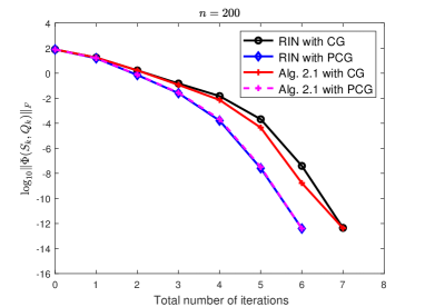
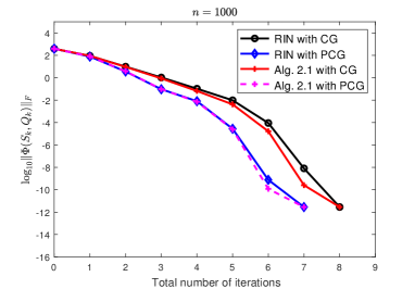
Figure 5.1: Convergence history of two tests for Example 5.4.

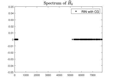
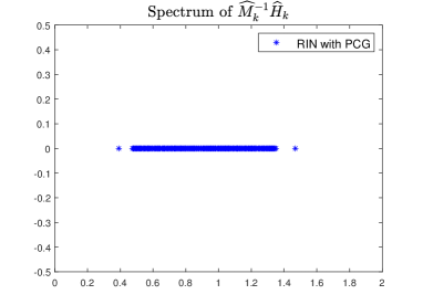
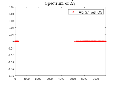
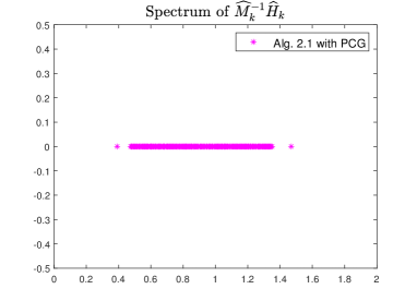
Figure 5.2: Spectrum of $\widehat{H}_{k}$ and $\widehat{M}_{k}^{-1}\widehat{H}_{k}$ at final iterates of one test for $n=100$.

6 Concluding remarks

In this paper, we consider the problem of reconstructing a symmetric nonnegative matrix from prescribed realizable spectrum. The inverse problem is reformulated as an underdetermined nonlinear matrix equation over a Riemannian product manifold. To solve the inverse problem, we develop a Riemannian underdetermined Newton dogleg method for finding a solution to a general underdetermined nonlinear equation defined between Riemannian manifold and Euclidean space. Under some mild assumptions, we show the proposed method converges globally and quadratically. Then we apply he proposed method to inverse problem by constructing an efficient preconditioner. Numerical results show the efficiency of the proposed method. In the future research, we will discuss how to construct an effective preconditioned numerical method for solving the inverse eigenvalue problem for nonsymmetric nonnegative matrices.

References

- [1] P.-A. Absil, R. Mahony, and R. Sepulchre, Optimization Algorithms on Matrix Manifolds, Princeton University Press, Princeton, 2008.
- [2] J. F. Bao, C. Li, W. P. Shen, J. C. Yao, and S. M. Guu, Approximate Gauss-Newton methods for solving underdetermined nonlinear least squares problems, Appl. Numer. Math., 111 (2017), pp. 92–110.
- [3] R. B. Bapat and T. E. S. Raghavan, Nonnegative Matrices and Applications, Cambridge University Press, Cambridge, UK, 1997.
- [4] A. Berman and R. J. Plemmons, Nonnegative Matrices in the Mathematical Sciences, Academic Press, New York, 1979.
- [5] X. Chen and D. L. Liu, Isospectral flow method for nonnegative inverse eigenvalue problem with prescribed structure, J. Comput. Appl. Math., 235 (2011), pp. 3990–4002.
- [6] X. J. Chen and T. Yamamotob, Newton-like methods for solving underdetermined nonlinear equations with nondifferentiable terms, J. Comput. Appl. Math., 59 (1994), pp. 311–324.
- [7] M. T. Chu, F. Diele, and I. Sgura, Gradient flow method for matrix completion with prescribed eigenvalues, Linear Algebra Appl., 379 (2004), pp. 85–112.
- [8] M. T. Chu and K. R. Driessel, Constructing symmetric nonnegative matrices with prescribed eigenvalues by differential equations, SIAM J. Math. Anal., 22 (1991), pp. 1372–1387.
- [9] M. T. Chu and G. H. Golub, Structured inverse eigenvalue problems, Acta Numer., 11 (2002), pp. 1–71.
- [10] M. T. Chu and G. H. Golub, Inverse Eigenvalue Problems: Theory, Algorithms, and Applications, Oxford University Press, Oxford, UK, 2005.
- [11] M. T. Chu and Q. Guo, A numerical method for the inverse stochastic spectrum problem, SIAM J. Matrix Anal. Appl., 19 (1998), pp. 1027–1039.
- [12] N. Echebest, M. L. Schuverdt, and R. P. Vignau, Two derivative-free methods for solving underdetermined nonlinear systems of equations, Comput. Appl. Math., 30 (2011), pp. 217-245.
- [13] N. Echebest, M. L. Schuverdt, and R. P. Vignau, A derivative-free method for solving box-constrained underdetermined nonlinear systems of equations, Appl. Math. Comput., 219 (2012), pp. 3198–3208.
- [14] R. Ellard and H. S̆migoc, Connecting sufficient conditions for the symmetric nonnegative inverse eigenvalues problem, Linear Algebra Appl., 498, (2016), pp. 521–552.
- [15] S. C. Eisenstat and H. F. Walker, Choosing the forcing terms in an inexact Newton method, SIAM J. Sci. Comput, 17 (1996), pp. 16–32.
- [16] P. D. Egleston, T. D. Lenker, and S. K. Narayan, The nonnegative inverse eigenvalue problem, Linear Algebra Appl., 379 (2004), pp. 475–490.
- [17] J. B. Francisco, N. Krejić, and J. M. Martínez, An interior point method for solving box-constrained underdetermined nonlinear systems, J. Comput. Appl. Math., 177 (2005) pp. 67–88.
- [18] G. H. Golub and C. F. Van Loan, Matrix Computations, 4th ed., Johns Hopkins University Press, Baltimore, 2013.
- [19] H. V. Henderson and S. R. Searle, Vet and vech operators for matrices, with some uses in Jacobians and multivariate statistics, Canad. J. Statist., 7 (1979), pp. 65–81.
- [20] C. R. Johnson, C. Marijuán, P. Paparella, and M. Pisonero, The NIEP, in: C. André, A. Bastos, A. Y. Karlovich, B. Silbermann, I. Zaballa (eds), Operator Theory, Operator Algebras, and Matrix Theory. Operator Theory: Advances and Applications, vol. 267, pp. 199-220, Birkhäuser, Cham, 2018.
- [21] C. R. Johnson and P. Paparella, Perron spectratopes and the real nonnegative inverse eigenvalue problem, Linear Algebra Appl., 493 (2016), pp. 281–300.
- [22] F. I. Karpelevic̆, On the characteristic roots of matrices with nonnegative elements, Izv. Akad. Nauk SSSR Ser. Mat. 15 (1951), pp. 361–383 (in Russian).
- [23] T. J. Laffey and H. Šmigoc, Nonnegative realization of spectra having negative real parts, Linear Algebra Appl., 416 (2006), pp. 148–159.
- [24] M. M. Lin, Fast recursive algorithm for constructing nonnegative matrices with prescribed real eigenvalues, Appl. Math. Comput., 256 (2015), pp. 582–590.
- [25] R. Loewy and D. London, A note on an inverse problems for nonnegative matrices, Linear Multilinear Algebra, 6 (1978), pp. 83–90.
- [26] D. G. Luenberger, Optimization by Vector Space Methods, John Wiley & Sons, New York, 1969.
- [27] J. M. Martinez, Quasi-Newton methods for solving underdetermined nonlinear simultaneous equations, J. Comput. Appl. Math., 34 (1991), pp. 171–190.
- [28] H. Minc, Nonnegative Matrices, John Wiley & Sons, New York, 1988.
- [29] G. N. de Oliveira, Nonnegative matrices with prescribed spectrum, Linear Algebra Appl., 54 (1983), pp. 117–121.
- [30] R. Orsi, Numerical methods for solving inverse eigenvalue problems for nonnegative matrices, SIAM J. Matrix Anal. Appl., 28 (2006), pp. 190–212.
- [31] P. Paparella, Realizing Suleimanova-type spectra via permutative matrices, Electron. J. Linear Algebra., 31, (2016), pp. 306–312.
- [32] R. P. Pawlowski, J. P. Simonis, H. F. Walker, and J. N. Shadid, Inexact Newton dogleg methods, SIAM J. Numer. Anal., 46 (2008), pp. 2112–2132.
- [33] R. Reams, An inequality for nonnegative matrices and the inverse eigenvalue problem, Linear Multilinear Algebra, 41 (1996), pp. 367–375.
- [34] E. Senata, Non-negative Matrices and Markov Chains, 2nd rev. ed., Springer-Verlag, New York, 2006.
- [35] R.L. Soto, Realizability criterion for the symmetric nonnegative inverse eigenvalue problem, Linear Algebra Appl., 416 (2006), pp. 783–794.
- [36] R.L. Soto, A family of realizability criteria for the real and symmetric nonnegative inverse eigenvalue problem, Numer. Linear Algebra Appl., 20 (2013), pp. 336–348.
- [37] G. W. Soules, Constructing symmetric nonnegative matrices, Linear and Multilinear Alg., 13 (1983), pp. 241–251.
- [38] J. P. Simons, Inexact Newton methods applied to underdetermined systems, PhD thesis. Department of Mathematical Science, Worcester Polytechnic Institute, 2006.
- [39] H. F. Walker and L. T. Watson, Least-change secant update methods for underdetermined systems, SIAM J. Numer. Anal., 27 (1990), pp. 1227–1262.
- [40] S. F. Xu, An Introduction to Inverse Algebraic Eigenvalue Problems, Beijing; Friedr. Vieweg & Sohn, Braunschweig, 1998.
- [41] Z. Zhao, Z. J. Bai, and X. Q. Jin, A Riemannian inexact Newton-CG method for constructing a nonnegative matrix with prescribed realizable spectrum, Numer. Math., 140 (2018), pp. 827–855.