Large deviations principle for the cubic NLS equation

Abstract.

In this paper, we present a probabilistic study of rare phenomena of the cubic nonlinear Schrödinger equation on the torus in a weakly nonlinear setting. This equation has been used as a model to numerically study the formation of rogue waves in deep sea. Our results are twofold: first, we introduce a notion of criticality and prove a Large Deviations Principle (LDP) for the subcritical and critical cases. Second, we study the most likely initial conditions that lead to the formation of a rogue wave, from a theoretical and numerical point of view. Finally, we propose several open questions for future research.

1. Introduction

1.1. Motivation and background

In the last few decades there has been considerable research in the field of dispersive equations, and particularly on the nonlinear Schrödinger (NLS) equation:

(1.1) $$\begin{cases}i{\partial}_{t}u+\Delta u=\mu\,|u|^{2}\,u,\qquad\mu=\pm 1,\\ u|_{t=0}=u_{0}\,.\end{cases}$$

One of the most fundamental questions is that of existence and uniqueness of solutions. The question of well-posedness on $\mathbb{R}^{d}$ was extensively studied in the 1980s and the 1990s for subcritical initial data [14, 37, 45, 62] and later for energy and mass critical initial data [9, 39, 15, 63, 31]. Well-posedness on the torus $\mathbb{T}^{d}$ received much attention in the 1990s, mainly due to Bourgain’s breakthrough paper [6], which was followed by work in [41, 44, 65]. These results are deterministic, in the sense that one shows that a solution exists for every initial datum $u_{0}$ in a certain space, typically Sobolev spaces such as $H^{s}$ where the regularity $s$ must be larger or equal to a critical value $s_{c}$.

Beyond existence of solutions, it is important to understand the long-time behaviour of such solutions. In $\mathbb{R}^{d}$ solutions to (1.1) with $\mu=1$ and in the critical and subcritical case scatter (sometimes under some technical conditions), see for example [37, 15, 63, 31, 61, 64], while in the super critical case blow-up may occur, see the recent work [36]. In the case $\mu=-1$, some solutions to (1.1) blow up in finite time, and therefore they cannot be extended indefinitely, see for example [52, 36]. In contrast to this generic behavior, certain types of initial data give rise to traveling waves and soliton solutions, see [1] and the references therein. These solutions display an unusual long-term behavior, and as a result they are considered rare phenomena.

On the torus $\mathbb{T}^{d}$, scattering is not possible so one expects different asymptotics. In particular, it is of great physical interest to analyse phenomena related to weak turbulence, and more precisely that of energy transfer. With this we mean the expected behaviour of certain initial data with frequency localised support that evolve into solutions whose support lives mostly in higher frequencies. This phenomenon is connected to the question of asymptotic growth of Sobolev norms of solutions to the Schrödinger equation whose study was started by Bourgain [10] and later continued in [58, 57, 60, 26, 25, 43, 55, 4, 13, 16, 40] among others. In addition to such theoretical results, there are many interesting simulations and experimental results about transfer of energy to high frequencies, see for example [51, 17, 42, 43].

In 1988, the work of Lebowitz, Rose, and Speer [46], followed by Bourgain’s papers on invariant measures [7, 8], started the probabilistic study of solutions to the nonlinear Schrödinger equation in a context in which until then harmonic and Fourier analysis had been the predominant and preferred tools of investigation. In such works, one typically considers random initial data, whose Fourier coefficients are normally distributed. This viewpoint has been extensively used to obtain generic results which hold for almost every initial datum (i.e. almost surely). For example, this additional flexibility led in many cases to an improved well-posedness theory, see for example [32, 29, 30]. The random data theory has also been fundamental in the study of the long-term behaviour of solutions to (1.1) on $\mathbb{T}^{d}$ that we mentioned above. Indeed, one of the most interesting lines of research in this direction is the derivation of the Wave Kinetic Equation (WKE), which connects the study of the typical size of the Fourier coefficients of the solution to (1.1) to the study of solutions to a kinetic equation [11, 18, 19, 28, 27, 59]. All such works make the most of probabilistic estimates to argue that non-generic behavior is unlikely, but few of them focus on the study of such non-generic behavior.

In this paper, we study rogue waves as an interesting and still not well understood example of rare phenomena. Oceanographers generally define rogue waves to be deep-water waves whose amplitude exceeds twice the characteristic wave height expected for the given surface conditions [22, 34]. Over the past decades, there has been considerable interest in modelling rogue waves, both because analytically their origins are still mysterious and because their sudden appearances pose a threat for a variety of naval infrastructure.

Several evolution equations have been classically used as models for the study of rogue waves. Two of the most popular models are given by the cubic Schrödinger equation and the Dysthe equation. The Dysthe equation has been the subject of many experimental and computational works, for instance [22, 33, 35]; as well as some theoretical results, e.g. [38, 53]. A few variants of the NLS equation have also been used to model rogue wave formation, see [21, 54] among others. Note that all these models are derived from the incompressible Navier-Stokes equation, after truncating an asymptotic expansion of the modulation of a wavetrain at various orders [33, 53].

There are several theories to explain the precise mechanism for the formation of rogue waves [54], but this phenomenon is still the subject of much debate. In the case of the focusing NLS equation in $\mathbb{R}$, Bertola and Tovbis obtained a precise description of a deterministic class of solutions near their peak [5]. One of the goals of this paper is to provide a characterization of rogue waves of the weakly nonlinear NLS equation on $\mathbb{T}=[0,2\pi]$ with random initial data.

The results in this paper are inspired by some recent work of Dematteis, Grafke, Onorato, and Vanden-Eijnden [21, 22, 23]. In these papers, the authors conjecture the existence of a Large Deviation Principle that may be used to predict and study the formation of rogue waves. More precisely, they consider an equation akin to (1.1) with $\mu=-1$ on a circle of fixed size $L$, with random initial data $u_{0}$ of the form

(1.2) $$u_{0}(x)=\sum_{|k|\leq N}\vartheta_{k}e^{ik\cdot x}.$$

Here, the set of initial data is parametrized by $\vartheta=(\vartheta_{k})_{|k|\leq N}\in\mathbb{C}^{2N+1}$. In order to make $u_{0}$ random, the authors endow the space of parameters $\mathbb{C}^{2N+1}$ with a probability measure such that $\left\{\vartheta_{k}\right\}_{|k|\leq N}$ are independent and identically distributed (i.i.d.) complex Gaussian random variables with $\mathbb{E}\vartheta_{k}=\mathbb{E}\vartheta_{k}^{2}=0$ and $\mathbb{E}|\vartheta_{k}|^{2}=c_{k}^{2}$, for some fast-decaying $c_{k}>0$.

For $t>0$ and $z>0$ fixed, the set of initial data that generate a rogue wave of height at least $z$ at time $t$ is given by

(1.3) $$\mathcal{D}(t,z):=\left\{(\vartheta_{k})_{|k|\leq N}\in\mathbb{C}^{2N+1}\Big{|}\sup_{x\in[0,L]}|u(t,x\,|\,\vartheta)|>z\ \right\}$$

where $u$ is the solution to the equation with initial data (1.2).

In order to quantify the likelihood of $\mathcal{D}(t,z)$, Dematteis et al. propose a theoretical framework that allows them to conclude a large deviations principle (LDP), provided that the minimization problem

(1.4) $$\vartheta^{\ast}(z)=\underset{\vartheta\in\mathcal{D}(t,z)}{\mathrm{argmin}}\,\,\mathcal{I}(\vartheta).$$

has a unique solution, where

$$\mathcal{I}(\vartheta)=\max_{y\in\mathbb{C}^{2N+1}}[\,\langle y,\vartheta\rangle-S(y)]\qquad\mbox{and}\quad S(y)=\log\mathbb{E}e^{\langle y,\vartheta\rangle}.$$

In particular, for a fixed $t>0$ and as $z\rightarrow\infty$, they claim that

(1.5) $$\log{\mathbb{P}}(\mathcal{D}(t,z))=-\mathcal{I}(\vartheta^{\ast}(z))+o(1).$$

The goal of this paper is to prove rigorously conjecture (1.5) in the case of the NLS equation with a weak nonlinearity. The application of the theoretical framework proposed by Dematteis et al. requires verifying a set of strong assumptions that are very difficult to check in practice, such as bounds on the gradient $\nabla_{\vartheta}\sup_{x\in[0,L]}|u(t,x\,|\,\vartheta)|$ or the convexity of the set $\mathcal{D}(t,z)$, so that the existence of a unique minimizer for (1.4) is guaranteed.

For these reasons, we follow a different approach that allows us to establish an LDP of the form

(1.6) $$\log{\mathbb{P}}\left(\sup_{x\in\mathbb{T}}|u(t,x)|>z\right)=-I(z)+o(1),\quad\mbox{as}\ z\rightarrow\infty,$$

where we can derive the rate function $I$ without having to solve the minimization problem in (1.4). In (1.6), $u$ is the solution to the equation with initial data of the form (1.2) with an infinite number of Fourier modes ($N=\infty$). See 1.1 below for a precise statement.

In the second part of the paper, we investigate the following question: “Conditioned on the fact that we observe a rogue wave of height at least $z>0$ at time $t>0$, what is the most likely initial datum that generates such phenomenon?” To answer this question, we recover the minimization problem given by the right-hand side of (1.4), and show that it admits a two-parameter family of solutions. In addition, we can construct neighborhoods $\mathcal{U}(t,z)$ around the family of minimizers whose probability is almost identical to that of $\mathcal{D}(t,z)$. See 1.9 below for a precise statement.

1.2. Statement of results

In this paper, we focus on the cubic Schrödinger equation on the torus $\mathbb{T}=[0,2\pi]$ with a weak nonlinearity:

(1.7) $$\begin{cases}i{\partial}_{t}u+\Delta u=\mu\,\varepsilon^{\alpha}|u|^{2}\,u\\ u(t,x)|_{t=0}=u_{0}\end{cases}$$

for $\alpha\geq 0$ and $\mu=\pm 1$, and where the parameter $\varepsilon>0$ controls the size of the nonlinearity. We consider random initial data of the form:

(1.8) $$u_{0}(x)=\sum_{k\in\mathbb{Z}}c_{k}\eta_{k}e^{ikx}$$

where

1. the coefficients have the form $c_{k}=a\,e^{-b|k|}$, or $c_{k}=a\,e^{-b|k|^{2}}$, for all $k\in\mathbb{Z}$, where $a,b>0$ are fixed; and

2. $\{\eta_{k}\}_{k\in\mathbb{Z}}$ are independent, identically distributed, complex Gaussian random variables with $\mathbb{E}\eta_{k}=0$, $\mathbb{E}\eta_{k}\eta_{j}=0$ and $\mathbb{E}\eta_{k}\overline{\eta}_{j}=\delta_{kj}$ for $k,j\in\mathbb{Z}$.

Assumption (1) is based on the choice of coefficients in [22], but our results extend to other families of coefficients, see 1.3. In the sequel we assume that $a=1$ since we can rescale the equation if that is not the case.

Our first result is a rigorous proof of (1.6) for solutions to (1.7) with $\alpha=2$ and initial data of the form (1.8).

Theorem 1.1 (Large Deviation Principle).

Consider the NLS equation on the circle $\mathbb{T}=[0,2\pi]$:

(1.9) $$\begin{cases}i{\partial}_{t}u+\Delta u=\varepsilon^{2}|u|^{2}\,u\\ u(0,x)=\sum_{k\in\mathbb{Z}}c_{k}\eta_{k}e^{ikx}\end{cases}$$

with initial data as in (1.8). Consider the probability of seeing a large wave of height $z(\varepsilon):=z_{0}\,\varepsilon^{-1/2}>0$ at time $t>0$ and fixed $z_{0}>0$. If $t\lesssim\varepsilon^{-1}$ we have that

(1.10) $$\lim_{\varepsilon\rightarrow 0^{+}}\varepsilon\,\log{\mathbb{P}}\left(\sup_{x\in\mathbb{T}}|u(t,x)|>z_{0}\,\varepsilon^{-1/2}\right)=-\frac{z_{0}^{2}}{\sum_{k\in\mathbb{Z}}c_{k}^{2}}.$$

Remark 1.2.

The requirement that $t\lesssim\varepsilon^{-1}$ is connected to the criticality of the problem. This notion of criticality is discussed in 1.7. The proof of 1.1 is based on approximating the solution $u$ by a function that satisfies (1.10). For subcritical times $t\ll\varepsilon^{-1}$, a linear approximation suffices. For critical times $t=\mathcal{O}(\varepsilon^{-1})$, the linear approximation is not enough, and we must use a resonant approximation instead.

Remark 1.3.

The coefficients $c_{k}$ given in (1.8) are based on those in [22], which are chosen to model observations in the North Sea. Finding the optimal family of coefficients (in terms of decay) so that (1.10) holds is an interesting open question.

Remark 1.4.

We have stated 1.1 for the defocusing equation, but our results extend to the focusing equation. In fact the sign of the nonlinearity has no effect in our results since we are in a weakly nonlinear regime. As we will show below, our results are strongly based on the special form that a linear solution takes in the 1D setting, as well as the resonant set in this dimension. We speculate though that a possible extension to a 2D setting may be possible for irrational tori. There in fact, it has been proved [43] that the irrationality of the torus completely decouples the resonant set into two 1D resonant sets, one for each coordinate.

Remark 1.5.

The cubic NLS equation on $\mathbb{T}$ is an integrable system, however our results are related to neither integrability nor blow-up. We note that our initial data live in $\cap_{s>0}H^{s}(\mathbb{T})$ almost surely, thus a unique global solution exists almost surely. The question of rogue waves is related to the $L^{\infty}(\mathbb{T})$-norm of the solutions and their growth over time. Most solutions to the equation will barely grow over time. As shown in Section 5, rogue waves will typically peak at a certain point in space and time and decrease in size quickly after.

The factor of $\varepsilon^{2}$ in front of the cubic nonlinearity in 1.1 is motivated by the standard notation in the PDE literature. However, our techniques can handle the more general scenarios presented below. For the sake of concreteness, we will limit ourselves to the setting in 1.1 in the rest of the paper.

Theorem 1.6.

Consider the NLS equation on the torus $\mathbb{T}=[0,2\pi]$:

$$\begin{cases}i{\partial}_{t}u+\Delta u=\varepsilon^{\alpha}\,|u|^{2}\,u\\ u(0,x)=\sum_{k\in\mathbb{Z}}c_{k}\eta_{k}e^{ikx},\end{cases}$$

where $\alpha>0$, and initial data as in (1.8). Consider the probability of seeing a large wave of height $z(\varepsilon):=z_{0}\varepsilon^{-1/2}$ at time $t\sim\varepsilon^{-\beta}$ for some $\beta\in\mathbb{R}$. Then we have that:

• If $\alpha-1>\beta$, then (1.10) holds.

• If $\alpha-1=\beta$ and $\beta>0$, then (1.10) holds.

Remark 1.7.

Let us motivate the range of parameters in 1.6. First we rewrite (1.7) by using Duhamel formula:

$$u(t)=e^{it\Delta}u_{0}+u_{\mathrm{nl}}(t)=e^{it\Delta}u_{0}+\varepsilon^{\alpha}\,\int_{0}^{t}e^{i(t-t^{\prime})\Delta}|u|^{2}u(t^{\prime})\,dt^{\prime}.$$

At a certain fixed time $t$ (independent of $\varepsilon$) we impose the condition of seeing a rogue wave of size $\varepsilon^{-1/2}$, i.e. $\left\lVert u(t)\right\rVert_{L^{\infty}(\mathbb{T})}>\varepsilon^{-1/2}$. Next we estimate the nonlinear term $u_{\mathrm{nl}}(t)$ in some space $X$ which embeds continuously into $L^{\infty}(\mathbb{T})$. In this paper, we use various Fourier-Lebesgue spaces such as $X={\mathcal{F}}L^{0,1}$, but other choices such as $X^{s,b}$ spaces introduced by Bourgain in [6] are possible. Then we have that

$$\varepsilon^{-1/2}<\left\lVert u(t)\right\rVert_{L^{\infty}_{x}}\leq\left\lVert u(t)\right\rVert_{X},$$

and

$$\left\lVert u_{\mathrm{nl}}(t)\right\rVert_{X}=\varepsilon^{\alpha}\,\left\lVert\int_{0}^{t}e^{i(t-t^{\prime})\Delta}|u|^{2}u(t^{\prime})\,dt^{\prime}\right\rVert_{X}\lesssim\varepsilon^{\alpha}\,\left\lVert u\right\rVert_{X}^{3}.$$

Note that the right-hand side is at least as large as $\varepsilon^{\alpha-3/2}$ (but it might be much larger!). Assuming that this trilinear estimate is sharp, we say that the problem is subcritical if $\alpha-3/2<-1/2$, critical if $\alpha-3/2=-1/2$ and supercritical otherwise. This explains the range of parameters in 1.6 when $\beta=0$. The notion of criticality may be extended to times $t$ which depend on $\varepsilon$ by rescaling the equation.

Remark 1.8.

Note that 1.1 corresponds to the choice $\alpha=2$. An interesting open question would be to understand the critical case $(\alpha,\beta)=(1,0)$, as well as any supercritical cases such as $\alpha=0$ (fully non-linear regime). In fact, in the case $\alpha=0$, the numerical experiments in [21, 22, 23] suggest that the probability of seeing a rogue wave decays at a slower speed. This would correspond to a non-Gaussian scaling in (1.10) with a sub-quadratic rate function $I(\cdot)$ in (1.6).

Our work constitutes a first step towards solving this more challenging problem, and proposes a framework to tackle the non-linear problem via approximating the solution of (1.9) and deriving explicit probability bounds for this approximation.

1.1 allows us to quantify the probability that we observe a rogue wave. Despite being rare, rogue waves can actually happen. Our next result investigates the following question: “Conditioned on the fact that we observe a rogue wave of height at least $z>0$ at time $t>0$, what is the most likely initial datum that generates such phenomenon?” To answer this question, we introduce the set

$$\mathcal{H}=\{(r_{k},\phi_{k})_{k\in\mathbb{Z}}\mid r_{k}\geq 0,\ \phi_{k}\in[0,2\pi)\},$$

and endow it with a probability measure such that $r_{k}e^{i\phi_{k}}$ are distributed as independent complex Gaussian as in (1.8). Then, we can parametrize the space of initial data as follows:

$$\vartheta=(r_{k},\phi_{k})_{k\in\mathbb{Z}}\in\mathcal{H}\mapsto u_{0}(x\mid\vartheta)=\sum_{k\in\mathbb{Z}}c_{k}r_{k}e^{ikx+i\phi_{k}}.$$

As we explain in Section 5, the question of finding the most likely initial data is connected to a certain minimization problem over the set

(1.11) $$\mathcal{D}(t,z_{0}\varepsilon^{-1/2})=\left\{\vartheta\in\mathcal{H}\ \Big{|}\ \sup_{x\in\mathbb{T}}|u(t,x\mid\vartheta)|>z_{0}\varepsilon^{-1/2}\right\}.$$

The solution to this minimization problem when $u$ is the solution of the linear Schrödinger equation yields a two-parameter family of initial data given by:

(1.12) $$\begin{split}r_{k}^{*}&:=\frac{c_{k}z_{0}\varepsilon^{-1/2}}{\sum_{j\in\mathbb{Z}}c_{j}^{2}},\\ \phi^{*}_{k}&:=\phi^{*}_{0}-kx^{*}+k^{2}t\,\left(\text{mod }2\pi\right),\end{split}$$

where $x^{\ast}\in\mathbb{T}$ parametrizes the position of the peak of the rogue wave, and $\phi^{\ast}_{0}\in[0,2\pi)$ parametrizes the phase of the Fourier mode associated with $c_{0}$.

The main result in Section 5 shows that this special family of initial data concentrates as much probability as the entire set of rogue waves (1.11). In order to state this theorem, we construct a small neighborhood $\mathcal{U}(\varepsilon)$ around this family, given by the $\vartheta=(r_{k},\phi_{k})_{k\in\mathbb{Z}}$ satisfying:

(1.13) $$\begin{split}r_{k}^{\ast}\leq r_{k}&\leq r_{k}^{\ast}+\varepsilon^{2/5}\qquad\mbox{for all}\ |k|\leq-\frac{1}{b}\log\left(\frac{2\sum_{j\in\mathbb{Z}}c_{j}^{2}}{z_{0}}\,\varepsilon^{9/10}\right),\\ |\phi_{k}-\phi_{k}^{\ast}|&\leq\varepsilon\qquad\mbox{for all}\ |k|\leq\varepsilon^{-1/2}\ \mbox{except $k=0,1$}.\end{split}$$

Theorem 1.9.

Consider the set $\mathcal{U}(\varepsilon)$ given by (1.12)-(1.13). Then $\mathcal{U}(\varepsilon)$ satisfies the same LDP, (1.10), as the set of rogue waves (1.11). Moreover, $\mathcal{U}(\varepsilon)$ is almost entirely contained in the set $\mathcal{D}(t,z_{0}\varepsilon^{-1/2}-\varepsilon)$. More precisely,

(1.14) $$\log{\mathbb{P}}\left(\mathcal{U}(\varepsilon)-\mathcal{D}(t,z_{0}\varepsilon^{-1/2}-\varepsilon)\right)\lesssim-\exp(c\varepsilon^{-1/2}))\qquad\mbox{as}\ \varepsilon\rightarrow 0^{+}.$$

Remark 1.10.

The construction of the set $\mathcal{U}(\varepsilon)$ in 1.9 is based on the linear Schrödinger equation. However, one can adapt this construction to tackle the nonlinear equation up to times given by 1.1. See Section 5 for more details.

Finally, we list a series of interesting open questions at the end of Section 5. Furthermore, we complement this theoretical analysis with some simulations to illustrate how the family of initial data given by (1.12) behaves as time passes.

1.3. Ideas of the proof

1.3.1. Main ideas in 1.1

At a conceptual level, the proof of 1.6 and that of 1.1 are similar, so let us focus on the latter. The main ideas of the proof of 1.1 are: (a) finding a good approximation $u_{\mathrm{app}}$ to the solution to the NLS equation (1.9), and (b) proving a LDP akin to (1.10) for $u_{\mathrm{app}}$. For small times $t\ll\varepsilon^{-1}$, the linear flow constitutes a good approximation, whereas larger times require the use of a resonant approximation.

The resonant approximation is an explicit solution to an equation similar to (1.9), where we replace the nonlinearity $\varepsilon^{2}|u|^{2}u$ by a different cubic nonlinearity that captures the main contribution of $\varepsilon^{2}|u|^{2}u$ to the equation over timescales $t=\mathcal{O}(\varepsilon^{-1})$. This approximation has the form:

(1.15) $$u_{\mathrm{app}}(t,x)=e^{2it\varepsilon^{2}\,M}\,\sum_{k\in\mathbb{Z}}c_{k}\eta_{k}\,e^{ikx+i\varepsilon^{2}t\,c_{k}^{2}|\eta_{k}|^{2}-it|k|^{2}}$$

where $M=\left\lVert u(t)\right\rVert_{L^{2}(\mathbb{T})}^{2}$ is the mass, which is conserved. Further details are provided in Section 4.1. Such approximations have been used by Carles, Dumas and Sparber [12] and Carles and Faou [13] in the context of instability of the periodic NLS equation and energy cascades, respectively.

Intuitively, the reason why $\sup_{x\in\mathbb{T}}|u_{\mathrm{app}}(t,x)|$ remains sub-Gaussian is that nonlinear effects are restricted to the phases of the Fourier coefficients, while the moduli are unchanged. It is unclear whether this holds in other regimes beyond those given by 1.6, especially so in the case of the focusing NLS equation.

Both the linear and resonant approximations satisfy an LDP of the form (1.10). The first ingredient in the proof of 1.1 is a general result in Large Deviations Theory known as the Gärtner-Ellis theorem, see Section 2 as well as 4.1. This classic result in Probability Theory uses convex analysis to state that an LDP for a family of probability measures, $\left\{\mu_{\varepsilon}\right\}_{\varepsilon>0}$, holds provided that the limit of their re-scaled cumulant-generating functions exists and enjoys some good regularity properties.

The second ingredient in the proof of 1.1 is a bootstrapping argument, which shows that a large difference between the actual solution to (1.9) and our approximation must be a result of an even larger initial datum $u_{0}$. Such large initial data are very unlikely, which allows us to replace the actual solution $u(t,x)$ in (1.10) by the approximation $u_{\mathrm{app}}(t,x)$ up to a negligible error. As a result one can extend the LDP from $u_{\mathrm{app}}$ to $u$.

1.3.2. Main ideas in 1.9

The goal of this result is to show that the most likely way in which rogue wave arise in this weakly nonlinear context is due to phase synchronization. The construction of the one-sided neighborhood $\mathcal{U}(\varepsilon)$ in (1.13) is based on two-scales: we control the moduli of $\mathcal{O}(|\log\varepsilon|)$ Fourier modes, but we force $\mathcal{O}(\varepsilon^{-1/2})$ phases to almost synchronize at a certain point in space and time.

In 5.3, we exploit the fact that our construction is explicit to show that $\mathcal{U}(\varepsilon)$ satisfies the same LDP as that in 1.1 by an elementary argument. The key result, however, is to show that the elements in $\mathcal{U}(\varepsilon)$ are almost exclusively rogue waves. To prove this we must quantify the probability that the Fourier modes that we do not control in $\mathcal{U}(\varepsilon)$ work against us and create cancellation. Loosely speaking, this is achieved by proving the estimate

$$\sup_{x\in\mathbb{T}}|u(t,x)|^{2}\geq\left(\sum_{|k|\lesssim|\log\varepsilon|}c_{k}|\eta_{k}|\right)^{2}+E(\varepsilon)$$

for some explicit error function $E(\varepsilon)$. The key argument in the proof of 1.9 is a careful analysis of this error function, which shows that it is very close to zero with very high probability.

1.4. Outline

In Section 2, we develop a LDP for the linear Schrödinger equation (1.7) (with $\mu=0$). In Section 3, we prove 1.1 for subcritical times. In Section 4, we introduce the resonant approximation and prove 1.1 for critical times. Finally, in Section 5 we motivate and study the minimization problem that leads to (1.12). Moreover, we prove 1.9 and conduct numerical simulations about the “most typical” rogue waves.

1.5. Notation

We write $A\lesssim B$ to indicate an estimate of the form $A\lesssim CB$ for some positive constant $C$ which may change from line to line. The inequality $A\lesssim_{d}B$ indicates that the implicit constant $C$ depends on $d$.

We also employ the big $\mathcal{O}$ notation $A=\mathcal{O}_{d}(B)$, which means that $A\lesssim B$ as $d\rightarrow 0$. For a real number $a$, the notation $a-$ means $a-\varepsilon$ for $0<\varepsilon\ll 1$ small enough. Similarly, $a+$ means $a+\varepsilon$ for $0<\varepsilon\ll 1$ small enough.

For $1\leq p\leq\infty$ we often work in the space $L^{p}([a,b])$, which consists of functions $f:[a,b]\rightarrow\mathbb{C}$ such that

$$\left\lVert f\right\rVert_{L^{p}}=\left(\int_{a}^{b}|f(x)|^{p}\,dx\right)^{1/p}<\infty,$$

with the usual modifications when $p=\infty$. Similarly, $\ell^{p}$ consists of sequences $f=(f_{k})_{k\in\mathbb{Z}}$, $f_{k}\in\mathbb{C}$, such that

$$\left\lVert f\right\rVert_{\ell^{p}}=\left(\sum_{k\in\mathbb{Z}}|f_{k}|^{p}\right)^{1/p}<\infty.$$

In Section 3 and Section 4 we work in Fourier-Lebesgue spaces ${\mathcal{F}}L^{s,p}={\mathcal{F}}L^{s,p}(\mathbb{T})$ with $s\in\mathbb{R}$ and $1\leq p\leq\infty$. These are spaces of functions $f:\mathbb{T}\rightarrow\mathbb{C}$ whose Fourier coefficients $(f_{k})_{k\in\mathbb{Z}}$ have the following finite norm:

$$\left\lVert f\right\rVert_{{\mathcal{F}}L^{s,p}}=\left\lVert\langle k\rangle^{s}f_{k}\right\rVert_{\ell_{k}^{p}}=\left(\sum_{k\in\mathbb{Z}}\langle k\rangle^{ps}\,|f_{k}|^{p}\right)^{1/p}=\left(\sum_{k\in\mathbb{Z}}(1+|k|)^{ps}\,|f_{k}|^{p}\right)^{1/p}.$$

Finally, we denote $H^{s}(\mathbb{T})=\mathcal{F}L^{s,2}(\mathbb{T})$ as usual.

1.6. Acknowledgements

We thank Eric Vanden-Eijnden and Miguel Onorato for their suggestions and helpful discussions about their work. The first author also thanks Promit Ghosal for some rich conversations about Large Deviations Theory.

2. Large Deviations Principle for the linear Schrödinger equation

Consider the linear Schrödinger equation on the torus $\mathbb{T}=[0,2\pi]$:

(2.1) $$\left\{\begin{array}[]{l}i\,{\partial}_{t}u+\Delta u=0,\\ u(t,x)|_{t=0}=u_{0},\end{array}\right.$$

where the random initial data, $u_{0}$, is given as in (1.8). Our goal is to estimate

$${\mathbb{P}}\left(\sup_{x\in\mathbb{T}}|u(t,x)|\geq z(\varepsilon)\right)$$

sharply, for some fixed $t\in\mathbb{R}$ and $z(\varepsilon)$ large. More concretely, we want to obtain a Large Deviations Principle (LDP) for $\sup_{x\in\mathbb{T}}|u(t,x)|$. This requires that we find a lower semi-continuous function, $I:[0,+\infty)\mapsto[0,+\infty]$, and a real number $\alpha>0$, such that, for any $z_{0}>0$ fixed, we have

(2.2) $$-\inf_{z\in(z_{0},+\infty)}I(z)\leq\liminf_{\varepsilon\rightarrow 0^{+}}\varepsilon^{\alpha}\log\left({\mathbb{P}}\left(\sup_{x\in\mathbb{T}}|u(t,x)|\geq z_{0}\varepsilon^{-1/2}\right)\right),$$

and

(2.3) $$\limsup_{\varepsilon\rightarrow 0^{+}}\varepsilon^{\alpha}\log\left({\mathbb{P}}\left(\sup_{x\in\mathbb{T}}|u(t,x)|\geq z_{0}\varepsilon^{-1/2}\right)\right)\leq-\inf_{z\in[z_{0},+\infty)}I(z).$$

We gather these results in the following proposition.

Proposition 2.1.

Consider the linear Schrödinger equation on the torus $\mathbb{T}=[0,2\pi]$ as in (2.1), with random initial data given by $u_{0}=\sum_{k\in\mathbb{Z}}c_{k}\eta_{k}e^{ikx}$, presented in (1.8). Then,

(2.4) $$\lim_{\varepsilon\rightarrow 0^{+}}\varepsilon\,\log{\mathbb{P}}\left(\left\lVert e^{-it\Delta}u_{0}\right\rVert_{L^{\infty}_{x}}>z_{0}\,\varepsilon^{-1/2}\right)=-\frac{z_{0}^{2}}{\sum_{k\in\mathbb{Z}}c_{k}^{2}},$$

for any $t\in\mathbb{R}$ and $z_{0}>0$. In particular, (2.2) and (2.3) are satisfied with rate function $I(z)=\frac{z^{2}}{\sum_{k\in\mathbb{Z}}c_{k}^{2}}$ and $\alpha=1$.

Remark 2.2.

A posteriori we see that our choice for $I$ is actually continuous, and hence

$$\inf_{z\in[z_{0},+\infty)}I(z)=\inf_{z\in(z_{0},+\infty)}I(z).$$

This implies that (2.2) and (2.3) is actually a chain of equalities, and we can prove the stronger result presented in (2.4).

Remark 2.3.

It is worth noticing that $I$ is a quadratic function. This corresponds to a sub-Gaussian behavior for the tails of $\sup_{x\in\mathbb{T}}|u(t,x)|$. Nevertheless, it is easy to see that $\sup_{x\in\mathbb{T}}|u(t,x)|$ itself is not Gaussian.

Remark 2.4.

In the Probability literature, Lindgren studied various path properties of Gaussian fields around its local maxima in a series of papers [47, 48, 49, 50]. However, these results do not apply directly to our work since we are interested in establishing an LDP for the global maxima on the space variable.

We divide the proof of 2.1 into two parts: first, we establish the lower bound, which follows from the fact that we can explicitly derive the distribution of $u(t,x)$, for a fixed pair $(t,x)\in\mathbb{R}\times\mathbb{T}$; and then, we prove the upper bound estimating from above $\sup_{x\in\mathbb{T}}|u(t,x)|$, and applying the Gärtner-Ellis Theorem.

2.1. Lower Bound

The solution $u$ for the linear flow in (2.1) can be written as

(2.5) $$u(t,x)=e^{-it\Delta}u_{0}(x)=\sum_{k\in\mathbb{Z}}c_{k}\eta_{k}\,e^{i\,kx-i\,k^{2}t},$$

for $(t,x)\in\mathbb{R}\times\mathbb{T}$. Since all the terms in the sum are independent complex normal random variables, so is $u(t,x)$ as long as $\sum_{k\in\mathbb{Z}}{\mathbb{E}}\left[u^{k}(t,x)\right]$, $\sum_{k\in\mathbb{Z}}{\mathbb{E}}\left[u^{k}(t,x)u^{k}(t,x)\right]$, and $\sum_{k\in\mathbb{Z}}{\mathbb{E}}\left[u^{k}(t,x)\overline{u^{k}(t,x)}\right]$ converge, where $u^{k}(t,x):=c_{k}\eta_{k}\,e^{i\,kx-i\,k^{2}t}$. It is easy to see that

$$\sum_{k\in\mathbb{Z}}{\mathbb{E}}\left[u^{k}(t,x)\right]=\sum_{k\in\mathbb{Z}}c_{k}{\mathbb{E}}\left[\eta_{k}\right]e^{i\,kx-i\,k^{2}t}=0,$$

$$\sum_{k\in\mathbb{Z}}{\mathbb{E}}\left[u^{k}(t,x)u^{k}(t,x)\right]=\sum_{k\in\mathbb{Z}}c_{k}^{2}{\mathbb{E}}\left[\eta_{k}\eta_{k}\right]e^{i\,2kx-i\,2k^{2}t}=0,$$

and

$$\sum_{k\in\mathbb{Z}}{\mathbb{E}}\left[u^{k}(t,x)\overline{u^{k}(t,x)}\right]=\sum_{k\in\mathbb{Z}}c_{k}^{2}{\mathbb{E}}\left[\eta_{k}\bar{\eta_{k}}\right]=\sum_{k\in\mathbb{Z}}c_{k}^{2}<\infty.$$

Therefore, for $(t,x)\in\mathbb{R}\times\mathbb{T}$ fixed, $u(t,x)$ is a complex Gaussian distribution with mean $0$ and variance $\sum_{k\in\mathbb{Z}}c_{k}^{2}$. It is worth noting that this distribution depends neither on $t$ nor on $x$. That is, as a random field, $(t,x)\mapsto u(t,x)$ is at stationarity.

It is a well-known result in Probability [56] that the modulus of a complex Gaussian random variable with mean $0$ and variance $2\sigma^{2}$ follows a Rayleigh distribution with parameter $\sigma>0$ and probability density function

(2.6) $$f(x\,|\,\sigma)=\frac{x}{\sigma^{2}}e^{-\frac{x^{2}}{2\sigma^{2}}},\qquad x\geq 0.$$

This fact allows us to compute the lower bound as follows:

$${\mathbb{P}}\left(\sup_{x\in\mathbb{T}}|u(t,x)|\geq z_{0}\varepsilon^{-1/2}\right)\geq{\mathbb{P}}\left(|u(t,0)|\geq z_{0}\varepsilon^{-1/2}\right)$$

$$=\int_{z_{0}\varepsilon^{-1/2}}^{+\infty}\frac{2x}{\sum_{k\in\mathbb{Z}}c_{k}^{2}}\exp\left(-\frac{x^{2}}{\sum_{k\in\mathbb{Z}}c_{k}^{2}}\right)dx=\exp\left(-\frac{z_{0}^{2}\varepsilon^{-1}}{\sum_{k\in\mathbb{Z}}c_{k}^{2}}\right).$$

Hence, if we take $\alpha=1$ and define $I(z):=\frac{z^{2}}{\sum_{k\in\mathbb{Z}}c_{k}^{2}}$, we can establish (2.2), as we wanted.

2.2. Upper bound

Since $\eta_{k}$ is a standard complex Gaussian, we can write $\eta_{k}$ as $R_{k}e^{i\varphi_{k}}$, where $R_{k}\stackrel{{\scriptstyle i.i.d.}}{{\sim}}Rayleigh(1/\sqrt{2})$ and $\varphi_{k}\stackrel{{\scriptstyle i.i.d.}}{{\sim}}U[0,2\pi]$, with $R_{k}$ and $\varphi_{k}$ independent of each other (see [2], Section 2.7). Then, from (2.5) we have:

(2.7) $$\sup_{x\in\mathbb{T}}|u(t,x)|^{2}=\sum_{k\in\mathbb{Z}}(c_{k}R_{k})^{2}+\sup_{x\in\mathbb{T}}\sum_{j\neq k}^{\ast}c_{j}c_{k}R_{j}R_{k}\cos(\psi_{j}-\psi_{k})$$

$$\leq\sum_{k\in\mathbb{Z}}(c_{k}R_{k})^{2}+\sum_{j\neq k}^{\ast}c_{j}c_{k}R_{j}R_{k}=\left(\sum_{k\in\mathbb{Z}}c_{k}R_{k}\right)^{2},$$

where $\sum^{\ast}$ indicates a sum in all $j,k\in\mathbb{Z}$, and $\psi_{k}(t,x)=\varphi_{k}+kx-k^{2}t$. Using (2.7), we can estimate from above the probability in (2.4) to get

(2.8) $${\mathbb{P}}\left(\sup_{x\in\mathbb{T}}|u(t,x)|\geq z_{0}\varepsilon^{-1/2}\right)\leq{\mathbb{P}}\left(\sum_{k\in\mathbb{Z}}c_{k}R_{k}\geq z_{0}\varepsilon^{-1/2}\right).$$

In order to estimate the right-hand side of (2.8), we will derive an LDP for the continuous parameter family $\mu_{\varepsilon}$, defined as the probability measures of

(2.9) $$Z_{\varepsilon}:=\varepsilon^{1/2}\sum_{k\in\mathbb{Z}}c_{k}R_{k},$$

for $\varepsilon>0$. The advantage of (2.9) is that we have gotten rid of the supremum on $\mathbb{T}$, and recovered the classic formulation for an LDP, where the Gärtner-Ellis Theorem may apply. We present below the version of this result that we will use in our work. It corresponds to a modification of Theorem 2.3.6 in [24].

Theorem 2.5 (Gärtner-Ellis Theorem).

For $\lambda\in\mathbb{R}$ and $\varepsilon>0$, let us define

(2.10) $$\Lambda_{\varepsilon}(\lambda):=\log{\mathbb{E}}\left[e^{\lambda Z_{\varepsilon}}\right],$$

where $Z_{\varepsilon}$ has distribution $\mu_{\varepsilon}$, as in (2.9). If the function $\Lambda(\cdot)$, defined as the limit

(2.11) $$\Lambda(\lambda):=\lim_{\varepsilon\rightarrow 0^{+}}\varepsilon\Lambda_{\varepsilon}(\varepsilon^{-1}\lambda),$$

exists for each $\lambda\in\mathbb{R}$, takes values in $\mathbb{R}$, and is differentiable, then we have that

(2.12) $$-\inf_{z\in(z_{0},+\infty)}\Lambda^{*}(z)\leq\liminf_{\varepsilon\rightarrow 0^{+}}\varepsilon\log\mu_{\varepsilon}((z_{0},+\infty)),$$

and

(2.13) $$\limsup_{\varepsilon\rightarrow 0^{+}}\varepsilon\log\mu_{\varepsilon}([z_{0},+\infty)),\leq-\inf_{z\in[z_{0},+\infty)}\Lambda^{*}(z),$$

where $\Lambda^{*}(\cdot)$ is the Fenchel-Legendre transform of $\Lambda(\cdot)$.

Remark 2.6.

In the Probability literature, the function $\Lambda_{\varepsilon}(\lambda)$ is known as the cumulant-generating function of $Z_{\varepsilon}$.

Remark 2.7.

For the purpose of this section, i.e., to derive an upper bound for the right-hand side of (2.8), we will only need (2.13). However, we present in 2.5 both the upper and lower bounds, since we will use the latter in Section 5.

Next, let us compute the limit in (2.11), and check that the function $\Lambda(\cdot)$ satisfies the assumptions required to apply 2.5. By direct computation using the density function for $R_{k}$ in (2.6) and the Monotone Convergence Theorem, we obtain

(2.14) $$\Lambda_{\varepsilon}(\varepsilon^{-1}\,\lambda)=\lim_{n\rightarrow\infty}\sum_{|k|\leq n}\log\left(1+\sqrt{\pi}\varepsilon^{-1/2}\,\lambda\,c_{k}\,\exp\left(\frac{\varepsilon^{-1}\,\lambda^{2}\,c_{k}^{2}}{4}\right)\,{\mathbb{P}}(X_{k}\geq 0)\right),$$

where $X_{k}$ are independent normal random variables with mean $\frac{\varepsilon^{-1/2}\,\lambda\,c_{k}}{2}$ and variance $c_{k}^{2}/2$. Before taking the limit as $\varepsilon\rightarrow 0^{+}$, we need to study the series in (2.14) and prove that it actually converges.

Fix $\lambda\in\mathbb{R}$ and $\varepsilon>0$, and denote $\varepsilon^{-1/2}\,\lambda$ by $\lambda_{\varepsilon}$. Since all the terms are positive, we can bound ${\mathbb{P}}(X_{k}\geq 0)$ by $1$, and define the functions

(2.15) $$F_{n}(\lambda_{\varepsilon})=\prod_{|k|\leq n}\left(1+\sqrt{\pi}\,\lambda_{\varepsilon}\,c_{k}\,\exp\left(\frac{\lambda_{\varepsilon}^{2}\,c_{k}^{2}}{4}\right)\right),$$

for any $n\in\mathbb{N}$. It is clear that $\Lambda_{\varepsilon}(\varepsilon^{-1}\,\lambda)\leq\lim_{n\rightarrow\infty}\log F_{n}(\lambda_{\varepsilon})$. Next, we can rewrite the product in (2.15) as a sum over all subsets $P$ of $\mathcal{P}_{n}:=[-n,n]\cap\mathbb{Z}$, namely

$$F_{n}(\lambda_{\varepsilon})=\sum_{P\subset\mathcal{P}_{n}}e^{V(P,\,\lambda_{\varepsilon})},$$

where

(2.16) $$V(P,\,\lambda_{\varepsilon})=\frac{1}{2}\,|P|\,\log(\pi)+|P|\,\log\left(\lambda_{\varepsilon}\right)+\sum_{j\in P}\log(c_{j})+\frac{\lambda_{\varepsilon}^{2}}{4}\sum_{j\in P}c_{j}^{2},$$

with the convention that $V(\emptyset,\lambda_{\varepsilon})=0$.

Next we wish to maximize $V(P,\lambda_{\varepsilon})$ over all $P\subset\mathcal{P}_{n}=[-n,n]\cap\mathbb{Z}$, of which there are finitely many. Let $P^{\ast}_{n}$ be the subset where this maximum is attained. If we define the function $f$ as $f(r):=\sqrt{\pi}r\,e^{r^{2}/4}$, it is easy to see that

(2.17) $$P^{\ast}_{n}=\mbox{arg max}_{P\subset\mathcal{P}_{n}}\prod_{j\in P}f\left(\lambda_{\varepsilon}\,c_{j}\right).$$

The function $f$ is monotone increasing in $r$, and the coefficients $c_{j}$ are symmetric in $j$ and decreasing in $|j|$. As a result, the optimal set $P^{\ast}_{n}$ will be of the form $[-k^{\ast},k^{\ast}]\cap\mathbb{Z}$ for some $k^{\ast}\in\{0,\ldots,n\}$. In fact, we can rewrite the set $P^{\ast}_{n}=P^{\ast}_{n}(\lambda_{\varepsilon})$ as follows:

(2.18) $$P^{\ast}_{n}(\lambda_{\varepsilon}):=\left\{j\in[-n,n]\cap\mathbb{Z}:f\left(\lambda_{\varepsilon}\,c_{j}\right)>1\right\}=\left\{j\in[-n,n]\cap\mathbb{Z}:c_{j}>\mathcal{C}/\lambda_{\varepsilon}\right\},$$

where $\mathcal{C}:=f^{-1}(1)$. Note that for all $n$ such that $c_{n}<\mathcal{C}/\lambda_{\varepsilon}$ the set $P^{\ast}_{n}(\lambda_{\varepsilon})$ is independent of $n$. Therefore, we will assume that $n$ is large enough and write $P^{\ast}(\lambda_{\varepsilon})$ from now on (since our goal is to take the limit as $n\rightarrow\infty$).

As we mentioned before, $P^{\ast}=[-k^{\ast},k^{\ast}]\cap\mathbb{Z}$ where $k^{\ast}$ depends on $\lambda_{\varepsilon}$, but not on $n$. The positive integer $k^{\ast}$ is characterized by the property

(2.19) $$\lambda_{\varepsilon}\in\left(\frac{\mathcal{C}}{c_{k^{\ast}}},\frac{\mathcal{C}}{c_{k^{\ast}+1}}\right].$$

With this in mind, we rewrite $F_{n}$ in (2.15) as

$$F_{n}(\lambda_{\varepsilon})=e^{V(P^{\ast},\,\lambda_{\varepsilon})}\,\sum_{P\subset\mathcal{P}_{n}}e^{V(P,\,\lambda_{\varepsilon})-V(P^{\ast},\,\lambda_{\varepsilon})}.$$

In order to take the limit as $n\rightarrow\infty$ in the previous expression, and to conclude that $\Lambda_{\varepsilon}(\varepsilon^{-1}\lambda)$ is finite, we must estimate the difference $V(P,\,\lambda_{\varepsilon})-V(P^{\ast},\,\lambda_{\varepsilon})$. Given the construction of $P^{\ast}$, we may always bound it by $0$. Unfortunately, this gives rise to the following naive estimate

$$F_{n}(\lambda_{\varepsilon})\leq e^{V(P^{\ast},\,\lambda_{\varepsilon})}\,\sum_{P\subset\mathcal{P}_{n}}1=e^{V(P^{\ast},\,\lambda_{\varepsilon})}\,2^{2n+1}$$

which is insufficient. For this reason, a careful analysis of the function

(2.20) $$G(P):=V(P,\,\lambda_{\varepsilon})-V(P^{\ast},\,\lambda_{\varepsilon})$$

is necessary. We present this result in the following proposition.

Proposition 2.8.

Fix $b>0$. Then, for any subset $P\subset[-n,n]\cap\mathbb{Z}$ the following estimate holds

(2.21) $$G(P)\leq-\frac{b}{2}\cdot\sum_{j\in\hat{P}}\big{|}|j|-k^{\ast}\big{|}.$$

where $\hat{P}:=\left(P\Delta P^{*}\right)-\left\{\pm\,(k^{\ast}+1)\right\}$, and $\Delta$ denotes the symmetric difference between two sets.

Remark 2.9.

Throughout the proof of 2.8, and in the rest of the paper, we will assume that $c_{j}=e^{-b|j|}$ for the sake of conciseness. It is easy to see that one can adapt our arguments for the case $c_{j}=e^{-b|j|^{2}}$.

Proof.

First of all, by (2.16) and (2.20), we have

(2.22) $$G(P) =\sum_{j\in P}\log\left(f(\lambda_{\varepsilon}c_{j})\right)\ -\sum_{j\in P^{\ast}}\log\left(f(\lambda_{\varepsilon}c_{j})\right)$$

$$=\sum_{j\in P-P^{\ast}}\log\left(f(\lambda_{\varepsilon}c_{j})\right)\ -\sum_{j\in P^{\ast}-P}\log\left(f(\lambda_{\varepsilon}c_{j})\right)$$

for any $P\subset\mathcal{P}_{n}$, with $f$ as in (2.17). We reduce the proof of (2.21) to three different cases: when $P=P^{*}\cup A$, with $A\cap P^{*}=\emptyset$; when $P=P^{*}-B$, with $B\subseteq P^{*}$; and finally, a mixed case when $P=\left(P^{*}\cup A\right)-B$, with $A$ and $B$ as in the previous cases.

Case 1: Let us start with $P=P^{*}\cup A$, with $A\cap P^{*}=\emptyset$. By (2.22), we have that

(2.23) $$G(P)=\sum_{j\in A}\log\left(f(\lambda_{\varepsilon}c_{j})\right)=\sum_{j\in A}\left(\frac{1}{2}\log\pi+\log(\lambda_{\varepsilon}\,c_{j})+\frac{\lambda_{\varepsilon}^{2}\,c_{j}^{2}}{4}\right).$$

Let us study each of the terms in the previous expression. By (2.19),

(2.24) $$\frac{\mathcal{C}^{2}}{4}\,e^{-2b(|j|-k^{\ast})}=\frac{\mathcal{C}^{2}}{4}\,\frac{c_{j}^{2}}{c_{k^{\ast}}^{2}}<\frac{\lambda_{\varepsilon}^{2}\,c_{j}^{2}}{4}\leq\frac{\mathcal{C}^{2}}{4}\,\frac{c_{j}^{2}}{c_{k^{\ast}+1}^{2}}=\frac{\mathcal{C}^{2}}{4}\,e^{-2b(|j|-k^{\ast}-1)}.$$

Similarly, we have that

(2.25) $$-b(|j|-k^{\ast})+\log\mathcal{C}=\log\left(\frac{\mathcal{C}\,c_{j}}{c_{k^{\ast}}}\right)\leq\log\left(\lambda_{\varepsilon}c_{j}\right)\leq\log\left(\frac{\mathcal{C}\,c_{j}}{c_{k^{\ast}+1}}\right) =-b(|j|-k_{\ast}-1)+\log\mathcal{C}.$$

Applying (2.24) and (2.25) to (2.23), we obtain

$$G(P) \leq\frac{|A|}{2}\log\pi+\sum_{j\in A}\left(-b(|j|-k^{\ast}-1)+\log\mathcal{C}+\frac{\mathcal{C}^{2}}{4}\,e^{-2b(|j|-k^{\ast}-1)}\right)$$

$$\leq|A|\left(\frac{1}{2}\log\pi+\log\mathcal{C}+\frac{\mathcal{C}^{2}}{4}\right)-\sum_{j\in A}b(|j|-k^{\ast}-1)=-b\sum_{j\in A}(|j|-k^{\ast}-1),$$

where the last equality follows by the definition of $\mathcal{C}$. In the second inequality we used that, since $j\in A$ and $A\cap P^{*}=\emptyset$, then $|j|>k^{\ast}$ and hence, the right-hand side of (2.24) is bounded by $\frac{\mathcal{C}^{2}}{4}$. Using the fact that $|j|>k^{\ast}$ once more, we can rewrite the previous estimate as

$$G(P)\leq-b\,\sum_{j\in A}\left(\big{|}|j|-k^{\ast}\big{|}-1\right).$$

Finally, noting that

(2.26) $$\big{|}|j|-k^{\ast}\big{|}-1\geq\frac{1}{2}\big{|}|j|-k^{\ast}\big{|},$$

for all $j\in\mathbb{Z}-\left\{\pm\,(k^{\ast}-1),\pm\,k^{\ast},\pm\,(k^{\ast}+1)\right\}$, we obtain

(2.27) $$G(P)\leq-\frac{b}{2}\,\sum_{j\in\hat{P}}\big{|}|j|-k^{\ast}\big{|},$$

where in this case $\hat{P}=A-\left\{\pm\,(k^{\ast}+1)\right\}$. This concludes the proof of (2.21) for the first case.

Case 2: Now, let us assume that $P=P^{*}-B$, with $B\subseteq P^{*}$. Notice that this implies that $|j|\leq k^{\ast}$, for any $j\in B$. In this case, (2.22) becomes

(2.28) $$G(P)=-\sum_{j\in B}\log\left(f(\lambda_{\varepsilon}c_{j})\right)=-\sum_{j\in B}\left(\frac{1}{2}\log\pi+\log(\lambda_{\varepsilon}\,c_{j})+\frac{\lambda_{\varepsilon}^{2}\,c_{j}^{2}}{4}\right).$$

Using (2.24) and (2.25) again, we have that

$$G(P) \leq-\frac{|B|}{2}\log\pi-\sum_{j\in B}\left(-b(|j|-k^{\ast})+\log\mathcal{C}+\frac{\mathcal{C}^{2}}{4}\,e^{-2b(|j|-k^{\ast})}\right)$$

$$\leq-|B|\left(\frac{1}{2}\log\pi+\log\mathcal{C}+\frac{\mathcal{C}^{2}}{4}\right)-b\sum_{j\in B}\big{|}|j|-k^{\ast}\big{|}=-b\sum_{j\in B}\big{|}|j|-k^{\ast}\big{|}.$$

Here, we have used that $|j|\leq k^{\ast}$, for any $j\in B$, and the definition of $\mathcal{C}$. Noting that for this case $\hat{P}=B$, we can conclude

(2.29) $$G(P)\leq-\frac{b}{2}\sum_{j\in B}\big{|}|j|-k^{\ast}\big{|}=-\frac{b}{2}\sum_{j\in\hat{P}}\big{|}|j|-k^{\ast}\big{|},$$

as we wanted to prove.

Case 3: Finally, for the mixed case when $P=\left(P^{*}\cup A\right)-B$, with $A\cap P^{*}=\emptyset$ and $B\subseteq P^{*}$, the expression in (2.22) tells us that

(2.30) $$G(P)=\sum_{j\in A}\log\left(f(\lambda_{\varepsilon}c_{j})\right)-\sum_{j\in B}\log\left(f(\lambda_{\varepsilon}c_{j})\right).$$

Hence, combining (2.23) and (2.27) with (2.28) and (2.29), the right-hand side of (2.30) can be bounded by

(2.31) $$G(P)\leq-\frac{b}{2}\sum_{j\in A-\left\{\pm\,(k^{\ast}+1)\right\}}\big{|}|j|-k^{\ast}\big{|}-\frac{b}{2}\sum_{j\in B}\big{|}|j|-k^{\ast}\big{|}=-\frac{b}{2}\sum_{j\in\hat{P}}\big{|}|j|-k^{\ast}\big{|},$$

where in this case $\hat{P}=\left(A\cup B\right)-\left\{\pm\,(k^{\ast}+1)\right\}$. This concludes the proof of 2.8. ∎

Based on this result, it is natural to introduce the quantity

(2.32) $$\left\lVert P\right\rVert:=\sum_{j\in\hat{P}}\big{|}|j|-k^{\ast}\big{|},$$

for each subset $P\subset[-n,n]\cap\mathbb{Z}$, where $\hat{P}:=\left(P\Delta P^{*}\right)-\left\{\pm\,(k^{\ast}+1)\right\}$, with the convention that the sum over the empty set is zero. Back to our main problem, 2.8 allows us to estimate $F_{n}$ in (2.15) as follows:

$$F_{n}(\lambda_{\varepsilon})=e^{V(P^{\ast},\,\lambda_{\varepsilon})}\,\sum_{P\subset\mathcal{P}_{n}}e^{G(P)}\leq e^{V(P^{\ast},\,\lambda_{\varepsilon})}\,\sum_{P\subset\mathcal{P}_{n}}e^{-\frac{b}{2}\,\left\lVert P\right\rVert}.$$

Hence, our next objective is to show that the latter sum is bounded uniformly on $n$ and $\lambda_{\varepsilon}$, i.e.

(2.33) $$\sum_{P\subset\mathcal{P}_{n}}e^{-\frac{b}{2}\,\left\lVert P\right\rVert}\lesssim_{b}1$$

where the implicit constant is independent of $\lambda_{\varepsilon}$ and $n$. In order to do so, we rewrite this sum as follows:

(2.34) $$\sum_{P\subset\mathcal{P}_{n}}e^{-\frac{b}{2}\,\left\lVert P\right\rVert}\leq\sum_{m=0}^{\infty}e^{-\frac{b}{2}\,m}\,|\{P\subseteq[-n,n]\cap\mathbb{Z}:\left\lVert P\right\rVert=m\}|.$$

It is easy to see that $0\leq\left\lVert P\right\rVert\leq(2n+1)\,n$. Therefore, the sum on the right-hand side of (2.34) will always be finite since many level sets are empty. The next step is to estimate how many subsets $P\subseteq[-n,n]\cap\mathbb{Z}$ satisfy $\left\lVert P\right\rVert=m$.

Lemma 2.10.

The cardinality of the level sets of $\left\lVert\cdot\right\rVert$, as defined in (2.32), satisfies

(2.35) $$|\{P\subseteq[-n,n]\cap\mathbb{Z}\mid\left\lVert P\right\rVert=m\}|\leq p(m)\,4^{\sqrt{8m}+1},$$

where $p(m)$ is the number of partitions of $m$.

Proof.

Fix $m\in\mathbb{N}_{0}$. We will bound the left-hand side of (2.35) by counting the iterations of an algorithm whose output will include all the possible subsets $P\subseteq[-n,n]\cap\mathbb{Z}$ such that $\left\lVert P\right\rVert=m$. As in the proof of 2.8, it will be convenient to use the characterization of $P$ as $\left(P^{*}\cup A\right)-B$, with $A\cap P^{*}=\emptyset$ and $B\subseteq P^{*}$. Recall that in this case, $\hat{P}$ is given by $\left(A\cup B\right)-\left\{\pm\,(k^{\ast}+1)\right\}$.

1. Step 1: We write $m=\sum_{j=1}^{M}a_{j}$ for integers $a_{j}\geq 1$, and a certain $M\in\mathbb{N}_{0}$.

2. Step 2: For each $a_{j}$ from Step 1, we choose one element $j\in[-n,n]\cap\mathbb{Z}$ among $k^{\ast}-a_{j}$, $k^{\ast}+a_{j}$, $-k^{\ast}-a_{j}$, or $-k^{\ast}+a_{j}$. If $|j|\leq k^{*}$, we add it to $B$. Otherwise, we add it to $A$.

3. Step 3: We add any elements in $\left\{\pm\,(k^{\ast}+1)\right\}$ to our set $P$.

Since there are $p(m)$ possible options in Step 1, and for each $a_{j}$ in Step 2, there are 4 available choices, we have that the number of possible sets $P$ that can be constructed with this algorithm is bounded by $p(m)\,4^{M+1}$. The last step to conclude (2.35) is to estimate $M$. Given Step 2, there can be at most 4 possible repetitions of each $a_{j}$ in $\sum_{j=1}^{M}a_{j}$. Therefore,

$$m=\sum_{j=1}^{M}a_{j}\geq 4\cdot\sum_{j=1}^{M/4}j=\frac{M}{2}\,\left(\frac{M}{4}+1\right)\geq\frac{M^{2}}{8}.$$

As a consequence, $M\leq\sqrt{8m}$ and the result follows. ∎

By (2.34) and 2.10, we have that

$$\sum_{P\subset\mathcal{P}_{n}}e^{-\frac{b}{2}\,\left\lVert P\right\rVert}\leq\sum_{m=0}^{\infty}e^{-\frac{b}{2}\,m}\,p(m)\,4^{\sqrt{8m}+1},$$

where $p(m)$ is the number of partitions of $m$. Notice that the right-hand side of the previous expression is independent of $\lambda_{\varepsilon}$ and $n$. By Theorem 6.3 in [3],

$$p(m)\lesssim\exp\left(\pi\sqrt{\frac{2}{3}}\,\sqrt{m}\right).$$

Consequently, in order to establish the uniform upper bound in (2.33), it is enough to prove that the series

$$\sum_{m=0}^{\infty}\exp\left(-\frac{b}{2}\,m+\pi\sqrt{\frac{2}{3}}\,\sqrt{m}+\log(4)\left(\sqrt{8m}+1\right)\right)$$

converges, which follows easily by the root test.

Finally, we are ready to compute the limit in (2.11):

$$\lim_{\varepsilon\rightarrow 0^{+}}\varepsilon\,\Lambda_{\varepsilon}(\varepsilon^{-1}\,\lambda)\leq\lim_{\varepsilon\rightarrow 0^{+}}\varepsilon\,\lim_{n\rightarrow\infty}\log F_{n}(\lambda_{\varepsilon})$$

$$=\lim_{\varepsilon\rightarrow 0^{+}}\varepsilon\,V(P^{\ast}(\lambda_{\varepsilon}),\lambda_{\varepsilon})+\lim_{\varepsilon\rightarrow 0^{+}}\varepsilon\lim_{n\rightarrow\infty}\,\log\left(\sum_{P\subset\mathcal{P}_{n}}e^{G(P)}\right).$$

The latter limit is zero given that the sum is uniformly bounded on $\lambda_{\varepsilon}$ and $n$ by 2.8 and 2.10. Therefore, we only need to compute the limit that corresponds to $V$. First, note that $|P^{\ast}|=2\,k^{\ast}+1$. Using (2.19) and the exponential decay of the $c_{k}$ we can estimate $k^{\ast}$ in terms of $\lambda_{\varepsilon}$:

$$\mathcal{C}\,e^{bk^{\ast}}<\lambda_{\varepsilon}\leq\mathcal{C}\,e^{bk^{\ast}+b}\quad\Longrightarrow\quad b\,k^{\ast}\sim\log(\lambda_{\varepsilon}).$$

Then, using (2.16), we have:

$$\begin{split}V(P^{\ast}(\lambda_{\varepsilon}),\lambda_{\varepsilon})-\frac{\lambda_{\varepsilon}^{2}}{4}\sum_{|j|\leq k^{\ast}}c_{j}^{2}&=(2k^{\ast}+1)\,\log(\lambda_{\varepsilon})+\frac{2k^{\ast}+1}{2}\,\log(\pi)+\sum_{|j|\leq k^{\ast}}\log(c_{j})\\ &\lesssim_{b}[\log(\lambda_{\varepsilon})]^{2}-\sum_{|j|\leq k^{\ast}}b\,|j|\lesssim_{b}[\log(\lambda_{\varepsilon})]^{2}.\end{split}$$

As a consequence,

(2.36) $$\lim_{\varepsilon\rightarrow 0^{+}}\varepsilon\,\Lambda_{\varepsilon}(\varepsilon^{-1}\,\lambda)\leq\lim_{\varepsilon\rightarrow 0^{+}}\varepsilon\,V(P^{\ast}(\lambda_{\varepsilon}),\lambda_{\varepsilon})=\lim_{\varepsilon\rightarrow 0^{+}}\varepsilon\,\frac{\lambda_{\varepsilon}^{2}}{4}\sum_{|j|\leq k^{\ast}}c_{j}^{2}=\frac{\lambda^{2}}{4}\,\sum_{j\in\mathbb{Z}}c_{j}^{2}.$$

Here we used that $\lambda_{\varepsilon}=\varepsilon^{-1/2}\lambda$, as well as the fact that $k^{\ast}\sim_{b}\log(\lambda_{\varepsilon})\rightarrow\infty$ as $\varepsilon\rightarrow 0^{+}$.

Note that the upper bound for the limit in (2.36) is due to the fact that we estimated from above ${\mathbb{P}}(X_{k}>0)\leq 1$ in (2.14). Similarly, one can estimate from below ${\mathbb{P}}(X_{k}>0)\geq 1/2$, since $X_{k}$ is a normal random variable with positive mean. This leads to a new definition of $F_{n}(\lambda_{\varepsilon})$ in (2.15), given by

$$F_{n}(\lambda_{\varepsilon})=\prod_{|k|\leq n}\left(1+\frac{\sqrt{\pi}}{2}\,\lambda_{\varepsilon}\,c_{k}\,\exp\left(\frac{\lambda_{\varepsilon}^{2}\,c_{k}^{2}}{4}\right)\right).$$

Redefining the function $f$ in (2.17) as $f(r):=\frac{\sqrt{\pi}}{2}r\,e^{r^{2}/4}$, we can repeat the same steps as above, which yield the lower bound

(2.37) $$\frac{\lambda^{2}}{4}\,\sum_{j\in\mathbb{Z}}c_{j}^{2}=\lim_{\varepsilon\rightarrow 0^{+}}\varepsilon\,V(P^{\ast}(\lambda_{\varepsilon}),\lambda_{\varepsilon})=\lim_{\varepsilon\rightarrow 0^{+}}\varepsilon\,\lim_{n\rightarrow\infty}\log F_{n}(\lambda_{\varepsilon})\leq\lim_{\varepsilon\rightarrow 0^{+}}\varepsilon\,\Lambda_{\varepsilon}(\varepsilon^{-1}\,\lambda).$$

Since the lower and the upper bounds coincide, we can conclude that

(2.38) $$\Lambda(\lambda):=\lim_{\varepsilon\rightarrow 0^{+}}\varepsilon\Lambda_{\varepsilon}(\varepsilon^{-1}\lambda)=\frac{\lambda^{2}}{4}\,\sum_{j\in\mathbb{Z}}c_{j}^{2}.$$

Hence, the function $\Lambda(\cdot)$ is clearly well-defined, takes values in $\mathbb{R}$, and is differentiable, and therefore 2.5 applies. Using the definition of the Fenchel-Legendre transform, it is easy to see that

(2.39) $$\Lambda^{*}(z):=\sup_{\lambda\in\mathbb{R}}\left(\lambda\,z-\Lambda(\lambda)\right)=\frac{z^{2}}{\sum_{j\in\mathbb{Z}}c_{j}^{2}}.$$

Combining (2.8) and (2.13), we can conclude that

$$\limsup_{\varepsilon\rightarrow 0^{+}}\varepsilon\log{\mathbb{P}}\left(\sup_{x\in\mathbb{T}}|u(t,x)|\geq z_{0}\varepsilon^{-1/2}\right)\leq\limsup_{\varepsilon\rightarrow 0^{+}}\varepsilon\log{\mathbb{P}}\left(\sum_{k\in\mathbb{Z}}c_{k}R_{k}\geq z_{0}\varepsilon^{-1/2}\right)\leq-\frac{z_{0}^{2}}{\sum_{j\in\mathbb{Z}}c_{j}^{2}}.$$

This establishes (2.3) for $\alpha=1$ and $I(z)=\frac{z^{2}}{\sum_{k\in\mathbb{Z}}c_{k}^{2}}$, and concludes the proof of 2.1.

3. Large Deviations Principle for NLS: subcritical times

3.1. The linear approximation

Consider the NLS equation with a cubic nonlinearity:

(3.1) $$\begin{cases}i{\partial}_{t}u+\Delta u=\varepsilon^{2}|u|^{2}\,u\\ u(0,x)=\sum_{k\in\mathbb{Z}}c_{k}\eta_{k}e^{ikx}\end{cases}$$

In order to study this equation, we write it as a system of equations for the Fourier coefficients of the solution $u$. Let $v(t,x):=e^{it\Delta}u(t,x)$ and write

(3.2) $$v(t,x)=\sum_{k\in\mathbb{Z}}v_{k}(t)\,e^{ikx}$$

so that $v_{k}(t)$ satisfies

(3.3) $$\begin{cases}i\partial_{t}v_{k}=\varepsilon^{2}\,\sum_{k=k_{1}-k_{2}+k_{3}}v_{k_{1}}\overline{v_{k_{2}}}v_{k_{3}}\,e^{-it\Omega}\\ v_{k}(0)=c_{k}\eta_{k}\end{cases}$$

where

(3.4) $$\Omega=|k_{1}|^{2}-|k_{2}|^{2}+|k_{3}|^{2}-|k|^{2}.$$

We introduce the Fourier-Lebesgue spaces ${\mathcal{F}}L^{s,p}={\mathcal{F}}L^{s,p}(\mathbb{T})$ of functions $f:\mathbb{T}\rightarrow\mathbb{C}$ with Fourier coefficients $(f_{k})_{k\in\mathbb{Z}}$ given by the norm

(3.5) $$\left\lVert f\right\rVert_{{\mathcal{F}}L^{s,p}}=\left\lVert\langle k\rangle^{s}f_{k}\right\rVert_{\ell_{k}^{p}}.$$

In this section we will restrict ourselves to the space ${\mathcal{F}}L^{0,1}$.

It will be convenient to have explicit control of the solution to (3.1) in the space ${\mathcal{F}}L^{0,1}$ for small times. To that end, we have the following local-wellposedness result:

Proposition 3.1.

Let $u_{0}\in{\mathcal{F}}L^{0,1}$ and

(3.6) $$T_{\varepsilon}\sim\varepsilon^{-2}\,\left\lVert u_{0}\right\rVert_{{\mathcal{F}}L^{0,1}}^{-2}.$$

For times $0\leq t\leq T_{\varepsilon}$, there is a unique solution to the IVP given by (3.1) which lives in ${\mathcal{F}}L^{0,1}$. Moreover, there exists some positive constant $C$ (independent of $\varepsilon$, $t$ and $u_{0}$) such that for all times $0\leq t\leq T_{\varepsilon}$ the following inequality holds:

(3.7) $$\left\lVert u(t)-e^{-it\Delta}u_{0}\right\rVert_{{\mathcal{F}}L^{0,1}}\leq C\,\varepsilon^{2}\,t\,\left(\left\lVert u-e^{-it\Delta}u_{0}\right\rVert_{L^{\infty}([0,t],{\mathcal{F}}L^{0,1})}^{3}+\left\lVert u_{0}\right\rVert_{{\mathcal{F}}L^{0,1}}^{3}\right)\ .$$

Proof.

Using (3.3), we have that

(3.8) $$v_{k}(t)=v_{k}(0)-i\,\varepsilon^{2}\,\int_{0}^{t}\sum_{k=k_{1}-k_{2}+k_{3}}(v_{k_{1}}\overline{v_{k_{2}}}v_{k_{3}})(s)\,e^{-is\Omega}\,ds$$

and therefore

(3.9) $$\begin{split}\left\lVert v(t)\right\rVert_{{\mathcal{F}}L^{0,1}}\leq&\left\lVert v(0)\right\rVert_{{\mathcal{F}}L^{0,1}}+\varepsilon^{2}\,\sum_{k\in\mathbb{Z}}\int_{0}^{t}\Big{|}\sum_{k=k_{1}-k_{2}+k_{3}}(v_{k_{1}}\overline{v_{k_{2}}}v_{k_{3}})(s)\Big{|}\,ds\\ \leq&\left\lVert v(0)\right\rVert_{{\mathcal{F}}L^{0,1}}+\varepsilon^{2}\,\sum_{k_{1},k_{2},k_{3}}\int_{0}^{t}\Big{|}(v_{k_{1}}\overline{v_{k_{2}}}v_{k_{3}})(s)\Big{|}\,ds\\ \leq&\left\lVert v(0)\right\rVert_{{\mathcal{F}}L^{0,1}}+\varepsilon^{2}\,\int_{0}^{t}\left\lVert v(s)\right\rVert_{{\mathcal{F}}L^{0,1}}^{3}\,ds.\end{split}$$

Consequently,

(3.10) $$\sup_{0\leq t\leq T}\left\lVert v(t)\right\rVert_{{\mathcal{F}}L^{0,1}}\leq\left\lVert v(0)\right\rVert_{{\mathcal{F}}L^{0,1}}+\varepsilon^{2}\,T\,\sup_{0\leq t\leq T}\left\lVert v(t)\right\rVert_{{\mathcal{F}}L^{0,1}}^{3}.$$

Similarly

(3.11) $$\sup_{0\leq t\leq T}\left\lVert v(t)-w(t)\right\rVert_{{\mathcal{F}}L^{0,1}}\leq\varepsilon^{2}\,T\,\sup_{0\leq t\leq T}\left\lVert v(t)-w(t)\right\rVert_{{\mathcal{F}}L^{0,1}}(\left\lVert v(t)\right\rVert_{{\mathcal{F}}L^{0,1}}^{2}+\left\lVert w(t)\right\rVert_{{\mathcal{F}}L^{0,1}}^{2}).$$

A standard argument using a contraction mapping theorem yields existence, uniqueness and the local time of existence (3.6). Note that $\left\lVert u\right\rVert_{{\mathcal{F}}L^{0,1}}=\left\lVert v\right\rVert_{{\mathcal{F}}L^{0,1}}$ so all these results apply to $u(t,x)$.

Finally, we can repeat the argument starting with (3.8) to find

(3.12) $$\begin{split}\left\lVert v(t)-v(0)\right\rVert_{{\mathcal{F}}L^{0,1}}\leq&\ \varepsilon^{2}\,t\,\left\lVert v\right\rVert_{L^{\infty}([0,t],{\mathcal{F}}L^{0,1})}^{3}\\ \leq&\ C\,\varepsilon^{2}\,t\,\left(\left\lVert v-v(0)\right\rVert_{L^{\infty}([0,t],{\mathcal{F}}L^{0,1})}^{3}+\left\lVert v(0)\right\rVert_{{\mathcal{F}}L^{0,1}}^{3}\right).\end{split}$$

We use the fact that $v=e^{it\Delta}u$ and that $\left\lVert e^{it\Delta}f\right\rVert_{{\mathcal{F}}L^{0,1}}=\left\lVert f\right\rVert_{{\mathcal{F}}L^{0,1}}$ to finish the proof of (3.7). ∎

Remark 3.2.

We note that in our case $u_{0}\in\cap_{s\geq 0}H^{s}(\mathbb{T})$ almost surely. Because of this, the solution in 3.1 is actually global. In fact, the NLS initial value problem (3.1) is globally well-posed in $H^{s},\,s\geq 0$, [6]. This is a consequence of the fact that via the $L^{4}$ Strichartz estimates one can prove local well-posedness in a small interval of time that is inversely proportional to the mass of the initial data, and then iterate using the conservation of mass itself. Our initial data a.s. lives there, so the solution $u(t)$ to (3.1) is well-defined and exists for all times. Moreover, $H^{1}(\mathbb{T})\subset{\mathcal{F}}L^{0,1}(\mathbb{T})$ thanks to the Cauchy-Schwarz inequality:

$$\left\lVert u\right\rVert_{{\mathcal{F}}L^{0,1}}=\sum_{k}|u_{k}|\leq\left(\sum_{k}\langle k\rangle^{2}|u_{k}|^{2}\right)^{1/2}\cdot\left(\sum_{k}\frac{1}{\langle k\rangle^{2}}\right)^{1/2}\sim\left\lVert u\right\rVert_{H^{1}}.$$

We want to use 3.1 to show that as long as our initial datum is not too large, the difference between the solution to the nonlinear equation and the linear approximation remains smaller than the initial datum itself. More precisely, we have that

Corollary 3.3.

Fix $\gamma\in(0,1]$, $c_{1},c_{2}>0$ and

(3.13) $$0<\delta<\frac{\gamma}{4}.$$

Then there exists $\varepsilon_{0}=\varepsilon_{0}(\delta,\gamma,c_{1},c_{2})$ such that for all $\varepsilon<\varepsilon_{0}$ the following holds: if $T=c_{1}\,\varepsilon^{-1+\gamma}$ and $\left\lVert u_{0}\right\rVert_{{\mathcal{F}}L^{0,1}}<c_{2}\,\varepsilon^{-1/2-\delta}$ then

$$\left\lVert u-e^{-it\Delta}u_{0}\right\rVert_{L^{\infty}([0,T],{\mathcal{F}}L^{0,1})}<\varepsilon^{-1/2+\delta}.$$

Proof.

Suppose that $\left\lVert u_{0}\right\rVert_{{\mathcal{F}}L^{0,1}}<c_{2}\,\varepsilon^{-1/2-\delta}$. Then (3.6) and (3.13) guarantee that

$$T_{\varepsilon}\geq c_{2}^{-2}\varepsilon^{-1+2\delta}\gg c_{1}\varepsilon^{-1+\gamma}=T$$

if $\varepsilon<\varepsilon_{0}$ is small enough.

Let us further reduce $\varepsilon_{0}$ (if necessary) so that the following condition is true for all $\varepsilon<\varepsilon_{0}$:

(3.14) $$C\,c_{1}\,\left(\varepsilon^{-1/2+\gamma+3\delta}+c_{2}^{3}\,\varepsilon^{-1/2+\gamma-3\delta}\right)\leq\frac{1}{2}\,\varepsilon^{-1/2+\delta},$$

where $C$ is the positive constant from (3.7). Note that this is possible thanks to (3.13).

For $\varepsilon\leq\varepsilon_{0}$, let us define

$$\tau:=\sup\left\{t\in[0,T]\mid\left\lVert u-e^{-is\Delta}u_{0}\right\rVert_{L^{\infty}([0,t],{\mathcal{F}}L^{0,1})}<\varepsilon^{-1/2+\delta}\right\}.$$

We would like to show that $\tau=T$ thanks to a bootstrap argument. For $t\leq\tau$, (3.7) yields:

(3.15) $$\begin{split}\left\lVert u(t)-e^{-it\Delta}u_{0}\right\rVert_{{\mathcal{F}}L^{0,1}}\leq&\ C\,\varepsilon^{2}\,T\,\left(\varepsilon^{-3/2+3\delta}+c_{2}^{3}\,\varepsilon^{-3/2-3\delta}\right)\\ \leq&\ C\,c_{1}\,\varepsilon^{1+\gamma}\,\left(\varepsilon^{-3/2+3\delta}+c_{2}^{3}\,\varepsilon^{-3/2-3\delta}\right)\\ \leq&\ C\,c_{1}\,\left(\varepsilon^{-1/2+\gamma+3\delta}+c_{2}^{3}\,\varepsilon^{-1/2+\gamma-3\delta}\right).\end{split}$$

This together with (3.14) shows that $\tau=T$. ∎

3.2. Proof of 1.1 for subcritical times

Using these tools, we are ready to give a proof of the LDP for subcritical times $t\ll\varepsilon^{-1}$, which is essentially an extension of the LDP for the linear flow.

Let us fix a time $t=c_{1}\varepsilon^{-1+\gamma}\ll\varepsilon^{-1}$ for some $\gamma\in(0,1]$ and $z_{0}>0$. We want to study the limit

(3.16) $$\lim_{\varepsilon\rightarrow 0^{+}}\varepsilon\,\log{\mathbb{P}}\left(\sup_{x\in\mathbb{T}}|u(t,x)|>z_{0}\,\varepsilon^{-1/2}\right).$$

Let $\mathcal{D}_{\varepsilon}$ denote the event $\left\{\sup_{x\in\mathbb{T}}|u(t,x)|>z_{0}\,\varepsilon^{-1/2}\right\}$. Fix $\delta$ satisfying (3.13), and let us consider the set $\mathcal{A}_{\varepsilon}$ of initial data $u_{0}$ such that $\left\lVert u_{0}\right\rVert_{{\mathcal{F}}L^{0,1}}>\varepsilon^{-1/2-\delta}$. Note that $t\gg T_{\varepsilon}$ in (3.6) in this case, but $\left\lVert u(t)\right\rVert_{L^{\infty}_{x}}$ is still a.s. finite thanks to 3.2.

First we derive an upper bound. By the triangle inequality and the embedding ${\mathcal{F}}L^{0,1}\subset L^{\infty}$ we have that $\mathcal{D}_{\varepsilon}\subset\mathcal{D}_{\varepsilon}^{+}$ where

$$\mathcal{D}^{+}_{\varepsilon}:=\left\{\left\lVert e^{-it\Delta}u_{0}\right\rVert_{L^{\infty}_{x}}+\left\lVert u(t)-e^{-it\Delta}u_{0}\right\rVert_{{\mathcal{F}}L^{0,1}}>z_{0}\,\varepsilon^{-1/2}\right\}.$$

Finally, let us define the event

$$\mathcal{B}_{\varepsilon}:=\left\{\left\lVert u(t)-e^{-it\Delta}u_{0}\right\rVert_{{\mathcal{F}}L^{0,1}}\leq z_{0}\,\varepsilon^{-1/2+\delta}\right\}.$$

Then we have that

(3.17) $${\mathbb{P}}(\mathcal{D}_{\varepsilon})\leq{\mathbb{P}}(\mathcal{D}^{+}_{\varepsilon}\cap\mathcal{B}_{\varepsilon})+{\mathbb{P}}(\mathcal{D}^{+}_{\varepsilon}\cap\mathcal{B}_{\varepsilon}^{c})$$

Let us study the first term in (3.17). We have that

$${\mathbb{P}}(\mathcal{D}^{+}_{\varepsilon}\cap\mathcal{B}_{\varepsilon})\leq{\mathbb{P}}\left(\left\lVert e^{-it\Delta}u_{0}\right\rVert_{L^{\infty}_{x}}>z_{0}(\varepsilon^{-1/2}-\varepsilon^{-1/2+\delta})\right).$$

By 2.1,

$$\lim_{\varepsilon\rightarrow 0^{+}}\varepsilon\,\log{\mathbb{P}}\left(\left\lVert e^{-it\Delta}u_{0}\right\rVert_{L^{\infty}_{x}}>z_{0}(\varepsilon^{-1/2}-\varepsilon^{-1/2+\delta})\right)=-\frac{z_{0}^{2}}{\sum_{k\in\mathbb{Z}}c_{k}^{2}}.$$

Finally, we consider the second term in (3.17). By 3.3, if $\varepsilon<\varepsilon_{0}$ is small enough we can arrange:

$${\mathbb{P}}(\mathcal{D}^{+}_{\varepsilon}\cap\mathcal{B}_{\varepsilon}^{c})\leq{\mathbb{P}}(\mathcal{B}_{\varepsilon}^{c})\leq{\mathbb{P}}\left(\left\lVert u_{0}\right\rVert_{{\mathcal{F}}L^{0,1}}\geq\varepsilon^{-1/2-\delta}\right)={\mathbb{P}}(\mathcal{A}_{\varepsilon}).$$

Note that we can write $\left\lVert u_{0}\right\rVert_{{\mathcal{F}}L^{0,1}}=\sum_{k\in\mathbb{Z}}c_{k}R_{k}$ as we did in (2.9). By 2.5 and (2.13), we have that $\log{\mathbb{P}}(\mathcal{A}_{\varepsilon})\sim-\varepsilon^{-1-2\delta}$, and therefore the second term in the right-hand side of (3.17) is much smaller than the first one for $\varepsilon$ small enough. This concludes the proof of the upper bound.

Next let us prove a lower bound. First of all note that $\mathcal{D}^{-}_{\varepsilon}\subset\mathcal{D}_{\varepsilon}$ if we define

$$\mathcal{D}^{-}_{\varepsilon}:=\left\{\left\lVert e^{-it\Delta}u_{0}\right\rVert_{L^{\infty}_{x}}-\left\lVert u(t)-e^{-it\Delta}u_{0}\right\rVert_{{\mathcal{F}}L^{0,1}}>z_{0}\,\varepsilon^{-1/2}\right\}.$$

Therefore, we have that

(3.18) $$\begin{split}{\mathbb{P}}(\mathcal{D}_{\varepsilon})&\geq{\mathbb{P}}(\mathcal{D}^{-}_{\varepsilon}\cap\mathcal{B}_{\varepsilon})\geq{\mathbb{P}}\left(\left\{\left\lVert e^{-it\Delta}u_{0}\right\rVert_{L^{\infty}_{x}}>z_{0}(\varepsilon^{-1/2}+\varepsilon^{-1/2+\delta})\right\}\cap\mathcal{B}_{\varepsilon}\right)\\ &\geq{\mathbb{P}}\left(\left\lVert e^{-it\Delta}u_{0}\right\rVert_{L^{\infty}_{x}}>z_{0}(\varepsilon^{-1/2}+\varepsilon^{-1/2+\delta})\right)-{\mathbb{P}}(\mathcal{B}_{\varepsilon}^{c})\end{split}$$

By 2.1, we have that

$$\lim_{\varepsilon\rightarrow 0^{+}}\varepsilon\,\log{\mathbb{P}}\left(\left\lVert e^{-it\Delta}u_{0}\right\rVert_{L^{\infty}_{x}}>z_{0}(\varepsilon^{-1/2}+\varepsilon^{-1/2+\delta})\right)=-\frac{z_{0}^{2}}{\sum_{k\in\mathbb{Z}}c_{k}^{2}}.$$

This describes the asymptotic behavior of the first summand in (3.18). By 3.3, if $\varepsilon<\varepsilon_{0}$ the second summand satisfies

$${\mathbb{P}}(\mathcal{B}_{\varepsilon}^{c})\leq{\mathbb{P}}\left(\left\lVert u_{0}\right\rVert_{{\mathcal{F}}L^{0,1}}\geq\varepsilon^{-1/2-\delta}\right)={\mathbb{P}}(\mathcal{A}_{\varepsilon})$$

which is a lower order term by the same argument as in the upper bound. This concludes the proof of the theorem.

4. LPD for NLS: critical times

4.1. The resonant approximation

In order to prove 1.1 for times of order $\mathcal{O}(\varepsilon^{-1})$, the linear approximation is not enough and we must introduce an approximation that better captures the dynamics of the nonlinear equation over such times. This can be achieved by the resonant approximation.

We start by writing the solution to (3.1) in Fourier series:

(4.1) $$u(t,x)=\sum_{k\in\mathbb{Z}}u_{k}(t)\,e^{ikx}\ .$$

Then we derive equations for the Fourier coefficients:

(4.2) $$i{\partial}_{t}u_{k}-|k|^{2}u_{k}=\varepsilon^{2}\,\sum_{k=k_{1}-k_{2}+k_{3}}u_{k_{1}}\overline{u_{k_{2}}}u_{k_{3}}.$$

As in the linear case, we let $v(t,x):=e^{it\Delta}u(t,x)$ so that

(4.3) $$i{\partial}_{t}v_{k}=\varepsilon^{2}\,\sum_{k=k_{1}-k_{2}+k_{3}}v_{k_{1}}\overline{v_{k_{2}}}v_{k_{3}}e^{-it\Omega}$$

for $\Omega$ as in (3.4). We would like to approximate this system by the resonant system, which consists of removing any terms on the right-hand side of (4.3) for which $\Omega\neq 0$.

By imposing $k=k_{1}-k_{2}+k_{3}$ and $\Omega=0$ one easily sees that we must have

$$k_{1}=k\ \mbox{and}\ k_{2}=k_{3},\quad\mbox{or}\quad k_{3}=k\ \mbox{and}\ k_{1}=k_{2}.$$

We can remove most of those terms by setting $w(t,x)=e^{-2it\varepsilon^{2}\,M}v(t,x)$ where

(4.4) $$M=\sum_{k\in\mathbb{Z}}|v_{k}(t)|^{2}=\sum_{k\in\mathbb{Z}}|u_{k}(t)|^{2}$$

which is conserved. The remaining system is

(4.5) $$i{\partial}_{t}w_{k}=-\varepsilon^{2}\,|w_{k}|^{2}w_{k}+\varepsilon^{2}\,\sum_{k=k_{1}-k_{2}+k_{3},\Omega\neq 0}w_{k_{1}}\overline{w_{k_{2}}}w_{k_{3}}e^{-it\Omega}.$$

The resonant approximation is given by $a(t,x)=\sum_{k\in\mathbb{Z}}a_{k}(t)\,e^{ikx}$ such that

(4.6) $$\begin{cases}i{\partial}_{t}a_{k}=-\varepsilon^{2}\,|a_{k}|^{2}a_{k},\\ a_{k}(0)=c_{k}\eta_{k}.\end{cases}$$

It turns out that one can explicitly solve this system after noting that ${\partial}_{t}|a_{k}(t)|^{2}=0$. As a consequence $|a_{k}(t)|^{2}=c_{k}^{2}|\eta_{k}|^{2}$ for all times $t$ and the system becomes linear. Direct integration then yields:

(4.7) $$a(t,x)=\sum_{k\in\mathbb{Z}}c_{k}\eta_{k}\,e^{ikx+it\varepsilon^{2}\,c_{k}^{2}|\eta_{k}|^{2}}.$$

As a final step, one can undo the transformations we previously did and obtain

(4.8) $$u_{\mathrm{app}}(t,x)=e^{2it\varepsilon^{2}\,M}\,\sum_{k\in\mathbb{Z}}c_{k}\eta_{k}\,e^{ikx+i\varepsilon^{2}t\,c_{k}^{2}|\eta_{k}|^{2}-itk^{2}}.$$

Thanks to the rapid decay of the $c_{k}$, it is easy to see that $u_{\mathrm{app}}$ is well-defined globally in $t$ almost surely.

Our first result guarantees that the $u_{\mathrm{app}}$ enjoys the same LDP as the linear flow:

Proposition 4.1.

Fix $z_{0}>0$. For $t>0$ (which may depend on $\varepsilon$), we have that

(4.9) $$\lim_{\varepsilon\rightarrow 0^{+}}\varepsilon\,\log{\mathbb{P}}\left(\sup_{x\in\mathbb{T}}|u_{\mathrm{app}}(t,x)|>z_{0}\,\varepsilon^{-1/2}\right)=-\frac{z_{0}^{2}}{\sum_{k\in\mathbb{Z}}c_{k}^{2}}.$$

Before presenting the proof of 4.1, we need to establish a lemma about complex Gaussian random variables. In the proof of 2.1, we used that the solution to the linear equation is given by an infinite sum of complex Gaussian random variables to establish the LDP. For the resonant approximation, it is not clear a priori that this still holds, since in (4.8) the complex exponential is no longer deterministic. 4.2 shows that this transformation actually preserves the distribution of $\eta_{k}$.

Lemma 4.2.

Let $\eta$ be a standard complex Gaussian and $a\in\mathbb{R}$. Then, $\eta\,e^{ia\,|\eta|^{2}}$ has again a standard complex Gaussian distribution.

Proof.

Let us recall that, since $\eta$ is a standard complex Gaussian, we can write $\eta$ as $Re^{i\varphi}$, where $R\sim Rayleigh(1/\sqrt{2})$ and $\varphi\sim U[0,2\pi]$, with $R$ and $\varphi$ independent of each other (see [2], Section 2.7). Using this characterization, we have that

$$\eta\,e^{ia\,|\eta|^{2}}=R\,e^{i\varphi+ia\,R^{2}}=R\,e^{i\widetilde{\varphi}(R)},$$

where $\widetilde{\varphi}(R):=\varphi+a\,R^{2}\left(\text{mod }2\pi\right)$. Hence, it suffices to show that $\widetilde{\varphi}(R)\sim U[0,2\pi]$, and that $\widetilde{\varphi}(R)$ and $R$ are independent to conclude the desired result.

To show the first statement, let us compute the characteristic function of $\widetilde{\varphi}(R)$: for $\xi\in\mathbb{R}$, we have

$${\mathbb{E}}\left[e^{i\xi\widetilde{\varphi}(R)}\right]={\mathbb{E}}\left[{\mathbb{E}}\left[e^{i\xi\widetilde{\varphi}(R)}\,\big{|}\,R\right]\right]={\mathbb{E}}\left[h(R)\right],$$

where $h(r)={\mathbb{E}}\left[e^{i\xi\widetilde{\varphi}(r)}\right]$, since $R$ and $\varphi$ are independent. Now, using the translation invariance of the uniform distribution, it is easy to see that $\widetilde{\varphi}(r)\sim U[0,2\pi]$, for any $r\in\mathbb{R}$, and hence, $h(r)$ is actually constant and equal to ${\mathbb{E}}\left[e^{i\xi\varphi}\right]$. This gives us that ${\mathbb{E}}\left[e^{i\xi\widetilde{\varphi}(R)}\right]={\mathbb{E}}\left[e^{i\xi\varphi}\right]$, which yields the desired result, since the characteristic function determines the distribution.

To show that $\widetilde{\varphi}(R)$ and $R$ are independent, we will also use the characteristic function method: for $\xi_{1},\xi_{2}\in\mathbb{R}$, we have

$${\mathbb{E}}\left[e^{i\xi_{1}\widetilde{\varphi}(R)+i\xi_{2}R}\right] ={\mathbb{E}}\left[{\mathbb{E}}\left[e^{i\xi_{1}\widetilde{\varphi}(R)+i\xi_{2}R}\,\big{|}\,R\right]\right]={\mathbb{E}}\left[{\mathbb{E}}\left[e^{i\xi_{1}\widetilde{\varphi}(R)}\,\big{|}\,R\right]e^{i\xi_{2}R}\right]$$

$$={\mathbb{E}}\left[{\mathbb{E}}\left[e^{i\xi_{1}\varphi}\right]e^{i\xi_{2}R}\right]={\mathbb{E}}\left[e^{i\xi_{1}\varphi}\right]{\mathbb{E}}\left[e^{i\xi_{2}R}\right],$$

where in the second equality we have used the “take out what is known” property of conditional expectation. This implies that $\widetilde{\varphi}(R)$ and $R$ are independent, since its joint characteristic function factorizes. This completes the proof of 4.2. ∎

Proof of 4.1.

As in the proof of 2.1, we will compute the limit on the left-hand side of (4.9) by deriving upper and lower bounds, and checking that they are equal.

Let us start with the upper bound. As in the proof of 4.2, we can rewrite $\eta_{k}$ as $R_{k}e^{i\varphi_{k}}$. Using the same strategy as in (2.7), we have

$$\sup_{x\in\mathbb{T}}|u_{\mathrm{app}}(t,x)|^{2}=\sum_{k\in\mathbb{Z}}(c_{k}R_{k})^{2}+\sup_{x\in\mathbb{T}}\sum_{j\neq k}^{\ast}c_{j}c_{k}R_{j}R_{k}\cos(\psi_{j}-\psi_{k})$$

$$\leq\sum_{k\in\mathbb{Z}}(c_{k}R_{k})^{2}+\sum_{j\neq k}^{\ast}c_{j}c_{k}R_{j}R_{k}=\left(\sum_{k\in\mathbb{Z}}c_{k}R_{k}\right)^{2},$$

where $\sum^{\ast}$ indicates a sum in all $j,k\in\mathbb{Z}$, and $\psi_{k}(t,x)=\varphi_{k}+kx+\varepsilon^{2}t\,c_{k}^{2}R_{k}^{2}-k^{2}t$. Using this bound, we can estimate from above the probability in (4.9) to get

(4.10) $${\mathbb{P}}\left(\sup_{x\in\mathbb{T}}|u_{\mathrm{app}}(t,x)|\geq z_{0}\varepsilon^{-1/2}\right)\leq{\mathbb{P}}\left(\sum_{k\in\mathbb{Z}}c_{k}R_{k}\geq z_{0}\varepsilon^{-1/2}\right).$$

Notice that the right-hand side of (4.10) is the same as the one in (2.8). Hence, as we did in Section 2.2, we can apply the Gärtner-Ellis theorem to conclude that

(4.11) $$\limsup_{\varepsilon\rightarrow 0^{+}}\varepsilon\log{\mathbb{P}}\left(\sup_{x\in\mathbb{T}}|u_{\mathrm{app}}(t,x)|\geq z_{0}\varepsilon^{-1/2}\right)$$

$$\qquad\leq\limsup_{\varepsilon\rightarrow 0^{+}}\varepsilon\log{\mathbb{P}}\left(\sum_{k\in\mathbb{Z}}c_{k}R_{k}\geq z_{0}\varepsilon^{-1/2}\right)\leq-\frac{z_{0}^{2}}{\sum_{j\in\mathbb{Z}}c_{j}^{2}}.$$

For the lower bound, we start by noting that, thanks to (4.8) and 4.2, for each $(t,x)\in\mathbb{R}\times\mathbb{T}$ fixed, $u_{\mathrm{app}}(t,x)$ has the same distribution as the solution to the linear equation in (2.1), $e^{-it\Delta}u_{0}(x)$. That is, $u_{\mathrm{app}}(t,x)$ is equal to the sum of independent complex Gaussian random variables $u^{k}_{\mathrm{app}}(t,x)$, for $k\in\mathbb{Z}$, with

$${\mathbb{E}}\left[u^{k}_{\mathrm{app}}(t,x)\right]={\mathbb{E}}\left[u^{k}_{\mathrm{app}}(t,x)u^{k}_{\mathrm{app}}(t,x)\right]=0\quad\text{and}\quad{\mathbb{E}}\left[u^{k}_{\mathrm{app}}(t,x)\overline{u^{k}_{\mathrm{app}}(t,x)}\right]=c^{2}_{k},$$

and hence, $u_{\mathrm{app}}(t,x)$ has a complex normal distribution with

$${\mathbb{E}}\left[u_{\mathrm{app}}(t,x)\right]={\mathbb{E}}\left[u_{\mathrm{app}}(t,x)u_{\mathrm{app}}(t,x)\right]=0\quad\mbox{and}\quad{\mathbb{E}}\left[u_{\mathrm{app}}(t,x)\overline{u_{\mathrm{app}}(t,x)}\right]=\sum_{k\in\mathbb{Z}}c^{2}_{k}.$$

Then, using the same arguments as in Section 2.1, we obtain

(4.12) $$\liminf_{\varepsilon\rightarrow 0^{+}}\varepsilon\log{\mathbb{P}}\left(\sup_{x\in\mathbb{T}}|u_{\mathrm{app}}(t,x)|\geq z_{0}\varepsilon^{-1/2}\right)$$

$$\qquad\geq\liminf_{\varepsilon\rightarrow 0^{+}}\varepsilon\log{\mathbb{P}}\left(|u_{\mathrm{app}}(t,0)|\geq z_{0}\varepsilon^{-1/2}\right)=-\frac{z_{0}^{2}}{\sum_{k\in\mathbb{Z}}c_{k}^{2}}.$$

Finally, combining (4.11) and (4.12), the expression for the limit in (4.9) holds, which concludes the proof of 4.1. ∎

Remark 4.3.

Note that (4.9) holds even if $t=\mathcal{O}(\varepsilon^{-1})$, which is the timescale we are interested in: for the upper bound, (4.10) provides a uniform bound on time and space; and for the lower bound, $u_{\mathrm{app}}(t,x)$ is at stationarity and hence, it has the same distribution for all $(t,x)\in\mathbb{R}\times\mathbb{T}$.

4.2. Bounds on the error

Our next goal is to obtain good estimates on the error when we approximate the solution $u$ to (3.1) by the resonant approximation (4.8). To do so, we will work in the Fourier-Lebesgue space ${\mathcal{F}}L^{2,1}$ defined in (3.5), which is given by the norm:

(4.13) $$\left\lVert f\right\rVert_{{\mathcal{F}}L^{2,1}}=\sum_{k\in\mathbb{Z}}\langle k\rangle^{2}|f_{k}|.$$

Our first result is an analogue to 3.1 in this new space:

Proposition 4.4.

If $u_{0}\in{\mathcal{F}}L^{2,1}$, then there exists $T_{\varepsilon}>0$ such that the unique solution to the IVP (3.1) lives in ${\mathcal{F}}L^{2,1}$ for all times $0\leq t\leq T_{\varepsilon}$. Moreover

(4.14) $$T_{\varepsilon}\sim\varepsilon^{-2}\,\left\lVert u_{0}\right\rVert_{{\mathcal{F}}L^{2,1}}^{-2}.$$

Proof.

Using (4.3), we have that

(4.15) $$v_{k}(t)=v_{k}(0)-i\varepsilon^{2}\,\int_{0}^{t}\sum_{k=k_{1}-k_{2}+k_{3}}(v_{k_{1}}\overline{v_{k_{2}}}v_{k_{3}})(s)\,e^{-is\Omega}\,ds$$

and therefore

(4.16) $$\begin{split}\left\lVert v(t)\right\rVert_{{\mathcal{F}}L^{2,1}}\leq&\left\lVert v(0)\right\rVert_{{\mathcal{F}}L^{2,1}}+\varepsilon^{2}\,\sum_{k\in\mathbb{Z}}\langle k\rangle^{2}\int_{0}^{t}\Big{|}\sum_{k=k_{1}-k_{2}+k_{3}}(v_{k_{1}}\overline{v_{k_{2}}}v_{k_{3}})(s)\Big{|}\,ds\\ \leq&\left\lVert v(0)\right\rVert_{{\mathcal{F}}L^{2,1}}+C\,\varepsilon^{2}\,\sum_{k_{1},k_{2},k_{3}}\prod_{j=1}^{3}\langle k_{j}\rangle^{2}\int_{0}^{t}\Big{|}(v_{k_{1}}\overline{v_{k_{2}}}v_{k_{3}})(s)\Big{|}\,ds\\ \leq&\left\lVert v(0)\right\rVert_{{\mathcal{F}}L^{2,1}}+C\,\varepsilon^{2}\,\int_{0}^{t}\left\lVert v(s)\right\rVert_{{\mathcal{F}}L^{2,1}}^{3}\,ds,\end{split}$$

after using the fact that $\langle k\rangle^{2}\lesssim\prod_{j=1}^{3}\langle k_{j}\rangle^{2}$ for $k=k_{1}-k_{2}+k_{3}$. The rest of the proof is similar to that of 3.1. ∎

Remark 4.5.

Following 3.2, the solution in 4.4 is global. Note that $H^{3}(\mathbb{T})\subset{\mathcal{F}}L^{2,1}$.

As a consequence, we have the following perturbation result:

Corollary 4.6.

Suppose that $u(0),u_{\mathrm{app}}(0)\in{\mathcal{F}}L^{2,1}$ and that $t\leq T_{\varepsilon}$ as in (4.14). Then there exists some positive constant $C$ (independent of $\varepsilon$, $T_{\varepsilon}$ and the initial data) such that for all times $t\leq T_{\varepsilon}$ the following inequality holds:

$$\left\lVert u(t)-u_{\mathrm{app}}(t)\right\rVert_{{\mathcal{F}}L^{2,1}} \leq\left\lVert u(0)-u_{\mathrm{app}}(0)\right\rVert_{{\mathcal{F}}L^{2,1}}+C\,\varepsilon^{4}\,t\,\left(\left\lVert u-u_{\mathrm{app}}\right\rVert_{L^{\infty}([0,t),{\mathcal{F}}L^{2,1})}^{5}+\left\lVert u_{\mathrm{app}}(0)\right\rVert_{{\mathcal{F}}L^{2,1}}^{5}\right)$$

(4.17) $$+C\,\varepsilon^{2}\,t\,\left(\left\lVert u-u_{\mathrm{app}}\right\rVert_{L^{\infty}([0,t),{\mathcal{F}}L^{2,1})}^{2}+\left\lVert u_{\mathrm{app}}(0)\right\rVert_{{\mathcal{F}}L^{2,1}}^{2}\right)\,\left\lVert u-u_{\mathrm{app}}\right\rVert_{L^{\infty}([0,t),{\mathcal{F}}L^{2,1})}$$

$$+C\,\varepsilon^{2}\,\left(\left\lVert u-u_{\mathrm{app}}\right\rVert_{L^{\infty}([0,t),{\mathcal{F}}L^{2,1})}^{3}+\left\lVert u_{\mathrm{app}}(0)\right\rVert_{{\mathcal{F}}L^{2,1}}^{3}+\left\lVert u(0)\right\rVert_{{\mathcal{F}}L^{2,1}}^{3}\right).$$

Proof.

We subtract (4.6) from (4.5), and obtain

(4.18) $$i{\partial}_{t}(w_{k}-a_{k})=\varepsilon^{2}\left(|a_{k}|^{2}a_{k}-|w_{k}|^{2}w_{k}\right)+\varepsilon^{2}\,\sum_{k=k_{1}-k_{2}+k_{3},\Omega\neq 0}w_{k_{1}}\overline{w_{k_{2}}}w_{k_{3}}e^{-it\Omega}.$$

Integrating this equation, we find that

(4.19) $$\begin{split}i\,[w_{k}(t)-a_{k}(t)]&=i\,[w_{k}(0)-a_{k}(0)]+\varepsilon^{2}\int_{0}^{t}\left(|a_{k}|^{2}a_{k}-|w_{k}|^{2}w_{k}\right)(s)\,ds\\ &+\varepsilon^{2}\,\sum_{k=k_{1}-k_{2}+k_{3},\Omega\neq 0}\int_{0}^{t}(w_{k_{1}}\overline{w_{k_{2}}}w_{k_{3}})(s)e^{-is\Omega}\,ds.\end{split}$$

We multiply this equation by $\langle k\rangle^{2}$, take absolute values and sum in $k\in\mathbb{Z}$. Next we estimate

$$\begin{split}\sum_{k\in\mathbb{Z}}\langle k\rangle^{2}\Big{|}\int_{0}^{t}(|a_{k}|^{2}a_{k}-&|w_{k}|^{2}w_{k})\,ds\Big{|}\lesssim\sum_{k\in\mathbb{Z}}\langle k\rangle^{2}\int_{0}^{t}\left(|a_{k}|^{2}+|w_{k}|^{2}\right)|a_{k}-w_{k}|\,ds\\ &\lesssim\int_{0}^{t}\left(\sup_{k}|a_{k}|^{2}+\sup_{k}|w_{k}|^{2}\right)\sum_{k\in\mathbb{Z}}\langle k\rangle^{2}|a_{k}(s)-w_{k}(s)|\,ds\\ &\lesssim\int_{0}^{t}\left(\left\lVert a(s)\right\rVert_{{\mathcal{F}}L^{2,1}}^{2}+\left\lVert w(s)\right\rVert_{{\mathcal{F}}L^{2,1}}^{2}\right)\left\lVert a(s)-w(s)\right\rVert_{{\mathcal{F}}L^{2,1}}\,ds\\ &\lesssim t\,\left(\left\lVert a\right\rVert_{L^{\infty}([0,t),{\mathcal{F}}L^{2,1})}^{2}+\left\lVert w\right\rVert_{L^{\infty}([0,t),{\mathcal{F}}L^{2,1})}^{2}\right)\left\lVert a-w\right\rVert_{L^{\infty}([0,t),{\mathcal{F}}L^{2,1})}\\ &\lesssim t\,\left(\left\lVert a\right\rVert_{L^{\infty}([0,t),{\mathcal{F}}L^{2,1})}^{2}+\left\lVert w-a\right\rVert_{L^{\infty}([0,t),{\mathcal{F}}L^{2,1})}^{2}\right)\left\lVert w-a\right\rVert_{L^{\infty}([0,t),{\mathcal{F}}L^{2,1})}.\end{split}$$

Finally, we use the fact that

(4.20) $$\left\lVert a(t)\right\rVert_{{\mathcal{F}}L^{2,1}}=\left\lVert a(0)\right\rVert_{{\mathcal{F}}L^{2,1}}=\left\lVert u_{\mathrm{app}}(0)\right\rVert_{{\mathcal{F}}L^{2,1}}$$

which follows by an explicit computation using (4.7) and (4.8), and we undo the transformations that relate $a$ to $u_{\mathrm{app}}$ and $w$ to $u$ (which leave the ${\mathcal{F}}L^{2,1}$-norm invariant). This accounts for the third term in (4.6).

In order to get the other terms, we first integrate by parts

(4.21) $$\int_{0}^{t}w_{k_{1}}\overline{w_{k_{2}}}w_{k_{3}}e^{-is\Omega}\,ds=-\frac{1}{i\Omega}\,w_{k_{1}}\overline{w_{k_{2}}}w_{k_{3}}e^{-is\Omega}\Big{|}_{s=0}^{s=t}+\frac{1}{i\Omega}\,\int_{0}^{t}{\partial}_{s}\left(w_{k_{1}}\overline{w_{k_{2}}}w_{k_{3}}\right)e^{-is\Omega}\,ds$$

The boundary term can be controlled as follows:

$$\varepsilon^{2}\,\sum_{k\in\mathbb{Z}}\langle k\rangle^{2}\Big{|}\sum_{k=k_{1}-k_{2}+k_{3},\Omega\neq 0}\frac{1}{\Omega}\left[(w_{k_{1}}\overline{w_{k_{2}}}w_{k_{3}})(t)e^{-it\Omega}-(w_{k_{1}}\overline{w_{k_{2}}}w_{k_{3}})(0)\right]\Big{|}\\ \lesssim\varepsilon^{2}\sum_{k_{1},k_{2},k_{3}}\prod_{j=1}^{3}\langle k_{j}\rangle^{2}\,|w_{k_{j}}(t)|+\varepsilon^{2}\sum_{k_{1},k_{2},k_{3}}\prod_{j=1}^{3}\langle k_{j}\rangle^{2}\,|w_{k_{j}}(0)|\\ \lesssim\varepsilon^{2}\left(\left\lVert w(t)-a(t)\right\rVert_{{\mathcal{F}}L^{2,1}}^{3}+\left\lVert a(0)\right\rVert_{{\mathcal{F}}L^{2,1}}^{3}+\left\lVert w(0)\right\rVert_{{\mathcal{F}}L^{2,1}}^{3}\right).$$

This gives rise to the fourth term in (4.6). Finally, let us consider the rightmost term in (4.21). There are three cases depending on which term ${\partial}_{s}$ hits; we do one as an example:

$$\varepsilon^{2}\sum_{k\in\mathbb{Z}}\langle k\rangle^{2}\,\Big{|}\sum_{k=k_{1}-k_{2}+k_{3},\Omega\neq 0}\frac{1}{\Omega}\int_{0}^{t}({\partial}_{s}w_{k_{1}})\overline{w_{k_{2}}}w_{k_{3}}\,e^{-is\Omega}\,ds\Big{|}\\ \lesssim\varepsilon^{2}\,\int_{0}^{t}\sum_{k_{1},k_{2},k_{3}}\langle k_{2}\rangle^{2}|w_{k_{2}}(s)|\,\langle k_{3}\rangle^{2}|w_{k_{3}}(s)|\,\langle k_{1}\rangle^{2}|{\partial}_{s}w_{k_{1}}(s)|\,ds\\ \lesssim\varepsilon^{2}\,t\left\lVert w\right\rVert_{L^{\infty}([0,t),{\mathcal{F}}L^{2,1})}^{2}\,\left\lVert{\partial}_{s}w\right\rVert_{L^{\infty}([0,t),{\mathcal{F}}L^{2,1})}.$$

Finally, one can easily use (4.5) to show that

$$\left\lVert{\partial}_{s}w\right\rVert_{L^{\infty}([0,t),{\mathcal{F}}L^{2,1})}\lesssim\varepsilon^{2}\,\left\lVert w\right\rVert_{L^{\infty}([0,t),{\mathcal{F}}L^{2,1})}^{3}.$$

A final step using the triangle inequality to bound the norm of $w$ in terms of $w-a$ and $a$ (together with (4.20)) yields the second term in (4.6). ∎

As an application of the estimates above, we present a bootstrap argument that allows us to control the difference between the solution and our approximation.

Proposition 4.7.

Fix $\delta\in(0,1)$, $d_{1},d_{2}>0$. Then there exists $\varepsilon_{0}$ (depending on $\delta$, $d_{1}$ and $d_{2}$) such that the following holds for all $\varepsilon\leq\varepsilon_{0}$. If $T=d_{1}\varepsilon^{-1}$ and $\left\lVert u(0)\right\rVert_{{\mathcal{F}}L^{2,1}}\leq d_{2}\varepsilon^{-1/2}$, then

1. we can extend the time where (4.6) is valid from $T_{\varepsilon}$ (in (4.14)) all the way to $T$; and

2. we have the estimate

   (4.22) $$\left\lVert u-u_{\mathrm{app}}\right\rVert_{L^{\infty}([0,T],{\mathcal{F}}L^{2,1})}<\varepsilon^{-1/2+\delta}.$$

Proof.

Step 1. First of all, note that (4.6) is valid for any time $t$ such that $u(t)\in{\mathcal{F}}L^{2,1}$. The choice of $T_{\varepsilon}$ guarantees that this condition is met, but it is not necessary as we will soon show. We start by setting $u(0)=u_{\mathrm{app}}(0)$ as in (4.6). Next define

$$\tau_{1}:=\sup\{t\in[0,T]\mid\left\lVert u(t)-u_{\mathrm{app}}(t)\right\rVert_{{\mathcal{F}}L^{2,1}}<\varepsilon^{-1/2+\delta_{1}}\},$$

for some small $\delta_{1}\in(0,1)$. Note that if $t\leq\tau_{1}$ then

$$\left\lVert u(t)\right\rVert_{{\mathcal{F}}L^{2,1}}\leq\left\lVert u(t)-u_{\mathrm{app}}(t)\right\rVert_{{\mathcal{F}}L^{2,1}}+\left\lVert u_{\mathrm{app}}(t)\right\rVert_{{\mathcal{F}}L^{2,1}}<\varepsilon^{-1/2+\delta_{1}}+d_{2}\varepsilon^{-1/2},$$

and therefore $u(t)\in{\mathcal{F}}L^{2,1}$, which implies that (4.6) is valid for such times. Moreover, $u(t)$ must continue to live in ${\mathcal{F}}L^{2,1}$ thanks to the local well-posedness theory of 4.4.

If $t\leq\min\{\tau_{1},\lambda\varepsilon^{-1}\}$ for some small $\lambda>0$ to be fixed later, then (4.6) yields

$$\begin{split}\left\lVert u(t)-u_{\mathrm{app}}(t)\right\rVert_{{\mathcal{F}}L^{2,1}}\leq&\,C\,\lambda\,\varepsilon^{3}\,\left(\varepsilon^{-5/2+5\delta_{1}}+d_{2}^{5}\,\varepsilon^{-5/2}\right)+C\,\lambda\,\varepsilon\,\left(\varepsilon^{-1+\delta_{1}}+d_{2}^{2}\varepsilon^{-1}\right)\,\varepsilon^{-1/2+\delta_{1}}\\ &+C\,\varepsilon^{2}\,\left(\varepsilon^{-3/2+3\delta_{1}}+2d_{2}^{3}\varepsilon^{-3/2}\right)\\ \leq&\,C\,d_{2}^{2}\,\lambda\,\varepsilon^{-1/2+\delta_{1}}+C\,\lambda\,\left(\varepsilon^{-1/2+3\delta_{1}}+\varepsilon^{1/2+5\delta_{1}}+d_{2}^{5}\,\varepsilon^{1/2}\right)\\ &+C\,\left(\varepsilon^{1/2+3\delta_{1}}+2d_{2}^{3}\varepsilon^{1/2}\right).\end{split}$$

If $\varepsilon$ is small enough, it is easy to guarantee that

$$C\,\lambda\,\left(\varepsilon^{-1/2+3\delta_{1}}+\varepsilon^{1/2+5\delta_{1}}+d_{2}^{5}\,\varepsilon^{1/2}\right)+C\,\left(\varepsilon^{1/2+3\delta_{1}}+2d_{2}^{3}\varepsilon^{1/2}\right)\leq\frac{1}{4}\varepsilon^{-1/2+\delta_{1}}.$$

Note that for the term in $\varepsilon^{1/2}$ to be controlled by a multiple of $\varepsilon^{-1/2+\delta_{1}}$ we need to impose that $\delta_{1}<1$. Making $4\lambda<(C\,d_{2}^{2})^{-1}$ (note that it does not depend on $\varepsilon$), one can make sure that

$$C\,d_{2}^{2}\,\lambda\,\varepsilon^{-1/2+\delta_{1}}\leq\frac{1}{4}\varepsilon^{-1/2+\delta_{1}}.$$

Therefore we have that if $t\leq\min\{\tau_{1},\lambda\varepsilon^{-1}\}$, then

$$\left\lVert u(t)-u_{\mathrm{app}}(t)\right\rVert_{{\mathcal{F}}L^{2,1}}\leq\frac{1}{2}\,\varepsilon^{-1/2+\delta_{1}}.$$

This finishes the bootstrap argument and shows that $\tau_{1}\geq\lambda\varepsilon^{-1}$.

Therefore we know that

(4.23) $$\left\lVert u(t)-u_{\mathrm{app}}(t)\right\rVert_{{\mathcal{F}}L^{2,1}}<\varepsilon^{-1/2+\delta_{1}}$$

must be true for all times $0\leq t\leq\lambda\varepsilon^{-1}$.

Step 2. Let us fix $t_{1}:=\lambda\,\varepsilon^{-1}$, and restart our equation for times $t>t_{1}$. We want to show that we can take another step of size $\lambda\,\varepsilon^{-1}$ and therefore reach times $t_{2}=2\lambda\,\varepsilon^{-1}$ while the error is still not too large.

To do that, let

$$\tau_{2}:=\sup\{t\in[t_{1},T]\mid\left\lVert u(t)-u_{\mathrm{app}}(t)\right\rVert_{{\mathcal{F}}L^{2,1}}<\varepsilon^{-1/2+\delta_{2}}\}$$

for some $\delta_{2}\in(0,\delta_{1})$. First of all, note that we have

(4.24) $$\begin{split}\left\lVert u(t_{1})\right\rVert_{{\mathcal{F}}L^{2,1}}&\leq\left\lVert u(t_{1})-u_{\mathrm{app}}(t_{1})\right\rVert_{{\mathcal{F}}L^{2,1}}+\left\lVert u_{\mathrm{app}}(t_{1})\right\rVert_{{\mathcal{F}}L^{2,1}}<\varepsilon^{-1/2+\delta_{1}}+\left\lVert u_{\mathrm{app}}(0)\right\rVert_{{\mathcal{F}}L^{2,1}}\\ &=\varepsilon^{-1/2+\delta_{1}}+d_{2}\varepsilon^{-1/2}=(\varepsilon^{\delta_{1}}+d_{2})\,\varepsilon^{-1/2}.\end{split}$$

Therefore, $u(t)$ is guaranteed to exist for some times past $t_{1}$ by 4.4. Then consider $t_{1}\leq t\leq\min\{\tau_{2},t_{1}+\lambda_{2}\varepsilon^{-1}\}$ for $\lambda_{2}>0$ small enough (to be fixed soon) and let’s use a version of (4.6) for initial data at $t_{1}$ instead of zero:

$$\begin{split}||u(t)-&\,u_{\mathrm{app}}(t)||_{{\mathcal{F}}L^{2,1}}\leq\left\lVert u(t_{1})-u_{\mathrm{app}}(t_{1})\right\rVert_{{\mathcal{F}}L^{2,1}}\\ &+C\,\varepsilon^{4}\,(t-t_{1})\,\left(\left\lVert u-u_{\mathrm{app}}\right\rVert_{L^{\infty}([t_{1},t),{\mathcal{F}}L^{2,1})}^{5}+\left\lVert u_{\mathrm{app}}(t_{1})\right\rVert_{{\mathcal{F}}L^{2,1}}^{5}\right)\\ &+C\,\varepsilon^{2}\,(t-t_{1})\,\left(\left\lVert u-u_{\mathrm{app}}\right\rVert_{L^{\infty}([t_{1},t),{\mathcal{F}}L^{2,1})}^{2}+\left\lVert u_{\mathrm{app}}(t_{1})\right\rVert_{{\mathcal{F}}L^{2,1}}^{2}\right)\,\left\lVert u-u_{\mathrm{app}}\right\rVert_{L^{\infty}([t_{1},t),{\mathcal{F}}L^{2,1})}\\ &+C\,\varepsilon^{2}\,\left(\left\lVert u-u_{\mathrm{app}}\right\rVert_{L^{\infty}([t_{1},t),{\mathcal{F}}L^{2,1})}^{3}+\left\lVert u_{\mathrm{app}}(t_{1})\right\rVert_{{\mathcal{F}}L^{2,1}}^{3}+\left\lVert u(t_{1})\right\rVert_{{\mathcal{F}}L^{2,1}}^{3}\right).\end{split}$$

Since $\delta_{2}<\delta_{1}$, we can make $\varepsilon$ small enough so that

(4.25) $$\varepsilon^{-1/2+\delta_{1}}\leq\frac{1}{4}\,\varepsilon^{-1/2+\delta_{2}}.$$

For $t_{1}\leq t\leq\min\{\tau_{2},t_{1}+\lambda_{2}\varepsilon^{-1}\}$ we have that

$$\begin{split}\left\lVert u(t)-u_{\mathrm{app}}(t)\right\rVert_{{\mathcal{F}}L^{2,1}}\leq&\,\frac{1}{4}\,\varepsilon^{-1/2+\delta_{2}}+C\,\varepsilon^{3}\,\lambda_{2}\,\left(\varepsilon^{-5/2+5\delta_{2}}+d_{2}^{5}\varepsilon^{-5/2}\right)\\ &+C\,\varepsilon\,\lambda_{2}\,\left(\varepsilon^{-1+2\delta_{2}}+d_{2}^{2}\varepsilon^{-1}\right)\,\varepsilon^{-1/2+\delta_{2}}\\ &+C\,\varepsilon^{2}\,\left(\varepsilon^{-3/2+3\delta_{2}}+d_{2}^{3}\varepsilon^{-3/2}+(\varepsilon^{\delta_{1}}+d_{2})^{3}\,\varepsilon^{-3/2}\right)\\ \leq&\,\frac{1}{4}\,\varepsilon^{-1/2+\delta_{2}}+C\,\lambda_{2}\,d_{2}^{2}\,\varepsilon^{-1/2+\delta_{2}}+C\,\lambda_{2}\,\left(\varepsilon^{1/2+5\delta_{2}}+d_{2}^{5}\varepsilon^{1/2}+\varepsilon^{-1/2+3\delta_{2}}\right)\\ &+C\,\left(\varepsilon^{1/2+3\delta_{2}}+d_{2}^{3}\varepsilon^{1/2}+(\varepsilon^{\delta_{1}}+d_{2})^{3}\,\varepsilon^{1/2}\right).\end{split}$$

If $\varepsilon$ is small enough, we can guarantee that

$$C\,\lambda_{2}\,\left(\varepsilon^{1/2+5\delta_{2}}+d_{2}^{5}\varepsilon^{1/2}+\varepsilon^{-1/2+3\delta_{2}}\right)+C\,\left(\varepsilon^{1/2+3\delta_{2}}+d_{2}^{3}\varepsilon^{1/2}+(\varepsilon^{\delta_{1}}+d_{2})^{3}\,\varepsilon^{1/2}\right)<\frac{1}{4}\,\varepsilon^{-1/2+\delta_{2}}.$$

If $4\lambda_{2}<(C\,d_{2}^{2})^{-1}$ then,

$$C\,\lambda_{2}\,d_{2}^{2}\,\varepsilon^{-1/2+\delta_{2}}<\frac{1}{4}\,\varepsilon^{-1/2+\delta_{2}}.$$

Note that we can choose $\lambda_{2}=\lambda$. With this choice, we have that for $t_{1}\leq t\leq\min\{\tau_{2},t_{1}+\lambda\varepsilon^{-1}\}$ we must have that

$$\left\lVert u(t)-u_{\mathrm{app}}(t)\right\rVert_{{\mathcal{F}}L^{2,1}}<\frac{3}{4}\,\varepsilon^{-1/2+\delta_{2}}.$$

This bootstrap argument shows that $\tau_{2}\geq t_{1}+\lambda\varepsilon^{-1}=2\lambda\varepsilon^{-1}$. In particular, we have that

(4.26) $$\left\lVert u(t)-u_{\mathrm{app}}(t)\right\rVert_{{\mathcal{F}}L^{2,1}}<\varepsilon^{-1/2+\delta_{2}}$$

must hold for all $0\leq t\leq 2\lambda\varepsilon^{-2}$.

Step 3. We can repeat this procedure by choosing a decreasing sequence of positive small numbers $\delta_{n}$ (and possibly making $\varepsilon$ smaller at each step) to guarantee that

(4.27) $$\left\lVert u(t)-u_{\mathrm{app}}(t)\right\rVert_{{\mathcal{F}}L^{2,1}}<\varepsilon^{-1/2+\delta_{n}}$$

for all times $0\leq t\leq n\lambda\varepsilon^{-1}$, where $4\lambda<(C\,d_{2}^{2})^{-1}$ is independent of $\varepsilon$. We can stop this procedure after a finite number of steps once $n\lambda\varepsilon^{-1}\geq d_{1}\varepsilon^{-1}=T$. This concludes the proof of the proposition.

Finally note that $\delta_{1}$ was free for us to choose as long as $\delta_{1}\in(0,1)$, and then one could take any decreasing sequence (no matter how slow). This shows that the only condition on $\delta$ in (4.22) is for it to live in $(0,1)$. ∎

Remark 4.8.

Note that Step 3 in the proof above could be improved by talking a number of steps $n$ that depends on $\varepsilon$. This would reduce the range of $\delta$ in 4.7 and allow us to reach times $T=\mathcal{O}(\varepsilon^{-1}\,|\log\varepsilon|)$. This small gain is due to condition (4.25), which limits the choice of $n(\varepsilon)$ as follows:

$$1>\delta_{1}-\delta_{n}=\sum_{i=1}^{n-1}(\delta_{i}-\delta_{i+1})\geq\log 4\cdot\frac{n}{|\log\varepsilon|}\ .$$

In this paper we will focus on times of the form $\varepsilon^{-r}$, and so we will not pursue this further.

4.3. Proof of 1.1 for critical times

Fix $z_{0}>0$ (independent of $\varepsilon$) and let $t=d_{1}\varepsilon^{-1}$ for some fixed $d_{1}>0$. We want to study the limit

(4.28) $$\lim_{\varepsilon\rightarrow 0^{+}}\varepsilon\,\log{\mathbb{P}}\left(\sup_{x\in\mathbb{T}}|u(t,x)|>z_{0}\,\varepsilon^{-1/2}\right).$$

Note that the solution $u$ exists at time $t$ and $\left\lVert u(t)\right\rVert_{L^{\infty}_{x}}<\infty$ almost surely thanks to 4.5. Let $\mathcal{D}_{\varepsilon}$ be the event $\{\sup_{x\in\mathbb{T}}|u(t,x)|>z_{0}\,\varepsilon^{-1/2}\}$. Let us prove an upper bound for ${\mathbb{P}}(\mathcal{D}_{\varepsilon})$ first.

Fix $\delta\in(0,1)$. By the triangle inequality and the embedding ${\mathcal{F}}L^{2,1}\subset L^{\infty}$ we have that $\mathcal{D}_{\varepsilon}\subset\mathcal{D}_{\varepsilon}^{+}$ where

$$\mathcal{D}^{+}_{\varepsilon}:=\left\{\left\lVert u_{\mathrm{app}}(t)\right\rVert_{L^{\infty}_{x}}+\left\lVert u(t)-u_{\mathrm{app}}(t)\right\rVert_{{\mathcal{F}}L^{2,1}}>z_{0}\,\varepsilon^{-1/2}\right\}.$$

Let us also define the event

$$\mathcal{B}_{\varepsilon}:=\left\{\left\lVert u(t)-u_{\mathrm{app}}(t)\right\rVert_{{\mathcal{F}}L^{2,1}}\leq z_{0}\,\varepsilon^{-1/2+\delta}\right\}.$$

Then we have that

(4.29) $${\mathbb{P}}(\mathcal{D}_{\varepsilon})\leq{\mathbb{P}}(\mathcal{D}^{+}_{\varepsilon}\cap\mathcal{B}_{\varepsilon})+{\mathbb{P}}(\mathcal{D}^{+}_{\varepsilon}\cap\mathcal{B}_{\varepsilon}^{c}).$$

Let us study the first term in (4.29). We have that

$${\mathbb{P}}(\mathcal{D}^{+}_{\varepsilon}\cap\mathcal{B}_{\varepsilon})\leq{\mathbb{P}}\left(\left\lVert u_{\mathrm{app}}(t)\right\rVert_{L^{\infty}_{x}}>z_{0}(\varepsilon^{-1/2}-\varepsilon^{-1/2+\delta})\right).$$

By 4.1,

(4.30) $$\lim_{\varepsilon\rightarrow 0^{+}}\varepsilon\,\log{\mathbb{P}}\left(\left\lVert u_{\mathrm{app}}(t)\right\rVert_{L^{\infty}_{x}}>z_{0}(\varepsilon^{-1/2}-\varepsilon^{-1/2+\delta})\right)=-\frac{z_{0}^{2}}{\sum_{k\in\mathbb{Z}}c_{k}^{2}}.$$

Next we consider the second term in (4.29). First note that $\langle k\rangle^{2}c_{k}\leq C_{b}\,\sqrt{c_{k}}$ for some positive constant $C_{b}>0$ which only depends on $b$. Fix $d_{2}>0$ large enough so that:

(4.31) $$d_{2}^{2}>2\,z_{0}^{2}\,C_{b}^{2}\,\frac{\sum_{k\in\mathbb{Z}}c_{k}}{\sum_{k\in\mathbb{Z}}c_{k}^{2}}.$$

We will justify this choice shortly.

By 4.7, if $\varepsilon<\varepsilon_{0}=\varepsilon_{0}(\delta,d_{1},d_{2})$ is small enough we can arrange:

$${\mathbb{P}}(\mathcal{D}^{+}_{\varepsilon}\cap\mathcal{B}_{\varepsilon}^{c})\leq{\mathbb{P}}(\mathcal{B}_{\varepsilon}^{c})\leq{\mathbb{P}}\left(\left\lVert u_{0}\right\rVert_{{\mathcal{F}}L^{2,1}}\geq d_{2}\,\varepsilon^{-1/2}\right).$$

We claim that

(4.32) $$\limsup_{\varepsilon\rightarrow 0^{+}}\varepsilon\,\log{\mathbb{P}}\left(\left\lVert u_{0}\right\rVert_{{\mathcal{F}}L^{2,1}}\geq d_{2}\,\varepsilon^{-1/2}\right)\leq-\frac{d_{2}^{2}}{C_{b}^{2}\,\sum_{k\in\mathbb{Z}}c_{k}}.$$

Given that $\langle k\rangle^{2}c_{k}\leq C_{b}\sqrt{c_{k}}$, the random variable $\left\lVert u_{0}\right\rVert_{{\mathcal{F}}L^{2,1}}\leq C_{b}\,\left\lVert\tilde{u}_{0}\right\rVert_{{\mathcal{F}}L^{0,1}}$ almost surely, where $\tilde{u}_{0}$ has coefficients $\sqrt{c_{k}}$. As a result we can apply 2.5 and (2.13) again to $\tilde{u}_{0}$ (with $b$ halved) in order to prove (4.32).

Thanks to our choice of $d_{2}$ in (4.31), (4.32) implies have that the first term in (4.29) is asymptotically larger than the second one. In particular, we can arrange

$${\mathbb{P}}(\mathcal{D}_{\varepsilon})\leq 2\,{\mathbb{P}}\left(\left\lVert u_{\mathrm{app}}(t)\right\rVert_{L^{\infty}_{x}}>z_{0}(\varepsilon^{-1/2}-\varepsilon^{-1/2+\delta})\right)$$

for $\varepsilon$ small enough, which concludes the proof of the upper bound in view of (4.30).

Finally, let us prove a lower bound. First of all note that $\mathcal{D}^{-}_{\varepsilon}\subset\mathcal{D}_{\varepsilon}$ if we define

$$\mathcal{D}^{-}_{\varepsilon}:=\left\{\left\lVert u_{\mathrm{app}}(t)\right\rVert_{L^{\infty}_{x}}-\left\lVert u(t)-u_{\mathrm{app}}(t)\right\rVert_{{\mathcal{F}}L^{2,1}}>z_{0}\,\varepsilon^{-1/2}\right\}.$$

Then we have that

(4.33) $$\begin{split}{\mathbb{P}}(\mathcal{D}_{\varepsilon})&\geq{\mathbb{P}}(\mathcal{D}^{-}_{\varepsilon}\cap\mathcal{B}_{\varepsilon})\geq{\mathbb{P}}\left(\left\{\left\lVert u_{\mathrm{app}}(t)\right\rVert_{L^{\infty}_{x}}>z_{0}(\varepsilon^{-1/2}+\varepsilon^{-1/2+\delta})\right\}\cap\mathcal{B}_{\varepsilon}\right)\\ &\geq{\mathbb{P}}\left(\left\lVert u_{\mathrm{app}}(t)\right\rVert_{L^{\infty}_{x}}>z_{0}(\varepsilon^{-1/2}+\varepsilon^{-1/2+\delta})\right)-{\mathbb{P}}(\mathcal{B}_{\varepsilon}^{c})\end{split}$$

By 4.1, we have that

(4.34) $$\lim_{\varepsilon\rightarrow 0^{+}}\varepsilon\,\log{\mathbb{P}}\left(\left\lVert u_{\mathrm{app}}(t)\right\rVert_{L^{\infty}_{x}}>z_{0}(\varepsilon^{-1/2}+\varepsilon^{-1/2+\delta})\right)=-\frac{z_{0}^{2}}{\sum_{k\in\mathbb{Z}}c_{k}^{2}}.$$

This describes the asymptotic behavior of the first summand in (4.33). By 4.7, if $\varepsilon<\varepsilon_{0}$ the second summand satisfies

$${\mathbb{P}}(\mathcal{B}_{\varepsilon}^{c})\leq{\mathbb{P}}\left(\left\lVert u_{0}\right\rVert_{{\mathcal{F}}L^{2,1}}\geq d_{2}\varepsilon^{-1/2}\right).$$

Using (4.31) and arguing as in the proof of the upper bound, we conclude that this second term is asymptotically smaller than the first term in (4.33). In particular, we can arrange

$${\mathbb{P}}(\mathcal{D}_{\varepsilon})\geq\frac{1}{2}{\mathbb{P}}\left(\left\lVert u_{\mathrm{app}}(t)\right\rVert_{L^{\infty}_{x}}>z_{0}(\varepsilon^{-1/2}+\varepsilon^{-1/2+\delta})\right)$$

for $\varepsilon$ small enough. Finally, (4.34) yields the desired asymptotic behavior and finishes the proof.

5. Most Likely Initial Data for a Rogue Wave

In the previous sections, we established the existence of a Large Deviations Principle for the solution of the NLS equation. This allowed us to quantify the probability that we observe a rogue wave: yet rare, rogue waves are actually plausible.

In this section, we change gears slightly and we ask ourselves the following question: “Conditioned on the fact that we observe a rogue wave, what is the most likely initial datum that generates such phenomenon?” For the sake of concreteness, we will focus on the solution of the linear Schrödinger equation. (In 5.9, we adapt our arguments for the linear equation to the nonlinear equation (1.9) for critical and subcritical times.)

In order to answer this question, it is more convenient to take a different point of view regarding the initial data. Let us consider the set

$$\mathcal{H}=\{(r_{k},\phi_{k})_{k\in\mathbb{Z}}\mid r_{k}\geq 0,\,\phi_{k}\in[0,2\pi)\}.$$

It is easy to see that there is a correspondence between elements of $\mathcal{H}$ and initial data for the solution $u$ to the linear Schrödinger equation

(5.1) $$\begin{cases}i\partial_{t}u+\Delta u=0,\quad x\in\mathbb{T},\\ u(t,x\,|\,\vartheta)|_{t=0}=u_{0}(x\,|\,\vartheta)=\sum_{k\in\mathbb{Z}}c_{k}r_{k}e^{ikx+i\phi_{k}},\end{cases}$$

via

(5.2) $$\vartheta:=(r_{k},\phi_{k})_{k\in\mathbb{Z}}\in\mathcal{H}\mapsto u_{0}(x\,|\,\vartheta)=\sum_{k\in\mathbb{Z}}c_{k}r_{k}e^{ikx+i\phi_{k}}.$$

That is, we interpret the initial datum as a parameter for the solution of the linear Schrödinger equation. The variable $\vartheta$ lives on the space of parameters $\mathcal{H}$. To recover the probability framework we presented in (1.8), we can endow $\mathcal{H}$ with the probability measure

(5.3) $$m:=\bigtimes_{k\in\mathbb{Z}}m_{R_{k}}\times m_{\varphi_{k}},$$

where $R_{k}\sim Rayleigh(1/\sqrt{2})$, $\varphi_{k}\sim U[0,2\pi]$, $m_{X}$ is the probability measure of the random variable $X$, and $\bigtimes$ denotes the countable product of probability measures, as in Section 1.5 from [20]. The set of initial conditions that produce a rogue wave of height $z(\varepsilon):=z_{0}\varepsilon^{-1/2}$ at time $t>0$, with $z_{0}>0$ and $\varepsilon\rightarrow 0^{+}$, corresponds to

(5.4) $$\mathcal{D}(t,z(\varepsilon)):=\left\{\vartheta\in\mathcal{H}:\sup_{x\in\mathbb{T}}\,\lvert u\left(t,x\,|\,\vartheta\right)\rvert\geq z_{0}\varepsilon^{-1/2}\right\},$$

where $u$ is the solution to the linear Schrödinger equation. By the definition of $m$ in (5.3), it is clear that $m(\{\vartheta\})=0$, for all $\vartheta\in\mathcal{H}$. Hence, the goal of the rest of the section is to give meaning to the idea of “most likely initial datum” that generates a rogue wave.

5.1. Heuristic Approximation Using MLE Techniques

One possibility would be to say that $\vartheta^{*}\in\mathcal{D}(t,z(\varepsilon))$ is the most likely datum if it maximizes the density of the measure $m$, as it is customary in Statistics when studying Maximum Likelihood Estimators (MLEs). The problem with this approach is that it requires $m$ to be absolutely continuous with respect to a reference measure. This idea cannot be applied directly to our problem, since $\mathcal{H}$ is an infinite-dimensional vector space.

We propose a minimization problem, $\mathcal{P}$, to characterize the most likely initial data for a rogue wave. This pseudo-MLE problem comes motivated by studying the actual MLE problem when we truncate the number of non-zero Fourier modes for the initial datum, and then we make this number go to infinity. More concretely, let us define

$$\mathcal{H}^{(N)}=\{(r_{k},\phi_{k})_{|k|\leq N}\mid r_{k}\geq 0,\,\phi_{k}\in[0,2\pi)\},$$

$$m^{(N)}:=\bigtimes_{|k|\leq N}m_{R_{k}}\times m_{\varphi_{k}},$$

and

$$\mathcal{D}^{(N)}(t,z(\varepsilon)):=\left\{\vartheta\in\mathcal{H}^{(N)}:\sup_{x\in\mathbb{T}}\,\lvert u\left(t,x\,|\,\vartheta\right)\rvert\geq z_{0}\varepsilon^{-1/2}\right\}.$$

For this truncated scenario, the measure $m^{(N)}$ has a density with respect to the Lebesgue measure in $(\mathbb{R}^{2})^{2N+1}$. It is easy to see that the problem of maximizing this density on the set of initial data that generates a rogue wave is equivalent to the following minimization problem:

(5.5) $$\mathcal{P}^{(N)}:=\begin{cases}\text{min }\sum_{|k|\leq N}r_{k}^{2},\\ \quad\text{s.t. }(r_{k},\phi_{k})_{|k|\leq N}\in\mathcal{D}^{(N)}(t,z(\varepsilon)).\end{cases}$$

Formally taking $N\rightarrow\infty$, we can define $\mathcal{P}$ as

(5.6) $$\mathcal{P}:=\begin{cases}\text{min }\sum_{k\in\mathbb{Z}}r_{k}^{2},\\ \quad\text{s.t. }(r_{k},\phi_{k})_{k\in\mathbb{Z}}\in\mathcal{D}(t,z(\varepsilon)).\end{cases}$$

We can show the existence of a minimizer for (5.6) by solving a relaxation of the original problem. Let us define the set

$$\widetilde{\mathcal{D}}(t,z(\varepsilon))=\{\vartheta\in\mathcal{H}:\sum_{k\in\mathbb{Z}}c_{k}r_{k}\geq z_{0}\varepsilon^{-1/2}\}$$

and the relaxed problem

(5.7) $$\widetilde{\mathcal{P}}:=\begin{cases}\text{min }\sum_{k\in\mathbb{Z}}r_{k}^{2},\\ \quad\text{s.t. }(r_{k},\phi_{k})_{k\in\mathbb{Z}}\in\widetilde{\mathcal{D}}(t,z(\varepsilon))\end{cases}.$$

Note that $\mathcal{D}(t,z(\varepsilon))\subset\widetilde{\mathcal{D}}(t,z(\varepsilon))$ by (2.7), and hence $\widetilde{\mathcal{P}}$ is, in fact, a relaxation of $\mathcal{P}$. Applying Lagrange multipliers formally, we find the following ansatz: the set of all minimizers for (5.7) is given by

(5.8) $$\widetilde{\mathcal{S}}:=\left\{(r_{k}^{*},\phi_{k})_{k\in\mathbb{Z}}\in\widetilde{\mathcal{D}}(t,z(\varepsilon)):r_{k}^{*}=\frac{c_{k}z(\varepsilon)}{\sum_{k\in\mathbb{Z}}c_{k}^{2}}\right\}.$$

To show that $\widetilde{\mathcal{S}}$ contains all the solutions for $\widetilde{\mathcal{P}}$, it is easy to see that, for any $(r_{k},\phi_{k})_{k\in\mathbb{Z}}\in\widetilde{\mathcal{D}}(t,z(\varepsilon))$, we have

$$\sum_{k\in\mathbb{Z}}r_{k}^{2}=\sum_{k\in\mathbb{Z}}(r_{k}^{*})^{2}+2r_{k}^{*}(r_{k}-r_{k}^{*})+(r_{k}-r_{k}^{*})^{2}\geq\sum_{k\in\mathbb{Z}}(r_{k}^{*})^{2}+2\frac{z(\varepsilon)}{\sum_{k\in\mathbb{Z}}c_{k}^{2}}\sum_{k\in\mathbb{Z}}c_{k}r_{k}-c_{k}r_{k}^{*}\qquad\qquad$$

$$\qquad\qquad\qquad\qquad\geq\sum_{k\in\mathbb{Z}}(r_{k}^{*})^{2}+2\left(\frac{z(\varepsilon)}{\sum_{k\in\mathbb{Z}}c_{k}^{2}}\right)^{2}\sum_{k\in\mathbb{Z}}c_{k}^{2}-2\frac{z(\varepsilon)}{\sum_{k\in\mathbb{Z}}c_{k}^{2}}\sum_{k\in\mathbb{Z}}c_{k}r_{k}^{*}=\sum_{k\in\mathbb{Z}}(r_{k}^{*})^{2},$$

where the first inequality is strict unless $(r_{k},\phi_{k})_{k\in\mathbb{Z}}\in\widetilde{\mathcal{S}}$. Note that there are an infinite number of minimizers in $\widetilde{\mathcal{S}}$, since the phases are free.

Back to the original problem, and using (2.7) once more, one can find a minimizer for $\mathcal{P}$ that lives in $\widetilde{\mathcal{S}}$ choosing the phases $(\phi^{*}_{k})_{k\in\mathbb{Z}}$ such that

(5.9) $$\sup_{x\in\mathbb{T}}\ \left\lvert\sum_{k\in\mathbb{Z}}c_{k}^{2}\,e^{ikx-ik^{2}t+i\phi^{*}_{k}}\right\rvert\geq\sum_{k\in\mathbb{Z}}c_{k}^{2}.$$

This is only possible if there exists some $x^{*}\in\mathbb{T}$ such that $kx^{*}-k^{2}t+\phi^{*}_{k}=\phi^{*}_{0}$, for all $k\in\mathbb{Z}$. It is now clear that we can find a two-parameter family of minimizers for $\mathcal{P}$ depending on the position of the peak of the rogue wave, given by $x^{*}\in\mathbb{T}$, and the phase of the zeroth mode, given by $\phi^{*}_{0}\in[0,2\pi)$. These corresponds to the space-translation and phase rotation symmetries of the Schrödinger equation, both of which leave norm $\left\lVert u(t)\right\rVert_{L^{\infty}_{x}}$ invariant.

Now, we are finally ready to prove the following result.

Proposition 5.1.

Fix $z_{0}>0$, $\varepsilon>0$, $x^{*}\in\mathbb{T}$, $\phi^{*}_{0}\in[0,2\pi)$, and $t>0$. Then there exists a unique solution to the minimization problem $\mathcal{P}$ in (5.6) with peak at position $x^{*}\in\mathbb{T}$, time $t>0$, and zeroth phase $\phi^{*}_{0}$, given by $(r^{*}_{k},\phi^{*}_{k})_{k\in\mathbb{Z}}$, where

(5.10) $$r_{k}^{*}:=\frac{c_{k}z(\varepsilon)}{\sum_{j\in\mathbb{Z}}c_{j}^{2}},$$

and

(5.11) $$\phi^{*}_{k}:=\phi^{*}_{0}-kx^{*}+k^{2}t\,\left(\text{mod }2\pi\right).$$

Moreover, this minimizer satisfies

(5.12) $$\min_{(r_{k},\phi_{k})_{k\in\mathbb{Z}}\in\mathcal{D}(t,z(\varepsilon))}\sum_{k\in\mathbb{Z}}r_{k}^{2}=\frac{z(\varepsilon)^{2}}{\sum_{k\in\mathbb{Z}}c_{k}^{2}},$$

and corresponds to the initial datum

(5.13) $$u_{0}^{\ast}(x)=\sum_{k\in\mathbb{Z}}\frac{c_{k}^{2}z(\varepsilon)}{\sum_{j\in\mathbb{Z}}c_{j}^{2}}\,e^{ik(x-x^{*})+ik^{2}t+i\phi^{*}_{0}}.$$

Proof.

The fact that $(r^{*}_{k},\phi^{*}_{k})_{k\in\mathbb{Z}}$ is a minimizer for $\mathcal{P}$ follows from the fact that it is a minimizer for the relaxed problem $\widetilde{\mathcal{P}}$. Hence, existence is established. It is also easy to see that (5.12) and (5.13) follow from direct computation.

To establish uniqueness, let us assume that $\vartheta^{new}:=(r^{new}_{k},\phi^{new}_{k})_{k\in\mathbb{Z}}$ is another minimizer for $\mathcal{P}$. By (5.7) and (5.8), we have that $\vartheta^{new}$ must also live in $\widetilde{\mathcal{S}}$, and hence $r^{new}_{k}=r^{*}_{k}$, for all $k\in\mathbb{Z}$. To see that the phases must coincide as well, one just needs to realize that the constraint in (5.9) is actually binding for $(r^{*}_{k},\phi^{*}_{k})_{k\in\mathbb{Z}}$. Hence, it must also be binding for $\vartheta^{new}$ (otherwise, we could reduce the value of the objective function), which implies that $\phi^{new}_{k}=\phi^{*}_{k}$, for all $k\in\mathbb{Z}$, as we wanted to prove. ∎

Remark 5.2.

One can show that, under the same conditions of 5.1, the moduli of the unique minimizer for $\mathcal{P}^{(N)}$ converges in $l^{2}$ to $(r^{*}_{k})_{k\in\mathbb{Z}}$, and the phases end up aligning with $(\phi^{*}_{k})_{k\in\mathbb{Z}}$. This justifies the step where we formally took $N\rightarrow\infty$ to propose $\mathcal{P}$.

5.2. Concentration result

Our next goal is to show that the minimizers described in 5.1 concentrate most of the probability of the set $\mathcal{D}(t,z(\varepsilon))$. To make sense of this notion, we construct a neighborhood $\mathcal{U}(\varepsilon,m_{1},m_{2})$ of the minimizers, given by the $(r_{k},\phi_{k})_{k\in\mathbb{Z}}\in\mathcal{H}$ satisfying two conditions:

(5.14) $$r^{*}_{k}\leq r_{k}\leq r^{*}_{k}+\varepsilon^{\beta}\qquad\mbox{for all}\ |k|\leq m_{1},$$

for $\beta>0$ to be defined, and

(5.15) $$|\phi_{k}-\phi_{k}^{\ast}|\leq\varepsilon\qquad\mbox{for all}\ |k|\leq m_{2}\ \mbox{except $k=0,1$},$$

where $r^{*}_{k}$ and $\phi_{k}^{\ast}=\phi_{k}^{\ast}(\phi_{0},\phi_{1})$ were defined in (5.10) and (5.11), respectively. Condition (5.14) is a one-sided interval around the minimizers’ moduli, $(r^{*}_{k})_{k\in\mathbb{Z}}$. Condition (5.15) captures the fact that a large number of phases must align at the right time $t>0$ for a rogue wave to happen. Notice that $(r^{*}_{k},\phi^{*}_{k})_{k\in\mathbb{Z}}\in\mathcal{U}(\varepsilon,m_{1},m_{2})$, for any choice of $m_{1}$ and $m_{2}$.

The numbers $m_{1}$ and $m_{2}$ will be chosen later in such a way that they go to infinity as $\varepsilon\rightarrow 0^{+}$. In particular, we will see that $m_{1}\sim|\log\varepsilon|$ and $m_{2}\sim\varepsilon^{-\alpha}$ for $\alpha\in(0,1)$. Hence, $m_{1}\ll m_{2}$ as $\varepsilon\rightarrow 0^{+}$. That is, for $|k|\in(m_{1},m_{2})$, the size of the moduli is irrelevant, as long as the phases are synchronized. This is due to the fast damping effect of $(c_{k})_{k\in\mathbb{Z}}$. However, it is not enough to control the modulus of $2m_{1}+1$ Fourier modes to generate a rogue wave. A lack of synchronization in the phases for $|k|\in(m_{1},m_{2})$ could potentially destroy a rogue wave generated by the first $2m_{1}+1$ Fourier modes. This two-scale structure for the linear Schrödinger equation is a new phenomenon in the study of the generation of rogue waves.

Our first result shows that if one chooses $m_{1}$ and $m_{2}$ as proposed above, the set $\mathcal{U}(\varepsilon,m_{1},m_{2})$ has the same asymptotic probability as $\mathcal{D}(t,z(\varepsilon))$.

Proposition 5.3.

Fix $z_{0}>0$. Suppose that

(5.16) $$m_{1}=m_{1}(\varepsilon)=-\frac{1}{b}\log\left(\frac{2\sum_{j\in\mathbb{Z}}c_{j}^{2}}{z_{0}}\,\varepsilon^{1/2+\beta}\right)$$

for $\beta\in(0,1/2)$ and $m_{2}=m_{2}(\varepsilon)=\varepsilon^{-\alpha}$ for $\alpha\in(0,1)$. Then

(5.17) $$\lim_{\varepsilon\rightarrow 0^{+}}\varepsilon\,\log{\mathbb{P}}(\mathcal{U}(\varepsilon,m_{1},m_{2}))=-\frac{z_{0}^{2}}{\sum_{k\in\mathbb{Z}}c_{k}^{2}}.$$

Proof.

Using (5.14), (5.15), and the independence between moduli and phases, we may bound

$${\mathbb{P}}(\mathcal{U}(\varepsilon,m_{1},m_{2})) ={\mathbb{P}}\left(\sup_{|k|\leq m_{2},k\neq 0,1}|\varphi_{k}-\phi_{k}^{\ast}(\varphi_{0},\varphi_{1})|\leq\varepsilon\right)\prod_{|k|\leq m_{1}}{\mathbb{P}}\left(r^{*}_{k}\leq R_{k}\leq r^{*}_{k}+\varepsilon^{\beta}\right)$$

(5.18) $$=(2\varepsilon)^{2m_{2}-1}\ \prod_{|k|\leq m_{1}}\left[e^{-\left(\frac{c_{k}}{\sum_{j\in\mathbb{Z}}c_{j}^{2}}\,z_{0}\varepsilon^{-1/2}\right)^{2}}-e^{-\left(\frac{c_{k}}{\sum_{j\in\mathbb{Z}}c_{j}^{2}}\,z_{0}\varepsilon^{-1/2}\,+\,\varepsilon^{\beta}\right)^{2}}\right],$$

where we used the definition of $r^{*}_{k}$ in (5.10). Next, we take logarithms in (5.2) and we multiply by $\varepsilon$, which yields

(5.19) $$\begin{split}&\varepsilon\,\log{\mathbb{P}}(\mathcal{U}(\varepsilon,m_{1},m_{2}))=\varepsilon\,[2m_{2}(\varepsilon)-1]\,\log(2\varepsilon)\\ &\qquad-\varepsilon\sum_{|k|\leq m_{1}(\varepsilon)}\left(\frac{c_{k}}{\sum_{j\in\mathbb{Z}}c_{j}^{2}}\,z_{0}\varepsilon^{-1/2}\right)^{2}+\varepsilon\sum_{|k|\leq m_{1}(\varepsilon)}\log\left(1-e^{-2\,\frac{c_{k}}{\sum_{j\in\mathbb{Z}}c_{j}^{2}}\,z_{0}\varepsilon^{-1/2+\beta}-\varepsilon^{2\beta}}\right).\end{split}$$

Given that $m_{2}(\varepsilon)=\varepsilon^{-\alpha}$ for $\alpha\in(0,1)$, the first term on the right-hand side of (5.19) tends to zero. That is, $\lim_{\varepsilon\rightarrow 0^{+}}\varepsilon\,[2m_{2}(\varepsilon)-1]\,\log(2\varepsilon)=0$. The second term on the right-hand side of (5.19) yields

$$\lim_{\varepsilon\rightarrow 0^{+}}\varepsilon\sum_{|k|\leq m_{1}(\varepsilon)}\left(\frac{c_{k}}{\sum_{j\in\mathbb{Z}}c_{j}^{2}}\,z_{0}\varepsilon^{-1/2}\right)^{2}=\lim_{\varepsilon\rightarrow 0^{+}}\frac{\sum_{|k|\leq m_{1}(\varepsilon)}c_{k}^{2}}{(\sum_{k\in\mathbb{Z}}c_{k}^{2})^{2}}\,z_{0}^{2}=\frac{z_{0}^{2}}{\sum_{k\in\mathbb{Z}}c_{k}^{2}}$$

given that $m_{1}(\varepsilon)\rightarrow\infty$. All that remains to show is that the last term on the right-hand side of (5.19) tends to zero. That is, if we define

$$h(\varepsilon)=\varepsilon\sum_{|k|\leq m_{1}(\varepsilon)}\log\left(1-e^{-2\,\frac{c_{k}}{\sum_{j\in\mathbb{Z}}c_{j}^{2}}\,z_{0}\varepsilon^{-1/2+\beta}-\varepsilon^{2\beta}}\right),$$

we would like to show that $\lim_{\varepsilon\rightarrow 0^{+}}h(\varepsilon)=0$. One can compute this limit using the inequalities

(5.20) $$\frac{y}{1+y}\leq\log(1+y)\leq y,\quad\mbox{for}\ y>-1,$$

with $y=-\exp\left(-2\,\frac{c_{k}}{\sum_{j\in\mathbb{Z}}c_{j}^{2}}\,z_{0}\varepsilon^{-1/2+\beta}-\varepsilon^{2\beta}\right)$. The right-hand side of (5.20) gives us that $h(\varepsilon)\leq 0$. Using the left-hand side of (5.20), it follows that

$$\begin{split}h(\varepsilon)&\geq-\varepsilon\sum_{|k|\leq m_{1}(\varepsilon)}\frac{\exp\left(-2\,\frac{c_{k}}{\sum_{j\in\mathbb{Z}}c_{j}^{2}}\,z_{0}\varepsilon^{-1/2+\beta}-\varepsilon^{2\beta}\right)}{1-\exp\left(-2\,\frac{c_{k}}{\sum_{j\in\mathbb{Z}}c_{j}^{2}}\,z_{0}\varepsilon^{-1/2+\beta}-\varepsilon^{2\beta}\right)}\\ &\geq-\varepsilon\,m_{1}(\varepsilon)\,\frac{\exp\left(-2\,\frac{c_{m_{1}}}{\sum_{j\in\mathbb{Z}}c_{j}^{2}}\,z_{0}\varepsilon^{-1/2+\beta}-\varepsilon^{2\beta}\right)}{1-\exp\left(-2\,\frac{c_{m_{1}}}{\sum_{j\in\mathbb{Z}}c_{j}^{2}}\,z_{0}\varepsilon^{-1/2+\beta}-\varepsilon^{2\beta}\right)}\\ &\gtrsim-\varepsilon\,m_{1}(\varepsilon)\,\frac{1}{1-\exp\left(-5\,\varepsilon^{2\beta}\right)}\longrightarrow 0\end{split}$$

as long as $\beta<1/2$. The last inequality is due to the choice of $m_{1}$ in (5.16), which implies that

$$\frac{c_{m_{1}}}{\sum_{j\in\mathbb{Z}}c_{j}^{2}}z_{0}\varepsilon^{-1/2}\geq 2\varepsilon^{\beta}.$$

This concludes the proof of 5.3. ∎

In view of 5.3, we have constructed a one-sided neighborhood of the minimizers, $\mathcal{U}(\varepsilon,m_{1},m_{2})$, which (asymptotically) concentrates as much probability as the set of rogue waves $\mathcal{D}(t,z(\varepsilon))$. Note, however, that we are allowing some flexibility in $\mathcal{U}$, since we only control a finite number of Fourier modes, and therefore $\mathcal{U}$ may contain waves that will not quite reach height $z_{0}\varepsilon^{-1/2}$. Hence, a better set to compare $\mathcal{U}$ with is

(5.21) $$\mathcal{D}(t,z(\varepsilon)-a(\varepsilon))=\left\{\vartheta\in\mathcal{H}:\sup_{x\in\mathbb{T}}|u(t,x\,|\,\vartheta)|\geq z_{0}\varepsilon^{-1/2}-a(\varepsilon)\right\},$$

with $a(\varepsilon)\rightarrow 0$ as $\varepsilon\rightarrow 0^{+}$. Notice that $\mathcal{D}(t,z(\varepsilon)-a(\varepsilon))$ is virtually indistinguishable from $\mathcal{D}(t,z(\varepsilon))$ and enjoys the same LDP.

Our next goal is to show that $\mathcal{U}(\varepsilon,m_{1},m_{2})$ is almost fully contained in $\mathcal{D}(t,z(\varepsilon)-a(\varepsilon))$. In order to prove this, we need a result about the solution to (5.1) for initial data in $\mathcal{U}(\varepsilon,m_{1},m_{2})$.

Lemma 5.4.

Consider the set

$$\mathcal{U}_{2}(\varepsilon,m_{2})=\{(\phi_{k})_{k\in\mathbb{Z}}\mid|\phi_{k}-\phi_{k}^{\ast}|\leq\varepsilon\quad\mbox{for all}\ |k|\leq m_{2},\ \mbox{except $k=0,1$}\}.$$

If $u$ is the solution to (5.1) with initial data given by $(r_{k},\phi_{k})_{k\in\mathbb{Z}}\in\mathcal{H}$ and $(\phi_{k})_{k\in\mathbb{Z}}\in\mathcal{U}_{2}(\varepsilon,m_{2})$, then we have that

(5.22) $$\sup_{x\in\mathbb{T}}|u(t,x)|^{2}\geq(1-2\varepsilon^{2})\,\left\lVert(c_{k}r_{k})_{|k|\leq m_{1}}\right\rVert_{\ell^{1}_{k}}^{2}+E(\varepsilon,m_{1},m_{2}),$$

where the error term $E(\varepsilon,m_{1},m_{2}):=E^{+}(\varepsilon,m_{1},m_{2})+E^{-}(\varepsilon,m_{1},m_{2})$, with

(5.23) $$\begin{split}E^{+}(\varepsilon,m_{1},m_{2})=\,(1&-2\varepsilon^{2})\,\left(\left\lVert(c_{k}r_{k})_{|k|\leq m_{2}}\right\rVert_{\ell^{1}_{k}}^{2}-\left\lVert(c_{k}r_{k})_{|k|\leq m_{1}}\right\rVert_{\ell^{1}_{k}}^{2}\right)\\ &\,+2\varepsilon^{2}\,\left\lVert(c_{k}r_{k})_{|k|\leq m_{2}}\right\rVert_{\ell^{2}_{k}}^{2}+\left\lVert(c_{k}r_{k})_{|k|>m_{2}}\right\rVert_{\ell^{2}_{k}}^{2}\end{split}$$

and

(5.24) $$E^{-}(\varepsilon,m_{1},m_{2})=-\sum_{(j,k)\in\mathcal{R}}c_{j}c_{k}r_{j}r_{k},$$

where $\mathcal{R}$ is defined as $\{(j,k)\in\mathbb{Z}^{2}:j\neq k,\ \mbox{and}\ |j|>m_{2}(\varepsilon)\ \mbox{or}\ |k|>m_{2}(\varepsilon)\}$.

Remark 5.5.

Notice that, when $m_{1}\leq m_{2}$, one has in fact that $E^{+}(\varepsilon,m_{1},m_{2})\geq 0$.

Proof.

As in (2.7), we write

(5.25) $$\sup_{x\in\mathbb{T}}|u(t,x)|^{2}=\sum_{k\in\mathbb{Z}}(c_{k}r_{k})^{2}+\sup_{x\in\mathbb{T}}\sum_{j\neq k}c_{j}c_{k}r_{j}r_{k}\cos(\psi_{j}-\psi_{k})$$

where $\psi_{k}=\psi_{k}(t,x)=\phi_{k}+kx-kt^{2}$. Let $\phi_{0},\phi_{1}\in[0,2\pi)$ be free and choose $x^{*}$ so that

$$\phi_{1}+x^{*}-t^{2}=\phi_{0}.$$

Then we define $\phi^{\ast}_{k}=\phi^{\ast}_{k}(\phi_{0},\phi_{1})$ for $k\neq 0,1$ according to (5.11). For $|j|,|k|\leq m_{2}$, $j,k\neq 0,1$, we use the trivial bound $1-\cos y\leq y^{2}/2$ together with the fact that $(\phi_{k})_{k\in\mathbb{Z}}\in\mathcal{U}_{2}(\varepsilon,m_{2})$ to estimate

(5.26) $$\begin{split}1-\sup_{x\in\mathbb{T}}\cos(\psi_{j}-\psi_{k})&\leq\frac{1}{2}\,|\psi_{j}-\psi_{k}|^{2}\Big{|}_{x=x^{*}}=\frac{1}{2}\,|\phi_{j}+jx^{*}-jt^{2}-(\phi_{k}+kx^{*}-kt^{2})|^{2}\\ &=\frac{1}{2}\,|\phi_{j}+\phi_{0}^{\ast}-\phi_{j}^{\ast}-(\phi_{k}+\phi_{0}^{\ast}-\phi_{k}^{\ast})|^{2}\\ &=\frac{1}{2}\,|(\phi_{j}-\phi_{j}^{\ast})-(\phi_{k}-\phi_{k}^{\ast})|^{2}\leq 2\varepsilon^{2}.\end{split}$$

The cases where $\{j,k\}\cap\{0,1\}\neq\emptyset$ satisfy the same estimate by construction. By (5.25) and (5.26),

$$\sup_{x\in\mathbb{T}}|u(t,x)|^{2}\geq\sum_{k\in\mathbb{Z}}(c_{k}r_{k})^{2}+(1-2\varepsilon^{2})\sum_{j\neq k,|j|,|k|\leq m_{2}}c_{j}c_{k}r_{j}r_{k}-\sum_{(j,k)\in\mathcal{R}}c_{j}c_{k}r_{j}r_{k}$$

Finally, one can rearrange the terms on the right-hand side to obtain (5.22). ∎

In view of (5.14) and (5.22), if $\vartheta\in\mathcal{U}(\varepsilon,m_{1},m_{2})$, it follows that

(5.27) $$\sup_{x\in\mathbb{T}}|u(t,x)|^{2}\geq(1-2\varepsilon^{2})\,\left(\frac{\sum_{|k|\leq m_{1}(\varepsilon)}c_{k}^{2}}{\sum_{k\in\mathbb{Z}}c_{k}^{2}}\,z_{0}\varepsilon^{-1/2}\right)^{2}+E(\varepsilon,m_{1},m_{2})$$

It is easy to check that such $\vartheta\in\mathcal{U}(\varepsilon,m_{1},m_{2})$ will live in $\mathcal{D}(t,z(\varepsilon)-a(\varepsilon))$ as long as the error is not too small, namely

(5.28) $$\begin{split}E(\varepsilon,m_{1},m_{2})\geq[z_{0}\varepsilon^{-1/2}-a(\varepsilon)]^{2}-(1-2\varepsilon^{2})\,\left(\frac{\sum_{|k|\leq m_{1}(\varepsilon)}c_{k}^{2}}{\sum_{k\in\mathbb{Z}}c_{k}^{2}}\,z_{0}\varepsilon^{-1/2}\right)^{2}=:f(\varepsilon).\end{split}$$

Our next goal is to show that the error satisfies this inequality with very high probability.

Lemma 5.6.

Suppose that $m_{1}$ and $m_{2}$ are chosen as in 5.3. Then for any $c>0$ the error term in (5.23) and (5.24) satisfies

(5.29) $$\log{\mathbb{P}}\left(E(\varepsilon,m_{1},m_{2}))<-c\,\varepsilon\right)\lesssim-c\,\varepsilon\,\exp(b\,\varepsilon^{-\alpha}),\qquad\mbox{as}\ \varepsilon\rightarrow 0^{+}.$$

Remark 5.7.

Note that for $f$ as in (5.28), we can choose $a(\varepsilon)$ in such a way that the following holds.

$${\mathbb{P}}\left(E(\varepsilon,m_{1},m_{2}))<f(\varepsilon)\right)\leq{\mathbb{P}}\left(E(\varepsilon,m_{1},m_{2}))\leq-c\varepsilon\right)$$

This is due to the fact that:

(5.30) $$f(\varepsilon)\lesssim-\varepsilon^{2\beta-}\quad\mbox{for}\ \beta\in(0,1/2).$$

In order to prove (5.30), we first write:

(5.31) $$\begin{split}f(\varepsilon)=&\ -2z_{0}\,\varepsilon^{-1/2}\,a(\varepsilon)+z_{0}^{2}\varepsilon^{-1}\left(1-\frac{\left\lVert(c_{k})_{|k|\leq m_{1}(\varepsilon)}\right\rVert_{\ell^{2}_{k}}^{4}}{\left\lVert(c_{k})_{k\in\mathbb{Z}}\right\rVert_{\ell^{2}_{k}}^{4}}\right)\\ &+a(\varepsilon)^{2}+2\varepsilon^{2}\,\left(\frac{\sum_{|k|\leq m_{1}(\varepsilon)}c_{k}^{2}}{\sum_{k\in\mathbb{Z}}c_{k}^{2}}\,z_{0}\varepsilon^{-1/2}\right)^{2}.\end{split}$$

We want to choose $a(\varepsilon)$ in such a way that $f$ is eventually negative. To do so, we must identify the top order of (5.31) as $\varepsilon\rightarrow 0^{+}$. First of all, note that the second summand in (5.31) has size $\mathcal{O}(\varepsilon^{2\beta})$, since

$$1-\frac{\left\lVert(c_{k})_{|k|\leq m_{1}(\varepsilon)}\right\rVert_{\ell^{2}_{k}}^{4}}{\left\lVert(c_{k})_{k\in\mathbb{Z}}\right\rVert_{\ell^{2}_{k}}^{4}}=\left\lVert(c_{k})_{|k|>m_{1}(\varepsilon)}\right\rVert_{\ell^{2}_{k}}^{2}\,\frac{\left\lVert(c_{k})_{|k|\leq m_{1}(\varepsilon)}\right\rVert_{\ell^{2}_{k}}^{2}+\left\lVert(c_{k})_{k\in\mathbb{Z}}\right\rVert_{\ell^{2}_{k}}^{2}}{\left\lVert(c_{k})_{k\in\mathbb{Z}}\right\rVert_{\ell^{2}_{k}}^{4}}\sim c_{m_{1}(\varepsilon)}^{2}\cdot 1\sim\varepsilon^{1+2\beta},$$

which follows from (5.16) and the choice of $(c_{k})_{k\in\mathbb{Z}}$. Similarly, the last summand in (5.31) has size $\mathcal{O}(\varepsilon)$. As a result, we can choose $a(\varepsilon)=\varepsilon^{1/2+2\beta-}$, so that the first summand in (5.31) dominates. Then (5.30) follows right away.

Proof.

For $\lambda>0$ to be fixed, we can bound the desired probability using Markov inequality:

$${\mathbb{P}}\left(E(\varepsilon,m_{1},m_{2}))\leq-c\,\varepsilon\right) ={\mathbb{P}}\left(e^{-\lambda E(\varepsilon,m_{1},m_{2}))}\geq e^{\lambda c\varepsilon}\right)\leq e^{-\lambda c\varepsilon}\,\mathbb{E}[e^{-\lambda E(\varepsilon,m_{1},m_{2})}]$$

(5.32) $$\leq e^{-\lambda c\varepsilon}\,\mathbb{E}[e^{-2\lambda E^{+}(\varepsilon,m_{1},m_{2})}]^{1/2}\,\mathbb{E}[e^{-2\lambda E^{-}(\varepsilon,m_{1},m_{2})}]^{1/2}.$$

The last inequality follows from the Cauchy-Schwartz inequality, (5.23), and (5.24).

Let us estimate the second factor in (5.2) by 1, since $E^{+}(\varepsilon,m_{1},m_{2})$ is always non-negative by (5.23) and 5.5. Next we estimate the third factor in (5.2). We aim to show that it is uniformly bounded in $\varepsilon$ as long as we choose $\lambda$ correctly. To show this, we first bound the exponent:

$$\begin{split}2\lambda\sum_{(j,k)\in\mathcal{R}}c_{j}c_{k}r_{j}r_{k}&\leq\lambda\sum_{(j,k)\in\mathcal{R}}c_{j}c_{k}(r_{j}^{2}+r_{k}^{2})\\ &\leq 2\lambda\sum_{|k|\leq m_{2}(\varepsilon)}c_{k}r_{k}^{2}\sum_{|j|>m_{2}(\varepsilon)}c_{j}+2\lambda\sum_{|k|>m_{2}(\varepsilon)}c_{k}r_{k}^{2}\sum_{j\neq k}c_{j}\\ &=4\lambda\,\frac{e^{-b(m_{2}(\varepsilon)+1)}}{1-e^{-b}}\,\sum_{|k|\leq m_{2}(\varepsilon)}c_{k}r_{k}^{2}+2\lambda\,\frac{1+e^{-b}}{1-e^{-b}}\,\sum_{|k|>m_{2}(\varepsilon)}c_{k}r_{k}^{2}.\end{split}$$

Using this bound and independence, we have that

$$\mathbb{E}\left[e^{2\lambda\sum_{(j,k)\in\mathcal{R}}c_{j}c_{k}R_{j}R_{k}}\right] \leq\mathbb{E}\left[e^{4\lambda\,\frac{e^{-b(m_{2}(\varepsilon)+1)}}{1-e^{-b}}\,\sum_{|k|\leq m_{2}(\varepsilon)}c_{k}R_{k}^{2}}\right]\,\mathbb{E}\left[e^{2\lambda\,\frac{1+e^{-b}}{1-e^{-b}}\,\sum_{|k|>m_{2}(\varepsilon)}c_{k}R_{k}^{2}}\right]$$

(5.33) $$=\prod_{|k|\leq m_{2}(\varepsilon)}\frac{1}{1-4\lambda\,\frac{e^{-b(m_{2}(\varepsilon)+1)}}{1-e^{-b}}c_{k}}\,\prod_{|k|>m_{2}(\varepsilon)}\frac{1}{1-2\lambda\,\frac{1+e^{-b}}{1-e^{-b}}c_{k}}.$$

Let us bound the first factor in (5.2). Fix $\lambda=C\exp(bm_{2}(\varepsilon))=C\exp(b\varepsilon^{-\alpha})$ for some $C>0$ to be chosen soon. Since $|k|\leq m_{2}(\varepsilon)$, we have that $\lambda e^{-b(m_{2}(\varepsilon)+1)}\leq Ce^{-b}<C$. Choose $C$ small enough so that

(5.34) $$\frac{4C}{1-e^{-b}}<\frac{1}{2}.$$

This choice guarantees that

$$\log\left(\prod_{|k|\leq m_{2}(\varepsilon)}\frac{1}{1-4\lambda\,\frac{e^{-b(m_{2}(\varepsilon)+1)}}{1-e^{-b}}c_{k}}\right)\leq\sum_{|k|\leq m_{2}(\varepsilon)}\log\left(\frac{1}{1-c_{k}/2}\right)\leq\sum_{|k|\leq m_{2}(\varepsilon)}c_{k}\lesssim 1.$$

Consequently, the first factor in (5.2) is uniformly bounded in $\varepsilon$. We perform a similar analysis with the second factor in (5.2). By making $C$ smaller (if necessary), we can arrange:

$$2\lambda\,\frac{1+e^{-b}}{1-e^{-b}}c_{k}=2Ce^{b\,m_{2}(\varepsilon)}\,\frac{1+e^{-b}}{1-e^{-b}}\,e^{-b\,m_{2}(\varepsilon)-b\,(|k|-m_{2}(\varepsilon))}\leq\frac{1}{2}e^{-b(|k|-m_{2}(\varepsilon))}.$$

As a consequence,

$$\log\left(\prod_{|k|>m_{2}(\varepsilon)}\frac{1}{1-2\lambda\,\frac{1+e^{-b}}{1-e^{-b}}c_{k}}\right)\leq\sum_{|k|>m_{2}(\varepsilon)}\log\left(\frac{1}{1-\frac{1}{2}e^{-b(|k|-m_{2}(\varepsilon))}}\right)\leq\sum_{|k|>m_{2}(\varepsilon)}e^{-b(|k|-m_{2}(\varepsilon))}\lesssim 1$$

uniformly in $\varepsilon$. Therefore we have that all the terms in (5.2) are uniformly bounded in $\varepsilon$.

This result, together with (5.2), yields

$${\mathbb{P}}\left(E(\varepsilon,m))<-c\,\varepsilon\right)\leq C_{b}\,e^{-c\lambda\varepsilon}\lesssim_{b}\exp(-c\,\varepsilon\exp(b\,\varepsilon^{-\alpha}))$$

and the lemma follows. ∎

As we mentioned in 5.7, 5.6 shows that our one-sided neighborhood of minimizers, $\mathcal{U}(\varepsilon,m_{1},m_{2})$, is almost entirely contained in the set

$$\mathcal{D}\left(t,z(\varepsilon)-\varepsilon^{\frac{1}{2}+2\beta-}\right)=\left\{\vartheta\in\mathcal{H}:\sup_{x\in\mathbb{T}}|u(t,x\,|\,\vartheta)|\geq z_{0}\varepsilon^{-1/2}-\varepsilon^{\frac{1}{2}+2\beta-}\right\}$$

for $\beta\in(0,1/2)$ and $m_{1}$ and $m_{2}$ as in (5.16). More precisely, we have shown that the difference between the two events is doubly exponentially unlikely, i.e. there exists some $c>0$ such that

$${\mathbb{P}}\left(\mathcal{U}(\varepsilon,m_{1},m_{2})-\mathcal{D}\left(t,z(\varepsilon)-\varepsilon^{\frac{1}{2}+2\beta-}\right)\right)\ll\exp(-\exp(c\varepsilon^{-\alpha})),\qquad\mbox{as}\ \varepsilon\rightarrow 0^{+}.$$

We summarize the results of this section in the following theorem. For the sake of clarity, we only present a special case of our results where we fix $\alpha=1/2$ and $\beta=2/5$.

Theorem 5.8.

Consider the set $\mathcal{U}(\varepsilon)$ given by the $\vartheta=(r_{k},\phi_{k})_{k\in\mathbb{Z}}\in\mathcal{H}$ satisfying:

(5.35) $$r^{*}_{k}\leq r_{k}\leq r^{*}_{k}+\varepsilon^{2/5},\qquad\mbox{for all}\ |k|\leq m_{1}(\varepsilon)=-\frac{1}{b}\log\left(\frac{2\sum_{j\in\mathbb{Z}}c_{j}^{2}}{z_{0}}\,\varepsilon^{9/10}\right),$$

and

(5.36) $$|\phi_{k}-\phi_{k}^{\ast}|\leq\varepsilon,\qquad\mbox{for all}\ |k|\leq m_{2}(\varepsilon)=\varepsilon^{-1/2}\ \mbox{except $k=0,1$},$$

where $r^{*}_{k}$ and $\phi_{k}^{\ast}=\phi_{k}^{\ast}(\phi_{0},\phi_{1})$ were defined in (5.10) and (5.11), respectively. Then $\mathcal{U}(\varepsilon)$ concentrates asymptotically as much probability as the set of rogue waves. Moreover, $\mathcal{U}(\varepsilon)$ is almost entirely contained in the set $\mathcal{D}(t,z_{0}\varepsilon^{-1/2}-\varepsilon)$. More precisely,

(5.37) $$\log{\mathbb{P}}\left(\mathcal{U}(\varepsilon)-\mathcal{D}(t,z_{0}\varepsilon^{-1/2}-\varepsilon)\right)\lesssim-\exp(c\varepsilon^{-1/2}))\qquad\mbox{as}\ \varepsilon\rightarrow 0^{+}.$$

Remark 5.9.

The construction of the set $\mathcal{U}(\varepsilon)$ in 5.8 is based on the linear Schrödinger equation. However, due to the method we used to prove 1.1, it is possible to adapt 5.8 to handle subcritical times of the nonlinear equation (1.9).

Regarding critical times, it is possible to construct an analogous set $\mathcal{U}_{\mathrm{app}}(\varepsilon)$ based on the resonant approximation in (4.8). To do so, one must change the definition of $\phi_{k}^{\ast}$ in (5.11) to include the additional terms appearing in the phases in (4.8), namely

$$\phi_{k}^{\ast}:=\phi^{*}_{0}-kx^{*}+k^{2}t-\varepsilon^{2}t\,(c_{k}r_{k}^{\ast})^{2}\,\left(\text{mod }2\pi\right).$$

Remark 5.10.

Beyond 5.8, an interesting open question would be to investigate the difference $\mathcal{D}(t,z_{0}\varepsilon^{-1/2}-\varepsilon)-\mathcal{U}(\varepsilon)$. In particular, is it possible to prove that for some choice of $m_{1}$ and $m_{2}$ we have that

$${\mathbb{P}}\left(\mathcal{D}(t,z(\varepsilon))-\mathcal{U}(\varepsilon,m_{1},m_{2})\right)\ll{\mathbb{P}}\left(\mathcal{D}(t,z(\varepsilon))\right)\quad\mbox{as}\ \varepsilon\rightarrow 0^{+}\,?$$

This would indicate that any rogue wave that doesn’t belong to the set $\mathcal{U}$ is much more unlikely to happen than those we can characterize in $\mathcal{U}$. In order to prove such a result, one might need a better understanding of the asymptotic behavior of ${\mathbb{P}}\left(\mathcal{D}(t,z(\varepsilon))\right)$ beyond the top order (which is all we need in the proof of 1.1).

Remark 5.11.

Another interesting open question is that of quantifying the growth of rogue waves. Suppose that we have a rogue wave of height $z>0$ at time $t>0$. What is the smallest (in the sense of $L^{\infty}_{x}$) initial datum $\vartheta\in\mathcal{H}$ that could have given rise to a wave of such height? And for such $\vartheta$, what is the growth coefficient? Mathematically, that would be

$$\frac{\sup_{x\in\mathbb{T}}|u(t,x\,|\,\vartheta)|}{\sup_{x\in\mathbb{T}}|u(0,x\,|\,\vartheta)|}=\frac{z}{\sup_{x\in\mathbb{T}}|u(0,x\,|\,\vartheta)|}.$$

We investigate this question numerically in the next subsection.

5.3. Numerical Examples

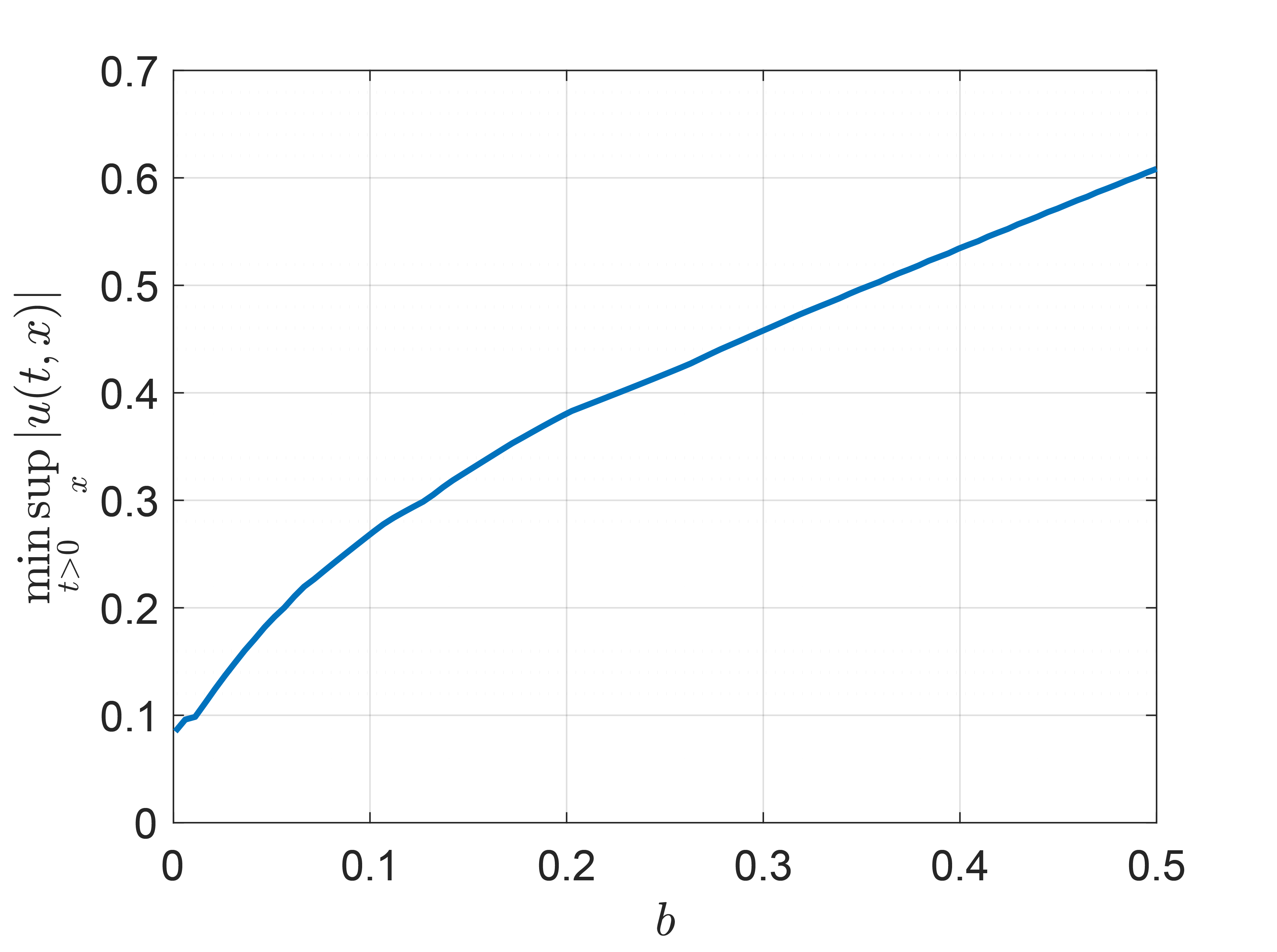
Figure 1. Dependence of $\mathrm{m}$ as defined in (5.39) on $b$ for $u(t,x)$ given by (5.41) where $n=100$, $z=1$, ${0\leq t\leq 2\pi}$, ${-\pi\leq x\leq\pi}$, and using $N=2500$ grid points each for $x$ and $t$ (i.e., $\Delta t=\Delta x\approx 2.5\times 10^{-3}$). The simulations consider $100$ $b$-values in the range $10^{-3}\leq b\leq 5\times 10^{-1}$ with $\Delta b\approx 5\times 10^{-3}$.

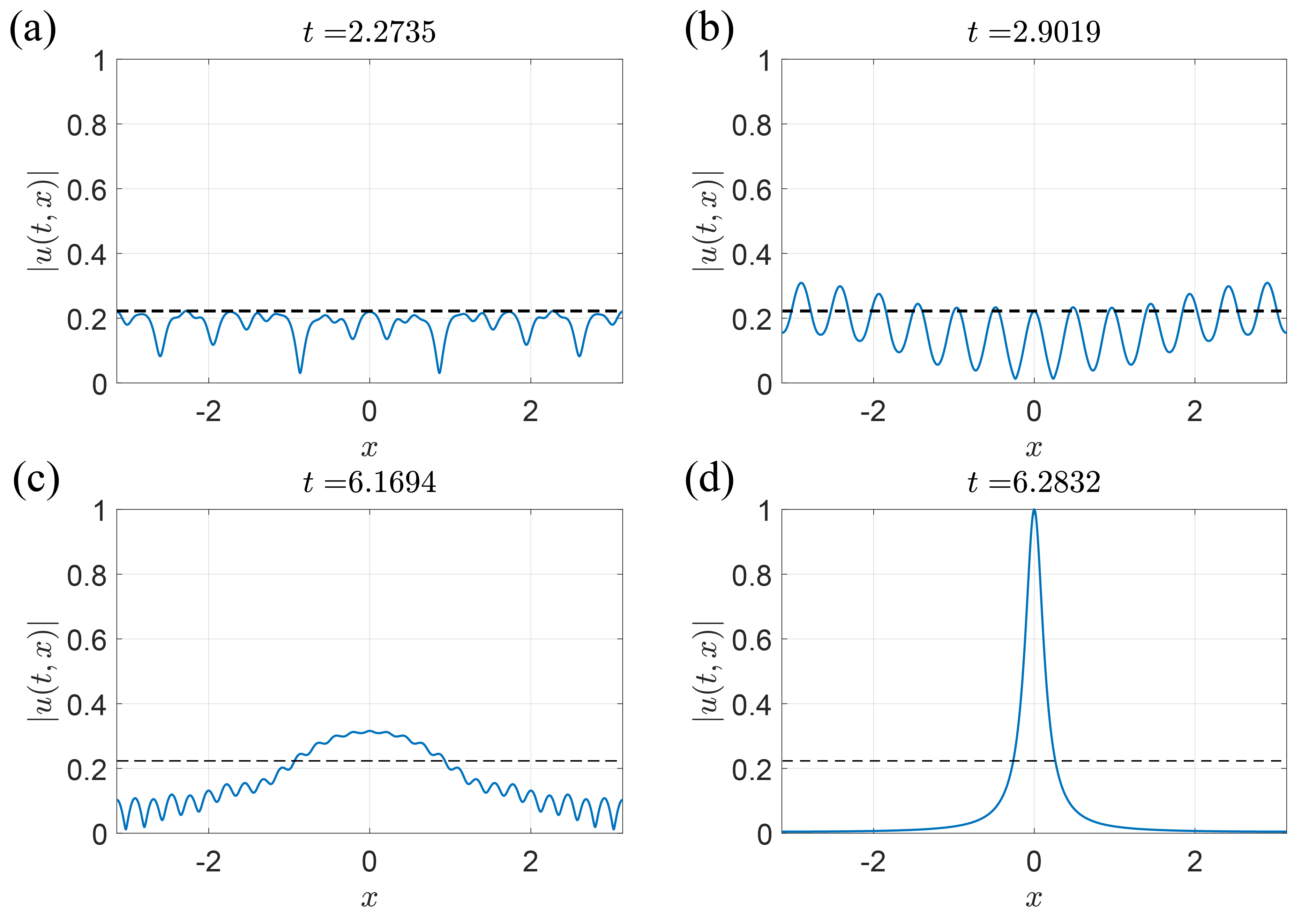
Figure 2. Snapshots of numerical simulations of (5.41) at times: (a) $t\approx 2.2735$, (b) $t\approx 2.9019$, (c) $t\approx 6.1694$, and (d) $t\approx 6.2832$. The solution was simulated for ${0\leq t\leq 2\pi}$, ${-\pi\leq x\leq\pi}$ using $z=1$, $b=0.07$, $n=100$, and $N=10^{4}$ grid points each for $x$ and $t$ (i.e., $\Delta t=\Delta x\approx 6.28\times 10^{-4}$). The dashed line in each image represents the value $\displaystyle{\mathrm{m}\approx 0.2225}$ as defined in (5.39), which is obtained in (a).

In this section we investigate the question of maximum possible growth of rogue waves as described in 5.11. The main question is the following: which is the smallest initial datum $\vartheta\in\mathcal{H}$ that gives rise to a rogue wave of height $z>0$ at time $t_{0}>0$. This smallness is measured in terms of the initial height: $\sup_{x\in\mathbb{T}}|u(0,x\,|\,\vartheta)|$.

In the case of the linear Schrödinger equation, we focus on the minimizers obtained in 5.1. Using the symmetries of the Schrödinger equation, we may assume that the peak of the rogue wave happens at $x^{\ast}=0$, with phase $\phi_{0}^{\ast}=0$, at time $t=0$. Moreover, we may normalize the height so that $z=1$. This initial datum is given by

(5.38) $$u_{0}^{\ast}(x)=\sum_{k\in\mathbb{Z}}\frac{c_{k}^{2}}{\sum_{j\in\mathbb{Z}}c_{j}^{2}}\,e^{ikx}.$$

Then the question of maximum possible growth is equivalent to finding the following quantity:

(5.39) $$\mathrm{m}=\min_{t\geq 0}\sup_{x\in\mathbb{T}}|u(t,x)|.$$

We conduct numerical simulations to find (5.39) in the case where $u(t,x)$ is the solution to the linear Schrödinger equation with initial datum (5.38). To do so, we must truncate the series in (5.38), so we consider

(5.40) $$u_{0}^{\ast}(x)=\sum_{|k|\leq n}\frac{c_{k}^{2}}{\sum_{|j|\leq n}c_{j}^{2}}\,e^{ikx}$$

and the associated solution

(5.41) $$u(t,x)=\sum_{|k|\leq n}\frac{c_{k}^{2}}{\sum_{|j|\leq n}c_{j}^{2}}\,e^{ikx-it|k|^{2}}.$$

We were first interested in exploring the dependence of growth on the constant $b$ appearing in the exponent of $c_{k}$ in (1.8). We therefore computed $u(t,x)$ from (5.41) with $n=100$, $-\pi\leq x\leq\pi$, and $0\leq t\leq 2\pi$ using 2500 data points each for $x$ and $t$ (i.e., $\Delta t=\Delta x\approx 2.5\times 10^{-3}$). We then computed $\mathrm{m}$ in (5.39) for $100$ values of $b$ in the range $10^{-3}\leq b\leq 5\times 10^{-1}$ and note that $\mathrm{m}=\mathrm{m}(b)$ generally decreases as $b$ is decreased (Figure 1). Note that Figure 1 seems to break down as $b\to 0^{+}$. We suspect that this is due to the use of $n=100$. Equations (5.14) and (5.16) seem to indicate that one needs to control a certain number of Fourier modes for the truncation error to stay small. This number grows proportionally to $1/b$, so we might expect that for $b\lesssim 0.01$ (up to an unknown constant) this number would need to be larger than 100.

As a demonstration of this growth, we chose $b=0.07$ and used a refined discretization of $\Delta t=\Delta x\approx 6.28\times 10^{-4}$ to capture dynamics on fast time scales. This computation yields $\mathrm{m}\approx 0.2225$, representing a wave whose height can grow by a factor of approximately $4.5$. Snapshots of the simulation are shown in Figure 2. The dashed black line indicates the value of $\mathrm{m}$, which is obtained in Figure 2(a).

References

- [1] Miguel A. Alejo, Luca Fanelli, and Claudio Muñoz, Review on the stability of the peregrine and related breathers, Frontiers in Physics 8 (2020), 404.
- [2] Theodore Wilbur Anderson, An introduction to multivariate statistical analysis, Wiley New York, 1958.
- [3] George E. Andrews, The Theory of Partitions, Encyclopedia of Mathematics and its Applications, Cambridge University Press, 1984.
- [4] M. Berti and A. Maspero, Long time dynamics of Schrödinger and wave equations on flat tori, J. Differential Equations 267 (2019), no. 2, 1167–1200. MR 3957984
- [5] Marco Bertola and Alexander Tovbis, Universality for the focusing nonlinear Schrödinger equation at the gradient catastrophe point: rational breathers and poles of the tritronquée solution to Painlevé I, Comm. Pure Appl. Math. 66 (2013), no. 5, 678–752. MR 3028484
- [6] J. Bourgain, Fourier transform restriction phenomena for certain lattice subsets and applications to nonlinear evolution equations. I. Schrödinger equations, Geom. Funct. Anal. 3 (1993), no. 2, 107–156. MR 1209299
- [7] by same author, Periodic nonlinear Schrödinger equation and invariant measures, Comm. Math. Phys. 166 (1994), no. 1, 1–26. MR 1309539
- [8] by same author, Invariant measures for the D-defocusing nonlinear Schrödinger equation, Comm. Math. Phys. 176 (1996), no. 2, 421–445. MR 1374420
- [9] by same author, Global wellposedness of defocusing critical nonlinear Schrödinger equation in the radial case, J. Amer. Math. Soc. 12 (1999), no. 1, 145–171. MR 1626257
- [10] by same author, Growth of Sobolev norms in linear Schrödinger equations with quasi-periodic potential, Comm. Math. Phys. 204 (1999), no. 1, 207–247. MR 1705671
- [11] T. Buckmaster, P. Germain, Z. Hani, and J. Shatah, Onset of the wave turbulence description of the longtime behavior of the nonlinear Schrödinger equation, Invent. Math. 225 (2021), no. 3, 787–855. MR 4296350
- [12] Rémi Carles, Eric Dumas, and Christof Sparber, Multiphase weakly nonlinear geometric optics for Schrödinger equations, SIAM J. Math. Anal. 42 (2010), no. 1, 489–518. MR 2607351
- [13] Rémi Carles and Erwan Faou, Energy cascades for NLS on the torus, Discrete Contin. Dyn. Syst. 32 (2012), no. 6, 2063–2077. MR 2885798
- [14] Thierry Cazenave and Fred B. Weissler, The Cauchy problem for the nonlinear Schrödinger equation in , Manuscripta Math. 61 (1988), no. 4, 477–494. MR 952091
- [15] J. Colliander, M. Keel, G. Staffilani, H. Takaoka, and T. Tao, Global well-posedness and scattering for the energy-critical nonlinear Schrödinger equation in , Ann. of Math. (2) 167 (2008), no. 3, 767–865. MR 2415387
- [16] by same author, Transfer of energy to high frequencies in the cubic defocusing nonlinear Schrödinger equation, Invent. Math. 181 (2010), no. 1, 39–113. MR 2651381
- [17] J. Colliander, G. Simpson, and C. Sulem, Numerical simulations of the energy-supercritical nonlinear Schrödinger equation, J. Hyperbolic Differ. Equ. 7 (2010), no. 2, 279–296. MR 2659737
- [18] Charles Collot and Pierre Germain, On the derivation of the homogeneous kinetic wave equation, 2019, preprint.
- [19] by same author, Derivation of the homogeneous kinetic wave equation: longer time scales, 2020, preprint.
- [20] Giuseppe Da Prato, An introduction to infinite-dimensional analysis, Springer Science & Business Media, 2006.
- [21] Giovanni Dematteis, Tobias Grafke, Miguel Onorato, and Eric Vanden-Eijnden, Experimental evidence of hydrodynamic instantons: The universal route to rogue waves, Phys. Rev. X 9 (2019), 041057.
- [22] Giovanni Dematteis, Tobias Grafke, and Eric Vanden-Eijnden, Rogue waves and large deviations in deep sea, Proc. Natl. Acad. Sci. USA 115 (2018), no. 5, 855–860. MR 3763700
- [23] by same author, Extreme event quantification in dynamical systems with random components, SIAM/ASA J. Uncertain. Quantif. 7 (2019), no. 3, 1029–1059. MR 3992060
- [24] Amir Dembo and Ofer Zeitouni, Large deviations techniques and applications, Stochastic Modelling and Applied Probability, vol. 38, Springer, Berlin, Heidelberg, 2011.
- [25] Yu Deng, On growth of Sobolev norms for energy critical NLS on irrational tori: small energy case, Comm. Pure Appl. Math. 72 (2019), no. 4, 801–834. MR 3914883
- [26] Yu Deng and Pierre Germain, Growth of solutions to NLS on irrational tori, Int. Math. Res. Not. IMRN (2019), no. 9, 2919–2950. MR 3947642
- [27] Yu Deng and Zaher Hani, Full derivation of the wave kinetic equation, 2021, preprint.
- [28] Yu Deng and Zaher Hani, On the derivation of the wave kinetic equation for NLS, Forum of Mathematics, Pi 9 (2021), e6.
- [29] Yu Deng, Andrea R. Nahmod, and Haitian Yue, Invariant gibbs measures and global strong solutions for nonlinear schrödinger equations in dimension two, 2019, preprint.
- [30] by same author, Random tensors, propagation of randomness, and nonlinear dispersive equations, 2020, Inventiones Mathematicae, to appear.
- [31] Benjamin Dodson, Global well-posedness and scattering for the defocusing, -critical, nonlinear Schrödinger equation when , Duke Math. J. 165 (2016), no. 18, 3435–3516. MR 3577369
- [32] Benjamin Dodson, Jonas Lührmann, and Dana Mendelson, Almost sure local well-posedness and scattering for the 4D cubic nonlinear Schrödinger equation, Adv. Math. 347 (2019), 619–676. MR 3920835
- [33] K. B. Dysthe, Note on a modification to the nonlinear Schrödinger equation for application to deep water waves, Proc. R. Soc. Lond. A 369 (1979), 105–114.
- [34] Kristian Dysthe, Harald E. Krogstad, and Peter Müller, Oceanic rogue waves, Annual Review of Fluid Mechanics 40 (2008), no. 1, 287–310.
- [35] Mohammad Farazmand and Themistoklis P. Sapsis, Reduced-order prediction of rogue waves in two-dimensional deep-water waves, J. Comput. Phys. 340 (2017), 418–434. MR 3635844
- [36] Igor Rodnianski Frank Merle, Pierre Raphael and Jeremie Szeftel, On blow up for the energy super critical defocusing non linear schrödinger equations, 2019, preprint.
- [37] J. Ginibre and G. Velo, On a class of nonlinear Schrödinger equations. I. The Cauchy problem, general case, J. Functional Analysis 32 (1979), no. 1, 1–32. MR 533218
- [38] Ricardo Grande, Kristin M. Kurianski, and Gigliola Staffilani, On the nonlinear Dysthe equation, Nonlinear Anal. 207 (2021), 112292, 36. MR 4220762
- [39] Manoussos G. Grillakis, On nonlinear Schrödinger equations, Comm. Partial Differential Equations 25 (2000), no. 9-10, 1827–1844. MR 1778782
- [40] Marcel Guardia, Zaher Hani, Emanuele Haus, Alberto Maspero, and Michela Procesi, A note on growth of Sobolev norms near quasiperiodic finite-gap tori for the 2D cubic NLS equation, Atti Accad. Naz. Lincei Rend. Lincei Mat. Appl. 30 (2019), no. 4, 865–880. MR 4030352
- [41] Sebastian Herr, Daniel Tataru, and Nikolay Tzvetkov, Global well-posedness of the energy-critical nonlinear Schrödinger equation with small initial data in , Duke Math. J. 159 (2011), no. 2, 329–349. MR 2824485
- [42] Alexander Hrabski and Yulin Pan, Effect of discrete resonant manifold structure on discrete wave turbulence, Phys. Rev. E 102 (2020), no. 4, 041101(R), 5. MR 4174182
- [43] Alexander Hrabski, Yulin Pan, Gigliola Staffilani, and Bobby Wilson, Energy transfer for solutions to the nonlinear Schrödinger equation on irrational tori, arXiv:2107.01459 (2021).
- [44] Alexandru D. Ionescu and Benoit Pausader, The energy-critical defocusing NLS on , Duke Math. J. 161 (2012), no. 8, 1581–1612. MR 2931275
- [45] Tosio Kato, On nonlinear Schrödinger equations, Ann. Inst. H. Poincaré Phys. Théor. 46 (1987), no. 1, 113–129. MR 877998
- [46] Joel L. Lebowitz, Harvey A. Rose, and Eugene R. Speer, Statistical mechanics of the nonlinear Schrödinger equation, J. Statist. Phys. 50 (1988), no. 3-4, 657–687. MR 939505
- [47] Georg Lindgren, Some properties of a normal process near a local maximum, The Annals of Mathematical Statistics 41 (1970), no. 6, 1870–1883.
- [48] by same author, Extreme values of stationary normal processes, Zeitschrift für Wahrscheinlichkeitstheorie und Verwandte Gebiete 17 (1971), no. 1, 39–47.
- [49] by same author, Local maxima of Gaussian fields, Ark. Mat. 10 (1972), 195–218. MR 319259
- [50] by same author, Wave-length and amplitude for a stationary Gaussian process after a high maximum, Z. Wahrscheinlichkeitstheorie und Verw. Gebiete 23 (1972), 293–326. MR 321169
- [51] A. J. Majda, D. W. McLaughlin, and E. G. Tabak, A one-dimensional model for dispersive wave turbulence, J. Nonlinear Sci. 7 (1997), no. 1, 9–44. MR 1431687
- [52] Frank Merle and Pierre Raphael, The blow-up dynamic and upper bound on the blow-up rate for critical nonlinear Schrödinger equation, Ann. of Math. (2) 161 (2005), no. 1, 157–222. MR 2150386
- [53] Razvan Mosincat, Didier Pilod, and Jean-Claude Saut, Global well-posedness and scattering for the Dysthe equation in , J. Math. Pures Appl. (9) 149 (2021), 73–97. MR 4238997
- [54] M. Onorato, S. Residori, U. Bortolozzo, A. Montina, and F. T. Arecchi, Rogue waves and their generating mechanisms in different physical contexts, Phys. Rep. 528 (2013), no. 2, 47–89. MR 3070399
- [55] Fabrice Planchon, Nikolay Tzvetkov, and Nicola Visciglia, On the growth of Sobolev norms for NLS on 2- and 3-dimensional manifolds, Anal. PDE 10 (2017), no. 5, 1123–1147. MR 3668586
- [56] Mohommed M. Siddiqui, Some problems connected with Rayleigh distributions, Journal of Research of the National Bureau of Standards 66 (1962), 167–174.
- [57] Vedran Sohinger, Bounds on the growth of high Sobolev norms of solutions to nonlinear Schrödinger equations on , Indiana Univ. Math. J. 60 (2011), no. 5, 1487–1516. MR 2996998
- [58] Gigliola Staffilani, On the growth of high Sobolev norms of solutions for KdV and Schrödinger equations, Duke Math. J. 86 (1997), no. 1, 109–142. MR 1427847
- [59] Gigliola Staffilani and Minh-Binh Tran, On the wave turbulence theory for stochastic and random multidimensional KdV type equations, 2021, preprint.
- [60] Gigliola Staffilani and Bobby Wilson, Stability of the cubic nonlinear Schrodinger equation on an irrational torus, SIAM J. Math. Anal. 52 (2020), no. 2, 1318–1342. MR 4078804
- [61] Terence Tao, Monica Visan, and Xiaoyi Zhang, The nonlinear Schrödinger equation with combined power-type nonlinearities, Comm. Partial Differential Equations 32 (2007), no. 7-9, 1281–1343. MR 2354495
- [62] Yoshio Tsutsumi, Global strong solutions for nonlinear Schrödinger equations, Nonlinear Anal. 11 (1987), no. 10, 1143–1154. MR 913674
- [63] Monica Visan, The defocusing energy-critical nonlinear Schrödinger equation in higher dimensions, Duke Math. J. 138 (2007), no. 2, 281–374. MR 2318286
- [64] Xueying Yu, Global well-posedness and scattering for the defocusing -critical nonlinear Schrödinger equation in , arXiv:1805.03230.
- [65] Haitian Yue, Global well-posedness for the energy-critical focusing nonlinear Schrödinger equation on , J. Differential Equations 280 (2021), 754–804. MR 4211014