Shortest Beer Path Queries in Outerplanar Graphs

Abstract

A beer graph is an undirected graph $G$, in which each edge has a positive weight and some vertices have a beer store. A beer path between two vertices $u$ and $v$ in $G$ is any path in $G$ between $u$ and $v$ that visits at least one beer store.

We show that any outerplanar beer graph $G$ with $n$ vertices can be preprocessed in $O(n)$ time into a data structure of size $O(n)$, such that for any two query vertices $u$ and $v$, (i) the weight of the shortest beer path between $u$ and $v$ can be reported in $O(\alpha(n))$ time (where $\alpha(n)$ is the inverse Ackermann function), and (ii) the shortest beer path between $u$ and $v$ can be reported in $O(L)$ time, where $L$ is the number of vertices on this path. Both results are optimal, even when $G$ is a beer tree (i.e., a beer graph whose underlying graph is a tree).

1 Introduction

Imagine that you are going to visit a friend and, not wanting to show up empty handed, you decide to pick up some beer along the way. In this paper we determine the fastest way to go from your place to your friend’s place while stopping at a beer store to buy some drinks.

A beer graph is a undirected graph $G=(V,E)$, in which each edge $(u,v)$ has a positive weight $\omega(u,v)$ and some of the vertices are beer stores. For two vertices $u$ and $v$ of $G$, we define the shortest beer path from $u$ to $v$ to be the shortest (potentially non-simple) path that starts at $u$, ends at $v$, and visits at least one beer store. We denote this shortest path by $\mathsf{SP}_{B}(u,v)$. The beer distance $\mathsf{dist}_{B}(u,v)$ between $u$ and $v$ is the weight of the path $\mathsf{SP}_{B}(u,v)$, i.e., the sum of the edge weights on $\mathsf{SP}_{B}(u,v)$.

Observe that even though the shortest beer path from $u$ to $v$ may be a non-simple path, it is always composed of two simple paths: the shortest path from $u$ to a beer store and the shortest path from this same beer store to $v$. Thus, when looking at the shortest beer path problem, we often need to consider the shortest path between vertices. We denote the shortest path in $G$ from $u$ to $v$ by $\mathsf{SP}(u,v)$ and we use $\mathsf{dist}(u,v)$ to denote the weight of this path. We also say that $\mathsf{dist}(u,v)$ is the distance between $u$ and $v$ in $G$.

To the best of our knowledge, the problem of computing shortest beer paths has not been considered before. Let $s$ be a fixed source vertex of $G$. Recall that Dijkstra’s algorithm computes $\mathsf{dist}(s,v)$ for all vertices $v$, by maintaining a “tentative distance” $\delta(v)$, which is the weight of the shortest path from $s$ to $v$ computed so far. If we also maintain a “tentative beer distance” $\delta_{B}(v)$ (which is the weight of the shortest beer path from $s$ to $v$ that has been found so far), then a modification of Dijkstra’s algorithm allows us to compute $\mathsf{dist}_{B}(s,v)$ for all vertices $v$, in $O(|V|\log|V|+|E|)$ total time.

As far as we know, no non-trivial results are known for beer distance queries. In this case, we want to preprocess the beer graph $G$ into a data structure, such that, for any two query vertices $u$ and $v$, the shortest beer path $\mathsf{SP}_{B}(u,v)$, or its weight $\mathsf{dist}_{B}(u,v)$, can be reported.

1.1 Our Results

We present data structures that can answer shortest beer path queries in outerplanar beer graphs. Recall that a graph $G$ is outerplanar, if $G$ can be embedded in the plane, such that all vertices are on the outer face, and no two edges cross.

Our first result is stated in terms of the inverse Ackermann function. We use the definition as given in [3]: Let $A_{0}(i)=i+1$ and, for $\ell\geq 0$, $A_{\ell+1}(i)=A_{\ell}^{(i+1)}(i+8)$, where $A_{\ell}^{(i+1)}$ is the function $A_{\ell}$ iterated $i+1$ times. We define $\alpha(m,n)$ to be the smallest value of $\ell$ for which $A_{\ell}(\lfloor m/n\rfloor)>n$, and we define $\alpha(n)=\alpha(n,n)$.

Theorem 1

Let $G$ be an outerplanar beer graph with $n$ vertices. For any integer $m\geq n$, we can preprocess $G$ in $O(m)$ time into a data structure of size $O(m)$, such that for any two query vertices $u$ and $v$, both $\mathsf{dist}(u,v)$ and $\mathsf{dist}_{B}(u,v)$ can be computed in $O(\alpha(m,n))$ time.

By taking $m=n$, both the preprocessing time and the space used are $O(n)$, and for any two query vertices $u$ and $v$, both $\mathsf{dist}(u,v)$ and $\mathsf{dist}_{B}(u,v)$ can be computed in $O(\alpha(n))$ time.

As another example, let $\log^{*}n$ be the number of times the function $\log$ must be applied, when starting with the value $n$, until the result is at most $1$, and let $\log^{**}n$ be the number of times the function $\log^{*}$ must be applied, again starting with $n$, until the result is at most $1$. Let $m=n\log^{**}n$. Since $\alpha(m,n)=O(1)$, we obtain a data structure with space and preprocessing time $O(n\log^{**}n)$ that can answer both distance and beer distance queries in $O(1)$ time.

As we mentioned before, beer distance queries have not been considered for any class of graphs. In fact, the only result on (non-beer) distance queries in outerplanar graphs that we are aware of is by Djidjev et al. [5]. They show that an outerplanar graph with $n$ vertices can be preprocessed in $O(n\log n)$ time into a data structure of size $O(n\log n)$, such that any distance query can be answered in $O(\log n)$ time. Our result in Theorem 1 significantly improves their result.

We also show that the result in Theorem 1 is optimal for beer distance queries, even if $G$ is a beer tree (i.e., a beer graph whose underlying graph is a tree). We do not know if the query time is optimal for (non-beer) distance queries.

Our second result is on reporting the shortest beer path between two query vertices.

Theorem 2

Let $G$ be an outerplanar beer graph with $n$ vertices. We can preprocess $G$ in $O(n)$ time into a data structure of size $O(n)$, such that for any two vertices $u$ and $v$, the shortest beer path from $u$ to $v$ can be reported in $O(L)$ time, where $L$ is the number of vertices on this beer path.

Observe that the query time in Theorem 2 does not depend on the number $n$ of vertices of the graph. Again, we are not aware of any previous work on reporting shortest beer paths. Djidjev et al. [5] show that, after $O(n\log n)$ preprocessing and using $O(n\log n)$ space, the shortest (non-beer) path between two query vertices can be reported in $O(\log n+L)$ time, where $L$ is the number of vertices on the path.

1.2 Preliminaries and Organization

Throughout this paper, we only consider outerplanar beer graphs $G$. The number of vertices of $G$ is denoted by $n$. It is well known that $G$ has at most $2n-3$ edges. As in [5], we say that $G$ satisfies the generalized triangle inequality, if for every edge $(u,v)$ in $G$, $\mathsf{dist}(u,v)=\omega(u,v)$, i.e., the shortest path between $u$ and $v$ is the edge $(u,v)$.

The outerplanar graph $G$ is called maximal, if adding an edge between any two non-adjacent vertices of $G$ results in a graph that is not outerplanar. In this case, the number of edges is equal to $2n-3$. A maximal outerplanar graph $G$ is 2-connected, each internal face of $G$ is a triangle and the outer face of $G$ forms a Hamiltonian cycle. In such a graph, edges on the outer face will be referred to as external edges, where all other edges will be referred to as internal edges.

The weak dual of a maximal outerplanar graph $G$ is the graph $D(G)$ whose node set is the set of all internal faces of $G$, and in which $(F,F^{\prime})$ is an edge if and only if the faces $F$ and $F^{\prime}$ share an edge in $G$; see Figure 1. For simplicity, we will refer to $D(G)$ as the dual of $G$. Observe that $D(G)$ is a tree with $n-2$ nodes, each of which has degree at most three.

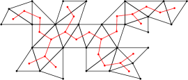
Figure 1: A maximal outerplanar graph shown in black. Its dual is shown in red.

If $H$ is a subgraph of the beer graph $G$, and $u$ and $v$ are vertices of $H$, then $\mathsf{dist}(u,v,H)$ and $\mathsf{dist}_{B}(u,v,H)$ denote the distance and beer distance between $u$ and $v$ in $H$, respectively. The shortest beer path in $H$ between $u$ and $v$ must be entirely within $H$. Observe that we use the shorthand $\mathsf{dist}(u,v)$ for $\mathsf{dist}(u,v,G)$, and $\mathsf{dist}_{B}(u,v)$ for $\mathsf{dist}_{B}(u,v,G)$.

It will not be surprising that the algorithms for computing shortest beer paths use the dual $D(G)$. Thus, our algorithms will need some basic data structures on trees. These data structures will be presented in Section 2.

In Section 3, we will prove Theorem 1 for maximal outerplanar beer graphs. We also prove that the result in Theorem 1 is optimal, even for beer trees. The proof of Theorem 2, again for maximal outerplanar beer graphs, will be presented in Section 4. Both Sections 3 and 4 will use the result in Lemma 4, whose detailed proof will be given in Section 5.

The extensions of Theorems 1 and 2 to arbitrary outerplanar beer graphs will be given in Section 6. Finally, Section 7 will present an $O(n)$-time algorithm for computing the single-source shortest beer path tree for any given source vertex.

2 Query Problems on Trees

Our algorithms for computing beer shortest paths in an outerplanar graph $G$ will use the dual of $G$, which is a tree. In order to obtain fast implementations of these algorithms, we need to be able to solve several query problems on this tree. In this section, we present all query problems that will be used in later sections.

Lemma 1

Let $T$ be a tree with $n$ nodes that is rooted at an arbitrary node. We can preprocess $T$ in $O(n)$ time, such that each of the following queries can be answered in $O(1)$ time:

1. Given a node $u$ of $T$, return its level, denoted by $\mathord{\it level}(u)$, which is the number of edges on the path from $u$ to the root.

2. Given two nodes $u$ and $v$ of $T$, report their lowest common ancestor, denoted by $\mathsf{LCA}(u,v)$.

3. Given two nodes $u$ and $v$ of $T$, decide whether or not $u$ is in the subtree rooted at $v$.

4. Given two distinct nodes $u$ and $v$ of $T$, report the second node on the path from $u$ to $v$.

5. Given three nodes $u$, $v$, and $w$, decide whether or not $w$ is on the path between $u$ and $v$.

Proof. The first claim follows from the fact that by performing an $O(n)$–time pre-order traversal of $T$, we can compute $\mathord{\it level}(u)$ for each node $u$. A proof of the second claim can be found in Harel and Tarjan [6] and Bender and Farach-Colton [2]. The third claim follows from the fact that $u$ is in the subtree rooted at $v$ if and only $\mathsf{LCA}(u,v)=v$. A proof of the fourth claim can be found in Chazelle [4, Lemma 15]. The fifth claim follows from the following observations. Assume that $u$ is in the subtree rooted at $v$. Then $w$ is on the path between $u$ and $v$ if and only if $\mathsf{LCA}(u,w)=w$ and $w$ is in the subtree rooted at $v$. The case when $v$ is in the subtree rooted at $u$ is symmetric. Assume that $\mathsf{LCA}(u,v)\not\in\{u,v\}$. Then $w$ is on the path between $u$ and $v$ if and only if $w$ is on the path between $u$ and $\mathsf{LCA}(u,v)$ or $w$ is on the path between $v$ and $\mathsf{LCA}(u,v)$.   

2.1 Closest-Colour Queries in Trees

Let $T$ be a tree with $n$ nodes and let $\mathcal{C}$ be a set of colours. For each colour $c$ in $\mathcal{C}$, we are given a path $P_{c}$ in $T$. Even though these paths may share nodes, each node of $T$ belongs to at most a constant number of paths. This implies that the total size of all paths $P_{c}$ is $O(n)$. We assume that each node $u$ of $T$ stores the set of all colors $c$ such that $u$ is on the path $P_{c}$.

In a closest-colour query, we are given two nodes $u$ and $v$ of $T$, and a colour $c$, such that $u$ is on the path $P_{c}$. The answer to the query is the node on $P_{c}$ that is closest to $v$. Refer to Figure 2 for an illustration.

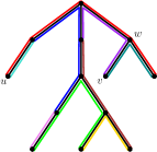
Figure 2: A tree $T$ and a collection of coloured paths. For a query with nodes $u$ and $v$, and color “red”, the answer is the node $w$.

Lemma 2

After an $O(n)$–time preprocessing, we can answer any closest-colour query in $O(1)$ time.

Proof. We take an arbitrary node of $T$ and make it the root. Then we preprocess $T$ such that each of the queries in Lemma 1 can be answered in $O(1)$ time.

For each colour $c$, let $c^{1}$ and $c^{2}$ be the end nodes of the path $P_{c}$, and let $c^{h}$ be the highest node on $P_{c}$ in the tree (i.e., the node on $P_{c}$ that is closest to the root). With each node of $P_{c}$, we store pointers to $c^{1}$, $c^{2}$, and $c^{h}$.

Since each node of $T$ is in a constant number of coloured paths, we can compute the pointers for all the coloured paths in $O(n)$ total time.

The query algorithm does the following. Let $u$ and $v$ be two nodes of $T$, and let $c$ be a colour such that $u$ is on the $c$-coloured path $P_{c}$.

If $u=v$ or $v$ is also on $P_{c}$, then we return the node $v$. From now on, assume that $u\neq v$ and $v$ is not on $P_{c}$. Below, we consider all possible cases, which are illustrated in Figure 3.

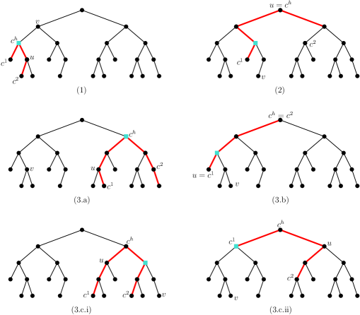
Figure 3: Illustrating all possible cases in the proof of Lemma 2. The path $P_{c}$ is red and the blue square indicates the node that is returned by the closest-colour query.

1. If $\mathsf{LCA}(u,v)=v$, then $u$ is in the subtree rooted at $v$. In this case, we return $c^{h}$, the highest $c$-coloured node.

2. Assume that $\mathsf{LCA}(u,v)=u$. Then $v$ is in the subtree rooted at $u$. The closest $c$-coloured node to $v$ is either $\mathsf{LCA}(v,c^{1})$ or $\mathsf{LCA}(v,c^{2})$. Since $v$ is lower than $u$ in the tree, we know that the closest $c$-colored node to $v$ is at $\mathord{\it level}(u)$ or greater. If $\mathord{\it level}(\mathsf{LCA}(v,c^{1}))>\mathord{\it level}(\mathsf{LCA}(v,c^{2}))$, then $\mathsf{LCA}(v,c^{1})$ is lower in the tree and closer to $v$, so we return $\mathsf{LCA}(v,c^{1})$ . Otherwise, $\mathsf{LCA}(v,c^{2})$ is lower in $T$ or equal to both $\mathsf{LCA}(v,c^{1})$ and $u$, so we return $\mathsf{LCA}(v,c^{2})$.

3. Assume that $\mathsf{LCA}(u,v)\neq u$ and $\mathsf{LCA}(u,v)\neq v$. Then $u$ and $v$ are in different subtrees of $\mathsf{LCA}(u,v)$.

   1. If $\mathord{\it level}(c^{h})>\mathord{\it level}(\mathsf{LCA}(u,v))$, then we return $c^{h}$.

   2. If $\mathord{\it level}(c^{h})<\mathord{\it level}(\mathsf{LCA}(u,v))$, then we return $\mathsf{LCA}(u,v)$.

   3. Assume that $\mathord{\it level}(c^{h})=\mathord{\it level}(\mathsf{LCA}(u,v))$. Observe that exactly one end node of the $c$-coloured path is in the subtree rooted at $u$.

      1. If $c^{1}$ is in the subtree rooted at $u$, then we return $\mathsf{LCA}(v,c^{2})$.

      2. If $c^{2}$ is in the subtree rooted at $u$, then we return $\mathsf{LCA}(v,c^{1})$.

Using Lemma 1, each of these case takes $O(1)$ time. Therefore, the entire query algorithm takes $O(1)$ time.   

2.2 Path-Sum Queries in Trees

Let $(W,\oplus)$ be a semigroup. Thus, $W$ is a set and $\oplus:W\times W\rightarrow W$ is an associative binary operator. We assume that for any two elements $s$ and $s^{\prime}$ in $W$, the value of $s\oplus s^{\prime}$ can be computed in $O(1)$ time.

Let $T$ be a tree with $n$ nodes in which each edge $e$ stores a value $s(e)$, which is an element of $W$. For any two distinct nodes $u$ and $v$ in $T$, we define their path-sum $\mathsf{PS}(u,v)$ as follows: Let $e_{1},e_{2},\ldots,e_{k}$ be the edges on the path in $T$ between $u$ and $v$. Then we define $\mathsf{PS}(u,v)=\oplus_{i=1}^{k}s(e_{i})$.

Chazelle [4] considers the problem of preprocessing the tree $T$, such that for any two distinct query nodes $u$ and $v$, the value of $\mathsf{PS}(u,v)$ can be reported. (See also Alon and Schieber [1], Thorup [9], and Chan et al. [3].) Chazelle’s result is stated in terms of the inverse Ackermann function; see Section 1.1.

Lemma 3

Let $T$ be a tree with $n$ nodes in which each edge stores an element of the semigroup $(W,\oplus)$. For any integer $m\geq n$, we can preprocess $T$ in $O(m)$ time into a data structure of size $O(m)$, such that any path-sum query can be answered in $O(\alpha(m,n))$ time.

Remark 1

Assume that $(W,\oplus)$ is the semigroup, where $W$ is the set of all real numbers and the operator $\oplus$ takes the minimum of its arguments. In this case, we will refer to a query as a path-minimum query. For this semigroup, the result of Lemma 3 is optimal: Any data structure that can be constructed in $O(m)$ time has worst-case query time $\Omega(\alpha(m,n))$. To prove this, assume that we can answer any query in $o(\alpha(m,n))$ time. Then the on-line minimum spanning tree verification problem on a tree with $n$ vertices and $m\geq n$ queries can be solved in $o(m\cdot\alpha(m,n))$ time, by performing a path-maximum query for the endpoints of each edge $e$ and checking that the weight of $e$ is larger than the path-maximum. This contradicts the lower bound for this problem proved by Pettie [8].

3 Beer Distance Queries in Maximal Outerplanar Graphs

Let $G$ be a maximal outerplanar beer graph with $n$ vertices that satisfies the generalized triangle inequality. We will show how to preprocess $G$, such that for any two vertices $u$ and $v$, the weight, $\mathsf{dist}_{B}(u,v)$, of a shortest beer path between $u$ and $v$ can be reported. Our approach will be to define a special semigroup $(W,\oplus)$, such that each element of $W$ “contains” certain distances and beer distances. With each edge of the dual $D(G)$, we will store one element of the set $W$. As we will see later, a beer distance query can then be reduced to a path-sum query in $D(G)$. Thus, by applying the results of Section 2.2, we will obtain a proof of Theorem 1.

We will need the first claim in the following lemma. The second claim will be used in Section 4.

Lemma 4

Consider the beer graph $G$ as above.

1. In $O(n)$ total time, we can compute $\mathsf{dist}_{B}(u,u)$ for each vertex $u$ of $G$, and $\mathsf{dist}_{B}(u,v)$ for each edge $(u,v)$ in $G$.

2. After an $O(n)$–time preprocessing of $G$, we can report,

   1. for any query edge $(u,v)$ of $G$, the shortest beer path between $u$ and $v$ in $O(L)$ time, where $L$ is the number of vertices on this path,

   2. for any query vertex $u$ of $G$, the shortest beer path from $u$ to itself in $O(L)$ time, where $L$ is the number of vertices on this path.

Proof. We choose an arbitrary face $R$ of $G$ and make it the root of $D(G)$. Let $(u,v)$ be any edge of $G$. This edge divides $G$ into two outerplanar subgraphs, both of which contain $(u,v)$ as an edge. Let $G_{uv}^{R}$ be the subgraph that contains the face $R$, and let $G_{uv}^{\neg R}$ denote the other subgraph. Note that if $(u,v)$ is an external edge, then $G_{uv}^{R}=G$ and $G_{uv}^{\neg R}$ consists of the single edge $(u,v)$. By the generalized triangle inequality, the shortest beer path between $u$ and $v$ is completely in $G_{uv}^{R}$ or completely in $G_{uv}^{\neg R}$. The same is true for the shortest beer path from $u$ to itself. Thus, for each edge $(u,v)$ of $G$,

$$\mathsf{dist}_{B}(u,v)=\min\left(\mathsf{dist}_{B}(u,v,G_{uv}^{R}),\mathsf{dist}_{B}(u,v,G_{uv}^{\neg R})\right),$$

$$\mathsf{dist}_{B}(u,u)=\min\left(\mathsf{dist}_{B}(u,u,G_{uv}^{R}),\mathsf{dist}_{B}(u,u,G_{uv}^{\neg R})\right).$$

By performing a post-order traversal of $D(G)$, we can compute $\mathsf{dist}_{B}(u,v,G_{uv}^{\neg R})$ and $\mathsf{dist}_{B}(u,u,G_{uv}^{\neg R})$ for all edges $(u,v)$, in $O(n)$ total time. After these values have been computed, we perform a pre-order traversal of $D(G)$ and obtain $\mathsf{dist}_{B}(u,v,G_{uv}^{R})$ and $\mathsf{dist}_{B}(u,u,G_{uv}^{R})$, again for all edges $(u,v)$, in $O(n)$ total time. The details will be given in Section 5.   

In the rest of this section, we assume that all beer distances in the first claim of Lemma 4 have been computed.

For any two distinct internal faces $F$ and $F^{\prime}$ of $G$, let $Q_{F,F^{\prime}}$ be the union of the two sets

$$\{(u,v,\mathsf{dist}(u,v),\mathsf{D})\mid u\mbox{ is a vertex of }F,v\mbox{ is a vertex of }F^{\prime}\}$$

and

$$\{(u,v,\mathsf{dist}_{B}(u,v),\mathsf{BD})\mid u\mbox{ is a vertex of }F,v\mbox{ is a vertex of }F^{\prime}\},$$

where the “bits” $\mathsf{D}$ and $\mathsf{BD}$ indicate whether the tuple represents a distance or a beer distance. In words, $Q_{F,F^{\prime}}$ is the set of all shortest path distances and all shortest beer distances between a vertex in $F$ and a vertex in $F^{\prime}$. Since each internal face has three vertices, the set $Q_{F,F^{\prime}}$ has exactly $18$ elements.

Observation 1

Let $u$ and $v$ be vertices of $G$, and let $F$ and $F^{\prime}$ be internal faces that contain $u$ and $v$ as vertices, respectively.

1. If $F=F^{\prime}$, then we can determine both $\mathsf{dist}(u,v)$ and $\mathsf{dist}_{B}(u,v)$ in $O(1)$ time.

2. If $F\neq F^{\prime}$ and we are given the set $Q_{F,F^{\prime}}$, then we can determine both $\mathsf{dist}(u,v)$ and $\mathsf{dist}_{B}(u,v)$ in $O(1)$ time.

Proof. First assume that $F=F^{\prime}$. If $u=v$, then $\mathsf{dist}(u,v)=0$ and $\mathsf{dist}_{B}(u,v)$ has been precomputed. If $u\neq v$, then $(u,v)$ is an edge of $G$ and, thus, $\mathsf{dist}(u,v)=\omega(u,v)$ and $\mathsf{dist}_{B}(u,v)$ has been precomputed.

Assume that $F\neq F^{\prime}$. If we know the set $Q_{F,F^{\prime}}$, then we can find $\mathsf{dist}(u,v)$ and $\mathsf{dist}_{B}(u,v)$ in $O(1)$ time, because these two distances are in $Q_{F,F^{\prime}}$.   

In the rest of this section, we will show that Lemma 3 can be used to compute the set $Q_{F,F^{\prime}}$ for any two distinct internal faces $F$ and $F^{\prime}$.

Lemma 5

For any edge $(F,F^{\prime})$ of $D(G)$, the set $Q_{F,F^{\prime}}$ can be computed in $O(1)$ time.

Proof. Let $u$ be a vertex of $F$ and let $v$ be a vertex of $F^{\prime}$. Consider the subgraph $G[F,F^{\prime}]$ of $G$ that is induced by the four vertices of $F$ and $F^{\prime}$; this subgraph has five edges. By the generalized triangle inequality, $\mathsf{dist}(u,v)=\mathsf{dist}(u,v,G[F,F^{\prime}])$. Thus, $\mathsf{dist}(u,v)$ can be computed in $O(1)$ time.

We now show how $\mathsf{dist}_{B}(u,v)$ can be computed in $O(1)$ time. If $u=v$ or $(u,v)$ is an edge of $G$, then $\mathsf{dist}_{B}(u,v)$ has been precomputed. Assume that $u\neq v$ and $(u,v)$ is not an edge of $G$. Let $w$ and $w^{\prime}$ be the two vertices that are shared by $F$ and $F^{\prime}$. Since any path in $G$ between $u$ and $v$ contains at least one of $w$ and $w^{\prime}$, $\mathsf{dist}_{B}(u,v)$ is the minimum of

1. $\mathsf{dist}_{B}(u,w)+\omega(w,v)$,

2. $\omega(u,w)+\mathsf{dist}_{B}(w,v)$,

3. $\mathsf{dist}_{B}(u,w^{\prime})+\omega(w^{\prime},v)$,

4. $\omega(u,w^{\prime})+\mathsf{dist}_{B}(w^{\prime},v)$.

Since $(u,w)$, $(w,v)$, $(u,w^{\prime})$, and $(w^{\prime},v)$ are edges of $G$, all terms in these four sums have been precomputed. Therefore, $\mathsf{dist}_{B}(u,v)$ can be computed in $O(1)$ time.

We have shown that each of the $18$ elements of $Q_{F,F^{\prime}}$ can be computed in $O(1)$ time. Therefore, this entire set can be computed in $O(1)$ time.   

Lemma 6

Let $F$, $F^{\prime}$, and $F^{\prime\prime}$ be three pairwise distinct internal faces of $G$, such that $F^{\prime}$ is on the path in $D(G)$ between $F$ and $F^{\prime\prime}$. If we are given the sets $Q_{F,F^{\prime}}$ and $Q_{F^{\prime},F^{\prime\prime}}$, then the set $Q_{F,F^{\prime\prime}}$ can be computed in $O(1)$ time.

Proof. Let $u$ be a vertex of $F$ and let $v$ be a vertex of $F^{\prime\prime}$. Since $G$ is an outerplanar graph, any path in $G$ between $u$ and $v$ must contain at least one vertex of $F^{\prime}$. It follows that

$$\mathsf{dist}(u,v)=\min\{\mathsf{dist}(u,w)+\mathsf{dist}(w,v)\mid w\mbox{ is a vertex of }F^{\prime}\}.$$

Thus, since $(u,w,\mathsf{dist}(u,w),\mathsf{D})\in Q_{F,F^{\prime}}$ and $(w,v,\mathsf{dist}(w,v),\mathsf{D})\in Q_{F^{\prime},F^{\prime\prime}}$, the value of $\mathsf{dist}(u,v)$ can be computed in $O(1)$ time.

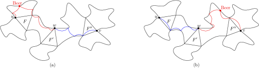
Figure 4: Any beer path from $u$ to $v$ contains at least one vertex of $F^{\prime}$. In (a), we consider the shortest beer path from $u$ to $w$, followed by the shortest path from $w$ to $v$. In (b), we consider the shortest path from $u$ to $w$, followed by the shortest beer path from $w$ to $v$.

By a similar argument, $\mathsf{dist}_{B}(u,v)$ is equal to (refer to Figure 4)

$$\min\{\min(\mathsf{dist}_{B}(u,w)+\mathsf{dist}(w,v),\mathsf{dist}(u,w)+\mathsf{dist}_{B}(w,v)):\mbox{ $w$ is a vertex of $F^{\prime}$}\}.$$

All values $\mathsf{dist}(u,w)$, $\mathsf{dist}(w,v)$, $\mathsf{dist}_{B}(u,w)$, and $\mathsf{dist}_{B}(w,v)$ are encoded in the sets $Q_{F,F^{\prime}}$ and $Q_{F^{\prime},F^{\prime\prime}}$. Therefore, we can compute $\mathsf{dist}_{B}(u,v)$ in $O(1)$ time.

Thus, since each of the $18$ elements of $Q_{F,F^{\prime\prime}}$ can be computed in $O(1)$ time, the entire set can be computed in $O(1)$ time.   

We define

$$W=\{Q_{F,F^{\prime}}\mid\mbox{ $F$ and $F^{\prime}$ are distinct internal faces of $G$}\}\cup\{\bot\},$$

where $\bot$ is a special symbol. We define the operator $\oplus:W\times W\rightarrow W$ in the following way.

1. If $F$ and $F^{\prime}$ are distinct internal faces of $G$, then $Q_{F,F^{\prime}}\oplus Q_{F,F^{\prime}}=Q_{F,F^{\prime}}$.

2. If $F$, $F^{\prime}$, and $F^{\prime\prime}$ are pairwise distinct internal faces of $G$ such that $F^{\prime}$ is on the path in $D(G)$ between $F$ and $F^{\prime\prime}$, then $Q_{F,F^{\prime}}\oplus Q_{F^{\prime},F^{\prime\prime}}=Q_{F,F^{\prime\prime}}$.

3. In all other cases, the operator $\oplus$ returns $\bot$.

It is not difficult to verify that $\oplus$ is associative, implying that $(W,\oplus)$ is a semigroup. By Lemma 5, we can compute $Q_{F,F^{\prime}}$ for all edges $(F,F^{\prime})$ of $D(G)$, in $O(n)$ total time.

Recall from Lemma 1 that, after an $O(n)$–time preprocessing, we can decide in $O(1)$ time, for any three internal faces $F$, $F^{\prime}$, and $F^{\prime\prime}$ of $G$, whether $F^{\prime}$ is on the path in $D(G)$ between $F$ and $F^{\prime\prime}$. Therefore, using Lemma 6, the operator $\oplus$ takes $O(1)$ time to evaluate for any two elements of $W$.

Finally, let $F$ and $F^{\prime}$ be two distinct internal faces of $G$, and let $F=F_{0},F_{1},F_{2},\ldots,F_{k}=F^{\prime}$ be the path in $D(G)$ between $F$ and $F^{\prime}$. Then $Q_{F,F^{\prime}}=\oplus_{i=0}^{k-1}Q_{F_{i},F_{i+1}}$. Thus, if we store with each edge of the tree $D(G)$, the corresponding element of the semigroup, then computing $Q_{F,F^{\prime}}$ becomes a path-sum query as in Section 2.2.

To summarize, all conditions to apply Lemma 3 are satisfied. As a result, we have proved Theorem 1 for maximal outerplanar graphs that satisfy the generalized triangle inequality.

3.1 The Result in Theorem 1 is Optimal

In Section 2.2, see also Remark 1, we have seen path-minimum queries in a tree, in which each edge $e$ stores a real number $s(e)$. In such a query, we are given two distinct nodes $u$ and $v$, and have to return the smallest value $s(e)$ among all edges $e$ on the path between $u$ and $v$. Lemma 3 gives a trade-off between the preprocessing and query times when answering such queries.

Let $D$ be an arbitrary data structure that answers beer distance queries in any beer tree. Let $P(n)$, $S(n)$, and $Q(n)$ denote the preprocessing time, space, and query time of $D$, respectively, when the beer tree has $n$ nodes. We will show that $D$ can be used to answer path-minimum queries.

Consider an arbitrary tree $T$ with $n$ nodes, such that each edge $e$ stores a real number $s(e)$. We may assume without loss of generality that $0<s(e)<1$ for each edge $e$ of $T$.

By making an arbitrary node the root of $T$, the number of edges on the path in $T$ between two nodes $u$ and $v$ is equal to

$$\mathord{\it level}(u)+\mathord{\it level}(v)-2\cdot\mathord{\it level}(\mathsf{LCA}(u,v)).$$

Thus, by Lemma 1, after an $O(n)$–time preprocessing, we can compute the number of edges on this path in $O(1)$ time.

We create a beer tree $T^{\prime}$ as follows. Initially, $T^{\prime}$ is a copy of $T$. For each edge $e=(u,v)$ of $T^{\prime}$, we introduce a new node $x_{e}$ and replace $e$ by two edges $(u,x_{e})$ and $(v,x_{e})$; we assign a weight of $1$ to each of these two edges. In the current tree $T^{\prime}$, none of the nodes has a beer store. For every node $x_{e}$ in $T^{\prime}$, we introduce a new node $x^{\prime}_{e}$, add the edge $(x_{e},x^{\prime}_{e})$, assign a weight of $s(e)$ to this edge, and make $x^{\prime}_{e}$ a beer store. Finally, we construct the data structure $D$ for the resulting beer tree $T^{\prime}$. Since $T^{\prime}$ has $n+2(n-1)=3n-2$ nodes, it takes $P(3n-2)+O(n)$ time to construct $D$ from the input tree $T$. Moreover, the amount of space used is $S(3n-2)+O(n)$.

Let $u$ and $v$ be two distinct nodes in the original tree $T$, let $\pi$ be the path in $T$ between $u$ and $v$, and let $\ell$ be the number of edges on $\pi$. The corresponding path $\pi^{\prime}$ in $T^{\prime}$ between $u$ and $v$ has weight $2\ell$.

For any edge $e$ of $T$, let $\pi^{\prime}_{e}$ be the beer path in $T^{\prime}$ that starts at $u$, goes to $x_{e}$, then goes to $x^{\prime}_{e}$ and back to $x_{e}$, and continues to $v$.

If $e$ is an edge of $\pi$, then the weight of $\pi^{\prime}_{e}$ is equal to $2\ell+2\cdot s(e)$, which is less than $2\ell+2$. On the other hand, if $e$ is an edge of $T$ that is not on $\pi$, then the weight of $\pi^{\prime}_{e}$ is at least $2\ell+2+2\cdot s(e)$, which is larger than $2\ell+2$. It follows that the shortest beer path in $T^{\prime}$ between $u$ and $v$ visits the beer store $x^{\prime}_{e}$, where $e$ is the edge on $\pi$ for which $s(e)$ is minimum.

Thus, by computing $\ell$ and querying $D$ for the beer distance in $T^{\prime}$ between $u$ and $v$, we obtain the smallest value $s(e)$ among all edges $e$ on the path in $T$ between $u$ and $v$. The query time is $Q(3n-2)+O(1)$.

By combining this reduction with Remark 1, it follows that the result of Theorem 1 is optimal.

4 Reporting Shortest Beer Paths in Maximal Outerplanar Graphs

Let $G$ be a maximal outerplanar beer graph with $n$ vertices that satisfies the generalized triangle inequality. In this section, we show that, after an $O(n)$–time preprocessing, we can report, for any two query vertices $s$ and $t$, the shortest beer path $\mathsf{SP}_{B}(s,t)$ from $s$ to $t$, in $O(L)$ time, where $L$ is the number of vertices on this path. As before, $D(G)$ denotes the dual of $G$.

Observation 2

Let $v$ be a vertex of $G$. The faces of $G$ containing $v$ form a path of nodes in $D(G)$.

Define $P_{v}$ to be the path in $D(G)$ formed by the faces of $G$ containing the vertex $v$. Let $G[P_{v}]$ be the subgraph of $G$ induced by the faces of $G$ containing $v$. Note that $G[P_{v}]$ has a fan shape. Let $\mathsf{CW}(v)$ denote the clockwise neighbor of $v$ in $G[P_{v}]$ and let $\mathsf{CCW}(v)$ denote the counterclockwise neighbor of $v$ in $G[P_{v}]$. We will refer to the clockwise path from $\mathsf{CW}(v)$ to $\mathsf{CCW}(v)$ in $G[P_{v}]$ as the $v$-chain and denote it by $\rho_{v}$. (Refer to Figure 5.)

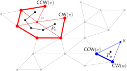
Figure 5: A maximal outerplanar graph $G$. The subgraphs $G[P_{v}]$ and $G[P_{u}]$ are shown in red and blue, respectively. Both the $v$-chain $\rho_{v}$ and the $u$-chain $\rho_{u}$ are shown in bold. Both paths $P_{v}$ and $P_{u}$ are shown in black. Observe that $P_{u}$ is a single node.

Lemma 7

After an $O(n)$–time preprocessing, we can answer the following queries, for any three query vertices $v$, $u$, and $w$, such that both $u$ and $w$ are on the $v$-chain $\rho_{v}$:

1. Report the weight $\mathsf{dist}(u,w,\rho_{v})$ of the path from $u$ to $w$ along $\rho_{v}$ in $O(1)$ time.

2. Report the path $\mathsf{SP}(u,w,\rho_{v})$ from $u$ to $w$ along $\rho_{v}$ in $O(L)$ time, where $L$ is the number of vertices on this path.

Proof. For any vertex $v$ and any vertex $u$ on $\rho_{v}$, we store the weight of the path from $u$ to $\mathsf{CW}(v)$ along $\rho_{v}$. Observe that

$$\mathsf{dist}(u,w,\rho_{v})=|\mathsf{dist}(u,\mathsf{CW}(v),\rho_{v})-\mathsf{dist}(w,\mathsf{CW}(v),\rho_{v})|.$$

Any exterior edge in $G$ is in exactly one chain and any interior edge in $G$ is in exactly two chains. Thus, the sum of the number of edges on each chain is proportional to the number of edges of $G$, which is $O(n)$.   

Lemma 8

After an $O(n)$–time preprocessing, we can answer the following query in $O(1)$ time: Given three query vertices $v$, $u$, and $w$, such that both $u$ and $w$ are vertices of $G[P_{v}]$, report $\mathsf{dist}(u,w)$, i.e., the distance between $u$ and $w$ in $G$.

Proof. We get the following cases; the correctness follows from the generalized triangle inequality:

1. If $u=w$ then $\mathsf{dist}(u,w)=0$.

2. If $u=v$ then $(u,w)$ is an edge and we return $\omega(u,w)$. Similarly if $w=v$, we return $\omega(u,w)$.

3. Otherwise $u$ and $w$ are both on $\rho_{v}$ and we return $\min(\mathsf{dist}(u,w,\rho_{v}),\omega(u,v)+\omega(v,w))$.

 

Lemma 9

After an $O(n)$–time preprocessing, we can report, for any three vertices $v$, $u$, and $w$, such that both $u$ and $w$ are vertices of $G[P_{v}]$, $\mathsf{SP}(u,w)$ in $O(L)$ time, where $L$ is the number of vertices on the path.

Proof. Using Lemma 8, we can determine in $O(1)$ if the shortest path from $u$ to $w$ goes through $v$ or follows the $v$-chain $\rho_{v}$. (Refer to Figure 6). If it goes through $v$, then $\mathsf{SP}(u,w)=(u,v,w)$. Otherwise, $\mathsf{SP}(u,w)$ takes the path along $\rho_{v}$ and by Lemma 7, we can find this path in $O(L)$ time.   

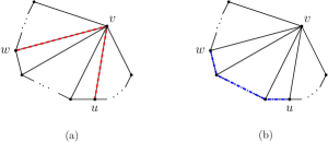
Figure 6: Two possible cases for the shortest path between $u$ and $w$: (a) it goes through vertex $v$ (shown in dashed red), or (b) it goes through the vertices of the $v$-chain between $u$ and $w$ (shown in dashed blue).

Lemma 10

After an $O(n)$–time preprocessing, we can report, for any three vertices $v$, $u$ and $w$, such that both $u$ and $w$ are vertices of $G[P_{v}]$, the beer distance $\mathsf{dist}_{B}(u,w)$ in $O(1)$ time. The corresponding shortest beer path $\mathsf{SP}_{B}(u,w)$ can be reported in $O(L)$ time, where $L$ is the number of vertices on the path.

Proof. Recall from Lemma 4 that we can compute $\mathsf{dist}_{B}(u,v)$ for every edge $(u,v)$ in $G$, and $\mathsf{dist}_{B}(v,v)$ for every vertex $v$ in $G$, in $O(n)$ time.

Let $\rho_{v}=(\mathsf{CW}(v)=u_{1},u_{2},\dots,u_{N}=\mathsf{CCW}(v))$. Let $A_{v}[~{}]$ be an array of size $N-1$. For $i=1,\ldots,N-1$, we set $A_{v}[i]=\mathsf{dist}_{B}(u_{i},u_{i+1})-\omega(u_{i},u_{i+1})$. Recall that by the generalized triangle inequality, $\omega(u_{i},u_{i+1})=\mathsf{dist}(u_{i},u_{i+1})$. Therefore, $A[i]$ holds the difference between the weights of the shortest path from $u_{i}$ to $u_{i+1}$ and the shortest beer path from $u_{i}$ to $u_{i+1}$. After preprocessing the array $A_{v}[~{}]$ in $O(N)$ time, we can conduct range minimum queries in $O(1)$ time. (Bender and Farach-Colton [2] show that these queries are equivalent to $\mathsf{LCA}$-queries in the Cartesian tree of the array.) Thus, for each $v$-chain of $N$ nodes, we spend $O(N)$ time processing the $v$-chain. Since every edge is in at most two chains, processing all $v$-chains takes $O(n)$ time and space.

Given two vertices $u$ and $w$ of $G[P_{v}]$, we determine the beer distance $\mathsf{dist}_{B}(u,w)$ as follows:

1. If $u=w$ then $\mathsf{dist}_{B}(u,w)$ has already been computed by Lemma 4.

2. If $u=v$ or $w=v$, then there is an edge from $v$ to the other vertex. Thus, $\mathsf{dist}_{B}(u,w)$ has already been computed by Lemma 4.

3. Otherwise, $u$, $w$ and $v$ are three distinct vertices. Assume without loss of generality that $w$ is clockwise from $u$ on the $v$-chain. We take the minimum of the following two cases:

   1. The shortest beer path from $u$ to $w$ that goes through $v$. Since a beer store must be visited before or after $v$, this beer path has a weight of $\min(\mathsf{dist}_{B}(u,v)+\omega(v,w),\omega(u,v)+\mathsf{dist}_{B}(v,w))$.

   2. The shortest beer path through the vertices of the $v$-chain. Note that this beer path will visit each vertex on the $v$-chain between $u$ and $w$, but may go off the $v$-chain to visit a beer store. On $\mathsf{SP}_{B}(u,w)$, there is one pair of vertices, $u_{i}$ and $u_{i+1}$, such that a beer path is taken between $u_{i}$ and $u_{i+1}$, and $u_{i}$ and $u_{i+1}$ are adjacent on the $v$-chain; refer to Figure 7. The shortest path is taken between all other pairs of adjacent vertices on the $v$-chain. From Lemma 7, we can compute $\mathsf{dist}(u,w,\rho_{v})$ in $O(1)$ time. The shortest beer path through the vertices of the $v$-chain has a weight of $\mathsf{dist}(u,w,\rho_{v})+A_{v}[i]$, where $A_{v}[i]$ is the additional distance needed to visit a beer store between $u_{i}$ and $u_{i+1}$. Let $u$ be the $j^{th}$ vertex on $\rho_{v}$ and let $w$ be the $k^{th}$ vertex in $\rho_{v}$. Then $A_{v}[i]$ is the minimum value in $A_{v}[j,\dots,k-1]$. We can determine $A_{v}[i]$ in constant time using a range minimum query.

Note that in case 1 and case 2, $\mathsf{SP}_{B}(u,w)$ can be constructed in $O(L)$ time by Lemma 4. For case 3 (a) let $p=(u,v,w)$ and for case 3 (b) let $p=\mathsf{SP}(u,w,\rho_{v})$. Let $u_{i}$, $u_{i+1}$ be the pair of adjacent vertices on $p$ between which a beer path was taken. Using Lemma 4 we can find $\mathsf{SP}_{B}(u_{i},u_{i+1})$ in $O(L)$ time. We obtain $\mathsf{SP}_{B}(u,w)$ by replacing the edge $(u_{i},u_{i+1})$ in $p$ with $\mathsf{SP}_{B}(u_{i},u_{i+1})$.   

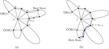
Figure 7: Both figures show a shortest beer path from $u$ to $w$ through the vertices on the $v$-chain. Thicker edges on the blue beer path are edges that are traversed twice; once in each direction.

4.1 Answering Shortest Beer Path Queries

Recall that, for any vertex $v$ of $G$, $P_{v}$ denotes the path in $D(G)$ formed by the faces of $G$ containing $v$. Moreover, $G[P_{v}]$ denotes the subgraph of $G$ induced by these faces.

Consider two query vertices $s$ and $t$ of $G$. Our goal is to compute the shortest beer path $\mathsf{SP}_{B}(s,t)$.

Let $F_{s}$ and $F_{t}$ be arbitrary faces containing $s$ and $t$, respectively. If $t$ is in $G[P_{s}]$ then, by Lemma 10, we can construct $\mathsf{SP}_{B}(s,t)$ in $O(L)$ time. For the remainder of this section, we assume that $t$ is not in $G[P_{s}]$. To find $\mathsf{SP}_{B}(s,t)$, we start by constructing a directed acyclic graph (DAG), $H$. In this DAG, vertices will be arranged in columns of constant size, and all edges go from left to right between vertices in adjacent columns. In $H$, each column will contain one vertex that is on $\mathsf{SP}_{B}(s,t)$. First we will construct $H$ and then we will show how we can use $H$ to construct $\mathsf{SP}_{B}(s,t)$. The entire construction is illustrated in Figure 8.

Observation 3

Any interior edge $(a,b)$ of $G$ splits $G$ into two subgraphs such that if $s$ is in one subgraph and $t$ is in the other, then any path in $G$ from $s$ to $t$ must visit at least one of $a$ and $b$.

Let $P$ be the unique path between $F_{s}$ and $F_{t}$ in $D(G)$. Consider moving along $P$ from $F_{s}$ to $F_{t}$. Let $F_{1}$ be the node on $P_{s}$ that is closest to $F_{t}$, and let $F^{\prime}_{1}$ be the successor of $F_{1}$ on $P$. Note that, by Lemmas 1 and 2, we can find $F_{1}$ and $F^{\prime}_{1}$ in $O(1)$ time. Let $e_{1}=(a_{1},b_{1})$ be the edge in $G$ shared by the faces $F_{1}$ and $F^{\prime}_{1}$. Since $\mathsf{SP}_{B}(s,t)$ must visit both of these faces, by Observation 3, at least one of $a_{1}$ or $b_{1}$ is on the shortest beer path.

We place $s$ in the first column of $H$ and $a_{1}$ and $b_{1}$ in the second column of $H$. We then add two directed edges from $s$ to $a_{1}$, one with weight $\mathsf{dist}(s,a_{1})$ and the other with weight $\mathsf{dist}_{B}(s,a_{1})$. Similarly, we add two directed edges from $s$ to $b_{1}$ with weights $\mathsf{dist}(s,b_{1})$ and $\mathsf{dist}_{B}(s,b_{1})$.

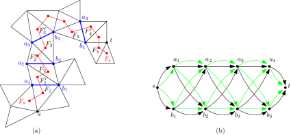
Figure 8: An outerplanar graph $G$ (a) and the DAG $H$ constructed for the shortest beer path query from $s$ to $t$ (b). The path $P$ from $F_{s}$ to $F_{t}$ is shown in red. Each edge $e_{i}=(a_{i},b_{i})$ such that $e_{i}$ is shared by $F_{i}$ and $F^{\prime}_{i}$ is shown in blue. The green edges of $H$ represent the beer edges.

When $i\geq 2$ we construct the $(i+1)^{th}$ column of $H$ in the following way. Let $e_{i-1}=(a_{i-1},b_{i-1})$ be the edge shared by the faces $F_{i-1}$ and $F^{\prime}_{i-1}$. The $i^{th}$ column of $H$ contains the vertices $a_{i-1}$ and $b_{i-1}$. Note that $F^{\prime}_{i-1}$ is in both $P_{b_{i-1}}$ and $P_{a_{i-1}}$. Using Lemma 2, we find the node $F_{i}^{b}$ on $P_{b_{i-1}}$ that is closest to $F_{t}$. If the vertex $a_{i-1}$ is not in $F_{i}^{b}$, then we let $F_{i}=F_{i}^{b}$. Otherwise, we let $F_{i}$ be the node on $P_{a_{i-1}}$ that is closest to $F_{t}$.

If $t$ is not a vertex of $F_{i}$, then let $F^{\prime}_{i}$ be the node that follows $F_{i}$ on $P$; we find $F^{\prime}_{i}$ using Lemma 1. Let $e_{i}=(a_{i},b_{i})$ be the edge of $G$ shared by the faces $F_{i}$ and $F^{\prime}_{i}$. In the $(i+1)^{th}$ column, we place $a_{i}$ and $b_{i}$. For each $u\in\{a_{i-1},b_{i-1}\}$ and each $v\in\{a_{i},b_{i}\}$ we add two directed edges $(u,v)$ to the DAG, one with weight $\mathsf{dist}(u,v)$ and the other with weight $\mathsf{dist}_{B}(u,v)$. If $F_{i}$ is in $P_{a_{i-1}}$, all these vertices are in $G[P_{a_{i-1}}]$; otherwise, $F_{i}$ is in $P_{b_{i-1}}$, and all these vertices are in $G[P_{b_{i-1}}]$. Thus, by Lemmas 8 and 10, we can find the distances and beer distances to assign to these edges in constant time.

If $t$ is in $F_{i}$, then in the $(i+1)^{th}$ column we only place the vertex $t$. In this case, for each $u\in\{a_{i-1},b_{i-1}\}$, we add two directed edges $(u,t)$ to the DAG with weights $\mathsf{dist}(u,t)$ and $\mathsf{dist}_{B}(u,t)$. At this point we are done constructing $H$.

We define a beer edge to be an edge of $H$ that was assigned a weight of a beer path during the construction of $H$. We find the beer distance from $s$ to $t$ in $G$ using the following dynamic programming approach in $H$.

Let $M$ denote the number of columns in $H$. For $i=3,\dots,M$ and for all $u$ in the $i^{th}$ column of $H$, compute

$$\mathsf{dist}_{B}(s,u)=\min\begin{cases}\mathsf{dist}_{B}(s,a_{i-2})+\mathsf{dist}(a_{i-2},u),\\ \mathsf{dist}(s,a_{i-2})+\mathsf{dist}_{B}(a_{i-2},u),\\ \mathsf{dist}_{B}(s,b_{i-2})+\mathsf{dist}(b_{i-2},u),\\ \mathsf{dist}(s,b_{i-2})+\mathsf{dist}_{B}(b_{i-2},u)\end{cases}$$

and

$$\mathsf{dist}(s,u)=\min\begin{cases}\mathsf{dist}(s,a_{i-2})+\mathsf{dist}(a_{i-2},u),\\ \mathsf{dist}(s,b_{i-2})+\mathsf{dist}(b_{i-2},u).\\ \end{cases}$$

The vertices $a_{i-2}$ and $b_{i-2}$ occur in the $(i-1)^{th}$ column. Thus, $\mathsf{dist}_{B}(s,a_{i-2})$, $\mathsf{dist}_{B}(s,b_{i-2})$, $\mathsf{dist}(s,a_{i-2})$, and $\mathsf{dist}(s,b_{i-2})$ will be computed before computing the values for the $i^{th}$ column. We get $\mathsf{dist}(a_{i-2},u)$, $\mathsf{dist}_{B}(a_{i-2},u)$, $\mathsf{dist}(b_{i-2},u)$ and $\mathsf{dist}_{B}(b_{i-2},u)$ from the weights of the DAG-edges between the $(i-1)^{th}$ and $i^{th}$ columns of $H$.

By keeping track of which expression produced $\mathsf{dist}_{B}(s,u)$ and $\mathsf{dist}(s,u)$, we can backwards reconstruct the shortest beer path in the DAG. Knowing the shortest beer path in the DAG enables us to construct the corresponding beer path in $G$ as follows.

1. Define $P_{st}$ to be an empty path.

2. For each edge $(w,v)$ of the shortest beer path in the DAG.

   1. If $(w,v)$ was a beer edge, let $P_{wv}=\mathsf{SP}_{B}(w,v)$, which can be constructed in time proportional to its number of vertices via Lemma 10.

   2. Otherwise, let $P_{wv}=\mathsf{SP}(w,v)$ which can be constructed in time proportional to its number of vertices as seen in Lemma 9.

   Let $P_{st}=P_{st}\cup P_{wv}$.

3. Return $P_{st}$, which is equal to $\mathsf{SP}_{B}(w,v)$.

Let $L$ denote the number of vertices on $\mathsf{SP}_{B}(s,t)$. In order for the above query algorithm to take $O(L)$ time, the size of the DAG must be $O(L)$. The following three lemmas will show this to be true.

Lemma 11

For $2\leq i<M-1$, $F_{i}$ contains either $a_{i-1}$ or $b_{i-1}$, but not both.

Proof. Recall that we defined $F_{i}^{b}$ to be the last node on $P$ that is also on $P_{b_{i-1}}$. We similarly define $F_{i}^{a}$ to be the last node on $P$ that is also on $P_{a_{i-1}}$. From the way we choose $F_{i}$, $F_{i}$ is either $F_{i}^{b}$ or $F_{i}^{a}$. We only choose $F_{i}=F_{i}^{b}$ after having checked that $a_{i-1}$ is not in $F_{i}^{b}$; thus in this case we can be sure that $F_{i}$ only contains $b_{i-1}$.

Assume for the purpose of contradiction that we choose $F_{i}=F_{i}^{a}$ and $b_{i-1}$ is also in $F_{i}$. Let the third vertex of $F_{i}$ be $c$. Let the face on $P$ immediately following $F_{i}$ be $F_{i}^{\prime}$. The edge shared by $F_{i}$ and $F^{\prime}_{i}$ is either $(b_{i-1},c)$ or $(a_{i-1},c)$. If $(b_{i-1},c)$ is the shared edge, then $F_{i}^{\prime}$ is a face closer to $F_{t}$ that contains $b_{i-1}$ and not $a_{i-1}$, so we would have chosen $F_{i}=F_{i}^{b}$, which is a contradiction. Otherwise, $(a_{i-1},c)$ is the edge shared by $F_{i}$ and $F_{i}^{\prime}$, which implies that there is a face containing $a_{i-1}$ closer to $F_{t}$ in $P$ than $F_{i}^{a}$, which contradicts the definition of $F_{i}^{a}$.   

Lemma 12

Every vertex of $G$ appears in at most one column of $H$.

Proof. Since $(a_{1},b_{1})$ is an edge shared by both the last face of $P$ containing $s$ and the first face of $P$ that does not contain $s$ it is not possible for either of these vertices to be the vertex $s$. Thus, $s$ will only be represented by the vertex in the first column of $H$. By stopping the construction of $H$ as soon as we add a vertex representing $t$, we ensure that $H$ only contains one vertex corresponding to the vertex $t$ in $G$.

For $2\leq i\leq M-2$, consider the vertex $a_{i-1}$ in $G$ represented by a vertex in the $i^{th}$ column of $H$. If $F_{i}=F_{i}^{a}$ then by definition of $F_{i}^{a}$, $F^{\prime}_{i}$ does not contain $a_{i-1}$. Since $(a_{i},b_{i})$ is an edge of $F^{\prime}_{i}$, $a_{i}\neq a_{i-1}$ and $b_{i}\neq a_{i-1}$. Because the face $F^{\prime}_{i}$ is closer to $F_{t}$ than $F_{i}^{a}$, $a_{i-1}$ is not a vertex on any of the faces on the path from $F^{\prime}_{i}$ to $F_{t}$. Thus, subsequent columns of $H$ will not contain vertices representing the vertex $a_{i-1}$ in $G$.

If $F_{i}=F_{i}^{b}$ then by Lemma 11, $a_{i-1}$ is not in $F_{i}$ and since $(a_{i},b_{i})$ is an edge of $F_{i}$, $a_{i}\neq a_{i-1}$ and $b_{i}\neq a_{i-1}$. Because $F_{i}$ is a face on $P$ closer to $F_{t}$ than $F_{i-1}$ (a face that contains $a_{i-1}$) it follows from Observation 2 that none of the faces on $P$ from $F_{i-1}$ to $F_{t}$ will have the vertex $a_{i-1}$ on their face and, thus, $a_{i-1}$ will not be represented by vertices in subsequent columns of $H$.

By switching the roles of $a_{i-1}$ with $b_{i-1}$ in the above reasoning we can see that this also holds for $b_{i-1}$.   

Lemma 13

The number of vertices and edges of $H$ is $O(L)$.

Proof. By Observation 3 and Lemma 12, the number of columns of $H$ is at most $L$. Since each column has at most two vertices, each of which having at most four outgoing edges, the total number of vertices and edges of $H$ is $O(L)$.   

Observe that the total preprocessing time is $O(n)$. For two query vertices $s$ and $t$, the DAG, $H$, can be constructed in $O(L)$ time. Finally, the dynamic programming algorithm on $H$ takes $O(L)$ time. Thus, we have proved Theorem 2 for maximal outerplanar graphs that satisfy the generalized triangle inequality.

5 Proof of Lemma 4

Let $G$ be a maximal outerplanar beer graph with $n$ vertices that satisfies the generalized triangle inequality. We will first show how to compute $\mathsf{dist}_{B}(u,u)$ for each vertex $u$ of $G$, and $\mathsf{dist}_{B}(u,v)$ for each edge $(u,v)$ of $G$. Consider again the dual $D(G)$ of $G$. We choose an arbitrary face of $G$ and make it the root of $D(G)$.

Let $(u,v)$ be any edge of $G$. This edge divides $G$ into two outerplanar subgraphs, both of which contain $(u,v)$ as an edge. Let $G_{uv}^{R}$ be the subgraph that contains the face represented by the root of $D(G)$, and let $G_{uv}^{\neg R}$ denote the other subgraph. Note that if $(u,v)$ is an external edge, then $G_{uv}^{R}=G$ and $G_{uv}^{\neg R}$ consists of the single edge $(u,v)$.

By the generalized triangle inequality, the shortest beer path between $u$ and $v$ is completely in $G_{uv}^{R}$ or completely in $G_{uv}^{\neg R}$. The same is true for the shortest beer path from $u$ to itself. This implies:

Observation 4

For each edge $(u,v)$ of $G$,

1. $\mathsf{dist}_{B}(u,v)=\min\left(\mathsf{dist}_{B}(u,v,G_{uv}^{R}),\mathsf{dist}_{B}(u,v,G_{uv}^{\neg R})\right)$,

2. $\mathsf{dist}_{B}(u,u)=\min\left(\mathsf{dist}_{B}(u,u,G_{uv}^{R}),\mathsf{dist}_{B}(u,u,G_{uv}^{\neg R})\right)$,

3. $\mathsf{dist}_{B}(v,v)=\min\left(\mathsf{dist}_{B}(v,l,G_{uv}^{R}),\mathsf{dist}_{B}(v,v,G_{uv}^{\neg R})\right)$,

Thus, it suffices to first compute $\mathsf{dist}_{B}(u,v,G_{uv}^{\neg R})$, $\mathsf{dist}_{B}(u,u,G_{uv}^{\neg R})$, and $\mathsf{dist}_{B}(v,v,G_{uv}^{\neg R})$ for all edges $(u,v)$, and then compute $\mathsf{dist}_{B}(u,v,G_{uv}^{R})$, $\mathsf{dist}_{B}(u,u,G_{uv}^{R})$, and $\mathsf{dist}_{B}(v,v,G_{uv}^{R})$, again for all edges $(u,v)$.

5.1 Recurrences for $\mathsf{dist}_{B}(u,v,G_{uv}^{\neg R})$, $\mathsf{dist}_{B}(u,u,G_{uv}^{\neg R})$, and $\mathsf{dist}_{B}(v,v,G_{uv}^{\neg R})$

Let $(u,v)$ be an edge of $G$. Item 1. below presents the base cases, whereas item 2. gives the recurrences.

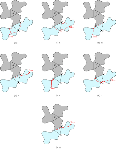
Figure 9: Illustrating the post-order traversal for all cases in item 2.

1. Assume that $(u,v)$ is an external edge of $G$.

   1. If both $u$ and $v$ are beer stores, then $\mathsf{dist}_{B}(u,v,G_{uv}^{\neg R})=\omega(u,v)$, $\mathsf{dist}_{B}(u,u,G_{uv}^{\neg R})=0$, and $\mathsf{dist}_{B}(v,v,G_{uv}^{\neg R})=0$.

   2. If exactly one of $u$ and $v$, say $u$, is a beer store, then $\mathsf{dist}_{B}(u,v,G_{uv}^{\neg R})=\omega(u,v)$, $\mathsf{dist}_{B}(u,u,G_{uv}^{\neg R})=0$, and $\mathsf{dist}_{B}(v,v,G_{uv}^{\neg R})=2\cdot\omega(u,v)$.

   3. If neither $u$ nor $v$ is a beer store, then $\mathsf{dist}_{B}(u,v,G_{uv}^{\neg R})=\infty$, $\mathsf{dist}_{B}(u,u,G_{uv}^{\neg R})=\infty$, and $\mathsf{dist}_{B}(v,v,G_{uv}^{\neg R})=\infty$.

2. Assume that $(u,v)$ is an internal edge of $G$. Let $w$ be the third vertex of the face of $G_{uv}^{\neg R}$ that contains $(u,v)$ as an edge. All possible cases are illustrated in Figure 9.

   1. The value of $\mathsf{dist}_{B}(u,v,G_{uv}^{\neg R})$ is the minimum of

      1. $\mathsf{dist}_{B}(u,w,G_{uw}^{\neg R})+\omega(w,v)$,

      2. $\omega(u,w)+\mathsf{dist}_{B}(w,v,G_{vw}^{\neg R})$,

      3. $\mathsf{dist}_{B}(u,u,G_{uw}^{\neg R})+\omega(u,v)$,

      4. $\omega(u,v)+\mathsf{dist}_{B}(v,v,G_{vw}^{\neg R})$.

   2. The value of $\mathsf{dist}_{B}(u,u,G_{uv}^{\neg R})$ is the minimum of

      1. $\mathsf{dist}_{B}(u,u,G_{uw}^{\neg R})$,

      2. $2\cdot\omega(u,w)+\mathsf{dist}_{B}(w,w,G_{vw}^{\neg R})$,

      3. $2\cdot\omega(u,v)+\mathsf{dist}_{B}(v,v,G_{vw}^{\neg R})$.

      The value of $\mathsf{dist}_{B}(v,v,G_{uv}^{\neg R})$ is obtained by swapping $u$ and $v$ in i., ii., and iii.

These recurrences express $\mathsf{dist}_{B}(u,v,G_{uv}^{\neg R})$, $\mathsf{dist}_{B}(u,u,G_{uv}^{\neg R})$, and $\mathsf{dist}_{B}(v,v,G_{uv}^{\neg R})$ in terms of values that are “further down” in the tree $D(G)$. Therefore, by performing a post-order traversal of $D(G)$, we obtain all these values, for all edges $(u,v)$ of $G$, in $O(n)$ total time.

5.2 Recurrences for $\mathsf{dist}_{B}(u,v,G_{uv}^{R})$, $\mathsf{dist}_{B}(u,u,G_{uv}^{R})$, and $\mathsf{dist}_{B}(v,v,G_{uv}^{R})$

Let $(u,v)$ be an edge of $G$. Item 1. below presents the base cases, whereas item 2. gives the recurrences.

1. Assume that $(u,v)$ is an edge of the face representing the root of $D(G)$. Let $w$ be the third vertex of this face.

   1. The value of $\mathsf{dist}_{B}(u,v,G_{uv}^{R})$ is the minimum of

      1. $\mathsf{dist}_{B}(u,u,G_{uw}^{\neg R})+\omega(u,v)$,

      2. $\mathsf{dist}_{B}(u,w,G_{uw}^{\neg R})+\omega(w,v)$,

      3. $\omega(u,v)+\mathsf{dist}_{B}(v,v,G_{vw}^{\neg R})$,

      4. $\omega(u,w)+\mathsf{dist}_{B}(w,v,G_{vw}^{\neg R})$.

   2. The value of $\mathsf{dist}_{B}(u,u,G_{uv}^{R})$ is the minimum of

      1. $\mathsf{dist}_{B}(u,u,G_{uw}^{\neg R})$,

      2. $2\cdot\omega(u,w)+\mathsf{dist}_{B}(w,w,G_{vw}^{\neg R})$,

      3. $2\cdot\omega(u,v)+\mathsf{dist}_{B}(v,v,G_{vw}^{\neg R})$.

      The value of $\mathsf{dist}_{B}(v,v,G_{uv}^{\neg R})$ is obtained by swapping $u$ and $v$ in i., ii., and iii.

2. Assume that $(u,v)$ is not an edge of the face represented by the root of $D(G)$. Let $w$ be the third vertex of the face of $G_{uv}^{R}$ that contains $(u,v)$ as an edge. We may assume without loss of generality that $(v,w)$ is an edge of the face represented by the parent of the face representing $(u,v,w)$. All possible cases are illustrated in Figure 10.

   

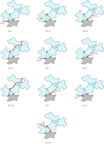
   Figure 10: Illustrating the pre-order traversal for all cases in item 2.

   1. The value of $\mathsf{dist}_{B}(u,v,G_{uv}^{R})$ is the minimum of

      1. $\mathsf{dist}_{B}(u,u,G_{uw}^{\neg R})+\omega(u,v)$,

      2. $\mathsf{dist}_{B}(u,w,G_{uw}^{\neg R})+\omega(w,v)$,

      3. $\omega(u,v)+\mathsf{dist}_{B}(v,v,G_{vw}^{R})$,

      4. $\omega(u,w)+\mathsf{dist}_{B}(w,v,G_{vw}^{R})$.

   2. The value of $\mathsf{dist}_{B}(u,u,G_{uv}^{R})$ is the minimum of

      1. $\mathsf{dist}_{B}(u,u,G_{uw}^{\neg R})$,

      2. $2\cdot\omega(u,v)+\mathsf{dist}_{B}(v,v,G_{vw}^{R})$,

      3. $2\cdot\omega(u,w)+\mathsf{dist}_{B}(w,w,G_{vw}^{R})$.

   3. The value of $\mathsf{dist}_{B}(v,v,G_{uv}^{R})$ is the minimum of

      1. $\mathsf{dist}_{B}(v,v,G_{vw}^{R})$,

      2. $2\cdot\omega(v,u)+\mathsf{dist}_{B}(u,u,G_{uw}^{R})$,

      3. $2\cdot\omega(v,w)+\mathsf{dist}_{B}(w,w,G_{uw}^{R})$.

These recurrences express $\mathsf{dist}_{B}(u,v,G_{uv}^{R})$, $\mathsf{dist}_{B}(u,u,G_{uv}^{R})$, and $\mathsf{dist}_{B}(v,v,G_{uv}^{R})$ in terms of values that are “higher up” in the tree $D(G)$ and values that involve graphs with a superscript “$\neg R$”. These latter values have been computed already. Thus, by performing a pre-order traversal of $D(G)$, we obtain all values $\mathsf{dist}_{B}(u,v,G_{uv}^{R})$, $\mathsf{dist}_{B}(u,u,G_{uv}^{R})$, and $\mathsf{dist}_{B}(v,v,G_{uv}^{R})$, for all edges $(u,v)$ of $G$, in $O(n)$ total time. This completes the proof of the first claim in Lemma 4.

Consider $\mathsf{dist}(u,v)$ where $u=v$ or $(u,v)$ is an edge of $G$. If $u$ or $v$ is a beer store, then store $nil$ with $\mathsf{dist}(u,v)$.

The values $\mathsf{dist}(u,v,G_{uv}^{R})$ and $\mathsf{dist}(u,v,G_{uv}^{\neg R})$ are computed as the minimum of a set of path weights from $u$ to $v$ through a vertex $x$ such that $x$ is adjacent to both $u$ and $v$ or $x$ is equal to one of these vertices and adjacent to the other. Either the subpath from $u$ to $x$ is a beer path or the subpath from $x$ to $v$ is a beer path. Whenever we take the minimum of a set of path weights in the above computation, we store with that distance the vertex $x$ and a bit to indicate which subpath is the beer path. When $u=v$ we can arbitrarily choose which subpath is the beer path. After taking the minimum of $\mathsf{dist}(u,v,G_{uv}^{R})$ and $\mathsf{dist}(u,v,G_{uv}^{\neg R})$, we are left with a vertex, $x$, on the shortest beer path from $u$ to $v$ and the bit indicating which subpath is a beer path.

We recursively compute $\mathsf{SP}_{B}(u,v)$ where either $(u,v)$ is an edge of $G$ or $u=v$ as follows.

1. If $nil$ is stored with $\mathsf{dist}_{B}(u,v)$ and $u=v$, $\mathsf{SP}_{B}(u,v)=(u)$.

2. If $nil$ is stored with $\mathsf{dist}_{B}(u,v)$ and $(u,v)$ is an edge then $\mathsf{SP}_{B}(u,v)=(u,v)$.

3. If a vertex $x$ is stored with $(u,v)$ and the subpath from $u$ to $x$ is a beer path then recursively compute $\mathsf{dist}_{B}(u,x)$. $\mathsf{SP}_{B}(u,v)=\mathsf{SP}_{B}(u,x)\cup(v)$.

4. Otherwise $x$ is stored with $(u,v)$ and the subpath from $x$ to $v$ is a beer path. Recursively compute $\mathsf{dist}_{B}(x,v)$. $\mathsf{SP}_{B}(u,v)=(u)\cup\mathsf{SP}_{B}(x,v)$.

Note that a constant amount of work is done at each level of the recurrence excluding the time spent in recursive calls. In each recursive call, except potentially the last call, we get one new vertex on the shortest beer path. Thus, constructing the whole path requires a total of $O(L)$ time.

6 Extension to Arbitrary Outerplanar Graphs

6.1 Maximal Outerplanar

Let $G$ be an outerplanar beer graph with $n$ vertices. Assume that the outer face of $G$ is not a Hamiltonian cycle. We traverse $G$ along the outer face in a clockwise manner, and mark each vertex when we encounter it for the first time. Each time we visit a marked vertex $v$, we take note of $v$’s current counterclockwise neighbor, $\mathsf{CCW}(v)$. Then we continue from $v$ to the next clockwise vertex on the outer face and add an edge from this vertex to $\mathsf{CCW}(v)$. We continue this process until we have returned to the vertex we started from and all vertices have been marked.

At this moment, the outer face is a Hamiltonian cycle. For every interior face that is not a triangle, we pick a vertex $u$ on that face and add edges connecting $u$ with all vertices of the face that are not already adjacent to $u$.

The resulting graph is a maximal outerplanar graph. Each edge that has been added is given a weight of infinity. Observe that each shortest (beer) path in the resulting graph corresponds to a shortest (beer) path in the original graph, and vice versa.

6.2 Generalized Triangle Inequality

Let $G$ be a maximal outerplanar graph with an edge weight function $\omega$. In order to convert $G$ to a graph that satisfies the generalized triangle inequality, we need to compute $\mathsf{dist}(u,v)$ for every edge $(u,v)$ in $G$, and we need to be able to construct $\mathsf{SP}(u,v)$ for each edge $(u,v)$.

Let $D(G)$ be the dual of $G$ rooted at an arbitrary interior face of $G$. For each edge $(u,v)$, we initialize $\delta(u,v)=\omega(u,v)$. (At the end, $\delta(u,v)$ will be equal to $\mathsf{dist}(u,v)$.) For each edge $(u,v)$, we also maintain a parent vertex, $p(u,v)$, initialized to $nil$.

We first conduct a post-order traversal of $D(G)$, processing each associated face in $G$. Then we conduct a pre-order traversal of $D(G)$, again processing each associated face in $G$. Let $F$ be a face of $G$. We process $F$ as follows. Let $(u,v)$ be the edge of $F$ that is shared with the predecessor face $F^{\prime}$ in the traversal, and let $w$ be the third vertex of $F^{\prime}$. If $\delta(u,v)>\delta(u,w)+\delta(w,v)$, we set $\delta(u,v)=\delta(u,w)+\delta(w,v)$ and $p(u,v)=w$.

After these traversals, $\delta(u,v)=\mathsf{dist}(u,v)$ for every edge $(u,v)$ in $G$. If $p(u,v)=nil$, then $\mathsf{SP}(u,v)=(u,v)$; otherwise, $\mathsf{SP}(u,v)$ is the concatenation of $\mathsf{SP}(u,p(u,v))$ and $\mathsf{SP}(p(u,v),v)$, both of which can be computed recursively.

7 Single Source Shortest Beer Path

In this section we will describe how to compute the single source shortest beer path from a source vertex $s$ on a maximal outerplanar graph $G$ that satisfies the generalized triangle inequality. In order to do this we first precompute (i) $\mathsf{dist}_{B}(u,v)$ for every edge $(u,v)$ and $\mathsf{dist}_{B}(u,u)$ for every vertex $u$ and (ii) $\mathsf{dist}(s,v)$ for every vertex $v$. By Lemma 4, we can compute (i) in $O(n)$ time and in [7], Maheshwari and Zeh present a single source shortest path algorithm for undirected outerplanar graphs which gives us (ii) in $O(n)$ time.

Let $D(G)$ be the dual of $G$ and let $F_{s}$ be an arbitrary interior face of $G$ containing $s$. Root $D(G)$ at the node $F_{s}$ and then conduct a pre-order traversal of $D(G)$. Let $F$ be the current node of $D(G)$ being processed during this traversal.

1. If $F=F_{s}$, let $u$ and $v$ be the vertices of $F_{s}$ that are not $s$. Since $(s,u)$ and $(s,v)$ are both edges of $G$, $\mathsf{dist}_{B}(s,s)$, $\mathsf{dist}_{B}(s,u)$ and $\mathsf{dist}_{B}(s,v)$ were precomputed in (i).

2. If $F\neq F_{s}$, let $a$ and $b$ be the vertices of $F$ shared with the face $F^{\prime}$, where $F^{\prime}$ is the parent of $F$ in $D(G)$. This implies that by this step we have already computed $\mathsf{dist}_{B}(s,a)$ and $\mathsf{dist}_{B}(s,b)$. Let $c$ be the third vertex of $F$. The value of $\mathsf{dist}_{B}(s,c)$ is the minimum of:

   1. $\mathsf{dist}(s,a)+\mathsf{dist}_{B}(a,c)$,

   2. $\mathsf{dist}_{B}(s,a)+\omega(a,c)$,

   3. $\mathsf{dist}(s,b)+\mathsf{dist}_{B}(b,c)$,

   4. $\mathsf{dist}_{B}(s,b)+\omega(b,c)$.

   Since $(a,c)$ and $(b,c)$ are edges of $G$ we precomputed $\mathsf{dist}_{B}(a,c)$ and $\mathsf{dist}_{B}(b,c)$ in (i). Lastly, we computed $\mathsf{dist}(s,a)$ and $\mathsf{dist}(s,b)$ in (ii) so each of the values listed above can be computed in constant time.

The correctness of this algorithm follows from Observation 3 and the generalized triangle inequality. Since we do a constant amount of work at each face in the traversal of $D(G)$ and the number of interior faces of a maximal outerplanar graph is $n-2$, this algorithm takes $O(n)$ time.

Let $L$ the the number of vertices on the shortest beer path from $s$ to $v$. If $\mathsf{dist}_{B}(s,v)$ was found in step 1, then by Lemma 4, $\mathsf{SP}_{B}(s,v)$ can be constructed in $O(L)$ time. If this is not the case, then $v=c$ in some iteration of step 2. At this step we store a vertex $p(v)$ such that $p(v)=a$ if (a) or (b) was the minimum of step 2 and $p(v)=b$ otherwise. We also store a bit to indicate if the subpath from $s$ to $p(v)$ is the shortest path (as in cases (a) and (c)) or the shortest beer path (as in cases (b) and (d)). If the subpath from $s$ to $p(v)$ is the shortest path, we use the method described in [7] to find $\mathsf{SP}(s,p(v))$ and use Lemma 4 to find $\mathsf{SP}_{B}(p(v),v)$ and then concatenate $\mathsf{SP}(s,p(v))$ and $\mathsf{SP}_{B}(p(v),v)$ to get $\mathsf{SP}_{B}(s,v)$. Both $\mathsf{SP}(s,p(v))$ and $\mathsf{SP}_{B}(p(v),v)$ are found in time proportional to the number of vertices on their paths, so this takes $O(L)$ time. If the subpath from $s$ to $p(v)$ is the shortest beer path, then we recursively find $\mathsf{SP}_{B}(s,p(v))$ and concatenate it with the edge $(p(v),v)$ (which is $\mathsf{SP}(p(v),v)$ by the generalized triangle inequality). Each iteration of the recursive step takes time proportional to the number of new vertices of the path found in that step. Thus, we find $\mathsf{SP}_{B}(s,v)$ in a total of $O(L)$ time.

References

- [1] N. Alon and B. Schieber. Optimal preprocessing for answering on-line product queries. Technical Report 71/87, Tel-Aviv University, 1987.
- [2] M. A. Bender and M. Farach-Colton. The LCA problem revisited. In Proceedings of the 4th Latin American Symposium on Theoretical Informatics, volume 1776 of Lecture Notes in Computer Science, pages 88–94, Berlin, 2000. Springer-Verlag.
- [3] T. M. Chan, M. He, J. I. Munro, and G. Zhou. Succinct indices for path minimum, with applications. Algorithmica, 78(2):453–491, 2017.
- [4] B. Chazelle. Computing on a free tree via complexity-preserving mappings. Algorithmica, 2:337–361, 1987.
- [5] H. Djidjev, G. E. Pantziou, and C. D. Zaroliagis. Computing shortest paths and distances in planar graphs. In Automata, Languages and Programming, 18th International Colloquium, ICALP91, volume 510 of Lecture Notes in Computer Science, pages 327–338. Springer, 1991.
- [6] D. Harel and R. E. Tarjan. Fast algorithms for finding nearest common ancestors. SIAM J. Comput., 13(2):338–355, 1984.
- [7] A. Maheshwari and N. Zeh. I/o-optimal algorithms for outerplanar graphs. Journal of Graph Algorithms and Applications, 8(1):47–87, 2004.
- [8] S. Pettie. An inverse-Ackermann type lower bound for online minimum spanning tree verification. Combinatorica, 26(2):207–230, 2006.
- [9] M. Thorup. Parallel shortcutting of rooted trees. Journal of Algorithms, 32:139–159, 1997.