DCPT/21/86, DESY-21-174, IPPP/21/43, MCNET-21-14, SAGEX-21-33 HEJ 2.1: High-energy Resummation with Vector Bosons and Next-to-Leading Logarithms

Abstract

We present version 2.1 of the High Energy Jets (HEJ) event generator for hadron colliders. HEJ is a Monte Carlo generator for processes at high energies with multiple well-separated jets in the final state. To achieve accurate predictions, conventional fixed-order perturbative QCD is supplemented with an all-order resummation of large high-energy logarithms. The new version 2.1 now supports processes with final-state leptons originating from a charged or neutral vector boson together with multiple jets, in addition to processes available in earlier versions. Furthermore, the all-order resummation is extended to include an additional gauge-invariant class of subdominant logarithmic corrections. HEJ 2.1 can be obtained from https://hej.hepforge.org.

1 Introduction

High Energy Jets (HEJ) is a Monte Carlo event generator for processes involving two or more jets. It implements the eponymous formalism for the all-order summation of high-energy logarithms in $\tfrac{\hat{s}}{p_{t}^{2}}$ developed in [1, 2, 3]. This summation is necessary to obtain a good description of events with large invariant masses or large rapidity separations between the outgoing particles. Extensive reviews of the formalism can be found in [4, 5].

HEJ has been validated against data in numerous studies on pure multijet production [6, 7, 8, 9], production of a leptonically decaying W boson together with two or more jets [10, 11, 12], and the production of multiple jets together with two charged leptons, created from an intermediate photon or Z boson [13]. A further particularly interesting channel is the gluon-fusion production of a Higgs boson together with two or more jets. It constitutes the dominant background in measurements of Higgs boson production in weak boson fusion (VBF), and the application of typical VBF cuts projects out a region of phase space where the summation of high-energy logarithms yields significant corrections [14]. For this process, as well as for pure multijet production, the original leading-logarithmic (LL) summation was supplemented with a numerically important gauge-invariant subset of the next-to-leading-logarithmic (NLL) corrections to achieve a better description away from the asymptotic high-energy limit [4].

A complete redesign allowed to extend the matching between resummation and fixed-order predictions to the highest multiplicities [15], taking into account at the same time quark mass corrections in the gluon-fusion production of a Higgs boson together with jets [16]. This revised matching procedure, initially implemented for pure multijet and Higgs boson plus jets production, is the foundation of HEJ 2 [17].

Here, we present HEJ 2.1. This new version elevates the fixed-order matching for the aforementioned processes involving an intermediate W or Z boson or photon to the superior HEJ 2 procedure. Furthermore, it includes a new subset of NLL corrections for pure multijet production and the production of a W boson together with jets. With these additions, HEJ 2.1 supersedes all earlier HEJ versions. We briefly describe the addition of the processes involving intermediate vector bosons and the new NLL corrections associated with the emission of additional quark-antiquark pairs in section 2. In section 3, we give an explicit example demonstrating how HEJ 2.1 can be used to supplement leading-order descriptions of the production of two leptons with jets with high-energy resummation. We conclude in section 4.

2 Improvements over previous versions

The most significant improvements over previous versions of HEJ are the addition of high-energy resummation for the production of two leptons together with two or more jets and the inclusion of NLL corrections involving the production of an additional quark-antiquark pair. In the following, we briefly summarise how these new processes are described in the High Energy Jets formalism. A more detailed description of both the underlying formalism and the improvements discussed here is given in [5]. The changes are summarised in table 1.

Process	LL	NLL unordered gluon	NLL quark-antiquark
$\geq$2 jets	HEJ 2.0	HEJ 2.0	HEJ 2.1
H + $\geq$2 jets	HEJ 2.0	HEJ 2.0	—
W + $\geq$2 jets	HEJ 2.1	HEJ 2.1	HEJ 2.1
Z/$\gamma$ + $\geq$2 jets	HEJ 2.1	HEJ 2.1	—

Table 1: Implemented processes and higher-order logarithmic corrections in HEJ

2.1 Leading-logarithmic resummation in HEJ 2

In HEJ 2, fixed-order predictions are supplemented with high-energy resummation in the following way. First, a number of leading-order events are generated. Then, for each event, it is determined whether the corresponding matrix element contributes at a logarithmic accuracy that is included in the current state-of-the art HEJ resummation. While HEJ currently includes partial NLL resummation, we restrict the following discussion to LL resummation for the sake of clarity.

To identify event configurations contributing at LL accuracy, we order incoming and outgoing particles according to rapidity, see figure 1. We then draw a leading-order auxiliary diagram with as many $t$-channel gluons as possible. It should be stressed that this diagram only serves to determine the logarithmic order and is never used to compute the actual matrix element. A configuration contributes at LL accuracy iff the number of $t$-channel gluons is maximal, i.e. if no other rapidity ordering of an equivalent set of final-state particles allows a diagram with a larger number of $t$-channel gluon exchanges. By “equivalent” we mean that we do not distinguish between parton flavours, such that all final states shown in figure 1 are treated on the same footing.

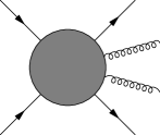
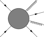
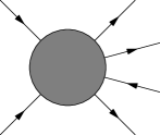
Figure 1: Identification of configurations with leading-logarithmic contributions. The leftmost configuration allows the maximum of three $t$-channel gluon exchanges and therefore contributes at LL accuracy. The remaining configurations permit at most two $t$-channel gluons. They are suppressed in the high-energy limit.

If the matrix element of the currently considered event contributes at a logarithmic order that is covered by the resummation, we replace the original event with a number of newly generated events. These new events add further gluon emissions, while preserving the rapidities of the original jets and non-parton particles. Details of the procedure are given in [15]. In order to obtain an all-order resummed prediction, while at the same time retaining leading-order accuracy, the newly generated events are reweighted by a factor

$$w_{\text{res}}=\frac{\overline{|{\cal M}^{\text{{\tt HEJ}}}|}^{2}}{\overline{|{\cal M}^{\text{{\tt HEJ}}}_{\text{LO}}|}^{2}},$$ (1)

where ${\cal M}^{\text{{\tt HEJ}}}$ is the all-order resummed matrix element in the high-energy limit and ${\cal M}^{\text{{\tt HEJ}}}_{\text{LO}}$ its leading-order truncation. The bar denotes the sum (average) over outgoing (incoming) helicities and colours.

The HEJ matrix elements are the only process-specific ingredient in the resummation procedure. In the following, we recall their general structure and give results for the new processes included in HEJ 2.1.

2.2 Leading-logarithmic matrix elements

We are interested in the LL HEJ matrix elements for processes $f_{a}f_{b}\to Xf_{a^{\prime}}\cdot ng\cdot f_{b^{\prime}}$, where $X$ denotes any number of additional colourless outgoing particles. With the exception of $X$, particles are ordered according to rapidity. $f_{a}$ is therefore the incoming parton in the backward direction, with flavour $a$, and $f_{b}$ the parton in the forward direction. The most backward outgoing parton is $f_{a^{\prime}}$ with rapidity $y_{1}$, followed by $n$ gluons with rapidities $y_{2}<\dots<y_{n+1}$ and the most forward outgoing parton $f_{b^{\prime}}$ with rapidity $y_{n+2}$.

In the absence of $X$, the outgoing flavours match the incoming ones, i.e. $a^{\prime}=a,b^{\prime}=b$. This is still the case if a charged lepton-antilepton pair $X=l\bar{l}$ is produced. However, for this process we require a virtual photon or Z boson, which implies that at least one of $f_{a}$ and $f_{b}$ has to be a quark or antiquark. When producing a pair of charged lepton and a neutrino, $X=l\bar{\nu}_{l}$ or $X=\bar{l}\nu_{l}$, a quark or antiquark couples to a virtual W boson. This means that the respective flavour is changed, so that either $a^{\prime}\neq a$ or $b^{\prime}\neq b$.

2.2.1 Matrix element without interference

The square of the LL HEJ matrix element in the absence of interference has the following structure, illustrated also in figure 2:

$$\begin{split}\overline{|{\cal M}^{\text{{\tt HEJ}}}_{f_{a}f_{b}\to Xf_{a^{\prime}}\cdot ng\cdot f_{b^{\prime}}}|}={}&{\color[rgb]{0,0,1}{\cal B}_{f_{a},f_{b},X}(p_{a},p_{b},p_{1},p_{n+2},\{p\}_{X})}\\ &\cdot\prod_{i=1}^{n}{\color[rgb]{.5,.5,.5}(p_{a},p_{b},p_{1},p_{n+2},q_{i},q_{i+1})}\\ &\cdot\prod_{i=1}^{n+1}{\color[rgb]{1,0,0}{\cal W}(q_{j},y_{j},y_{j+1})}\end{split}$$ (2)

$p_{a}$ and $p_{b}$ are the momenta of $f_{a}$ and $f_{b}$, $p_{i}$ with $1\leq i\leq n+2$ the outgoing momenta ordered by ascending rapidity, and $q_{j}$ the $t$-channel momenta related by $q_{j}=q_{j-1}-p_{j}$. The first $t$-channel momentum $q_{1}$ is process-dependent; if there are no additional particles $X$ it is given by $q_{1}=p_{a}-p_{1}$. $\{p\}_{X}$ represents the local momenta associated with the production of $X$.

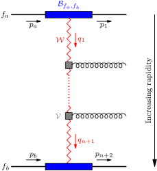
Figure 2: Structure of the LL HEJ matrix element in the absence of $X$.

${\cal B}_{f_{a},f_{b},X}$ is the square of the Born-level matrix element for the process without any additional gluon emissions, $n=0$. ${\cal V}$ describes the real gluon emission corrections to this process, whereas ${\cal W}$ accounts for the virtual corrections. Both are process-independent and given by

$${\cal V}(p_{a},p_{b},p_{1},p_{n+2},q_{i},q_{i+1})={} -\frac{C_{A}}{q_{i}^{2}q_{i+1}^{2}}V^{\mu}(q_{i},q_{i+1})V_{\mu}(q_{i},q_{i+1}),$$ (3)

$${\cal W}(q_{j},y_{j},y_{j+1})={} \exp[\omega^{0}(q_{j\perp})(y_{j+1}-y_{j})],$$ (4)

where $q_{j\perp}$ is the component of the $t$-channel momentum $q_{j}$ that is perpendicular to the beam axis. Using a short-hand notation, we have suppressed the dependence of the Lipatov vertex function $V^{\mu}$ on the incoming and outgoing momenta:

$$V^{\mu}(q_{i},q_{i+1})=V^{\mu}(p_{a},p_{b},p_{1},p_{n+2},q_{i},q_{i+1}).$$ (5)

Explicit expressions for $V^{\mu}$ and the regularised Regge trajectory $\omega^{0}$ are derived in [1, 18].

The only process-dependent part is the Born function ${\cal B}_{f_{a},f_{b},X}$. It is derived via matching to full QCD, i.e. by requiring that ${\cal B}$ is equivalent to the corresponding QCD amplitude in the high-energy limit. In the High Energy Jets formalism, exact gauge invariance and superior numerical agreement with full QCD over the whole phase space are achieved by only neglecting a gauge-invariant subset of the terms that are supressed in the high-energy limit. Specifically, only those terms that would break the following $t$-channel factorised form are discarded.

$${\cal B}_{f_{a},f_{b},X}(p_{a},p_{b},p_{1},p_{n+2},\{p\}_{X})=(g_{s}^{2})^{2}\frac{K_{f_{a}}K_{f_{b}}}{4(N_{C}^{2}-1)}\|S_{f_{a}f_{b}\to Xf_{a^{\prime}}\dots f_{b^{\prime}}}\|^{2}\frac{1}{q_{1}^{2}q_{n+1}^{2}}.$$ (6)

$K_{f_{a}}$ and $K_{f_{b}}$ are colour factors depending on the incoming partons. For an (anti-)quark $i$ the corresponding factor is simply $K_{f_{i}}=C_{F}$. Gluons lead to more complex factors $K_{g}$ involving also their kinematics [2]. Finally, $S_{f_{a}f_{b}\to Xf_{a^{\prime}}\dots f_{b^{\prime}}}$ is the contraction of two (generalised) currents, with double bars indicating the sum over helicities. In pure QCD, $X$ is absent and the current contraction is simply

$$\|S_{f_{a}f_{b}\to f_{a}\dots f_{b}}\|^{2}\equiv\|j^{a}\cdot j^{b}\|^{2}=\sum_{h_{a},h_{b}}|j^{\mu,h_{a}}(p_{1},p_{a})j_{\mu}^{h_{b}}(p_{n+2},p_{b})|^{2},$$ (7)

where $j_{\mu}^{h}$ is the current

$$j_{\mu}^{h}(p,q)=\bar{u}^{h}(p)\gamma_{\mu}u^{h}(q)$$ (8)

for helicity $h$.

A pair consisting of a lepton with momentum $p_{\ell}$ and an antilepton with momentum $p_{\bar{\ell}}$ is produced via a virtual vector boson $V\in\{W^{+},W^{-},Z,\gamma\}$ coupling to either of the partons $f_{a}$ or $f_{b}$. We can account for this process by modifying the corresponding current. Assuming without loss of generality a coupling to $f_{a}$, we obtain

$$\|S_{f_{a}f_{b}\to Xf_{a^{\prime}}\dots f_{b}}\|^{2}\equiv\|j_{V}^{a}\cdot j^{b}\|^{2}=\sum_{h_{a},h_{b},h_{\ell}}\left|j_{V}^{\mu,h_{a}h_{\ell}}(p_{1},p_{a},p_{\ell},p_{\bar{\ell}})j_{\mu}^{h_{b}}(p_{n+2},p_{b})\right|^{2},$$ (9)

with the generalised current [5]

$$\begin{split}j_{V}^{\mu,h_{a}h_{\ell}}(p_{a},p_{\ell},p_{\bar{\ell}},p_{1})=&\ \frac{g_{V}^{2}}{2}\ \frac{1}{p_{V}^{2}-M_{V}^{2}+i\ \Gamma_{V}M_{V}}\ \bar{u}^{h_{\ell}}(p_{\ell})\gamma_{\alpha}v^{h_{\ell}}(p_{\bar{\ell}})\\ &\cdot\left(\frac{\bar{u}^{h_{a}}(p_{1})\gamma^{\alpha}(\not{p}_{V}+\not{p}_{1})\gamma^{\mu}u^{h_{a}}(p_{a})}{(p_{V}+p_{1})^{2}}+\frac{\bar{u}^{h_{a}}(p_{1})\gamma^{\mu}(\not{p}_{a}-\not{p}_{V})\gamma^{\alpha}u^{h_{a}}(p_{a})}{(p_{a}-p_{V})^{2}}\right).\end{split}$$ (10)

$p_{V}=p_{\ell}+p_{\bar{\ell}}$ is the vector boson momentum, $g_{V}$ its coupling to the fermion $f_{a}$, $M_{V}$ its mass and $\Gamma_{V}$ the width. Note that the emission of a virtual vector boson off $f_{a}$ implies that the first $t$-channel momentum is now given by $q_{1}=p_{a}-p_{1}-p_{V}$.

2.2.2 Interference

So far, we have not considered interference between different channels. For charged lepton plus neutrino production interference can arise between emission of the virtual W boson off parton $f_{a}$ and emission off parton $f_{b}$ if both are (anti-)quarks of the same flavour. This contribution is numerically small as it requires a crossing of the quark line and is therefore neglected in HEJ 2.1. Crossing is not required in the production of a charged lepton-antilepton as the quark line does not change flavour and same-flavour initial states are no longer required making it numerically more significant. What is more, there is an additional interference between production via a photon and production via a Z boson. Since both effects are non-negligible, we consider the squared LL matrix element with full interference for this process. Here, we have to distinguish between $t$-channel momenta $q_{aj}$ for emission of the vector boson off parton $f_{a}$ and $q_{bj}$ for emission off $f_{b}$. They are given by

$$q_{a1}={} p_{a}-p_{1}-p_{V}, q_{aj}={} q_{a(j-1)}-p_{j},$$ (11)

$$q_{b1}={} p_{a}-p_{1}, q_{bj}={} q_{b(j-1)}-p_{j}.$$ (12)

The square of the matrix element then reads [13]

$$\begin{split}\left|\mathcal{M}_{{\tt HEJ}}^{f_{a}f_{b}\to l\bar{l}f_{a}\cdot ng\cdot f_{b}}\right|^{2}&=\ (g_{s}^{2})^{2}\frac{K_{f_{a}}K_{f_{b}}}{4(N_{c}^{2}-1)}\ (g_{s}^{2}C_{A})^{n}\ \\ \times\Bigg{(}&{\frac{\|j^{a}_{Z\gamma}\cdot j^{b}\|^{2}}{q^{2}_{a1}q^{2}_{a(n+1)}}}\prod^{n}_{i=1}{\frac{-V^{2}(q_{ai},q_{a(i+1)})}{q^{2}_{ai}q^{2}_{a(i+1)}}}\prod_{i=1}^{n+1}{\exp(\omega^{0}(q_{ai\perp})(y_{i+1}-y_{i}))}\\ +\ &{\frac{\|j^{a}\cdot j^{b}_{Z\gamma}\|^{2}}{q^{2}_{b1}q^{2}_{b(n+1)}}}\prod^{n}_{i=1}{\frac{-V^{2}(q_{bi},q_{b(i+1)})}{q^{2}_{bi}q^{2}_{b(i+1)}}}\prod_{i=1}^{n+1}{\exp(\omega^{0}(q_{bi\perp})(y_{i+1}-y_{i}))}\\ -\ &{\frac{2\Re\{(j^{a}_{Z\gamma}\cdot j^{b})(\overline{j^{a}\cdot j^{b}_{Z\gamma}})\}}{\sqrt{q^{2}_{a1}q^{2}_{b1}}\sqrt{q^{2}_{a(n+1)}q^{2}_{b(n+1)}}}}\\ &\;\times\prod^{n}_{i=1}{\frac{V(q_{ai},q_{a(i+1)})\cdot V(q_{bi},q_{b(i+1)})}{\sqrt{q^{2}_{ai}q^{2}_{bi}}\sqrt{q^{2}_{a(i+1)}q^{2}_{b(i+1)}}}}\prod_{i=1}^{n+1}{\exp(\omega^{0}(\sqrt{q_{ai\perp}q_{bi\perp}})(y_{i+1}-y_{i}))}\Bigg{)},\end{split}$$ (13)

where we have introduced the combined current $j_{Z\gamma}=j_{Z}+j_{\gamma}$ and the notation (cf. equation (9))

$$(j^{a}_{V}\cdot j^{b})(\overline{j^{a}\cdot j^{b}_{V}})\equiv\sum_{h_{a},h_{b},h_{\ell}}j_{V}^{\mu,h_{a}h_{\ell}}(p_{1},p_{a},p_{\ell},p_{\bar{\ell}})j_{\mu}^{h_{b}}(p_{n+2},p_{b})\overline{j_{\nu}^{h_{a}}(p_{1},p_{a})j_{V}^{\nu,h_{b}h_{\ell}}(p_{n+2},p_{b},p_{\ell},p_{\bar{\ell}})}.$$ (14)

The equation (13) for the square of the matrix element with interference assumes that both $f_{a}$ and $f_{b}$ are (anti-)quarks. If, for instance, $f_{b}$ is a gluon instead, terms involving $j_{Z\gamma}^{b}$ do not contribute and the expression simplifies to equation (2) with the current contraction in equation (9) and $j^{a}_{V}\to j^{a}_{Z\gamma}$.

2.3 Next-to-leading logarithmic corrections

There are two sources of NLL contributions. First, the matrix elements for LL configurations, discussed in section 2.2, receive NLL corrections. These types of corrections will be considered in future HEJ versions. Second, configurations that do not allow the maximal number of gluonic $t$-channel exchanges according to the discussion in section 2.1 only contribute at higher logarithmic orders. For instance, this is the case for configurations where a gluon is produced outside the rapidity order mandated for LL configurations. Ordering all particles apart from $X$ according to their rapidity, these processes are denoted by $f_{a}f_{b}\to Xgf_{a^{\prime}}\cdot ng\cdot f_{b^{\prime}}$, where $f_{a^{\prime}}$ is an (anti-)quark and $f_{a}f_{b}\to Xf_{a^{\prime}}\cdot ng\cdot f_{b^{\prime}}g$ with an (anti-)quark $f_{b^{\prime}}$. These “unordered gluon” NLL configurations were considered in [4] and are already accounted for in HEJ 2.0.

Studying the production of a W boson together with jets, it is found that further numerically important NLL configurations arise through the production of additional pairs of a quark $q$ and an antiquark $\bar{q}\mkern 1.0mu^{\prime}$. Note that in general the flavours $q$ and $q^{\prime}$ can be different if there is a W boson coupling. We distinguish between “central” production,

$$f_{a}f_{b}\to Xf_{a^{\prime}}\cdot n_{1}g\cdot q\bar{q}\mkern 1.0mu^{\prime}\cdot(n-n_{1})g\cdot f_{b^{\prime}},\\$$ (15)

and “extremal” production

$$gf_{b}\to{} Xq\bar{q}\mkern 1.0mu^{\prime}\cdot ng\cdot f_{b^{\prime}},$$ (16)

$$f_{a}g\to{} Xf_{a^{\prime}}\cdot ng\cdot q\bar{q}\mkern 1.0mu^{\prime}.$$ (17)

In either case, the description is independent of the relative rapidity ordering between $q$ and $\bar{q}$. In fact, the squares of the matrix elements for these configurations have the same structure as at LL accuracy, see equation (2). Differences only arise in the Born function ${\cal B}$ and in the expressions for the $t$-channel momenta $q_{i}$. HEJ 2.1 supports resummation of these configurations for pure multijet production ($X$ is absent) and the production of a leptonically decaying W boson together with multiple jets ($X=l\bar{\nu}$ or $X=\bar{l}\nu$).

2.3.1 Pure multijet production

We first consider multijet production with an extremal quark-antiquark pair. For this, we assume the (same-flavour) quark-antiquark pair to be emitted in the backward direction; forward emission is completely analogous. The configurations in question are of the form

$$gf_{b}\to q\bar{q}\cdot ng\cdot f_{b}.$$ (18)

In the High Energy Jets formalism the production of the $q\bar{q}$ pair from an incoming gluon is described by an effective current $j_{q\bar{q}}^{\mu,d,h_{a}h_{q}h_{\bar{q}}}(p_{a},p_{q},p_{\bar{q}})$, where $d$ is a colour index in the adjoint representation, $h_{a}$ the helicity of the incoming gluon, and $p_{q},h_{q}$ ($p_{\bar{q}},h_{\bar{q}}$) the momentum and helicity of the outgoing (anti-)quark. An explicit expression for $j_{q\bar{q}}^{\mu,d,h_{a}h_{q}h_{\bar{q}}}$ is derived in [5]. The structure of the matrix element is illustrated in figure 3(a). Note that due to the emission of the $q\bar{q}$ pair the first $t$-channel momentum is now given by $q_{1}=p_{a}-p_{q}-p_{\bar{q}}$. In summary, the Born function contributing to the matrix element with extremal $q\bar{q}$ production reads

$${\cal B}^{\text{ext}}_{g,f_{b}}=(g_{s}^{2})^{3}\frac{K_{f_{b}}}{4(N_{C}^{2}-1)}\|S_{gf_{b}\to q\bar{q}\cdots f_{b}}\|^{2}\frac{1}{q_{1}^{2}q_{n+1}^{2}}\,,$$ (19)

where

$$\|S_{gf_{b}\to q\bar{q}\cdots f_{b}}\|^{2}\equiv\|j_{q\bar{q}}\cdot j^{b}\|^{2}=\sum_{h_{a},h_{b},h_{q},h_{\bar{q}}}\left|j_{q\bar{q}}^{\mu,d,h_{a}h_{q}h_{\bar{q}}}(p_{a},p_{q},p_{\bar{q}})j_{\mu}^{h_{b}}(p_{b},p_{n_{2}})T^{d}_{b(n+2)}\right|^{2}.$$ (20)

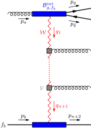
(a)

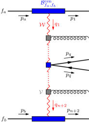
(b)

Figure 3: Structure of the matrix element for multijet production involving an extremal (a) or central (b) quark-antiquark pair.

Central $q\bar{q}$ production is depicted in figure 3(b) and corresponds to the configuration

$$f_{a}f_{b}\to f_{a}\cdot n_{1}g\cdot q\bar{q}\cdot(n-n_{1})g\cdot f_{b}.\\$$ (21)

The central production is described by an effective vertex $X_{\text{cen}}^{\mu\nu}$ that can be absorbed into the current contraction. The Born function then reads

$${\cal B}^{\text{cen}}_{f_{a},f_{b}}=(g_{s}^{2})^{4}\frac{K_{f_{a}}K_{f_{b}}}{4(N_{C}^{2}-1)}\|S_{f_{a}f_{b}\to f_{a}\cdots q\bar{q}\cdots f_{b}}\|^{2}\frac{1}{q_{1}^{2}q_{n+2}^{2}}$$ (22)

with the current contraction

$$\|S_{f_{a}f_{b}\to f_{a}\cdots q\bar{q}\cdots f_{b}}\|^{2}\equiv\|j^{a}\cdot X_{\text{cen}}\cdot j^{b}\|^{2}=\sum_{h_{a},h_{b}}|j_{\mu}^{h_{a}}(p_{1},p_{a})X_{\text{cen}}^{\mu\nu}j_{\nu}^{h_{b}}(p_{n+2},p_{b})|^{2},$$ (23)

where $X_{\text{cen}}^{\mu\nu}$ is derived in [5]. The $t$-channel momenta are given by

$$q_{i}=\begin{cases}p_{a}-\sum_{j=1}^{i}p_{i}&i\leq n_{1}+1\\ p_{a}-p_{q}-p_{\bar{q}}-\sum_{j=1}^{i}p_{i}&i>n_{1}+1\end{cases}.$$ (24)

2.3.2 W + jets production

If an additional leptonically decaying W boson is produced we have to distinguish between two cases. Similarly to the LL configurations, the W boson may couple to a fermion line associated with an incoming quark or antiquark. This causes a flavour change $f_{a}\to f_{a^{\prime}}$ or $f_{b}\to f_{b^{\prime}}$. Assuming without loss of generality the latter possibility the corresponding configurations read

$$gf_{b}\to{} Xq\bar{q}\cdot ng\cdot f_{b^{\prime}} (\text{extremal }q\bar{q}),$$ (25)

$$f_{a}f_{b}\to{} Xf_{a}\cdot n_{1}g\cdot q\bar{q}\cdot(n-n_{1})g\cdot f_{b^{\prime}} (\text{central }q\bar{q}),$$ (26)

where $X=l\bar{\nu}_{l}$ or $X=\bar{l}\nu_{l}$.

The Born functions for both configurations are obtained from the corresponding pure-jets Born functions in equations (19) and (22) by replacing the standard current $j^{\mu}(p_{b},p_{n+2})$ with the generalisation $j_{V}^{\mu}(p_{b},p_{\ell},p_{\bar{\ell}},p_{n+2})$ for the emission of a vector boson $V=W$, see equation (10).

The second possibility is a coupling of the W boson to the fermion line of the produced $q\bar{q}\mkern 1.0mu^{\prime}$, where now $q\neq q^{\prime}$. For extremal $q\bar{q}\mkern 1.0mu^{\prime}$ production, the Born function is obtained from equations (19) and (20) by replacing the current $j_{q\bar{q}}$ with a new effective current $j_{Wq\bar{q}^{\prime}}$. In complete analogy the central production is described by replacing $X_{\text{cen}}$ with a new effective vertex $X_{W\text{cen}}$ in equations (22), (23). Explicit results for $j_{Wq\bar{q}^{\prime}}$ and $X_{W\text{cen}}$ were obtained in [5].

3 Application: W + jets production

In order to demonstrate the recent additions to HEJ we now show in detail how to obtain a prediction for the production of a W boson with multiple jets. Specifically, we consider the process $pp\to(W^{-}\to e\bar{\nu}_{e})+\geq 2$ jets. The parameters are listed in table 2.

Collider energy		$\sqrt{s}=13$ TeV
Scales		$\mu_{r}=\frac{H_{T}}{2}$
		$\mu_{f}=\frac{H_{T}}{2}$
PDF set		CT18NLO
Electroweak input parameters		$G_{F}=1.3663787\cdot 10^{-5}\,\text{GeV}^{-2}$
		$m_{W}=80.385$ GeV
		$\Gamma_{W}=2.085$ GeV
		$m_{Z}=91.187$ GeV
		$\Gamma_{Z}=2.495$ GeV
Jet definition		anti-$k_{t}$ [19]
		$R=0.7$
		$p_{\perp}>20$ GeV

Table 2: Parameters used for the production of a leptonically decaying W boson with multiple jets.

3.1 Fixed-order input

In order to run ${\tt HEJ}$, we have to generate leading-order input events. Any generator producing event files in the Les Houches Event File (LHEF) [20] format can be used to this end. Here, we use Sherpa [21] with the following run card. The entries are explained in detail in the Sherpa documentation.

Run.dat

⬇

(run){

EVENTS 10000

EVENT_OUTPUT LHEF[events_W2j]

# collider beam

BEAM_1 2212

BEAM_ENERGY_1 6500

BEAM_2 2212

BEAM_ENERGY_2 6500

SCALES VAR{H_T2/4}

# PDF

PDF_LIBRARY LHAPDFSherpa

PDF_SET CT18NLO

MODEL SM

# electroweak parameters

EW_SCHEME 3

GF 1.1663787e-05

MASS[24] 80.385

WIDTH[24] 2.085

MASS[23] 91.187

WIDTH[23] 2.495

# massless charm quark

MASSIVE[4] 0

YUKAWA[4] 0.

MASS[4] 0.

# massless bottom quark

MASSIVE[5] 0

YUKAWA[5] 0.

MASS[5] 0.

ME_SIGNAL_GENERATOR Comix

EVENT_GENERATION_MODE Weighted

# disable everything beyond fixed order

FRAGMENTATION Off

YFS_MODE 0

MI_HANDLER None

SHOWER_GENERATOR None

CSS_MAXEM 0

BEAM_REMNANTS 0

}(run)

(processes){

Process 93 93 -> 24[a] 93 93

Decay 24[a] -> -11 12

Order (*,2)

End process

}(processes)

(selector){

# require 2 anti-kt jets with pt > 18 GeV and R = 0.7

FastjetFinder antikt 2 18. 0.0 0.7

}(selector)

Note that we have chosen a minimum jet transverse momentum of $18$ GeV instead of the $20$ GeV listed in table 2. The reason for this is that the HEJ resummation can change the transverse momenta of the jets slightly compared to the input leading-order events. It is therefore recommended to choose a minimum transverse momentum that is at least $10\%$ smaller in the fixed-order generation. It is also prudent to ensure that the final predictions do not change when choosing an even smaller value.

The contribution from events containing such “soft” jets with transverse momenta below the value required in the final analysis is numerically small. This means that a significant amount of computing time can be saved by generating two separate input event samples: one sample with low statistics in which each event contains at least one soft jet, and one large sample without any soft jets. We then apply resummation separately to each of the samples. Since the two samples cover distinct regions of the fixed-order phase space, the final prediction is simply the set of all generated events. For simplicity, we do not consider this optimisation in the following.

With the above Run.dat run card, an event file events_W2j.lhe can be generated by running

⬇

Sherpa

in the same directory. The generated events will contain exactly two jets, but it is straightforward to generate higher-multiplicity samples by increasing the required number of jets in FastjetFinder, adding the corresponding number of 93 entries to the Process final state, and adjusting the name of the output file in the EVENT_OUTPUT. HEJ can then be used to merge samples with different multiplicities. Typically, the contribution of higher jet multiplicities in the analysis will be decreasing, and it is often enough to consider at most four or five jets. One can save computing time at the price of sacrificing leading-order accuracy by using the HEJ fixed-order generator (HEJFOG) for high multiplicities. An example is shown in appendix A.

3.2 Resummation with HEJ

In addition to the fixed-order input, HEJ also requires a configuration file. A template config.yml is included in the HEJ source code. Adopting the current set of parameters from table 2 and enabling resummation for all supported NLL configurations we get

config_Wjets.yml

⬇

## Number of attempted resummation phase space points for each input event

trials: 10

resummation jets: # resummation jet properties

algorithm: antikt # jet clustering algorithm

R: 0.7 # jet R parameter

min pt: 20 # minimum jet transverse momentum

fixed order jets: # properties of input jets

min pt: 18

# by default, algorithm and R are like for resummation jets

## Treatment of the various event classes

## the supported settings are: reweight, keep, discard

## non-resummable events cannot be reweighted

event treatment:

FKL: reweight

# Enable resummation for NLL configurations

unordered: reweight

extremal qqbar: reweight

central qqbar: reweight

non-resummable: keep

## Central scale choice or choices

scales: H_T/2

## Selection of random number generator and seed

random generator:

name: mixmax

seed: 1

## Whether or not to include higher order logs

log correction: false

## Vacuum expectation value

vev: 246.2196508

## Properties of the weak gauge bosons

particle properties:

W:

mass: 80.385

width: 2.085

Z:

mass: 91.187

width: 2.495

Higgs:

mass: 125

width: 0.004165

We can now generate HEJ events and calculate the total resummed cross section. If HEJ is not installed, it can still be run using the Docker virtualisation software [22] and the following command.

⬇

docker run -v $PWD:$PWD -w $PWD hejdock/hej HEJ config_Wjets.yml events_W2j.lhe

If a HEJ installation is available, we can instead run

⬇

HEJ config_Wjets.yml events_W2j.lhe

If HEJ was compiled with support for Rivet [23], the generated events can be forwarded directly to the MC_WJETS analysis by adding the following lines to config_Wjets.yml before running HEJ:

⬇

analyses:

- rivet: MC_WJETS

output: HEJ_W2j

Another possibility is to create an output event file for manual analysis. After compiling HEJ with support for the HepMC 2 [24] format, we can add the following entry to config_Wjets.yml:

⬇

event output:

- HEJ_W2j.hepmc2

We can then run HEJ as before and feed the generated events into the MC_WJETS analysis with

⬇

rivet -a MC_WJETS -o HEJ_W2j.yoda HEJ_W2j.hepmc2

Results for higher jet multiplicities are obtained in the same way after adjusting the file names in the configuration files and run commands. To guarantee statistical independence it is also recommended to change the seed in config_Wjets.yml. To obtain a prediction that is inclusive in jet multiplicity, we combine the Rivet output with

⬇

yodastack -o HEJ_Wjets.yoda HEJ_W*j.yoda

Finally,

⬇

rivet-mkhtml HEJ_Wjets.yoda

produces analysis plots. As examples, we show the inclusive $N$-jet cross sections and the invariant mass distribution of the two hardest jets obtained from fixed-order input events with up to four jets in figure 4.

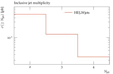
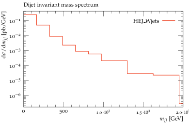
Figure 4: Inclusive $N$-jet cross sections (left) and dijet invariant mass spectrum (right) obtained with Sherpa and HEJ 2.1 for the production of a W boson with at least two jets.

4 Conclusions

This article accompanies the release of the event generator, HEJ 2.1 which provides predictions for hadronic colliders which contain contributions at all orders in $\alpha_{s}$ to achieve leading-logarithmic accuracy in $\hat{s}/p_{\perp}^{2}$. The output is given as exclusive events meaning that predictions can be obtained for arbitrary experimental cuts and analyses.

Here, after a brief outline of the general HEJ formalism, we have described the new extensions which have broadened the scope of the all-order predictions. Specifically, new matrix elements which allow for interference between channels with different assignments of effective $t$-channel momenta have been developed to give an accurate description of $pp\to(Z/\gamma^{*}\to\ell\bar{\ell})+\geq 2$ jets (section 2.2.2). Secondly, the full set of NLL contributions corresponding to processes which have no LL component have been incorporated through the derivation of necessary additional Born processes (section 2.3). These form a well-defined, gauge-invariant subset of the full NLL corrections.

Finally, we have provided a worked example explicitly showing all the steps necessary to generate predictions for $pp\to(W^{-}\to e\bar{\nu}_{e})+\geq 2$ jets.

Appendix A W + jets production with the HEJ fixed-order generator

The generation of fixed-order events with high jet multiplicities can become prohibitively expensive in computing time. In such cases the HEJ fixed-order generator (HEJFOG) can be used to quickly obtain results in the high-energy approximation. A typical use case is to produce HEJ input files with exact leading-order accuracy up to a given jet multiplicity as discussed in section 3.1 and supplement them with high-multiplicity event files produced with the HEJFOG.

As an example, we slightly modify the configuration file configFO.yml included in the HEJ source code to produce events for the process $pp\to(W^{-}\to e\bar{\nu}_{e})+5$ jets.

config_HEJFOG.yml

⬇

## Number of generated events

events: 10000

jets:

min pt: 18 # minimal jet pt, should be slightly below analysis cut

peak pt: 20 # peak pt of jets, should be at analysis cut

algorithm: antikt # jet clustering algorithm

R: 0.7 # jet R parameter

max rapidity: 5 # maximum jet rapidity

## Particle beam

beam:

energy: 6500

particles: [p, p]

## PDF ID for CT18NLO

pdf: 14400

## Scattering process

process: p p => Wm 5j

## Particle decays (multiple decays are allowed)

decays:

Wm: {into: [e-, nu_e_bar]}

## Fraction of events with two extremal emissions in one direction

## that contain an subleading emission e.g. unordered emission

subleading fraction: 0.05

## Allow different subleading configurations.

## By default all processes are allowed.

## This does not check if the processes are implemented in HEJ!

#

subleading channels:

- unordered

- central qqbar

- extremal qqbar

## Central scale choice

scales: H_T/2

## Event output files

event output:

- events_W5j.lhe

## Selection of random number generator and seed

random generator:

name: mixmax

seed: 5

## Vacuum expectation value

vev: 246.2196508

## Properties of the weak gauge bosons

particle properties:

W:

mass: 80.385

width: 2.085

Z:

mass: 91.187

width: 2.495

Higgs:

mass: 125

width: 0.004165

unweight:

sample size: 10000

max deviation: 0

To generate the event file events_W5j.lhe run

⬇

docker run -v $PWD:$PWD -w $PWD hejdock/hej HEJFOG config_HEJFOG.yml

when using the HEJ Docker container or

⬇

HEJFOG config_HEJFOG.yml

when using a local HEJ installation.

References

- [1] J. R. Andersen and J. M. Smillie, Constructing All-Order Corrections to Multi-Jet Rates, JHEP 1001 (2010) 039, [0908.2786].
- [2] J. R. Andersen and J. M. Smillie, The Factorisation of the t-channel Pole in Quark-Gluon Scattering, Phys.Rev. D81 (2010) 114021, [0910.5113].
- [3] J. R. Andersen and J. M. Smillie, Multiple Jets at the LHC with High Energy Jets, JHEP 1106 (2011) 010, [1101.5394].
- [4] J. R. Andersen, T. Hapola, A. Maier and J. M. Smillie, Higgs Boson Plus Dijets: Higher Order Corrections, JHEP 09 (2017) 065, [1706.01002].
- [5] J. R. Andersen, J. A. Black, H. M. Brooks, E. P. Byrne, A. Maier and J. M. Smillie, Combined subleading high-energy logarithms and NLO accuracy for W production in association with multiple jets, JHEP 04 (2021) 105, [2012.10310].
- [6] ATLAS collaboration, G. Aad et al., Measurement of dijet production with a veto on additional central jet activity in collisions at TeV using the ATLAS detector, JHEP 09 (2011) 053, [1107.1641].
- [7] CMS collaboration, S. Chatrchyan et al., Measurement of the inclusive production cross sections for forward jets and for dijet events with one forward and one central jet in collisions at TeV, JHEP 06 (2012) 036, [1202.0704].
- [8] CMS collaboration, S. Chatrchyan et al., Ratios of dijet production cross sections as a function of the absolute difference in rapidity between jets in proton-proton collisions at TeV, Eur. Phys. J. C 72 (2012) 2216, [1204.0696].
- [9] ATLAS collaboration, G. Aad et al., Measurements of jet vetoes and azimuthal decorrelations in dijet events produced in collisions at using the ATLAS detector, Eur. Phys. J. C 74 (2014) 3117, [1407.5756].
- [10] J. R. Andersen, T. Hapola and J. M. Smillie, W Plus Multiple Jets at the LHC with High Energy Jets, JHEP 1209 (2012) 047, [1206.6763].
- [11] D0 collaboration, V. M. Abazov et al., Studies of W boson plus jets production in collisions at TeV, Phys. Rev. D 88 (2013) 092001, [1302.6508].
- [12] ATLAS collaboration, G. Aad et al., Measurements of the W production cross sections in association with jets with the ATLAS detector, Eur. Phys. J. C 75 (2015) 82, [1409.8639].
- [13] J. R. Andersen, J. J. Medley and J. M. Smillie, plus multiple hard jets in high energy collisions, JHEP 05 (2016) 136, [1603.05460].
- [14] J. R. Andersen, V. Del Duca and C. D. White, Higgs Boson Production in Association with Multiple Hard Jets, JHEP 02 (2009) 015, [0808.3696].
- [15] J. R. Andersen, T. Hapola, M. Heil, A. Maier and J. M. Smillie, Higgs-boson plus Dijets: Higher-Order Matching for High-Energy Predictions, JHEP 08 (2018) 090, [1805.04446].
- [16] J. R. Andersen, J. D. Cockburn, M. Heil, A. Maier and J. M. Smillie, Finite Quark-Mass Effects in Higgs Boson Production with Dijets at Large Energies, JHEP 04 (2019) 127, [1812.08072].
- [17] J. R. Andersen, T. Hapola, M. Heil, A. Maier and J. Smillie, HEJ 2: High Energy Resummation for Hadron Colliders, Comput.Phys.Commun. 245 (2019) , [1902.08430].
- [18] L. N. Lipatov, Reggeization of the Vector Meson and the Vacuum Singularity in Nonabelian Gauge Theories, Sov. J. Nucl. Phys. 23 (1976) 338–345.
- [19] M. Cacciari, G. P. Salam and G. Soyez, The anti- jet clustering algorithm, JHEP 04 (2008) 063, [0802.1189].
- [20] J. Alwall et al., A Standard format for Les Houches event files, Comput. Phys. Commun. 176 (2007) 300–304, [hep-ph/0609017].
- [21] Sherpa collaboration, E. Bothmann et al., Event Generation with Sherpa 2.2, SciPost Phys. 7 (2019) 034, [1905.09127].
- [22] “Docker.”
- [23] C. Bierlich et al., Robust Independent Validation of Experiment and Theory: Rivet version 3, SciPost Phys. 8 (2020) 026, [1912.05451].
- [24] M. Dobbs and J. B. Hansen, The HepMC C++ Monte Carlo event record for High Energy Physics, Comput. Phys. Commun. 134 (2001) 41–46.
- [25] M. Cacciari, G. P. Salam and G. Soyez, FastJet User Manual, Eur. Phys. J. C 72 (2012) 1896, [1111.6097].
- [26] A. Buckley, J. Ferrando, S. Lloyd, K. Nordström, B. Page, M. Rüfenacht et al., LHAPDF6: parton density access in the LHC precision era, Eur. Phys. J. C 75 (2015) 132, [1412.7420].
- [27] J. A. M. Vermaseren, New features of FORM, math-ph/0010025.