A novel event generator for the automated simulation of neutrino scattering

Abstract

An event generation framework is presented that enables the automatic simulation of events for next-generation neutrino experiments in the Standard Model or extensions thereof. The new generator combines the calculation of the leptonic current based on an automated matrix element generator, and the computation of the hadronic current based on a state-of-the-art nuclear physics model. The approach is validated in Standard-Model simulations for electron scattering and neutrino scattering. Furthermore, the first fully-differential neutrino trident production results are shown in the quasielastic region.

I Introduction

Neutrino physics is entering an era of precision measurements. The development of the Deep Underground Neutrino Experiment (DUNE) Abi et al. (2021, 2020) and of the Hyperkamiokande (HyperK) Abe et al. (2018) detector will allow us to probe neutrino interactions to unprecedented precision, and will allow for tests of beyond the Standard Model (BSM) scenarios such as proton decay, sterile neutrinos and heavy neutral leptons, as well as rare Standard Model (SM) processes such as neutrino tridents Abi et al. (2021); Yano (2021). The excess of electron-like events in measurements at LSND Aguilar et al. (2001) and MiniBooNE Aguilar-Arevalo et al. (2007, 2009, 2010, 2013, 2018, 2021) has demonstrated the need for a toolkit which allows the physics community to quickly test different hypotheses against experimental data. While calculations can be done on a case-by-case basis, such as in Refs. Gninenko (2009); McKeen and Pospelov (2010); Gninenko (2011); Dib et al. (2011); Gninenko (2012); Masip et al. (2013); Ballett et al. (2017); Magill et al. (2018); Fischer et al. (2020); Bertuzzo et al. (2018a, b); Ballett et al. (2019a); Argüelles et al. (2019); Ballett et al. (2019b, 2020); Abdullahi et al. (2020); Abdallah et al. (2020a, b); de Gouvêa et al. (2020); Dentler et al. (2020); Chang et al. (2021), a dedicated analysis for each new physics model becomes impractical when there is a wealth of ideas and a large number of measurements that present simultaneous constraints, such as the recent MicroBooNE results Abratenko . In such cases an end-to-end simulation should be attempted, starting with the Lagrangian of the underlying new physics hypothesis, and leading to particle-level events that are generated fully differentially in the many-particle phase space by means of Monte-Carlo methods. In addition, it must be possible to implement this simulation pipeline as part of experimental analysis frameworks, such that detector effects can be fully included.

The accurate simulation of particle-level events based on an underlying physics model has been a cornerstone of high-energy physics experiments for many decades. In the context of Large Hadron Collider (LHC) physics, the problem of an end-to-end simulation pipeline has been encountered long ago, and it was successfully addressed through the development of FeynRules Christensen and Duhr (2009); Alloul et al. (2014), specific event generator interfaces Christensen et al. (2011, 2012) and eventually the UFO file format Degrande et al. (2012). A complete toolchain has been developed, starting with the conversion of the Lagrangian to Feynman rules Christensen and Duhr (2009); Alloul et al. (2014), followed by the perturbative calculation of cross sections and event simulation by Amegic Krauss et al. (2002), Comix Gleisberg and Höche (2008), Herwig++ Bähr et al. (2008); Bellm et al. (2016), MadGraph Alwall et al. (2014) or Whizard Kilian et al. (2007), and finally leading to particle-level event simulation with Herwig Bähr et al. (2008); Bellm et al. (2016), Pythia Sjöstrand et al. (2006, 2015) or Sherpa Gleisberg et al. (2009); Bothmann et al. (2019). The flexibility of the aforementioned tools plays a major role in the exploration of model and parameter space by the LHC experiments. In anticipation of similar needs at next generation neutrino experiments, we develop a simulation framework that allows for the generation of particle-level events in arbitrary new physics models, while at the same time appropriately including nuclear effects. We validate our new framework in Standard Model electron- and neutrino-nucleus scattering. We also calculate the first results for fully differential neutrino trident production in the quasielastic region.

This manuscript is structured as follows: Section II presents an introduction to the problem of neutrino-nucleus scattering and lays out the general framework for the calculation. Section III introduces our technique to compute the leptonic tensor, and Sec. IV reviews the techniques for phase-space integration. Section V outlines the computation of the hadronic tensor. First numerical results are presented in Sec. VI and Sec. VII contains an outlook.

II Theory Overview

In neutrino experiments, the majority of events of interest can be described via an exchange of a single gauge boson. In this case, the differential cross section factorizes as:

$$\frac{{\rm d}\sigma}{{\rm d}\Omega}\propto L_{\mu\nu}W^{\mu\nu},$$ (1)

where $L_{\mu\nu}\,(W^{\mu\nu})$ is the leptonic (hadronic) tensor.

The leptonic tensor can be calculated using methods developed for collider event generation and will be discussed in detail in Sec. III. On the other hand, when dropping spin dependent terms, the hadronic tensor can be written using the most general Lorentz structure as:

$$W^{\mu\nu}=\left(-g^{\mu\nu}+\frac{q^{\mu}q^{\nu}}{q^{2}}\right)W_{1}+\frac{\hat{p}_{a}^{\mu}\hat{p}_{a}^{\nu}}{p_{a}\cdot q}W_{2}-i\epsilon^{\mu\nu\alpha\beta}\frac{q_{\alpha}p_{a\beta}}{2p_{a}\cdot q}W_{3},$$ (2)

where $p_{a}$ is the momentum of the initial nucleon, $q$ is the momentum of the probe, $\hat{p}_{a}^{\mu}=p_{a}^{\mu}-\frac{p_{a}\cdot q}{q^{2}}q^{\mu}$, $Q^{2}=-q^{2}$, and $W_{i}$ are the nuclear structure functions.

Factorizing the differential cross section in this manner allows us to separate the BSM effects that would be dominant in the leptonic tensor from the complicated nuclear physics calculations of the hadronic tensor. Moreover, neutrino event generators have already implemented many nuclear models into their codes Juszczak et al. (2006); Andreopoulos (2009); Hayato (2009); Buss et al. (2012), making the calculation of $W^{\mu\nu}$ a straightforward process. Therefore, we can leverage the work done on the nuclear side to make accurate predictions for different BSM scenarios at DUNE, HyperK, MicroBooNE, and MiniBooNE.

While Eq. (1) works when a single type of gauge boson exchange dominates the total cross section (i.e. the photon for electron scattering, the $W$ boson for charged-current neutrino scattering, and the $Z$ boson for neutral-current neutrino scattering), this approximation breaks down when interference is important. In this case, the differential cross section can be obtained through an extended factorization formula that reads

$$\frac{{\rm d}\sigma}{{\rm d}\Omega}=\sum_{i,j}L^{(ij)}_{\mu\nu}W^{(ij){\mu\nu}},$$ (3)

where the sum over $i,j$ is for each allowed boson in the process. For example, adding in the $Z$ boson contributions to electron scattering would result in

$$\frac{{\rm d}\sigma}{{\rm d}\Omega}=L^{(\gamma\gamma)}_{\mu\nu}W^{(\gamma\gamma){\mu\nu}}+L^{(\gamma Z)}_{\mu\nu}W^{(\gamma Z){\mu\nu}}+L^{(Z\gamma)}_{\mu\nu}W^{(Z\gamma){\mu\nu}}+L^{(ZZ)}_{\mu\nu}W^{(ZZ){\mu\nu}}.$$ (4)

This formulation of the problem quickly becomes unwieldy as the number of allowed bosons in the process increases. In these situations, it is better to write the differential cross section as the square of a product of leptonic and hadronic currents:

$$\frac{{\rm d}\sigma}{{\rm d}\Omega}=\bigg{|}\sum_{i}L^{(i)}_{\mu}W^{(i)\mu}\bigg{|}^{2},$$ (5)

where the interference terms are automatically included by taking the square of the sum of amplitudes. In this work, we will use Eq. (5) for our calculations, but in the cases when the nuclear physics cannot be written as a current, we provide the option to work with the leptonic tensor in Eq. (3).

The BSM calculations we intend to automate involve only the leptonic current and are independent of the exact nuclear model. We will therefore focus on the quasielastic region in this work for concreteness. Specifically, the hadronic current will be computed in the impulse approximation (IA), using the spectral function formalism as discussed in Refs. Benhar et al. (2008); Rocco et al. (2019a). In this approximation, the nuclear current can be expressed as a sum of one-body currents, and the nuclear final state can be written as a struck nucleon and an $A-1$ spectator nuclear remnant. Given the initial nuclear ground state $\lvert\psi_{0}^{A}\rangle$ and the nuclear final state $\langle\psi_{f}^{A}\rvert$, the current operator can be rewritten through the insertion of a complete set of states ($\sum_{k}\lvert k\rangle\langle k\rvert$) in the IA as:

$$W^{\mu}=\langle\psi_{f}^{A}\rvert\mathcal{J}^{\mu}\lvert\psi_{0}^{A}\rangle\rightarrow\sum_{k}\left[\langle\psi_{f}^{A-1}\rvert\otimes\langle k\rvert\right]\rvert\psi_{0}^{A}\rangle\langle p_{a}+q\rvert\sum_{i}\mathcal{J}_{i}^{\mu}\lvert k\rangle,$$ (6)

where $\mathcal{J}^{\mu}$ is the current operator of the boson probing the nucleus, and $\mathcal{J}_{i}^{\mu}$ is the current operator contribution from the $i^{\rm th}$ nucleon in the IA. The incoherent contribution to the hadronic tensor can then be calculated as:

$$W^{\mu\nu}=\int\frac{{\rm d}^{3}p_{a}}{(2\pi)^{3}}{\rm d}E\,S(\mathbf{p_{a}},E_{r})\sum_{i}\langle p_{a}\rvert\mathcal{J}_{i}^{\mu}\lvert p_{a}+q\rangle\langle p_{a}+q\rvert\mathcal{J}_{i}^{\nu\dagger}\lvert k\rangle\delta\left(\omega-E_{r}+m-E^{\prime}\right),$$ (7)

where $\omega$ is the lepton energy loss, $E_{r}$ is the excitation energy of the $A-1$ nucleon system, $E^{\prime}$ is the outgoing nucleon energy and $S(\mathbf{p}_{a},E_{r})$ is the spectral function which gives the probability of removing a nucleon with three-momentum $\mathbf{p}_{a}$ and excitation energy $E_{r}$. The spectral functions of finite nuclei have been obtained using different nuclear many-body approaches Dickhoff and Charity (2019); Dickhoff and Atkinson (2020); Barbieri and Hjorth-Jensen (2009); Benhar et al. (1994); Sick et al. (1994). In particular, those computed within the correlated-basis function (CBF) theory, Self Consistent Green’s Function (SCGF), and variational Monte Carlo (VMC) methods have yielded consistent inclusive lepton-scattering cross sections on different nuclear targets Rocco et al. (2019a); Rocco and Barbieri (2018); Andreoli et al. (2021); Ankowski et al. (2015). The CBF spectral function used in this work is given as a sum of two terms. The first term, which describes the low excitation energy and momentum region, uses as input spectroscopic factors extracted from ($e,e^{\prime}p$) scattering measurements. The second term accounts for unbound states of the $A-1$ spectator system in which at least one of the spectator nucleons is in a continuum state. This contribution is obtained by folding the correlation component of the nuclear matter spectral function obtained within the CBF theory with the the density profile of the nucleus Benhar et al. (1989).

The nuclear one-body current operator can be expressed in general as the sum of the vector (V) and axial-vector (A) terms given as:

$$\mathcal{J}^{\mu} =\left(\mathcal{J}_{V}^{\mu}+\mathcal{J}_{A}^{\mu}\right)$$

$$\mathcal{J}^{\mu}_{V} =\gamma^{\mu}\mathcal{F}^{a}_{1}+i\sigma^{\mu\nu}q_{\nu}\frac{\mathcal{F}^{a}_{2}}{2M}$$ (8)

$$\mathcal{J}^{\mu}_{A} =-\gamma^{\mu}\gamma_{5}\mathcal{F}^{a}_{A}-q^{\mu}\gamma_{5}\frac{\mathcal{F}^{a}_{P}}{M},$$

where $\mathcal{F}^{a}_{i}$ are the process dependent nuclear form factors for the exchange of the boson $a$ and $M$ is the nucleon mass. Since the pseudo-scalar form factor ($\mathcal{F}^{a}_{P}$) is multiplied by the mass of the outgoing lepton in the cross section, we neglect the contribution from it in this work. The values for the form factors considered here are detailed in Sec. V.

III Calculation of the Leptonic Current

Employing a dedicated version of the general-purpose event generator Sherpa Gleisberg et al. (2004, 2009); Bothmann et al. (2019), we construct an interface to the Comix matrix element generator Gleisberg and Höche (2008) to extract the leptonic current. In Comix, the matrix element is computed using the color-dressed Berends-Giele recursive relations Duhr et al. (2006), which can be understood as a Dyson-Schwinger based technique Kanaki and Papadopoulos (2000); Mangano et al. (2003). In this technique, the full tree-level scattering amplitude is determined from off-shell currents which are composed of all sub-diagrams connecting a certain sub-set of external particles. These currents depend on the momenta $p_{1},\ldots,p_{n}$ of external particles $1,\ldots,n$, and on their helicities and colors.

The off-shell currents satisfy the recursive relations

$$J_{\alpha}(\pi)=P_{\alpha}(\pi)\,\sum\limits_{\mathcal{V}_{\alpha}^{\;\alpha_{1},\,\alpha_{2}}}\sum\limits_{\mathcal{P}_{2}(\pi)}\mathcal{S}(\pi_{1},\pi_{2})\;\mathcal{V}_{\alpha}^{\,\alpha_{1},\,\alpha_{2}}(\pi_{1},\pi_{2})\,J_{\alpha_{1}}(\pi_{1})J_{\alpha_{2}}(\pi_{2})\;,$$ (9)

where, $P_{\alpha}(\pi)$ denotes a propagator, which depends on the particle type $\alpha$ and the set of particles, $\pi$. The term $\mathcal{V}_{\alpha}^{\,\alpha_{1},\alpha_{2}}(\pi_{1},\pi_{2})$ represents a vertex, which depends on the particle types $\alpha$, $\alpha_{1}$ and $\alpha_{2}$ and the decomposition of the set of particle labels, $\pi$, into disjoint subsets $\pi_{1}$ and $\pi_{2}$. The quantity $\mathcal{S}(\pi_{1},\pi_{2})$ is the symmetry factor associated with the decomposition of $\pi$ into $\pi_{1}$ and $\pi_{2}$ Gleisberg and Höche (2008). Superscripts refer to incoming particles at the vertex, subscripts to outgoing particles. The sums run over all vertices in the interaction model and over all unordered partitions $\mathcal{P}_{2}$ of the set $\pi$ into two disjoint subsets. Since we will use the above recursion only to compute the leptonic current, we can suppress color indices. Helicity labels are implied. The initial currents $J_{\alpha_{i}}(p_{i})$ can be determined based on the spin of the $i^{\text{th}}$ external particle. The external currents are given by:

$$J_{\alpha}(p_{i})=\begin{cases}1&\text{spin}=0\\ u(p_{i})\ \text{or}\ v(p_{i})&\text{spin}=1/2\\ \epsilon_{\alpha}(p_{i},k)&\text{spin}=1\end{cases},$$ (10)

where $u(p_{i})$ and $v(p_{i})$ are the solutions to the Dirac equation, $\epsilon_{\alpha}$ is the polarization vector, and $k$ is an auxiliary vector to define the polarization.

A complete list of interaction vertices for the Standard Model can be found in Ref. Gleisberg and Höche (2008). For completeness, we also list the nontrivial expressions for the natively implemented Lorentz structures in App. A. Comix allows to include Feynman rules for nearly arbitrary new physics scenarios into Eq. (9) by means of a generic interface to the UFO file format Degrande et al. (2012), and an automated generator for the Lorentz (and color) structures Höche et al. (2015); Krauss et al. (2017). This extension of Comix to BSM calculations also discusses the extension of Eq. (9) from containing only 3-point vertices to arbitrary $N$-point vertices. The generation of UFO files can be accomplished through the use of the FeynRules program Christensen and Duhr (2009); Alloul et al. (2014), which can take any Lagrangian and obtain the needed Feynman rules for tree-level calculations.

In order to compute the leptonic current needed to evaluate Eq. (1), we introduce point-like nucleons into the theory, which act as auxiliary particles that are needed only for bookkeeping purposes and to construct a formally complete scattering amplitude. The off-shell currents coupling to these nucleons are then used to define the leptonic current or the leptonic tensor as

$$\begin{split}L_{\mu}^{(i)}(1,\ldots,m)=&\;J^{(i)}_{\mu}(1,\ldots,m)\;,\\ L_{\mu\nu}^{(ij)}(1,\ldots,m)=&\;J^{(i)}_{\mu}(1,\ldots,m)J^{(j)\dagger}_{\nu}(1,\ldots,m)\;,\end{split}$$ (11)

where the particles $1,\ldots,m$ are the non strongly interacting particles that contribute to the leptonic current.

Through the use of the recursion relations, and the interface with UFO files generated from FeynRules, this generator can calculate almost any leptonic current that may be of interest. The only limitations on the leptonic currents that can be calculated are: can not currently handle any spin $>$ 1 particles, can not have any color charged particles, only spin-1 particles can probe the nucleus, and only tree-level diagrams can be calculated. Of these limitations, only the exclusion of the color charged particles can not be resolved with future work. Allowing color charged particles to interact with the nucleus breaks the assumption that the degrees of freedom in QCD are protons and neutrons. Implementing other probes of the nucleus involves updating the nuclear physics to include the appropriate form factors for the different spin probes. Handling particles with spin $>$ 1 requires implementing the needed external particle states and appropriate propagators. The automation of one-loop diagrams has been discussed in detail in Refs. Hirschi et al. (2011); Denner et al. (2018); Buccioni et al. (2019).

IV Phase-space integration

We employ the recursive phase-space generation techniques of Ref. Byckling and Kajantie (1969) in combination with the multi-channel method of Ref. Kleiss and Pittau (1994) and the adaptive multi-dimensional integration algorithm Vegas Lepage (1980) in order to perform the phase-space integrals. Considering a $2\to n$ scattering process with incoming particles $a$ and $b$ and outgoing particles $1\ldots n$, the $n$-particle differential phase space element reads

$${\rm d}\Phi_{n}(a,b;1,\ldots,n)=\left[\,\prod\limits_{i=1}^{n}\frac{{\rm d}^{4}p_{i}}{(2\pi)^{3}}\,\delta(p_{i}^{2}-m_{i}^{2})\Theta(p_{i0})\,\right]\,(2\pi)^{4}\delta^{(4)}\left(p_{a}+p_{b}-\sum_{i=1}^{n}p_{i}\right)\;,$$ (12)

where $p_{i}$ and $m_{i}$ are the momentum and on-shell masses of outgoing particles, respectively.

For concreteness, consider the $2\to 2$ process $l+{}^{12}C\to l^{\prime}+N+X$ in the quasielastic regime. In this case, we not only have to consider the final state lepton and nucleon, but also the initial state of the system. In the quasielastic regime, the initial momentum of the nucleon can be generated by considering an isotropic three-momentum and a removal energy of the nucleon inside the nucleus. Furthermore, if the lepton is not monochromatic, then the momentum of the lepton can be generated according to the initial flux. Putting all the components together, the full differential phase space element is given as ${\rm d}\Phi_{2}(a,b;1,2){\rm d}^{3}\mathbf{p}_{a}{\rm d}E_{r}{\rm d}^{3}\mathbf{p}_{b}$, where ${\rm d}\Phi_{2}(a,b;1,2)$ is given in Eq. (12), $\mathbf{p}_{a}(E_{r})$ is the three-momentum (removal energy) of the initial nucleon, and $\mathbf{p}_{b}$ is the three-momentum of the initial lepton. This process will proceed through a $t$-channel exchange of a gauge boson. Therefore, it is efficient to rewrite the two-body final state phase space such that it appropriately samples a $t$-channel momentum distribution as:

$${\rm d}\Phi_{2}(a,b;1,2)=\frac{\lambda\left(s_{ab},s_{1},s_{2}\right)}{16\pi^{2}2s_{ab}}\,{\rm d}\cos\theta_{1}{\rm d}\phi_{1},$$ (13)

where $\theta_{1}(\phi_{1})$ is the polar (azimuthal) angle with respect to the axis formed by $p_{a}+p_{b}$. Here we have introduced the Källen function:

$$\lambda^{2}\left(s_{a},s_{b},s_{c}\right)={\left(s_{a}-s_{b}-s_{c}\right)^{2}-4s_{b}s_{c}},$$ (14)

where $s_{i}$ denotes the invariant mass of the particles $i$. The differential phase-space element ${\rm d}^{3}\mathbf{p}_{a}$ can be rewritten as:

$${\rm d}^{3}\mathbf{p}_{a}=|\mathbf{p}_{a}|^{2}{\rm d}\mathbf{p}_{a}{\rm d}\cos\theta_{a}{\rm d}\phi_{a},$$ (15)

where $E_{r}$ is the removal energy, $\theta_{a}(\phi_{a})$ is the polar (azimuthal) angle with respect to the beam direction, and the energy of the nucleon is given as $E_{a}=m_{N}-E_{r}$ to convert the quasielastic energy conservation $\delta$-function given in Eq. (7) to $\delta\left(E_{a}+E_{b}-E_{1}-E_{2}\right)$, which is consistent with the energy conservation of Eq. (12). The initial distribution for the lepton depends on the experiment being considered, and is typically given as a probability distribution given some initial momentum (and position in the case of fluxes from NuMI beam simulations Adamson et al. (2016)). Events can be generated according to this probability distribution with various MC techniques. In this work, we consider only monochromatic beams, so details of these methods are left to a future work.

To generalize the phase-space integration to higher multiplicities, we follow Ref. James , factorizing Eq. (12) as

$${\rm d}\Phi_{n}(a,b;1,\ldots,n)={\rm d}\Phi_{n-m+1}(a,b;\pi,m+1,\ldots,n)\,\frac{{\rm d}s_{\pi}}{2\pi}\,{\rm d}\Phi_{m}(\pi;1,\ldots,m)\;.$$ (16)

In this context, $\pi=\{1,\ldots,m\}$ corresponds to a subset of particle indices, similar to the notation in Sec. III. We use overlined letters to denote the missing subset, e.g. $\overline{\alpha}=\{a,b,1,\ldots,n\}\setminus\alpha$. Equation (16) allows the decomposition of the complete phase space into building blocks corresponding to the propagator-like term ${\rm d}s_{\pi}/(2\pi)$ and the $s$- and $t$-channel decay processes

$$\begin{split}S_{\pi}^{\,\rho,\pi\setminus\rho}&=\frac{\lambda(s_{\pi},s_{\rho},s_{\pi\setminus\rho})}{16\pi^{2}\,2\,s_{\pi}}\;{\rm d}\cos\theta_{\rho}\,{\rm d}\phi_{\rho}\;,\\ T_{\alpha,b}^{\,\pi,\overline{\alpha b\pi}}&=\frac{\lambda(s_{\alpha b},s_{\pi},s_{\;\overline{\alpha b\pi}})}{16\pi^{2}\,2s_{\alpha b}}\;{\rm d}\cos\theta_{\pi}\,{\rm d}\phi_{\pi}\;,\\ \end{split}$$ (17)

where $T_{\alpha,b}^{\,\pi,\overline{\alpha b\pi}}$ is the same function as in Eq. (13). In addition, an overall factor of $(2\pi)^{4}\,{\rm d}^{4}p_{\,\overline{\alpha b}}\;\delta^{(4)}(p_{\alpha}+p_{b}-p_{\,\overline{\alpha b}})$ guarantees four-momentum conservation. The basic idea of Ref. Byckling and Kajantie (1969) is to match the indices in the virtuality integrals of Eq. (16) and the lower left indices in the $T$ functions to indices of $t$-channel currents in the hard matrix element. In this manner, one obtains an optimal integrator for a particular Feynman diagram in a scalar theory that contains propagators with all these indices. An optimal integrator for all scalar diagrams can then be constructed using the multi-channel technique Kleiss and Pittau (1994). Finally, the spin dependence of the hard matrix element can be mapped out more carefully with the help of adaptive MC algorithms Lepage (1978); Bothmann et al. (2020); Gao et al. (2020).

V Nuclear Matrix Element Interface

While the UFO file is extremely flexible, it is missing a way to easily define the nuclear form factors involved within the interaction. We propose to use an extension to the UFO file format that provides a way to consistently interface with the form factors used in the neutrino event generators and other neutrino-nucleus interaction codes. This extension will only be valid as long as the Conserved Vector Current (CVC) hypothesis is valid. The CVC provides a method to relate the vector form factor for an arbitrary model to the electromagnetic form factors ($F_{1},F_{2}$). The electomagnetic form factors $F_{1}$ and $F_{2}$ can be defined in terms of the electric and magnetic form factors as:

$$F_{1}^{p,n} =\frac{G_{E}^{p,n}+\tau G_{M}^{p,n}}{1+\tau}$$

$$F_{2}^{p,n} =\frac{G_{E}^{p,n}-G_{M}^{p,n}}{1+\tau},$$ (18)

with $\tau=-q^{2}/(2M)^{2}$. In this work, we consider the Kelly parameterization for the electric and magnetic form factors Kelly (2004).

Additionally, we will consider a global axial-vector form factor as well. While it is straightforward to implement any form factor, such as the “z-expansion” Meyer et al. (2016), we choose to use the dipole parameterization to allow for a fair comparison to Ref. Rocco et al. (2019a). The standard dipole parameterization is given as

$$F_{A}=\frac{g_{A}}{(1-q^{2}/M_{A}^{2})^{2}},$$ (19)

where the nucleon axial-vector coupling constant is taken to be $g_{A}=1.2694$ and the axial mass is taken to be $M_{A}$ = 1.0 GeV. Studying the impact of different parameterizations of the axial-vector form factor are beyond the scope of this work.

The form factors for an arbitrary process can be expressed in the form factors given above through the use of their isospin dependent interactions. Here we work out the form factors for the Standard Model photon, $Z$ boson, and $W$ boson, but the process can be applied similarly to any BSM scenario. Since the form factors are defined in terms of the coupling to the photon, the photon form factors ($\mathcal{F}^{\gamma}_{i}$; see Eq. (II)) are straightforward, and given as:

$$\mathcal{F}^{\gamma(p,n)}_{i}=F^{p,n}_{i},\quad\quad\mathcal{F}^{\gamma}_{A}=0.$$ (20)

The $W^{\pm}$ boson couples via isospin through the $\tau^{\pm}$ operator, which leads to the form factors:

$$\mathcal{F}^{W(p,n)}_{i}=F^{p}_{i}-F^{n}_{i},\quad\quad\mathcal{F}^{W}_{A}=F_{A}.$$ (21)

The $Z$ boson also couples via isospin, and the form factors are

$$\mathcal{F}_{i}^{Z(p)} =\left(\frac{1}{2}-2\sin^{2}\theta_{W}\right)F_{i}^{p}-\frac{1}{2}F_{i}^{n},\quad\quad\mathcal{F}_{A}^{Z(p)}=\frac{1}{2}F_{A},$$

$$\mathcal{F}_{i}^{Z(n)} =\left(\frac{1}{2}-2\sin^{2}\theta_{W}\right)F_{i}^{n}-\frac{1}{2}F_{i}^{p},\quad\quad\mathcal{F}_{A}^{Z(n)}=-\frac{1}{2}F_{A},$$ (22)

where $\sin\theta_{W}$ is the weak mixing angle. We leave the examples of working out the form factors for specific BSM scenarios to a future work.

VI Results

We consider the processes of electron and neutrino scattering off Carbon, and neutrino trident production off Carbon. The electron scattering and neutrino scattering are used as a means to validate the code. The trident production is the first fully-differential calculation of tridents in the quasielastic region using nuclear spectral functions, to demonstrate the ability to extend the predictions beyond $2\to 2$ processes. For simplicity, we only consider a monochromatic beam for the incoming particle, but it is straightforward to include appropriate fluxes. Additionally, we do not include any final state interaction effects, which are known to shift the location of the peak of the distribution, reduce the height of the peak and broaden the tails of the distribution. For all the calculations, we set our electroweak parameters in the $(\alpha,G_{F},M_{Z})$-scheme, and the values are chosen as $\alpha=1/137$, $G_{F}=1.16637\times 10^{-5}$ GeV^-2, and $M_{Z}=91.1876$ GeV. Throughout the calculations, all leptons are considered massless particles. Furthermore, we include the full propagator and do not take the infinite mass limit for the contributions from $W$ or $Z$ bosons. This differs from previous works in which the four-point Fermi interactions are used to model the neutrino-nucleus interactions.

VI.1 Electron Scattering

There is a plethora of electron scattering data on a Carbon target that has been collected. Here we compare to a select few experimental results, along with the predictions based on Ref. Rocco et al. (2019b). The data is the double differential cross section in solid angle and the energy transfer ($\omega$) versus the energy transfer to the nucleus.

First, we consider the electron scattering off Carbon with an electron beam energy of 961 MeV and 37.5 degrees scattering angle Sealock et al. (1989). The comparison between the data, the results based on Ref. Rocco et al. (2019b), and our work can be seen in Fig. 1. We observe that the calculation is consistent with the original theory calculation. Furthermore, the difference in the quasielastic peak region between the theory calculation and the data can be explained by including final state interaction effects, as shown in Ref. Rocco et al. (2019b). The high energy transfer tail can be explained through the inclusion of two-body currents, resonance production, and deep-inelastic scattering Rocco et al. (2019b).

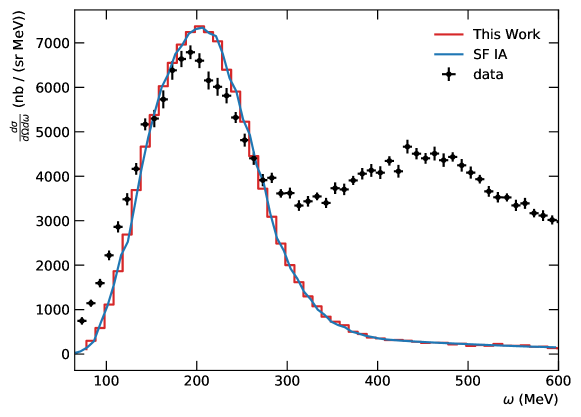
Figure 1: A comparison between our calculation, the data from Ref. Sealock et al. (1989), and the theory calculation based on Ref. Rocco et al. (2019b) for a 961 MeV electron scattering off Carbon at an angle of 37.5 degrees. The two theory calculations are consistent with each other, and the difference with the data can be explained by including final state interaction effects.

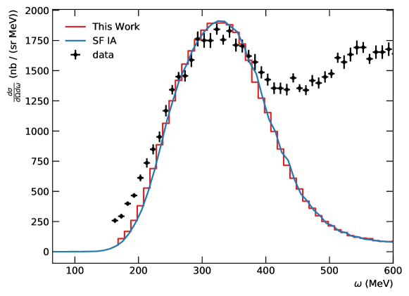
Figure 2: A comparison between our calculation, the data from Ref. Sealock et al. (1989), and the theory calculation based on Ref. Rocco et al. (2019b) for a 1300 MeV electron scattering off Carbon at an angle of 37.5 degrees. The two theory calculations are consistent with each other, and the difference with the data can be explained by including final state interaction effects.

Figure 2 displays the comparison between the two theory approaches and data for electron scattering off Carbon with an electron beam energy of 1300 MeV and 37.5 degrees scattering angle Sealock et al. (1989). Again, we observe that the two theory calculations are consistent. There is an overall agreement between the theory prediction based on Ref. Rocco et al. (2019b) and the data in the quasielastic region, the small difference at low $\omega$ has to be ascribed to final state interaction effects as in Fig. 2. These can be accounted for as demonstrated in Ref. Rocco et al. (2019b) but their inclusion is beyond the scope of this work.

VI.2 Neutrino Scattering

For neutrino scattering, we consider both neutrino and anti-neutrino beams. Since there are no high-energy monochromatic beams of neutrinos, we only compare our results to those from Ref. Rocco et al. (2019a), but do not compare to any experimental data. For both neutrino and anti-neutrino beams, we consider both total cross section as a function of incoming neutrino energy, along with the double differential cross section in outgoing angle and energy of the outgoing lepton versus the energy transfer to the nucleus. We consider only charged-current (CC) interactions here. In order to compare to the results of Ref. Rocco et al. (2019a), we include the effects from Pauli blocking by ensuring that the outgoing nucleon has a momentum greater than the Fermi momentum $k_{F}=225$ MeV.

As shown in Fig. 3, the calculation using the current approach agrees (up to statistical uncertainties) with the calculation based on Ref. Rocco et al. (2019a).

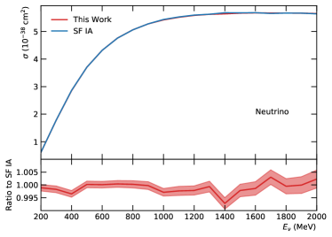
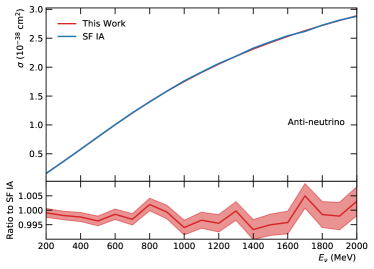
Figure 3: A comparison between our calculation and the SF IA based on Ref. Rocco et al. (2019a) for the total cross section for charged current scattering off a Carbon nucleus versus neutrino energy. On the left is the neutrino channel, while on the right is the anti-neutrino channel.

Additionally, the differential cross section is compared in Fig. 4 for the CC interaction at a fixed outgoing lepton angle of $30^{\circ}$ (left) and $70^{\circ}$ (right) for an incoming 1 GeV neutrino and anti-neutrino. Here we again see consistency between our method and that of Ref. Rocco et al. (2019a).

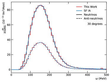
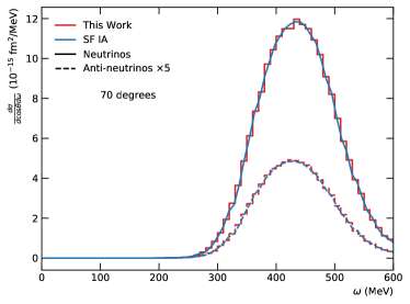
Figure 4: A comparison between our calculation and the SF IA based on Ref. Rocco et al. (2019a) for the double differential cross section for a 1 GeV neutrino on a Carbon target, with a fixed outgoing lepton angle of 30 degrees on the left and 70 degrees on the right.

VI.3 Neutrino Tridents

Figure 5: The two Feynman diagrams representing the neutrino trident cross section.

To demonstrate that this generator is not limited to $2\to 2$ process only and that it can handle interference terms, we consider the neutrino trident process $\nu_{\mu}\,^{12}{\rm C}\to\nu_{\mu}e^{+}e^{-}X$ with a fixed neutrino beam energy of 1 GeV, including both the $Z$ and photon interactions with the nucleon. Additionally, this process is an important background to understand for multiple lepton final state BSM explanations of the MiniBooNE excess. The Feynman diagrams for this process can be found in Fig. 5. In order to regulate the electron propagator pole, we set a minimum opening angle between the two electrons of $5^{\circ}$. In addition to this cut, we also require that the electrons have a minimum energy of 30 MeV, and have an angle from the neutrino beam axis greater than $10^{\circ}$. The electroweak parameters and form factors are identical to those used in the electron and neutrino scattering results section. With this setup, we obtain a total cross section of $3.973\times 10^{-14}\pm 2.764\times 10^{-17}$ nb, which is consistent with the results of Ref. Ballett et al. (2019c). In addition, we show the results for the electron pair opening angle, the leading electron energy, the sub-leading electron energy, and the invariant mass of the electron pair. The electron pair opening angle can be seen in Fig. 6, and is defined as the angle between the two electrons. This observable is important in understanding the ability of the next-generation experiments to observe this process for the first time based on their resolution for separating the two electrons from a single electron. The leading and sub-leading electron energy can be seen in Fig. 7. In comparing the leading and sub-leading energies, we see that one electron tends to be significantly softer than the other electron. Finally, the electron pair invariant mass can be seen in Fig. 8. This is an important observable to distinguish neutrino trident processes from BSM scenarios that have a pair of electrons in the final state, such as Ref. Bertuzzo et al. (2018b). In the case of Ref. Bertuzzo et al. (2018b), the $Z^{\prime}$ will create a bump in the invariant mass spectrum, which would be easily distinguishable from the standard neutrino trident prediction. We leave a detailed analysis of separating the standard neutrino trident from $Z^{\prime}$ models to a future work.

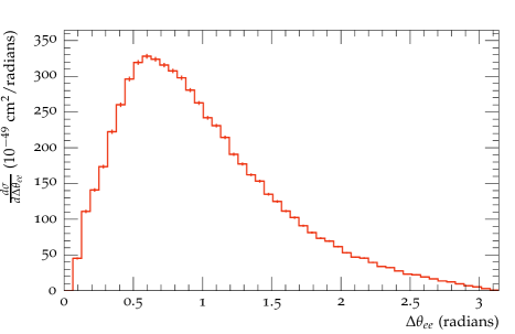
Figure 6: The opening angle between the two electrons in the neutrino trident process with an incoming neutrino beam of 1 GeV. A cut is placed on the minimum opening angle of $5^{\circ}$, and the electrons are required to have a minimum energy of 30 MeV.

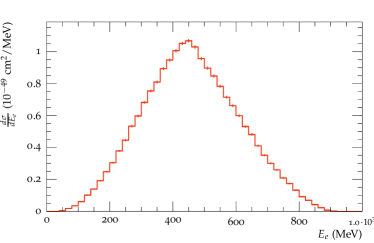
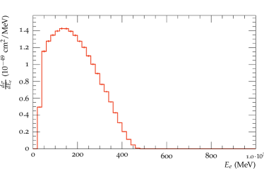
Figure 7: The leading (left) and sub-leading (right) energy for the outgoing electrons in the neutrino trident process with an incoming neutrino beam of 1 GeV. A cut is placed on the minimum opening angle between the electrons of $5^{\circ}$, and the electrons are required to have a minimum energy of 30 MeV.

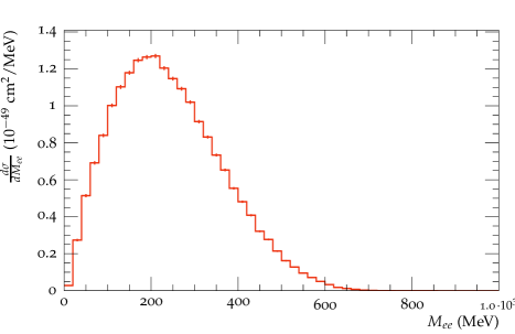
Figure 8: The invariant mass of the electron pair from the neutrino trident process with an incoming neutrino beam of 1 GeV. A cut is placed on the minimum opening angle between the electrons of $5^{\circ}$, and the electrons are required to have a minimum energy of 30 MeV.

VII Conclusions

We developed a novel event generation framework for the automated simulation of neutrino scattering at next-generation neutrino experiments. The framework takes inspiration from similar tools developed for the automatic simulation of events for the LHC community. The major complication that does not exist at the LHC is the handling of the nuclear physics effects, which we address by interfacing to a dedicated code for nuclear physics models in the quasielastic scattering region. Adding in the two-body currents, resonance production, shallow inelastic scattering, and deep inelastic scattering contributions is a logical extension of this work. This would require updating the handling of the initial states for the nuclear side, modifying the energy conserving delta function such that the phase space techniques described here can be applied, and implementing the additional nuclear effects. We leave this to a future work.

We demonstrate that we reproduce the expected results for the commonly studied processes of electron scattering and neutrino scattering off nuclei. Furthermore, we demonstrate the ability of the framework to compute processes beyond $2\to 2$ scattering by studying neutrino tridents. This process is important for multi-lepton final state explanations of the MiniBooNE excess. We show a variety of differential distributions demonstrating that this framework is capable of simulating full-differential events for subsequent analysis in the experimental simulation pipelines.

With the development of our new event generator, it becomes straightforward to study possible beyond Standard Model physics scenarios in a rigorous manner. Since the results obtained from the generator are fully differential in the many-body phase space and include the complete nuclear effects, our framework can assist the experiments in defining improved search strategies to separate various BSM scenarios from the Standard Model and from each other. We leave the details of this procedure to a future work.

The source code for our event generator will be provided upon request, and made public upon publication of this work.

VIII Acknowledgments

We thank Pedro Machado, William Jay, Alessandro Lovato, and Gil Paz for useful discussions and advice throughout the development of this tool. This manuscript has been authored by Fermi Research Alliance, LLC under Contract No. DE-AC02-07CH11359 with the U.S. Department of Energy, Office of Science, Office of High Energy Physics.

Appendix A Natively supported Lorentz structures

To exemplify the generality of our code, we list in this appendix the nontrivial expressions for the natively implemented Lorentz structures, not including those that correspond to simple contractions of external polarization vectors or spinors. The building blocks given here can be extended to nearly arbitrary interactions (also including higher-point functions) by means of the interface to FeynRules and UFO published in Ref. Höche et al. (2015).

$$\parbox{56.9055pt}{\begin{center} \fmfset{thick}{1.25thin} \fmfset{arrow_len}{2mm}\fmfset{curly_len}{1.5mm} \fmfset{wiggly_len}{1.5mm}\fmfset{decor_size}{2mm} \fmfset{dot_len}{1mm}\fmfset{dot_size}{2thick} \fmfset{dash_len}{1.5mm} \fmfgraph*(25,20) \fmftop{i,j} \fmfbottom{ij} \fmf{fermion}{v1,i} \fmf{photon}{j,v1} \fmf{fermion,tension=1.5}{v2,v1} \fmf{phantom,tension=5}{ij,v2} \fmfv{d.size=0,l.d=3.0,l.a=90,l=$\displaystyle\bar{u}$}{i} \fmfv{d.size=0,l.d=3.0,l.a=90,l=$\displaystyle j$}{j} \fmfv{d.shape=circle,d.size=3,l.a=0}{v2} \end{center}}=\bar{u}j^{\mu}\gamma_{\mu} =\left(0,0,\bar{u}_{0}j^{-}-\bar{u}_{1}j_{\perp},-\bar{u}_{0}j_{\perp}^{*}+\bar{u}_{1}j^{+}\right)\;,$$ (23)

$$\parbox{56.9055pt}{\begin{center} \fmfset{thick}{1.25thin} \fmfset{arrow_len}{2mm}\fmfset{curly_len}{1.5mm} \fmfset{wiggly_len}{1.5mm}\fmfset{decor_size}{2mm} \fmfset{dot_len}{1mm}\fmfset{dot_size}{2thick} \fmfset{dash_len}{1.5mm} \fmfgraph*(25,20) \fmftop{i,j} \fmfbottom{ij} \fmf{photon}{v1,i} \fmf{fermion}{j,v1} \fmf{fermion,tension=1.5}{v1,v2} \fmf{phantom,tension=5}{ij,v2} \fmfv{d.size=0,l.d=3.0,l.a=90,l=$\displaystyle j$}{i} \fmfv{d.size=0,l.d=3.0,l.a=90,l=$\displaystyle v$}{j} \fmfv{d.shape=circle,d.size=3,l.a=0}{v2} \end{center}}=j^{\mu}\gamma_{\mu}\frac{1-\gamma^{5}}{2}v =\left(\begin{array}[]{c}0\\ 0\\ j^{+}v_{0}+j_{\perp}^{*}v_{1}\\ j_{\perp}v_{0}+j^{-}v_{1}\end{array}\right)\;,$$ (28)

$$\parbox{56.9055pt}{\begin{center} \fmfset{thick}{1.25thin} \fmfset{arrow_len}{2mm}\fmfset{curly_len}{1.5mm} \fmfset{wiggly_len}{1.5mm}\fmfset{decor_size}{2mm} \fmfset{dot_len}{1mm}\fmfset{dot_size}{2thick} \fmfset{dash_len}{1.5mm} \fmfgraph*(25,20) \fmftop{i,j} \fmfbottom{ij} \fmf{fermion}{i,v1,j} \fmf{photon,tension=1.5}{v1,v2} \fmf{phantom,tension=5}{ij,v2} \fmfv{d.size=0,l.d=3.0,l.a=90,l=$\displaystyle\bar{u}$}{i} \fmfv{d.size=0,l.d=3.0,l.a=90,l=$\displaystyle v$}{j} \fmfv{d.shape=circle,d.size=3,l.a=0}{v2} \end{center}}=\bar{u}\gamma^{\mu}\frac{1-\gamma^{5}}{2}v=\left(\begin{array}[]{c}\bar{u}_{0}v_{2}+\bar{u}_{1}v_{3}\\ \bar{u}_{0}v_{3}+\bar{u}_{1}v_{2}\\ i\left(\bar{u}_{1}v_{2}-\bar{u}_{0}v_{3}\right)\\ \bar{u}_{0}v_{2}-\bar{u}_{1}v_{3}\end{array}\right)\;,$$ (33)

$$\parbox{56.9055pt}{\begin{center} \fmfset{thick}{1.25thin} \fmfset{arrow_len}{2mm}\fmfset{curly_len}{1.5mm} \fmfset{wiggly_len}{1.5mm}\fmfset{decor_size}{2mm} \fmfset{dot_len}{1mm}\fmfset{dot_size}{2thick} \fmfset{dash_len}{1.5mm} \fmfgraph*(25,20) \fmftop{i,j} \fmfbottom{ij} \fmf{fermion}{v1,i} \fmf{photon}{j,v1} \fmf{fermion,tension=1.5}{v2,v1} \fmf{phantom,tension=5}{ij,v2} \fmfv{d.size=0,l.d=3.0,l.a=90,l=$\displaystyle\bar{u}$}{i} \fmfv{d.size=0,l.d=3.0,l.a=90,l=$\displaystyle j$}{j} \fmfv{d.shape=circle,d.size=3,l.a=0}{v2} \end{center}}=\bar{u}j^{\mu}\gamma_{\mu}\frac{1+\gamma^{5}}{2} =\left(\bar{u}_{2}j^{+}+\bar{u}_{3}j_{\perp},\bar{u}_{2}j_{\perp}^{*}+\bar{u}_{3}j^{-},0,0\right)\;,$$ (34)

$$\parbox{56.9055pt}{\begin{center} \fmfset{thick}{1.25thin} \fmfset{arrow_len}{2mm}\fmfset{curly_len}{1.5mm} \fmfset{wiggly_len}{1.5mm}\fmfset{decor_size}{2mm} \fmfset{dot_len}{1mm}\fmfset{dot_size}{2thick} \fmfset{dash_len}{1.5mm} \fmfgraph*(25,20) \fmftop{i,j} \fmfbottom{ij} \fmf{photon}{v1,i} \fmf{fermion}{j,v1} \fmf{fermion,tension=1.5}{v1,v2} \fmf{phantom,tension=5}{ij,v2} \fmfv{d.size=0,l.d=3.0,l.a=90,l=$\displaystyle j$}{i} \fmfv{d.size=0,l.d=3.0,l.a=90,l=$\displaystyle v$}{j} \fmfv{d.shape=circle,d.size=3,l.a=0}{v2} \end{center}}=j^{\mu}\gamma_{\mu}\frac{1+\gamma^{5}}{2}v =\left(\begin{array}[]{c}j^{-}v_{2}-j_{\perp}^{*}v_{3}\\ -j_{\perp}v_{2}+j^{+}v_{3}\\ 0\\ 0\end{array}\right)\;,$$ (39)

$$\parbox{56.9055pt}{\begin{center} \fmfset{thick}{1.25thin} \fmfset{arrow_len}{2mm}\fmfset{curly_len}{1.5mm} \fmfset{wiggly_len}{1.5mm}\fmfset{decor_size}{2mm} \fmfset{dot_len}{1mm}\fmfset{dot_size}{2thick} \fmfset{dash_len}{1.5mm} \fmfgraph*(25,20) \fmftop{i,j} \fmfbottom{ij} \fmf{fermion}{i,v1,j} \fmf{photon,tension=1.5}{v1,v2} \fmf{phantom,tension=5}{ij,v2} \fmfv{d.size=0,l.d=3.0,l.a=90,l=$\displaystyle\bar{u}$}{i} \fmfv{d.size=0,l.d=3.0,l.a=90,l=$\displaystyle v$}{j} \fmfv{d.shape=circle,d.size=3,l.a=0}{v2} \end{center}}=\bar{u}\gamma^{\mu}\frac{1+\gamma^{5}}{2}v=\left(\begin{array}[]{c}\bar{u}_{2}v_{0}+\bar{u}_{3}v_{1}\\ -\bar{u}_{2}v_{1}-\bar{u}_{3}v_{0}\\ i\left(\bar{u}_{2}v_{1}-\bar{u}_{3}v_{0}\right)\\ -\bar{u}_{2}v_{0}+\bar{u}_{3}v_{1}\end{array}\right)\;,$$ (44)

$$\parbox{56.9055pt}{\begin{center} \fmfset{thick}{1.25thin} \fmfset{arrow_len}{2mm}\fmfset{curly_len}{1.5mm} \fmfset{wiggly_len}{1.5mm}\fmfset{decor_size}{2mm} \fmfset{dot_len}{1mm}\fmfset{dot_size}{2thick} \fmfset{dash_len}{1.5mm} \fmfgraph*(25,20) \fmftop{i,j} \fmfbottom{ij} \fmf{photon}{i,v1,j} \fmf{photon,tension=1.5}{v1,v2} \fmf{phantom,tension=5}{ij,v2} \fmfv{d.size=0,l.d=3.0,l.a=90,l=$\displaystyle j(p)$}{i} \fmfv{d.size=0,l.d=3.0,l.a=90,l=$\displaystyle j^{\prime}(q)$}{j} \fmfv{d.shape=circle,d.size=3,l.a=0}{v2} \end{center}}=\Gamma^{\mu\lambda\kappa}\left(p,q\right)j_{\lambda}j^{\prime}_{\kappa} =jj^{\prime}\left(p-q\right)^{\mu}+j^{\prime}\left(2q+p\right)j^{\mu}-j\left(2p+q\right)j^{\prime\mu}\;,$$ (45)

$$\parbox{56.9055pt}{\begin{center} \fmfset{thick}{1.25thin} \fmfset{arrow_len}{2mm}\fmfset{curly_len}{1.5mm} \fmfset{wiggly_len}{1.5mm}\fmfset{decor_size}{2mm} \fmfset{dot_len}{1mm}\fmfset{dot_size}{2thick} \fmfset{dash_len}{1.5mm} \fmfgraph*(25,20) \fmftop{i,j,k} \fmfbottom{ijk} \fmf{photon}{v1,i} \fmf{photon}{v1,j} \fmf{photon}{v1,k} \fmf{photon,tension=3}{v1,v2} \fmf{phantom,tension=5}{ijk,v2} \fmfv{d.size=0,l.d=3.0,l.a=90,l=$\displaystyle j$}{i} \fmfv{d.size=0,l.d=3.0,l.a=90,l=$\displaystyle j^{\prime}$}{j} \fmfv{d.size=0,l.d=3.0,l.a=90,l=$\displaystyle j^{\prime\prime}$}{k} \fmfv{d.shape=circle,d.size=3,l.a=0}{v2} \end{center}}=(2g^{\mu\nu}g^{\lambda\kappa}-g^{\mu\lambda}g^{\nu\kappa}-g^{\mu\kappa}g^{\nu\lambda})j_{\nu}j^{\prime}_{\kappa}j^{\prime\prime}_{\lambda} =2(j^{\prime}j^{\prime\prime})j^{\mu}-(jj^{\prime})j^{\prime\prime\mu}-(jj^{\prime\prime})j^{\prime\mu}\;,$$ (46)

References

- Abi et al. (2021) B. Abi et al. (DUNE), Eur. Phys. J. C 81, 322 (2021), arXiv:2008.12769 [hep-ex] .
- Abi et al. (2020) B. Abi et al. (DUNE), (2020), arXiv:2002.03005 [hep-ex] .
- Abe et al. (2018) K. Abe et al. (Hyper-Kamiokande), (2018), arXiv:1805.04163 [physics.ins-det] .
- Yano (2021) T. Yano (Hyper-Kamiokande), PoS ICRC2021, 1193 (2021).
- Aguilar et al. (2001) A. Aguilar et al. (LSND), Phys. Rev. D 64, 112007 (2001).
- Aguilar-Arevalo et al. (2007) A. A. Aguilar-Arevalo et al. (MiniBooNE), Phys. Rev. Lett. 98, 231801 (2007).
- Aguilar-Arevalo et al. (2009) A. A. Aguilar-Arevalo et al. (MiniBooNE), Phys. Rev. Lett. 102, 101802 (2009).
- Aguilar-Arevalo et al. (2010) A. A. Aguilar-Arevalo et al. (MiniBooNE), Phys. Rev. Lett. 105, 181801 (2010).
- Aguilar-Arevalo et al. (2013) A. A. Aguilar-Arevalo et al. (MiniBooNE), Phys. Rev. Lett. 110, 161801 (2013).
- Aguilar-Arevalo et al. (2018) A. A. Aguilar-Arevalo et al. (MiniBooNE), Phys. Rev. Lett. 121, 221801 (2018), arXiv:1805.12028 [hep-ex] .
- Aguilar-Arevalo et al. (2021) A. A. Aguilar-Arevalo et al. (MiniBooNE), Phys. Rev. D 103, 052002 (2021), arXiv:2006.16883 [hep-ex] .
- Gninenko (2009) S. Gninenko, Phys. Rev. Lett. 103, 241802 (2009), arXiv:0902.3802 [hep-ph] .
- McKeen and Pospelov (2010) D. McKeen and M. Pospelov, Phys. Rev. D 82, 113018 (2010), arXiv:1011.3046 [hep-ph] .
- Gninenko (2011) S. N. Gninenko, Phys. Rev. D 83, 015015 (2011), arXiv:1009.5536 [hep-ph] .
- Dib et al. (2011) C. Dib, J. C. Helo, S. Kovalenko, and I. Schmidt, Phys. Rev. D 84, 071301 (2011), arXiv:1105.4664 [hep-ph] .
- Gninenko (2012) S. Gninenko, Phys. Lett. B 710, 86 (2012), arXiv:1201.5194 [hep-ph] .
- Masip et al. (2013) M. Masip, P. Masjuan, and D. Meloni, JHEP 01, 106 (2013), arXiv:1210.1519 [hep-ph] .
- Ballett et al. (2017) P. Ballett, S. Pascoli, and M. Ross-Lonergan, JHEP 04, 102 (2017), arXiv:1610.08512 [hep-ph] .
- Magill et al. (2018) G. Magill, R. Plestid, M. Pospelov, and Y.-D. Tsai, Phys. Rev. D 98, 115015 (2018), arXiv:1803.03262 [hep-ph] .
- Fischer et al. (2020) O. Fischer, A. Hernández-Cabezudo, and T. Schwetz, Phys. Rev. D 101, 075045 (2020), arXiv:1909.09561 [hep-ph] .
- Bertuzzo et al. (2018a) E. Bertuzzo, S. Jana, P. A. N. Machado, and R. Zukanovich Funchal, (2018a), arXiv:1808.02500 [hep-ph] .
- Bertuzzo et al. (2018b) E. Bertuzzo, S. Jana, P. A. N. Machado, and R. Zukanovich Funchal, Phys. Rev. Lett. 121, 241801 (2018b), arXiv:1807.09877 [hep-ph] .
- Ballett et al. (2019a) P. Ballett, S. Pascoli, and M. Ross-Lonergan, Phys. Rev. D 99, 071701 (2019a), arXiv:1808.02915 [hep-ph] .
- Argüelles et al. (2019) C. A. Argüelles, M. Hostert, and Y.-D. Tsai, Phys. Rev. Lett. 123, 261801 (2019), arXiv:1812.08768 [hep-ph] .
- Ballett et al. (2019b) P. Ballett, M. Hostert, and S. Pascoli, Phys. Rev. D99, 091701 (2019b), arXiv:1903.07590 [hep-ph] .
- Ballett et al. (2020) P. Ballett, M. Hostert, and S. Pascoli, Phys. Rev. D 101, 115025 (2020), arXiv:1903.07589 [hep-ph] .
- Abdullahi et al. (2020) A. Abdullahi, M. Hostert, and S. Pascoli, (2020), arXiv:2007.11813 [hep-ph] .
- Abdallah et al. (2020a) W. Abdallah, R. Gandhi, and S. Roy, (2020a), arXiv:2010.06159 [hep-ph] .
- Abdallah et al. (2020b) W. Abdallah, R. Gandhi, and S. Roy, JHEP 12, 188 (2020b), arXiv:2006.01948 [hep-ph] .
- de Gouvêa et al. (2020) A. de Gouvêa, O. L. G. Peres, S. Prakash, and G. V. Stenico, JHEP 07, 141 (2020), arXiv:1911.01447 [hep-ph] .
- Dentler et al. (2020) M. Dentler, I. Esteban, J. Kopp, and P. Machado, Phys. Rev. D 101, 115013 (2020), arXiv:1911.01427 [hep-ph] .
- Chang et al. (2021) C.-H. V. Chang, C.-R. Chen, S.-Y. Ho, and S.-Y. Tseng, Phys. Rev. D 104, 015030 (2021), arXiv:2102.05012 [hep-ph] .
- (33) P. Abratenko (MicroBooNE), .
- Christensen and Duhr (2009) N. D. Christensen and C. Duhr, Comput. Phys. Commun. 180, 1614 (2009), arXiv:0806.4194 [hep-ph] .
- Alloul et al. (2014) A. Alloul, N. D. Christensen, C. Degrande, C. Duhr, and B. Fuks, Comput.Phys.Commun. 185, 2250 (2014), arXiv:1310.1921 [hep-ph] .
- Christensen et al. (2011) N. D. Christensen, P. de Aquino, C. Degrande, C. Duhr, B. Fuks, M. Herquet, F. Maltoni, and S. Schumann, Eur. Phys. J. C71, 1541 (2011), arXiv:0906.2474 [hep-ph] .
- Christensen et al. (2012) N. D. Christensen, C. Duhr, B. Fuks, J. Reuter, and C. Speckner, Eur. Phys. J. C 72, 1990 (2012), arXiv:1010.3251 [hep-ph] .
- Degrande et al. (2012) C. Degrande, C. Duhr, B. Fuks, D. Grellscheid, O. Mattelaer, and T. Reiter, Comput.Phys.Commun. 183, 1201 (2012), arXiv:1108.2040 [hep-ph] .
- Krauss et al. (2002) F. Krauss, R. Kuhn, and G. Soff, JHEP 02, 044 (2002), hep-ph/0109036 .
- Gleisberg and Höche (2008) T. Gleisberg and S. Höche, JHEP 12, 039 (2008), arXiv:0808.3674 [hep-ph] .
- Bähr et al. (2008) M. Bähr, S. Gieseke, M. A. Gigg, D. Grellscheid, K. Hamilton, O. Latunde-Dada, S. Plätzer, P. Richardson, M. H. Seymour, A. Sherstnev, and B. R. Webber, The European Physical Journal C 58, 639 (2008).
- Bellm et al. (2016) J. Bellm et al., Eur. Phys. J. C 76, 196 (2016), arXiv:1512.01178 [hep-ph] .
- Alwall et al. (2014) J. Alwall, R. Frederix, S. Frixione, V. Hirschi, F. Maltoni, O. Mattelaer, H.-S. Shao, T. Stelzer, P. Torrielli, M. Zaro, and et al., Journal of High Energy Physics 2014 (2014), 10.1007/jhep07(2014)079.
- Kilian et al. (2007) W. Kilian, T. Ohl, and J. Reuter, Eur. Phys. J. C71, 1742 (2007), arXiv:0708.4233 [hep-ph] .
- Sjöstrand et al. (2006) T. Sjöstrand, S. Mrenna, and P. Skands, JHEP 05, 026 (2006), hep-ph/0603175 .
- Sjöstrand et al. (2015) T. Sjöstrand, S. Ask, J. R. Christiansen, R. Corke, N. Desai, P. Ilten, S. Mrenna, S. Prestel, C. O. Rasmussen, and P. Z. Skands, Comput. Phys. Commun. 191, 159 (2015), arXiv:1410.3012 [hep-ph] .
- Gleisberg et al. (2009) T. Gleisberg, S. Höche, F. Krauss, M. Schönherr, S. Schumann, F. Siegert, and J. Winter, JHEP 02, 007 (2009), arXiv:0811.4622 [hep-ph] .
- Bothmann et al. (2019) E. Bothmann et al. (Sherpa), SciPost Phys. 7, 034 (2019), arXiv:1905.09127 [hep-ph] .
- Juszczak et al. (2006) C. Juszczak, J. A. Nowak, and J. T. Sobczyk, Nucl. Phys. B Proc. Suppl. 159, 211 (2006), arXiv:hep-ph/0512365 .
- Andreopoulos (2009) C. Andreopoulos (GENIE), Acta Phys. Polon. B 40, 2461 (2009).
- Hayato (2009) Y. Hayato, Acta Phys. Polon. B 40, 2477 (2009).
- Buss et al. (2012) O. Buss, T. Gaitanos, K. Gallmeister, H. van Hees, M. Kaskulov, O. Lalakulich, A. B. Larionov, T. Leitner, J. Weil, and U. Mosel, Phys. Rept. 512, 1 (2012), arXiv:1106.1344 [hep-ph] .
- Benhar et al. (2008) O. Benhar, D. day, and I. Sick, Rev. Mod. Phys. 80, 189 (2008), arXiv:nucl-ex/0603029 .
- Rocco et al. (2019a) N. Rocco, C. Barbieri, O. Benhar, A. De Pace, and A. Lovato, Phys. Rev. C 99, 025502 (2019a), arXiv:1810.07647 [nucl-th] .
- Dickhoff and Charity (2019) W. H. Dickhoff and R. J. Charity, Prog. Part. Nucl. Phys. 105, 252 (2019), arXiv:1811.03111 [nucl-th] .
- Dickhoff and Atkinson (2020) W. H. Dickhoff and M. C. Atkinson, J. Phys. Conf. Ser. 1643, 012082 (2020), arXiv:1909.13750 [nucl-th] .
- Barbieri and Hjorth-Jensen (2009) C. Barbieri and M. Hjorth-Jensen, Phys. Rev. C 79, 064313 (2009), arXiv:0902.3942 [nucl-th] .
- Benhar et al. (1994) O. Benhar, A. Fabrocini, S. Fantoni, and I. Sick, Nucl. Phys. A 579, 493 (1994).
- Sick et al. (1994) I. Sick, S. Fantoni, A. Fabrocini, and O. Benhar, Phys. Lett. B 323, 267 (1994).
- Rocco and Barbieri (2018) N. Rocco and C. Barbieri, Phys. Rev. C 98, 025501 (2018), arXiv:1803.00825 [nucl-th] .
- Andreoli et al. (2021) L. Andreoli, J. Carlson, A. Lovato, S. Pastore, N. Rocco, and R. B. Wiringa, (2021), arXiv:2108.10824 [nucl-th] .
- Ankowski et al. (2015) A. M. Ankowski, O. Benhar, and M. Sakuda, Phys. Rev. D 91, 033005 (2015), arXiv:1404.5687 [nucl-th] .
- Benhar et al. (1989) O. Benhar, A. Fabrocini, and S. Fantoni, Nucl. Phys. A 497, 423C (1989).
- Gleisberg et al. (2004) T. Gleisberg, S. Höche, F. Krauss, A. Schälicke, S. Schumann, and J. Winter, JHEP 02, 056 (2004), hep-ph/0311263 .
- Duhr et al. (2006) C. Duhr, S. Höche, and F. Maltoni, JHEP 08, 062 (2006), hep-ph/0607057 .
- Kanaki and Papadopoulos (2000) A. Kanaki and C. G. Papadopoulos, Comput. Phys. Commun. 132, 306 (2000), hep-ph/0002082 .
- Mangano et al. (2003) M. L. Mangano, M. Moretti, F. Piccinini, R. Pittau, and A. D. Polosa, JHEP 07, 001 (2003), hep-ph/0206293 .
- Höche et al. (2015) S. Höche, S. Kuttimalai, S. Schumann, and F. Siegert, Eur. Phys. J. C75, 135 (2015), arXiv:1412.6478 [hep-ph] .
- Krauss et al. (2017) F. Krauss, S. Kuttimalai, and T. Plehn, Phys. Rev. D95, 035024 (2017), arXiv:1611.00767 [hep-ph] .
- Hirschi et al. (2011) V. Hirschi, R. Frederix, S. Frixione, M. V. Garzelli, F. Maltoni, and R. Pittau, JHEP 05, 044 (2011), arXiv:1103.0621 [hep-ph] .
- Denner et al. (2018) A. Denner, J.-N. Lang, and S. Uccirati, Comput. Phys. Commun. 224, 346 (2018), arXiv:1711.07388 [hep-ph] .
- Buccioni et al. (2019) F. Buccioni, J.-N. Lang, J. M. Lindert, P. Maierhöfer, S. Pozzorini, H. Zhang, and M. F. Zoller, Eur. Phys. J. C 79, 866 (2019), arXiv:1907.13071 [hep-ph] .
- Byckling and Kajantie (1969) E. Byckling and K. Kajantie, Nucl. Phys. B9, 568 (1969).
- Kleiss and Pittau (1994) R. Kleiss and R. Pittau, Comput. Phys. Commun. 83, 141 (1994), arXiv:hep-ph/9405257 [hep-ph] .
- Lepage (1980) G. P. Lepage, (1980), cLNS-80/447.
- Adamson et al. (2016) P. Adamson et al., Nucl. Instrum. Meth. A 806, 279 (2016), arXiv:1507.06690 [physics.acc-ph] .
- (77) F. James, CERN-68-15.
- Lepage (1978) G. P. Lepage, J. Comput. Phys. 27, 192 (1978).
- Bothmann et al. (2020) E. Bothmann, T. Janßen, M. Knobbe, T. Schmale, and S. Schumann, SciPost Phys. 8, 069 (2020), arXiv:2001.05478 [hep-ph] .
- Gao et al. (2020) C. Gao, S. Höche, J. Isaacson, C. Krause, and H. Schulz, Phys. Rev. D 101, 076002 (2020), arXiv:2001.10028 [hep-ph] .
- Kelly (2004) J. J. Kelly, Phys. Rev. C 70, 068202 (2004).
- Meyer et al. (2016) A. S. Meyer, M. Betancourt, R. Gran, and R. J. Hill, Phys. Rev. D 93, 113015 (2016), arXiv:1603.03048 [hep-ph] .
- Rocco et al. (2019b) N. Rocco, S. X. Nakamura, T. S. H. Lee, and A. Lovato, Phys. Rev. C 100, 045503 (2019b), arXiv:1907.01093 [nucl-th] .
- Sealock et al. (1989) R. M. Sealock et al., Phys. Rev. Lett. 62, 1350 (1989).
- Ballett et al. (2019c) P. Ballett, M. Hostert, S. Pascoli, Y. F. Perez-Gonzalez, Z. Tabrizi, and R. Zukanovich Funchal, JHEP 01, 119 (2019c), arXiv:1807.10973 [hep-ph] .