Communication-Efficient ADMM-based Federated Learning

Abstract: Federated learning has shown its advances over the last few years but is facing many challenges, such as how algorithms save communication resources, how they reduce computational costs, and whether they converge. To address these issues, this paper proposes exact and inexact ADMM-based federated learning. They are not only communication-efficient but also converge linearly under very mild conditions, such as convexity-free and irrelevance to data distributions. Moreover, the inexact version has low computational complexity, thereby alleviating the computational burdens significantly.

Keywords: ADMM-based federated learning, efficient communications, low computational costs, global convergence with linear rate

1 Introduction

Federated learning, as an effective machine learning technique, gains popularity in recent years due to its ability to deal with various issues like data privacy, data security, and data access to heterogeneous data. Typical applications include vehicular communications [1, 2, 3, 4], digital health [5], and smart manufacturing [6], just to name a few. The earliest work for federated learning can be traced back to [7] in 2015 and [8] in 2016. It is still undergoing development and also facing many challenges. For example, how do algorithms save the communication resources during the learning process? What is their computational and convergence performance? We refer to some nice surveys [9, 10, 11] for more open questions.

1.1 Related work

(a) Saving communication resources. In distributed learning, local clients and a central server communicate frequently, which sometimes is relatively inefficient. For example, if the updated parameters from some local clients are negligible, then their impact on the global aggregation (or averaging) by the central server can be ignored. On the other hand, even though the updated parameters from some local clients are desirable, the channel conditions might be poor and thus more communication resources (e.g., transmission power and bandwidth) are required as a remedy. Therefore, saving communications resources which can be fulfilled by skipping or reducing unnecessary communication rounds tends to be inevitable in practical.

Motivated by this, there is an impressive body of work on developing algorithms that aims to reduce the communication rounds. The stochastic gradient descent (SGD) is one of the most extensively used schemes. It executes global aggregation in a periodic fashion so as to reduce the communication rounds [12, 13, 14, 15, 16, 17]. However, to establish the convergence theory, the family of SGD frequently assumes the data from local clients to be identically and independently distributed (i.i.d.), which is apparently unrealistic for federated learning settings where data distributions are heterogeneous.

A separated line of research investigates algorithms that make assumptions on the objective functions themselves, and hence they are irrelevant to the distributions of the involved data, such as the distributed gradient descent algorithm [18] for the edge computing in wireless communication, lazily aggregated gradient algorithm [19] for centralized learning, lazy and approximate dual gradients algorithm [20] for decentralized learning, and federated (iterative) hard thresholding algorithm [21]. Despite no assumptions on the data distributions, strong conditions are often imposed on the objective functions of the learning optimization problem, including (gradient) Lipschitz continuity, strong smoothness, convexity, or strong convexity.

(b) ADMM-based learning. Over the last few decades, the alternating direction method of multipliers (ADMM) has shown its advances both in theoretical and numerical aspects, with extensive applications into various disciplinarians. Fairly recently, there is a success of implementation ADMM into distributed learning [22, 23, 24, 25, 26, 27, 28, 29]. When it comes to federated learning settings, a robust ADMM-based decentralized federated learning has been proposed in [30] to mitigate the influence of some falsified data. Very lately, inexact ADMM has drawn some attention in federated learning, thanks to its ability to alleviate computational burdens. For instance, an inexact ADMM-based federated meta-learning algorithm has been cast in [31] for fast and continual edge learning and a differential private inexact ADMM-based federated learning algorithm has been designed in [32] to accelerate the computation and protect data privacy. Again, we shall emphasize that these algorithms have been provably convergent but still required some aforementioned restrictive assumptions.

1.2 Our contributions

In conventional federated learning, at every step, all local clients update their parameters in parallel and then send them to the central server for aggregation. When ADMM is applied into federated learning, it can be viewed as a scene where the local clients update not only their parameters but also the dual parameters of the target optimization problem, followed by the global aggregation from the central server using both parameters. In this regard, the scheme of the conventional federated learning can be deemed as a special case of ADMM. As a by-product of this paper, we reveal the relationship between federated learning and linearised inexact ADMM-based federated learning. Their frameworks are presented in Figure 1, from which one can see that the former can be deemed as a special case of the latter.

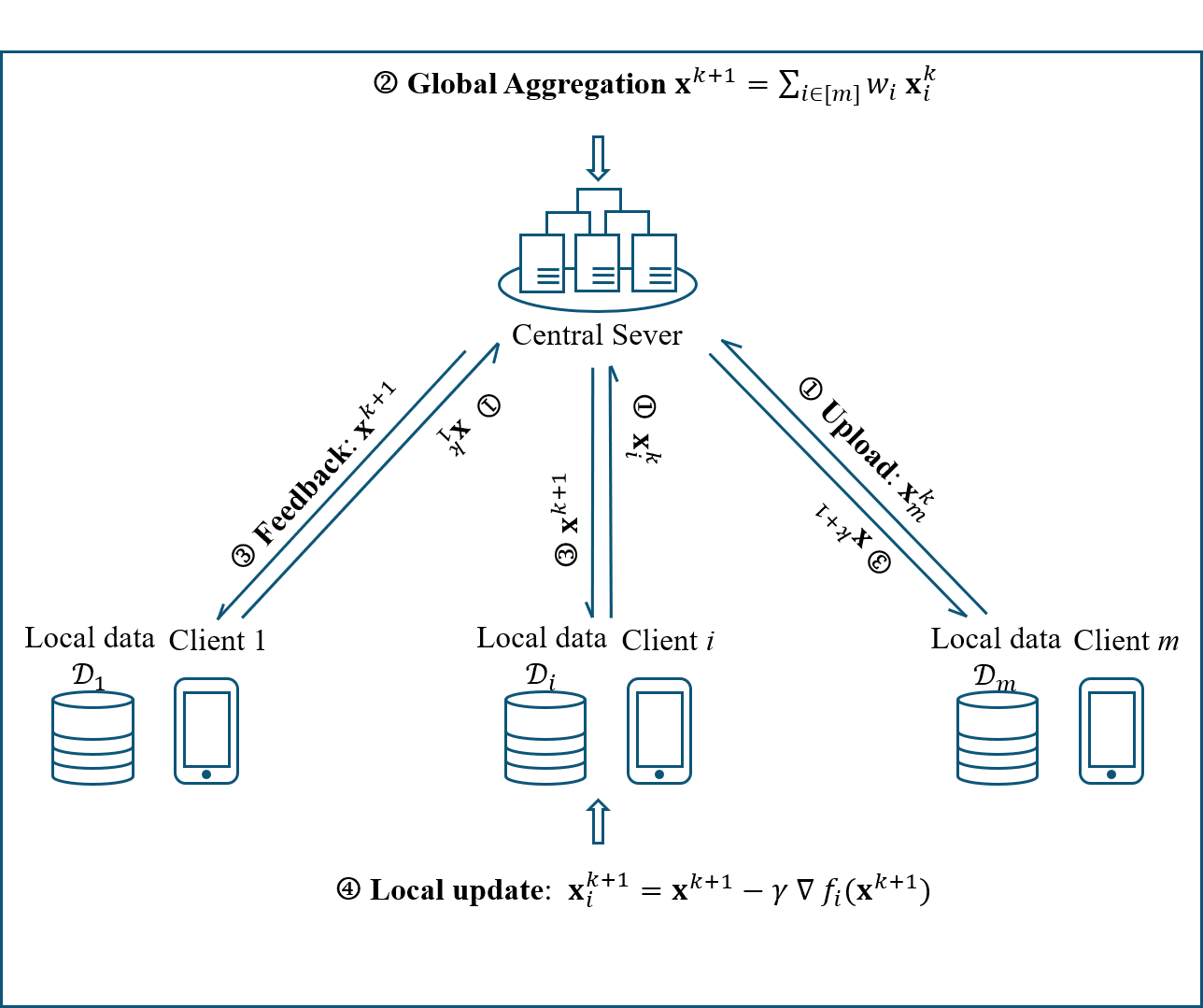
(a) Federated learning.

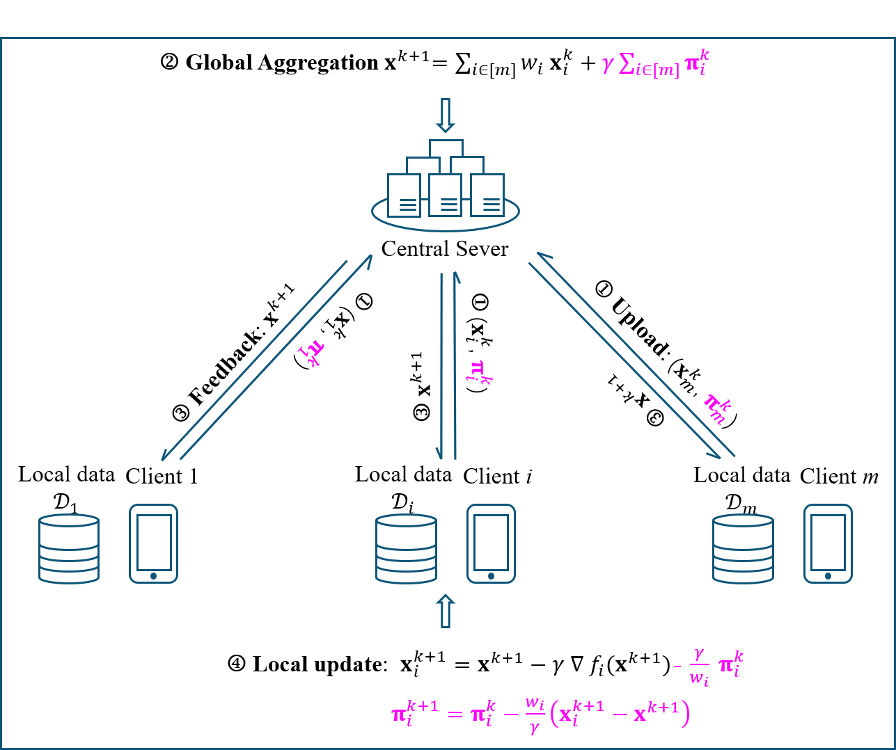
(b) Linearised inexact ADMM-based federated learning.

Figure 1: Algorithm 1 v.s. Algorithm 4.

The main contribution of this paper is developing two ADMM-based federated learning algorithms to save communication resources, reduce computational burdens, and converge under relatively weak assumptions.

I) Based on the framework of ADMM, we design a communication-efficient ADMM (CEADMM) algorithm and an inexact ADMM (ICEADMM) algorithm that reduce the communication rounds between the local clients and the central server. Precisely, between two rounds of communications, there are $k_{0}$ iterations allowing for local clients to update their parameters. The numerical experiments demonstrate that the larger $k_{0}$, the fewer communication rounds required to converge, as shown in Figures 5(b) or 5(e). This hints that setting a proper larger $k_{0}$ would save communication resources greatly.

II) To alleviate the computational burdens, ICEADMM is also capable of cutting down the computational costs, thereby accelerating the entire learning process dramatically, as shown in Figures 4(c) and 4(f). Nevertheless, the established theory and empirical numerical experiments show that ICEADMM does not compromise any accuracy.

III) Both algorithms converge to a stationary point (see Definition 2.1) of the learning optimization problem in (2.7) with a linear rate $O(k_{0}/k)$ only under two mild conditions: gradient Lipschitz continuity (also known for the L-smoothness in many publications) and the boundedness of a level set, as in Theorems 3.2 and 3.3, where $k$ is the iteration number and $k_{0}$ is the number of the gap between two rounds of communications. These conditions are convexity-free and independent of distributions of the data. Hence, they are weaker than those used to establish convergence for the current distributed and federated learning algorithms. If we further assume the convexity, then both algorithms can achieve the optimal parameters, as shown in Corollary 3.1.

1.3 Organization and notation

This paper is organized as follows. In the next section, we introduce federated learning and the framework of ADMM. In Section 3, we design the communication-efficient ADMM (CEADMM), followed by the establishment of its global convergence and the complexity analysis. Then similar results are achieved for the inexact communication-efficient ADMM (ICEADMM) in Section 4. In Section 5, we conduct some numerical experiments to demonstrate the performance of two algorithms and testify our established theorems. Concluding remarks are given in the last section.

We end this section with summarizing the notation that will be employed throughout this paper. We use plain, bold, and capital letters to present scalars, vectors, and matrices, respectively, e.g., $\gamma$ and $\sigma$ are scalars, $\mathbf{x},\mathbf{x}_{i}$ and $\mathbf{x}_{i}^{k}$ are vectors, $X$ and $X^{k}$ are matrices. Let $\lfloor t\rfloor$ represent the smallest integer that is no greater than $t$ and $[m]:=\{1,2,\ldots,m\}$ with ‘$:=$’ meaning define. In this paper, $\mathbb{R}^{n}$ denotes the $n$-dimensional Euclidean space equipped with the inner product $\langle\cdot,\cdot\rangle$ defined by $\langle\mathbf{x},\mathbf{y}\rangle:=\sum_{i}x_{i}y_{i}$. Let $\|\cdot\|$ be the Euclidean norm, namely, $\|\mathbf{x}\|^{2}=\langle\mathbf{x},\mathbf{x}\rangle$ and $\|\cdot\|_{H}$ be the weighted norm defined by $\|\mathbf{x}\|_{H}^{2}:=\langle H\mathbf{x},\mathbf{x}\rangle$. Write the identity matrix as $I$ and a positive semidefinite matrix $A$ as $A\succeq 0$. In particular, $A\succeq B$ represents $A-B\succeq 0$. A function, $f$, is said to be gradient Lipschitz continuous with a constant $r>0$ if

$$\|\nabla f(\mathbf{x})-\nabla f(\mathbf{z})\|\leq r\|\mathbf{x}-\mathbf{z}\|.$$ (1.1)

for any $\mathbf{x}$ and $\mathbf{z}$, where $\nabla f(\mathbf{x})$ represents the gradient of $f$ with respect to $\mathbf{x}$.

2 Federated Learning and ADMM

Suppose we have $m$ local clients/edge nodes with datasets $\{\mathcal{D}_{i}\}_{i\in[m]}$ as shown in Figure 1(b). Each client has the total loss $f_{i}(\mathbf{x}):=\sum_{{\boldsymbol{\theta}}\in\mathcal{D}_{i}}\ell_{i}(\mathbf{x};{\boldsymbol{\theta}})$, where $\ell_{i}(\cdot;{\boldsymbol{\theta}}):\mathbb{R}^{n}\mapsto\mathbb{R}$ is a continuous loss function and bounded from below, and $\mathbf{x}\in\mathbb{R}^{n}$ is the parameter to be learned. Below are two examples that will be used for our numerical experiments.

Example 2.1 (Least square loss).

Suppose the $i$th client has data $\mathcal{D}_{i}=\{(\mathbf{a}^{i}_{1},b^{i}_{1}),\ldots,(\mathbf{a}^{i}_{d_{i}},b^{i}_{d_{i}})\}$, where $\mathbf{a}^{i}_{j}\in\mathbb{R}^{n}$, $b^{i}_{j}\in\mathbb{R}$, and $d_{i}$ is the cardinality of $\mathcal{D}_{i}$. Let ${\boldsymbol{\theta}}:=(\mathbf{a},b)$, then the least square loss is defined by

$$\begin{array}[]{llll}f_{i}(\mathbf{x})&=&\sum_{j=1}^{d_{i}}\frac{1}{2}(\langle\mathbf{a}^{i}_{j},\mathbf{x}\rangle-b^{i}_{j})^{2}.\end{array}$$ (2.2)

Example 2.2 ($\ell_{2}$ norm regularized logistic loss).

Similarly, the $i$th client has data $\mathcal{D}_{i}$ but with $b^{i}_{j}\in\{0,1\}$. The $\ell_{2}$ norm regularized logistic loss is given by

$$\begin{array}[]{llll}f_{i}(\mathbf{x})&=&\sum_{j=1}^{d_{i}}[\ln(1+e^{\langle\mathbf{a}^{i}_{j},\mathbf{x}\rangle})-b^{i}_{j}\langle\mathbf{a}^{i}_{j},\mathbf{x}\rangle+\frac{\mu}{2d_{i}}\|\mathbf{x}\|^{2}],\end{array}$$ (2.4)

where $\mu>0$ is a penalty parameter.

The overall loss function can be defined by

$$\begin{array}[]{lll}f(\mathbf{x}):=\sum_{i=1}^{m}w_{i}f_{i}(\mathbf{x}),\end{array}$$

where $w_{i},i\in[m]$ are positive weights that satisfy $\sum_{i=1}^{m}w_{i}=1.$ Particular choices for such weights are $w_{i}=d_{i}/d$ with $d:=\sum_{i=1}^{m}d_{i}$. Federated learning aims to learn a best parameter $\mathbf{x}^{*}$ at the central server that minimizes the overall loss function, $f$, namely,

$$\begin{array}[]{lll}\mathbf{x}^{*}:={\rm argmin}_{\mathbf{x}\in\mathbb{R}^{n}}~{}f(\mathbf{x}).\end{array}$$ (2.7)

Since $f_{i}$ is bounded from below, we have

$$\begin{array}[]{lll}f^{*}:=f(\mathbf{x}^{*})>-\infty.\end{array}$$ (2.9)

By introducing auxiliary variables, $\mathbf{x}_{i}=\mathbf{x}$, problem (2.7) can be rewritten as

$$\begin{array}[]{lll}\underset{\mathbf{x},\mathbf{x}_{1},\ldots,\mathbf{x}_{m}\in\mathbb{R}^{n}}{\min}~{}~{}\sum_{i=1}^{m}w_{i}f_{i}(\mathbf{x}_{i}),~{}~{}{\rm s.t.}~{}~{}\mathbf{x}_{i}=\mathbf{x},~{}i\in[m].\end{array}$$ (2.11)

Throughout the paper, we shall place our interest on the above optimization problem. For simplicity, we also denote

$$\begin{array}[]{lll}F(X):=\sum_{i=1}^{m}w_{i}f_{i}(\mathbf{x}_{i}),\qquad{\rm where}\qquad X:=(\mathbf{x}_{1},\mathbf{x}_{2},\ldots,\mathbf{x}_{m}).\end{array}$$ (2.13)

It is easy to see that $f(\mathbf{x})=F(X)$ if $X=(\mathbf{x},\mathbf{x},\ldots,\mathbf{x})$.

2.1 Conventional federated learning

The conventional federated learning can be summarized as Algorithm 1.

Initialize $\mathbf{x}_{i}^{0}=\mathbf{x}^{0},i\in[m]$, a step size $\gamma>0$. Set $k\Leftarrow 0$.

for $k=0,1,2,\ldots$ do

      

      Weights upload: Each client sends the parameter $\mathbf{x}^{k}_{i}$ to the central server.

      Global aggregation: The central server calculates the average parameter $\mathbf{x}^{k+1}$ by

$$\begin{array}[]{lll}\mathbf{x}^{k+1}=\sum_{i=1}^{m}{w_{i}\mathbf{x}^{k}_{i}}.\end{array}$$ (2.15)

      Weights feedback: The central server broadcasts the parameter $\mathbf{x}^{k+1}$ to every local client.

      for $i=1,2,\ldots,m$ do

            Local update: Each client updates its parameter locally and in parallel by

$$\begin{array}[]{lll}\mathbf{x}^{k+1}_{i}=\mathbf{x}^{k+1}-\gamma\nabla f_{i}(\mathbf{x}^{k+1}).\end{array}$$ (2.17)

       end for

      

end for

Algorithm 1 Federated Learning

Since we initialize $\mathbf{x}_{i}^{0}=\mathbf{x}^{0},i\in[m]$ and $\sum_{i=1}^{m}w_{i}=1$, the first step has $\mathbf{x}^{1}=\sum_{i=1}^{m}{w_{i}\mathbf{x}^{0}_{i}}=\mathbf{x}^{0}$. Therefore,

$$\begin{array}[]{lll}\mathbf{x}^{1}_{i}=\mathbf{x}^{1}-\gamma\nabla f_{i}(\mathbf{x}^{1})=\mathbf{x}^{0}-\gamma\ \nabla f_{i}(\mathbf{x}^{0})=\mathbf{x}^{0}_{i}-\gamma\nabla f_{i}(\mathbf{x}^{0}_{i}).\end{array}$$ (2.19)

So the framework of Algorithm 1 is same as the standard one where the first step does the local update in (2.19), followed by the global aggregation. We prefer the framework of Algorithm 1 because it has a clearer and closer link to the framework of ADMM introduced in the sequel.

2.2 ADMM

We first briefly introduce some backgrounds of the alternating direction method of multipliers (ADMM). For more details, one can refer to the earliest work [33] and a nice book [22]. Suppose we are given an optimization problem,

$$\begin{array}[]{cll}\min\limits_{\mathbf{x}\in\mathbb{R}^{n},\mathbf{z}\in\mathbb{R}^{q}}~{}~{}f(\mathbf{x})+g(\mathbf{z}),\qquad{\rm s.t.}~{}~{}A\mathbf{x}+B\mathbf{z}=\mathbf{b},\end{array}$$ (2.21)

where $A\in\mathbb{R}^{p\times n}$, $B\in\mathbb{R}^{p\times q}$, and $\mathbf{b}\in\mathbb{R}^{p}$. To implement ADMM, we need the so-called augmented Lagrange function of problem (2.21), which is defined by

$$\begin{array}[]{lll}\mathcal{L}(\mathbf{x},\mathbf{z},{\boldsymbol{\pi}}):=f(\mathbf{x})+g(\mathbf{z})+\langle A\mathbf{x}+B\mathbf{z}-\mathbf{b},{\boldsymbol{\pi}}\rangle+\frac{\sigma}{2}\|A\mathbf{x}+B\mathbf{z}-\mathbf{b}\|^{2},\end{array}$$ (2.23)

where ${\boldsymbol{\pi}}$ is known for the Lagrange multiplier and $\sigma>0$. Based on the augmented Lagrange function, ADMM executes the following steps for a given starting point $(\mathbf{x}^{0},\mathbf{z}^{0},{\boldsymbol{\pi}}^{0})$ and any $k\geq 0$,

$$\begin{array}[]{llll}\mathbf{x}^{k+1}&=&{\rm argmin}_{\mathbf{x}\in\mathbb{R}^{n}}~{}\mathcal{L}(\mathbf{x},\mathbf{z}^{k},{\boldsymbol{\pi}}^{k}),\\ \mathbf{z}^{k+1}&=&{\rm argmin}_{\mathbf{z}\in\mathbb{R}^{q}}~{}\mathcal{L}(\mathbf{x}^{k+1},\mathbf{z},{\boldsymbol{\pi}}^{k}),\\ {\boldsymbol{\pi}}^{k+1}&=&{\boldsymbol{\pi}}^{k}+\sigma(A\mathbf{x}^{k+1}+B\mathbf{z}^{k+1}-\mathbf{b}).\end{array}$$ (2.27)

Therefore, to implement ADMM for our problem in (2.11), the corresponding augmented Lagrange function can be defined by,

$$\begin{array}[]{lll}\mathcal{L}(\mathbf{x},X,\Pi):=\sum_{i=1}^{m}L(\mathbf{x},\mathbf{x}_{i},{\boldsymbol{\pi}}_{i}),\end{array}$$ (2.29)

where $X:=(\mathbf{x}_{1},\mathbf{x}_{2},\ldots,\mathbf{x}_{m}),~{}\Pi:=({\boldsymbol{\pi}}_{1},{\boldsymbol{\pi}}_{2},\ldots,{\boldsymbol{\pi}}_{m})$, and $L(\mathbf{x},\mathbf{x}_{i},{\boldsymbol{\pi}}_{i})$ is

$$\begin{array}[]{lll}L(\mathbf{x},\mathbf{x}_{i},{\boldsymbol{\pi}}_{i}):=w_{i}f_{i}(\mathbf{x}_{i})+\langle\mathbf{x}_{i}-\mathbf{x},{\boldsymbol{\pi}}_{i}\rangle+\frac{\sigma_{i}}{2}\|\mathbf{x}_{i}-\mathbf{x}\|^{2}.\end{array}$$ (2.31)

Here, ${\boldsymbol{\pi}}_{i}\in\mathbb{R}^{n},i\in[m]$ are the Lagrange multipliers and $\sigma_{i}>0,i\in[m]$. Similar to (2.27), we have the framework of ADMM for problem (2.11). That is, for an initialized point $(\mathbf{x}^{0},X^{0},\Pi^{0})$ and any $k\geq 0$, perform the following updates iteratively,

$$\begin{array}[]{llll}\mathbf{x}^{k+1}&=&{\rm argmin}_{\mathbf{x}\in\mathbb{R}^{n}}~{}\mathcal{L}(\mathbf{x},X^{k},\Pi^{k}),\\ \mathbf{x}^{k+1}_{i}&=&{\rm argmin}_{\mathbf{x}_{i}\in\mathbb{R}^{n}}~{}L(\mathbf{x}^{k+1},\mathbf{x}_{i},{\boldsymbol{\pi}}_{i}^{k}),{}{}&i\in[m],\\ {\boldsymbol{\pi}}^{k+1}_{i}&=&{\boldsymbol{\pi}}_{i}^{k}+\sigma_{i}(\mathbf{x}_{i}^{k+1}-\mathbf{x}^{k+1}),{}{}&i\in[m].\end{array}$$ (2.35)

Initialize $\mathbf{x}_{i}^{0},{\boldsymbol{\pi}}_{i}^{0},\sigma_{i}>0,i\in[m]$. Set $k\Leftarrow 0$.

for $k=0,1,2,\ldots$ do

      

      Weights upload: Each client sends the parameters $\mathbf{x}^{k}_{i}$ and ${\boldsymbol{\pi}}_{i}^{k}$ to the central server.

      Global aggregation: The central server calculates the average parameter $\mathbf{x}^{k+1}$ by

$$\begin{array}[]{llll}\mathbf{x}^{k+1}&=&{\rm argmin}_{\mathbf{x}}~{}\mathcal{L}(\mathbf{x},X^{k},\Pi^{k}).\end{array}$$ (2.37)

Weights feedback: The central server broadcasts the parameter $\mathbf{x}^{k+1}$ to every local client.

      for $i=1,2,\ldots,m$ do

             Local update: Each client updates its parameters locally and in parallel by

$$\begin{array}[]{llll}\mathbf{x}^{k+1}_{i}&=&{\rm argmin}_{\mathbf{x}_{i}}~{}L(\mathbf{y}^{k+1},\mathbf{x}_{i},{\boldsymbol{\pi}}_{i}^{k}),{}{}{}{}\end{array}$$

$$\begin{array}[]{llll}{\boldsymbol{\pi}}^{k+1}_{i}&=&{\boldsymbol{\pi}}_{i}^{k}+\sigma_{i}(\mathbf{x}_{i}^{k+1}-\mathbf{y}^{k+1}).\end{array}$$

       end for

      

end for

Algorithm 2 ADMM-based federated learning

Integrating the standard ADMM into federated learning, we derive the algorithmic framework presented in Algorithm 2, where subproblem (2.37) can be derived by

$$\begin{array}[]{llll}\mathbf{x}^{k+1}={\rm argmin}_{\mathbf{x}}~{}\mathcal{L}(\mathbf{x},X^{k},\Pi^{k})=\sum_{i=1}^{m}\frac{{\sigma_{i}}\mathbf{x}^{k}_{i}}{\sigma}+\sum_{i=1}^{m}\frac{{\boldsymbol{\pi}}_{i}^{k}}{\sigma},\end{array}$$ (2.41)

with

$$\begin{array}[]{lll}\sigma:=\sum_{i=1}^{m}\sigma_{i}.\end{array}$$ (2.43)

It is noted that in traditional federated learning, as shown in (2.15), the central server usually calculates the parameter by using the averaged value of all local parameters, $\mathbf{x}_{i}^{k}$. Besides that, ADMM also exploits parameters ${\boldsymbol{\pi}}_{i}^{k}$ from the dual problem, see (2.41). If we set $\sigma_{i}=w_{i}/\gamma$ for all $i\in[m]$ and a given step size $\gamma$, then (2.41) turns to

$$\begin{array}[]{lll}\mathbf{x}^{k+1}=\sum_{i=1}^{m}w_{i}\mathbf{x}^{k}_{i}+{\gamma}\sum_{i=1}^{m}{\boldsymbol{\pi}}_{i}^{k}.\end{array}$$ (2.45)

It is very similar to (2.15) but with an additional term involving the dual parameter, ${\boldsymbol{\pi}}_{i}^{k}$.

2.3 Stationary points

To end this section, we present the optimality conditions of problems (2.11) and (2.7).

Definition 2.1.

A point $(\mathbf{x}^{*},X^{*},\Pi^{*})$ is a stationary point of problem (2.11) if it satisfies

$$\left\{\begin{array}[]{rcll}w_{i}\nabla f_{i}(\mathbf{x}_{i}^{*})+{\boldsymbol{\pi}}_{i}^{*}&=&0,{}{}&i\in[m],\\ \mathbf{x}_{i}^{*}-\mathbf{x}^{*}&=&0,&i\in[m],\\ \sum_{i=1}^{m}{\boldsymbol{\pi}}_{i}^{*}&=&0.\end{array}\right.$$ (2.49)

A point $\mathbf{x}^{*}$ is a stationary point of problem (2.7) if it satisfies

$$\begin{array}[]{llll}\nabla f(\mathbf{x}^{*})=0.\end{array}$$ (2.51)

It is not difficult to prove that any locally optimal solution to problem (2.11) (resp. (2.7)) must satisfy (2.49) (resp. (2.51)). If $f_{i}$ is convex for every $i\in[m]$, then a point is a globally optimal solution to problem (2.11) (resp.(2.7)) if and only if it satisfies condition (2.49) (resp. (2.51)). Moreover, it is easy to see that a stationary point $(\mathbf{x}^{*},X^{*},\Pi^{*})$ of problem (2.11) indicates

$$\begin{array}[]{llll}\nabla f(\mathbf{x}^{*})=\sum_{i=1}^{m}w_{i}\nabla f_{i}(\mathbf{x}^{*})=\sum_{i=1}^{m}w_{i}\nabla f_{i}(\mathbf{x}^{*}_{i})=0.\end{array}$$ (2.53)

That is, $\mathbf{x}^{*}$ is also a stationary point of problem (2.7).

3 Communication-Efficient ADMM

The framework of ADMM in (2.35) repeats the global aggregation and local update in every step. In federated learning (see Algorithm 2), this manifests that local clients and the central server have to communicate in every step. That is, the central server broadcasts to weight $\mathbf{x}^{k+1}$ all local clients, and each client uploads their weights $\mathbf{x}^{k+1}_{i}$ and ${\boldsymbol{\pi}}^{k+1}_{i}$ to the central server afterwards. However, frequent communications would come at a huge price, such as extremely long learning time and large amounts of resources, which should be avoided in reality.

Initialize $\mathbf{x}_{i}^{0},{\boldsymbol{\pi}}_{i}^{0},\sigma_{i}>0,i\in[m]$, an integer $k_{0}>0$. Set $k\Leftarrow 0$.

for $k=0,1,2,\ldots$ do

      

      if $k\in\mathcal{K}:=\{0,k_{0},2k_{0},3k_{0},\ldots\}$ then

             Weights upload: Each client sends its parameters $\mathbf{x}^{k}_{i}$ and ${\boldsymbol{\pi}}_{i}^{k}$ to the central server.

            Global aggregation: The central server calculates the average parameter $\mathbf{x}^{k+1}$ by

$$\begin{array}[]{llll}\mathbf{x}^{k+1}=\sum_{i=1}^{m}\frac{{\sigma_{i}}\mathbf{x}^{k}_{i}}{\sigma}+\sum_{i=1}^{m}\frac{{\boldsymbol{\pi}}_{i}^{k}}{\sigma}.\end{array}$$ (3.2)

Weights feedback: The central server broadcasts the parameter $\mathbf{x}^{k+1}$ to every client.

       end if

      for $i=1,2,\ldots,m$ do

             Local update: By letting

$$\mathbf{y}^{k+1}:=\mathbf{x}^{\tau_{k}+1},\qquad{\rm where}~{}~{}\tau_{k}:=\lfloor k/k_{0}\rfloor k_{0},$$

each client update its parameters locally and in parallel via solving

$$\begin{array}[]{llll}\mathbf{x}^{k+1}_{i}&=&{\rm argmin}_{\mathbf{x}_{i}}~{}w_{i}f_{i}(\mathbf{x}_{i})+\langle\mathbf{x}_{i}-\mathbf{y}^{k+1},{\boldsymbol{\pi}}_{i}^{k}\rangle+\frac{\sigma_{i}}{2}\|\mathbf{x}_{i}-\mathbf{y}^{k+1}\|^{2},\end{array}$$ (3.4)

$$\begin{array}[]{llll}{\boldsymbol{\pi}}^{k+1}_{i}&=&{\boldsymbol{\pi}}_{i}^{k}+\sigma_{i}(\mathbf{x}_{i}^{k+1}-\mathbf{y}^{k+1}).\end{array}$$ (3.6)

       end for

      

end for

Algorithm 3 CEADMM: Communication-efficient ADMM-based federated learning

3.1 Algorithmic framework

Therefore, it is inevitable to reduce the communication rounds since they decide the efficiency of the learning process. To proceed with that, we allow local clients to update their parameters a few times and then upload their weights to the central server. In other words, the central server collects parameters from local clients only in some steps [12, 13, 14, 15, 16, 17]. Following this idea, we design a communication-efficient ADMM (CEADMM) for federated learning in Algorithm 3.

The framework of CEADMM indicates that communications only occur when $k\in\mathcal{K}=\{0,k_{0},2k_{0},\ldots\},$ where $k_{0}$ is a predefined positive integer. Therefore, communications rounds (e.g., weights feedback and weights upload) can be reduced, thereby saving the cost vastly.

For local updates in Algorithm 3, we introduce an auxiliary point $\mathbf{y}^{k+1}=\mathbf{x}^{\tau_{k}+1}$, where $\tau_{k}=\lfloor k/k_{0}\rfloor k_{0}.$ It is easy to see that $\tau_{k}<k<\tau_{k}+k_{0}$ if $k\notin\mathcal{K}$ and $k=\tau_{k}$ if $k\in\mathcal{K}$. Because of this, $\mathbf{y}^{k+1}$ has the following updates:

$$\mathbf{y}^{k+1}=\left\{\begin{array}[]{llll}\mathbf{x}^{k+1},&~{}~{}{\rm if{}{}}&k\in\mathcal{K},\\ \mathbf{x}^{\tau_{k}+1},&~{}~{}{\rm if{}{}}&k\notin\mathcal{K}.\end{array}\right.$$ (3.9)

3.2 Global convergence

For notational simplicity, hereafter, we denote

$$\begin{array}[]{llllll}{\boldsymbol{g}}_{i}^{k}&:=&w_{i}\nabla f_{i}(\mathbf{x}_{i}^{k}),{}{}&\mathcal{L}^{k}&:=&\mathcal{L}(\mathbf{y}^{k},X^{k},\Pi^{k})\end{array}$$ (3.11)

and let $\mathbf{a}^{k}\rightarrow\mathbf{a}$ stand for $\lim_{k\rightarrow\infty}\mathbf{a}^{k}=\mathbf{a}$. To establish the convergence properties, we need some assumptions on $f_{i},i\in[m]$.

Assumption 3.1.

Every $f_{i},i\in[m]$ is gradient Lipschitz continuous with a constant $r_{i}>0$.

With the help of the above assumption, our first result shows that the whole sequence of three objective function values $\{\mathcal{L}^{k}\}$, $\{F(X^{k})\}$, and $\{f(\mathbf{y}^{k})\}$ converge.

Theorem 3.1.

Let $\{(\mathbf{y}^{k},X^{k},\Pi^{k})\}$ be the sequence generated by Algorithm 3 with $\sigma_{i}>2w_{i}r_{i}$ for every $i\in[m]$. The following results hold under Assumption 3.1.

• Three sequences $\{\mathcal{L}^{k}\}$, $\{F(X^{k})\}$, and $\{f(\mathbf{y}^{k})\}$ converge to the same value, namely,

  $$\begin{array}[]{lll}{\lim}_{k\rightarrow\infty}\mathcal{L}^{k}={\lim}_{k\rightarrow\infty}F(X^{k})={\lim}_{k\rightarrow\infty}f(\mathbf{y}^{k}).\end{array}$$ (3.13)

• $\nabla F(X^{k})$ and $\nabla f(\mathbf{y}^{k})$ eventually vanish, namely,

  $$\begin{array}[]{lll}{\lim}_{k\rightarrow\infty}\nabla F(X^{k})={\lim}_{k\rightarrow\infty}\nabla f(\mathbf{y}^{k})=0.\end{array}$$ (3.15)

Theorem 3.1 states that the objective function values converge. In the below theorem, we would like to see the convergence performance of sequence $\{(\mathbf{y}^{k},X^{k},\Pi^{k})\}$ itself. To proceed with that, we need the assumption on the boundedness of the following level set

$$\begin{array}[]{l}\mathcal{S}(\alpha):=\{\mathbf{x}\in\mathbb{R}^{n}:f(\mathbf{x})\leq\alpha\}\end{array}$$ (3.17)

for a given $\alpha>0$. It is worth mentioning that the boundedness of the level set is frequently used in establishing the convergence property of optimization algorithms. There are many functions satisfying this condition, such as the coercive functions.

Theorem 3.2.

Let $\{(\mathbf{y}^{k},X^{k},\Pi^{k})\}$ be the sequence generated by Algorithm 3 with $\sigma_{i}>2w_{i}r_{i}$ for every $i\in[m]$. The following results hold under Assumption 3.1 and the boundedness of $\mathcal{S}(\mathcal{L}^{0})$.

• Then the sequence $\{(\mathbf{y}^{k},X^{k},\Pi^{k})\}$ is bounded, and any its accumulating point $(\mathbf{y}^{\infty},X^{\infty},\Pi^{\infty})$ is a stationary point of problem (2.11), where $\mathbf{y}^{\infty}$ is a stationary point of problem (2.7).

• If further assume that $\mathbf{y}^{\infty}$ is isolated, then the whole sequence $\{(\mathbf{y}^{k},X^{k},\Pi^{k})\}$ converges to $(\mathbf{y}^{\infty},X^{\infty},\Pi^{\infty})$.

One can see that if $f$ is locally strongly convex at $\mathbf{y}^{\infty}$, then $\mathbf{y}^{\infty}$ is unique and hence is isolated. However, being isolated is a weaker assumption than locally strong convexity. It is worth mentioning that the establishment of Theorem 3.2 does not require the convexity of $f_{i}$ or $f$, because of this, the sequence is guaranteed to converge to the stationary point of problems (2.11) and (2.7). In this regard, if we further assume the convexity of $f$, then the sequence is capable of converging to the optimal solution to problems (2.11) and (2.7), which is stated by the following corollary.

Corollary 3.1.

Let $\{(\mathbf{y}^{k},X^{k},\Pi^{k})\}$ be the sequence generated by Algorithm 3 with $\sigma_{i}>2w_{i}r_{i}$ for every $i\in[m]$. The following results hold under Assumption 3.1, the boundedness of $\mathcal{S}(\mathcal{L}^{0})$, and the convexity of $f$.

• Three sequences $\{\mathcal{L}^{k}\}$, $\{F(X^{k})\}$, and $\{f(\mathbf{y}^{k})\}$ converge to the optimal function value of problem (2.7), namely

  $$\begin{array}[]{lll}{\lim}_{k\rightarrow\infty}\mathcal{L}^{k}={\lim}_{k\rightarrow\infty}F(X^{k})={\lim}_{k\rightarrow\infty}f(\mathbf{y}^{k})=f^{*}.\end{array}$$ (3.19)

• Any accumulating point $(\mathbf{y}^{\infty},X^{\infty},\Pi^{\infty})$ of sequence $\{(\mathbf{y}^{k},X^{k},\Pi^{k})\}$ is an optimal solution to (2.11), where $\mathbf{y}^{\infty}$ is an optimal solution to (2.7).

• If further assume $f$ is strongly convex. Then whole sequence $\{(\mathbf{y}^{k},X^{k},\Pi^{k})\}$ converges the unique optimal solution $(\mathbf{x}^{*},X^{*},\Pi^{*})$ to (2.11), where $\mathbf{x}^{*}$ is the unique optimal solution to (2.7).

Remark 3.1.

Regarding the assumption in Corollary 3.1, we note that $f$ being strongly convex does not require that every $f_{i},i\in[m]$ is strongly convex. If one of $f_{i}$s is strongly convex and the remaining is convex, then $f=\sum_{i=1}^{m}w_{i}f_{i}$ is strongly convex. Therefore, the strong convexity of $f$ is not a very strict assumption. Moreover, the strongly convexity suffices to the boundedness of level set $\mathcal{S}(\alpha)$ for any $\alpha$. Therefore, under the strongly convexity, the assumption on the boundedness of $\mathcal{S}(\mathcal{L}^{0})$ can be exempted.

3.3 Complexity analysis

In this subsection, we investigate the convergence speed of the proposed Algorithm 3. The following result states that the minimal value among $\|\nabla F(X^{j})\|^{2},\|\nabla f(\mathbf{y}^{j})\|^{2},j\in[k]$ vanishes with a rate $O(k_{0}/k)$.

Theorem 3.3.

Let $\{(\mathbf{y}^{k},X^{k},\Pi^{k})\}$ be the sequence generated by Algorithm 3 with $\sigma_{i}>2w_{i}r_{i}$ for every $i\in[m]$. If Assumption 3.1 holds, then it follows

$$\begin{array}[]{lllll}\underset{j=1,2,\ldots,k}{\min}\max\{\|\nabla F(X^{j})\|^{2},\|\nabla f(\mathbf{y}^{j})\|^{2}\}\leq\frac{\rho k_{0}}{k}(\mathcal{L}^{0}-f^{*}),\end{array}$$

where $\rho:=\max_{i\in[m]}{8m\sigma_{i}^{2}}/{\theta_{i}}$ with $\theta_{i}$ being given by (7.21).

We would like to point out that the establishment of such a convergence rate requires nothing but the assumption of gradient Lipschitz continuity, namely, Assumption 3.1.

4 Inexact CEADMM

From Algorithm 3, each client $i$ needs to calculate two parameters $\mathbf{x}^{k+1}_{i}$ and ${\boldsymbol{\pi}}^{k+1}_{i}$ after receiving global parameter $\mathbf{y}^{k+1}$. The latter parameter can be calculated directly by (3.6) while the former is obtained by solving problem (3.4), which generally does not admit a closed-form solution, thereby leading to expensive computational cost. To accelerate the computation for local clients, many strategies aim to solve subproblem (3.4) approximately.

4.1 Inexact updates

A common approach to find an approximate solution to (3.4) takes advantage of the second-order Taylor-like expansion. More precisely, expand $f_{i}$ at point $\mathbf{z}_{i}^{k}$ near $\mathbf{x}_{i}$ by

$$\begin{array}[]{lll}h_{i}(\mathbf{x}_{i};\mathbf{z}_{i}^{k},H_{i}):=f_{i}(\mathbf{z}_{i}^{k})+\langle\nabla f_{i}(\mathbf{z}_{i}^{k}),\mathbf{x}_{i}-\mathbf{z}_{i}^{k}\rangle+\frac{1}{2}\|\mathbf{x}_{i}-\mathbf{z}_{i}^{k}\|^{2}_{H_{i}}.\end{array}$$ (4.2)

Then (3.4) can be addressed approximately by

$$\begin{array}[]{lll}\mathbf{x}^{k+1}_{i}&=&{\rm argmin}_{\mathbf{x}_{i}}~{}w_{i}h_{i}(\mathbf{x}_{i};\mathbf{z}_{i}^{k},H_{i})+\langle\mathbf{x}_{i}-\mathbf{y}^{k+1},{\boldsymbol{\pi}}_{i}^{k}\rangle+\frac{\sigma_{i}}{2}\|\mathbf{x}_{i}-\mathbf{x}^{k+1}\|^{2}\\[4.95134pt] &=&\mathbf{z}^{k}_{i}-(w_{i}H_{i}+\sigma_{i}I)^{-1}\Big{[}\sigma_{i}(\mathbf{z}^{k}_{i}-\mathbf{y}^{k+1})+w_{i}\nabla f_{i}(\mathbf{z}_{i}^{k})+{\boldsymbol{\pi}}_{i}^{k}\Big{]}.\end{array}$$ (4.5)

Here, $H_{i}\succeq 0$ can be chosen to satisfy $H_{i}\approx\nabla^{2}f_{i}$. If $f_{i}$ is gradient Lipschitz continuous with a constant $r_{i}>0$, then $H_{i}$ can be chosen as $H_{i}\approx r_{i}I$. For local point $\mathbf{z}_{i}^{k}$, we have two potential candidates: previous local parameter $\mathbf{x}_{i}^{k}$ or updated parameter $\mathbf{x}^{k+1}$ from the central server.

Choice 1: If $\mathbf{z}_{i}^{k}=\mathbf{x}_{i}^{k}$, then (4.5) turns to

$$\begin{array}[]{lll}\mathbf{x}^{k+1}_{i}&=&\mathbf{x}_{i}^{k}-(w_{i}H_{i}+\sigma_{i}I)^{-1}\Big{[}\sigma_{i}(\mathbf{x}_{i}^{k}-\mathbf{y}^{k+1})+{\boldsymbol{g}}_{i}^{k}+{\boldsymbol{\pi}}_{i}^{k}\Big{]}.\end{array}$$

Choice 2: If $\mathbf{z}_{i}^{k}=\mathbf{y}^{k+1}$, then (4.5) becomes

$$\begin{array}[]{lll}\mathbf{x}^{k+1}_{i}&=&\mathbf{x}^{k+1}-(w_{i}H_{i}+\sigma_{i}I)^{-1}\Big{[}w_{i}\nabla f_{i}(\mathbf{y}^{k+1})+{\boldsymbol{\pi}}_{i}^{k}\Big{]}.\end{array}$$ (4.8)

4.2 Standard linearised inexact ADMM

Initialize $\mathbf{x}_{i}^{0},{\boldsymbol{\pi}}_{i}^{0}$, a step size $\gamma>0$. Set $k\Leftarrow 0$.

for $k=0,1,2,\ldots$ do

       Weights upload: Each client sends its parameters $\mathbf{x}^{k}_{i}$ and ${\boldsymbol{\pi}}_{i}^{k}$ to the central server.

      Global aggregation: The central server calculates the average parameter $\mathbf{x}^{k+1}$ by

$$\begin{array}[]{llll}\mathbf{x}^{k+1}~{}=~{}\sum_{i=1}^{m}w_{i}\mathbf{x}^{k}_{i}+{\gamma}\sum_{i=1}^{m}{\boldsymbol{\pi}}_{i}^{k}.\end{array}$$ (4.10)

      Weights feedback: The central server broadcasts the parameter $\mathbf{x}^{k+1}$ to every local client.

      for $i=1,2,\ldots,m$ do

             Local update: Each client update its parameters locally and in parallel by

$$\begin{array}[]{lll}\mathbf{x}^{k+1}_{i}&=&\mathbf{x}^{k+1}-\gamma\nabla f_{i}(\mathbf{x}^{k+1})-\frac{\gamma}{w_{i}}{\boldsymbol{\pi}}_{i}^{k},{}{}{}{}\end{array}$$ (4.12)

$$\begin{array}[]{lll}{\boldsymbol{\pi}}^{k+1}_{i}&=&{\boldsymbol{\pi}}_{i}^{k}+\frac{w_{i}}{\gamma}(\mathbf{x}_{i}^{k+1}-\mathbf{x}^{k+1}).\end{array}$$ (4.14)

       end for

      

end for

Algorithm 4 LIADMM: Linearised inexact ADMM-based federated learning

To compare with the entire framework of the federated learning described in Algorithm 1, we focus on the following settings for Algorithm 3:

• $k_{0}=1$; This means $\mathbf{y}^{k+1}=\mathbf{x}^{k+1}$.

• $\sigma_{i}=w_{i}/\gamma,i\in[m]$ for a given step size $\gamma$. Since $\sum_{i=1}^{m}w_{i}=1$, we have $\sum_{i=1}^{m}\sigma_{i}=1/\gamma$. This turns update (3.2) to update (4.10).

• By exploiting choice 2 (namely, $\mathbf{z}_{i}^{k}=\mathbf{x}^{k+1}$) and $H_{i}=0$ (namely, using the linearisation of $f_{i}$), subproblem (4.8) becomes (4.12) due to $\sigma_{i}=w_{i}/\gamma$, $\mathbf{y}^{k+1}=\mathbf{x}^{k+1}$, and

  $$\begin{array}[]{lll}\mathbf{x}^{k+1}_{i}=\mathbf{x}^{k+1}-\frac{w_{i}}{\sigma_{i}}\nabla f_{i}(\mathbf{y}^{k+1})-\frac{{\boldsymbol{\pi}}_{i}^{k}}{\sigma_{i}}=\mathbf{x}^{k+1}-\gamma\nabla f_{i}(\mathbf{x}^{k+1})-\frac{\gamma}{w_{i}}{\boldsymbol{\pi}}_{i}^{k}.\end{array}$$

Based on these settings, we derive the framework of standard linearised inexact ADMM in Algorithm 4. In comparison with (2.15) and (2.17) in Algorithm 1, both (4.10) and (4.12) in Algorithm 4 have an additional term associated with the dual parameters. In this regard, the framework of the conventional federated learning falls into a special case of the linearised inexact ADMM (LIADMM). Their similarities and dissimilarities have been shown in Figure 1.

4.3 Inexact communication-efficient ADMM

Initialize $\mathbf{x}_{i}^{0},{\boldsymbol{\pi}}_{i}^{0},\sigma_{i}>0,H_{i}\succeq 0,i\in[m]$ and an integer $k_{0}>0$. Set $k\Leftarrow 0$.

for $k=0,1,2,\ldots$ do

      

      if $k\in\mathcal{K}:=\{0,k_{0},2k_{0},3k_{0},\ldots\}$ then

             Weights upload: Each client sends its parameters $\mathbf{x}^{k}_{i}$ and ${\boldsymbol{\pi}}_{i}^{k}$ to the central server.

            Global aggregation: The central server calculates the average parameter $\mathbf{x}^{k+1}$ by

$$\begin{array}[]{llll}\mathbf{x}^{k+1}=\sum_{i=1}^{m}\frac{{\sigma_{i}}\mathbf{x}^{k}_{i}}{\sigma}+\sum_{i=1}^{m}\frac{{\boldsymbol{\pi}}_{i}^{k}}{\sigma}.\end{array}$$ (4.17)

Weights feedback: The central server broadcasts the parameter $\mathbf{x}^{k+1}$ to every client.

       end if

      for $i=1,2,\ldots,m$ do

             Local update: By letting

$$\mathbf{y}^{k+1}:=\mathbf{x}^{\tau_{k}+1},\qquad{\rm where}~{}~{}\tau_{k}=\lfloor k/k_{0}\rfloor k_{0},$$

each client update its parameters locally and in parallel via solving

$$\begin{array}[]{llll}\mathbf{x}^{k+1}_{i}&=&\mathbf{x}^{k}_{i}-(w_{i}H_{i}+\sigma_{i}I)^{-1}\Big{[}\sigma_{i}(\mathbf{x}^{k}_{i}-\mathbf{y}^{k+1})+{\boldsymbol{g}}_{i}^{k}+{\boldsymbol{\pi}}_{i}^{k}\Big{]},\end{array}$$ (4.19)

$$\begin{array}[]{llll}{\boldsymbol{\pi}}^{k+1}_{i}&=&{\boldsymbol{\pi}}_{i}^{k}+\sigma_{i}(\mathbf{x}_{i}^{k+1}-\mathbf{y}^{k+1}).\end{array}$$ (4.21)

       end for

      

end for

Algorithm 5 ICEADMM: Inexact communication-efficient ADMM-based federated learning

Algorithm 4 focuses on $k_{0}=1$ which is not communication-efficient. Therefore, following the idea of Algorithm 3, we set $k_{0}>1$. Moreover, different with Algorithm 4 that exploits choice 2 in (4.12), we take advantage of choice 1 (i.e., $\mathbf{z}_{i}^{k}=\mathbf{x}_{i}^{k}$) to expand $f_{i}$ since the approximation function, $h_{i}(\mathbf{x}_{i}^{k+1};\mathbf{x}_{i}^{k},H_{i})$, would be closer to $h_{i}(\mathbf{x}_{i}^{k};\mathbf{x}_{i}^{k},H_{i})=f_{i}(\mathbf{x}_{i}^{k})$ than $h_{i}(\mathbf{x}^{k+1};\mathbf{x}_{i}^{k},H_{i})$ when $k_{0}>1$. Overall, instead of solving subproblem (3.4) to update $\mathbf{x}_{i}^{k+1}$, we address the problem

$$\begin{array}[]{llll}\mathbf{x}^{k+1}_{i}&=&{\rm argmin}_{\mathbf{x}_{i}}~{}w_{i}h_{i}(\mathbf{x}_{i};\mathbf{x}_{i}^{k},H_{i})+\langle\mathbf{x}_{i}-\mathbf{y}^{k+1},{\boldsymbol{\pi}}_{i}^{k}\rangle+\frac{\sigma_{i}}{2}\|\mathbf{x}_{i}-\mathbf{y}^{k+1}\|^{2}\\ &=&{\rm argmin}_{\mathbf{x}_{i}}~{}\langle w_{i}\nabla f_{i}(\mathbf{x}_{i}^{k})+{\boldsymbol{\pi}}_{i}^{k},\mathbf{x}_{i}\rangle+\frac{w_{i}}{2}\|\mathbf{x}_{i}-\mathbf{x}_{i}^{k}\|^{2}_{H_{i}}+\frac{\sigma_{i}}{2}\|\mathbf{x}_{i}-\mathbf{y}^{k+1}\|^{2}\\ &=&\mathbf{x}^{k}_{i}-(w_{i}H_{i}+\sigma_{i}I)^{-1}\Big{[}\sigma_{i}(\mathbf{x}^{k}_{i}-\mathbf{y}^{k+1})+{\boldsymbol{g}}_{i}^{k}+{\boldsymbol{\pi}}_{i}^{k}\Big{]}.\end{array}$$ (4.25)

To summarize, the framework of the inexact CEADMM is presented in Algorithm 5.

We would like to emphasize the computational complexity of ICEADMM is much lower than CEADMM since subproblem (4.19) can be solved more efficiently than (3.4). For example, if $H_{i}$ is chosen as $r_{i}I$, then the major computation is calculating ${\boldsymbol{g}}_{i}^{k}$, which is quite cheap in comparison with addressing (3.4). Therefore, ICEADMM alleviates the computational burdens for local clients dramatically.

4.4 Global convergence

To establish the convergence property for Algorithm 5, suppose every $f_{i},i\in[m]$ is gradient Lipschitz continuous with a constant $r_{i}>0$. Then there exists a $\Theta_{i}$ such that $r_{i}I\succeq\Theta_{i}\succeq 0$ and

$$\begin{array}[]{l}f_{i}(\mathbf{x}_{i})\leq f_{i}(\mathbf{z}_{i})+\langle\nabla f_{i}(\mathbf{z}_{i}),\mathbf{x}_{i}-\mathbf{z}_{i}\rangle+\frac{1}{2}\|\mathbf{x}_{i}-\mathbf{z}_{i}\|^{2}_{\Theta_{i}},\end{array}$$ (4.27)

for any $\mathbf{x}_{i},\mathbf{z}_{i}\in\mathbb{R}^{n}$. The existence is obvious as we at least can choose $\Theta_{i}=r_{i}I$.

Theorem 4.1.

Let $\{(\mathbf{y}^{k},X^{k},\Pi^{k})\}$ be the sequence generated by Algorithm 3 with $H_{i}=\Theta_{i}$ and $\sigma_{i}>3\sqrt{2}w_{i}r_{i}$ for every $i\in[m]$. The following results hold under Assumption 3.1.

• Three sequences $\{\mathcal{L}^{k}\}$, $\{F(X^{k})\}$, and $\{f(\mathbf{y}^{k})\}$ converge to the same value, namely,

  $$\begin{array}[]{lll}{\lim}_{k\rightarrow\infty}\mathcal{L}^{k}={\lim}_{k\rightarrow\infty}F(X^{k})={\lim}_{k\rightarrow\infty}f(\mathbf{y}^{k}).\end{array}$$ (4.29)

• $\nabla F(X^{k})$ and $\nabla f(\mathbf{y}^{k})$ eventually vanish, namely,

  $$\begin{array}[]{lll}{\lim}_{k\rightarrow\infty}\nabla F(X^{k})={\lim}_{k\rightarrow\infty}\nabla f(\mathbf{y}^{k})=0.\end{array}$$ (4.31)

Theorem 4.1 states that the objective function values of the sequence $\{(\mathbf{y}^{k},X^{k},\Pi^{k})\}$ converge. In the following theorem, we would like to see the convergence performance of sequence $\{(\mathbf{y}^{k},X^{k},\Pi^{k})\}$ itself. The proofs of the two theorems in the sequel are the same as those of Theorem 3.2 and Corollary 3.1, and hence omitted here

Theorem 4.2.

Let $\{(\mathbf{y}^{k},X^{k},\Pi^{k})\}$ be the sequence generated by Algorithm 3 with $H_{i}=\Theta_{i}$ and $\sigma_{i}>3\sqrt{2}w_{i}r_{i}$ for every $i\in[m]$. The following results hold under Assumption 3.1 and the boundedness of $\mathcal{S}(\varphi^{1})$.

• The sequence, $\{(\mathbf{y}^{k},X^{k},\Pi^{k})\}$, is bounded, and any its accumulating point, $(\mathbf{y}^{\infty},X^{\infty},\Pi^{\infty})$, is a stationary point of problem (2.11), where $\mathbf{y}^{\infty}$ is a stationary point of problem (2.7).

• If further assuming that $\mathbf{y}^{\infty}$ is isolated, then the whole sequence, $\{(\mathbf{y}^{k},X^{k},\Pi^{k})\}$, converges to $(\mathbf{y}^{\infty},X^{\infty},\Pi^{\infty})$.

Similar to Corollary 3.1, under the convexity, Algorithm 5 is capable of achieving the optimal parameter.

Corollary 4.1.

If Assumption 3.1 holds, $\mathcal{S}(\varphi^{1})$ is bounded, and $f$ is convex, then all the results in Corollary 3.1 hold for the sequence, $\{(\mathbf{y}^{k},X^{k},\Pi^{k})\}$, generated by Algorithm 5 with $H_{i}=\Theta_{i}$ and $\sigma_{i}>3\sqrt{2}w_{i}r_{i}$ for every $i\in[m]$.

4.5 Complexity analysis

Finally, we would like to see how fast the proposed Algorithm 5 converges. Similar to Theorem 3.3, the following result states that the minimal value among $\|\nabla F(X^{j+k_{0}})\|^{2}$ and $\|\nabla f(\mathbf{y}^{j+k_{0}})\|^{2},j=1,2,\ldots,k$ vanishes with a rate $O(k_{0}/k)$.

Theorem 4.3.

Let $\{(\mathbf{y}^{k},X^{k},\Pi^{k})\}$ be the sequence generated by Algorithm 3 with $H_{i}=\Theta_{i}$ and $\sigma_{i}>3\sqrt{2}w_{i}r_{i}$ for every $i\in[m]$. If Assumption 3.1 holds, then it follows

$$\begin{array}[]{lllll}\underset{j=1,2,\ldots,k}{\min}&\max&\{\|\nabla F(X^{j+k_{0}})\|^{2},\|\nabla f(\mathbf{y}^{j+k_{0}})\|^{2}\}\leq\frac{\varrho k_{0}}{k}(\varphi^{1}-f^{*}),\end{array}$$

where $\varrho:=\max_{i\in[m]}{12m\sigma_{i}^{2}}/{\vartheta_{i}}$, $\varphi^{1}$ and $\vartheta_{i}$ are given by (7.135).

5 Numerical Experiments

This section conducts some numerical experiments to demonstrate the performance of the proposed methods CEADMM in Algorithm 3 and ICEADMM in Algorithm 5. MTTLAB code for both algorithms is available at https://github.com/ShenglongZhou/ICEADMM. All numerical experiments are implemented through MATLAB (R2019a) on a laptop with 32GB memory and Inter(R) Core(TM) i9-9880H 2.3Ghz CPU. We point out that when $k_{0}=1$, CEADMM and ICEADMM are reduced to the standard ADMM and inexact ADMM (IADMM). Therefore, ADMM and IADMM can be used as baselines.

5.1 Testing example

We take the linear regression and the logistic regression as examples to demonstrate the performance of the two proposed algorithms. Both objective functions are gradient Lipschitz continuous.

Example 5.1 (Linear regression).

For this problem, local clients have their objective functions as (2.2). We randomly divide $m$ clients into three groups with each group having $m/3$ clients. Then entries of $A_{i}:=[\mathbf{a}^{i}_{1},\mathbf{a}^{i}_{2},\ldots,\mathbf{a}^{i}_{d_{i}}]^{\top}$ and $\mathbf{b}_{i}:=[b^{i}_{1},b^{i}_{2},\ldots,b^{i}_{d_{i}}]^{\top}$ from three groups are generated from the standard normal distribution, the Student’s $t$ distribution with degree $5$, and the uniform distribution in $[-5,5]$, respectively. The data size of each client, $d_{i}$, is randomly chosen from $[50,150]$. Therefore, for each instance, we have dimensions $(m,n,d_{1},\ldots,d_{m})$ to be decided. For simplicity, we fix $n=100$ but choose $m\in\{30,60,90,120,150\}$ and $d_{i}\in[50,150]$. It is easy to see that $f_{i}$ in (2.2) is gradient Lipschitz continuous with a constant $r_{i}=\lambda_{\max}(A_{i}^{\top}A_{i})$, the maximum eigenvalue of $A_{i}^{\top}A_{i}$.

Example 5.2 (Logistic regression).

For this problem, local clients have their objective functions as (2.4), where $\mu=0.01$ in our numerical experiments. We use two real datasets described in Table 1 to generate $\mathbf{a}^{i}_{j}$ and $b^{i}_{j}$. In particular, we split $d$ samples into $m$ groups corresponding to $m$ clients. For the first $(m-1)$ clients, we randomly pick $d_{i}=\lfloor{d}/{m}\rfloor$ samples from $d$ samples, and assign the remaining $d-(d_{1}+\cdots+d_{m-1})$ samples to the $m$th client. In the sequel, we choose $m\in\{100,150,200,250,300\}$. It has shown in [34, Lemma 4] that $f_{i}$ defined by (2.4) is the gradient Lipschitz continuous with a constant $r^{\prime}_{i}=\lambda_{\max}(A_{i}^{\top}A_{i})/4+\mu$, where $A_{i}=[\mathbf{a}^{i}_{1},\mathbf{a}^{i}_{2},\ldots,\mathbf{a}^{i}_{d_{i}}]^{\top}$.

Table 1: Descriptions of two real datasets.

Data	Datasets	Source	$n$	$d$
qot	Qsar oral toxicity	uci	1024	8992
sct	Santander customer transaction	kaggle	200	200000

5.2 Implementations

For the stopping criteria of the two algorithms: CEADMM in Algorithm 3 and ICEADMM in Algorithm 5, we terminate them if the maximum number of iterations exceeds $10^{4}$ or their generated point, $(\mathbf{y}^{k},X^{k},\Pi^{k})$, is almost a stationary point to problem (2.11). To measure the closeness of a point to a stationary point, we check condition (2.49) by

$$\begin{array}[]{r}\max\left\{\sum_{i=1}^{m}\|{\boldsymbol{g}}_{i}^{k}+{\boldsymbol{\pi}}_{i}^{k}\|^{2},\sum_{i=1}^{m}\|\mathbf{x}_{i}^{k}-\mathbf{y}^{k}\|^{2},\|\sum_{i=1}^{m}{\boldsymbol{\pi}}_{i}^{k}\|^{2}\right\}\leq\sqrt{nd}10^{-7}.\end{array}$$

For the settings of parameters, as aforementioned, $w_{i}=d_{i}/d,i\in[m]$ with $d=\sum_{i=1}^{m}d_{i}$. Theorems 3.1 and 4.2 suggest that $\sigma_{i}$ should be chosen to satisfy $\sigma_{i}=O(w_{i}r_{i}),i\in[m]$. In particular, we set

$$\begin{array}[]{r}\sigma_{i}:=\sigma_{i}(a):=\frac{a{\rm ln}(md_{i})}{10{\rm ln}(2+k_{0})}w_{i}r_{i},~{}~{}a>0.\end{array}$$

To implement CEADMM, we need to solve subproblem (3.4). However, for the logistic regression problem, subproblem (3.4) is uneasy to solve exactly. Therefore, we apply CEADMM only into solving the linear regression problem, i.e., Example 5.1, where the subproblem can be addressed exactly by

$$\begin{array}[]{llll}\mathbf{x}^{k+1}_{i}=(w_{i}A^{\top}_{i}A_{i}+\sigma_{i}I)^{-1}\Big{[}w_{i}A^{\top}_{i}\mathbf{b}_{i}+\sigma_{i}\mathbf{y}^{k+1}-{\boldsymbol{\pi}}_{i}^{k}\Big{]}.\end{array}$$

To implement ICEADMM, we need to choose $H_{i}$. For Example 5.1, to accelerate the computation for the local update in (4.19), we let $H_{i}=r_{i}I$, which specifies (4.19) as

$$\begin{array}[]{llll}\mathbf{x}^{k+1}_{i}=\mathbf{x}^{k}_{i}-\frac{1}{w_{i}r_{i}+\sigma_{i}}\Big{[}\sigma_{i}(\mathbf{x}^{k}_{i}-\mathbf{y}^{k+1})+{\boldsymbol{g}}_{i}^{k}+{\boldsymbol{\pi}}_{i}^{k}\Big{]}.\end{array}$$

It is worth mentioning that if we set $H_{i}=A^{\top}_{i}A_{i}$, then (4.25) is the same as (3.4), thereby reducing ICEADMM to CEADMM. For Example 5.2, to satisfy $r_{i}I\succeq H_{i}$, we set $H_{i}=\frac{1}{r}A^{\top}_{i}A_{i}$ with $r>4+\mu=4.01$, which specifies (4.19) as

$$\begin{array}[]{llll}\mathbf{x}^{k+1}_{i}&=&\mathbf{x}^{k}_{i}-(\frac{w_{i}}{r}A^{\top}_{i}A_{i}+\sigma_{i}I)^{-1}\Big{[}\sigma_{i}\mathbf{x}^{k}_{i}+{\boldsymbol{g}}_{i}^{k}-\sigma_{i}\mathbf{y}^{k+1}+{\boldsymbol{\pi}}_{i}^{k}\Big{]}.\end{array}$$

We summarize parameters for two algorithms in Table 2.

Table 2: Parameters for CEADMM and ICEADMM.

Algs.	Exs.	$\mathbf{x}_{i}^{0}$	${\boldsymbol{\pi}}_{i}^{0}$	$\sigma_{i}$	$k_{0}\in$	$H_{i}$
CEADMM	Ex. 5.1	0	0	$\sigma_{i}(1)$	$[20]$
ICEADMM	Ex. 5.1	0	0	$\sigma_{i}(2)$	$[20]$	$\lambda_{\max}(A_{i}^{\top}A_{i})I$
	Ex. 5.2	0	0	$\sigma_{i}(1)$	$[20]$	$\frac{1}{6}{A^{\top}_{i}A_{i}}$

5.3 Numerical results

In this part, we conduct some simulation to demonstrate the performance of CEADMM and ICEADMM including global convergence, convergence rate, and effect of $k_{0}$. To measure the performance, we report the following factors: total number of iterations, total number of the communication rounds (namely, global aggregations), total computational time (in second), objective function values $f(\mathbf{y}^{k})$ and $F(X^{k})$, and error measurements $\|\nabla f(\mathbf{y}^{k})\|^{2}$ and $\|\nabla F(X^{k})\|^{2}$.

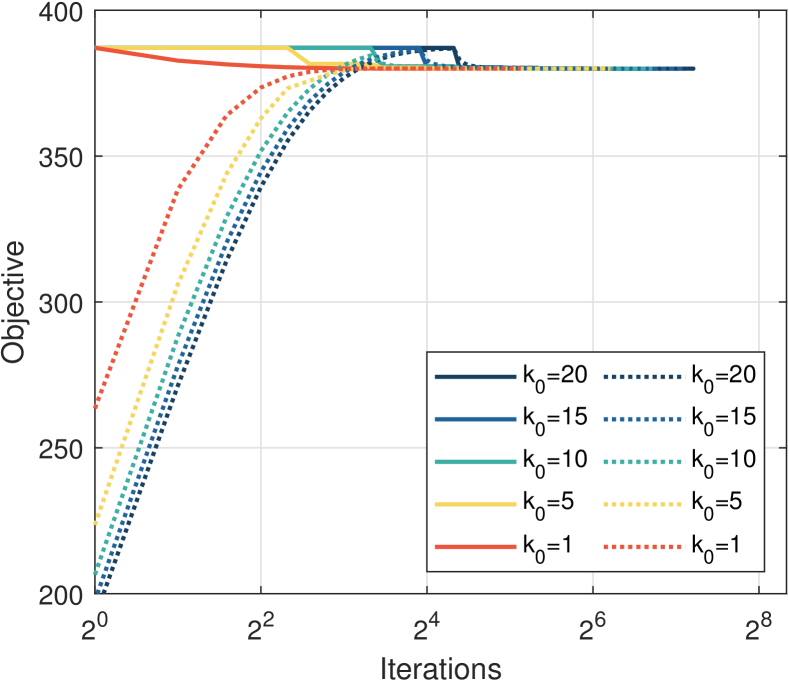
(a) CEADMM solving Ex. 5.1

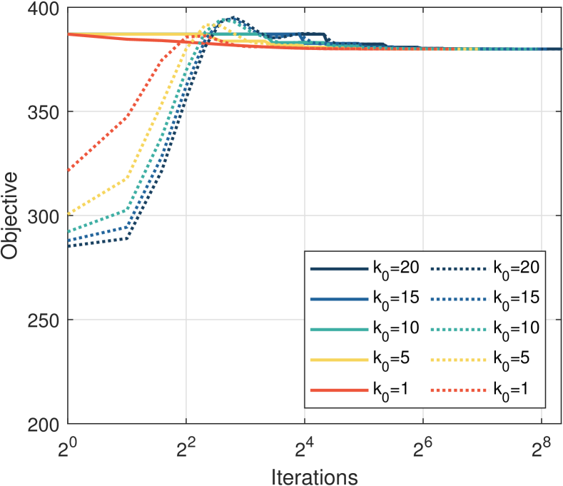
(b) ICEADMM solving Ex. 5.1

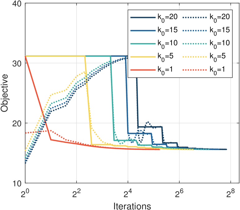
(c) ICEADMM solving Ex. 5.2

Figure 2: $f(\mathbf{y}^{k})$ (solid lines) and $F(X^{k})$ (dashed lines) v.s. iterations.

5.3.1 Global convergence

To see the global convergence proven in Theorems 3.1 and 4.2, we show how the objective function values decrease with iterations for CEADMM and ICEADMM under five choices of $k_{0}\in\{1,5,10,15,20\}$. Corresponding results are presented in Figure 2, where $m=90$ for Example 5.1 and $m=200$ for Example 5.2 with data qot. As expected, all lines eventually tend to the same objective function value, well testifying Theorem 3.1 that the whole sequence converges to the optimal function value of problem (2.7). It is clear that the bigger values of $k_{0}>1$ (i.e., the wider gap between two global aggregations) are, the more iterations are required to reach the optimal function value.

5.3.2 Convergence rate

To see the convergence speed of two algorithms, as stated in Theorems 3.3 and 4.3, we present two errors, $\|\nabla f(\mathbf{y}^{k})\|^{2}$ and $\|\nabla F(X^{k})\|^{2}$, in Figure 3 where $m=90$ for Example 5.1 and $m=200$ for Example 5.2 with data sct. The overall phenomena show that (i) both errors vanish gradually along with the iterations rising, (ii) the big values of $k_{0}$, the more iterations required by CEADMM to converge, which perfectly justifies Theorems 3.3 and 4.3 that the convergence rate $O(k_{0}/k)$ relies on $k_{0}$. What is more, it is clear that for the same $k_{0}$, ICEADMM takes more iterations than CEADMM to converge, such as, 240 v.s. 100 iterations shown in curves of $k_{0}=10$ in Figures 3(a) and 3(b).

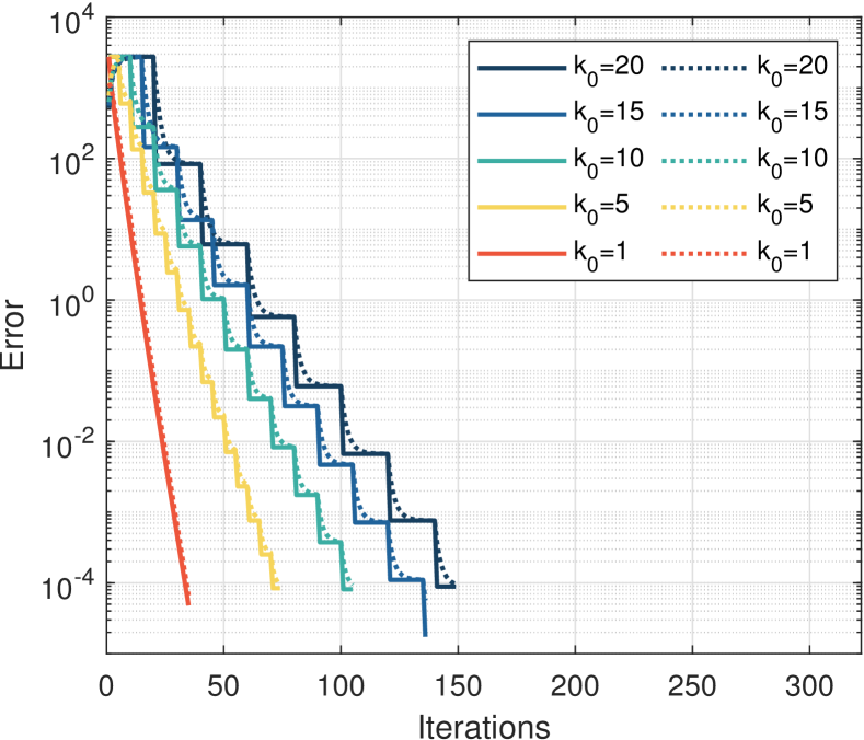
(a) CEADMM solving Ex. 5.1

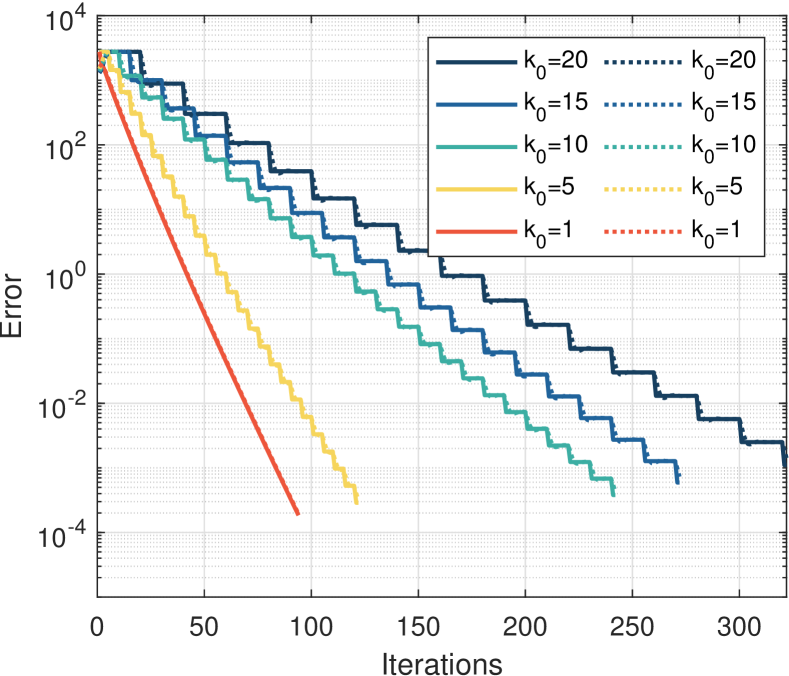
(b) ICEADMM solving Ex. 5.1

(c) ICEADMM solving Ex. 5.2

Figure 3: $\|\nabla f(\mathbf{y}^{k})\|^{2}$ (solid lines) and $\|\nabla F(X^{k})\|^{2}$ (dashed lines) v.s. iterations.

5.3.3 Effect of $k_{0}$

Next, we would like to see how the choices of $k_{0}$ impact the performance of the two algorithms. To proceed with that, for each dimension $(m,n,d_{1},\ldots,d_{m})$ of dataset A, we generate 20 instances solved by the algorithm with a fixed $k_{0}\in[20]$ and present the average results in Figure 4, where the following comments can be declared:

(a) CEADMM solving Example 5.1. From Figures 4(a) to 4(b), with increasing $k_{0}$, the total number of iterations is increasing but communication rounds are decreasing. That is, CEADMM with $k_{0}>1$ takes fewer global aggregations than the standard ADMM. For example, when $m=30$ in Figure 4(e), IADMM requires 118 rounds of communications while ICEADMM with $k_{0}=20$ only needs approximately 20 rounds. To this end, it is much more efficient than IADMM in terms of saving communication costs.

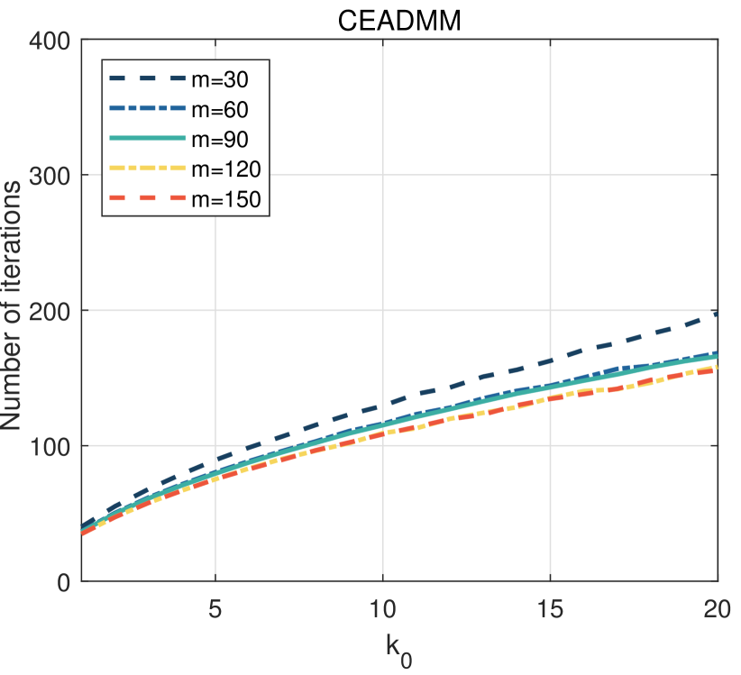
(a) Number of iterations

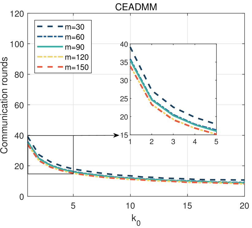
(b) Communication rounds

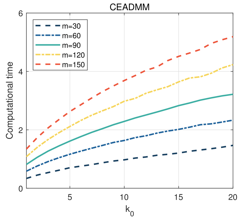
(c) Computational time

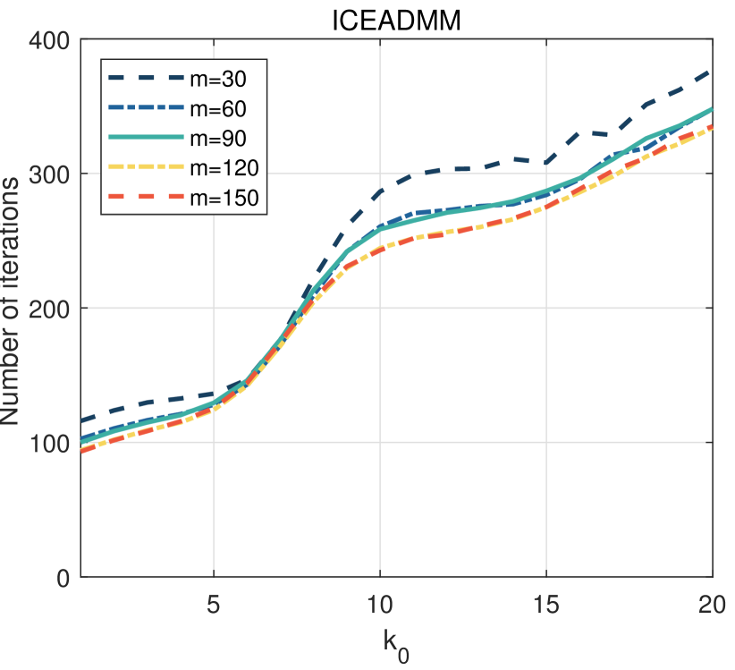
(d) Number of iterations

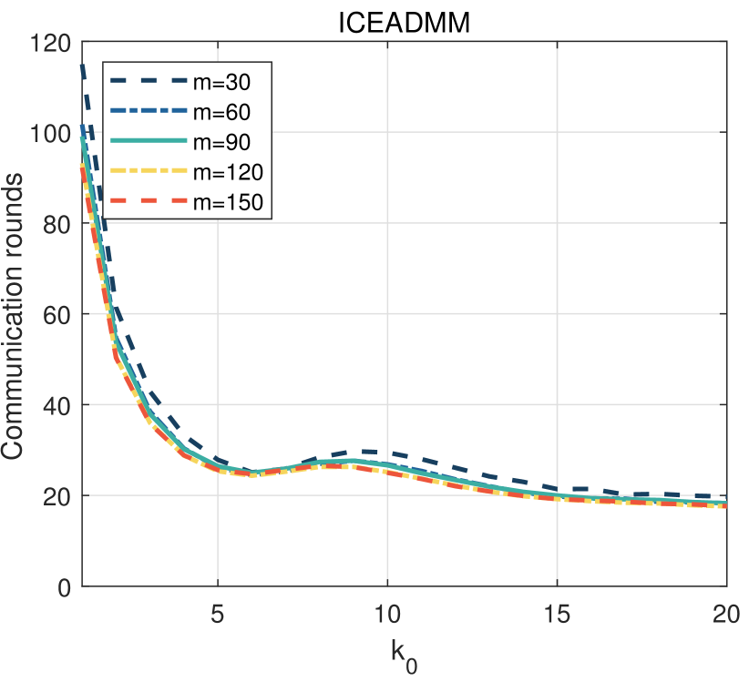
(e) Communication rounds

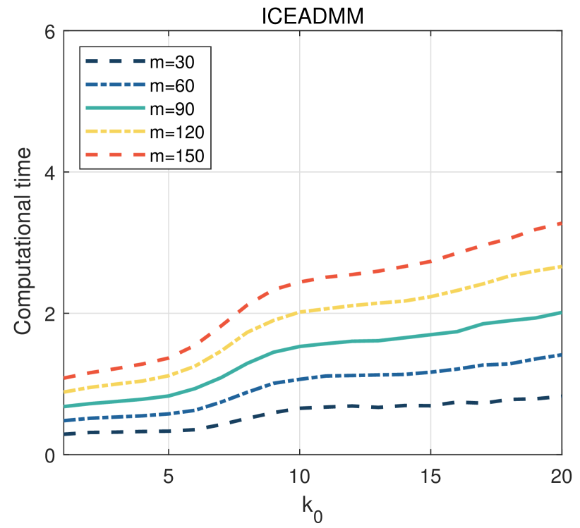
(f) Computational time

Figure 4: Effect of $k_{0}$ for Example 5.1.

Since we conducted the numerical experiments on a single laptop, the total computational time relies on the number of iterations. The curves in Figure 4(c) show that the bigger values of $k_{0}$, the longer time because bigger $k_{0}$ results in more iterations, as shown in Figure 4(a). Suppose that if the local updates (i.e., (3.4) and (3.6)) of CEADMM are implemented on different local devices, such as cellphones, laptops, or desktops, then we must take the price of communications between the local devices and the central server into consideration since more communications lead to an extremely higher price. Hence, it is necessary to reduce the number of global aggregations, that is, to set a properly bigger $k_{0}$.

(b) ICEADMM solving Example 5.1. Corresponding results presented in Figures 4(d) - 4(f) are similar to those in Figures 4(a) - 4(c). Again, the total number of iterations and computational time are rising but communication rounds are declining along with $k_{0}$ ascending. Once again, ICEADMM with $k_{0}>1$ is more communication-efficient than the standard IADMM since it executes much fewer global aggregations.

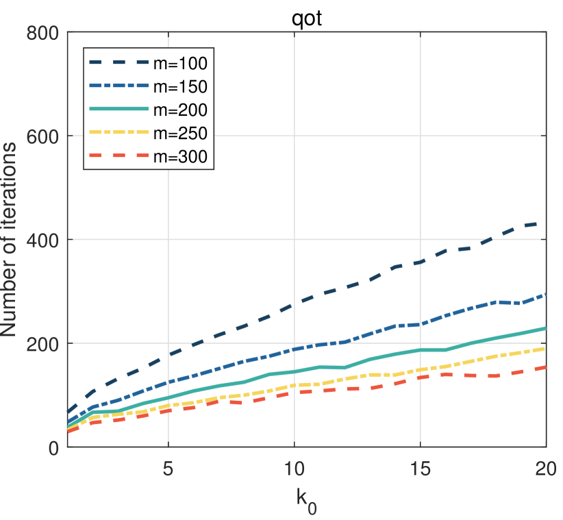
(a) Number of iterations

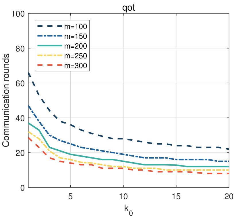
(b) Communication rounds

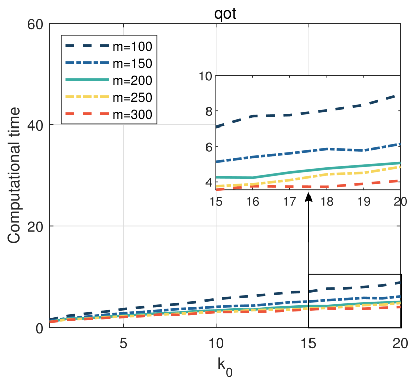
(c) Computational time

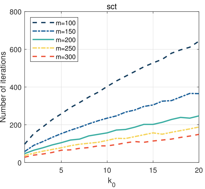
(d) Number of iterations

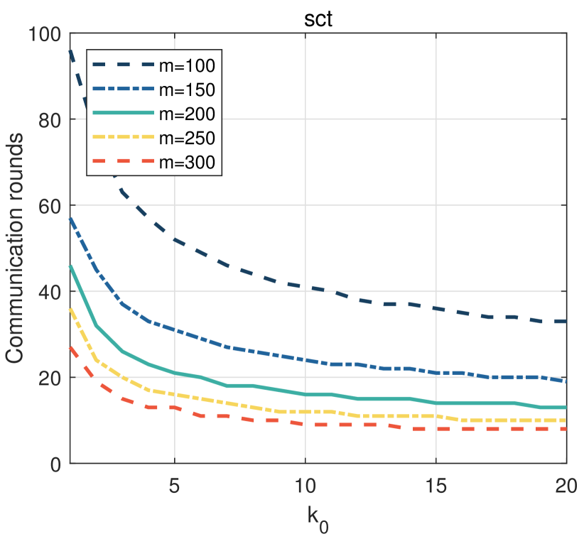
(e) Communication rounds

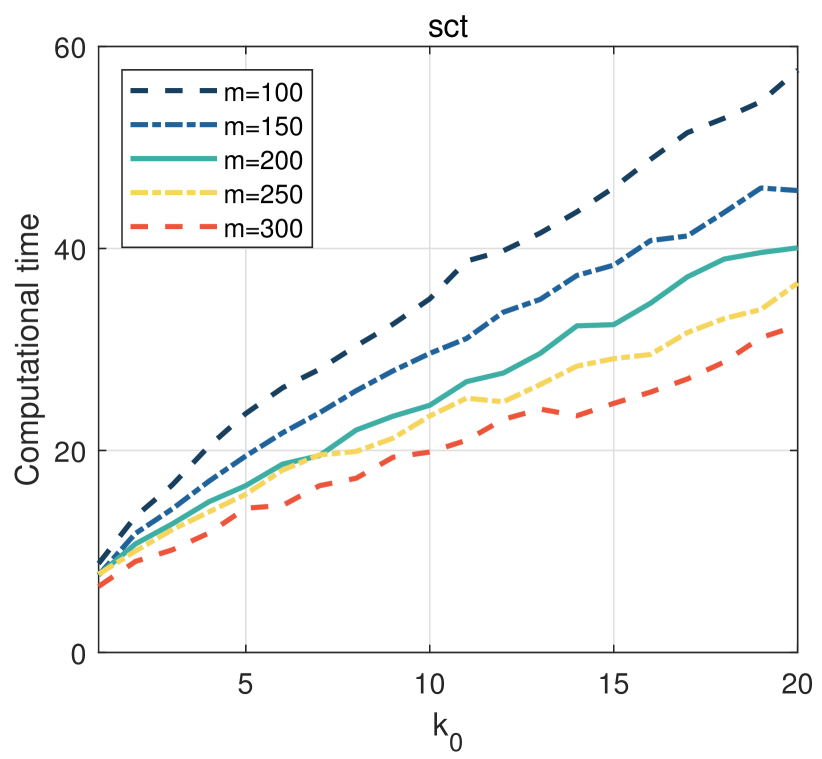
(f) Computational time

Figure 5: Effect of $k_{0}$ for Example 5.2.

(c) ICEADMM solving Example 5.2. Figure 5 demonstrates that there is no big difference with Figure 4. Moreover, the bigger $m$ (i.e., the more clients), the fewer number of iterations consumed to converge, leading to the shorter computational time. Once again, the larger $k_{0}$ results in the lower communication rounds, displaying the higher communication efficiency.

6 Conclusion

This paper developed two ADMM-based federated learning algorithms and managed to address three issues in federated learning, including saving communication resources, reducing computational complexity, and establishing convergence property under very reasonable assumptions. These advantages hint that the proposed algorithms might be practical to deal with many real applications such as mobile edge computing [35, 36], over-the-air computation [37, 38], vehicular communications [1], unmanned aerial vehicle online path control [39] and so forth. Moreover, we feel that the algorithmic schemes and techniques used to build the convergence theory could be also valid for tackling decentralized federated learning [28, 40]. We leave these as future research.

7 Appendix

For notational simplicity, hereafter, we denote

$$\qquad\begin{array}[]{llllll}\triangle\mathbf{y}^{k+1}:=\mathbf{y}^{k+1}-\mathbf{y}^{k},\qquad\triangle\mathbf{x}_{i}^{k+1}:=\mathbf{x}_{i}^{k+1}-\mathbf{x}_{i}^{k},\qquad\triangle{\boldsymbol{\pi}}_{i}^{k+1}:={\boldsymbol{\pi}}_{i}^{k+1}-\mathbf{x}_{i}^{k},\end{array}$$

and let $\mathbf{a}^{k}\rightarrow\mathbf{a}$ stand for $\lim_{k\rightarrow\infty}\mathbf{a}^{k}=\mathbf{a}$. For any vectors $\mathbf{a},\mathbf{b}$, and $\mathbf{a}_{i}$, we have

$$\begin{array}[]{rcl}-\|\mathbf{b}\|^{2}&=&2\langle\mathbf{a},\mathbf{b}\rangle+\|\mathbf{a}\|^{2}-\|\mathbf{a}+\mathbf{b}\|^{2},\\ \|\mathbf{a}+\mathbf{b}\|^{2}&\leq&(1+t)\|\mathbf{a}\|^{2}+(1+\frac{1}{t})\|\mathbf{b}\|^{2},~{}\forall~{}t>0,\\ \|\sum_{i=1}^{m}\mathbf{a}_{i}\|^{2}&\leq&m\sum_{i=1}^{m}\|\mathbf{a}_{i}\|^{2}.\end{array}$$ (7.5)

The gradient Lipschitz continuity in (1.1) with a Lipschitz constant $r>0$ indicates that

$$\begin{array}[]{l}f(\mathbf{x})\leq f(\mathbf{z})+\langle\nabla f(\mathbf{z}),\mathbf{x}-\mathbf{z}\rangle+\frac{r}{2}\|\mathbf{x}-\mathbf{z}\|^{2},\end{array}$$ (7.7)

for any $\mathbf{x},\mathbf{z}\in\mathbb{R}^{n}$. Hence, there exists $H$ such that $rI\succeq H\succeq 0$ and

$$\begin{array}[]{l}f(\mathbf{x})\leq f(\mathbf{z})+\langle\nabla f(\mathbf{z}),\mathbf{x}-\mathbf{z}\rangle+\frac{1}{2}\|\mathbf{x}-\mathbf{z}\|^{2}_{H}.\end{array}$$ (7.9)

The above condition immediately implies

$$\qquad\begin{array}[]{llll}\langle\nabla f(\mathbf{x})-\nabla f(\mathbf{z}),\mathbf{x}-\mathbf{z}\rangle&\leq&\|\mathbf{x}-\mathbf{z}\|^{2}_{H}.\end{array}$$ (7.11)

A special case of $f$ is a quadratic function and $H=\nabla^{2}f$, the Hessian matrix of $f$. It follows from the Mean Value Theorem that, for any $\mathbf{x}$ and $\mathbf{z}$,

$$\begin{array}[]{llll}f(\mathbf{x})-f(\mathbf{z})-\langle\nabla f(\mathbf{x}),\mathbf{x}-\mathbf{z}\rangle&=&\int_{0}^{1}df(\mathbf{z}+t(\mathbf{x}-\mathbf{z}))-\langle\nabla f(\mathbf{x}),\mathbf{x}-\mathbf{z}\rangle\\ &=&\int_{0}^{1}\langle\nabla f(\mathbf{z}+t(\mathbf{x}-\mathbf{z}))-\nabla f(\mathbf{x}),\mathbf{x}-\mathbf{z}\rangle dt\\ &\leq&\int_{0}^{1}r\|\mathbf{z}+t(\mathbf{x}-\mathbf{z}))-\mathbf{x}\|\|\mathbf{x}-\mathbf{z}\|dt\\ &=&r\|\mathbf{x}-\mathbf{z}\|^{2}\int_{0}^{1}(1-t)dt\\ &=&\frac{r}{2}\|\mathbf{x}-\mathbf{z}\|^{2}.\end{array}$$ (7.17)

7.1 Proofs of all theorems in Section 3

Lemma 7.1.

Let $\{(\mathbf{y}^{k},X^{k},\Pi^{k})\}$ be the sequence generated by Algorithm 3. If Assumption 3.1 holds, then for any $k\geq 0$,

$$\begin{array}[]{lll}\mathcal{L}^{k+1}-\mathcal{L}^{k}\leq-\frac{\sigma}{2}\|\triangle\mathbf{y}^{k+1}\|^{2}-\sum_{i=1}^{m}\frac{\theta_{i}}{2}\|\triangle\mathbf{x}_{i}^{k+1}\|^{2},\end{array}$$ (7.19)

where $\theta_{i}$ is given by

$$\begin{array}[]{lll}\theta_{i}:=\sigma_{i}-w_{i}r_{i}-{2w_{i}^{2}r_{i}^{2}}/{\sigma_{i}},\qquad i\in[m].\end{array}$$ (7.21)

Proof.

The optimality condition for (3.2) is

$$\begin{array}[]{lcl}\forall~{}k\in\mathcal{K}:~{}~{}0&=&\sum_{i=1}^{m}[-{\boldsymbol{\pi}}_{i}^{k}+\sigma_{i}(\mathbf{x}^{k+1}-\mathbf{x}_{i}^{k})]\\ &\overset{\eqref{ceadmm-sub3}}{=}&\sum_{i=1}^{m}[-{\boldsymbol{\pi}}_{i}^{k+1}+\sigma_{i}(\mathbf{x}_{i}^{k+1}-\mathbf{y}^{k+1})]+\sum_{i=1}^{m}[\sigma_{i}(\mathbf{x}^{k+1}-\mathbf{x}_{i}^{k})]\\ &=&\sum_{i=1}^{m}[-{\boldsymbol{\pi}}_{i}^{k+1}+\sigma_{i}(\mathbf{x}_{i}^{k+1}-\mathbf{x}_{i}^{k})],\end{array}$$ (7.25)

where the last equation holds from $\mathbf{y}^{k+1}=\mathbf{x}^{k+1},k\in\mathcal{K}$. The optimality condition for (3.4) is

$$\begin{array}[]{lcl}\forall~{}k\geq 0:~{}~{}0={\boldsymbol{g}}_{i}^{k+1}+{\boldsymbol{\pi}}_{i}^{k}+\sigma_{i}(\mathbf{x}_{i}^{k+1}-\mathbf{y}^{k+1})\overset{\eqref{ceadmm-sub3}}{=}{\boldsymbol{g}}_{i}^{k+1}+{\boldsymbol{\pi}}_{i}^{k+1},\qquad\forall~{}i\in[m].\end{array}$$ (7.27)

The gap of the left-hand side of (7.19) can be decomposed as

$$\qquad\begin{array}[]{llllll}\mathcal{L}^{k+1}-\mathcal{L}^{k}=:e_{1}^{k}+e_{2}^{k}+e_{3}^{k},\end{array}$$ (7.29)

with

$$\begin{array}[]{llllll}e_{1}^{k}&:=&\mathcal{L}(\mathbf{y}^{k+1},X^{k},\Pi^{k})-\mathcal{L}^{k},\\ e_{2}^{k}&:=&\mathcal{L}(\mathbf{y}^{k+1},X^{k+1},\Pi^{k})-\mathcal{L}(\mathbf{y}^{k+1},X^{k},\Pi^{k}),\\ e_{3}^{k}&:=&\mathcal{L}^{k+1}-\mathcal{L}(\mathbf{y}^{k+1},X^{k+1},\Pi^{k}).\end{array}$$ (7.33)

To estimate $e_{1}^{k}$, if $k\notin\mathcal{K}$, then from (3.9), we have $\mathbf{y}^{k+1}=\mathbf{x}^{\tau_{k}+1}=\mathbf{y}^{k}$, thereby leading to

$$\begin{array}[]{lll}e_{1}^{k}=\mathcal{L}(\mathbf{y}^{k+1},X^{k},\Pi^{k})-\mathcal{L}^{k}=0=-\frac{\sigma}{2}\|\triangle\mathbf{y}^{k+1}\|^{2}.\end{array}$$ (7.35)

If $k\in\mathcal{K}$, then (3.9) indicates $\mathbf{y}^{k+1}=\mathbf{x}^{k+1}$. Moreover, multiplying both sides of the first equation in (7.25) by $\triangle\mathbf{y}^{k+1}$ gives rise to

$$\begin{array}[]{lll}\sum_{i=1}^{m}\langle\triangle\mathbf{y}^{k+1},{\boldsymbol{\pi}}_{i}^{k}\rangle=\sum_{i=1}^{m}\langle\triangle\mathbf{y}^{k+1},\sigma_{i}(\mathbf{y}^{k+1}-\mathbf{x}_{i}^{k})\rangle.\end{array}$$ (7.37)

These facts also allow us to derive that

$$\begin{array}[]{lcl}e_{1}^{k}&\overset{\eqref{FL-opt-ver11}}{=}&\sum_{i=1}^{m}(L(\mathbf{y}^{k+1},\mathbf{x}_{i}^{k},{\boldsymbol{\pi}}_{i}^{k})-L(\mathbf{y}^{k},\mathbf{x}_{i}^{k},{\boldsymbol{\pi}}_{i}^{k}))\\ &\overset{\eqref{Def-L}}{=}&\sum_{i=1}^{m}(\langle\triangle\mathbf{y}^{k+1},-{\boldsymbol{\pi}}_{i}^{k}\rangle+\frac{\sigma_{i}}{2}\|\mathbf{x}_{i}^{k}-\mathbf{y}^{k+1}\|^{2}-\frac{\sigma_{i}}{2}\|\mathbf{x}_{i}^{k}-\mathbf{y}^{k}\|^{2})\\ &\overset{\eqref{opt-con-xk2}}{=}&\sum_{i=1}^{m}(\langle\triangle\mathbf{y}^{k+1},\sigma_{i}(\mathbf{x}_{i}^{k}-\mathbf{y}^{k+1})\rangle+\frac{\sigma_{i}}{2}\|\mathbf{x}_{i}^{k}-\mathbf{y}^{k+1}\|^{2}-\frac{\sigma_{i}}{2}\|\mathbf{x}_{i}^{k}-\mathbf{y}^{k}\|^{2})\\ &\overset{\eqref{two-vecs}}{=}&\sum_{i=1}^{m}(-\frac{\sigma_{i}}{2}\|\triangle\mathbf{y}^{k+1}\|^{2})\\ &\overset{\eqref{sum-sigma-i}}{=}&-\frac{\sigma}{2}\|\triangle\mathbf{y}^{k+1}\|^{2}.\end{array}$$ (7.43)

To estimate $e_{2}^{k}$, we have the following chain of inequalities,

$$\begin{array}[]{lcl}&&L(\mathbf{y}^{k+1},\mathbf{x}_{i}^{k+1},{\boldsymbol{\pi}}_{i}^{k})-L(\mathbf{y}^{k+1},\mathbf{x}_{i}^{k},{\boldsymbol{\pi}}_{i}^{k})\\ &\overset{\eqref{Def-L}}{=}&w_{i}f_{i}(\mathbf{x}_{i}^{k+1})-w_{i}f_{i}(\mathbf{x}_{i}^{k})+\langle\triangle\mathbf{x}_{i}^{k+1},{\boldsymbol{\pi}}_{i}^{k}\rangle+\frac{\sigma_{i}}{2}\|\mathbf{x}_{i}^{k+1}-\mathbf{y}^{k+1}\|^{2}-\frac{\sigma_{i}}{2}\|\mathbf{x}_{i}^{k}-\mathbf{y}^{k+1}\|^{2}\\ &\overset{\eqref{H-Lip-continuity-fxy}}{\leq}&\langle\triangle\mathbf{x}_{i}^{k+1},{\boldsymbol{g}}_{i}^{k+1}+{\boldsymbol{\pi}}_{i}^{k}\rangle+\frac{w_{i}r_{i}}{2}\|\triangle\mathbf{x}_{i}^{k+1}\|^{2}+\frac{\sigma_{i}}{2}\|\mathbf{x}_{i}^{k+1}-\mathbf{y}^{k+1}\|^{2}-\frac{\sigma_{i}}{2}\|\mathbf{x}_{i}^{k}-\mathbf{y}^{k+1}\|^{2}\\ &\overset{\eqref{opt-con-xik1}}{=}&\langle\triangle\mathbf{x}_{i}^{k+1},\sigma_{i}(\mathbf{y}^{k+1}-\mathbf{x}_{i}^{k+1})\rangle+\frac{w_{i}r_{i}}{2}\|\triangle\mathbf{x}_{i}^{k+1}\|^{2}+\frac{\sigma_{i}}{2}\|\mathbf{x}_{i}^{k+1}-\mathbf{y}^{k+1}\|^{2}-\frac{\sigma_{i}}{2}\|\mathbf{x}_{i}^{k}-\mathbf{y}^{k+1}\|^{2}\\ &\overset{\eqref{two-vecs}}{=}&-\frac{\sigma_{i}-w_{i}r_{i}}{2}\|\triangle\mathbf{x}_{i}^{k+1}\|^{2},\end{array}$$

which leads to

$$\begin{array}[]{lllll}e_{2}^{k}&=&\sum_{i=1}^{m}(L(\mathbf{y}^{k+1},\mathbf{x}_{i}^{k+1},{\boldsymbol{\pi}}_{i}^{k})-L(\mathbf{y}^{k+1},\mathbf{x}_{i}^{k},{\boldsymbol{\pi}}_{i}^{k}))\leq\sum_{i=1}^{m}-\frac{\sigma_{i}-w_{i}r_{i}}{2}\|\triangle\mathbf{x}_{i}^{k+1}\|^{2}.\end{array}$$ (7.46)

To estimate $e_{3}^{k}$, the gradient Lipschitz continuity delivers that, for any $i\in[m]$,

$$\begin{array}[]{lll}\|\triangle{\boldsymbol{\pi}}_{i}^{k+1}\|\overset{\eqref{opt-con-xik1}}{=}\|-{\boldsymbol{g}}_{i}^{k+1}+{\boldsymbol{g}}_{i}^{k}\|\overset{\eqref{Lip-r}}{\leq}w_{i}r_{i}\|\triangle\mathbf{x}_{i}^{k+1}\|.\end{array}$$ (7.48)

This condition suffices to the following chain of inequalities,

$$\begin{array}[]{lcl}e_{3}^{k}&=&\mathcal{L}^{k+1}-\sum_{i=1}^{m}L(\mathbf{y}^{k+1},\mathbf{x}_{i}^{k+1},{\boldsymbol{\pi}}_{i}^{k})\\ &\overset{\eqref{Def-L}}{=}&\sum_{i=1}^{m}\langle\mathbf{x}_{i}^{k+1}-\mathbf{y}^{k+1},\triangle{\boldsymbol{\pi}}_{i}^{k+1}\rangle\\ &\overset{\eqref{ceadmm-sub3}}{=}&\sum_{i=1}^{m}\frac{1}{\sigma_{i}}\|\triangle{\boldsymbol{\pi}}_{i}^{k+1}\|^{2}\\ &\overset{\eqref{Lip-fi}}{\leq}&\sum_{i=1}^{m}\frac{w_{i}^{2}r_{i}^{2}}{\sigma_{i}}\|\triangle\mathbf{x}_{i}^{k+1}\|^{2},\end{array}$$ (7.53)

Overall, combining (7.29), (7.35), (7.43), (7.46) and (7.53), we conclude (7.19) immediately. ∎

Lemma 7.2.

Let $\{(\mathbf{y}^{k},X^{k},\Pi^{k})\}$ be the sequence generated by Algorithm 3 with $\sigma_{i}>2w_{i}r_{i}$ for every $i\in[m]$. The following results hold under Assumption 3.1.

• $\{\mathcal{L}^{k}\}$ is non-increasing.

• $\mathcal{L}^{k}\geq f(\mathbf{y}^{k})\geq f^{*}>-\infty$ for any integer $k\geq 0$.

• The limits of all the following terms are zero, namely,

  $$\begin{array}[]{lll}\underset{k\rightarrow\infty}{\lim}\triangle\mathbf{y}^{k+1}&=&\underset{k\rightarrow\infty}{\lim}\triangle\mathbf{x}^{k+1}_{i}=\underset{k\rightarrow\infty}{\lim}\triangle{\boldsymbol{\pi}}_{i}^{k+1}\\ &=&\underset{k\rightarrow\infty}{\lim}(\mathbf{x}_{i}^{k+1}-\mathbf{y}^{k+1})=\underset{k\rightarrow\infty}{\lim}(\mathbf{x}_{i}^{k+1}-\mathbf{x}_{i}^{\tau_{k}+1})=0.\end{array}$$ (7.56)

Proof.

i) The conclusion follows from (7.19) and $\theta_{i}>0$ (due to $\sigma_{i}>2w_{i}r_{i}$) immediately.

ii) The gradient Lipschitz continuity of $f_{i}$ implies

$$\begin{array}[]{lllll}w_{i}f_{i}(\mathbf{y}^{k+1})-w_{i}f_{i}(\mathbf{x}_{i}^{k+1})&\overset{\eqref{Lip-r/2}}{\leq}&\langle\mathbf{y}^{k+1}-\mathbf{x}_{i}^{k+1},{\boldsymbol{g}}_{i}^{k+1}\rangle+\frac{r_{i}w_{i}}{2}\|\mathbf{x}_{i}^{k+1}-\mathbf{y}^{k+1}\|^{2}\\ &\overset{\eqref{opt-con-xik1}}{=}&\langle\mathbf{y}^{k+1}-\mathbf{x}_{i}^{k+1},-{\boldsymbol{\pi}}_{i}^{k+1}\rangle+\frac{r_{i}w_{i}}{2}\|\mathbf{x}_{i}^{k+1}-\mathbf{y}^{k+1}\|^{2},\end{array}$$

which by $\sigma_{i}>2w_{i}r_{i}$ allows us to obtain

$$\begin{array}[]{lll}\mathcal{L}^{k+1}&=&\sum_{i=1}^{m}L(\mathbf{y}^{k+1},\mathbf{x}_{i}^{k+1},{\boldsymbol{\pi}}_{i}^{k+1})\\ &=&\sum_{i=1}^{m}(w_{i}f_{i}(\mathbf{x}_{i}^{k+1})+\langle\mathbf{x}_{i}^{k+1}-\mathbf{y}^{k+1},{\boldsymbol{\pi}}_{i}^{k+1}\rangle)+\sum_{i=1}^{m}\frac{\sigma_{i}}{2}\|\mathbf{x}_{i}^{k+1}-\mathbf{y}^{k+1}\|^{2}\\ &\geq&\sum_{i=1}^{m}(w_{i}f_{i}(\mathbf{y}^{k+1})+\frac{\sigma_{i}-w_{i}r_{i}}{2}\|\mathbf{x}_{i}^{k+1}-\mathbf{y}^{k+1}\|^{2})\\ &\geq&\sum_{i=1}^{m}w_{i}f_{i}(\mathbf{y}^{k+1})=f(\mathbf{y}^{k+1})\\ &\geq&f^{*}\overset{\eqref{FL-opt-lower-bound}}{>}-\infty.\end{array}$$ (7.63)

iii) It follows from (7.19) that

$$\begin{array}[]{lcl}{\sum}_{k\geq 0}\Big{[}\frac{\sigma}{2}\|\vartriangle\mathbf{y}^{k+1}\|^{2}+~{}\sum_{i=1}^{m}\frac{\theta_{i}}{2}\|\triangle\mathbf{x}^{k+1}_{i}\|^{2}\Big{]}&\leq&{\sum}_{k\geq 0}(\mathcal{L}^{k}-\mathcal{L}^{k+1})\\ &=&\mathcal{L}^{0}-{\lim}_{k\rightarrow\infty}\mathcal{L}^{k+1}\overset{\eqref{lower-bound-L}}{<}+\infty.\end{array}$$

The above condition means $\|\triangle\mathbf{y}^{k+1}\|\rightarrow 0$ and $\|\triangle\mathbf{x}^{k+1}_{i}\|\rightarrow 0,$ yielding $\|\triangle{\boldsymbol{\pi}}_{i}^{k+1}\|\rightarrow 0$ by (7.48). This contributes to

$$\begin{array}[]{llll}~{}~{}{\lim}_{k\rightarrow\infty}\|\sigma_{i}(\mathbf{x}_{i}^{k+1}-\mathbf{y}^{k+1})\|\overset{\eqref{ceadmm-sub3}}{=}{\lim}_{k\rightarrow\infty}\|\triangle{\boldsymbol{\pi}}_{i}^{k+1}\|=0.\end{array}$$

Since $\tau_{k}\leq k<\tau_{k}+k_{0}$, we have $\mathbf{y}^{k+1}=\mathbf{x}^{\tau_{k}+1}=\mathbf{y}^{\tau_{k}+1}$ from (3.9). As a result,

$$\begin{array}[]{lcl}\|\sigma_{i}(\mathbf{x}^{k+1}_{i}-\mathbf{x}^{\tau_{k}+1}_{i})\|^{2}&=&\|\sigma_{i}(\mathbf{x}^{k+1}_{i}-\mathbf{y}^{k+1}+\mathbf{y}^{\tau_{k}+1}-\mathbf{x}^{\tau_{k}+1}_{i})\|^{2}\\ &\overset{\eqref{two-vecs}}{\leq}&2\|\sigma_{i}(\mathbf{x}^{k+1}_{i}-\mathbf{y}^{k+1})\|^{2}+2\|\sigma_{i}(\mathbf{y}^{\tau_{k}+1}-\mathbf{x}^{\tau_{k}+1}_{i})\|^{2}\\ &\overset{\eqref{ceadmm-sub3}}{=}&2\|\triangle{\boldsymbol{\pi}}^{k+1}_{i}\|^{2}+2\|\triangle{\boldsymbol{\pi}}^{\tau_{k}+1}_{i}\|^{2},\end{array}$$ (7.69)

which together with $\triangle{\boldsymbol{\pi}}^{k+1}_{i}\rightarrow 0$ yields $(\mathbf{x}^{k+1}_{i}-\mathbf{x}^{\tau_{k}+1}_{i})\rightarrow 0$. Hence, the whole proof is finished. ∎

7.1.1 Proof of Theorem 3.1

Proof.

i) It follows from Lemma 7.2 that $\{\mathcal{L}^{k}\}$ is non-increasing and bounded from below. Therefore, the whole sequence $\{\mathcal{L}^{k}\}$ converges. Since

$$\begin{array}[]{lcl}\mathcal{L}^{k}-F(X^{k})&\overset{\eqref{FL-opt-ver11}}{=}&\sum_{i=1}^{m}(\langle\mathbf{x}_{i}^{k}-\mathbf{y}^{k},{\boldsymbol{\pi}}_{i}^{k}\rangle+\frac{\sigma_{i}}{2}\|\mathbf{x}_{i}^{k}-\mathbf{y}^{k}\|^{2})\\ &\overset{\eqref{ceadmm-sub3}}{=}&\sum_{i=1}^{m}(\frac{1}{\sigma_{i}}\langle\triangle{\boldsymbol{\pi}}_{i}^{k},{\boldsymbol{\pi}}_{i}^{k}\rangle+\frac{1}{2\sigma_{i}}\|\triangle{\boldsymbol{\pi}}_{i}^{k}\|^{2})\\ &{=}&\sum_{i=1}^{m}(\frac{1}{2\sigma_{i}}\|{\boldsymbol{\pi}}_{i}^{k}\|^{2}-\frac{1}{2\sigma_{i}}\|{\boldsymbol{\pi}}_{i}^{k-1}\|^{2}+\frac{1}{\sigma_{i}}\|\triangle{\boldsymbol{\pi}}_{i}^{k}\|^{2}),\end{array}$$ (7.73)

and $\triangle{\boldsymbol{\pi}}_{i}^{k}\rightarrow 0$ in (7.56), we obtain

$$\qquad\begin{array}[]{lll}{\lim}_{k\rightarrow\infty}F(X^{k})={\lim}_{k\rightarrow\infty}\mathcal{L}^{k}.\end{array}$$

It follows from Mean Value Theory that

$$f_{i}(\mathbf{y}^{k})=f_{i}(\mathbf{x}_{i}^{k})+\langle\mathbf{y}^{k}-\mathbf{x}_{i}^{k},\nabla f_{i}(\mathbf{x}_{i}^{k}(\alpha))\rangle,$$

where $\mathbf{x}_{i}^{k}(\alpha):=(1-\alpha)\mathbf{y}^{k}+\alpha\mathbf{x}_{i}^{k}$ for some $\alpha\in(0,1)$. The above relation results in

$$\begin{array}[]{lll}w_{i}f_{i}(\mathbf{x}_{i}^{k})+\langle\mathbf{x}_{i}^{k}-\mathbf{y}^{k},{\boldsymbol{\pi}}_{i}^{k}\rangle&\overset{\eqref{opt-con-xik1}}{=}&w_{i}f_{i}(\mathbf{x}_{i}^{k})+\langle\mathbf{x}_{i}^{k}-\mathbf{y}^{k},-{\boldsymbol{g}}_{i}^{k}\rangle\\ &=&w_{i}f_{i}(\mathbf{y}^{k})+\langle\mathbf{x}_{i}^{k}-\mathbf{y}^{k},w_{i}\nabla f_{i}(\mathbf{x}_{i}^{k}(\alpha))-{\boldsymbol{g}}_{i}^{k}\rangle.\end{array}$$ (7.77)

The gradient Lipschitz continuity of $f_{i}$ yields that

$$\begin{array}[]{lll}\|w_{i}\nabla f_{i}(\mathbf{x}_{i}^{k}(\alpha))-{\boldsymbol{g}}_{i}^{k}\|&\leq&w_{i}r_{i}\|\mathbf{x}_{i}^{k}(\alpha)-\mathbf{x}_{i}^{k}\|=w_{i}r_{i}(1-\alpha)\|\mathbf{y}^{k}-\mathbf{x}_{i}^{k}\|,\end{array}$$

which by $(\mathbf{y}^{k}-\mathbf{x}_{i}^{k})\rightarrow 0$ in (7.56) leads to

$$\begin{array}[]{lll}&&\lim_{k\rightarrow\infty}(w_{i}\nabla f_{i}(\mathbf{x}_{i}^{k}(\alpha))-{\boldsymbol{g}}_{i}^{k})=0.\end{array}$$

This, (7.77) and $(\mathbf{y}^{k}-\mathbf{x}_{i}^{k})\rightarrow 0$ bring out

$$\begin{array}[]{lll}\lim_{k\rightarrow\infty}(w_{i}f_{i}(\mathbf{x}_{i}^{k})+\langle\mathbf{x}_{i}^{k}-\mathbf{y}^{k},{\boldsymbol{\pi}}_{i}^{k}\rangle)=\lim_{k\rightarrow\infty}w_{i}f_{i}(\mathbf{y}^{k}).\end{array}$$

The above fact and (7.56) enable us to obtain

$$\begin{array}[]{lll}{\lim}_{k\rightarrow\infty}\mathcal{L}^{k}&=&{\lim}_{k\rightarrow\infty}\sum_{i=1}^{m}(w_{i}f_{i}(\mathbf{x}_{i}^{k})+\langle\mathbf{x}_{i}^{k}-\mathbf{y}^{k},{\boldsymbol{\pi}}_{i}^{k}\rangle+\frac{\sigma_{i}}{2}\|\mathbf{x}_{i}^{k}-\mathbf{y}^{k}\|^{2})\\ &=&{\lim}_{k\rightarrow\infty}\sum_{i=1}^{m}w_{i}f_{i}(\mathbf{y}^{k})={\lim}_{k\rightarrow\infty}f(\mathbf{y}^{k}).\end{array}$$

ii) Direct verifications render that

$$\begin{array}[]{lcl}{\lim}_{k\rightarrow\infty}\|{\boldsymbol{\pi}}_{i}^{k+1}-{\boldsymbol{\pi}}_{i}^{\tau_{k}+1}\|&\overset{\eqref{opt-con-xik1}}{=}&{\lim}_{k\rightarrow\infty}\|-{\boldsymbol{g}}_{i}^{k+1}+{\boldsymbol{g}}_{i}^{\tau_{k}+1}\|\\ &\overset{\eqref{Lip-r}}{\leq}&{\lim}_{k\rightarrow\infty}w_{i}r_{i}\|\mathbf{x}^{k+1}_{i}-\mathbf{x}^{\tau_{k}+1}_{i}\|\\ &\overset{\eqref{limit-5-term-0}}{=}&0.\end{array}$$

Using this condition and the following one

$$\begin{array}[]{lcl}0&\overset{\eqref{opt-con-xk1}}{=}&{\lim}_{\tau_{k}\rightarrow\infty}\sum_{i=1}^{m}(-{\boldsymbol{\pi}}_{i}^{\tau_{k}+1}+\sigma_{i}\triangle\mathbf{x}_{i}^{\tau_{k}+1})\overset{\eqref{limit-5-term-0}}{=}{\lim}_{\tau_{k}\rightarrow\infty}\sum_{i=1}^{m}-{\boldsymbol{\pi}}_{i}^{\tau_{k}+1}\end{array}$$

can claim that

$$\begin{array}[]{llllllll}{\lim}_{k\rightarrow\infty}\sum_{i=1}^{m}{\boldsymbol{\pi}}_{i}^{k+1}=0.\end{array}$$ (7.85)

Taking the limit on both sides of (7.27) gives us

$$\begin{array}[]{lcl}0&=&{\lim}_{k\rightarrow\infty}\sum_{i=1}^{m}~{}({\boldsymbol{g}}_{i}^{k+1}+{\boldsymbol{\pi}}_{i}^{k+1})\\ &\overset{\eqref{limit-K-grad-pi-exact}}{=}&{\lim}_{k\rightarrow\infty}\sum_{i=1}^{m}{\boldsymbol{g}}_{i}^{k+1}={\lim}_{k\rightarrow\infty}\nabla F(X^{k+1}),\end{array}$$ (7.88)

which together with $(\mathbf{x}_{i}^{k+1}-\mathbf{y}^{k+1})\rightarrow 0$ and the gradient Lipschitz continuity yields that

$$\begin{array}[]{llllllll}0={\lim}_{k\rightarrow\infty}\sum_{i=1}^{m}w_{i}\nabla f_{i}(\mathbf{y}^{k+1})={\lim}_{k\rightarrow\infty}\nabla f(\mathbf{y}^{k+1}),\end{array}$$

completing the whole proof. ∎

7.1.2 Proof of Theorem 3.2

Proof.

i) It follows from Lemma 7.2 i) and (7.63) that

$$\begin{array}[]{lll}\mathcal{L}^{0}\geq\mathcal{L}^{k+1}\geq\sum_{i=1}^{m}w_{i}f_{i}(\mathbf{y}^{k+1})=f(\mathbf{y}^{k+1}),\end{array}$$ (7.91)

which implies $\mathbf{y}^{k+1}\in\mathcal{S}(\mathcal{L}^{0})$ and hence $\{\mathbf{y}^{k+1}\}$ is bounded due to the boundedness of $\mathcal{S}(\mathcal{L}^{0})$. This calls forth the boundedness of $\{\mathbf{x}_{i}^{k+1}\}$ as $(\mathbf{x}_{i}^{k+1}-\mathbf{y}^{k+1})\rightarrow 0$ from (7.56). The boundedness of $\{{\boldsymbol{\pi}}_{i}^{k+1}\}$ can be ensured because of

$$\begin{array}[]{lcl}\|{\boldsymbol{\pi}}_{i}^{k+1}\|\overset{\eqref{opt-con-xik1}}{=}\|{\boldsymbol{g}}_{i}^{k+1}\|\leq\|{\boldsymbol{g}}_{i}^{k+1}-{\boldsymbol{g}}_{i}^{0}\|+\|{\boldsymbol{g}}_{i}^{0}\|\overset{\eqref{Lip-r}}{\leq}w_{i}r_{i}\|\mathbf{x}^{k+1}_{i}-\mathbf{x}^{0}_{i}\|+\|{\boldsymbol{g}}_{i}^{0}\|<+\infty,\end{array}$$

where ‘$<$’ is from the boundedness of $\{\mathbf{x}_{i}^{k+1}\}$. Overall, sequence $\{(\mathbf{y}^{k+1},X^{k+1},\Pi^{k+1})\}$ is bounded. Let $(\mathbf{y}^{\infty},X^{\infty},\Pi^{\infty})$ be any accumulating point of the sequence, it follows from (7.88), (7.85), and $(\mathbf{x}_{i}^{k+1}-\mathbf{y}^{k+1})\rightarrow 0$ that

$$\begin{array}[]{l}0=w_{i}\nabla f_{i}(\mathbf{x}^{\infty}_{i})+{\boldsymbol{\pi}}_{i}^{\infty}=\sum_{i=1}^{m}{\boldsymbol{\pi}}_{i}^{\infty}=\mathbf{x}^{\infty}_{i}-\mathbf{y}^{\infty}.\end{array}$$

Therefore, recalling (2.49), $(\mathbf{y}^{\infty},X^{\infty},\Pi^{\infty})$ is a stationary point of problem (2.11) and $\mathbf{y}^{\infty}$ is a stationary point of problem (2.7).

It follows from [41, Lemma 4.10], $\triangle\mathbf{y}^{k}\rightarrow 0$ and $\mathbf{y}^{\infty}$ being isolated that the whole sequence, $\{\mathbf{y}^{k}\}$ converges to $\mathbf{y}^{\infty}$, which by $(\mathbf{y}^{k}-\mathbf{x}_{i}^{k})\rightarrow 0$ implies that sequence $\{X^{k}\}$ also converges to $X^{\infty}$. Finally, this and ${\boldsymbol{\pi}}_{i}^{k}=-{\boldsymbol{g}}_{i}^{k}$ result in the convergence of sequence $\{\Pi^{k}\}$. ∎

7.1.3 Proof of Corollary 3.1

Proof.

i) The convexity of $f$ and the optimality of $\mathbf{x}^{*}$ lead to

$$\begin{array}[]{lll}f(\mathbf{y}^{k})\geq f(\mathbf{x}^{*})\geq f(\mathbf{y}^{k})+\langle\nabla f(\mathbf{y}^{k}),\mathbf{x}^{*}-\mathbf{y}^{k}\rangle.\end{array}$$ (7.95)

Theorem 3.1 ii) states that

$$\begin{array}[]{lll}{\lim}_{k\rightarrow\infty}\nabla F(X^{k})={\lim}_{k\rightarrow\infty}\nabla f(\mathbf{y}^{k})=0.\end{array}$$

Using this and the boundedness of $\{\mathbf{y}^{k}\}$ from Theorem 3.2, we take the limit of both sides of (7.95) to derive that $f(\mathbf{y}^{k})\rightarrow f(\mathbf{x}^{*})$, which recalling Theorem 3.1 i) yields (3.19).

ii) The conclusion follows from Theorem 3.2 ii) and the fact that the stationary points are equivalent to optimal solutions if $f$ is convex.

iii) The strong convexity of $f$ means that there is a positive constance $\nu$ such that

$$\begin{array}[]{llll}f(\mathbf{y}^{k})-f(\mathbf{x}^{*})\geq\langle\nabla f(\mathbf{x}^{*}),\mathbf{y}^{k}-\mathbf{x}^{*}\rangle+\frac{\nu}{2}\|\mathbf{y}^{k}-\mathbf{x}^{*}\|^{2}=\frac{\nu}{2}\|\mathbf{y}^{k}-\mathbf{x}^{*}\|^{2},\end{array}$$

where the equality is due to (2.53). Taking limit of both sides of the above inequality shows $\mathbf{y}^{k}\rightarrow\mathbf{x}^{*}$ since $f(\mathbf{y}^{k})\rightarrow f(\mathbf{x}^{*})$. This together with (7.56) yields $\mathbf{x}_{i}^{k}\rightarrow\mathbf{x}^{*}$. Finally, ${\boldsymbol{\pi}}_{i}^{k}\rightarrow{\boldsymbol{\pi}}_{i}^{*}$ because of

$$\|{\boldsymbol{\pi}}_{i}^{k}-{\boldsymbol{\pi}}_{i}^{*}\|\overset{\eqref{opt-con-FL-opt-ver1}}{=}\|{\boldsymbol{g}}_{i}^{k}-w_{i}\nabla f_{i}(\mathbf{x}^{*})\|\overset{\eqref{Lip-r}}{\leq}w_{i}r_{i}\|\mathbf{x}^{k}_{i}-\mathbf{x}^{*}\|,$$

displaying the desired result. ∎

Lemma 7.3.

Let $\{(\mathbf{y}^{k},X^{k},\Pi^{k})\}$ be the sequence generated by Algorithm 3 with $\sigma_{i}>2w_{i}r_{i}$ for every $i\in[m]$. If Assumption 3.1 holds, then

$$\begin{array}[]{lllll}\max\{\|\nabla F(X^{k+1})\|^{2},\|\nabla f(\mathbf{y}^{k+1})\|^{2}\}&\leq&\sum_{i=1}^{m}{2m\sigma_{i}^{2}}(\|\triangle\mathbf{x}^{k+1}_{i}\|^{2}+\|\triangle\mathbf{x}_{i}^{\tau_{k}+1}\|^{2}).\end{array}$$ (7.99)

Proof.

Following the fact (7.48), for any $j\geq 1$, there is

$$\begin{array}[]{lllll}\|\triangle{\boldsymbol{\pi}}_{i}^{j+1}\|^{2}\leq w_{i}^{2}r_{i}^{2}\|\triangle\mathbf{x}_{i}^{j+1}\|^{2}\leq\frac{\sigma_{i}^{2}}{4}\|\triangle\mathbf{x}_{i}^{j+1}\|^{2}.\end{array}$$ (7.101)

This results in

$$\begin{array}[]{lcl}\|\nabla F(X^{k+1})-\nabla F(X^{\tau_{k}+1})\|^{2}&=&\|\sum_{i=1}^{m}({\boldsymbol{g}}_{i}^{k+1}-{\boldsymbol{g}}_{i}^{\tau_{k}+1})\|^{2}\\ &\overset{\eqref{Lip-r},\eqref{two-vecs}}{\leq}&m\sum_{i=1}^{m}w_{i}^{2}r_{i}^{2}\|\mathbf{x}^{k+1}_{i}-\mathbf{x}^{\tau_{k}+1}_{i}\|^{2}\\ &\overset{\sigma_{i}>2w_{i}r_{i}}{\leq}&m\sum_{i=1}^{m}\frac{\sigma_{i}^{2}}{4}\|\mathbf{x}^{k+1}_{i}-\mathbf{x}^{\tau_{k}+1}_{i}\|^{2}\\ &\overset{\eqref{xk-xtauk}}{\leq}&m\sum_{i=1}^{m}(\frac{1}{2}\|\triangle{\boldsymbol{\pi}}^{k+1}_{i}\|^{2}+\frac{1}{2}\|\triangle{\boldsymbol{\pi}}^{\tau_{k}+1}_{i}\|^{2})\\ &\overset{\eqref{Lip-dpi-dxi}}{\leq}&m\sum_{i=1}^{m}(\frac{\sigma_{i}^{2}}{8}\|\triangle\mathbf{x}^{k+1}_{i}\|^{2}+\frac{\sigma_{i}^{2}}{8}\|\triangle\mathbf{x}^{\tau_{k}+1}_{i}\|^{2}).\end{array}$$ (7.107)

The optimality conditions contribute to

$$\begin{array}[]{lcl}\|\nabla F(X^{\tau_{k}+1})\|^{2}&=&\|\sum_{i=1}^{m}{\boldsymbol{g}}_{i}^{\tau_{k}+1}\|^{2}\\ &\overset{\eqref{opt-con-xik1}}{=}&\|-\sum_{i=1}^{m}{\boldsymbol{\pi}}^{\tau_{k}+1}_{i}\|^{2}\\ &\overset{\eqref{opt-con-xk1}}{=}&\|-\sum_{i=1}^{m}\sigma_{i}\triangle\mathbf{x}_{i}^{\tau_{k}+1}\|^{2}\\ &\overset{\eqref{two-vecs}}{\leq}&m\sum_{i=1}^{m}\sigma_{i}^{2}\|\triangle\mathbf{x}_{i}^{\tau_{k}+1}\|^{2}\end{array}$$ (7.112)

Now the above two facts (7.107) and (7.112) allow us to derive that, for any $k$,

$$\begin{array}[]{lcl}\|\nabla F(X^{k+1})\|^{2}&\overset{\eqref{two-vecs}}{\leq}&3\|\nabla F(X^{k+1})-\nabla F(X^{\tau_{k}+1})\|^{2}+\frac{3}{2}\|\nabla F(X^{\tau_{k}+1})\|^{2}\\ &\leq&m\sum_{i=1}^{m}(\frac{3\sigma_{i}^{2}}{8}\|\triangle\mathbf{x}^{k+1}_{i}\|^{2}+\frac{15\sigma_{i}^{2}}{8}\|\triangle\mathbf{x}^{\tau_{k}+1}_{i}\|^{2})\\ &\leq&m\sum_{i=1}^{m}{2\sigma_{i}^{2}}(\|\triangle\mathbf{x}^{k+1}_{i}\|^{2}+\|\triangle\mathbf{x}^{\tau_{k}+1}_{i}\|^{2}).\end{array}$$

Direct verifications can deliver that

$$\begin{array}[]{lcl}\|\nabla f(\mathbf{y}^{\tau_{k}+1})-\nabla F(X^{\tau_{k}+1})\|^{2}&=&\|\sum_{i=1}^{m}(w_{i}\nabla f_{i}(\mathbf{y}^{\tau_{k}+1})-{\boldsymbol{g}}_{i}^{\tau_{k}+1})\|^{2}\\ &\overset{\eqref{Lip-r},\eqref{two-vecs}}{\leq}&m\sum_{i=1}^{m}w_{i}^{2}r_{i}^{2}\|\mathbf{y}^{\tau_{k}+1}-\mathbf{x}^{\tau_{k}+1}_{i}\|^{2}\\ &\overset{\sigma_{i}>2w_{i}r_{i}}{\leq}&\frac{m}{4}\sum_{i=1}^{m}\sigma_{i}^{2}\|\mathbf{y}^{\tau_{k}+1}-\mathbf{x}^{\tau_{k}+1}_{i}\|^{2}\\ &\overset{\eqref{ceadmm-sub3}}{=}&\frac{m}{4}\sum_{i=1}^{m}\|\triangle{\boldsymbol{\pi}}^{\tau_{k}+1}_{i}\|^{2}\\ &\overset{\eqref{Lip-dpi-dxi}}{\leq}&\frac{m}{16}\sum_{i=1}^{m}\sigma_{i}^{2}\|\triangle\mathbf{x}^{\tau_{k}+1}_{i}\|^{2}.\end{array}$$ (7.119)

Since $\mathbf{y}^{k+1}=\mathbf{x}^{\tau_{k}+1}=\mathbf{y}^{\tau_{k}+1}$ from (3.9), the above two conditions (7.119) and (7.112) contribute to

$$\begin{array}[]{lcl}\|\nabla f(\mathbf{y}^{k+1})\|^{2}&=&\|\nabla f(\mathbf{y}^{\tau_{k}+1})\|^{2}\\ &\overset{\eqref{two-vecs}}{\leq}&5\|\nabla f(\mathbf{y}^{\tau_{k}+1})-\nabla F(X^{\tau_{k}+1})\|^{2}+\frac{5}{4}\|\nabla F(X^{\tau_{k}+1})\|^{2}\\ &\leq&\sum_{i=1}^{m}\frac{25m\sigma_{i}^{2}}{16}\|\triangle\mathbf{x}^{\tau_{k}+1}_{i}\|^{2}\\ &\leq&\sum_{i=1}^{m}{2m\sigma_{i}^{2}}\|\triangle\mathbf{x}^{\tau_{k}+1}_{i}\|^{2},\end{array}$$

finishing the proof. ∎

7.1.4 Proof of Theorem 3.3

Proof.

It follows from (7.99) and (7.19) that

$$\begin{array}[]{lcl}\max\{\|\nabla F(X^{j+1})\|^{2},\|\nabla f(\mathbf{y}^{j+1})\|^{2}\}&\overset{\eqref{grad-L-bounded-eq}}{\leq}&\sum_{i=1}^{m}{2m\sigma_{i}^{2}}(\|\triangle\mathbf{x}^{j+1}_{i}\|^{2}+\|\triangle\mathbf{x}_{i}^{\tau_{j}+1}\|^{2})\\ &=&\sum_{i=1}^{m}\frac{4m\sigma_{i}^{2}}{\theta_{i}}\frac{\theta_{i}}{2}(\|\triangle\mathbf{x}^{j+1}_{i}\|^{2}+\|\triangle\mathbf{x}_{i}^{\tau_{j}+1}\|^{2})\\ &\leq&\frac{\rho}{2}\sum_{i=1}^{m}\frac{\theta_{i}}{2}(\|\triangle\mathbf{x}^{j+1}_{i}\|^{2}+\|\triangle\mathbf{x}_{i}^{\tau_{j}+1}\|^{2})\\ &\overset{\eqref{decreasing-property-0}}{\leq}&\frac{\rho}{2}(\mathcal{L}^{j}-\mathcal{L}^{j+1}+\mathcal{L}^{\tau_{j}}-\mathcal{L}^{\tau_{j}+1}).\end{array}$$ (7.125)

We note that $\{\mathcal{L}^{k}\}$ is non-increasing from Lemma 7.2 i), leading to $\mathcal{L}^{tk_{0}+1}\geq\mathcal{L}^{(t+1)k_{0}}$ for any $t\geq 0$. By letting $s:=\lfloor(k-1)/k_{0}\rfloor+1$, we have

$$\begin{array}[]{lllll}\sum_{j=0}^{k-1}(\mathcal{L}^{\tau_{j}}-\mathcal{L}^{\tau_{j}+1})&\leq&k_{0}\sum_{t=0}^{s}(\mathcal{L}^{tk_{0}}-\mathcal{L}^{tk_{0}+1})\\ &=&k_{0}[\mathcal{L}^{0}-\sum_{t=0}^{s-1}(\mathcal{L}^{tk_{0}+1}-\mathcal{L}^{(t+1)k_{0}})-\mathcal{L}^{sk_{0}+1}]\\ &\leq&k_{0}(\mathcal{L}^{0}-\mathcal{L}^{sk_{0}+1})\\ \end{array}$$ (7.129)

Using the above two facts brings out

$$\begin{array}[]{lcl}&&\min_{j=0,1,\ldots,k-1}\max\{\|\nabla F(X^{j+1})\|^{2},\|\nabla f(\mathbf{y}^{j+1})\|^{2}\}\\ &\leq&\frac{1}{k}\sum_{j=0}^{k-1}\max\{\|\nabla F(X^{j+1})\|^{2},\|\nabla f(\mathbf{y}^{j+1})\|^{2}\}\\ &\overset{\eqref{fact-max}}{\leq}&\frac{\rho}{2k}\sum_{j=0}^{k-1}(\mathcal{L}^{j}-\mathcal{L}^{j+1}+\mathcal{L}^{\tau_{j}}-\mathcal{L}^{\tau_{j}+1})\\ &\overset{\eqref{fact-sum-0K}}{\leq}&\frac{\rho}{2k}(\mathcal{L}^{0}-\mathcal{L}^{k})+\frac{\rho k_{0}}{k}(\mathcal{L}^{0}-\mathcal{L}^{sk_{0}+1})\\ &\leq&\frac{\rho(1+k_{0})}{2k}(\mathcal{L}^{0}-f^{*})\\ &\leq&\frac{\rho k_{0}}{k}(\mathcal{L}^{0}-f^{*}),\end{array}$$

where the fourth inequality used $\mathcal{L}^{0}\geq\mathcal{L}^{k}\geq f(\mathbf{y}^{k})\geq f^{*}$ from Lemma 7.2. ∎

7.2 Proofs of all theorems in Section 4

Lemma 7.4.

Let $\{(\mathbf{y}^{k},X^{k},\Pi^{k})\}$ be the sequence generated by Algorithm 5 with $H_{i}=\Theta_{i}$ for every $i\in[m]$. If Assumption 3.1 holds, then for any $k\geq 1$,

$$\begin{array}[]{lll}\varphi^{k+1}-\varphi^{k}&\leq&-\frac{\sigma}{2}\|\triangle\mathbf{y}^{k+1}\|^{2}-\sum_{i=1}^{m}\frac{\vartheta_{i}}{2}\|\triangle\mathbf{x}^{k+1}_{i}\|^{2},\end{array}$$ (7.132)

where $\varphi^{k}$ and $\vartheta_{i}$ are given by

$$\begin{array}[]{lll}\varphi^{k}&:=&\mathcal{L}^{k}+\sum_{i=1}^{m}\frac{6w_{i}^{2}r_{i}^{2}}{\sigma_{i}}\|\triangle\mathbf{x}_{i}^{k}\|^{2},\\ \vartheta_{i}&:=&\sigma_{i}-{18w_{i}^{2}r_{i}^{2}}/{\sigma_{i}},~{}~{}i\in[m].\end{array}$$ (7.135)

Proof.

Similar to (7.25), the optimality condition for (4.17) is

$$\begin{array}[]{lllll}\forall~{}k\in\mathcal{K}:~{}~{}0=\sum_{i=1}^{m}(-{\boldsymbol{\pi}}_{i}^{k+1}+\sigma_{i}\triangle\mathbf{x}_{i}^{k+1}),\end{array}$$ (7.137)

And the optimality condition for (4.19) is, for any $k\geq 0$

$$0 = {\boldsymbol{g}}_{i}^{k}+w_{i}\Theta_{i}\triangle\mathbf{x}_{i}^{k+1}+{\boldsymbol{\pi}}_{i}^{k}+\sigma_{i}(\mathbf{x}_{i}^{k+1}-\mathbf{y}^{k+1})$$ (7.138)

$$= {\boldsymbol{g}}_{i}^{k}+w_{i}\Theta_{i}\triangle\mathbf{x}_{i}^{k+1}+{\boldsymbol{\pi}}_{i}^{k+1},~{}~{}\forall~{}i\in[m].$$

Again, we decompose the gap in (7.29) as

$$\mathcal{L}^{k+1}-\mathcal{L}^{k}=:e_{1}^{k}+e_{2}^{k}+e_{3}^{k},$$

where $e_{1}^{k},e_{2}^{k},e_{3}^{k}$ are given by (7.33). Same reasoning to (7.35) and (7.43) allows us to show that

$$\begin{array}[]{lll}e_{1}^{k}\leq-\frac{\sigma}{2}\|\triangle\mathbf{y}^{k+1}\|^{2}.\end{array}$$ (7.140)

To estimate $e_{2}^{k}$, we have the following chain of inequalities,

$$\begin{array}[]{lcl}&&L(\mathbf{y}^{k+1},\mathbf{x}_{i}^{k+1},{\boldsymbol{\pi}}_{i}^{k})-L(\mathbf{y}^{k+1},\mathbf{x}_{i}^{k},{\boldsymbol{\pi}}_{i}^{k})\\ &\overset{\eqref{Def-L}}{=}&w_{i}f_{i}(\mathbf{x}_{i}^{k+1})-w_{i}f_{i}(\mathbf{x}_{i}^{k})+\langle\triangle\mathbf{x}_{i}^{k+1},{\boldsymbol{\pi}}_{i}^{k}\rangle+\frac{\sigma_{i}}{2}\|\mathbf{x}_{i}^{k+1}-\mathbf{y}^{k+1}\|^{2}-\frac{\sigma_{i}}{2}\|\mathbf{x}_{i}^{k}-\mathbf{y}^{k+1}\|^{2}\\ &\overset{\eqref{grad-lip-theta}}{\leq}&\langle\triangle\mathbf{x}_{i}^{k+1},{\boldsymbol{g}}_{i}^{k}+{\boldsymbol{\pi}}_{i}^{k}\rangle+\frac{w_{i}}{2}\|\triangle\mathbf{x}_{i}^{k+1}\|^{2}_{\Theta_{i}}+\frac{\sigma_{i}}{2}\|\mathbf{x}_{i}^{k+1}-\mathbf{y}^{k+1}\|^{2}-\frac{\sigma_{i}}{2}\|\mathbf{x}_{i}^{k}-\mathbf{y}^{k+1}\|^{2}\\ &\overset{\eqref{opt-con-xik1-1}}{\leq}&\langle\triangle\mathbf{x}_{i}^{k+1},-w_{i}\Theta_{i}\triangle\mathbf{x}_{i}^{k+1}-\sigma_{i}(\mathbf{x}_{i}^{k+1}-\mathbf{y}^{k+1})\rangle\\ &+&\frac{w_{i}}{2}\|\triangle\mathbf{x}_{i}^{k+1}\|^{2}_{\Theta_{i}}+\frac{\sigma_{i}}{2}\|\mathbf{x}_{i}^{k+1}-\mathbf{y}^{k+1}\|^{2}-\frac{\sigma_{i}}{2}\|\mathbf{x}_{i}^{k}-\mathbf{y}^{k+1}\|^{2}\\ &\overset{\eqref{two-vecs}}{\leq}&-\frac{w_{i}}{2}\|\triangle\mathbf{x}_{i}^{k+1}\|^{2}_{\Theta_{i}}-\frac{\sigma_{i}}{2}\|\triangle\mathbf{x}_{i}^{k+1}\|^{2},\end{array}$$

which by (2.29) delivers an upper bound for $e_{2}^{k}$ as

$$\begin{array}[]{lll}e_{2}^{k}&=&\sum_{i=1}^{m}(L(\mathbf{y}^{k+1},\mathbf{x}_{i}^{k+1},{\boldsymbol{\pi}}_{i}^{k})-L(\mathbf{y}^{k+1},\mathbf{x}_{i}^{k},{\boldsymbol{\pi}}_{i}^{k}))\\ &\leq&\sum_{i=1}^{m}(-\frac{w_{i}}{2}\|\triangle\mathbf{x}_{i}^{k+1}\|^{2}_{\Theta_{i}}-\frac{\sigma_{i}}{2}\|\triangle\mathbf{x}_{i}^{k+1}\|^{2}).\end{array}$$ (7.144)

To estimate $e_{3}^{k}$, the gradient Lipschitz continuity of $f_{i}$ with $r_{i}>0$ and (7.138) deliver that

$$\begin{array}[]{lcl}\|\triangle{\boldsymbol{\pi}}_{i}^{k+1}\|^{2}&=&\|-{\boldsymbol{g}}_{i}^{k}-w_{i}\Theta_{i}\triangle\mathbf{x}_{i}^{k+1}+{\boldsymbol{g}}_{i}^{k-1}+w_{i}\Theta_{i}\triangle\mathbf{x}_{i}^{k}\|^{2}\\ &\overset{\eqref{two-vecs}}{\leq}&3\|{\boldsymbol{g}}_{i}^{k}-{\boldsymbol{g}}_{i}^{k-1}\|^{2}+3\|w_{i}\Theta_{i}\triangle\mathbf{x}_{i}^{k+1}\|^{2}+3\|w_{i}\Theta_{i}\triangle\mathbf{x}_{i}^{k}\|^{2}\\ &\overset{\eqref{Lip-r}}{\leq}&3w_{i}^{2}r_{i}^{2}(\|\triangle\mathbf{x}_{i}^{k}\|^{2}+\|\triangle\mathbf{x}_{i}^{k}\|^{2}+\|\triangle\mathbf{x}_{i}^{k+1}\|^{2})\\ &=&3w_{i}^{2}r_{i}^{2}(2\|\triangle\mathbf{x}_{i}^{k}\|^{2}-2\|\triangle\mathbf{x}_{i}^{k+1}\|^{2}+3\|\triangle\mathbf{x}_{i}^{k+1}\|^{2}),\end{array}$$ (7.149)

where ‘$\geq$’ also used a fact $r_{i}I\succeq\Theta_{i}$. This condition and (7.53) give rise to

$$\begin{array}[]{lcl}e_{3}^{k}\overset{\eqref{gap-3}}{=}\sum_{i=1}^{m}\frac{1}{\sigma_{i}}\|\triangle{\boldsymbol{\pi}}_{i}^{k+1}\|^{2}\leq\sum_{i=1}^{m}\frac{6w_{i}^{2}r_{i}^{2}}{\sigma_{i}}(\|\triangle\mathbf{x}_{i}^{k}\|^{2}-\|\triangle\mathbf{x}_{i}^{k+1}\|^{2})+\sum_{i=1}^{m}\frac{9w_{i}^{2}r_{i}^{2}}{\sigma_{i}}\|\triangle\mathbf{x}_{i}^{k+1}\|^{2}.\end{array}$$ (7.151)

Overall, combining (7.29), (7.140), (7.144) and (7.151), we obtain

$$\begin{array}[]{lll}\mathcal{L}^{k+1}-\mathcal{L}^{k}&\leq&-\frac{\sigma}{2}\|\triangle\mathbf{y}^{k+1}\|^{2}-\sum_{i=1}^{m}(\frac{\sigma_{i}}{2}-\frac{9w_{i}^{2}r_{i}^{2}}{\sigma_{i}})\|\triangle\mathbf{x}_{i}^{k+1}\|^{2}\\ &+&\sum_{i=1}^{m}\frac{6w_{i}^{2}r_{i}^{2}}{\sigma_{i}}(\|\triangle\mathbf{x}_{i}^{k}\|^{2}-\|\triangle\mathbf{x}_{i}^{k+1}\|^{2}),\end{array}$$

which after simple manipulations displays the result. ∎

Lemma 7.5.

Let $\{(\mathbf{y}^{k},X^{k},\Pi^{k})\}$ be the sequence generated by Algorithm 3 with $H_{i}=\Theta_{i}$ and $\sigma_{i}>3\sqrt{2}w_{i}r_{i}$ for every $i\in[m]$. The following results hold under Assumption 3.1.

• $\{\varphi^{k}\}$ is non-increasing.

• $\varphi^{k}\geq f(\mathbf{y}^{k})\geq f^{*}>-\infty$ for any $k\geq 1$.

• The limits of all the following terms are zero, namely,

  $$\begin{array}[]{lll}\underset{k\rightarrow\infty}{\lim}\triangle\mathbf{y}^{k+1}&=&\underset{k\rightarrow\infty}{\lim}\triangle\mathbf{x}^{k+1}_{i}=\underset{k\rightarrow\infty}{\lim}\triangle{\boldsymbol{\pi}}_{i}^{k+1}\\ &=&\underset{k\rightarrow\infty}{\lim}(\mathbf{x}_{i}^{k+1}-\mathbf{y}^{k+1})=\underset{k\rightarrow\infty}{\lim}(\mathbf{x}_{i}^{k+1}-\mathbf{x}_{i}^{\tau_{k}+1})=0.\end{array}$$ (7.155)

Proof.

The proof is the same as that of Lemma 7.2 and hence omitted here. ∎

7.2.1 Proof of Theorem 4.1

Proof.

i) It follows from Lemma 7.5 that $\{\varphi^{k}\}$ is non-increasing. Same reasoning to show (7.63) also allows for showing that sequence $\{\mathcal{L}^{k}\}$ is bounded from below. This together with

$$\begin{array}[]{llll}\varphi^{k}=\mathcal{L}^{k}+\sum_{i=1}^{m}\frac{6w_{i}^{2}r_{i}^{2}}{\sigma_{i}}\|\triangle\mathbf{x}_{i}^{k}\|^{2}\end{array}$$

leads to the boundedness of $\{\varphi^{k}\}$. Therefore, the whole sequence, $\{\varphi^{k}\}$, converges and

$$\begin{array}[]{llll}\varphi^{\infty}:={\lim}_{k\rightarrow\infty}\varphi^{k}={\lim}_{k\rightarrow\infty}\mathcal{L}^{k}\end{array}$$ (7.158)

by $\triangle\mathbf{x}_{i}^{k}\rightarrow 0$ in (7.155). The remaining proofs of i) and ii) are similar to those to prove Theorem 3.1 i) and ii), and hence omitted here. ∎

Lemma 7.6.

Let $\{(\mathbf{y}^{k},X^{k},\Pi^{k})\}$ be the sequence generated by Algorithm 5 with $H_{i}=\Theta_{i}$ and $\sigma_{i}>3\sqrt{2}w_{i}r_{i}$ for every $i\in[m]$. Suppose Assumption 3.1 holds. If $k_{0}\geq 2$, then

$$\begin{array}[]{lllll}&&\max\{\|\nabla F(X^{k+1})\|^{2},\|\nabla f(\mathbf{y}^{k+1})\|^{2}\}\\ &\leq&\sum_{i=1}^{m}3m\sigma_{i}^{2}(\|\triangle\mathbf{x}^{k}_{i}\|^{2}+\|\triangle\mathbf{x}^{k+1}_{i}\|^{2}+\|\triangle\mathbf{x}^{\tau_{k}}_{i}\|^{2}+\|\triangle\mathbf{x}^{\tau_{k}+1}_{i}\|^{2}).\end{array}$$ (7.161)

If $k_{0}=1$, then

$$\begin{array}[]{lllll}\max\{\|\nabla F(X^{k+1})\|^{2},\|\nabla f(\mathbf{y}^{k+1})\|^{2}\}\leq\sum_{i=1}^{m}3m\sigma_{i}^{2}(\|\triangle\mathbf{x}^{k}_{i}\|^{2}+\|\triangle\mathbf{x}^{k+1}_{i}\|^{2}).\end{array}$$ (7.163)

Proof.

We first prove the case of $k_{0}\geq 2$. Following (7.149) and

$$\begin{array}[]{lllll}\sigma_{i}>3\sqrt{2}w_{i}r_{i},\end{array}$$ (7.165)

for any $j\geq 1$, there is

$$\begin{array}[]{lllll}\|\triangle{\boldsymbol{\pi}}_{i}^{j+1}\|^{2}&\leq&6w_{i}^{2}r_{i}^{2}\|\triangle\mathbf{x}_{i}^{j}\|^{2}+3w_{i}^{2}r_{i}^{2}\|\triangle\mathbf{x}_{i}^{j+1}\|^{2}\\ &\leq&\frac{\sigma_{i}^{2}}{3}(\|\triangle\mathbf{x}_{i}^{j}\|^{2}+\|\triangle\mathbf{x}_{i}^{j+1}\|^{2}),~{}~{}\forall~{}j\geq 1.\end{array}$$ (7.168)

Same reasoning to prove (7.69) also allows us to derive

$$\begin{array}[]{lll}\|\sigma_{i}(\mathbf{x}^{k+1}_{i}-\mathbf{x}^{\tau_{k}+1}_{i})\|^{2}&\leq&2\|\triangle{\boldsymbol{\pi}}^{k+1}_{i}\|^{2}+2\|\triangle{\boldsymbol{\pi}}^{\tau_{k}+1}_{i}\|^{2},\end{array}$$ (7.170)

Using the above two facts immediately gives rise to

$$\begin{array}[]{lcl}\|\nabla F(X^{k+1})-\nabla F(X^{\tau_{k}+1})\|^{2}&=&\|\sum_{i=1}^{m}({\boldsymbol{g}}_{i}^{k+1}-{\boldsymbol{g}}_{i}^{\tau_{k}+1})\|^{2}\\ &\overset{\eqref{Lip-r}}{\leq}&m\sum_{i=1}^{m}w_{i}^{2}r_{i}^{2}\|\mathbf{x}^{k+1}_{i}-\mathbf{x}^{\tau_{k}+1}_{i}\|^{2}\\ &\overset{\eqref{sigma-w-r-1}}{\leq}&m\sum_{i=1}^{m}\frac{\sigma_{i}^{2}}{18}\|\mathbf{x}^{k+1}_{i}-\mathbf{x}^{\tau_{k}+1}_{i}\|^{2}\\ &\overset{\eqref{xk-xtauk-inexact}}{\leq}&m\sum_{i=1}^{m}(\frac{1}{9}\|\triangle{\boldsymbol{\pi}}^{k+1}_{i}\|^{2}+\frac{1}{9}\|\triangle{\boldsymbol{\pi}}^{\tau_{k}+1}_{i}\|^{2})\\ &\overset{\eqref{Lip-dpi-dxi-inexact}}{\leq}&m\sum_{i=1}^{m}\frac{\sigma_{i}^{2}}{27}(\|\triangle\mathbf{x}^{k}_{i}\|^{2}+\|\triangle\mathbf{x}^{k+1}_{i}\|^{2}+\|\triangle\mathbf{x}^{\tau_{k}}_{i}\|^{2}+\|\triangle\mathbf{x}^{\tau_{k}+1}_{i}\|^{2}).\end{array}$$ (7.176)

For any $j\geq 0$, replacing $k+1$ by $j+1$ and $\tau_{k}+1$ by $j$ in the above formula leads to

$$\begin{array}[]{lllll}\|\nabla F(X^{j+1})-\nabla F(X^{j})\|^{2}&\leq m\sum_{i=1}^{m}\frac{\sigma_{i}^{2}}{18}\|\triangle\mathbf{x}^{j+1}_{i}\|^{2}.\end{array}$$ (7.178)

The optimality conditions in (7.137) and (7.138) contribute to

$$\begin{array}[]{lllll}\nabla F(X^{\tau_{k}})&=&\sum_{i=1}^{m}{\boldsymbol{g}}_{i}^{\tau_{k}}=&-\sum_{i=1}^{m}(\sigma_{i}\triangle\mathbf{x}_{i}^{\tau_{k}+1}+w_{i}\Theta_{i}\triangle\mathbf{x}_{i}^{\tau_{k}+1}),\end{array}$$

which results in

$$\begin{array}[]{lcl}\|\nabla F(X^{\tau_{k}})\|^{2}&\leq&m\sum_{i=1}^{m}(\sigma_{i}+w_{i}r_{i})^{2}\|\triangle\mathbf{x}_{i}^{\tau_{k}+1}\|^{2}\overset{\eqref{sigma-w-r-1}}{\leq}m\sum_{i=1}^{m}\frac{28\sigma_{i}^{2}}{18}\|\triangle\mathbf{x}_{i}^{\tau_{k}+1}\|^{2}.\end{array}$$ (7.181)

Now the above facts in (7.176), (7.178) and (7.181) calls forth

$$\begin{array}[]{lcl}\|\nabla F(X^{k+1})\|^{2}&\overset{\eqref{two-vecs}}{\leq}&5\|\nabla F(X^{k+1})-\nabla F(X^{\tau_{k}})\|^{2}+\frac{5}{4}\|\nabla F(X^{\tau_{k}})\|^{2}\\ &\overset{\eqref{two-vecs}}{\leq}&10\|\nabla F(X^{k+1})-\nabla F(X^{\tau_{k}+1})\|^{2}\\ &+&10\|\nabla F(X^{\tau_{k}+1})-\nabla F(X^{\tau_{k}})\|^{2}+\frac{5}{4}\|\nabla F(X^{\tau_{k}})\|^{2}\\ &\leq&m\sum_{i=1}^{m}\frac{10\sigma_{i}^{2}}{27}(\|\triangle\mathbf{x}^{k}_{i}\|^{2}+\|\triangle\mathbf{x}^{k+1}_{i}\|^{2}+\|\triangle\mathbf{x}^{\tau_{k}}_{i}\|^{2})+m\sum_{i=1}^{m}\frac{155\sigma_{i}^{2}}{54}\|\triangle\mathbf{x}^{\tau_{k}+1}_{i}\|^{2}\\ &\leq&m\sum_{i=1}^{m}3\sigma_{i}^{2}(\|\triangle\mathbf{x}^{k}_{i}\|^{2}+\|\triangle\mathbf{x}^{k+1}_{i}\|^{2}+\|\triangle\mathbf{x}^{\tau_{k}}_{i}\|^{2}+\|\triangle\mathbf{x}^{\tau_{k}+1}_{i}\|^{2}).\end{array}$$ (7.187)

Same reasoning to show (7.119) also enables us to obtain

$$\begin{array}[]{lllll}\|\nabla f(\mathbf{y}^{\tau_{k}+1})-\nabla F(X^{\tau_{k}+1})\|^{2}&\overset{\eqref{grad-yk1-xk1}}{\leq}&\frac{m}{18}\sum_{i=1}^{m}\|\triangle{\boldsymbol{\pi}}^{\tau_{k}+1}_{i}\|^{2}\\ &\overset{\eqref{Lip-dpi-dxi-inexact}}{\leq}&m\sum_{i=1}^{m}\frac{\sigma_{i}^{2}}{54}(\|\triangle\mathbf{x}_{i}^{\tau_{k}}\|^{2}+\|\triangle\mathbf{x}_{i}^{\tau_{k}+1}\|^{2}).\end{array}$$ (7.190)

Since $\mathbf{y}^{k+1}=\mathbf{x}^{\tau_{k}+1}=\mathbf{y}^{\tau_{k}+1}$ from (3.9)and the above three facts in (7.190), (7.178), and (7.181), we obtain

$$\begin{array}[]{lcl}\|\nabla f(\mathbf{y}^{k+1})\|^{2}=\|\nabla f(\mathbf{y}^{\tau_{k}+1})\|^{2}&\overset{\eqref{two-vecs}}{\leq}&5\|\nabla f(\mathbf{y}^{\tau_{k}+1})-\nabla F(X^{\tau_{k}})\|^{2}+\frac{5}{4}\|\nabla F(X^{\tau_{k}})\|^{2}\\ &\overset{\eqref{two-vecs}}{\leq}&10\|\nabla f(\mathbf{y}^{\tau_{k}+1})-\nabla F(X^{\tau_{k}+1})\|^{2}\\ &+&10\|\nabla F(X^{\tau_{k}+1})-\nabla F(X^{\tau_{k}})\|^{2}+\frac{5}{4}\|\nabla F(X^{\tau_{k}})\|^{2}\\ &\leq&m\sum_{i=1}^{m}(\frac{10\sigma_{i}^{2}}{54}\|\triangle\mathbf{x}^{\tau_{k}}_{i}\|^{2}+\frac{145\sigma_{i}^{2}}{54}\|\triangle\mathbf{x}_{i}^{\tau_{k}+1}\|^{2})\\ &\leq&m\sum_{i=1}^{m}{3\sigma_{i}^{2}}(\|\triangle\mathbf{x}^{\tau_{k}}_{i}\|^{2}+\|\triangle\mathbf{x}_{i}^{\tau_{k}+1}\|^{2}),\end{array}$$ (7.196)

finishing the proof for the case of $k_{0}\geq 2$. If $k_{0}=1$, then $k=\tau_{k}$ for any $k$, thereby leading to

$$\|\nabla F(X^{k+1})-\nabla F(X^{\tau_{k}+1})\|^{2}=0.$$

Similar reasoning to show (7.187) and (7.196) also allows us to prove (7.163). ∎

7.2.2 Proof of Theorem 4.3

Proof.

Let $\Omega:=\{k_{0}+1,k_{0}+2,\ldots,k_{0}+k\}$. If $k_{0}=1$, then

$$\begin{array}[]{lcl}&&\min_{j\in\Omega}\max\{\|\nabla F(X^{j+1})\|^{2},\|\nabla f(\mathbf{y}^{j+1})\|^{2}\}\\ &\leq&\frac{1}{k}\sum_{j=k_{0}+1}^{k_{0}+k}\max\{\|\nabla F(X^{j+1})\|^{2},\|\nabla f(\mathbf{y}^{j+1})\|^{2}\}\\ &\overset{\eqref{grad-L-bounded-eq-inexact-1}}{\leq}&\frac{1}{k}\sum_{j=k_{0}+1}^{k_{0}+k}\sum_{i=1}^{m}\frac{6m\sigma_{i}^{2}}{\vartheta_{i}}\frac{\vartheta_{i}}{2}(\|\triangle\mathbf{x}^{j}_{i}\|^{2}+\|\triangle\mathbf{x}^{j+1}_{i}\|^{2})\\ &{\leq}&\frac{\varrho}{2k}\sum_{j=k_{0}+1}^{k_{0}+k}\sum_{i=1}^{m}\frac{\vartheta_{i}}{2}(\|\triangle\mathbf{x}^{j}_{i}\|^{2}+\|\triangle\mathbf{x}^{j+1}_{i}\|^{2})\\ &\overset{\eqref{max-FX-fy}}{\leq}&\frac{\varrho}{2k}\sum_{j=k_{0}+1}^{k_{0}+k}(\varphi^{j-1}-\varphi^{j}+\varphi^{j}-\varphi^{j+1})\\ &=&\frac{\varrho}{2k}(\varphi^{k_{0}}-\varphi^{k+k_{0}}+\varphi^{k_{0}+1}-\varphi^{k+k_{0}+1})\\ &\leq&\frac{\rho}{k}(\varphi^{1}-f^{*})=\frac{\rho k_{0}}{k}(\varphi^{1}-f^{*}),\end{array}$$

where the last inequality holds due to $\varphi^{1}\geq\varphi^{k}\geq f(\mathbf{y}^{k})\geq f^{*}$ from Lemma 7.5 ii).

For $k_{0}\geq 2$, by denoting $\triangle_{i}^{j}:=\|\triangle\mathbf{x}^{j}_{i}\|^{2}+\|\triangle\mathbf{x}^{j+1}_{i}\|^{2}+\|\triangle\mathbf{x}^{\tau_{j}}_{i}\|^{2}+\|\triangle\mathbf{x}^{\tau_{j}+1}_{i}\|^{2}$, it follows that (7.132) that

$$\begin{array}[]{lcl}&&\max\{\|\nabla F(X^{j+1})\|^{2},\|\nabla f(\mathbf{y}^{j+1})\|^{2}\}\\ &\overset{\eqref{grad-L-bounded-eq-inexact}}{\leq}&\sum_{i=1}^{m}\frac{6m\sigma_{i}^{2}}{\vartheta_{i}}\frac{\vartheta}{2}\triangle_{i}^{j}~{}{\leq}~{}\frac{\varrho}{2}\sum_{i=1}^{m}\frac{\vartheta_{i}}{2}\triangle_{i}^{j}\\ &\overset{\eqref{decreasing-property-1}}{\leq}&\frac{\varrho}{2}(\varphi^{j-1}-\varphi^{j}+\varphi^{j}-\varphi^{j+1})+\frac{\varrho}{2}(\varphi^{\tau_{j}-1}-\varphi^{\tau_{j}}+\varphi^{\tau_{j}}-\varphi^{\tau_{j}+1})\\ &=&\frac{\varrho}{2}(\varphi^{j-1}-\varphi^{j}+\varphi^{j}-\varphi^{j+1}+\varphi^{\tau_{j}-1}-\varphi^{\tau_{j}+1}).\end{array}$$ (7.202)

We note that $k_{0}\geq 2$ implies $tk_{0}+1\leq(t+1)k_{0}-1$ for any $t\geq 1$, which together with the non-increasing of $\{\varphi^{k}\}$ from Lemma 7.5 i) results in $\varphi^{1}\geq\varphi^{tk_{0}+1}\geq\varphi^{(t+1)k_{0}-1}$ for any $t\geq 0$. By letting $s:=\lfloor k/k_{0}\rfloor+1$, we have

$$\begin{array}[]{lllll}\sum_{j=k_{0}+1}^{k_{0}+k}(\varphi^{\tau_{j}-1}-\varphi^{\tau_{j}+1})&\leq&k_{0}\sum_{t=1}^{s}(\varphi^{tk_{0}-1}-\varphi^{tk_{0}+1})\\ &=&k_{0}\left(\varphi^{k_{0}-1}-\sum_{t=1}^{s-1}(\varphi^{tk_{0}+1}-\varphi^{(t+1)k_{0}-1})-\varphi^{sk_{0}+1}\right)\\ &\leq&k_{0}(\varphi^{k_{0}-1}-\varphi^{sk_{0}+1}).\end{array}$$

Using the above fact and (7.202) brings out

$$\begin{array}[]{lcl}&&\min_{j\in\Omega}\max\{\|\nabla F(X^{j+1})\|^{2},\|\nabla f(\mathbf{y}^{j+1})\|^{2}\}\\ &\leq&\frac{1}{k}\sum_{j=k_{0}+1}^{k_{0}+k}\max\{\|\nabla F(X^{j+1})\|^{2},\|\nabla f(\mathbf{y}^{j+1})\|^{2}\}\\ &\overset{\eqref{max-FX-fy}}{\leq}&\frac{\varrho}{2k}\sum_{j=k_{0}+1}^{k_{0}+k}(\varphi^{j-1}-\varphi^{j}+\varphi^{j}-\varphi^{j+1}+\varphi^{\tau_{j}-1}-\varphi^{\tau_{j}+1})\\ &\leq&\frac{\varrho}{2k}(\varphi^{k_{0}}-\varphi^{k+k_{0}}+\varphi^{k_{0}+1}-\varphi^{k+k_{0}+1})+\frac{\rho k_{0}}{2k}(\varphi^{k_{0}-1}-\varphi^{sk_{0}+1})\\ &\leq&\frac{\varrho(2+k_{0})}{2k}(\varphi^{1}-f^{*})\\ &\leq&\frac{\varrho k_{0}}{k}(\varphi^{1}-f^{*}),\end{array}$$

where the fourth inequality used $\varphi^{1}\geq\varphi^{k}\geq f(\mathbf{y}^{k})\geq f^{*}$ from Lemma 7.5 ii) and the last one used $k_{0}\geq 2$. ∎

References

- [1] Sumudu Samarakoon, Mehdi Bennis, Walid Saad, and Mérouane Debbah. Distributed federated learning for ultra-reliable low-latency vehicular communications. IEEE Transactions on Communications, 68(2):1146–1159, 2019.
- [2] Shiva Raj Pokhrel. Federated learning meets blockchain at 6g edge: A drone-assisted networking for disaster response. In Proceedings of the 2nd ACM MobiCom Workshop on Drone Assisted Wireless Communications for 5G and Beyond, pages 49–54, 2020.
- [3] Ahmet M Elbir, Burak Soner, and Sinem Coleri. Federated learning in vehicular networks. arXiv preprint arXiv:2006.01412, 2020.
- [4] Jason Posner, Lewis Tseng, Moayad Aloqaily, and Yaser Jararweh. Federated learning in vehicular networks: opportunities and solutions. IEEE Network, 35(2):152–159, 2021.
- [5] Nicola Rieke, Jonny Hancox, Wenqi Li, Fausto Milletari, Holger R Roth, Shadi Albarqouni, Spyridon Bakas, Mathieu N Galtier, Bennett A Landman, Klaus Maier-Hein, et al. The future of digital health with federated learning. NPJ Digital Medicine, 3(1):1–7, 2020.
- [6] Maryam Fazel, Ting Kei Pong, Defeng Sun, and Paul Tseng. Hankel matrix rank minimization with applications to system identification and realization. SIAM Journal on Matrix Analysis and Applications, 34(3):946–977, 2013.
- [7] Jakub Konečnỳ, Brendan McMahan, and Daniel Ramage. Federated optimization: Distributed optimization beyond the datacenter. arXiv preprint arXiv:1511.03575, 2015.
- [8] Jakub Konečnỳ, H Brendan McMahan, Daniel Ramage, and Peter Richtárik. Federated optimization: Distributed machine learning for on-device intelligence. arXiv preprint arXiv:1610.02527, 2016.
- [9] Peter Kairouz, H Brendan McMahan, Brendan Avent, Aurélien Bellet, Mehdi Bennis, Arjun Nitin Bhagoji, Kallista Bonawitz, Zachary Charles, Graham Cormode, Rachel Cummings, et al. Advances and open problems in federated learning. Foundations and Trends® in Machine Learning, 14(1-2):1–210, 2019.
- [10] Tian Li, Anit Kumar Sahu, Ameet Talwalkar, and Virginia Smith. Federated learning: Challenges, methods, and future directions. IEEE Signal Processing Magazine, 37(3):50–60, 2020.
- [11] Zhijin Qin, Geoffrey Ye Li, and Hao Ye. Federated learning and wireless communications. IEEE Wireless Communications, 2021.
- [12] Sixin Zhang, Anna Choromanska, and Yann LeCun. Deep learning with elastic averaging SGD. In Proceedings of the 28th International Conference on Neural Information Processing Systems, volume 1 of NIPS’15, page 685–693, Cambridge, MA, USA, 2015. MIT Press.
- [13] Shuxin Zheng, Qi Meng, Taifeng Wang, Wei Chen, Nenghai Yu, Zhi-Ming Ma, and Tie-Yan Liu. Asynchronous stochastic gradient descent with delay compensation. In Proceedings of the 34th International Conference on Machine Learning, volume 7 of ICML’17, page 4120–4129, 2017.
- [14] Sebastian U. Stich. Local SGD converges fast and communicates little. In International Conference on Learning Representations, 2019.
- [15] Hao Yu, Sen Yang, and Shenghuo Zhu. Parallel restarted SGD with faster convergence and less communication: Demystifying why model averaging works for deep learning. Proceedings of the AAAI Conference on Artificial Intelligence, 33(1):5693–5700, 2019.
- [16] Tao Lin, Sebastian U. Stich, Kumar Kshitij Patel, and Martin Jaggi. Don’t use large mini-batches, use local SGD. In International Conference on Learning Representations, 2020.
- [17] Jianyu Wang and Gauri Joshi. Cooperative SGD: A unified framework for the design and analysis of local-update SGD algorithms. Journal of Machine Learning Research, 22(213):1–50, 2021.
- [18] Shiqiang Wang, Tiffany Tuor, Theodoros Salonidis, Kin K Leung, Christian Makaya, Ting He, and Kevin Chan. Adaptive federated learning in resource constrained edge computing systems. IEEE Journal on Selected Areas in Communications, 37(6):1205–1221, 2019.
- [19] Tianyi Chen, Georgios B. Giannakis, Tao Sun, and Wotao Yin. Lag: Lazily aggregated gradient for communication-efficient distributed learning. Advances in Neural Information Processing Systems, 2018-December:5050–5060, 2018.
- [20] Yanli Liu, Yuejiao Sun, and Wotao Yin. Decentralized learning with lazy and approximate dual gradients. IEEE Transactions on Signal Processing, 69:1362–1377, 2021.
- [21] Qianqian Tong, Guannan Liang, Tan Zhu, and Jinbo Bi. Federated nonconvex sparse learning. arXiv preprint arXiv:2101.00052, 2020.
- [22] Stephen Boyd, Neal Parikh, and Eric Chu. Distributed optimization and statistical learning via the alternating direction method of multipliers. Now Publishers Inc, 2011.
- [23] Changkyu Song, Sejong Yoon, and Vladimir Pavlovic. Fast ADMM algorithm for distributed optimization with adaptive penalty. In Proceedings of the Thirtieth AAAI Conference on Artificial Intelligence, AAAI’16, page 753–759, 2016.
- [24] Xueru Zhang, Mohammad Mahdi Khalili, and Mingyan Liu. Improving the privacy and accuracy of ADMM-based distributed algorithms. In International Conference on Machine Learning, pages 5796–5805. PMLR, 2018.
- [25] Zijie Zheng, Lingyang Song, Zhu Han, Geoffrey Ye Li, and H Vincent Poor. A stackelberg game approach to proactive caching in large-scale mobile edge networks. IEEE Transactions on Wireless Communications, 17(8):5198–5211, 2018.
- [26] Peter Graf, Jennifer Annoni, Christopher Bay, Dave Biagioni, Devon Sigler, Monte Lunacek, and Wesley Jones. Distributed reinforcement learning with ADMM-RL. In 2019 American Control Conference (ACC), pages 4159–4166. IEEE, 2019.
- [27] Zonghao Huang, Rui Hu, Yuanxiong Guo, Eric Chan-Tin, and Yanmin Gong. DP-ADMM: ADMM-based distributed learning with differential privacy. IEEE Transactions on Information Forensics and Security, 15:1002–1012, 2019.
- [28] Anis Elgabli, Jihong Park, Sabbir Ahmed, and Mehdi Bennis. L-FGADMM: Layer-wise federated group ADMM for communication efficient decentralized deep learning. In 2020 IEEE Wireless Communications and Networking Conference (WCNC), pages 1–6. IEEE, 2020.
- [29] Chaouki Ben Issaid, Anis Elgabli, Jihong Park, Mehdi Bennis, and Mérouane Debbah. Communication efficient distributed learning with censored, quantized, and generalized group admm. arXiv preprint arXiv:2009.06459, 2020.
- [30] Qunwei Li, Bhavya Kailkhura, Ryan Goldhahn, Priyadip Ray, and Pramod K. Varshney. Robust federated learning using ADMM in the presence of data falsifying byzantines. ArXiv, abs/1710.05241, 2017.
- [31] Sheng Yue, Ju Ren, Jiang Xin, Sen Lin, and Junshan Zhang. Inexact-ADMM based federated meta-learning for fast and continual edge learning. In Proceedings of the Twenty-second International Symposium on Theory, Algorithmic Foundations, and Protocol Design for Mobile Networks and Mobile Computing, pages 91–100, 2021.
- [32] Minseok Ryu and Kibaek Kim. Differentially private federated learning via inexact ADMM. arXiv preprint arXiv:2106.06127, 2021.
- [33] Daniel Gabay and Bertrand Mercier. A dual algorithm for the solution of nonlinear variational problems via finite element approximation. Computers & Mathematics with Applications, 2(1):17–40, 1976.
- [34] Rui Wang, Naihua Xiu, and Chao Zhang. Greedy projected gradient-Newton method for sparse logistic regression. IEEE Transactions on Neural Networks and Learning Systems, 31(2):527–538, 2019.
- [35] Yuyi Mao, Changsheng You, Jun Zhang, Kaibin Huang, and Khaled B Letaief. A survey on mobile edge computing: The communication perspective. IEEE Communications Surveys & Tutorials, 19(4):2322–2358, 2017.
- [36] Pavel Mach and Zdenek Becvar. Mobile edge computing: A survey on architecture and computation offloading. IEEE Communications Surveys & Tutorials, 19(3):1628–1656, 2017.
- [37] Guangxu Zhu and Kaibin Huang. MIMO over-the-air computation for high-mobility multimodal sensing. IEEE Internet of Things Journal, 6(4):6089–6103, 2018.
- [38] Kai Yang, Tao Jiang, Yuanming Shi, and Zhi Ding. Federated learning via over-the-air computation. IEEE Transactions on Wireless Communications, 19(3):2022–2035, 2020.
- [39] Hamid Shiri, Jihong Park, and Mehdi Bennis. Communication-efficient massive UAV online path control: Federated learning meets mean-field game theory. IEEE Transactions on Communications, 68(11):6840–6857, 2020.
- [40] Hao Ye, Le Liang, and Geoffrey Li. Decentralized federated learning with unreliable communications. arXiv preprint arXiv:2108.02397, 2021.
- [41] Jorge Moré and Danny Sorensen. Computing a trust region step. SIAM Journal on Scientific and Statistical Computing, 4(3):553–572, 1983.