$k$-Factorizations of the full cycle and generalized Mahonian statistics on $k$-forests

Abstract.

We develop direct bijections between the set $\mathcal{F}_{n}^{k}$ of minimal factorizations of the long cycle $(0\,1\,\cdots\,kn)$ into $(k+1)$-cycle factors and the set $\mathcal{R}_{n}^{k}$ of rooted labelled forests on vertices $\{1,\ldots,n\}$ with edges coloured with $\{0,1,\ldots,k-1\}$ that map natural statistics on the former to generalized Mahonian statistics on the latter. In particular, we examine the generalized major index on forests $\mathcal{R}_{n}^{k}$ and show that it has a simple and natural interpretation in the context of factorizations. Our results extend those in [IR21], which treated the case $k=1$ through a different approach, and provide a bijective proof of the equidistribution observed by Yan [Yan97] between displacement of $k$-parking functions and generalized inversions of $k$-forests.

1. Introduction

The aim of this article is to recast and generalize our earlier work [IR21] concerning connections between rooted forests, parking functions, and factorizations of cycles into transpositions. We begin by briefly reviewing these objects and the main result of [IR21]. Novel content begins in Section 1.3.

The following notational conventions are used throughout. For nonnegative integers $m\leq n$, let $[n]:=\{0,\dots,n\}$ and $[m,n]=\{m,\ldots,n\}$. The symmetric group on $X\subseteq[n]$ is denoted $\mathfrak{S}_{X}$. Permutations $\sigma,\tau\in\mathfrak{S}_{X}$ are multiplied left to right, and cycles in $\mathfrak{S}_{X}$ are always presented with least element first; i.e. in the form $(a_{0}\,a_{1}\,\cdots\,a_{m})$ with $a_{0}=\min_{i}a_{i}$ The canonical full cycle $(0\,1\,2\,\cdots\,n)\in\mathfrak{S}_{[n]}$ will be denoted $\sigma_{n}$.

1.1. Mahonian Statistics on Rooted Forests

A rooted forest is graph whose components are rooted trees, i.e. trees with a distinguished vertex. Let $\mathcal{R}_{n}$ be the set of rooted forests on vertices $[1,n]$.

For convenience we regard the edges of every forest $F\in\mathcal{R}_{n}$ as being directed away from the roots of their components. We identify an edge directed from $u$ to $v$ by the pair $(u,v)$. If $F$ contains such an edge then we say $u$ is the parent of $v$ and $v$ is a child of $u$. More generally, $u$ is an ancestor of $v$ — and $v$ is a descendant of $u$ — if there is a nonempty directed path from $u$ to $v$. The subtree of $F$ induced by $u$ and all its descendants is called the hook at $u$. We write $H(u)$ for this hook and $h(u)$ for the number of vertices contained therein, commonly known as the hook length at $u$. The total depth of $F$ is the sum of all non-root hook lengths,

$$0pt(F):=\sum_{(u,v)\in E(F)}h(v).$$

Equivalently, this is the sum of the distances from all verties to the roots of their components, sometimes known as the path length of $F$.

The major and comajor indices of $F$ are defined by

$$\mathrm{maj}(F):=\sum_{u\in V(F)}h_{L}(u)\qquad\textnormal{ and }\qquad\mathrm{comaj}(F):=\sum_{u\in V(F)}h_{R}(u),$$

where

$$h_{L}(u):=\sum_{\begin{subarray}{c}(u,v)\in E(F)\\ v<u\end{subarray}}h(v)\qquad\textnormal{ and }\qquad h_{R}(u):=\sum_{\begin{subarray}{c}(u,v)\in E(F)\\ u<v\end{subarray}}h(v).$$

We refer to the quantities $h_{L}(u)$ and $h_{R}(u)$ as the left and right hook lengths at $u$. The rationale for this terminology will be apparent later. Note that $h(u)=h_{L}(u)+h_{R}(u)+1$ and thus

$$\mathrm{maj}(F)+\mathrm{comaj}(F)=\sum_{u\in V(F)}(h(u)-1)=0pt(F).$$

If $v$ is a descendant of $u$, then the pair $(u,v)$ is said to be an inversion of $F$ when $u>v$ and a coinversion when $u<v$. Let $\mathrm{inv}(u):=\#\{v\in H(u)\,:\,v<u\}$ and $\mathrm{coinv}(u):=\#\{v\in H(u)\,:\,v>u\}$ denote the number of inversions and coinversions in $F$ of the form $(u,v)$ for some $v$. Clearly $h(u)=\mathrm{inv}(u)+\mathrm{coinv}(u)+1$. The inversion and coinversion indices of $F$ are defined by

$$\mathrm{inv}(F):=\sum_{u\in V(F)}\mathrm{inv}(u)\qquad\textnormal{ and }\qquad\mathrm{coinv}(F):=\sum_{u\in V(F)}\mathrm{coinv}(u).$$

These are simply the total number of inversions and coinversions in $F$. Observe that $\mathrm{inv}(F)+\mathrm{coinv}(F)=0pt(F)$, because every pair of vertices $(u,v)$ with $v\in H(u)$ is either an inversion or a coinversion, but not both.

Figure 1 shows a rooted forest along with several statistics.

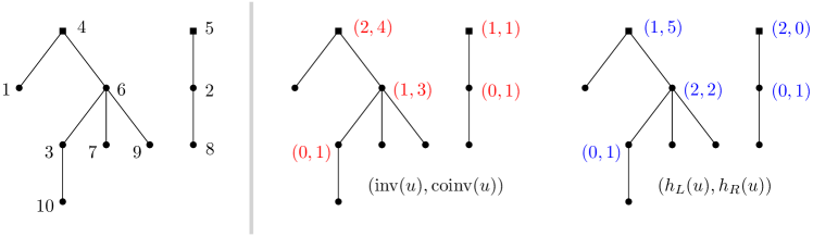
Figure 1. A forest $F\in\mathcal{R}_{10}$ (left) with $0pt(F)=14$, $\mathrm{inv}(F)=4$, $\mathrm{coinv}(F)=10$, $\mathrm{maj}(F)=5$ and $\mathrm{comaj}(F)=9$. Statistics $(\mathrm{inv}(u),\mathrm{coinv}(u))$ and $(h_{L}(u),h_{R}(u))$ are shown beside non-leaf vertices $u$ in red and blue (right).

The inversion/major indices on forests are generalizations of well-known Mahonian statistics on $\mathfrak{S}_{n}$ of the same name. The extensions of $\mathrm{inv}(\cdot)$ and $\mathrm{maj}(\cdot)$ from $\mathfrak{S}_{n}$ to $\mathcal{R}_{n}$ are due to Mallows and Riordan [MR68] and Björner and Wachs [BW89], respectively.

Note that $\mathrm{inv}(F)$ and $\mathrm{coinv}(F)$ are equidistributed over $\mathcal{R}_{n}$, as can be seen by exchanging vertex labels $i$ and $n+1-i$. The same is true of $\mathrm{maj}(F)$ and $\mathrm{comaj}(F)$. Our interest lies in the joint distributions $(\mathrm{inv},\mathrm{coinv})$ and $(\mathrm{maj},\mathrm{comaj})$, which turn out to coincide over $\mathcal{R}_{n}$ just as they do over $\mathfrak{S}_{n}$. We will elaborate on the relationship between these statistics in Section 1.5.

Let $\mathcal{T}_{n}$ be the set of trees on vertices $[n]$. Note that removal of vertex 0 puts these trees in natural correspondence with rooted forests on $[1,n]$. While we have cast our work in terms of rooted forests, all statements regarding $\mathcal{R}_{n}$ can be translated mutatis mutandis to the language of trees.

1.2. Factorizations of Full Cycles

It is well known that every $r$-cycle $\sigma\in\mathfrak{S}_{[n]}$ can be expressed as a product of $r-1$ transpositions but no fewer. Accordingly, a sequence $(\tau_{1},\ldots,\tau_{r-1})$ of transpositions satisfying $\sigma=\tau_{1}\tau_{2}\cdots\tau_{r-1}$ is called a minimal factorization of $\sigma$. For example, the canonical decompositions

(1) $$(a_{0}\,a_{1})(a_{0}\,a_{2})\cdots(a_{0}\,a_{r})$$

and

(2) $$(a_{0}\,a_{r})(a_{1}\,a_{r})\cdots(a_{r-1}\,a_{r})$$

are minimal factorizations of $\sigma=(a_{0}\,a_{1}\,\cdots\,a_{r})$. These will play a central role in our analysis and we refer to them as the lower and upper decompositions of $\sigma$, respectively.

Let $\mathcal{F}_{n}$ be the set of minimal factorizations of the full cycle $\sigma_{n}=(0\,1\,2\,\cdots\,n)$. For example

$$\mathcal{F}_{1} =\{(0\;1)\},$$

$$\mathcal{F}_{2} =\{(0\;1)(0\;2),(0\;2)(1\;2),(1\;2)(0\;1)\}.$$

Minimal factorizations of a fixed full cycle have long been known to be related to labelled trees (equivalently, rooted forests). The identity $|\mathcal{F}_{n}|=(n+1)^{n-1}=|\mathcal{R}_{n}|$ dates back at least to Hurwitz but is often credited to Dénes [Dé59], who offered an elegant proof via indirect counting. Direct bijections between $\mathcal{F}_{n}$ and $\mathcal{R}_{n}$ came later. The simplest of these, due to Moszkowski [Mos89], has been rediscovered in different guises by a number of authors. Its essence is the fact that trees are a special class of planar maps, and minimal factorizations (broadly speaking) serve as combinatorial encodings of planar embeddings. A version of this bijection is central to our construction and described in Section 2.1.

The connection between $\mathcal{R}_{n}$ and $\mathcal{F}_{n}$ can be refined to account for forest inversions/coinversions. The corresponding statistics for factorizations, which we call area and coarea, are defined for $f=(a_{1}\,b_{1})(a_{2}\,b_{2})\cdots(a_{n}\,b_{n})\in\mathcal{F}_{n}$ by

$$\mathrm{area}(f)=\binom{n}{2}-\sum_{i=1}^{n}a_{i}\qquad\textnormal{ and }\qquad\mathrm{coarea}(f)=\sum_{i=1}^{n}(b_{i}-1)-\binom{n}{2}.$$

With this terminology the main result of our previous paper [IR21] can be stated as follows.

Theorem 1.1.

For any $n\geq 0$, the bi-statistics $(\mathrm{inv},\mathrm{coinv})$ on $\mathcal{R}_{n}$ and $(\mathrm{area},\mathrm{coarea})$ on $\mathcal{F}_{n}$ share the same joint distribution.

Our proof of Theorem 1.1 relied on generating series techniques but was effectively based on a recursive bijection. In Section 2 we shall reestablish this result by describing a natural and direct bijection between $\mathcal{F}_{n}$ and $\mathcal{R}_{n}$ that maps $(\mathrm{area},\mathrm{coarea})$ to $(\mathrm{maj},\mathrm{comaj})$. This will serve as a base case toward extending Theorem 1.1 to treat factorizations into $(k+1)$-cycles for arbitrary $k\geq 1$.

1.3. Minimal $k$-Factorizations

For $k,n\geq 1$, let $\mathcal{F}_{n}^{k}$ be the set of all sequences $(\tau_{1},\ldots,\tau_{n})$ of $(k+1)$-cycles $\tau_{i}\in\mathfrak{S}_{[kn]}$ such that $\tau_{1}\tau_{2}\cdots\tau_{n}=\sigma_{kn}$. In particular, we have $\mathcal{F}_{n}^{1}=\mathcal{F}_{n}$.

Certainly $\mathcal{F}_{n}^{k}$ is nonempty, as taking $\tau_{i}=(0,in+1,in+2,\ldots,in)$ for $1\leq k\leq n$ defines one canonical element. Moreover, the cycle $\sigma_{kn}$ cannot be factored into fewer $(k+1)$-cycles, since replacing each factor with its lower expansion would then yield a factorization into fewer than $kn$ transpositions. As such we call the elements of $\mathcal{F}_{n}^{k}$ minimal $k$-factorizations of $\sigma_{kn}$, or simply $k$-factorizations for short.

Minimal $k$-factorizations of full cycles are well-studied and, unsurprisingly, they correspond with a class of decorated forests. These will be defined shortly, but in preparation for stating our main result, we first describe how the area/coarea statistics on $\mathcal{F}_{n}$ can be extended to $\mathcal{F}_{n}^{k}$.

Let

(3) $$f=(a_{1}^{0}\,\cdots\,a_{1}^{k})\cdots(a_{n}^{0}\,\cdots\,a_{n}^{k})$$

be a generic element of $\mathcal{F}_{n}^{k}$, keeping in mind our convention that $a_{i}^{0}$ is the least element of the $i$-th factor. Then we define

$$\begin{split}\mathrm{area}_{k}(f)&:=\binom{kn}{2}-n\binom{k}{2}-k\sum_{j=1}^{n}a^{0}_{j},\\ \mathrm{coarea}_{k}(f)&:=k\sum_{j=1}^{n}(a^{k}_{j}-1)-\binom{kn}{2}-n\binom{k}{2}.\end{split}$$

The careful reader may observe that these expressions share a common factor of $k$, e.g. $\mathrm{area}_{k}(f)=k\cdot(k\binom{n}{2}-\sum_{j}a_{j}^{0})$. This apparent redundancy will arise naturally in our analysis so we have chosen not to “normalize” it out of our definitions.

We further introduce two additional statistics on $\mathcal{F}_{n}^{k}$ that we call semiarea and cosemiarea, given by

$$\begin{split}\mathrm{semiarea}_{k}(f)&:=\binom{kn}{2}-\sum_{i=0}^{k-1}\sum_{j=1}^{n}a_{j}^{i},\\ \mathrm{cosemiarea}_{k}(f)&:=\sum_{i=1}^{k}\sum_{j=1}^{n}(a_{j}^{i}-1)-\binom{kn}{2}.\end{split}$$

Although not obvious from these definitions, it transpires that $\mathrm{semiarea}_{k}(f)$ and $\mathrm{cosemiarea}_{k}(f)$ are also always divisible by $k$. Note that both $\mathrm{area}_{k}(f)$ and $\mathrm{semiarea}_{k}(f)$ revert to $\mathrm{area}(f)$ at $k=1$, but are otherwise distinct. The same is true for coareas.

1.4. Rooted $k$-Forests

A $k$-forest is a rooted labelled forest $F$ equipped with a function $\kappa:E(F)\rightarrow[k-1]$ that assigns one of $k$ colours $\{0,1,\ldots,k-1\}$ to each edge of $F$. Two $k$-forests $(F,\kappa)$ and $(F^{\prime},\kappa^{\prime})$ are isomorphic if there is a graph isomorphism $\zeta\,:\,V(F)\rightarrow V(F^{\prime})$ that preserves roots and edge colours.

Let $\mathcal{R}_{n}^{k}$ be the set of $k$-forests on vertices $[1,n]$. Note that there are no restrictions on the colouring function, so there are $k^{|E(F)|}=k^{n-c}$ elements of $\mathcal{R}_{n}^{k}$ arising from any forest $F\in\mathcal{R}_{n}$ with $c$ components. For brevity we will suppress explicit mention of the colouring function when working with elements of $\mathcal{R}_{n}^{k}$.

Our definition of $k$-forests follows Yan [Yan97], who attributes them to Stanley. These objects appear elsewhere in the literature in the different but equivalent form of $k$-cacti, which are tree-like structures with edges replaced by $(k+1)$-gons. In particular, there is a simple correspondence between $k$-forests on $n$ labelled vertices and $k$-cacti with $n$ labelled polygons. See Figure 2.

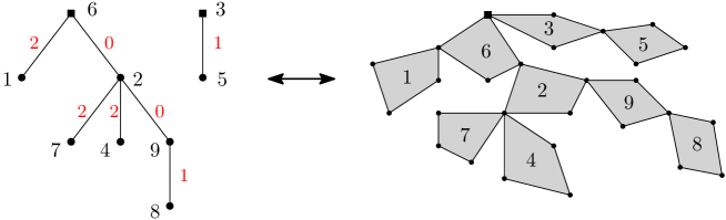
Figure 2. A $3$-forest $F$ and its associated $3$-cactus $C$. Vertices of of $F$ correspond with polygons of $C$. The colouring of $F$ is indicated in red. The colour of edge $(i,j)$ describes where $P_{j}$ (polygon $j$) is attached to $P_{i}$ in $C$. For example, edge $(9,8)$ with colour 1 indicates $P_{8}$ is attached to $P_{9}$ at the second vertex clockwise from where $P_{9}$ is attached to its parent, $P_{2}$.

A straightforward extension of the Prüfer encoding yields $|\mathcal{R}_{n}^{k}|=(kn+1)^{n-1}$, and the Moszkowski correspondence $\mathcal{F}_{n}\leftrightarrow\mathcal{R}_{n}$ likewise extends to a bijection between $\mathcal{F}_{n}^{k}$ and $\mathcal{R}_{n}^{k}$. In particular, we have $|\mathcal{F}_{n}^{k}|=(kn+1)^{n-1}$. We direct the reader to [Irv09] and references therein for further information, however all details relevant to our discussion will be outlined when required.

The Mahonian statistics $\mathrm{inv}/\mathrm{coinv}$ and $\mathrm{maj}/\mathrm{comaj}$ on $\mathcal{R}_{n}$ can be applied to $\mathcal{R}_{n}^{k}$ simply by ignoring edge colourings. However, we also wish to introduce extended versions of these statistics specifically for $k$-forests.

To this end we first define the chromatic depth and chromatic codepth of $F\in\mathcal{R}_{n}^{k}$ by

(4) $$\mathrm{chr}_{k}(F)=\sum_{e=(u,v)\in E(F)}\kappa(e)\cdot h(v)\;\;\;\textnormal{and}\;\;\;{\mathrm{cochr}}_{k}(F)=\sum_{e=(u,v)\in E(F)}(k-1-\kappa(e))\cdot h(v),$$

respectively. Note that $\mathrm{chr}_{k}(F)=0pt(F)$ when $F$ has all its edges coloured 1, so $\mathrm{chr}_{k}(F)$ can be regarded as a colour-weighted depth of $F$. We then let

$$\begin{split}\mathrm{inv}_{k}(F)&:=\mathrm{inv}(F)+\mathrm{chr}_{k}(F),\\ \mathrm{coinv}_{k}(F)&:=\mathrm{coinv}(F)+{\mathrm{cochr}}_{k}(F),\end{split}$$

and

$$\begin{split}\mathrm{maj}_{k}(F)&:=\mathrm{maj}(F)+\mathrm{chr}_{k}(F),\\ \mathrm{comaj}_{k}(F)&:=\mathrm{comaj}(F)+{\mathrm{cochr}}_{k}(F).\end{split}$$

These extended statistics revert to $\mathrm{inv}/\mathrm{maj}$ at $k=1$ since $\mathrm{chr}_{1}(F)={\mathrm{cochr}}_{1}(F)=0$ for all $F\in\mathcal{R}_{n}$.

This definition of $\mathrm{inv}_{k}(F)$ is equivalent to that appearing in [Yan97], where it arose in an effort to generalize Kreweras’ identity between the inversion enumerator for trees and the discrepancy enumerator for parking functions (see [Kre80]). This connection will be discussed in more detail in Section 1.6. Consideration of $\mathrm{maj}_{k}(F)$ appears to be novel. It is straightforward (using Figure 2 as a guide) to adapt the definitions of $\mathrm{inv}_{k},\mathrm{coinv}_{k},\mathrm{maj}_{k},$ and $\mathrm{comaj}_{k}$ so they apply to $k$-cacti.

1.5. Main Result

We can now state our main theorem, which relates area statistics on $k$-factorizations to major indices on $k$-forests.

Theorem 1.2.

For any $n,k\geq 1$, there is an explicit bijection $\phi:\mathcal{F}_{n}^{k}\rightarrow\mathcal{R}_{n}^{k}$ such that for $F=\phi(f)$ we have

$$\mathrm{area}_{k}(f) =k\cdot\mathrm{maj}_{k}(F), \mathrm{coarea}_{k}(f) =k\cdot\mathrm{comaj}_{k}(F)$$

and

$$\mathrm{semiarea}_{k}(f) =k\cdot\mathrm{maj}(F), \mathrm{cosemiarea}_{k}(f) =k\cdot\mathrm{comaj}(F).$$

Moreover, if $f=(a_{1}^{0}\,\cdots\,a_{1}^{k})\cdots(a_{n}^{0}\,\cdots\,a_{n}^{k})$ then $a_{i}^{k}-a_{i}^{0}=k\cdot h(i)$ for $i\in[1,n]$, where $h(i)$ is the hook length at vertex $i$ in $F$.

Theorem 1.2 will be proved first for $k=1$ in Section 2 and then in general in Section 3. In each case the proof is through construction of the promised bijection $\phi$. Note that the theorem implies $\mathrm{semiarea}_{k}(f)$ and $\mathrm{cosemiarea}_{k}(f)$ are independent of the edge colouring of $F=\phi(f)$. The edge colours of $F$ are only relevant to the evaluation of $\mathrm{area}_{k}(f)$ and $\mathrm{coarea}_{k}(f)$.

We will now describe precisely how Theorem 1.2 can be viewed as a generalization of Theorem 1.1. The key is that $\mathrm{maj}(F)$ and $\mathrm{inv}(F)$ are equidistributed not only over $\mathcal{R}_{n}$, but over every isomorphism class thereof. This was first proved inductively by Björner and Wachs [BW89], and later bijectively by Liang and Wachs [LW92]. More recently, Grady and Poznanović [GP16] established this result by mapping both $\mathrm{inv}(F)$ and $\mathrm{maj}(F)$ to a common code called a subexcedant sequence on $F$. We will not go into further detail here. The salient point is that there are known bijections $\xi\,:\,\mathcal{R}_{n}\rightarrow\mathcal{R}_{n}$ satisfying $\mathrm{maj}(F)=\mathrm{inv}(\xi(F))$ with $F$ isomorphic to $\xi(F)$ for all $F\in\mathcal{R}_{n}$. For definiteness, let gp be the Grady-Poznanović bijection of this type.

Note that gp extends to a bijection on $\mathcal{R}_{n}^{k}$ by effectively ignoring edge colours. Let $F\in\mathcal{R}_{n}^{k}$ and $F^{\prime}={\textsc{gp}}(F)$, so that $F$ and $F^{\prime}$ are isomorphic as $k$-forests and $\mathrm{maj}(F)=\mathrm{inv}(F^{\prime})$. Then

$$0pt(F)=0pt(F^{\prime}) \implies\mathrm{maj}(F)+\mathrm{comaj}(F)=\mathrm{inv}(F^{\prime})+\mathrm{coinv}(F^{\prime})$$

$$\implies\mathrm{comaj}(F)=\mathrm{coinv}(F^{\prime}).$$

It is clear from (4) that chromatic depth and codepth are invariant on isomorphism classes of $\mathcal{R}_{n}^{k}$, so there follows $\mathrm{maj}_{k}(F)=\mathrm{inv}_{k}(F^{\prime})$ and $\mathrm{comaj}_{k}(F)=\mathrm{coinv}_{k}(F^{\prime})$.

Let $\phi:\mathcal{F}_{n}^{k}\rightarrow\mathcal{R}_{n}^{k}$ be the bijection guaranteed by Theorem 1.2. Then taking $\hat{\phi}={\textsc{gp}}\circ\phi$ proves the following generalization of Theorem 1.1. We shall see in the next section how this sheds light on an open question concerning the relationship between $k$-forests and generalized parking functions.

Corollary 1.3.

For any $n,k\geq 1$, there is an explicit bijection $\hat{\phi}:\mathcal{F}_{n}^{k}\rightarrow\mathcal{R}_{n}^{k}$ such that for $F=\hat{\phi}(f)$ we have $(\mathrm{area}_{k}(f),\mathrm{coarea}_{k}(f))=k\cdot(\mathrm{inv}_{k}(F),\mathrm{coinv}_{k}(F))$ and $(\mathrm{semiarea}_{k}(f),\mathrm{cosemiarea}_{k}(f))=k\cdot(\mathrm{inv}(F),\mathrm{coinv}(F))$.

Let us now consider the latter claim of Theorem 1.2, regarding hook lengths. In case $k=1$ the theorem stipulates that the distribution of the hook length vector $(h(1),\ldots,h(n))$ over $F\in\mathcal{R}_{n}$ matches that of the difference index $(b_{1}-a_{1},\cdots,b_{n}-a_{n})$ over $f=(a_{1}\,b_{1})\cdots(a_{n}\,b_{n})\in\mathcal{F}_{n}$. A similar result appears in [GY02], although there the authors compute transposition differences circularly, replacing $b-a$ with $\min\{b-a,n+1+a-b\}$. This has the effect of disguising the connection with hook lengths, despite the use of a dual construction equivalent to that used here (see Section 2.2).

Over the past couple decades, a considerable amount of effort has been put toward the development of hook length formulae for trees and forests. These formulae generally provide simple multiplicative expressions for sums of the form $\sum_{T\in\mathcal{T}}\prod_{v\in V(T)}\alpha(v)$, where $\mathcal{T}$ is a class of rooted trees and $\alpha(v)$ can be expressed in terms of the hook length of $T$ at $v$.

For the class of rooted labelled forests, one of the simplest such formulae is

(5) $$\sum_{F\in\mathcal{R}_{n}}z^{c(F)}\prod_{v\in V(F)}\frac{1}{h(v)}=z(z+1)(z+2)\cdots(z+n-1),$$

where $c(F)$ is the number of components in $F$. This reflects the fact that permutations on $[1,n]$ with $m$ cycles — which are well known to be counted by the coefficient of $z^{m}$ on the right-hand side, i.e. the signless Stirling number $s(n,m)$ — are in correspondence with increasing rooted forests on $[1,n]$ with $m$ components. See [GS06] for a more general approach, in particular Corollary 6.3, of which (5) is a special case.

Using (5) at $z=1$ together with Theorem 1.2 at $k=1$ yields the curious identity

$$\sum_{f\in\mathcal{F}_{n}}\prod_{i=1}^{n}\frac{1}{b_{i}-a_{i}}=n!,$$

where the sum extends over all factorizations $f=(a_{1}\,b_{1})\cdots(a_{n}\,b_{n})\in\mathcal{F}_{n}$. More generally, since there are $k^{n-c(F)}$ ways of colouring a forest $F\in\mathcal{R}_{n}$ to create a $k$-forest $F^{\prime}\in\mathcal{R}_{n}^{k}$, we can apply (5) at $z=1/k$ to get:

Corollary 1.4.

For any $n,k\geq 1$, we have

$$\sum_{f\in\mathcal{F}_{n}^{k}}\prod_{i=1}^{n}\frac{1}{a_{i}^{k}-a_{i}^{0}}=\frac{(k+1)(2k+1)\cdots((n-1)k+1)}{k^{n}},$$

where the sum extends over all $f=(a_{1}^{0}\,\cdots\,a_{1}^{k})\cdots(a_{n}^{0}\,\cdots\,a_{n}^{k})\in\mathcal{F}_{n}^{k}$.

1.6. $k$-Parking Functions

A sequence $p=(a_{1},\dots,a_{n})$ of nonnegative integers is called a $k$-parking function if its nondecreasing rearrangement $(b_{1},\dots,b_{n})$ satisfies $b_{i}\leq k(i-1)$ for $1\leq i\leq n$. Let $\mathcal{P}_{n}^{k}$ be the set of $k$-parking functions of length $n$. Elements of $\mathcal{P}_{n}:=\mathcal{P}_{n}^{1}$ are simply called parking functions. There is an extensive body of literature on these object and we will only skim the surface here. We refer the reader to the comprehensive surveys by Yan [Yan15] and Haglund [Hag08] for further information.

It is well known, and easy to prove via cycle lemma or direct bijection, that $|\mathcal{P}_{n}^{k}|=|\mathcal{R}_{n}^{k}|=(kn+1)^{n-1}$. This can be refined to account for inversions in $k$-forests. The companion statistic on $k$-parking functions is called displacement, defined for $p=(a_{1},\ldots,a_{n})\in\mathcal{P}_{n}^{k}$ by

(6) $$\mathrm{disp}_{k}(p):=k\binom{n}{2}-\sum_{i=1}^{n}a_{i}.$$

Then we have the following result, which was first proved for $k=1$ by Kreweras [Kre80] and then for general $k\geq 1$ by Yan.

Theorem 1.5 ([Yan97]).

For $n,k\geq 1$

$$\sum_{p\in\mathcal{P}_{n}^{k}}q^{\mathrm{disp}_{k}(p)}=\sum_{F\in\mathcal{R}_{n}^{k}}q^{\mathrm{inv}_{k}(F)}.$$

Yan’s proof of Theorem 1.5 is inductive, and it has been an open problem to find a bijective proof. Such a proof is afforded by Corollary 1.3 in tandem with the simple correspondence between $\mathcal{F}_{n}^{k}$ and $\mathcal{P}_{n}^{k}$ described below.

Proposition 1.6.

For fixed $n,k\geq 1$, define $L\,:\,\mathcal{F}_{n}^{k}\rightarrow[kn]^{n}$ by

$$L:(a_{1}^{0}\,\cdots\,a_{1}^{k})\cdots(a_{n}^{0}\,\cdots\,a_{n}^{k})\mapsto(a_{1}^{0},\dots,a_{n}^{0}).$$

Then $L$ is a bijection from $\mathcal{F}_{n}^{k}$ to $\mathcal{P}_{n}^{k}$, and $\mathrm{area}_{k}(f)=k\cdot\mathrm{disp}_{k}(L(f))$ for all $f$.

Assuming the truth of the proposition, and letting $\hat{\phi}\,:\,\mathcal{F}_{n}^{k}\rightarrow\mathcal{R}_{n}^{k}$ be the bijection from Corollary 1.3, observe that $L\circ\hat{\phi}^{-1}$ maps $\mathcal{R}_{n}^{k}$ bijectively to $\mathcal{P}_{n}^{k}$ while satisfying $\mathrm{inv}_{k}(F)=\frac{1}{k}\cdot\mathrm{area}_{k}(\hat{\phi}^{-1}(f))=\mathrm{disp}_{k}(L(\hat{\phi}^{-1}(F)))$. This is the promised bijective proof of Theorem 1.5.

The latter claim of Proposition 1.6 is an immediate consequence of the definitions. The bijectivity of ${L}:{\mathcal{F}_{n}^{k}}\rightarrow{\mathcal{P}_{n}^{k}}$ when $k=1$ was proved explicitly by Biane [Bia02] and is equivalent to an earlier result of Stanley [Sta97, Theorem 3.1]. We call this special case of $L$ the Stanley-Biane bijection, denoted ${\textsc{sb}}:\mathcal{F}_{n}\rightarrow\mathcal{P}_{n}$. A proof of bijectivity for general $k$ recently appeared in [MNW20], where it was established through a straightforward generalization of Biane’s argument. We will now describe a different (independent) proof that relies on a reduction to sb.

Consider the function ${\textsc{expand}}:\mathcal{P}_{n}^{k}\rightarrow\mathcal{P}_{kn}$ that replaces each entry of a $k$-parking function with $k$ copies of itself. For instance, $p=(0,5,1)\in\mathcal{P}_{3}^{3}$ has ${\textsc{expand}}(p)=(0,0,0,5,5,5,1,1,1)\in\mathcal{P}_{9}$.

Similarly define the function ${\textsc{lower}}:\mathcal{F}_{n}^{k}\rightarrow\mathcal{F}_{kn}$ that replaces each cyclic factor of a $k$-factorization with its lower decomposition; see (1). For example, $f=(1\,2\,5)(0\,1\,6)(3\,4\,5)\in\mathcal{F}_{3}^{2}$ has ${\textsc{lower}}(f)=(1\,2)(1\,5)(0\,1)(0\,6)(3\,4)(3\,5)\in\mathcal{F}_{6}$.

Certainly both expand and lower are injective for all $k$ (although not bijective for $k>1$). It is also clear that ${\textsc{sb}}\circ{\textsc{lower}}(\mathcal{F}_{n}^{k})\subseteq{\textsc{expand}}(\mathcal{P}_{n}^{k})$. Thus ${\textsc{expand}}^{-1}\circ{\textsc{sb}}\circ{\textsc{lower}}$ is a well-defined injective function from $\mathcal{F}_{n}^{k}$ to $\mathcal{P}_{n}^{k}$, and by definition it agrees with $L$ on its domain. Since $|\mathcal{F}_{n}^{k}|=|\mathcal{P}_{n}^{k}|$, we conclude that $L$ is bijective.

Finally, a comment on nomenclature. It is common to view a $k$-parking function $p=(a_{1},\ldots,a_{n})\in\mathcal{P}_{n}^{k}$ as a specially labelled lattice path from $(0,0)$ to $(n,kn)$, with unit steps to the north and east, that remains weakly below the line $y=kx$. For each $h\in[kn-1]$ let $I_{h}=\{i:a_{i}=h\}$. Then the path $P$ corresponding to $p$ has $|I_{h}|$ horizontal steps at height $h$ and these are labelled in increasing left-right order with the set $I_{h}$. The displacement $\mathrm{disp}_{k}(p)$ is then the number of whole squares between $P$ and the line $y=kx$. For this reason, $\mathrm{disp}_{k}(p)$ is also known as the area of $p$. In light of Proposition 1.6, this explains our naming of the statistics $\mathrm{area}_{k}/\mathrm{coarea}_{k}$ on $\mathcal{F}_{n}^{k}$.

2. The construction for $k=1$

In this section we focus on the case $k=1$ of Theorem 1.2. The bijection ${\phi}:{\mathcal{F}_{n}}\rightarrow{\mathcal{R}_{n}}$ that we construct in this case has a particularly simple description and will be central to our analysis for general $k$. Throughout we shall simplify our notation by omitting the value of $k$, using $\mathcal{R}_{n}$ in place of $\mathcal{R}_{n}^{1}$, $\mathrm{area}(f)$ for $\mathrm{area}_{1}(f)$, etc.

2.1. Arch Diagrams

Let $\mathcal{E}_{n}$ be the set of vertex-rooted, edge-labelled trees on $n$ edges, by which we mean trees with a distinguished vertex whose edges are distinctly labelled with $[1,n]$. Vertices are not labelled.

We typically will not distinguish between an edge and its label; i.e. we view $[1,n]$ as the edge-set of any tree $T\in\mathcal{E}_{n}$. As with rooted forests, we regard the edges of these trees as being directed away from the root. It will be convenient to let $d(i)$ denote the child (‘down’) endpoint of edge $i$.

There is a simple correspondence between $\mathcal{E}_{n}$ and $\mathcal{R}_{n}$, defined as follows: Given $T\in\mathcal{E}_{n}$, we first ‘push’ the label of each edge $i$ away from the root onto vertex $d(i)$, and then remove the root to obtain a rooted forest $F\in\mathcal{R}_{n}$. We call this the Cayley bijection, written ${\textsc{cay}}\,:\,\mathcal{E}_{n}\rightarrow\mathcal{R}_{n}$. See Figure 3.

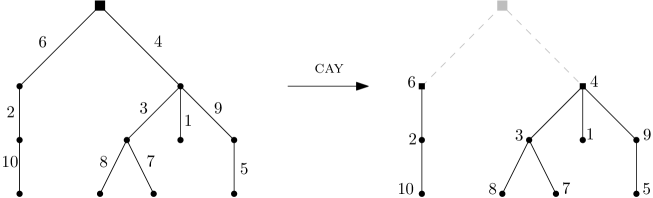
Figure 3. A vertex-rooted, edge-labelled tree $T\in\mathcal{E}_{10}$ (left) and its image ${\textsc{cay}}(T)\in\mathcal{R}_{10}$ (right). The boxed vertices indicate roots. The major index of both $T$ and ${\textsc{cay}}(T)$ is 7 and their comajor index is 5.

Our interest in edge-labelled trees stems from the fact that they are in natural correspondence with factorizations of full cycles.

Consider a planar embedding of $T\in\mathcal{E}_{n}$ described as follows:

1. the root is at $(0,0)$, and all other vertices at $(i,0)$ for $1\leq i\leq n$;

2. edges are labelled $[1,n]$ and are drawn above the $x$-axis without crossings; and

3. the sequence of edge labels around each vertex, taken in counterclockwise order beginning on the $x$-axis, is increasing.

Following [IR21], we call an embedding of a member of $\mathcal{E}_{n}$ satisfying (1)–(3) an arch diagram of size $n$. Let $\mathcal{A}_{n}$ be set of all such diagrams up to topological equivalence. The embedding process described above provides a one-one correspondence $\mathcal{E}_{n}\leftrightarrow\mathcal{A}_{n}$.

We canonically label the vertices of each diagram $A\in\mathcal{A}_{n}$ by assigning label $i$ to the vertex at $(i,0)$, for $0\leq i\leq n$. We emphasize that these labels are completely determined by $A$ itself, or equally by its skeletal tree $T\in\mathcal{E}_{n}$. We then obtain from $A$ a factorization $f=(a_{1}\,b_{1})(a_{2}\,b_{2})\cdots(a_{n}\,b_{n})\in\mathcal{F}_{n}$ by letting $a_{i}$ and $b_{i}$ be the endpoints of arch $i$. See Figure 4.

Figure 4. The arch diagram $A\in\mathcal{A}_{10}$ corresponding to the factorization $f=(6\,7)(0\,2)(3\,6)(3\,10)(8\,9)(0\,3)(5\,6)(4\,5)(8\,10)(1\,2)\in\mathcal{F}_{10}$. Vertices are canonically labelled.

The transformation $A\mapsto f$ turns out to be a bijection from $\mathcal{A}_{n}$ to $\mathcal{F}_{n}$. We denote this function by ${{\textsc{fact}}}:{\mathcal{A}_{n}}\rightarrow{\mathcal{F}_{n}}$ and its inverse by ${{\textsc{arch}}}:{\mathcal{F}_{n}}\rightarrow{\mathcal{A}_{n}}$. The direct definition of arch is obvious: Given $f=(a_{1}\,b_{1})\cdots(a_{n}\,b_{n})\in\mathcal{F}_{n}$, construct ${\textsc{arch}}(f)$ by drawing an arch labelled $i$ from $(a_{i},0)$ to $(b_{i},0)$ for each $1\leq i\leq n$. See [IR21] for a more detailed description of these transformations based on the ‘circle-chord’ construction from [GY02]. The composite mapping ${\textsc{fact}}\circ{\textsc{cay}}^{-1}$ is essentially a repackaging of Moszkowski’s bijection $\mathcal{R}_{n}\rightarrow\mathcal{F}_{n}$ referenced in Section 1.2.

Let $A$ be a fixed arch diagram. We write $l(i)$ and $r(i)$, respectively, for the left and right endpoints of edge $i$ in $A$, and we define its span to be the half open interval $\mathrm{span}(i):=\{(x,0):x\in[l(i),r(i))\}$. Since distinct edges cannot cross, their spans are either disjoint or one is contained in the other. Thus the edges of $A$ are partially ordered by inclusion of their spans. We say $j$ covers $i$ if $\mathrm{span}(i)\subset\mathrm{span}(j)$ and there is no arch $\ell$ with $\mathrm{span}(i)\subsetneq\mathrm{span}(\ell)\subsetneq\mathrm{span}(j)$.

2.2. Dual Diagrams

An arch diagram $A\in\mathcal{A}_{n}$ divides the upper half-plane $\{(x,y)\,:\,y\geq 0\}$ into $n+1$ regions, each of which contains exactly one point from the set $H_{n}=\{(i+\frac{1}{2},0):0\leq i\leq n\}$. Each arch separates two regions and hence two points of $H_{n}$. We construct a planar dual $D$ of $A$ by first placing a vertex at each point of $H_{n}$ and then, for each $i\in[1,n]$, drawing an arch labelled $\bar{i}$ between the two points of $H_{n}$ that are separated by arch $i$ of $A$. See Figure 5. Note our use of overlined symbols $\bar{1},\bar{2},\ldots,\bar{n}$ for edge labels in the dual. This notational convention will be used systematically to distinguish labels in $D$ from those in $A$.

So constructed, the dual of any arch diagram $A\in\mathcal{A}_{n}$ is an embedding of a tree $T\in\mathcal{E}_{n}$ satisfying the following:

1. vertices lie at the points $H_{n}$, with the root at $(n+\frac{1}{2},0)$;

2. edges are labelled $[\bar{1},\bar{n}]$ and are drawn above the $x$-axis without crossings; and

3. the sequence of edge labels around each vertex, taken in counterclockwise order beginning on the $x$-axis, is decreasing.

Let $\mathcal{D}_{n}$ be set of topologically inequivalent embeddings satisfying $(1^{\prime})-(3^{\prime})$. Clearly the map ${{\textsc{dual}}}:{\mathcal{A}_{n}}\rightarrow{\mathcal{D}_{n}}$ described above is a bijection. We call elements of $\mathcal{D}_{n}$ dual diagrams of size $n$ and canonically label their vertices by assigning label $i$ to the vertex at $(i+\tfrac{1}{2},0)$ for $0\leq i\leq n$.

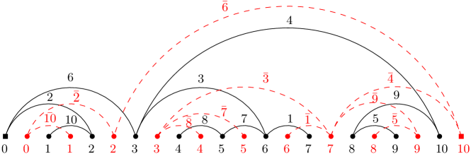
Figure 5. The arch diagram $A\in\mathcal{A}_{10}$ of Figure 4 in drawn in black and its dual $D\in\mathcal{D}_{10}$ in dashed red. The skeletal tree $T\in\mathcal{E}_{10}$ of $D$ is displayed in Figure 3 along with its corresponding forest $F\in\mathcal{R}_{10}$.

The transparent bijection between dual diagrams and their skeletal trees allows us to identify $\mathcal{D}_{n}$ and $\mathcal{E}_{n}$. In particular, we shall view the Cayley bijection as a correspondence between $\mathcal{D}_{n}$ and $\mathcal{F}_{n}$. Note that ${\textsc{cay}}({\textsc{dual}}(A))$ is the Hasse diagram of the poset of edges of $A$ (ordered by inclusion). Compare, for instance, Figures 3 and 4.

Lemma 2.1.

Let $f=(a_{1},\,b_{1})\cdots(a_{n}\,b_{n})\in\mathcal{F}_{n}$, $A={\textsc{arch}}(f)$, $D={\textsc{dual}}(A)$ and $F={\textsc{cay}}(D)$. For each $i\in[1,n-1]$, the following are equivalent:

1. $a_{i}=a_{i+1}$

2. edge $i+1$ covers edge $i$ in $A$

3. edge $\overline{i}$ is incident with vertex $d(\overline{i+1})$ in $D$

4. vertex $i$ is a child of vertex $i+1$ in $F$

Proof.

Condition (1) is equivalent to $l(i)=l(i+1)$ in $A$ (by definition of arch), and the requirement that edge labels increase counterclockwise around vertex $l(i)$ makes this equivalent to (2). The equivalences $(2)\iff(3)\iff(4)$ follow by definition of dual and cay. ∎

2.3. Proof of Theorem 1.2 (Base Case)

Lemma 2.2.

Let $A\in\mathcal{A}_{n},D={\textsc{dual}}(A)$ and $F={\textsc{cay}}(D)$. Then for $i\in[1,n]$ we have $h(i)=r(i)-l(i)$, where $i$ specifies a vertex of $F$ on the left-hand side and an edge of $A$ on the right. More precisely, we have

$$h_{L}(i)=d(\bar{i})-l(i)\qquad\text{and}\qquad h_{R}(i)=r(i)-d(\bar{i})-1.$$

Proof.

We refer the reader to Figure 6, which illustrates a portion of $A$ in solid black and $D$ in dashed red.

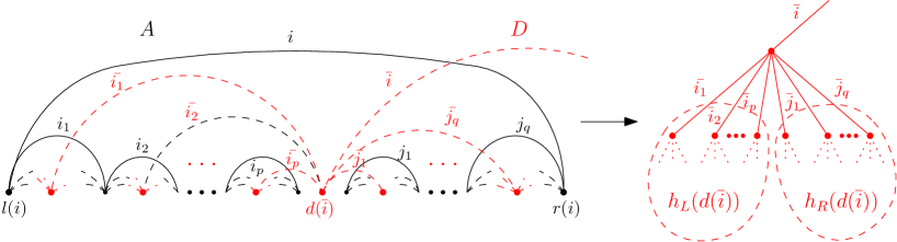
Figure 6. A portion of an arch diagram $A$ (black) and its dual $D$ (red).

Consider edge $i$ of $A$. By construction, only one dual edge may cross this arch, namely $\bar{i}$. Thus the vertices of $D$ lying within $\mathrm{span}(i)$ are precisely those in the dual hook $H(d(\bar{i}))$. Clearly there are $r(i)-l(i)$ dual vertices in $\mathrm{span}(i)$, so we have $h(i)=r(i)-l(i)$.

Let $\bar{j}_{1}>\cdots>\bar{j}_{q}>i>\bar{i}_{1}>\cdots>\bar{i}_{p}$ be the edges of $D$ incident with $d(\bar{i})$. Since edge labels must decrease counterclockwise around $d(\bar{i})$, and since edges may not cross, all vertices of $H(d(\bar{i}_{1})),\ldots,H(d(\bar{i}_{p}))$ must lie to the left of $d(\bar{i})$, while those of $H(d(\bar{j}_{1})),\ldots,H(d(\bar{j}_{q}))$ lie to the right. There are $d(\bar{i})-l(i)$ dual vertices in $\mathrm{span}(i)$ to the left of $d(\bar{i})$, and $r(i)-d(\bar{i})-1$ to the right. Thus $d(\bar{i})-l(i)=\sum_{s=1}^{p}h(d(\bar{i}_{s}))$, and this is precisely the left hook length $h_{L}(i)$ in $F$. The expression for $h_{R}(i)$ follows since $h(i)=h_{L}(i)+h_{R}(i)+1$. ∎

Example 2.3.

In Figure 5, we have $d(\bar{4})=7$ and hook $H(7)$ of $D$ contains all dual (red) vertices lying within $\mathrm{span}(4)$, namely $\{3,4,\ldots,9\}$. Those to the left of $7$ contribute to $h_{L}(4)$ and those to the right contribute to $h_{R}(4)$. There are $d(\bar{4})-l(4)=7-3=4$ to the left and $r(4)-d(\bar{4})-1=10-7-1=2$ to the right. ∎

For fixed $n\geq 1$, let cda denote the composite map ${\textsc{cay}}\circ{\textsc{dual}}\circ{\textsc{arch}}:\mathcal{F}_{n}\rightarrow\mathcal{R}_{n}$, where again cay is interpreted to act on the skeletal trees of dual diagrams. We now show that this bijection satisfies the conditions described by Theorem 1.2, thus proving the theorem in the case $k=1$. (Recall that $\mathrm{(co)semiarea}_{k}$ coincides with $\mathrm{(co)area}$ in this case.)

Theorem 2.4.

The map ${\textsc{cda}}:\mathcal{F}_{n}\rightarrow\mathcal{R}_{n}$ is a bijection, and for $F={\textsc{cda}}(f)$ we have $\mathrm{area}(f)=\mathrm{maj}(F)$ and $\mathrm{coarea}(f)=\mathrm{comaj}(F)$. Moreover, if $f=(a_{1}\,b_{1})\cdots(a_{n}\,b_{n})$ then $h(i)=a_{i}-b_{i}$ for $1\leq i\leq n$, where $h(i)$ is the hook length at vertex $i$ in $F$.

Proof.

We have already seen that ${\textsc{cda}}\,:\,\mathcal{F}_{n}\rightarrow\mathcal{R}_{n}$ is a bijection.

Let $f=(a_{1}\,b_{1})\cdots(a_{n}\,b_{n})\in\mathcal{F}_{n}$, $A={\textsc{arch}}(f)$ and $D={\textsc{dual}}(A)$. By construction we have $l(i)=a_{i}$ and $r(i)=b_{i}$ for each arch $i$ of $A$, so Lemma 2.2 gives $h(i)=b_{i}-a_{i}$ for all $i$. Note that every non-root vertex of $D$ is the endpoint $d(\bar{i})$ of a unique edge $\bar{i}$. Thus $\{d(\bar{1}),\ldots,d(\bar{n})\}$ is a rearrangement of $\{0,\ldots,n-1\}$. With Lemma 2.2 we find that

$$\mathrm{maj}(F)=\sum_{i\in[1,n]}h_{L}(i)=\sum_{i\in[1,n]}(d(\bar{i})-l(i))=\binom{n}{2}-\sum_{i=1}^{n}a_{i}=\mathrm{area}(f).$$

The proof that $\mathrm{coarea}(f)=\mathrm{comaj}(D)$ is similar. ∎

Example 2.5.

We return to Figure 5, which shows $A={\textsc{arch}}(f)$ and $D={\textsc{dual}}(A)$ for the factorization $f=(a_{1}\,b_{1})\cdots(a_{10}\,b_{10})$ given by

$$(6\,7)(0\,2)(3\,6)(3\,10)(8\,9)(0\,3)(5\,6)(4\,5)(8\,10)(1\,2).$$

Note $(a_{4}\,b_{4})=(3\,\,10)$ and $h(d(\bar{4}))=7=a_{4}-b_{4}$. We have $\mathrm{area}(f)=\binom{10}{2}-\sum a_{i}=7$ and $\mathrm{coarea}(f)=\sum(b_{i}-1)-\binom{10}{2}=5$. The skeletal tree of $D$ is shown in Figure 3 along with its image $F$ under cay. We find that $\mathrm{maj}(F)=7$ and $\mathrm{comaj}(F)=5$, in agreement with Theorem 2.4. ∎

3. The main bijection for general $k$

In this section we prove Theorem 1.2 in the general case, building on the constructions used to prove Theorem 2.4.

Geometrically, our bijection from $\mathcal{F}_{n}^{k}$ to $\mathcal{R}_{n}^{k}$ is a natural extension of the map cda described in Section 2. Whereas factorizations $f\in\mathcal{F}_{n}$ correspond with planar embeddings of edge-labelled trees on $n$ edges (i.e. arch diagrams), $k$-factorizations $f\in\mathcal{F}_{n}^{k}$ correspond with embeddings of $k$-cacti having $n$ labelled polygons. We call such configurations generalized arch diagrams. Duals can be constructed analogously to the case $k=1$, and the skeletal $k$-cacti of the duals then correspond with a $k$-forests $F\in\mathcal{R}_{n}^{k}$ as described in Section 1.4. This generalized mapping $f\mapsto F$ is illustrated in Figure 7.

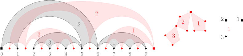
Figure 7. At left, the generalized arch diagram corresponding to the $3$-factorization $f=(6\,7\,8\,9)(0\,1\,5\,6)(2\,3\,4\,5)$ is shaded grey and its dual is shaded red. The skeletal $3$-cactus of the dual and its corresponding 3-forest are shown to the right.

Describing this simple geometrical transformation in sufficient detail to properly track statistics proves somewhat cumbersome. For the purposes of bookkeeping, we shall instead define this same mapping as a chain $\mathcal{F}_{n}^{k}\rightarrow\mathcal{F}_{kn}\rightarrow\mathcal{R}_{kn}\rightarrow\mathcal{R}_{n}^{k}$ having the bijection ${\textsc{cda}}:\,\mathcal{F}_{kn}\rightarrow\mathcal{R}_{kn}$ at its core. This allows direct use of Theorem 2.4.

3.1. Defining the Bijection

Recall from Section 1.6 the function ${\textsc{lower}}:\mathcal{F}_{n}^{k}\rightarrow\mathcal{F}_{kn}$ that replaces each factor of $f\in\mathcal{F}_{n}^{k}$ with its lower decomposition. As noted there, lower is injective for all $k$ but not surjective for $k>1$. Let $\mathcal{F}^{*}_{kn}:={\textsc{lower}}(\mathcal{F}_{n}^{k})$ be its image and let ${f^{*}}:={\textsc{lower}}(f)$.

Explicitly, a $k$-factorization

(7) $$f=(a_{1}^{0}\,\cdots\,a_{1}^{k})\cdots(a_{n}^{0}\,\cdots\,a_{n}^{k})\in\mathcal{F}_{n}^{k},$$

decomposes into the 1-factorization

$${f^{*}}=(a_{1}^{0}\,a_{1}^{1})(a_{1}^{0}\,a_{1}^{2})\ldots(a_{1}^{0}\,a_{1}^{k})\cdots(a_{n}^{0}\,a_{n}^{1})(a_{n}^{0}\,a_{n}^{2})\ldots(a_{1}^{0}\,a_{n}^{k})\in\mathcal{F}^{*}_{kn}.$$

For notational convenience we shall label the factors of ${f^{*}}$ with a linearly ordered set different from $[1,kn]$. We instead use

(8) $$S=\{1_{1},1_{2},\ldots,1_{k},2_{1},2_{2},\ldots,2_{k},\ldots,n_{1},n_{2},\ldots,n_{k}\},$$

ordered as they are presented above; that is, $p_{q}<r_{s}$ if and only if $p<r$ or $p=r$ and $q<s$. These labels are applied in left-to-right order to the factors of ${f^{*}}$, so $(a_{j}^{0}\,a_{j}^{i})$ gets label $j_{i}$.

Example 3.1.

A factorization $f\in\mathcal{F}_{10}^{2}$ and its decomposition ${f^{*}}\in\mathcal{F}^{*}_{20}$ are shown below.

$$f=\underset{1}{(0\;1\;4)}\underset{2}{(6\;7\;8)}\underset{3}{(13\;16\;17)}\underset{4}{(5\;6\;9)}\underset{5}{(18\;19\;20)} \underset{6}{(0\;13\;18)}\underset{7}{(10\;11\;12)}\underset{8}{(5\;10\;13)}\underset{9}{(2\;3\;4)}\underset{10}{(14\;15\;16)}$$

$${\textsc{lower}}\downarrow$$

$${f^{*}}=\underset{1_{1}}{(0\;1)}\underset{1_{2}}{(0\;4)}\underset{2_{1}}{(6\;7)}\underset{2_{2}}{(6\;8)}\underset{3_{1}}{(13\;16)}\underset{3_{2}}{(13\;17)}\underset{4_{1}}{(5\;6)} \underset{4_{2}}{(5\;9)}\underset{5_{1}}{(18\;19)}\underset{5_{2}}{(18\;20)}\underset{6_{1}}{(0\;13)}\underset{6_{2}}{(0\;18)}\underset{7_{1}}{(10\;11)}\underset{7_{2}}{(10\;12)}$$

$$\underset{8_{1}}{(5\;10)}\underset{8_{2}}{(5\;13)}\underset{9_{1}}{(2\;3)}\underset{9_{2}}{(2\;4)}\underset{10_{1}}{(14\;15)}\underset{10_{2}}{(14\;16)}$$

∎

Let $\mathcal{R}^{*}_{kn}:={\textsc{cda}}(\mathcal{F}^{*}_{kn})$ be the image of $\mathcal{F}_{n}^{k}$ under ${\textsc{cda}}\circ{\textsc{lower}}$. Lemma 2.1 immediately provides the following characterization of this subset of $\mathcal{R}_{kn}$:

(9) $$\mathcal{R}^{*}_{kn}=\{F\in\mathcal{R}_{kn}:\text{vertex $j_{i}$ is a child of $j_{i+1}$ for all $j\in[1,n]$, $i\in[k-1]$}\}.$$

Certainly ${\textsc{cda}}\circ{\textsc{lower}}$ is a bijection from $\mathcal{F}_{n}^{k}$ to $\mathcal{R}^{*}_{kn}$. We ultimately want a bijection from $\mathcal{F}_{n}^{k}$ to $\mathcal{R}_{n}^{k}$, so we introduce another map ${\textsc{join}}:\mathcal{R}^{*}_{kn}\rightarrow\mathcal{R}_{n}^{k}$ that acts on $F^{*}\in\mathcal{R}^{*}_{kn}$ by

(10) $$\begin{split}\text{\parbox{368.57964pt}{(1) assigning colour $k-i$ to each edge $(j_{i},r_{s})$ with $r\neq j$.}}\\ \text{\parbox{368.57964pt}{(2) merging vertices $j_{1},\dots,j_{k}$ into one vertex with label $j$.}}\end{split}$$

Note the second step is permitted because (9) ensures $j_{1},\dots,j_{k}$ form a path, and so can be identified without creating cycles or parallel edges. This function is clearly both one-one and onto.

We have therefore defined a sequence of bijections from $\mathcal{F}_{n}^{k}$ to $\mathcal{R}_{n}^{k}$:

$$\mathcal{F}_{n}^{k}\stackrel{{\scriptstyle{\textsc{lower}}}}{{\longrightarrow}}\mathcal{F}^{*}_{kn}\stackrel{{\scriptstyle{\textsc{cda}}}}{{\longrightarrow}}\mathcal{R}^{*}_{kn}\stackrel{{\scriptstyle{\textsc{join}}}}{{\longrightarrow}}\mathcal{R}_{n}^{k}.$$

We denote this composite mapping by ${\textsc{jcdal}}:\mathcal{F}_{n}^{k}\longrightarrow\mathcal{R}_{n}^{k}$. In the next section we will prove that it satisfies the properties of $\phi$ in Theorem 1.2.

Example 3.2.

Let $f\in\mathcal{F}_{10}^{2}$ be as in Example 3.1. The arch diagram of ${f^{*}}$ along with its dual are shown at the top of Figure 8. The forest ${\textsc{cda}}({f^{*}})\in\mathcal{R}^{*}_{20}$ is shown at bottom left, and ${\textsc{jcdal}}(f)\in\mathcal{R}_{10}^{2}$ at bottom right. ∎

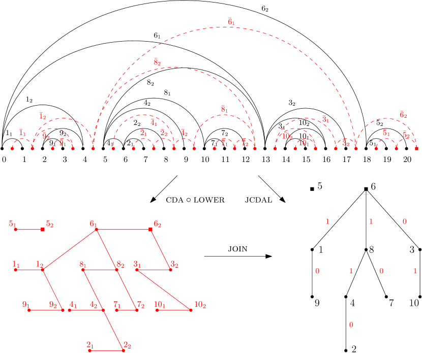
Figure 8. Let $f$ be the factorization given in Example 3.1. Displayed at the top in black is ${\textsc{arch}}\circ{\textsc{lower}}(f)$. At the top in red is ${\textsc{dual}}\circ{\textsc{arch}}\circ{\textsc{lower}}(f)$. At the bottom left is ${\textsc{cda}}\circ{\textsc{lower}}(f)$ and at the bottom right is ${\textsc{jcdal}}(f)\in\mathcal{R}_{10}^{2}$.

3.2. Proof of Theorem 1.2 (General Case)

We split the proof of Theorem 1.2 into two pieces. First we show that jcdal maps $(\mathrm{area}_{k},\mathrm{cosemiarea}_{k})$ to $k\cdot(\mathrm{maj}_{k},\mathrm{comaj})$, and later that it sends $(\mathrm{coarea}_{k},\mathrm{semiarea}_{k})\mapsto k\cdot(\mathrm{comaj}_{k},\mathrm{maj})$.

Proposition 3.3.

Let $f=(a_{1}^{0}\,\cdots\,a_{1}^{k})\cdots(a_{n}^{0}\,\cdots\,a_{n}^{k})\in\mathcal{F}_{n}^{k}$ and $F={\textsc{jcdal}}(f)\in\mathcal{R}_{n}^{k}$. Then $\mathrm{area}_{k}(f)=k\cdot\mathrm{maj}_{k}(F)$ and $\mathrm{cosemiarea}_{k}(f)=k\cdot\mathrm{comaj}(F)$. Moreover, $a_{j}^{k}-a_{j}^{0}=k\cdot h(j)$ for $j\in[1,n]$, where $h(j)$ is the hook length at $j$ in $F$.

Proof.

Let ${f^{*}}={\textsc{lower}}(f)$. Then by definition of area/coarea we have

$$\mathrm{area}({f^{*}})=\binom{kn}{2}-k\sum_{j=1}^{n}a^{0}_{j}, \mathrm{coarea}({f^{*}})=\sum_{i=1}^{k}\sum_{j=1}^{n}(a_{j}^{i}-1)-\binom{kn}{2},$$

and from the definition of $$\mathrm{area}_{k} \mathrm{coarea}_{k}$$ and , there follows

(11) $$\mathrm{area}_{k}(f)=\mathrm{area}({f^{*}})-n\binom{k}{2}, \mathrm{cosemiarea}_{k}(f)=\mathrm{coarea}({f^{*}}).$$

Now let $${F^{*}}={\textsc{cda}}({f^{*}}) F={\textsc{join}}({F^{*}})$$ and . Theorem 2.4 gives

(12) $$\mathrm{area}({f^{*}})=\mathrm{maj}({F^{*}}), \mathrm{coarea}({f^{*}})=\mathrm{comaj}({F^{*}}),$$

which together with (11) reduces the first claims of the proposition to the identities

(13) $$\mathrm{maj}({F^{*}})=n\binom{k}{2}+k\cdot\mathrm{maj}_{k}(F), \mathrm{comaj}({F^{*}})=k\cdot\mathrm{comaj}(F).$$

These will be verified below in Lemma 3.5, following an example. For the final claim of the proposition, observe that the factor $(a_{j}^{0}\,a_{j}^{k})$ of ${f^{*}}$ has label $j_{k}$, so Theorem 2.4 implies $a_{j}^{k}-a_{j}^{0}$ is the size of the hook at vertex $j_{k}$ in ${F^{*}}$. The definition of join makes clear that this is $k$ times the size of the hook at vertex $j$ of $F$. ∎

Example 3.4.

Continuing with Example 3.1, we have

$$\mathrm{area}_{k}(f) =\binom{kn}{2}-k\cdot\sum_{j}a^{0}_{j}-n\binom{k}{2}=190-2\cdot 73-10\cdot 1=34$$

$$\mathrm{cosemiarea}_{k}(f) =\sum_{i=1}^{k}\sum_{j=1}^{n}(a_{j}^{i}-1)-\binom{kn}{2}=202-190=12.$$

We also find that $\mathrm{area}({f^{*}})=44$ and $\mathrm{coarea}({f^{*}})=12$, and for ${F^{*}}$ in Figure 8 (bottom left) we have $\mathrm{maj}({F^{*}})=44$ and $\mathrm{comaj}({F^{*}})=12$, in agreement with (11) and (12).

The relevant statistics for $F={\textsc{jcdal}}(f)$ in Figure 8 (bottom right) are $\mathrm{maj}_{k}(F)=\mathrm{maj}(F)+\mathrm{chr}_{k}(F)=8+9=17$ and $\mathrm{comaj}(F)=6$. Comparing these with the values of $\mathrm{area}_{k}(f)$ and $\mathrm{cosemiarea}_{k}(f)$ above verifies the first claims Proposition 3.3. Note that $a_{8}^{k}-a_{0}^{k}=13-5=8$ while $h(8)=4$ in $F$, in accord with the second claim. ∎

To complete the proof of Proposition 3.3 we introduce the notion of a weighted $k$-forest. This is simply a $k$-forest $F$ together with a function $\mathrm{wt}:V(F)\rightarrow\{1,2,3,\ldots\}$ that assigns a positive integer weight to each vertex. We define the weighted hook length of a vertex $v$ in such a forest by $\bar{h}(v)=\sum_{u\in H(v)}\mathrm{wt}(u)$. This induces weighted versions of all statistics defined in terms of hook lengths, such as $\bar{h}_{L}(v)$, $\bar{h}_{R}(v)$, $\overline{\mathrm{maj}}(F)$, $\overline{\mathrm{maj}}_{k}(F)$, $\overline{\mathrm{chr}}_{k}(F)$ and so on.

Lemma 3.5.

Identities (13) are valid for any ${F^{*}}\in\mathcal{R}^{*}_{kn}$ and $F={\textsc{join}}({F^{*}})\in\mathcal{R}_{n}^{k}$.

Proof.

We begin with a general observation regarding weighted $k$-forests. Let $W$ be such a forest with edge colouring $\kappa:E(W)\rightarrow[k-1]$, and let edge $(x,y)\in E(W)$ be such that

• $x$ and $y$ have consecutive labels, with $x>y$, and

• $\kappa(x,y)=0$.

Let $W^{\prime}$ be the weighted $k$-forest obtained by collapsing edge $(x,y)$ as follows:

1. replace each edge $(y,v)$ with an edge $(x,v)$ coloured $\kappa(y,v)+1$,

2. increase $\mathrm{wt}(x)$ by $\mathrm{wt}(y)$, and

3. remove edge $(x,y)$ and vertex $y$.

This is illustrated in Figure 9. Our interest in this process arises from the fact that the join map can be viewed as iteratively collapsing edges of a weighted $k$-forest.

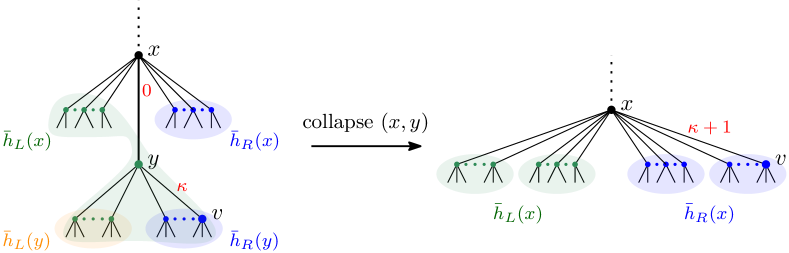
Figure 9. Collapsing edge $(x,y)$ of a weighted $k$-forest. Each edge $(y,v)$ with colour $\kappa$ is replaced by an edge $(x,v)$ with colour $\kappa+1$. The weight of vertex $x$ on the right is the sum of the weights of vertices $x$ and $y$ on the left.

Observe that collapsing $(x,y)$ leaves $\bar{h}_{L}(u)$ and $\bar{h}_{R}(u)$ unchanged for all vertices $u\neq x,y$, whereas $\bar{h}_{L}(x)$ and $\bar{h}_{R}(x)$ increase by $\bar{h}_{L}(y)-\bar{h}(y)$ and $\bar{h}_{R}(y)$, respectively, as a result of Condition (A). The net changes to major and comajor indices are therefore $(\bar{h}_{L}(y)-\bar{h}(y))-\bar{h}_{L}(y)=-\bar{h}(y)$ and $\bar{h}_{R}(y)-\bar{h}_{R}(y)=0$, respectively, where the terms $-\bar{h}_{L}(y)$ and $-\bar{h}_{R}(y)$ account for removal of $y$. That is,

(14) $$\overline{\mathrm{maj}}(W^{\prime})=\overline{\mathrm{maj}}(W)-\bar{h}(y)\qquad\text{and}\qquad\overline{\mathrm{comaj}}(W^{\prime})=\overline{\mathrm{comaj}}(W).$$

Using Condition (B) we also have

$$\overline{\mathrm{chr}}_{k}(W^{\prime}) =\overline{\mathrm{chr}}_{k}(W)-\underbrace{\kappa(x,y)}_{=0}\bar{h}(y)-\sum_{e=(y,v)}\kappa(e)\bar{h}(v)+\sum_{e=(y,v)}(\kappa(e)+1)\bar{h}(v)$$

(15) $$=\overline{\mathrm{chr}}_{k}(W)+\sum_{e=(y,v)}\bar{h}(v)$$

$$=\overline{\mathrm{chr}}_{k}(W)+\bar{h}(y)-\mathrm{wt}(y).$$

Together,  (14) and (3.2) give

(16) $$\overline{\mathrm{maj}}_{k}(W^{\prime})=\overline{\mathrm{maj}}_{k}(W)-\mathrm{wt}(y).$$

We are now prepared to prove the lemma. Let the vertices of ${F^{*}}$ be labelled by $S$ as defined in (8). Assign colour 0 to each edge of ${F^{*}}$ and weight 1 to each of its vertices to transform it into a weighted $k$-forest $W^{*}$. Clearly $\mathrm{maj}({F^{*}})=\overline{\mathrm{maj}}_{k}(W^{*})$ and $\mathrm{comaj}({F^{*}})=\overline{\mathrm{comaj}}(W^{*})$.

Transform $W^{*}$ by iteratively collapsing edges $(1_{2},1_{1}),(1_{3},1_{2}),\ldots,(1_{k},1_{k-1})$ in that order. This yields a sequence of forests $W^{*}=W_{1},W_{2},\ldots,W_{k}$ such that vertex $1_{i}$ has weight $i$ in $W_{i}$. Moreover, (14) and (16) give

$$\overline{\mathrm{comaj}}(W_{k})=\overline{\mathrm{comaj}}(W^{*})=\mathrm{comaj}(F^{*})$$

and

$$\overline{\mathrm{maj}}_{k}(W_{k})=\overline{\mathrm{maj}}_{k}(W^{*})-(1+2+\cdots+(k-1))=\mathrm{maj}({F^{*}})-\binom{k}{2}$$

Continue to iterate by collapsing edges $(j_{2},j_{1}),(j_{3},j_{2}),\ldots,(j_{k},j_{k-1})$, for each $j=2,\ldots,n$. When complete, this results in a weighted $k$-forest ${W}$ on vertices $\{1_{k},2_{k},\ldots,j_{k}\}$ such that

• every vertex has weight $k$,

• $\overline{\mathrm{maj}}_{k}(W)=\mathrm{maj}({F^{*}})-n\binom{k}{2}$, and

• $\overline{\mathrm{comaj}}(W)=\mathrm{comaj}({F^{*}})$.

Clearly ${W}$ is precisely the $k$-forest $F={\textsc{join}}({F^{*}})$ but with vertices weighted $k$, so we have $\overline{\mathrm{maj}}_{k}({W})=k\cdot\mathrm{maj}_{k}(F)$ and $\overline{\mathrm{comaj}}(W)=k\cdot\mathrm{comaj}(F)$. Therefore $\mathrm{maj}({F^{*}})=k\cdot\mathrm{maj}_{k}(F)+n\binom{k}{2}$ and $\mathrm{comaj}({F^{*}})=k\cdot\mathrm{comaj}(F)$, as desired. ∎

Finally, we prove the remainder of Theorem 1.2.

Proposition 3.6.

Let $f=(a_{1}^{0}\,\cdots\,a_{1}^{k})\cdots(a_{n}^{0}\,\cdots\,a_{n}^{k})\in\mathcal{F}_{n}^{k}$, and $F={\textsc{jcdal}}(f)$. Then $\mathrm{semiarea}_{k}(f)=k\cdot\mathrm{maj}(F)$ and $\mathrm{coarea}_{k}(f)=k\cdot\mathrm{comaj}_{k}(F)$.

Proof.

The proof is similar to that of Proposition 3.3, with one modification: we use a different though analogous intermediate function ${\textsc{upper}}:\mathcal{F}_{n}^{k}\rightarrow\mathcal{R}_{kn}$ defined by replacing each factor of a $k$-factorization with its upper decomposition; see (2). Thus if $f=(a_{1}^{0}\,\cdots\,a_{1}^{k})\cdots(a_{n}^{0}\,\cdots\,a_{n}^{k})\in\mathcal{F}_{n}^{k}$, then ${f^{\star}}:={\textsc{upper}}(f)$ is obtained by expanding the factor $(a_{j}^{0}\,\cdots a_{j}^{k})$ into $(a_{j}^{0}\,a_{j}^{k})(a_{j}^{1}\,a_{j}^{k})\cdots(a_{j}^{k-1}\,a_{j}^{k})$. We label the factors of ${f^{\star}}$ with the ordered set $S$ of (8), assigning factor $(a_{j}^{i}\;a_{j}^{k})$ the label $j_{i+1}$, and this labelling propagates to the resulting forests. We immediately obtain the relationship

(17) $$\mathrm{coarea}_{k}(f)=\mathrm{coarea}({f^{\star}})-n\cdot\binom{k}{2}\;\;\;\textnormal{ and }\;\;\;\mathrm{semiarea}_{k}(f)=\mathrm{area}({f^{\star}}),$$

which is analogous to (11). Clearly upper, like lower, is injective. Let ${\mathcal{R}}^{\star}_{kn}={\textsc{cda}}\circ{\textsc{upper}}({\mathcal{F}}^{\star}_{kn})$. Through the obvious analogue of Lemma 2.1, this subset of $\mathcal{R}_{kn}$ is seen to be characterized by

$${\mathcal{R}}^{\star}_{kn}=\{F\in\mathcal{R}_{n}^{k}\,:\,\text{vertex $j_{{i+1}}$ is a child of $j_{i}$ for all $j\in[1,n]$, $i\in[k-1]$}\}.$$

Setting ${F^{\star}}={\textsc{cda}}({f^{\star}})$, we know from Theorem 2.4 that

(18) $$\mathrm{coarea}({f^{\star}})=\mathrm{comaj}({F^{\star}})\qquad\textnormal{ and }\qquad\mathrm{area}({f^{\star}})=\mathrm{maj}({F^{\star}}).$$

We define ${\textsc{join}}:{\mathcal{R}}^{\star}_{kn}\rightarrow\mathcal{R}_{n}^{k}$ as before, and similar to Lemma 3.5 we find for $F={\textsc{join}}({F^{\star}})$ that

(19) $$\mathrm{comaj}({F^{\star}})=n\cdot\binom{k}{2}+k\cdot\mathrm{comaj}_{k}(F)\qquad\textnormal{ and }\qquad\mathrm{maj}({F^{\star}})=k\cdot\mathrm{maj}(F).$$

Finally, it is easy to see that the composition ${\textsc{join}}\circ{\textsc{cda}}\circ{\textsc{upper}}:\mathcal{F}_{n}^{k}\longrightarrow\mathcal{R}_{n}^{k}$ is precisely ${\textsc{jcdal}}:\mathcal{F}_{n}^{k}\longrightarrow\mathcal{R}_{n}^{k}$. Combining (17), (18) and (19) completes the proof. ∎

Example 3.7.

Let $f\in\mathcal{F}_{10}^{2}$ be as in Example 3.1. Then ${f^{\star}}={\textsc{upper}}(f)$ is

$${f^{\star}}=\underset{1_{1}}{(0\;4)}\underset{1_{2}}{(1\;4)}\underset{2_{1}}{(6\;8)}\underset{2_{2}}{(7\;8)}\underset{3_{1}}{(13\;17)}\underset{3_{2}}{(16\;17)}\underset{4_{1}}{(5\;9)} \underset{4_{2}}{(6\;9)}\underset{5_{1}}{(18\;20)}\underset{5_{2}}{(19\;20)}\underset{6_{1}}{(0\;18)}\underset{6_{2}}{(13\;18)}\underset{7_{1}}{(10\;12)}\underset{7_{2}}{(11\;12)}$$

$$\underset{8_{1}}{(5\;13)}\underset{8_{2}}{(10\;13)}\underset{9_{1}}{(2\;4)}\underset{9_{2}}{(3\;4)}\underset{10_{1}}{(14\;16)}\underset{10_{2}}{(15\;16)}.$$

The arch diagram of ${f^{\star}}$ and its dual are given in Figure 10. We see that

(20) $$\mathrm{coarea}_{k}(f) =k\sum_{j=1}^{n}(a_{j}^{k}-1)-\binom{kn}{2}-n\cdot\binom{k}{2}=222-190-10=22,$$

$$\mathrm{coarea}({f^{\star}}) =32,$$

confirming the first half of (17); also,

(21) $$\mathrm{semiarea}_{k}(f)=\binom{kn}{2}-\sum_{i=0}^{k-1}\sum_{j=1}^{n}a_{j}^{i}=190-174=16=\mathrm{area}({f^{\star}}),$$

confirming the second half. Figure 10 also shows ${F^{\star}}={\textsc{cda}}({f^{\star}})$ and $F={\textsc{jcdal}}(f)$. There we find $\mathrm{maj}({F^{\star}})=16$, $\mathrm{comaj}({F^{\star}})=32$, $\mathrm{maj}(F)=8$, and $\mathrm{comaj}_{k}(F)=\mathrm{comaj}(F)+{\mathrm{cochr}}_{k}(F)=6+5=11$. Comparison with (20) and (21) confirms (18) and (19). ∎

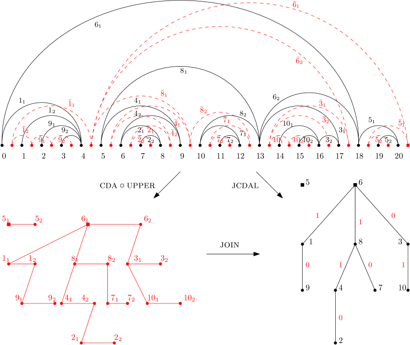
Figure 10. The arch diagram and dual of ${f^{\star}}={\textsc{upper}}(f)$, where $f$ is given in Example 3.1. Also shown are ${F^{\star}}={\textsc{cda}}({f^{\star}})$ (bottom left) and $F={\textsc{join}}({F^{\star}})={\textsc{jcdal}}(f)$ (bottom right).

References

- [Bia02] P. Biane, Parking functions of types A and B, Electron. J. Combin. 9 (2002).
- [BW89] A. Björner and M. L. Wachs, -Hook length formulas for forests, J. Combin. Theory Ser. A 52 (1989), 165–187.
- [Dé59] J. Dénes, The representation of a permutation as the product of a minimal number of transpositions and its connection with the theory of graphs, Publ. Math. Inst. Hungar. Acad. Sci. 4 (1959), 63–70.
- [GP16] A. Grady and S. Poznanović, Sorting index and Mahonian-Stirling pairs for labeled forests, Adv. in Appl. Math. 80 (2016), 93–113. MR 3537241
- [GS06] Ira M. Gessel and Seunghyun Seo, A refinement of Cayley’s formula for trees, Electron. J. Combin. 11 (2004/06), no. 2, Research Paper 27, 23. MR 2224940
- [GY02] I.P. Goulden and A. Yong, Tree-like properties of cycle factorizations, J. Combinat. Theory Ser. A. 98 (2002), 106–117.
- [Hag08] J. Haglund, The -catalan numbers and the space of diagonal harmonics: With an appendix on the combinatorics of macdonald polynomials, American Mathematical Society, 2008.
- [IR21] J. Irving and A. Rattan, Trees, parking functions and factorizations of the full cycle, European J. Combin. 93 (2021).
- [Irv09] J. Irving, Minimal transitive factorizations of permutations into cycles, Canad. J. Math. (2009), 1092–1117.
- [Kre80] G. Kreweras, Une famille de polynômes ayant plusiers propriétés énumeratives, Periodica Math. Hung. 11 (1980), 309–320.
- [LW92] K. Liang and M. L. Wachs, Mahonian statistics on labeled forests, Discrete Math. 99 (1992), 181–197.
- [MNW20] Henri Mühle, Philippe Nadeau, and Nathan Williams, -indivisible noncrossing partitions, Sém. Lothar. Combin. 81 (2020), Art. B81d, 23. MR 4097429
- [Mos89] P. Moszkowski, A solution to a problem of Dénes: a bijection between trees and factorizations of cyclic permutations, European J. Combinatorics 10 (1989), 13–16.
- [MR68] C. Mallows and J. Riordan, The inversion enumerator for labeled trees, Bull. Amer. Math. Soc. 74 (1968), 92–94.
- [Sta97] Richard P. Stanley, Parking functions and noncrossing partitions, Electron. J. Combin. 4 (1997), no. 2, Research Paper R20, 14 p., The Wilf Festschrift (Philadelphia, PA, 1996). MR 1444167
- [Yan97] C. H. Yan, Generalized tree inversions and -parking functions, J. Combin. Theory Ser. A 79 (1997), 268–280.
- [Yan15] by same author, Parking functions, The Handbook of Enumerative Combinatorics (M. Bóna, ed.), Discrete Math. Appl. (Boca Raton), CRC Press, 2015, p. 835–893. MR 3409354