Gradient Descent on Two-layer Nets:
Margin Maximization and Simplicity Bias

Abstract

The generalization mystery of overparametrized deep nets has motivated efforts to understand how gradient descent (GD) converges to low-loss solutions that generalize well. Real-life neural networks are initialized from small random values and trained with cross-entropy loss for classification (unlike the "lazy" or "NTK" regime of training where analysis was more successful), and a recent sequence of results [Lyu and Li, 2020, Chizat and Bach, 2020, Ji and Telgarsky, 2020a] provide theoretical evidence that GD may converge to the "max-margin" solution with zero loss, which presumably generalizes well. However, the global optimality of margin is proved only in some settings where neural nets are infinitely or exponentially wide. The current paper is able to establish this global optimality for two-layer Leaky ReLU nets trained with gradient flow on linearly separable and symmetric data, regardless of the width. The analysis also gives some theoretical justification for recent empirical findings [Kalimeris et al., 2019] on the so-called simplicity bias of GD towards linear or other "simple" classes of solutions, especially early in training. On the pessimistic side, the paper suggests that such results are fragile. A simple data manipulation can make gradient flow converge to a linear classifier with suboptimal margin.

1 Introduction

One major mystery in deep learning is why deep neural networks generalize despite overparameterization [Zhang et al., 2017]. To tackle this issue, many recent works turn to study the implicit bias of gradient descent (GD) — what kind of theoretical characterization can we give for the low-loss solution found by GD?

The seminal works by Soudry et al. [2018a, b] revealed an interesting connection between GD and margin maximization: for linear logistic regression on linearly separable data, there can be multiple linear classifiers that perfectly fit the data, but GD with any initialization always converges to the max-margin (hard-margin SVM) solution, even when there is no explicit regularization. Thus the solution found by GD has the same margin-based generalization bounds as hard-margin SVM. Subsequent works on linear models have extended this theoretical understanding of GD to SGD [Nacson et al., 2019b], other gradient-based methods [Gunasekar et al., 2018a], other loss functions with certain poly-exponential tails [Nacson et al., 2019a], linearly non-separable data [Ji and Telgarsky, 2018, 2019b], deep linear nets [Ji and Telgarsky, 2019a, Gunasekar et al., 2018b].

Given the above results, a natural question to ask is whether GD has the same implicit bias towards max-margin solutions for machine learning models in general. Lyu and Li [2020] studied the relationship between GD and margin maximization on deep homogeneous neural network, i.e., neural network whose output function is (positively) homogeneous with respect to its parameters. For homogeneous neural networks, only the direction of parameter matters for classification tasks. For logistic and exponential loss, Lyu and Li [2020] assumed that GD decreases the loss to a small value and achieves full training accuracy at some time point, and then provided an analysis for the training dynamics after this time point (Theorem 3.1), which we refer to as late phase analysis. It is shown that GD decreases the loss to $0$ in the end and converges to a direction satisfying the Karush-Kuhn-Tucker (KKT) conditions of a constrained optimization problem (P) on margin maximization.

However, given the non-convex nature of neural networks, KKT conditions do not imply global optimality for margins. Several attempts are made to prove the global optimality specifically for two-layer nets. Chizat and Bach [2020] provided a mean-field analysis for infinitely wide two-layer Squared ReLU nets showing that gradient flow converges to the solution with global max margin, which also corresponds to the max-margin classifier in some non-Hilbertian space of functions. Ji and Telgarsky [2020a] extended the proof to finite-width neural nets, but the width needs to be exponential in the input dimension (due to the use of a covering condition). Both works build upon late phase analyses. Under a restrictive assumption that the data is orthogonally separable, i.e., any data point ${\bm{x}}_{i}$ can serve as a perfect linear separator, Phuong and Lampert [2021] analyzed the full trajectory of gradient flow on two-layer ReLU nets with small initialization, and established the convergence to a piecewise linear classifier that maximizes the margin, irrespective of network width.

In this paper, we study the implicit bias of gradient flow on two-layer neural nets with Leaky ReLU activation [Maas et al., 2013] and logistic loss. To avoid the lazy or Neural Tangent Kernel (NTK) regime where the weights are initialized to large random values and do not change much during training [Jacot et al., 2018, Chizat et al., 2019, Du et al., 2019b, a, Allen-Zhu et al., 2018, 2019, Zou et al., 2018, Arora et al., 2019b], we use small initialization to encourage the model to learn features actively, which is closer to real-life neural network training.

When analyzing convergence behavior of training on neural networks, one can simplify the problem and gain insights by assuming that the data distribution has a simple structure. Many works particularly study the case where the labels are generated by an unknown teacher network that is much smaller/simpler than the (student) neural network to be trained. Following Brutzkus et al. [2018], Sarussi et al. [2021] and many other works, we consider the case where the dataset is linearly separable, namely the labels are generated by a linear teacher, and study the training dynamics of two-layer Leaky ReLU nets on such dataset.

1.1 Our Contribution

Among all the classifiers that can be represented by the two-layer Leaky ReLU nets, we show any global-max-margin classifier is exactly linear under one more data assumption: the dataset is symmetric, i.e., if ${\bm{x}}$ is in the training set, then so is $-{\bm{x}}$. Note that such symmetry can be ensured by simple data augmentation.

Still, little is known about what kind of classifiers neural network trained by GD learns. Though Lyu and Li [2020] showed that gradient flow converges to a classifier along KKT-margin direction, we note that this result is not sufficient to guarantee the global optimality since such classifier can have nonlinear decision boundaries. See Figure 1 (left) for an example.

In this paper, we provide a multi-phase analysis for the full trajectory of gradient flow, in contrast with previous late phase analyses which only analyzes the trajectory after achieving $100\%$ training accuracy. We show that gradient flow with small initialization converges to a global-max-margin linear classifier (Theorem 4.2). The proof leverages power iteration to show that neuron weights align in two directions in an early phase of training, inspired by Li et al. [2021]. We further show the alignment at any constant training time by associating the dynamics of wide neural net with that of two-neuron neural net, and finally, extend the alignment to the infinite time limit by applying Kurdyka-Łojasiewicz (KL) inquality in a similar way as Ji and Telgarsky [2020a]. The alignment at convergence implies that the convergent classifier is linear.

The above results also justify a recent line of works studying the so-called simplicity bias: GD first learns linear functions in the early phase of training, and the complexity of the solution increases as training goes on [Kalimeris et al., 2019, Hu et al., 2020, Shah et al., 2020]. Indeed, our result establishes a form of extreme simplicity bias of GD: if the dataset can be fitted by a linear classifier, then GD learns a linear classifier not only in the beginning but also at convergence.

On the pessimistic side, this paper suggests that such global margin maximization result could be fragile. Even for linearly separable data, global-max-margin classifiers may be nonlinear without the symmetry assumption. In particular, we show that for any linearly separable dataset, gradient flow can be led to converge to a linear classifier with suboptimal margin by adding only $3$ extra data points (Theorem 6.2). See Figure 1 (right) for an example.

2 Related Works

Generalization Aspect of Margin Maxmization.

Margin often appears in the generalization bounds for neural networks [Bartlett et al., 2017, Neyshabur et al., 2018], and larger margin leads to smaller bounds. Jiang et al. [2020] conducted an empirical study for the causal relationships between complexity measures and generalization errors, and showed positive results for normalized margin, which is defined by the output margin divided by the product (or powers of the sum) of Frobenius norms of weight matrices from each layer. On the pessimistic side, negative results are also shown if Frobenius norm is replaced by spectral norm. In this paper, we do use the normalized margin with Frobenius norm (see Section 3).

Learning on Linearly Separable Data.

Some works studied the training dynamics of (nonlinear) neural networks on linearly separable data (labels are generated by a linear teacher). Brutzkus et al. [2018] showed that SGD on two-layer Leaky ReLU nets with hinge loss fits the training set in finite steps and generalizes well. Frei et al. [2021] studied online SGD (taking a fresh sample from the population in each step) on the two-layer Leaky ReLU nets with logistic loss. For any data distribution, they proved that there exists a time step in the early phase such that the net has a test error competitive with that of the best linear classifier over the distribution, and hence generalizes well on linearly separable data. Both two papers reveal that the weight vectors in the first layer have positive correlations with the weight of the linear teacher, but their analyses do not imply that the learned classifier is linear. In the NTK regime, Ji and Telgarsky [2020b], Chen et al. [2021] showed that GD on shallow/deep neural nets learns a kernel predictor with good generalization on linearly separable data, and it suffices to have width polylogarithmic in the number of training samples. Still, they do not imply that the learned classifier is linear. Pellegrini and Biroli [2020] provided a mean-field analysis for two-layer ReLU net showing that training with hinge loss and infinite data leads to a linear classifier, but their analysis requires the data distribution to be spherically symmetric (i.e., the probability density only depends on the distance to origin), which is a more restrictive assumption than ours. Sarussi et al. [2021] provided a late phase analysis for gradient flow on two-layer Leaky ReLU nets with logistic loss, which establishes the convergence to linear classifier based on an assumption called Neural Agreement Regime (NAR): starting from some time point, for any training sample, the outputs of all the neurons have the same sign. However, it is unclear why this can happen a priori. Comparing with our work, we analyze the full trajectory of gradient flow and establish the convergence to linear classifier without assuming NAR. Phuong and Lampert [2021] analyzed the full trajectory for gradient flow on orthogonally separable data, but every KKT-margin direction attains the global max margin (see Appendix H) in their setting, which it is not necessarily true in general. In our setting, KKT-margin direction with suboptimal margin does exist.

Simplicity Bias.

Kalimeris et al. [2019] empirically observed that neural networks in the early phase of training are learning linear classifiers, and provided evidence that SGD learns functions of increasing complexity. Hu et al. [2020] justified this view by proving that the learning dynamics of two-layer neural nets and simple linear classifiers are close to each other in the early phase, for dataset drawn from a data distribution where input coordinates are independent after some linear transformation. The aforementioned work by Frei et al. [2021] can be seen as another theoretical justification for online SGD on aribitrary data distribution. Shah et al. [2020] pointed out that extreme simplicity bias can lead to suboptimal generalization and negative effects on adversarial robustness.

Small Initialization.

Several theoretical works studying neural network training with small initialization can be connected to simplicity bias. Maennel et al. [2018] uncovered a weight quantization effect in training two-layer nets with small initialization: gradient flow biases the weight vectors to a certain number of directions determined by the input data (independent of neural network width). It is hence argued that gradient flow has a bias towards “simple” functions, but their proof is not entirely rigorous and no clear definition of simplicity is given. This weight quantization effect has also been studied under the names of weight clustering [Brutzkus and Globerson, 2019], condensation [Luo et al., 2021, Xu et al., 2021]. Williams et al. [2019] studied univariate regression and showed that two-layer ReLU nets with small initialization tend to learn linear splines. For the matrix factorization problem, which can be related to training neural networks with linear or quadratic activations, we can measure the complexity of the learned solution by rank. A line of works showed that gradient descent learns solutions with gradually increasing rank [Li et al., 2018, Arora et al., 2019a, Gidel et al., 2019, Gissin et al., 2020, Li et al., 2021]. Such results have been generalized to tensor factorization where the complexity measure is replaced by tensor rank [Razin et al., 2021]. Beyond small initialization of our interest and large initialization in the lazy or NTK regime, Woodworth et al. [2020], Moroshko et al. [2020], Mehta et al. [2021] studied feature learning when the initialization scale transitions from small to large scale.

3 Preliminaries

We denote the set $\{1,\dots,n\}$ by $[n]$ and the unit sphere $\{{\bm{x}}\in\mathbb{R}^{d}:\|{\bm{x}}\|_{2}=1\}$ by $\mathbb{S}^{d-1}$. We call a function $h:\mathbb{R}^{D}\to\mathbb{R}$ $L$-homogeneous if $h(c{\bm{\theta}})=c^{L}h({\bm{\theta}})$ for all ${\bm{\theta}}\in\mathbb{R}^{D}$ and $c>0$. For $S\subseteq\mathbb{R}^{D}$, $\mathrm{conv}(S)$ denotes the convex hull of $S$. For locally Lipschitz function $f:\mathbb{R}^{D}\to\mathbb{R}$, we define Clarke’s subdifferential [Clarke, 1975, Clarke et al., 2008, Davis et al., 2020] to be $\partial^{\circ}f({\bm{\theta}}):=\mathrm{conv}\left\{\lim_{n\to\infty}\nabla f({\bm{\theta}}_{n}):f\text{ differentiable at }{\bm{\theta}}_{n},\lim_{n\to\infty}{\bm{\theta}}_{n}={\bm{\theta}}\right\}$ (see also Section B.1).

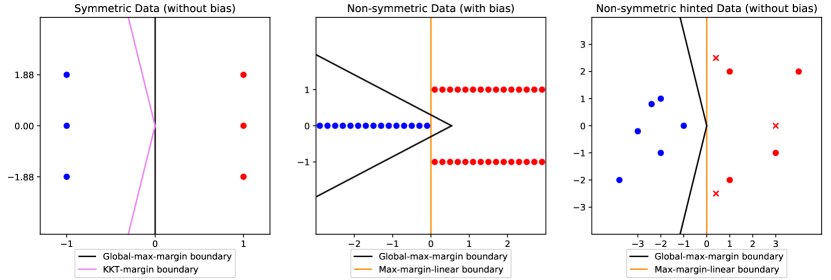
Figure 1: Two-layer Leaky ReLU nets ($\alpha_{\mathrm{leaky}}=1/2$) with KKT margin and global max margin on linearly separable data. See Section I.1 for detailed discussions. Left: Theorem 4.3 is not vacuous: a symmetric dataset can have KKT directions with suboptimal margin, but our theory shows that gradient flow from small initialization goes to global max margin. Middle: The linear classifier (orange) is along a KKT-margin direction with a much smaller margin comparing to the (nonlinear) global-max-margin classifier (black), but our theory suggests that gradient flow converges to the linear classifier. Right: Adding three extra data points (marked as “x”; see Definition 6.1) to a linearly separable dataset makes the linear classifier (orange) has suboptimal margin but causes the neural net to be biased to it.

3.1 Logistic Loss Minimization and Margin Maximization

For a neural net, we use $f_{{\bm{\theta}}}({\bm{x}})\in\mathbb{R}$ to denote the output logit on input ${\bm{x}}\in\mathbb{R}^{d}$ when the parameter is ${\bm{\theta}}\in\mathbb{R}^{D}$. We say that the neural net is $L$-homogeneous if $f_{{\bm{\theta}}}({\bm{x}})$ is $L$-homogeneous with respect to ${\bm{\theta}}$, i.e., $f_{c{\bm{\theta}}}({\bm{x}})=c^{L}f_{{\bm{\theta}}}({\bm{x}})$ for all ${\bm{\theta}}\in\mathbb{R}^{D}$ and $c>0$. VGG-like CNNs can be made homogeneous if we remove all the bias terms expect those in the first layer [Lyu and Li, 2020].

Throughout this paper, we restrict our attention to $L$-homogeneous neural nets with $f_{{\bm{\theta}}}({\bm{x}})$ definable with respect to ${\bm{\theta}}$ in an o-minimal structure for all ${\bm{x}}$. (See Coste 2000 for reference for o-minimal structures.) This is a technical condition needed by Theorem 3.1, and it is a mild regularity condition as almost all modern neural networks satisfy this condition, including the two-layer Leaky ReLU networks studied in this paper.

For a dataset $\mathcal{S}=\{({\bm{x}}_{1},y_{1}),\dots,({\bm{x}}_{n},y_{n})\}$, we define $q_{i}({\bm{\theta}}):=y_{i}f_{{\bm{\theta}}}({\bm{x}}_{i})$ to be the output margin on the data point $({\bm{x}}_{i},y_{i})$, and $q_{\min}({\bm{\theta}}):=\min_{i\in[n]}q_{i}({\bm{\theta}})$ to be the output margin on the dataset $\mathcal{S}$ (or margin for short). It is easy to see that $q_{1}({\bm{\theta}}),\dots,q_{n}({\bm{\theta}})$ are $L$-homogeneous functions, and so is $q_{\min}({\bm{\theta}})$. We define the normalized margin $\gamma({\bm{\theta}}):=q_{\min}\left(\frac{{\bm{\theta}}}{\|{\bm{\theta}}\|_{2}}\right)=\frac{q_{\min}({\bm{\theta}})}{\|{\bm{\theta}}\|_{2}^{L}}$ to be the output margin (on the dataset) for the normalized parameter $\frac{{\bm{\theta}}}{\|{\bm{\theta}}\|_{2}}$.

We refer the problem of finding ${\bm{\theta}}$ that maximizes $\gamma({\bm{\theta}})$ as margin maximization. Note that once we have found an optimal solution ${\bm{\theta}}^{*}\in\mathbb{R}^{D}$, $c{\bm{\theta}}^{*}$ is also optimal for all $c>0$. We can put the norm constraint on ${\bm{\theta}}$ to eliminate this freedom on rescaling:

$$\max_{{\bm{\theta}}\in\mathbb{S}^{D-1}}~{}~{}\gamma({\bm{\theta}}).$$ (M)

Alternatively, we can also constrain the margin to have $q_{\min}\geq 1$ and minimize the norm:

$$\min~{}~{}\frac{1}{2}\|{\bm{\theta}}\|_{2}^{2}\quad\text{s.t.}\quad q_{i}({\bm{\theta}})\geq 1,\quad\forall i\in[n].$$ (P)

One can easily show that ${\bm{\theta}}^{*}$ is a global maximizer of (M) if and only if $\frac{{\bm{\theta}}^{*}}{(q_{\min}({\bm{\theta}}^{*}))^{1/L}}$ is a global minimizer of (P). For convenience, we make the following convention: if $\frac{{\bm{\theta}}}{\|{\bm{\theta}}\|_{2}}$ is a local/global maximizer of (M), then we say ${\bm{\theta}}$ is along a local-max-margin direction/global-max-margin direction; if $\frac{{\bm{\theta}}}{(q_{\min}({\bm{\theta}}))^{1/L}}$ satisfies the KKT conditions of (P), then we say ${\bm{\theta}}$ is along a KKT-margin direction.

Gradient flow with logistic loss is defined by the following differential inclusion,

$$\frac{\textup{{d}}{\bm{\theta}}}{\textup{{d}}t}\in-\partial^{\circ}\mathcal{L}({\bm{\theta}}),\quad\textrm{with }\mathcal{L}({\bm{\theta}}):=\frac{1}{n}\sum_{i=1}^{n}\ell(q_{i}({\bm{\theta}})),$$ (1)

where $\ell(q):=\ln(1+e^{-q})$ is the logistic loss. Lyu and Li [2020], Ji and Telgarsky [2020a] showed that ${\bm{\theta}}(t)/\|{\bm{\theta}}(t)\|_{2}$ always converges to a KKT-margin direction. We restate the results below.

Theorem 3.1 (Lyu and Li 2020, Ji and Telgarsky 2020a).

For homogeneous neural networks, if $\mathcal{L}({\bm{\theta}}(0))<\frac{\ln 2}{n}$, then $\mathcal{L}({\bm{\theta}}(t))\to 0$, $\|{\bm{\theta}}(t)\|_{2}\to+\infty$, and $\frac{{\bm{\theta}}(t)}{\|{\bm{\theta}}(t)\|_{2}}$ converges to a KKT-margin direction as $t\to+\infty$.

3.2 Two-Layer Leaky ReLU Networks on Linearly Separable Data

Let $\phi(x)=\max\{x,\alpha_{\mathrm{leaky}}x\}$ be Leaky ReLU, where $\alpha_{\mathrm{leaky}}\in(0,1)$. Throughout the following sections, we consider a two-layer neural net defined as below,

$$f_{{\bm{\theta}}}({\bm{x}})=\sum_{k=1}^{m}a_{k}\phi({\bm{w}}_{k}^{\top}{\bm{x}}).$$

where ${\bm{w}}_{1},\dots,{\bm{w}}_{m}\in\mathbb{R}^{d}$ are the weights in the first layer, $a_{1},\dots,a_{m}\in\mathbb{R}$ are the weights in the second layer, and ${\bm{\theta}}=({\bm{w}}_{1},\dots,{\bm{w}}_{m},a_{1},\dots,a_{m})\in\mathbb{R}^{D}$ is the concatenation of all trainable parameters, where $D=md+m$. We can verify that $f_{{\bm{\theta}}}({\bm{x}})$ is $2$-homogeneous with respect to ${\bm{\theta}}$.

Let $\mathcal{S}:=\{({\bm{x}}_{1},y_{1}),\dots,({\bm{x}}_{n},y_{n})\}$ be the training set. For simplicity, we assume that $\|{\bm{x}}_{i}\|_{2}\leq 1$. We focus on linearly separable data, thus we assume that $\mathcal{S}$ is linearly separable throughout the paper.

Assumption 3.2 (Linear Separable).

There exists a ${\bm{w}}\in\mathbb{R}^{d}$ such that $y_{i}\left<{\bm{w}},{\bm{x}}_{i}\right>\geq 1$ for all $i\in[n]$.

Definition 3.3 (Max-margin Linear Separator).

For the linearly separable dataset $\mathcal{S}$, we say that ${\bm{w}}^{*}\in\mathbb{S}^{d-1}$ is the max-margin linear separator if ${\bm{w}}^{*}$ maximizes $\min_{i\in[n]}y_{i}\left<{\bm{w}},{\bm{x}}_{i}\right>$ over ${\bm{w}}\in\mathbb{S}^{d-1}$.

4 Training on Linearly Separable and Symmetric Data

In this section, we study the implicit bias of gradient flow assuming the training data is linearly separable and symmetric. We say a dataset is symmetric if whenever ${\bm{x}}$ is present in the training set, the input $-{\bm{x}}$ is also present. By linear separability, ${\bm{x}}$ and $-{\bm{x}}$ must have different labels because $\left<{\bm{w}}^{*},{\bm{x}}\right>=-\left<{\bm{w}}^{*},-{\bm{x}}\right>$, where ${\bm{w}}^{*}$ is the max-margin linear separator. The formal statement for this assumption is given below.

Assumption 4.1 (Symmetric).

$n$ is even and ${\bm{x}}_{i}=-{\bm{x}}_{i+n/2},y_{i}=1,y_{i+n/2}=-1$ for $1\leq i\leq n/2$.

This symmetry can be ensured via data augmentation. Given a dataset, if it is known that the ground-truth labels are produced by an unknown linear classifier, then one can augment each data point $({\bm{x}},y)$ by flipping the sign, i.e., replace it with two data points $({\bm{x}},y)$, $(-{\bm{x}},-y)$ (and thus the dataset size is doubled).

Our results show that gradient flow directionally converges to a global-max-margin direction for two-layer Leaky ReLU networks, when the dataset is linearly separable and symmetric. To achieve such result, the key insight is that any global-max-margin direction represents a linear classifier, which we will see in Section 4.1. Then we will present our main convergence results in Section 4.2.

4.1 Global-Max-Margin Classifiers are Linear

Theorem 4.2 below characterizes the global-max-margin direction in our case by showing that margin maximization and simplicity bias coincide with each other: a network that representing the max-margin linear classifier (i.e., $f_{{\bm{\theta}}}({\bm{x}})=c\left<{\bm{w}}^{*},{\bm{x}}\right>$ for some $c>0$) can simultaneously achieve the goals of being simple and maximizing the margin.

Theorem 4.2.

Under Assumptions 3.2 and 4.1, for the two-layer Leaky ReLU network with width $m\geq 2$, any global-max-margin direction ${\bm{\theta}}^{*}\in\mathbb{S}^{D-1}$, $f_{{\bm{\theta}}^{*}}$ represents a linear classifier. Moreover, we have $f_{{\bm{\theta}}^{*}}({\bm{x}})=\frac{1+\alpha_{\mathrm{leaky}}}{4}\left<{\bm{w}}^{*},{\bm{x}}\right>$ for all ${\bm{x}}\in\mathbb{R}^{d}$, where ${\bm{w}}^{*}$ is the max-margin linear separator.

The result of Theorem 4.2 is based on the observation that replacing each neuron $(a_{k},{\bm{w}}_{k})$ in a network with two neurons of oppositing parameters $(a_{k},{\bm{w}}_{k})$ and $(-a_{k},-{\bm{w}}_{k})$ does not decrease the normalized margin on the symmetric dataset, while making the classifier linear in function space. Thus if any direction attains the global max margin, we can construct a new global-max-margin direction which corresponds to a linear classifier. We can show that every weight vector ${\bm{w}}_{k}$ of this linear classifier must be in the direction of ${\bm{w}}^{*}$ or $-{\bm{w}}^{*}$. Then the original classifier must also be linear in the same direction.

4.2 Convergence to Global-Max-Margin Directions

Though Theorem 3.1 guarantees that gradient flow directionally converges to a KKT-margin direction if the loss is optimized successfully, we note that KKT-margin directions can be non-linear and have complicated decision boundaries. See Figure 1 (left) for an example. Therefore, to establish the convergence to linear classifiers, Theorem 3.1 is not enough and we need a new analysis for the trajectory of gradient flow.

We use initialization ${\bm{w}}_{k}\overset{\text{i.i.d.}}{\sim}\mathcal{N}({\bm{0}},\sigma_{\mathrm{init}}^{2}{\bm{I}})$, $a_{k}\overset{\text{i.i.d.}}{\sim}\mathcal{N}(0,c_{\mathrm{ainit}}^{2}\sigma_{\mathrm{init}}^{2})$, where $c_{\mathrm{ainit}}$ is a fixed constant throughout this paper and $\sigma_{\mathrm{init}}$ controls the initialization scale. We call this distribution as ${\bm{\theta}}_{0}\sim\mathcal{D}_{\mathrm{init}}(\sigma_{\mathrm{init}})$. An alternative way to generate this distribution is to first draw $\bar{{\bm{\theta}}}_{0}\sim\mathcal{D}_{\mathrm{init}}(1)$, and then set ${\bm{\theta}}_{0}=\sigma_{\mathrm{init}}\bar{{\bm{\theta}}}_{0}$. With small initialization, we can establish the following convergence result.

Theorem 4.3.

Under Assumptions 3.2 and 4.1 and certain regularity conditions (see Assumptions 4.5 and 4.6 below), consider gradient flow on a Leaky ReLU network with width $m\geq 2$ and initialization ${\bm{\theta}}_{0}=\sigma_{\mathrm{init}}\bar{{\bm{\theta}}}_{0}$ where $\bar{{\bm{\theta}}}_{0}\sim\mathcal{D}_{\mathrm{init}}(1)$. With probability $1-2^{-(m-1)}$ over the random draw of $\bar{{\bm{\theta}}}_{0}$, if the initialization scale is sufficiently small, then gradient flow directionally converges and $f^{\infty}({\bm{x}}):=\lim_{t\to+\infty}f_{{\bm{\theta}}(t)/\|{\bm{\theta}}(t)\|_{2}}({\bm{x}})$ represents the max-margin linear classifier. That is,

$$\Pr_{\bar{{\bm{\theta}}}_{0}\sim\mathcal{D}_{\mathrm{init}}(1)}\left[\exists\sigma_{\mathrm{init}}^{\max}>0\text{ s.t. }\forall\sigma_{\mathrm{init}}<\sigma_{\mathrm{init}}^{\max},\forall{\bm{x}}\in\mathbb{R}^{d},f^{\infty}({\bm{x}})=C\left<{\bm{w}}^{*},{\bm{x}}\right>\right]\geq 1-2^{-(m-1)},$$

where $C:=\frac{1+\alpha_{\mathrm{leaky}}}{4}$ is a scaling factor.

Combining Theorem 4.2 and Theorem 4.3, we can conclude that gradient flow achieves the global max margin in our case.

Corollary 4.4.

In the settings of Theorem 4.3, gradient flow on linearly separable and symmetric data directionally converges to the global-max-margin direction with probability $1-2^{-(m-1)}$.

4.3 Additional Notations and Assumptions

Let ${\bm{\mu}}:=\frac{1}{n}\sum_{i=1}^{n}y_{i}{\bm{x}}_{i}$, which is non-zero since $\left<{\bm{\mu}},{\bm{w}}_{*}\right>=\frac{1}{n}\sum_{i\in[n]}y_{i}{\bm{w}}_{*}^{\top}{\bm{x}}_{i}\geq 1$. Let $\bar{{\bm{\mu}}}:=\frac{{\bm{\mu}}}{\|{\bm{\mu}}\|_{2}}$. We use $\varphi({\bm{\theta}}_{0},t)\in\mathbb{R}^{d}$ to the value of ${\bm{\theta}}$ at time $t$ for ${\bm{\theta}}(0)={\bm{\theta}}_{0}$.

We make the following technical assumption, which holds if we are allowed to add a slight perturbation to the training set.

Assumption 4.5.

For all $i\in[n]$, $\left<{\bm{\mu}},{\bm{x}}_{i}\right>\neq 0$.

Another technical issue we face is that the gradient flow may not be unique due to non-smoothness. It is possible that $\varphi({\bm{\theta}}_{0},t)$ is not well-defined as the solution of (1) may not be unique. See Section I.2 for more discussions. In this case, we assign $\varphi({\bm{\theta}}_{0},\,\cdot\,)$ to be an arbitrary gradient flow trajectory starting from ${\bm{\theta}}_{0}$. In the case where $\varphi({\bm{\theta}}_{0},t)$ has only one possible value for all $t\geq 0$, we say that ${\bm{\theta}}_{0}$ is a non-branching starting point. We assume the following technical assumption.

Assumption 4.6.

For any $m\geq 2$, there exist $r,\epsilon>0$ such that ${\bm{\theta}}$ is a non-branching starting point if its neurons can be partitioned into two groups: in the first group, $a_{k}=\|{\bm{w}}_{k}\|_{2}\in(0,r)$ and all ${\bm{w}}_{k}$ point to the same direction ${\bm{w}}^{+}\in\mathbb{S}^{d-1}$ with $\|{\bm{w}}^{+}-\bar{{\bm{\mu}}}\|_{2}\leq\epsilon$; in the second group, $-a_{k}=\|{\bm{w}}_{k}\|_{2}\in(0,r)$ and all ${\bm{w}}_{k}$ point to the same direction ${\bm{w}}^{-}\in\mathbb{S}^{d-1}$ with $\|{\bm{w}}^{-}+\bar{{\bm{\mu}}}\|_{2}\leq\epsilon$.

5 Proof Sketch for the Symmetric Case

In this section, we provide a proof sketch for Theorem 4.3. Our proof uses a multi-phase analysis, which divides the training process into $3$ phases, from small initialization to the final convergence. We will now elaborate the analyses for them one by one.

5.1 Phase I: Dynamics Near Zero

Gradient flow starts with small initialization. In Phase I, we analyze the dynamics when gradient flow does not go far away from zero. Inspired by Li et al. [2021], we relate such dynamics to power iterations and show that every weight vector ${\bm{w}}_{k}$ in the first layer moves towards the directions of either $\bar{{\bm{\mu}}}$ or $-\bar{{\bm{\mu}}}$. To see this, the first step is to note that $f_{{\bm{\theta}}}({\bm{x}}_{i})\approx 0$ when ${\bm{\theta}}$ is close to ${\bm{0}}$. Applying Taylor expansion on $\ell(y_{i}f_{{\bm{\theta}}}({\bm{x}}_{i}))$,

$$\mathcal{L}({\bm{\theta}})=\frac{1}{n}\sum_{i\in[n]}\ell(y_{i}f_{{\bm{\theta}}}({\bm{x}}_{i}))\approx\frac{1}{n}\sum_{i\in[n]}\left(\ell(0)+\ell^{\prime}(0)y_{i}f_{{\bm{\theta}}}({\bm{x}}_{i})\right).$$ (2)

Expanding $f_{{\bm{\theta}}}({\bm{x}}_{i})$ and reorganizing the terms, we have

$$\mathcal{L}({\bm{\theta}})\approx\frac{1}{n}\sum_{i\in[n]}\ell(0)+\frac{1}{n}\sum_{i\in[n]}\ell^{\prime}(0)\sum_{k\in[m]}y_{i}a_{k}\phi({\bm{w}}_{k}^{\top}{\bm{x}}_{i}) =\ell(0)+\frac{\ell^{\prime}(0)}{n}\sum_{k\in[m]}\sum_{i\in[n]}y_{i}a_{k}\phi({\bm{w}}_{k}^{\top}{\bm{x}}_{i})$$

$$=\ell(0)-\sum_{k\in[m]}a_{k}G({\bm{w}}_{k}),$$

where $G$-function [Maennel et al., 2018] is defined below:

$$G({\bm{w}}):=\frac{-\ell^{\prime}(0)}{n}\sum_{i\in[n]}y_{i}\phi({\bm{w}}^{\top}{\bm{x}}_{i})=\frac{1}{2n}\sum_{i\in[n]}y_{i}\phi({\bm{w}}^{\top}{\bm{x}}_{i}).$$

This means gradient flow optimizes each $-a_{k}G({\bm{w}}_{k})$ separately near origin.

$$\frac{\textup{{d}}{\bm{w}}_{k}}{\textup{{d}}t}\approx a_{k}\partial^{\circ}G({\bm{w}}_{k}),\qquad\frac{\textup{{d}}a_{k}}{\textup{{d}}t}\approx G({\bm{w}}_{k}).$$ (3)

In the case where Assumption 4.1 holds, we can pair each ${\bm{x}}_{i}$ with $-{\bm{x}}_{i}$ and use the identity $\phi(z)-\phi(-z)=\max\{z,\alpha_{\mathrm{leaky}}z\}-\max\{-z,-\alpha_{\mathrm{leaky}}z\}=(1+\alpha_{\mathrm{leaky}})z$ to show that $G({\bm{w}})$ is linear:

$$G({\bm{w}})=\frac{1}{2n}\sum_{i\in[n/2]}\left(\phi({\bm{w}}^{\top}{\bm{x}}_{i})-\phi(-{\bm{w}}^{\top}{\bm{x}}_{i})\right) =\frac{1}{2n}\sum_{i\in[n/2]}(1+\alpha_{\mathrm{leaky}}){\bm{w}}^{\top}{\bm{x}}_{i}=\left<{\bm{w}},\tilde{{\bm{\mu}}}\right>,$$

where $\tilde{{\bm{\mu}}}:=\frac{1+\alpha_{\mathrm{leaky}}}{2}{\bm{\mu}}=\frac{1+\alpha_{\mathrm{leaky}}}{2n}\sum_{i\in[n]}y_{i}{\bm{x}}_{i}$. Substituting this formula for $G$ into (3) reveals that the dynamics of two-layer neural nets near zero has a close relationship to power iteration (or matrix exponentiation) of a matrix ${\bm{M}}_{\tilde{{\bm{\mu}}}}\in\mathbb{R}^{(d+1)\times(d+1)}$ that only depends on data.

$$\frac{\textup{{d}}}{\textup{{d}}t}\begin{bmatrix}{\bm{w}}_{k}\\ a_{k}\end{bmatrix}\approx{\bm{M}}_{\tilde{{\bm{\mu}}}}\begin{bmatrix}{\bm{w}}_{k}\\ a_{k}\end{bmatrix},\qquad\text{where}\qquad{\bm{M}}_{\tilde{{\bm{\mu}}}}:=\begin{bmatrix}{\bm{0}}&\tilde{{\bm{\mu}}}\\ \tilde{{\bm{\mu}}}^{\top}&0\end{bmatrix}.$$

Simple linear algebra shows that $\lambda_{0}:=\|\tilde{{\bm{\mu}}}\|_{2}$, $\frac{1}{\sqrt{2}}(\bar{{\bm{\mu}}},1)\in\mathbb{R}^{d+1}$ are the unique top eigenvalue and eigenvector of ${\bm{M}}_{\tilde{{\bm{\mu}}}}$, which suggests that $({\bm{w}}_{k}(t),a_{k}(t))\in\mathbb{R}^{d+1}$ aligns to this top eigenvector direction if the approximation (3) holds for a sufficiently long time. With small initialization, this can indeed be true and we obtain the following lemma.

Definition 5.1 (M-norm).

For parameter vector ${\bm{\theta}}=({\bm{w}}_{1},\dots,{\bm{w}}_{m},a_{1},\dots,a_{m})$, we define the M-norm to be $\|{\bm{\theta}}\|_{\mathrm{M}}=\max_{k\in[m]}\left\{\max\{\|{\bm{w}}_{k}\|_{2},\lvert a_{k}\rvert\}\right\}$.

Lemma 5.2.

Let $r>0$ be a small value. With probability $1$ over the random draw of $\bar{{\bm{\theta}}}_{0}=(\bar{\bm{w}}_{1},\dots,\bar{{\bm{w}}}_{m},\bar{a}_{1},\dots,\bar{a}_{m})\sim\mathcal{D}_{\mathrm{init}}(1)$, if we take $\sigma_{\mathrm{init}}\leq\frac{r^{3}}{\sqrt{m}\left\|\bar{{\bm{\theta}}}_{0}\right\|_{\mathrm{M}}}$, then any neuron $({\bm{w}}_{k},a_{k})$ at time $T_{1}(r):=\frac{1}{\lambda_{0}}\ln\frac{r}{\sqrt{m}\sigma_{\mathrm{init}}\left\|\bar{{\bm{\theta}}}_{0}\right\|_{\mathrm{M}}}$ can be decomposed into

$${\bm{w}}_{k}(T_{1}(r))=r\bar{b}_{k}\bar{{\bm{\mu}}}+\Delta{\bm{w}}_{k},\qquad a_{k}(T_{1}(r))=r\bar{b}_{k}+\Delta a_{k},$$

where $\bar{b}_{k}:=\frac{\langle\bar{{\bm{w}}}_{k},\bar{{\bm{\mu}}}\rangle+\bar{a}_{k}}{2\sqrt{m}\left\|\bar{{\bm{\theta}}}_{0}\right\|_{\mathrm{M}}}$ and the error term $\Delta{\bm{\theta}}:=(\Delta{\bm{w}}_{1},\dots,\Delta{\bm{w}}_{m},\Delta a_{1},\dots,\Delta a_{m})$ is bounded by $\|\Delta{\bm{\theta}}\|_{\mathrm{M}}\leq\frac{Cr^{3}}{\sqrt{m}}$ for some universal constant $C$.

5.2 Phase II: Near-Two-Neuron Dynamics

By Lemma 5.2, we know that at time $T_{1}(r)$ we have ${\bm{w}}_{k}(T_{1}(r))\approx r\bar{b}_{k}\bar{{\bm{\mu}}}$ and $a_{k}(T_{1}(r))\approx r\bar{b}_{k}$, where $\bar{{\bm{b}}}\in\mathbb{R}^{d}$ is some fixed vector. This motivates us to couple the training dynamics of ${\bm{\theta}}(t)=({\bm{w}}_{1}(t),\dots,{\bm{w}}_{m}(t),a_{1}(t),\dots,a_{m}(t))$ after the time $T_{1}(r)$ with another gradient flow starting from the point $(r\bar{b}_{1}\bar{{\bm{\mu}}},\dots,r\bar{b}_{m}\bar{{\bm{\mu}}},r\bar{b}_{1},\dots,r\bar{b}_{m})$. Interestingly, the latter dynamic can be seen as a dynamic of two neurons “embedded” into the $m$-neuron neural net, and we will show that ${\bm{\theta}}(t)$ is close to this “embedded” two-neuron dynamic for a long time. Now we first introduce our idea of embedding a two-neuron network into an $m$-neuron network.

Embedding.

For any ${\bm{b}}\in\mathbb{R}^{m}$, we say that ${\bm{b}}$ is a good embedding vector if it has at least one positive entry and one negative entry, and all the entries are non-zero. For a good embedding vector ${\bm{b}}$, we use $b_{+}:=\sqrt{\sum_{j\in[m]}\mathbbm{1}_{[b_{j}>0]}b_{j}^{2}}$ and $b_{-}:=-\sqrt{\sum_{j\in[m]}\mathbbm{1}_{[b_{j}<0]}b_{j}^{2}}$ to denote the root-sum-squared of the positive entries and the negative root-sum-squared of the negative entries. For parameter $\hat{{\bm{\theta}}}:=(\hat{{\bm{w}}}_{1},\hat{{\bm{w}}}_{2},\hat{a}_{1},\hat{a}_{2})$ of a two-neuron neural net with $\hat{a}_{1}>0$ and $\hat{a}_{2}<0$, we define the embedding from two-neuron into $m$-neuron neural nets as $\pi_{{\bm{b}}}(\hat{{\bm{w}}}_{1},\hat{{\bm{w}}}_{2},\hat{a}_{1},\hat{a}_{2})=({\bm{w}}_{1},\dots,{\bm{w}}_{m},a_{1},\dots,a_{m})$, where

$$a_{k}=\begin{cases}\frac{b_{k}}{b_{+}}\hat{a}_{1},&\textrm{if }b_{k}>0\\ \frac{b_{k}}{b_{-}}\hat{a}_{2},&\textrm{if }b_{k}<0\\ \end{cases},\qquad{\bm{w}}_{k}=\begin{cases}\frac{b_{k}}{b_{+}}\hat{{\bm{w}}}_{1},&\textrm{if }b_{k}>0\\ \frac{b_{k}}{b_{-}}\hat{{\bm{w}}}_{2},&\textrm{if }b_{k}<0\\ \end{cases}.$$

It is easy to check that $f_{\hat{{\bm{\theta}}}}({\bm{x}})=f_{\pi_{{\bm{b}}}(\hat{{\bm{\theta}}})}({\bm{x}})$ by the homogeneity of the activation ($\phi(cz)=c\phi(z)$ for $c>0$):

$$f_{\pi_{{\bm{b}}}(\hat{{\bm{\theta}}})}({\bm{x}}) =\sum_{b_{k}>0}a_{k}\phi({\bm{w}}_{k}^{\top}{\bm{x}})+\sum_{b_{k}<0}a_{k}\phi({\bm{w}}_{k}^{\top}{\bm{x}})$$

$$=\sum_{b_{k}>0}\frac{b_{k}^{2}}{b_{+}^{2}}\hat{a}_{1}\phi(\hat{{\bm{w}}}_{1}^{\top}{\bm{x}})+\sum_{b_{k}<0}\frac{b_{k}^{2}}{b_{-}^{2}}\hat{a}_{2}\phi(\hat{{\bm{w}}}_{2}^{\top}{\bm{x}})=\hat{a}_{1}\phi(\hat{{\bm{w}}}_{1}^{\top}{\bm{x}})+\hat{a}_{2}\phi(\hat{{\bm{w}}}_{2}^{\top}{\bm{x}})=f_{\hat{{\bm{\theta}}}}({\bm{x}}).$$

Moreover, by taking the chain rule, we can obtain the following lemma showing that the trajectories starting from $\hat{{\bm{\theta}}}$ and $\pi_{{\bm{b}}}(\hat{{\bm{\theta}}})$ are essentially the same.

Lemma 5.3.

Given $\hat{{\bm{\theta}}}:=(\hat{{\bm{w}}}_{1},\hat{{\bm{w}}}_{2},\hat{a}_{1},\hat{a}_{2})$ with $\hat{a}_{1}>0$ and $\hat{a}_{2}<0$, if both $\hat{{\bm{\theta}}}$ and $\pi_{{\bm{b}}}(\hat{{\bm{\theta}}})$ are non-branching starting points, then $\varphi(\pi_{{\bm{b}}}(\hat{{\bm{\theta}}}),t)=\pi_{{\bm{b}}}(\varphi(\hat{{\bm{\theta}}},t))$ for all $t\geq 0$.

Approximate Embedding.

Back to our analysis for Phase II, $\bar{{\bm{b}}}$ is a good embedding vector with high probability (see lemma below). Let $\hat{{\bm{\theta}}}:=(\bar{b}_{+},\bar{b}_{+}\bar{{\bm{\mu}}},\bar{b}_{-},\bar{b}_{-}\bar{{\bm{\mu}}})$. By Lemma 5.2, $\pi_{\bar{{\bm{b}}}}(r\hat{{\bm{\theta}}})=(r\bar{b}_{1}\bar{{\bm{\mu}}},\dots,r\bar{b}_{m}\bar{{\bm{\mu}}},r\bar{b}_{1},\dots,r\bar{b}_{m})\approx{\bm{\theta}}(T_{1}(r))$, which means $r\hat{{\bm{\theta}}}\to{\bm{\theta}}(T_{1}(r))$ is approximately an embedding. Suppose that the approximation happens to be exact, namely $\pi_{\bar{{\bm{b}}}}(r\hat{{\bm{\theta}}})={\bm{\theta}}(T_{1}(r))$, then ${\bm{\theta}}(T_{1}(r)+t)=\pi_{\bar{{\bm{b}}}}(\varphi(r\hat{{\bm{\theta}}},t))$ by Lemma 5.3. Inspired by this, we consider the case where $\sigma_{\mathrm{init}}\to 0,r\to 0$ so that the approximate embedding is infinitely close to the exact one, and prove the following lemma. We shift the training time by $T_{2}(r)$ to avoid trivial limits (such as ${\bm{0}}$).

Lemma 5.4.

Follow the notations in Lemma 5.2 and take $\sigma_{\mathrm{init}}\leq\frac{r^{3}}{\sqrt{m}\left\|\bar{{\bm{\theta}}}_{0}\right\|_{\mathrm{M}}}$. Let $T_{2}(r):=\frac{1}{\lambda_{0}}\ln\frac{1}{r}$, then $T_{12}:=T_{1}(r)+T_{2}(r)=\frac{1}{\lambda_{0}}\ln\frac{1}{\sqrt{m}\sigma_{\mathrm{init}}\left\|\bar{{\bm{\theta}}}_{0}\right\|_{\mathrm{M}}}$ regardless the choice of $r$. For width $m\geq 2$, with probability $1-2^{-(m-1)}$ over the random draw of $\bar{{\bm{\theta}}}_{0}\sim\mathcal{D}_{\mathrm{init}}(1)$, the vector $\bar{{\bm{b}}}\in\mathbb{R}^{m}$ is a good embedding vector, and for the two-neuron dynamics starting with rescaled initialization in the direction of $\hat{{\bm{\theta}}}:=(\bar{b}_{+},\bar{b}_{+}\bar{{\bm{\mu}}},\bar{b}_{-},\bar{b}_{-}\bar{{\bm{\mu}}})$, the following limit exists for all $t$,

$$\tilde{{\bm{\theta}}}(t):=\lim_{r\to 0}\varphi\left(r\hat{{\bm{\theta}}},T_{2}(r)+t\right)\neq{\bm{0}},$$ (4)

and moreover, for the $m$-neuron dynamics of ${\bm{\theta}}(t)$, the following holds for all $t$,

$$\lim_{\sigma_{\mathrm{init}}\to 0}{\bm{\theta}}\left(T_{12}+t\right)=\pi_{\bar{{\bm{b}}}}(\tilde{{\bm{\theta}}}(t)).$$ (5)

5.3 Phase III: Dynamics near Global-Max-Margin Direction

With some efforts, we have the following characterization for the two-neuron dynamics.

Theorem 5.5.

For $m=2$, if initially $a_{1}=\|{\bm{w}}_{1}\|_{2}$, $a_{2}=-\|{\bm{w}}_{2}\|_{2}$, $\left<{\bm{w}}_{1},{\bm{w}}^{*}\right>>0$ and $\left<{\bm{w}}_{2},{\bm{w}}^{*}\right><0$, then ${\bm{\theta}}(t)$ directionally converges to the following global-max-margin direction,

$$\lim_{t\to+\infty}\frac{{\bm{\theta}}(t)}{\|{\bm{\theta}}(t)\|_{2}}=\frac{1}{4}({\bm{w}}^{*},-{\bm{w}}^{*},1,-1),$$

where ${\bm{w}}^{*}$ is the max-margin linear separator.

It is not hard to verify that $\tilde{{\bm{\theta}}}(t)$ satisfies the conditions required by Theorem 5.5. Given this result, a first attempt to establish the convergence of ${\bm{\theta}}(t)$ to global-max-margin direction is to take $t\to+\infty$ on both sides of (5). However, this only proves that ${\bm{\theta}}\left(T_{12}+t\right)$ directionally converges to the global-max-margin direction if we take the limit $\sigma_{\mathrm{init}}\to 0$ first then take $t\to+\infty$, while we are interested in the convergent solution when $t\to+\infty$ first then $\sigma_{\mathrm{init}}\to 0$ (i.e., solution gradient flow converges to with infinite training time, if it starts from sufficiently small initialization). These two double limits are not equivalent because the order of limits cannot be exchanged without extra conditions.

To overcome this issue, we follow a similar proof strategy as Ji and Telgarsky [2020a] to prove local convergence near a local-max-margin direction, as formally stated below. Theorem 5.6 holds for $L$-homogeneous neural networks in general and we believe is of independent interest.

Theorem 5.6.

Consider any $L$-homogeneous neural networks with logistic loss. Given a local-max-margin direction $\bar{{\bm{\theta}}}^{\ast}\in\mathbb{S}^{D-1}$ and any $\delta>0$, there exists $\epsilon_{0}>0$ and $\rho_{0}\geq 1$ such that for any ${\bm{\theta}}_{0}$ with norm $\|{\bm{\theta}}_{0}\|_{2}\geq\rho_{0}$ and direction $\left\|\frac{{\bm{\theta}}_{0}}{\|{\bm{\theta}}_{0}\|_{2}}-\bar{{\bm{\theta}}}^{\ast}\right\|_{2}\leq\epsilon_{0}$, gradient flow starting with ${\bm{\theta}}_{0}$ directionally converges to some direction $\bar{{\bm{\theta}}}$ with the same normalized margin $\gamma$ as $\bar{{\bm{\theta}}}^{\ast}$, and $\|\bar{{\bm{\theta}}}-\bar{{\bm{\theta}}}^{\ast}\|_{2}\leq\delta$.

Using Theorem 5.6, we can finish the proof for Theorem 4.3 as follows. First we note that the two-neuron global-max-margin direction $\frac{1}{4}({\bm{w}}^{*},-{\bm{w}}^{*},1,-1)$ after embedding is a global-max-margin direction for $m$-neurons, and we can prove that any direction with distance no more than a small constant $\delta>0$ is still a global-max-margin direction. Then we can take $t$ to be large enough so that $\pi_{\bar{{\bm{b}}}}(\tilde{{\bm{\theta}}}(t))$ satisfies the conditions in Theorem 5.6. According to (5), we can also make the conditions hold for ${\bm{\theta}}\left(T_{12}+t\right)$ by taking $\sigma_{\mathrm{init}}$ and $r$ to be sufficiently small. Finally, applying Theorem 5.6 finishes the proof.

6 Non-symmetric Data Complicates the Picture

Now we turn to study the case without assuming symmetry and the question is whether the implicit bias to global-max-margin solution still holds. Unfortunately, it turns out the convergence to global-max-margin classifier is very fragile — for any linearly separable dataset, we can add $3$ extra data points so that every linear classifier has suboptimal margin but still gradient flow with small initialization converges to a linear classifier. See Definition 6.1 for the construction and Figure 1 (right) for an example.

Unlike the symmetric case, we use balanced Gaussian initialization instead of purely random Gaussian initialization: ${\bm{w}}_{k}\sim\mathcal{N}({\bm{0}},\sigma_{\mathrm{init}}^{2}{\bm{I}})$, $a_{k}=s_{k}\|{\bm{w}}_{k}\|_{2}$, where $s_{k}\sim\mathrm{unif}\{\pm 1\}$. We call this distribution as ${\bm{\theta}}_{0}\sim\tilde{\mathcal{D}}_{\mathrm{init}}(\sigma_{\mathrm{init}})$. This adaptation can greatly simplify our analysis since it ensures that $a_{k}(t)=s_{k}\|{\bm{w}}_{k}(t)\|_{2}$ for all $t\geq 0$ (Corollary B.18). Similar as the symmetric case, an alternative way to generate this distribution is to first draw $\bar{{\bm{\theta}}}_{0}\sim\tilde{\mathcal{D}}_{\mathrm{init}}(1)$, and then set ${\bm{\theta}}_{0}=\sigma_{\mathrm{init}}\bar{{\bm{\theta}}}_{0}$.

Definition 6.1 (($H$, $K$ $\epsilon$, ${\bm{w}}_{\perp}$)-Hinted Dataset).

Given a linearly separable dataset $\mathcal{S}$ with max-margin linear separator ${\bm{w}}^{*}$, for constants $H,K,\epsilon>0$ and unit vector ${\bm{w}}_{\perp}\in\mathbb{S}^{d-1}$ perpendicular to ${\bm{w}}^{*}$, we define the ($H$, $K$, $\epsilon$, ${\bm{w}}_{\perp}$)-hinted dataset $\mathcal{S}^{\prime}$ by the dataset containing all the data points in $\mathcal{S}$ and the following $3$ data points (numbered by $1,2,3$) that can serve as hints to the max-margin linear separator ${\bm{w}}^{*}$:

$$({\bm{x}}_{1},y_{1})=(H{\bm{w}}^{*},1),\qquad({\bm{x}}_{2},y_{2})=(\epsilon{\bm{w}}^{*}+K{\bm{w}}_{\perp},1),\qquad({\bm{x}}_{3},y_{3})=(\epsilon{\bm{w}}^{*}-K{\bm{w}}_{\perp},1).$$

Theorem 6.2.

Given a linearly separable dataset $\mathcal{S}$ and a unit vector ${\bm{w}}_{\perp}\in\mathbb{S}^{d-1}$ perpendicular to the max-margin linear separator ${\bm{w}}^{*}$, for any sufficiently large $H>0,K>0$ and sufficiently small $\epsilon>0$, the following statement holds for the ($H$, $K$, $\epsilon$, ${\bm{w}}_{\perp}$)-Hinted Dataset $\mathcal{S}^{\prime}$. Under a regularity assumption for gradient flow (see Assumption A.6), consider gradient flow on a Leaky ReLU network with width $m\geq 1$ and initialization ${\bm{\theta}}_{0}=\sigma_{\mathrm{init}}\bar{{\bm{\theta}}}_{0}$ where $\bar{{\bm{\theta}}}_{0}\sim\tilde{\mathcal{D}}_{\mathrm{init}}(1)$. With probability $1-2^{-m}$ over the draw of $\bar{{\bm{\theta}}}_{0}$, if the initialization scale is sufficiently small, then gradient flow directionally converges and $f^{\infty}({\bm{x}}):=\lim_{t\to+\infty}f_{{\bm{\theta}}(t)/\|{\bm{\theta}}(t)\|_{2}}({\bm{x}})$ represents the one-Leaky-ReLU classifier $\frac{1}{2}\phi(\left<{\bm{w}}^{*},{\bm{x}}\right>)$ with linear decision boundary. That is,

$$\Pr_{\bar{{\bm{\theta}}}_{0}\sim\mathcal{D}_{\mathrm{init}}(1)}\left[\exists\sigma_{\mathrm{init}}^{\max}>0\text{ s.t. }\forall\sigma_{\mathrm{init}}<\sigma_{\mathrm{init}}^{\max},\forall{\bm{x}}\in\mathbb{R}^{d},f^{\infty}({\bm{x}})=\frac{1}{2}\phi(\langle{\bm{w}}^{*},{\bm{x}}\rangle)\right]\geq 1-\delta.$$

Moreover, the convergent classifier only attains a suboptimal margin.

Theorem 6.2 is actually a simple corollary general theorem under data assumptions that hold for a broader class of linearly separable data. From a high-level perspective, we only require two assumptions: (1). There is a direction such that data points have large inner products with this direction on average; (2). The support vectors for the max-margin linear separator ${\bm{w}}^{*}$ have nearly the same labels. The first hint data point is for the first condition and the second and third data point is for the second condition. We defer formal statements of the assumptions and theorems to Appendix A.

7 Conclusions and Future Works

We study the implicit bias of gradient flow in training two-layer Leaky ReLU networks on linearly separable datasets. When the dataset is symmetric, we show any global-max-margin classifier is exactly linear and gradient flow converges to a global-max-margin direction. On the pessimistic side, we show such margin maximization result is fragile — for any linearly separable dataset, we can lead gradient flow to converge to a linear classifier with suboptimal margin by adding only $3$ extra data points. A critical assumption for our convergence analysis is the linear separability of data. We left it as a future work to study simplicity bias and global margin maximization without assuming linear separability.

Appendix A Theorem Statements for the Non-symmetric Case

A.1 Assumptions and Main Theorems

For every ${\bm{x}}_{i}$, define ${\bm{x}}^{+}_{i}:={\bm{x}}_{i}$ if $y_{i}=1$ and ${\bm{x}}^{+}_{i}:=\alpha_{\mathrm{leaky}}{\bm{x}}_{i}$ if $y_{i}=-1$. Similarly, we define ${\bm{x}}^{-}_{i}:=\alpha_{\mathrm{leaky}}{\bm{x}}_{i}$ if $y_{i}=1$ and ${\bm{x}}^{+}_{i}:={\bm{x}}_{i}$ if $y_{i}=-1$. Then we define ${\bm{\mu}}^{+}$ to be the mean vector of $y_{i}{\bm{x}}^{+}_{i}$, and ${\bm{\mu}}^{-}$ to be the mean vector of $y_{i}{\bm{x}}^{-}_{i}$, that is,

$${\bm{\mu}}^{+}:=\frac{1}{n}\sum_{i\in[n]}y_{i}{\bm{x}}^{+}_{i},\qquad{\bm{\mu}}^{-}:=\frac{1}{n}\sum_{i\in[n]}y_{i}{\bm{x}}^{-}_{i}.$$ (6)

Theorem 6.2 is indeed a simple corollary of Theorem A.7 below which holds for a broader class of datasets. Now we illustrate the assumptions one by one.

We first make the following assumption saying that there is a principal direction ${\bm{w}}^{\diamond}\in\mathbb{S}^{d-1}$ such that data points on average have much larger inner products with ${\bm{w}}^{\diamond}$ than any other direction perpendicular to ${\bm{w}}^{\diamond}$. This ensures at small initialization, the moving direction of each neurons lies in a small cone around the the direction of $\pm{\bm{w}}^{\diamond}$, and thus will converge to that cone eventually. The opening angle of this small cone is $2\arcsin\frac{\gamma^{\diamond}}{\max_{i\in[n]}\|{\bm{x}}_{i}\|_{2}}$, which ensures the sign pattern inside the cone $\left\{\langle{\bm{w}},{\bm{x}}_{i}\rangle\right\}_{i=1}^{n}$ is unique and indeed equal to $\{y_{i}\}_{i=1}^{n}$, and thus all neurons converge to two directions, ${\bm{\mu}}^{+}$ and ${\bm{\mu}}^{-}$ (defined in (6)).

Assumption A.1 (Existence of Principal Direction).

There exists a unit-norm vector ${\bm{w}}^{\diamond}$ such that $\gamma^{\diamond}:=\min_{i\in[n]}y_{i}\left<{\bm{w}}^{\diamond},{\bm{x}}_{i}\right>>0$ and

$$\frac{\frac{1}{n}\sum_{i\in[n]}\|{\bm{P}}^{\diamond}{\bm{x}}_{i}\|_{2}}{\alpha_{\mathrm{leaky}}\left<{\bm{\mu}},{\bm{w}}^{\diamond}\right>}<\frac{\gamma^{\diamond}}{\max_{i\in[n]}\|{\bm{P}}^{\diamond}{\bm{x}}_{i}\|_{2}},$$

where ${\bm{P}}^{\diamond}:={\bm{I}}-{\bm{w}}^{\diamond}{{\bm{w}}^{\diamond}}^{\top}$ is the projection matrix onto the space perpendicular to ${\bm{w}}^{\diamond}$, and ${\bm{\mu}}:=\frac{1}{n}\sum_{i\in[n]}y_{i}{\bm{x}}_{i}$ is the mean vector of $y_{i}{\bm{x}}_{i}$.

Indeed, our main theorem is based on a weaker assumption than Assumption A.1, which is Assumption A.2 below, but the geometric meaning of Assumption A.2 is not as clear as Assumption A.1. We will show in Lemma G.1 that Assumption A.1 implies Assumption A.2.

Assumption A.2.

For all $i\in[n]$, we have

$$\left<{\bm{\mu}},y_{i}{\bm{x}}_{i}\right>>\frac{1-\alpha_{\mathrm{leaky}}}{n\cdot\alpha_{\mathrm{leaky}}}\sum_{j\in[n]}\max\{-\langle y_{i}{\bm{x}}_{i},y_{j}{\bm{x}}_{j}\rangle,0\}.$$

In general, the norms $\|{\bm{\mu}}^{+}\|_{2}$ and $\|{\bm{\mu}}^{-}\|_{2}$ should not be equal: for any given dataset $\mathcal{S}$, we can make $\|{\bm{\mu}}^{+}\|_{2}\neq\|{\bm{\mu}}^{-}\|_{2}$ by adding arbitrarily small perturbations to the data points. This motivates us to assume that $\|{\bm{\mu}}^{+}\|_{2}\neq\|{\bm{\mu}}^{-}\|_{2}$. Without loss of generality, we can assume that $\|{\bm{\mu}}^{+}\|_{2}>\|{\bm{\mu}}^{-}\|_{2}$ for convenience (Assumption A.3). When the reverse is true, i.e., $\|{\bm{\mu}}^{+}\|_{2}<\|{\bm{\mu}}^{-}\|_{2}$, we can change the direction of the inequality by flipping all the labels in the dataset so that our theorems can apply. We include the theorem statements for this reversed case in Section A.3.

Assumption A.3.

The norm of ${\bm{\mu}}^{+}$ is strictly larger than ${\bm{\mu}}^{-}$, i.e., $\|{\bm{\mu}}^{+}\|_{2}>\|{\bm{\mu}}^{-}\|_{2}$.

Now we define ${\bm{w}}^{+}$ to be the max-margin linear separator of the dataset consisting of $({\bm{x}}^{+}_{i},y_{i})$, where $i\in[n]$, and define $\gamma^{+}$ to be this max margin. That is,

$${\bm{w}}^{+}:=\operatorname*{arg\,max}_{{\bm{w}}\in\mathbb{S}^{d-1}}\left\{\min_{i\in[n]}y_{i}\left<{\bm{w}},{\bm{x}}^{+}_{i}\right>\right\},\qquad\gamma^{+}:=\max_{{\bm{w}}\in\mathbb{S}^{d-1}}\left\{\min_{i\in[n]}y_{i}\left<{\bm{w}},{\bm{x}}^{+}_{i}\right>\right\}.$$

The reason that we care about ${\bm{w}}^{+}$ and $\gamma^{+}$ is because that it can be related to margin maximization on one-neuron Leaky ReLU nets. The following lemma is easy to prove.

Lemma A.4.

For $m=1$, if ${\bm{\theta}}=({\bm{w}}_{1},a_{1})\in\mathbb{S}^{D-1}$ is a KKT-margin direction and $a_{1}\geq 0$, then ${\bm{\theta}}=(\frac{1}{\sqrt{2}}{\bm{w}}^{+},\frac{1}{\sqrt{2}})$, and it attains the global max margin $\frac{1}{2}\gamma^{+}$.

The third assumption we made is that this margin cannot be obtained when all $a_{i}$ are negative, regardless of the width. This assumption holds when all the support vectors ${\bm{x}}_{i}^{+}$ have positive labels, i.e., $y_{i}=1$. Conceptually, this assumption is about whether nearly all the support vectors have positive labels (or negative labels in the reversed case where $\|{\bm{\mu}}^{+}\|_{2}<\|{\bm{\mu}}^{-}\|_{2}$).

Assumption A.5.

For any $m\geq 1$ and any ${\bm{\theta}}=({\bm{w}}_{1},\dots,{\bm{w}}_{m},a_{1},\dots,a_{m})\in\mathbb{R}^{D}$, if $a_{k}\leq 0$ for all $k\in[m]$, then the normalized margin $\gamma({\bm{\theta}})$ on the dataset $\{({\bm{x}}_{i},y_{i}):i\in[n],y_{i}\langle{\bm{w}}^{+},{\bm{x}}^{+}_{i}\rangle=\gamma^{+}\}$ is less than $\frac{1}{2}\gamma^{+}$.

Similar to Assumption 4.6 in the symmetric case, we need Assumption A.6 on non-branching starting point due to the technical difficulty for the potential non-uniqueness of gradient flow trajectory.

Assumption A.6.

For any $m\geq 1$, there exist $r,\epsilon>0$ such that ${\bm{\theta}}$ is a non-branching starting point if $a_{k}=\|{\bm{w}}_{k}\|_{2}\in(0,r)$ holds for all $k\in[m]$, and all ${\bm{w}}_{k}$ point to the same direction ${\bm{v}}\in\mathbb{S}^{d-1}$ with $\left\|{\bm{v}}-\frac{{\bm{\mu}}^{+}}{\|{\bm{\mu}}^{+}\|_{2}}\right\|_{2}\leq\epsilon$.

Now we are ready to state our theorem, and we defer the proofs to Appendix G.

Theorem A.7.

Under Assumptions 3.2, A.2, A.3, A.5 and A.6, consider gradient flow on a Leaky ReLU network with width $m\geq 1$ and initialization ${\bm{\theta}}_{0}=\sigma_{\mathrm{init}}\bar{{\bm{\theta}}}_{0}$ where $\bar{{\bm{\theta}}}_{0}\sim\tilde{\mathcal{D}}_{\mathrm{init}}(1)$. With probability $1-2^{-m}$ over the draw of $\bar{{\bm{\theta}}}_{0}$, if the initialization scale is sufficiently small, then gradient flow directionally converges and $f^{\infty}({\bm{x}}):=\lim_{t\to+\infty}f_{{\bm{\theta}}(t)/\|{\bm{\theta}}(t)\|_{2}}({\bm{x}})$ represents the one-Leaky-ReLU classifier $\frac{1}{2}\phi(\left<{\bm{w}}^{+},{\bm{x}}\right>)$ with linear decision boundary. That is,

$$\Pr_{\bar{{\bm{\theta}}}_{0}\sim\mathcal{D}_{\mathrm{init}}(1)}\left[\exists\sigma_{\mathrm{init}}^{\max}>0\text{ s.t. }\forall\sigma_{\mathrm{init}}<\sigma_{\mathrm{init}}^{\max},\forall{\bm{x}}\in\mathbb{R}^{d},f^{\infty}({\bm{x}})=\frac{1}{2}\phi(\langle{\bm{w}}^{+},{\bm{x}}\rangle)\right]\geq 1-2^{-m}.$$

A.2 Applying Theorem A.7 to prove Theorem 6.2

We give a proof of Theorem 6.2 here given the result of Theorem A.7.

Proof.

With a ($H$, $K$ $\epsilon$, ${\bm{w}}_{\perp}$)-Hinted Dataset (Definition 6.1) with proper $H,K,\epsilon$, we only need to show that Assumptions A.2, A.3 and A.5 hold for Theorem 6.2. Specifically, we choose the parameters such that

• $K>0$;

• $\epsilon<\alpha_{\mathrm{leaky}}\min_{i>3}y_{i}\left<{\bm{w}}^{*},{\bm{x}}_{i}\right>$;

• $H>\max\{\epsilon,H_{0},n\left\|{\bm{\mu}}^{-}\right\|_{2}+\|\sum_{j>1}y_{j}{\bm{x}}^{+}_{j}\|_{2}\}$, where
  $H_{0}=\frac{\max_{i\in[n]}\|{\bm{P}}^{*}{\bm{x}}_{i}\|_{2}\sum_{i\in[n]}\|{\bm{P}}^{*}{\bm{x}}_{i}\|_{2}}{\alpha_{\mathrm{leaky}}\min_{i>1}\left<y_{i}{\bm{x}}_{i},{\bm{w}}^{*}\right>}-\sum_{i>1}\left<{\bm{w}}^{*},y_{i}{\bm{x}}_{i}\right>$ and ${\bm{P}}^{*}={\bm{I}}-{\bm{w}}^{*}{{\bm{w}}^{*}}^{\top}$ is the projection matrix onto the orthogonal space of ${\bm{w}}^{*}$.

Notice that $H_{0}$ is indepenent of $H$ as the data point ${\bm{x}}_{1}$ has projection $\|{\bm{P}}^{*}x_{1}\|_{2}=0$. For Assumption A.1, ${\bm{w}}^{\diamond}={\bm{w}}^{*}$ is a valid principal direction in this case, as

$$\max_{i\in[n]}\|{\bm{P}}^{\diamond}{\bm{x}}_{i}\|_{2}\frac{\frac{1}{n}\sum_{i\in[n]}\|{\bm{P}}^{\diamond}{\bm{x}}_{i}\|_{2}}{\alpha_{\mathrm{leaky}}\gamma^{\diamond}}=\frac{1}{n}(H_{0}+\sum_{i>1}\left<w^{*},y_{i}{\bm{x}}_{i}\right>)<\left<{\bm{\mu}},{\bm{w}}^{\diamond}\right>.$$

Then Assumption A.2 follows from Assumption A.1 by Lemma G.1. Since $H>n\left\|{\bm{\mu}}^{-}\right\|_{2}+\|\sum_{j>1}y_{j}{\bm{x}}^{+}_{j}\|_{2}$,

$$\left\|{\bm{\mu}}^{+}\right\|_{2}\geq\frac{1}{n}H-\left\|\frac{1}{n}\sum_{j>1}y_{j}{\bm{x}}^{+}_{j}\right\|_{2}>\left\|{\bm{\mu}}^{-}\right\|_{2},$$

and thus Assumption A.3 holds. Furthermore, with $\epsilon<\alpha_{\mathrm{leaky}}\min_{i>3}y_{i}\left<{\bm{w}}^{*},{\bm{x}}_{i}\right>$ and $H>\epsilon$, $({\bm{x}}_{2},y_{2})=(\epsilon{\bm{w}}^{*}+K{\bm{w}}_{\perp},1)$ and $({\bm{x}}_{3},y_{3})=(\epsilon{\bm{w}}^{*}-K{\bm{w}}_{\perp},1)$ are the only support vectors for the linear margin problem on $\{({\bm{x}}_{i},y_{i})\}$ and that on $\{({\bm{x}}^{+}_{i},y_{i})\}$ as well. Then ${\bm{w}}^{+}={\bm{w}}^{*}$ and $\gamma^{+}=\epsilon$. For a neuron with $a_{k}<0$, the total output margin on the hints $({\bm{x}}_{2},y_{2})$ and $({\bm{x}}_{3},y_{3})$ is $a_{k}\phi({\bm{w}}_{k}^{\top}{\bm{x}}_{2})+a_{k}\phi({\bm{w}}_{k}^{\top}{\bm{x}}_{3})\leq 2\alpha_{\mathrm{leaky}}\epsilon|a_{k}|\|{\bm{w}}_{k}\|_{2}\leq\alpha_{\mathrm{leaky}}\epsilon(a^{2}_{k}+\|{\bm{w}}_{k}\|_{2}^{2})$. Thus the normalized margin for multiple such neurons is at most $\frac{\alpha_{\mathrm{leaky}}\epsilon}{2}<\frac{\epsilon}{2}$, so Assumption A.5 will also be true. ∎

A.3 Results in the Reversed Case

In a reversed case where $\|{\bm{\mu}}^{+}\|_{2}<\|{\bm{\mu}}^{-}\|_{2}$, we can apply Theorem A.7 by flipping the labels in the dataset. Below we state the assumptions and the theorem in the reversed case.

Assumption A.8.

$\|{\bm{\mu}}^{+}\|_{2}<\|{\bm{\mu}}^{-}\|_{2}$.

Now similarly we define ${\bm{w}}^{-}$ and $\gamma^{-}$.

$${\bm{w}}^{-}:=\operatorname*{arg\,max}_{{\bm{w}}\in\mathbb{S}^{d-1}}\left\{\min_{i\in[n]}y_{i}\left<{\bm{w}},{\bm{x}}^{-}\right>\right\},\qquad\gamma^{-}:=\max_{{\bm{w}}\in\mathbb{S}^{d-1}}\left\{\min_{i\in[n]}y_{i}\left<{\bm{w}},{\bm{x}}^{-}_{i}\right>\right\}.$$

Assumption A.9.

For any $m\geq 1$ and any ${\bm{\theta}}=({\bm{w}}_{1},\dots,{\bm{w}}_{m},a_{1},\dots,a_{m})\in\mathbb{R}^{D}$, if $a_{k}\leq 0$ for all $k\in[m]$, then the normalized margin $\gamma({\bm{\theta}})$ on the dataset $\{({\bm{x}}_{i},y_{i}):i\in[n],y_{i}\langle{\bm{w}}^{-},{\bm{x}}^{-}_{i}\rangle=\gamma^{-}\}$ is less than $\frac{1}{2}\gamma^{-}$.

Theorem A.10.

Under Assumptions 3.2, A.2, A.8, A.9 and A.6, consider gradient flow on a Leaky ReLU network with width $m\geq 1$ and initialization ${\bm{\theta}}_{0}=\sigma_{\mathrm{init}}\bar{{\bm{\theta}}}_{0}$ where $\bar{{\bm{\theta}}}_{0}\sim\tilde{\mathcal{D}}_{\mathrm{init}}(1)$. With probability $1-2^{-m}$ over the draw of $\bar{{\bm{\theta}}}_{0}$, there is an sufficiently small initialization scale, such that gradient flow directionally converges and $f^{\infty}({\bm{x}}):=\lim_{t\to+\infty}f_{{\bm{\theta}}(t)/\|{\bm{\theta}}(t)\|_{2}}({\bm{x}})$ represents the one-Leaky-ReLU classifier $-\frac{1}{2}\phi(-\left<{\bm{w}}^{-},{\bm{x}}\right>)$ with linear decision boundary. That is,

$$\Pr_{\bar{{\bm{\theta}}}_{0}\sim\mathcal{D}_{\mathrm{init}}(1)}\left[\exists\sigma_{\mathrm{init}}^{\max}>0\text{ s.t. }\forall\sigma_{\mathrm{init}}<\sigma_{\mathrm{init}}^{\max},\forall{\bm{x}}\in\mathbb{R}^{d},f^{\infty}({\bm{x}})=-\frac{1}{2}\phi(-\langle{\bm{w}}^{-},{\bm{x}}\rangle)\right]\geq 1-2^{-m}.$$

Appendix B Additional Preliminaries and Lemmas

In this section, we will introduce additional notations and give some preliminary results for the dynamics of the two-layer Leaky ReLU network. The only assumption we will use for the results in the section is that the input norm is bounded $\max_{i\in[n]}\left\|{\bm{x}}_{i}\right\|_{2}\leq 1$ and we do not assume other properties of the dataset (such as symmetry) except we assume it explicitly.

B.1 Additional Notations

For notational convenience for calculation with subgradients, we generalize the following notations for vectors to vector sets. More specifically, we define

• $\forall A,B\subseteq\mathbb{R}^{d}$, $A+B:=\{{\bm{x}}+{\bm{y}}:{\bm{x}}\in A,{\bm{y}}\in B\}$ and $A-B:=A+(-B)$;

• $\forall A\subseteq\mathbb{R}^{d}$, $\lambda\in\mathbb{R}$, $\lambda A:=\{\lambda{\bm{x}}:{\bm{x}}\in A\}$;

• Let $\|\cdot\|$ be any norm on $\mathbb{R}^{d}$, $\forall A\subseteq\mathbb{R}^{d}$, $\left\|A\right\|:=\{\left\|x\right\|:x\in A\}\subseteq\mathbb{R}$;

• $\forall A\subseteq\mathbb{R}^{d}$ and ${\bm{y}}\in\mathbb{R}^{d}$, $\left<{\bm{y}},A\right>\equiv\left<A,{\bm{y}}\right>:=\{\left<{\bm{x}},{\bm{y}}\right>:{\bm{x}}\in A\}$;

• We use $\mathrm{dist}({\bm{x}},{\bm{y}}):=\|{\bm{x}}-{\bm{y}}\|_{2}$ to denote the $L^{2}$-distance between ${\bm{x}}\in\mathbb{R}^{d}$ and ${\bm{y}}\in\mathbb{R}^{d}$, $\mathrm{dist}(A,{\bm{y}}):=\inf_{{\bm{x}}\in A}\|{\bm{x}}-{\bm{y}}\|_{2}$ to denote the minimum $L^{2}$-distance between any ${\bm{x}}\in A$ and ${\bm{y}}\in\mathbb{R}^{d}$, and $\mathrm{dist}(A,B):=\inf_{{\bm{x}}\in A,{\bm{y}}\in B}\|{\bm{x}}-{\bm{y}}\|_{2}$ to denote the minimum $L^{2}$-distance between any ${\bm{x}}\in A$ and any ${\bm{y}}\in B$.

By Rademacher theorem, any real-valued locally Lipschitz function on $\mathbb{R}^{D}$ is differentiable almost everywhere (a.e.) in the sense of Lebesgue measure. For a locally Lipschitz function $\mathcal{L}:\mathbb{R}^{D}\to\mathbb{R}$, we use $\nabla\mathcal{L}({\bm{\theta}})\in\mathbb{R}^{D}$ to denote the usual gradient (if $\mathcal{L}$ is differentiable at ${\bm{\theta}}$) and $\partial^{\circ}\mathcal{L}({\bm{\theta}})\subseteq\mathbb{R}^{D}$ to denote Clarke’s subdifferential. The definition of Clarke’s subdifferential is given by (7): for any sequence of differentiable points converging to ${\bm{\theta}}$, we collect convergent gradients from such sequences and take the convex hull as the Clarke’s subdifferential at ${\bm{\theta}}$.

$$\partial^{\circ}\mathcal{L}({\bm{\theta}}):=\mathrm{conv}\left\{\lim_{n\to\infty}\nabla\mathcal{L}({\bm{\theta}}_{n}):\mathcal{L}\text{ differentiable at }{\bm{\theta}}_{n},\lim_{n\to\infty}{\bm{\theta}}_{n}={\bm{\theta}}\right\}.$$ (7)

For any full measure set $\Omega\subseteq\mathbb{R}^{D}$ that does not contain any non-differentiable points, (7) also has the following equivalent form:

$$\partial^{\circ}\mathcal{L}({\bm{\theta}})=\mathrm{conv}\left\{\lim_{n\to\infty}\nabla\mathcal{L}({\bm{\theta}}_{n}):{\bm{\theta}}_{n}\in\Omega\text{ for all }n\text{ and }\lim_{n\to\infty}{\bm{\theta}}_{n}={\bm{\theta}}\right\}.$$ (8)

The Clarke’s subdifferential $\partial^{\circ}\mathcal{L}({\bm{\theta}})$ is convex compact if $\mathcal{L}$ is locally Lipschitz, and it is upper-semicontinuous with respect to ${\bm{\theta}}$ (or equivalently it has closed graph) if $\mathcal{L}$ is definable. We use $\bar{\partial}^{\circ}\mathcal{L}({\bm{\theta}})\in\mathbb{R}^{D}$ to denote the min-norm gradient vector in the Clarke’s subdifferential at ${\bm{\theta}}$, i.e., $\bar{\partial}^{\circ}\mathcal{L}({\bm{\theta}}):=\operatorname*{arg\,min}_{{\bm{g}}\in\partial^{\circ}\mathcal{L}({\bm{\theta}})}\|{\bm{g}}\|_{2}$. If $\mathcal{L}$ is continuously differentiable at ${\bm{\theta}}$, then $\partial^{\circ}\mathcal{L}({\bm{\theta}})=\{\nabla\mathcal{L}({\bm{\theta}})\}$ and $\bar{\partial}^{\circ}\mathcal{L}({\bm{\theta}})=\nabla\mathcal{L}({\bm{\theta}})$.

If ${\bm{\theta}}$ can be written as ${\bm{\theta}}=({\bm{\theta}}_{1},{\bm{\theta}}_{2})\in\mathbb{R}^{D_{1}}\times\mathbb{R}^{D_{2}}$, then we use $\frac{\partial\mathcal{L}({\bm{\theta}})}{\partial{\bm{\theta}}_{1}}\in\mathbb{R}^{D_{1}}$ to denote the usual partial derivatives (partial gradient) and $\frac{\partial^{\circ}\mathcal{L}({\bm{\theta}})}{\partial{\bm{\theta}}_{1}}\subseteq\mathbb{R}^{D_{1}}$ to denote the partial subderivatives (partial subgradient) in the sense of Clarke.

Furthermore, we use the following notations to denote the radial and spherical components of $\bar{\partial}^{\circ}\mathcal{L}({\bm{\theta}})$ (which will be used in analyzing Phase III):

$$\bar{\partial}^{\circ}_{\mathrm{r}}\mathcal{L}({\bm{\theta}}):=\frac{{\bm{\theta}}{\bm{\theta}}^{\top}}{\|{\bm{\theta}}\|_{2}^{2}}\bar{\partial}^{\circ}\mathcal{L}({\bm{\theta}}),\qquad\bar{\partial}^{\circ}_{\perp}\mathcal{L}({\bm{\theta}}):=\left({\bm{I}}-\frac{{\bm{\theta}}{\bm{\theta}}^{\top}}{\|{\bm{\theta}}\|_{2}^{2}}\right)\bar{\partial}^{\circ}\mathcal{L}({\bm{\theta}}).$$

For univariate function $f:\mathbb{R}\to\mathbb{R}$, we use $f^{\prime}(z)\in\mathbb{R}$ to denote the usual derivative (if $f$ is differentiable at $z$) and $f^{\circ}(z)\subseteq\mathbb{R}$ to denote the Clarke’s subdifferential.

The logistic loss is defined by $\ell(q)=\ln(1+e^{-q})$, which satisfies $\ell(0)=\ln 2$, $\ell^{\prime}(0)=-1/2$, $\lvert\ell^{\prime}(q)\rvert\leq 1$, $\lvert\ell^{\prime\prime}(q)\rvert\leq 1$. Given a dataset $\mathcal{S}=\{({\bm{x}}_{1},y_{1}),\dots,({\bm{x}}_{n},y_{n})\}$, we consider gradient flow on two-layer Leaky ReLU network with output function $f_{{\bm{\theta}}}({\bm{x}}_{i})$ and logistic loss $\mathcal{L}({\bm{\theta}}):=\frac{1}{n}\sum_{i\in[n]}\ell(q_{i}({\bm{\theta}}))$, where $q_{i}({\bm{\theta}}):=y_{i}f_{{\bm{\theta}}}({\bm{x}}_{i})$. Following Davis et al. [2020], Lyu and Li [2020], we say that a function ${\bm{z}}(t)\in\mathbb{R}^{D}$ on an interval $I$ is an arc if ${\bm{z}}$ is absolutely continuous on any compact subinterval of $I$. An arc ${\bm{\theta}}(t)$ is a trajectory of gradient flow on $\mathcal{L}$ if ${\bm{\theta}}(t)$ satisfies the following gradient inclusion for a.e. $t\geq 0$:

$$\frac{\textup{{d}}{\bm{\theta}}(t)}{\textup{{d}}t}\in-\partial^{\circ}\mathcal{L}({\bm{\theta}}(t)).$$

Let $\Omega_{\mathcal{S}}$ be the set of parameter vectors ${\bm{\theta}}=({\bm{w}}_{1},\dots,{\bm{w}}_{m},a_{1},\dots,a_{m})$ so that $\langle{\bm{w}}_{k},{\bm{x}}_{i}\rangle\neq 0$ for all $i\in[n],k\in[m]$, i.e., no activation function has zero input. For any ${\bm{\theta}}\in\Omega_{\mathcal{S}}$, $f_{{\bm{\theta}}}({\bm{x}}_{i})$ and $\mathcal{L}({\bm{\theta}})$ are continuously differentiable at ${\bm{\theta}}$, and the gradients are given by

$$\frac{\partial f_{{\bm{\theta}}}({\bm{x}})}{\partial{\bm{w}}_{k}} =a_{k}\phi^{\prime}({\bm{w}}_{k}^{\top}{\bm{x}}_{i}){\bm{x}}_{i}, \frac{\partial f_{{\bm{\theta}}}({\bm{x}})}{\partial a_{k}} =\phi({\bm{w}}_{k}^{\top}{\bm{x}}_{i}).$$ (9)

$$\frac{\partial\mathcal{L}({\bm{\theta}})}{\partial{\bm{w}}_{k}} =\frac{1}{n}\sum_{i\in[n]}\ell^{\prime}(q_{i}({\bm{\theta}}))y_{i}a_{k}\phi^{\prime}({\bm{w}}_{k}^{\top}{\bm{x}}_{i}){\bm{x}}_{i}, \frac{\partial\mathcal{L}({\bm{\theta}})}{\partial a_{k}} =\frac{1}{n}\sum_{i\in[n]}\ell^{\prime}(q_{i}({\bm{\theta}}))y_{i}\phi({\bm{w}}_{k}^{\top}{\bm{x}}_{i}).$$ (10)

Then the Clarke’s subdifferential for any ${\bm{\theta}}$ can be computed from (8) with $\Omega=\Omega_{\mathcal{S}}$ if needed.

Recall that $G$-function (Section 5.1) is defined by

$$G({\bm{w}}):=\frac{-\ell^{\prime}(0)}{n}\sum_{i\in[n]}y_{i}\phi({\bm{w}}^{\top}{\bm{x}}_{i})=\frac{1}{2n}\sum_{i\in[n]}y_{i}\phi({\bm{w}}^{\top}{\bm{x}}_{i}).$$

Define $\tilde{\mathcal{L}}({\bm{\theta}})$ to the linear approximation of $\mathcal{L}({\bm{\theta}})$:

$$\tilde{\mathcal{L}}({\bm{\theta}}):=\ell(0)-\sum_{k\in[m]}a_{k}G({\bm{w}}_{k}).$$

For every ${\bm{\theta}}_{0}\in\mathbb{R}^{D}$, we define $\varphi({\bm{\theta}}_{0},t)$ to be the value of ${\bm{\theta}}(t)$ for gradient flow on $\mathcal{L}({\bm{\theta}})$ starting with ${\bm{\theta}}(0)=\theta_{0}$. For every $\tilde{{\bm{\theta}}}_{0}\in\mathbb{R}^{D}$, we define $\tilde{\varphi}(\tilde{{\bm{\theta}}}_{0},t)$ to be the value of $\tilde{{\bm{\theta}}}(t)$ for gradient flow on $\tilde{\mathcal{L}}(\tilde{{\bm{\theta}}})$ starting with $\tilde{{\bm{\theta}}}(0)=\tilde{{\bm{\theta}}}_{0}$. In the case where the gradient flow trajectory may not be unique, we assign $\varphi({\bm{\theta}}_{0},\,\cdot\,)$ (or $\tilde{\varphi}(\tilde{{\bm{\theta}}}_{0},\,\cdot\,)$) by an arbitrary trajectory of gradient flow on $\mathcal{L}$ (or $\tilde{\mathcal{L}}$) starting from ${\bm{\theta}}_{0}$ (or $\tilde{{\bm{\theta}}}_{0}$).

B.2 Grönwall’s Inequality

We frequently use Grönwall’s inequality in our analysis.

Lemma B.1 (Grönwall’s Inequality).

Let $\alpha,\beta,u$ be real-valued functions defined on $[a,b)$. Suppose that $\beta,u$ are continuous and $\min\{\alpha,0\}$ is integrable on every compact subinterval of $[a,b)$. If $\beta\geq 0$ and $u$ satisfies the following inequality for all $t\in[a,b)$:

$$u(t)\leq\alpha(t)+\int_{a}^{t}\beta(\tau)u(\tau)\textup{{d}}\tau,$$

then for all $t\in[a,b]$,

$$u(t)\leq\alpha(t)+\int_{a}^{t}\alpha(\tau)\beta(\tau)\exp\left(\int_{\tau}^{t}\beta(\tau^{\prime})\textup{{d}}\tau^{\prime}\right)\textup{{d}}\tau.$$ (11)

Furthermore, if $\alpha$ is non-decreasing, then for all $t\in[a,b]$,

$$u(t)\leq\alpha(t)\exp\left(\int_{a}^{t}\beta(\tau)\textup{{d}}\tau\right).$$ (12)

B.3 Homogeneous Functions

For $L\geq 0$, we say that a function $f:\mathbb{R}^{d}\to\mathbb{R}$ is (positively) $L$-homogeneous if $f(c{\bm{\theta}})=c^{L}f({\bm{\theta}})$ for all $c>0$ and ${\bm{\theta}}\in\mathbb{R}^{d}$. The proof for the following two theorems can be found in Lyu and Li [2020, Theorem B.2] and Ji and Telgarsky [2020a, Lemma C.1] respectively.

Theorem B.2.

For locally Lipschitz and $L$-homogeneous function $f:\mathbb{R}^{d}\to\mathbb{R}$, we have

$$\partial^{\circ}f(c{\bm{\theta}})=c^{L-1}\partial^{\circ}f({\bm{\theta}}).$$

for all ${\bm{\theta}}\in\mathbb{R}^{d}$.

Theorem B.3 (Euler’s homogeneous function theorem).

For locally Lipschitz and $L$-homogeneous function $f:\mathbb{R}^{d}\to\mathbb{R}$, we have

$$\forall{\bm{g}}\in\partial^{\circ}f({\bm{\theta}}):\quad\left<{\bm{g}},{\bm{\theta}}\right>=Lf({\bm{\theta}}),$$

for all ${\bm{\theta}}\in\mathbb{R}^{d}$.

For the maximizer of a homogeneous function on $\mathbb{S}^{d-1}$, we have the following useful lemma.

Lemma B.4.

For locally Lipschitz and $L$-homogeneous function $f:\mathbb{R}^{d}\to\mathbb{R}$, if ${\bm{\theta}}\in\mathbb{S}^{d-1}$ is a local/global maximizer of $f({\bm{\theta}})$ on $\mathbb{S}^{d-1}$ and $f$ is differentiable at ${\bm{\theta}}$, then $\nabla f({\bm{\theta}})=Lf({\bm{\theta}}){\bm{\theta}}$.

Proof.

Since ${\bm{\theta}}$ is a local/global maximizer of $f({\bm{\theta}})$ on $\mathbb{S}^{d-1}$ and $f$ is differentiable at ${\bm{\theta}}$, $\nabla f({\bm{\theta}})$ is parallel to ${\bm{\theta}}$, i.e., $\nabla f({\bm{\theta}})=c{\bm{\theta}}$ for some $c\in\mathbb{R}$. By Theorem B.3 we know that $\left<\nabla f({\bm{\theta}}),{\bm{\theta}}\right>=Lf({\bm{\theta}})$. So $c=Lf({\bm{\theta}})$. ∎

The following is a direct corollary of Lemma B.4.

Lemma B.5.

If ${\bm{w}}\in\mathbb{S}^{d-1}$ attains the maximum of $\left\lvert G({\bm{w}})\right\rvert$ on $\mathbb{S}^{d-1}$ and $G({\bm{w}})$ is differentiable at ${\bm{w}}$, then $\nabla G({\bm{w}})=G({\bm{w}}){\bm{w}}$.

Proof.

Note that $G({\bm{w}})$ is $1$-homogeneous. If ${\bm{w}}$ attains the maximum of $\left\lvert G({\bm{w}})\right\rvert$ on $\mathbb{S}^{d-1}$, then ${\bm{w}}$ is either a maximizer of $G({\bm{w}})$ or $-G({\bm{w}})$. Applying Lemma B.4 gives $\nabla G({\bm{w}})=G({\bm{w}}){\bm{w}}$. ∎

B.4 Karush-Kuhn-Tucker Conditions for Margin Maximization

Definition B.6 (Feasible Point and KKT Point, Dutta et al. 2013, Lyu and Li 2020).

Let $f,g_{1},\dots,g_{n}:\mathbb{R}^{D}\to\mathbb{R}$ be locally Lipschitz functions. Consider the following constrained optimization problem for ${\bm{\theta}}\in\mathbb{R}^{D}$:

$$\min \quad f({\bm{\theta}})$$

s.t. $$\quad g_{i}({\bm{\theta}})\leq 0,\qquad\forall i\in[n].$$

We say that ${\bm{\theta}}$ is a feasible point if $g_{i}({\bm{\theta}})\leq 0$ for all $i\in[n]$. A feasible point ${\bm{\theta}}$ is a KKT point if it satisfies Karush-Kuhn-Tucker Conditions: there exist $\lambda_{1},\dots,\lambda_{n}\geq 0$ such that

1. ${\bm{0}}\in\partial^{\circ}f({\bm{\theta}})+\sum_{i\in[n]}\lambda_{i}\partial^{\circ}g_{i}({\bm{\theta}})$;

2. $\forall i\in[n]:\lambda_{i}g_{i}({\bm{\theta}})=0$.

Recall that we say that a parameter vector ${\bm{\theta}}\in\mathbb{R}^{D}$ of a $L$-homogeneous network is along a KKT-margin direction if $\frac{{\bm{\theta}}}{(q_{\min}({\bm{\theta}}))^{1/L}}$ is a KKT point of (P), where $f({\bm{\theta}})=\frac{1}{2}\|{\bm{\theta}}\|_{2}^{2}$ and $g_{i}({\bm{\theta}})=1-q_{i}({\bm{\theta}})$. Alternatively, we can use the following equivalent definition.

Definition B.7 (KKT-margin Direction for Homogeneous Network, Lyu and Li 2020).

For a parameter vector ${\bm{\theta}}\in\mathbb{R}^{D}$ of a homogeneous network, we say ${\bm{\theta}}$ is along a KKT-margin direction if $q_{i}({\bm{\theta}})>0$ for all $i\in[n]$ and there exist $\lambda_{1},\dots,\lambda_{n}\geq 0$ such that

1. ${\bm{\theta}}\in\sum_{i\in[n]}\lambda_{i}\partial^{\circ}q_{i}({\bm{\theta}})$;

2. For all $i\in[n]$, if $q_{i}({\bm{\theta}})\neq q_{\min}({\bm{\theta}})$ then $\lambda_{i}=0$.

For two-layer Leaky ReLU network, $q_{i}({\bm{\theta}}):=y_{i}\sum_{k\in[m]}a_{k}\phi({\bm{w}}_{k}^{\top}{\bm{x}}_{i})$. Then the KKT-margin direction is defined as follows.

Definition B.8 (KKT-margin Direction for Two-layer Leaky ReLU Network).

For a parameter vector ${\bm{\theta}}=({\bm{w}}_{1},\dots,{\bm{w}}_{m},a_{1},\dots,a_{m})\in\mathbb{R}^{D}$ of a two-layer Leaky ReLU network, we say ${\bm{\theta}}$ is along a KKT-margin direction if $q_{i}({\bm{\theta}})>0$ for all $i\in[n]$ and there exist $\lambda_{1},\dots,\lambda_{n}\geq 0$ such that

1. For all $k\in[m]$, ${\bm{w}}_{k}\in\sum_{i\in[n]}\lambda_{i}y_{i}a_{k}\phi^{\circ}({\bm{w}}_{k}^{\top}{\bm{x}}_{i}){\bm{x}}_{i}$;

2. For all $k\in[m]$, $a_{k}=\sum_{i\in[n]}\lambda_{i}y_{i}\phi({\bm{w}}_{k}^{\top}{\bm{x}}_{i})$;

3. For all $i\in[n]$, if $q_{i}({\bm{\theta}})\neq q_{\min}({\bm{\theta}})$ then $\lambda_{i}=0$.

For ${\bm{\theta}}$ along a KKT-margin direction of two-layer Leaky ReLU network, Lemma B.9 below shows that $\lvert a_{k}\rvert=\|{\bm{w}}_{k}\|_{2}$ for all $k\in[m]$.

Lemma B.9.

If ${\bm{\theta}}=({\bm{w}}_{1},\dots,{\bm{w}}_{m},a_{1},\dots,a_{m})\in\mathbb{R}^{D}$ is along a KKT-margin direction of a two-layer Leaky ReLU network, then $\lvert a_{k}\rvert=\|{\bm{w}}_{k}\|_{2}$ for all $k\in[m]$.

Proof.

By Definition B.8 and Theorem B.3, we have

$$\|{\bm{w}}_{k}\|_{2}^{2} \in\left<{\bm{w}}_{k},\sum_{i\in[n]}\lambda_{i}y_{i}a_{k}\phi^{\circ}({\bm{w}}_{k}^{\top}{\bm{x}}_{i}){\bm{x}}_{i}\right>=\left\{\sum_{i\in[n]}\lambda_{i}y_{i}a_{k}\phi({\bm{w}}_{k}^{\top}{\bm{x}}_{i})\right\},$$

$$\lvert a_{k}\rvert^{2} =a_{k}\cdot\sum_{i\in[n]}\lambda_{i}y_{i}\phi({\bm{w}}_{k}^{\top}{\bm{x}}_{i})=\sum_{i\in[n]}\lambda_{i}y_{i}a_{k}\phi({\bm{w}}_{k}^{\top}{\bm{x}}_{i}).$$

Therefore $\|{\bm{w}}_{k}\|_{2}^{2}=\lvert a_{k}\rvert^{2}$. ∎

B.5 Lemmas for Perturbation Bounds

Recall that $\|{\bm{\theta}}\|_{\mathrm{M}}$ is defined in Definition 5.1.

Lemma B.10.

For $\|{\bm{x}}\|_{2}\leq 1$, $\lvert f_{{\bm{\theta}}}({\bm{x}})\rvert\leq m\|{\bm{\theta}}\|_{\mathrm{M}}^{2}$, $\lvert f_{{\bm{\theta}}}({\bm{x}})-f_{\tilde{{\bm{\theta}}}}({\bm{x}})\rvert\leq m\|{\bm{\theta}}-\tilde{{\bm{\theta}}}\|_{\mathrm{M}}\left(\|{\bm{\theta}}\|_{\mathrm{M}}+\|\tilde{{\bm{\theta}}}\|_{\mathrm{M}}\right)$.

Proof.

The proof is straightforward by definition of $f_{{\bm{\theta}}}({\bm{x}})$ and $\|{\bm{\theta}}\|_{\mathrm{M}}$. For the first inequality,

$$\lvert f_{{\bm{\theta}}}({\bm{x}})\rvert\leq\sum_{k=1}^{m}\lvert a_{k}\phi({\bm{w}}_{k}^{\top}{\bm{x}})\rvert\leq\sum_{k=1}^{m}\lvert a_{k}\rvert\cdot\lvert{\bm{w}}_{k}^{\top}{\bm{x}}\rvert\leq\sum_{k=1}^{m}\lvert a_{k}\rvert\cdot\|{\bm{w}}_{k}\|_{2}\leq m\|{\bm{\theta}}\|_{\mathrm{M}}^{2}.$$

For the second inequality,

$$\lvert f_{{\bm{\theta}}}({\bm{x}})-f_{\tilde{{\bm{\theta}}}}({\bm{x}})\rvert \leq\sum_{k=1}^{m}\lvert a_{k}\phi({\bm{w}}_{k}^{\top}{\bm{x}})-\tilde{a}_{k}\phi(\tilde{{\bm{w}}}_{k}^{\top}{\bm{x}})\rvert$$

$$\leq\sum_{k=1}^{m}\lvert a_{k}\phi({\bm{w}}_{k}^{\top}{\bm{x}})-a_{k}\phi(\tilde{{\bm{w}}}_{k}^{\top}{\bm{x}})\rvert+\lvert a_{k}\phi(\tilde{{\bm{w}}}_{k}^{\top}{\bm{x}})-\tilde{a}_{k}\phi(\tilde{{\bm{w}}}_{k}^{\top}{\bm{x}})\rvert$$

$$\leq\sum_{k=1}^{m}\lvert a_{k}\rvert\cdot\|{\bm{w}}_{k}-\tilde{{\bm{w}}}_{k}\|_{2}+\lvert a_{k}-\tilde{a}_{k}\rvert\cdot\|\tilde{{\bm{w}}}_{k}\|_{2}$$

$$\leq m\|{\bm{\theta}}-\tilde{{\bm{\theta}}}\|_{\mathrm{M}}\left(\|{\bm{\theta}}\|_{\mathrm{M}}+\|\tilde{{\bm{\theta}}}\|_{\mathrm{M}}\right),$$

which completes the proof. ∎

We have the following bound for the difference between $\partial^{\circ}\mathcal{L}({\bm{\theta}})$ and $\partial^{\circ}\tilde{\mathcal{L}}({\bm{\theta}})$.

Lemma B.11.

Assume that $\|{\bm{x}}_{i}\|_{2}\leq 1$ for all $i\in[n]$. For any ${\bm{\theta}}=({\bm{w}}_{1},\dots,{\bm{w}}_{m},a_{1},\dots,a_{m})\in\mathbb{R}^{D}$, we have the following bounds for the partial derivatives of $\mathcal{L}({\bm{\theta}})-\tilde{\mathcal{L}}({\bm{\theta}})$:

$$\left\|\frac{\partial^{\circ}(\mathcal{L}({\bm{\theta}})-\tilde{\mathcal{L}}({\bm{\theta}}))}{\partial{\bm{w}}_{k}}\right\|_{2} \subseteq\left(-\infty,m\|{\bm{\theta}}\|_{\mathrm{M}}^{2}\lvert a_{k}\rvert\right], \left\lvert\frac{\partial(\mathcal{L}({\bm{\theta}})-\tilde{\mathcal{L}}({\bm{\theta}}))}{\partial a_{k}}\right\rvert \leq m\|{\bm{\theta}}\|_{\mathrm{M}}^{2}\|{\bm{w}}_{k}\|_{2}.$$

for all $k\in[m]$.

Proof.

We only need to prove the following bounds for gradients at any ${\bm{\theta}}\in\Omega_{\mathcal{S}}$, i.e., $\left<{\bm{w}}_{k},{\bm{x}}_{i}\right>\neq 0$ for all $i\in[n],k\in[m]$. For the general case where ${\bm{\theta}}$ can be non-differentiable, we can prove the same bounds for Clarke’s sub-differential at every point ${\bm{\theta}}\in\mathbb{R}^{D}$ by taking limits in $\Omega_{\mathcal{S}}$ through (8).

$$\left\|\frac{\partial(\mathcal{L}({\bm{\theta}})-\tilde{\mathcal{L}}({\bm{\theta}}))}{\partial{\bm{w}}_{k}}\right\|_{2} \leq m\|{\bm{\theta}}\|_{\mathrm{M}}^{2}\lvert a_{k}\rvert, \left\lvert\frac{\partial(\mathcal{L}({\bm{\theta}})-\tilde{\mathcal{L}}({\bm{\theta}}))}{\partial a_{k}}\right\rvert \leq m\|{\bm{\theta}}\|_{\mathrm{M}}^{2}\|{\bm{w}}_{k}\|_{2}.$$

By Taylor expansion, we have

$$\ell(y_{i}f_{{\bm{\theta}}}({\bm{x}}_{i}))=\ell(0)+\ell^{\prime}(0)y_{i}f_{{\bm{\theta}}}({\bm{x}}_{i})+\int_{0}^{y_{i}f_{{\bm{\theta}}}({\bm{x}}_{i})}\ell^{\prime\prime}(z)(y_{i}f_{{\bm{\theta}}}({\bm{x}}_{i})-z)\textup{{d}}z.$$

Taking average over $i\in[n]$ gives

$$\mathcal{L}({\bm{\theta}}) =\ell(0)+\frac{1}{n}\sum_{i\in[n]}\ell^{\prime}(0)y_{i}f_{{\bm{\theta}}}({\bm{x}}_{i})+\frac{1}{n}\sum_{i\in[n]}\int_{0}^{y_{i}f_{{\bm{\theta}}}({\bm{x}}_{i})}\ell^{\prime\prime}(z)(y_{i}f_{{\bm{\theta}}}({\bm{x}}_{i})-z)\textup{{d}}z$$

$$=\tilde{\mathcal{L}}({\bm{\theta}})+\frac{1}{n}\sum_{i\in[n]}\int_{0}^{y_{i}f_{{\bm{\theta}}}({\bm{x}}_{i})}\ell^{\prime\prime}(z)(y_{i}f_{{\bm{\theta}}}({\bm{x}}_{i})-z)\textup{{d}}z.$$

By Leibniz integral rule,

$$\nabla_{{\bm{\theta}}}\left(\mathcal{L}({\bm{\theta}})-\tilde{\mathcal{L}}({\bm{\theta}})\right) =\nabla_{{\bm{\theta}}}\left(\frac{1}{n}\sum_{i\in[n]}\int_{0}^{y_{i}f_{{\bm{\theta}}}({\bm{x}}_{i})}\ell^{\prime\prime}(z)(y_{i}f_{{\bm{\theta}}}({\bm{x}}_{i})-z)\textup{{d}}z\right)$$

$$=-\frac{1}{n}\sum_{i\in[n]}\int_{0}^{y_{i}f_{{\bm{\theta}}}({\bm{x}}_{i})}\ell^{\prime\prime}(z)y_{i}\nabla_{{\bm{\theta}}}(f_{{\bm{\theta}}}({\bm{x}}_{i}))\textup{{d}}z$$

$$=-\frac{1}{n}\sum_{i\in[n]}\left(\int_{0}^{y_{i}f_{{\bm{\theta}}}({\bm{x}}_{i})}\ell^{\prime\prime}(z)\textup{{d}}z\right)y_{i}\nabla_{{\bm{\theta}}}(f_{{\bm{\theta}}}({\bm{x}}_{i})).$$

Since $\ell^{\prime\prime}(z)\leq 1$, there exists $\delta_{i}\in[-\lvert f_{{\bm{\theta}}}({\bm{x}}_{i})\rvert,\lvert f_{{\bm{\theta}}}({\bm{x}}_{i})\rvert]$ for all $i\in[n]$ such that

$$\nabla_{{\bm{\theta}}}\left(\mathcal{L}({\bm{\theta}})-\tilde{\mathcal{L}}({\bm{\theta}})\right)=\frac{1}{n}\sum_{i\in[n]}\delta_{i}\nabla_{{\bm{\theta}}}(f_{{\bm{\theta}}}({\bm{x}}_{i})).$$ (13)

Writing the formula with respect to ${\bm{w}}_{k},a_{k}$, we have

$$\left\|\frac{\partial(\mathcal{L}({\bm{\theta}})-\tilde{\mathcal{L}}({\bm{\theta}}))}{\partial{\bm{w}}_{k}}\right\|_{2} \leq\frac{1}{n}\sum_{i\in[n]}\lvert\delta_{i}\rvert\cdot\left\|\frac{\partial f_{{\bm{\theta}}}({\bm{x}}_{i})}{\partial{\bm{w}}_{k}}\right\|_{2}\leq\frac{1}{n}\sum_{i\in[n]}\lvert f_{{\bm{\theta}}}({\bm{x}}_{i})\rvert\cdot\left\|a_{k}\phi^{\prime}(\left<{\bm{w}}_{k},{\bm{x}}_{i}\right>){\bm{x}}_{i}\right\|_{2}.$$

$$\left\lvert\frac{\partial(\mathcal{L}({\bm{\theta}})-\tilde{\mathcal{L}}({\bm{\theta}}))}{\partial a_{k}}\right\rvert \leq\frac{1}{n}\sum_{i\in[n]}\lvert\delta_{i}\rvert\cdot\left\|\frac{\partial f_{{\bm{\theta}}}({\bm{x}}_{i})}{\partial a_{k}}\right\|_{2}\leq\frac{1}{n}\sum_{i\in[n]}\lvert f_{{\bm{\theta}}}({\bm{x}}_{i})\rvert\cdot\left\lvert\phi(\left<{\bm{w}}_{k},{\bm{x}}_{i}\right>)\right\rvert.$$

By Lemma B.10, $\lvert f_{{\bm{\theta}}}({\bm{x}}_{i})\rvert\leq m\|{\bm{\theta}}\|_{\mathrm{M}}^{2}$. Since Leaky ReLU is $1$-Lipschitz and $\|{\bm{x}}_{i}\|_{2}\leq 1$, we have $\left\|a_{k}\phi^{\prime}(\left<{\bm{w}}_{k},{\bm{x}}_{i}\right>){\bm{x}}_{i}\right\|_{2}\leq\lvert a_{k}\rvert$, $\left\lvert\phi(\left<{\bm{w}}_{k},{\bm{x}}_{i}\right>)\right\rvert\leq\|{\bm{w}}_{k}\|_{2}$. Then we have

$$\left\|\frac{\partial(\mathcal{L}({\bm{\theta}})-\tilde{\mathcal{L}}({\bm{\theta}}))}{\partial{\bm{w}}_{k}}\right\|_{2} \leq\frac{1}{n}\sum_{i\in[n]}m\|{\bm{\theta}}\|_{\mathrm{M}}^{2}\cdot\lvert a_{k}\rvert=m\|{\bm{\theta}}\|_{\mathrm{M}}^{2}\cdot\lvert a_{k}\rvert,$$

$$\left\lvert\frac{\partial(\mathcal{L}({\bm{\theta}})-\tilde{\mathcal{L}}({\bm{\theta}}))}{\partial a_{k}}\right\rvert \leq\frac{1}{n}\sum_{i\in[n]}m\|{\bm{\theta}}\|_{\mathrm{M}}^{2}\cdot\|{\bm{w}}_{k}\|_{2}=m\|{\bm{\theta}}\|_{\mathrm{M}}^{2}\cdot\|{\bm{w}}_{k}\|_{2},$$

which completes the proof for ${\bm{\theta}}\in\Omega_{\mathcal{S}}$ and thus the same bounds hold for the general case. ∎

Lemma B.11 is a lemma for bounding the partial subderivatives. For the full subgradient, we have the following lemma.

Lemma B.12.

Assume that $\|{\bm{x}}_{i}\|_{2}\leq 1$ for all $i\in[n]$. For any ${\bm{\theta}}\in\mathbb{R}^{D}$, we have

$$\forall{\bm{g}}\in\partial^{\circ}\!\left(\mathcal{L}({\bm{\theta}})-\tilde{\mathcal{L}}({\bm{\theta}})\right):\qquad\left\|{\bm{g}}\right\|_{\mathrm{M}}\leq m\|{\bm{\theta}}\|_{\mathrm{M}}^{3}.$$

Proof.

Note that $\lvert a_{k}\rvert\leq\|{\bm{\theta}}\|_{\mathrm{M}}$ and $\|{\bm{w}}_{k}\|_{2}\leq\|{\bm{\theta}}\|_{\mathrm{M}}$. Combining this with Lemma B.11 gives $\|\partial^{\circ}\mathcal{L}({\bm{\theta}})\|_{\mathrm{M}}\subseteq(-\infty,m\|{\bm{\theta}}\|_{\mathrm{M}}^{3}]$. ∎

When $\tilde{\mathcal{L}}({\bm{\theta}})$ is smooth, we have the following direct corollary.

Corollary B.13.

Assume that $\|{\bm{x}}_{i}\|_{2}\leq 1$ for all $i\in[n]$. If $\tilde{\mathcal{L}}$ is continuously differentiable at ${\bm{\theta}}\in\mathbb{R}^{D}$, then we have

$$\forall{\bm{g}}\in\left(\partial^{\circ}\mathcal{L}({\bm{\theta}})-\nabla\tilde{\mathcal{L}}({\bm{\theta}})\right):\qquad\left\|{\bm{g}}\right\|_{\mathrm{M}}\leq m\|{\bm{\theta}}\|_{\mathrm{M}}^{3}.$$

Note that $\partial^{\circ}(\mathcal{L}({\bm{\theta}})-\tilde{\mathcal{L}}({\bm{\theta}}))\neq\partial^{\circ}\mathcal{L}({\bm{\theta}})-\nabla\tilde{\mathcal{L}}({\bm{\theta}})$ because the exact sum rule does not hold for Clarke’s subdifferential when $\tilde{\mathcal{L}}({\bm{\theta}})$ is not smooth. In the non-smooth case, we have the following lemma:

Lemma B.14.

Assume that $\|{\bm{x}}_{i}\|_{2}\leq 1$ for all $i\in[n]$. For any ${\epsilon}>0$ and $\left\|{\bm{\theta}}\right\|_{\mathrm{M}}\leq\sqrt{\frac{{\epsilon}}{2m}}$, we have

$$\forall k\in[m],\quad\frac{\partial^{\circ}\mathcal{L}({\bm{\theta}})}{\partial{\bm{w}}_{k}}\subseteq\left\{-\frac{a_{k}}{2n}\sum_{i=1}^{n}(1+{\epsilon}_{i})\alpha_{i}y_{i}{\bm{x}}_{i}:\alpha_{i}\in\phi^{\circ}({\bm{w}}_{k}^{\top}{\bm{x}}_{i}),{\epsilon}_{i}\in[-{\epsilon},{\epsilon}],\forall i\in[n]\right\}.$$

Proof.

If ${\bm{\theta}}\in\Omega_{\mathcal{S}}$, by (13), there exists $\delta_{i}\in[-\lvert f_{{\bm{\theta}}}({\bm{x}}_{i})\rvert,\lvert f_{{\bm{\theta}}}({\bm{x}}_{i})\rvert]$ for all $i\in[n]$ such that

$$\nabla\mathcal{L}({\bm{\theta}})=\nabla\tilde{\mathcal{L}}({\bm{\theta}})+\frac{1}{n}\sum_{i\in[n]}\delta_{i}\nabla_{{\bm{\theta}}}(f_{{\bm{\theta}}}({\bm{x}}_{i})).$$

Writing it with respect to ${\bm{w}}_{k}$, we have

$$\frac{\partial\mathcal{L}}{\partial{\bm{w}}_{k}} =-a_{k}\frac{\partial G({\bm{w}}_{k})}{\partial{\bm{w}}_{k}}+\frac{1}{n}\sum_{i\in[n]}\delta_{i}\frac{\partial f_{{\bm{\theta}}}({\bm{x}}_{i})}{\partial{\bm{w}}_{k}}$$

$$=-\frac{a_{k}}{2n}\sum_{i\in[n]}y_{i}\phi^{\prime}({\bm{w}}_{k}^{\top}{\bm{x}}_{i}){\bm{x}}_{i}+\frac{1}{n}\sum_{i\in[n]}\delta_{i}a_{k}\phi^{\prime}({\bm{w}}_{k}^{\top}{\bm{x}}_{i}){\bm{x}}_{i}$$

$$=-\frac{a_{k}}{2n}\sum_{i\in[n]}y_{i}(1-2y_{i}\delta_{i})\phi^{\prime}({\bm{w}}_{k}^{\top}{\bm{x}}_{i}){\bm{x}}_{i}.$$

Regarding Clarke’s subdifferential at a point ${\bm{\theta}}\in\mathbb{R}^{D}$, we can take limits in a neighborhood of ${\bm{\theta}}$ in $\Omega_{\mathcal{S}}$ through (8), then

$$\frac{\partial^{\circ}\mathcal{L}}{\partial{\bm{w}}_{k}}\subseteq\left\{-\frac{a_{k}}{2n}\sum_{i\in[n]}y_{i}(1+{\epsilon}_{i})\alpha_{i}{\bm{x}}_{i}:\alpha_{i}\in\phi^{\circ}({\bm{w}}_{k}^{\top}{\bm{x}}_{i}),{\epsilon}_{i}\in[-2\lvert f_{{\bm{\theta}}}({\bm{x}}_{i})\rvert,2\lvert f_{{\bm{\theta}}}({\bm{x}}_{i})\rvert],\forall i\in[n]\right\}.$$

We conclude the proof by noticing that $[-2\lvert f_{{\bm{\theta}}}({\bm{x}}_{i})\rvert,2\lvert f_{{\bm{\theta}}}({\bm{x}}_{i})\rvert]\subseteq[-{\epsilon},{\epsilon}]$ by Lemma B.10. ∎

B.6 Basic Properties of Gradient Flow

The following lemma is a simple corollary from Davis et al. [2020].

Lemma B.15.

For gradient flow ${\bm{\theta}}(t)$ on a two-layer Leaky ReLU network with logistic loss, we have

$$\frac{\textup{{d}}{\bm{\theta}}(t)}{\textup{{d}}t}=-\bar{\partial}^{\circ}\mathcal{L}({\bm{\theta}}(t)),\qquad\frac{\textup{{d}}\mathcal{L}({\bm{\theta}}(t))}{\textup{{d}}t}=-\left\|\frac{\textup{{d}}{\bm{\theta}}(t)}{\textup{{d}}t}\right\|_{2}^{2}$$

for a.e. $t\geq 0$.

The following lemma is from Du et al. [2018]. We provide a simple proof here for completeness.

Lemma B.16.

For gradient flow ${\bm{\theta}}(t)=({\bm{w}}_{1}(t),\dots,{\bm{w}}_{m}(t),a_{1}(t),\dots,a_{m}(t))$ on a two-layer Leaky ReLU network with logistic loss, the following holds for all $t\geq 0$,

$$\frac{1}{2}\frac{\textup{{d}}\|{\bm{w}}_{k}\|_{2}^{2}}{\textup{{d}}t}=\frac{1}{2}\frac{\textup{{d}}\lvert a_{k}\rvert^{2}}{\textup{{d}}t}=-\frac{1}{n}\sum_{i=1}^{n}\ell^{\prime}(q_{i}({\bm{\theta}}))y_{i}a_{k}\phi({\bm{w}}_{k}^{\top}{\bm{x}}_{i}),$$

where $q_{i}({\bm{\theta}}):=y_{i}f_{{\bm{\theta}}}({\bm{x}}_{i})$. Therefore, $\frac{\textup{{d}}}{\textup{{d}}t}(\|{\bm{w}}_{k}\|_{2}^{2}-\lvert a_{k}\rvert^{2})=0$ for all $t\geq 0$.

Proof.

By (9), we have the following for any ${\bm{\theta}}\in\Omega_{\mathcal{S}}$,

$$a_{k}\cdot\frac{\partial f_{{\bm{\theta}}}({\bm{x}})}{\partial a_{k}} =a_{k}\phi({\bm{w}}_{k}^{\top}{\bm{x}}_{i}), \left<{\bm{w}}_{k},\frac{\partial f_{{\bm{\theta}}}({\bm{x}})}{\partial{\bm{w}}_{k}}\right> =a_{k}\phi^{\prime}({\bm{w}}_{k}^{\top}{\bm{x}}_{i}){\bm{w}}_{k}^{\top}{\bm{x}}_{i}.$$

By $1$-homogeneity of $\phi$ and Theorem B.3, we have $\phi^{\prime}({\bm{w}}_{k}^{\top}{\bm{x}}_{i}){\bm{w}}_{k}^{\top}{\bm{x}}_{i}=\phi({\bm{w}}_{k}^{\top}{\bm{x}}_{i})$, which implies that $\left<{\bm{w}}_{k},\frac{\partial f_{{\bm{\theta}}}({\bm{x}})}{\partial{\bm{w}}_{k}}\right>=a_{k}\phi({\bm{w}}_{k}^{\top}{\bm{x}}_{i})$.

For any ${\bm{\theta}}\in\mathbb{R}^{D}$, we can take limits in $\Omega_{\mathcal{S}}$ through (8) to show that the same equation holds in general.

$$a_{k}\cdot\frac{\partial^{\circ}f_{{\bm{\theta}}}({\bm{x}})}{\partial a_{k}}=\left<{\bm{w}}_{k},\frac{\partial^{\circ}f_{{\bm{\theta}}}({\bm{x}})}{\partial{\bm{w}}_{k}}\right> =\left\{a_{k}\phi({\bm{w}}_{k}^{\top}{\bm{x}}_{i})\right\}.$$

By chain rule, for a.e. $t\geq 0$ we have

$$\frac{1}{2}\frac{\textup{{d}}\lvert a_{k}\rvert^{2}}{\textup{{d}}t}=\frac{\textup{{d}}a_{k}}{\textup{{d}}t}\cdot a_{k} \in-\frac{1}{n}\sum_{i=1}^{n}\ell^{\prime}(q_{i}({\bm{\theta}}))y_{i}\frac{\partial^{\circ}f_{{\bm{\theta}}}({\bm{x}}_{i})}{\partial a_{k}}\cdot a_{k}.$$

$$\frac{1}{2}\frac{\textup{{d}}\|{\bm{w}}_{k}\|_{2}^{2}}{\textup{{d}}t}=\left<\frac{\textup{{d}}{\bm{w}}_{k}}{\textup{{d}}t},{\bm{w}}_{k}\right> \in-\frac{1}{n}\sum_{i=1}^{n}\ell^{\prime}(q_{i}({\bm{\theta}}))y_{i}\left<\frac{\partial^{\circ}f_{{\bm{\theta}}}({\bm{x}}_{i})}{\partial{\bm{w}}_{k}},{\bm{w}}_{k}\right>.$$

Therefore we have

$$\frac{1}{2}\frac{\textup{{d}}\lvert a_{k}\rvert^{2}}{\textup{{d}}t}=\frac{1}{2}\frac{\textup{{d}}\|{\bm{w}}_{k}\|_{2}^{2}}{\textup{{d}}t}=-\frac{1}{n}\sum_{i=1}^{n}\ell^{\prime}(q_{i}({\bm{\theta}}))y_{i}a_{k}\phi({\bm{w}}_{k}^{\top}{\bm{x}}_{i}),$$

for a.e. $t\geq 0$. Note that $-\frac{1}{n}\sum_{i=1}^{n}\ell^{\prime}(q_{i}({\bm{\theta}}))y_{i}a_{k}\phi({\bm{w}}_{k}^{\top}{\bm{x}}_{i})$ is continuous in ${\bm{\theta}}$ and thus continuous in time $t$. This means we can further deduce that this equation holds for all $t\geq 0$. This automatically proves that $\frac{\textup{{d}}}{\textup{{d}}t}(\|{\bm{w}}_{k}\|_{2}^{2}-\lvert a_{k}\rvert^{2})=0$. ∎

The following lemma shows that if a neuron has zero weights, then it stays with zero weights forever. Conversely, this also implies that the weights stay non-zero if they are initially non-zero.

Lemma B.17.

If $a_{k}(t_{0})=0$ and ${\bm{w}}_{k}(t_{0})={\bm{0}}$ at some time $t_{0}\geq 0$, then $a_{k}(t)=0$ and ${\bm{w}}_{k}(t)={\bm{0}}$ for all $t\geq 0$.

Proof.

By Lemma B.16, we know that $\|{\bm{w}}_{k}\|_{2}=\lvert a_{k}\rvert$ hold for all $t\geq 0$. Also, we have $\frac{1}{2}\left\lvert\frac{\textup{{d}}\|{\bm{w}}_{k}\|_{2}^{2}}{\textup{{d}}t}\right\rvert=\frac{1}{2}\left\lvert\frac{\textup{{d}}\lvert a_{k}\rvert^{2}}{\textup{{d}}t}\right\rvert\leq C\cdot\lvert a_{k}\rvert\|{\bm{w}}_{k}\|_{2}=C\|{\bm{w}}_{k}\|_{2}^{2}$, where $C>0$ is some constant. Then

$$\|{\bm{w}}_{k}(t)\|_{2}^{2}\leq\|{\bm{w}}_{k}(t_{0})\|_{2}^{2}+\int_{t_{0}}^{t}2C\|{\bm{w}}_{k}(\tau)\|_{2}^{2}\textup{{d}}\tau.$$

By Grönwall’s inequality (12) this implies that $\|{\bm{w}}_{k}(t)\|_{2}=0$ for all $t\geq t_{0}$. Similarly,

$$\|{\bm{w}}_{k}(t)\|_{2}^{2}\leq\|{\bm{w}}_{k}(t_{0})\|_{2}^{2}+\int_{t}^{t_{0}}2C\|{\bm{w}}_{k}(\tau)\|_{2}^{2}\textup{{d}}\tau.$$

By Grönwall’s inequality (12) again, $\|{\bm{w}}_{k}(t)\|_{2}=0$ for all $t\leq t_{0}$, which completes the proof. ∎

A direct corollary of Lemma B.16 and Lemma B.17 is the following characterization in the case where the weights are initially balanced.

Corollary B.18.

If $\left\lvert a_{k}\right\rvert=\|{\bm{w}}_{k}\|_{2}$ initially for $t=0$, then this equation holds for all $t\geq 0$. Moreover,

1. If $a_{k}(0)=\|{\bm{w}}_{k}(0)\|_{2}$, then $a_{k}(t)=\|{\bm{w}}_{k}(t)\|_{2}$ for all $t\geq 0$;

2. If $a_{k}(0)=-\|{\bm{w}}_{k}(0)\|_{2}$, then $a_{k}(t)=-\|{\bm{w}}_{k}(t)\|_{2}$ for all $t\geq 0$.

B.7 A Useful Theorem for Loss Convergence

In this section we prove a useful theorem for loss convergence, which will be used later in our analysis for both symmetric and non-symmetric datasets.

Theorem B.19.

Under Assumption 3.2, for any linear seprator ${\bm{w}}^{*}$ of the data with positive linear margin (e.g. $y_{i}\left<{\bm{w}}^{*},x_{i}\right>\geq\gamma^{*}>0$ for all $i\in[n]$), if initially there exists $k\in[m]$ such that

$$\mathrm{sgn}(a_{k}(0))\left<{\bm{w}}_{k}(0),{\bm{w}}^{*}\right>>0,\qquad\left<{\bm{w}}_{k}(0),{\bm{w}}^{*}\right>^{2}>\|{\bm{w}}_{k}(0)\|_{2}^{2}-\left\lvert a_{k}(0)\right\rvert^{2},$$

then $a_{k}(t)\neq 0$ for all $t>0$, and $\mathcal{L}({\bm{\theta}}(t))\to 0$ and $\|{\bm{\theta}}(t)\|_{2}\to+\infty$ as $t\to+\infty$.

Before proving Theorem B.19, we first prove a lemma on gradient lower bounds.

Lemma B.20.

For a.e. $t\geq 0$,

$$\left<\mathrm{sgn}(a_{k})\frac{\textup{{d}}{\bm{w}}_{k}}{\textup{{d}}t},{\bm{w}}^{*}\right> \geq\lvert a_{k}\rvert\alpha_{\mathrm{leaky}}\gamma^{*}\cdot\frac{1-\exp(-n\mathcal{L})}{n}.$$

Proof.

By (10), there exist $h^{(k)}_{1}(t),\dots,h^{(k)}_{n}(t)\in[\alpha_{\mathrm{leaky}},1]$ such that

$$\frac{\textup{{d}}{\bm{w}}_{k}}{\textup{{d}}t}=\frac{a_{k}}{n}\sum_{i\in[n]}g_{i}({\bm{\theta}}(t))h^{(k)}_{i}(t)y_{i}{\bm{x}}_{i}$$

where $g_{i}({\bm{\theta}}(t))=-\ell^{\prime}(y_{i}f_{{\bm{\theta}}(t)}({\bm{x}}_{i}))>0$. Then we have

$$\left<\mathrm{sgn}(a_{k})\frac{\textup{{d}}{\bm{w}}_{k}}{\textup{{d}}t},{\bm{w}}^{*}\right>\geq\frac{\lvert a_{k}\rvert}{n}\sum_{i\in[n]}g_{i}({\bm{\theta}}(t))\alpha_{\mathrm{leaky}}\gamma^{*}.$$

Note that $-\ell^{\prime}(q)=\frac{1}{1+e^{q}}=1-\frac{1}{1+e^{-q}}=1-\exp(-\ell(q))$ for all $q$. So we have the following lower bound for $\sum_{i\in[n]}g_{i}({\bm{\theta}}(t))$:

$$\sum_{i\in[n]}g_{i}({\bm{\theta}}(t))=\sum_{i\in[n]}-\ell^{\prime}(y_{i}f_{{\bm{\theta}}}({\bm{x}}_{i})) =\sum_{i\in[n]}\left(1-\exp(-\ell(y_{i}f_{{\bm{\theta}}}({\bm{x}}_{i})))\right)$$

$$\geq\max_{i\in[n]}\left(1-\exp(-\ell(y_{i}f_{{\bm{\theta}}}({\bm{x}}_{i})))\right)$$

$$\geq 1-\exp\left(-\max_{i\in[n]}\ell(y_{i}f_{{\bm{\theta}}}({\bm{x}}_{i}))\right)$$

$$\geq 1-\exp(-n\mathcal{L}).$$

Therefore,

$$\left<\mathrm{sgn}(a_{k})\frac{\textup{{d}}{\bm{w}}_{k}}{\textup{{d}}t},{\bm{w}}^{*}\right>\geq\lvert a_{k}\rvert\alpha_{\mathrm{leaky}}\gamma^{*}\cdot\frac{1-\exp(-n\mathcal{L})}{n},$$

which completes the proof. ∎

Proof for Theorem B.19.

We only need to show that there exists $t_{0}$ such that $\mathcal{L}({\bm{\theta}}(t_{0}))<\frac{\ln 2}{n}$, then we can apply Theorem 3.1 to show that $\mathcal{L}({\bm{\theta}}(t))\to 0$. Assume to the contrary that $\mathcal{L}({\bm{\theta}}(t))\geq\frac{\ln 2}{n}$ for all $t\geq 0$. By Lemma B.20,

$$\mathrm{sgn}(a_{k})\left<\frac{\textup{{d}}{\bm{w}}_{k}}{\textup{{d}}t},{\bm{w}}^{*}\right>\geq\lvert a_{k}\rvert\cdot\frac{\alpha_{\mathrm{leaky}}\gamma^{*}}{2n}.$$

Let $c:=\left<{\bm{w}}_{k}(0),{\bm{w}}^{*}\right>^{2}-\|{\bm{w}}_{k}(0)\|_{2}^{2}+\left\lvert a_{k}(0)\right\rvert^{2}>0$. First we show that $\mathrm{sgn}(a_{k}(t))=\mathrm{sgn}(a_{k}(0))$ for all $t>0$. Otherwise let $t_{\mathrm{s}}:=\inf\{t:\mathrm{sgn}(a_{k}(t))\neq\mathrm{sgn}(a_{k}(0))\}$, and since $a_{k}(t)$ is continuous, $a_{k}(t_{\mathrm{s}})=0$. We know for $t\in[0,t_{\mathrm{s}}]$, $\mathrm{sgn}(a_{k}(0))\frac{\textup{{d}}}{\textup{{d}}t}\left<{\bm{w}}_{k}(t),{\bm{w}}^{*}\right>>0$, and

$$\left\lvert a_{k}(t_{\mathrm{s}})\right\rvert^{2}=\left\lvert a_{k}(0)\right\rvert^{2}-\|{\bm{w}}_{k}(0)\|_{2}^{2}+\|{\bm{w}}_{k}(t_{\mathrm{s}})\|_{2}^{2} \geq\left\lvert a_{k}(0)\right\rvert^{2}-\|{\bm{w}}_{k}(0)\|_{2}^{2}+\left<{\bm{w}}_{k}(t_{\mathrm{s}}),{\bm{w}}^{*}\right>^{2}$$

$$>\left\lvert a_{k}(0)\right\rvert^{2}-\|{\bm{w}}_{k}(0)\|_{2}^{2}+\left<{\bm{w}}_{k}(0),{\bm{w}}^{*}\right>^{2}=c>0.$$

This contradicts to the fact that $a_{k}(t_{\mathrm{s}})=0$, and thus $\mathrm{sgn}(a_{k}(t))$ does not change during all time. Therefore for any $t>0$, $a_{k}(t)\neq 0$. Then for all $t>0$,

$$\left\lvert a_{k}(t)\right\rvert^{2}=\left\lvert a_{k}(0)\right\rvert^{2}-\|{\bm{w}}_{k}(0)\|_{2}^{2}+\|{\bm{w}}_{k}(t)\|_{2}^{2} \geq\left\lvert a_{k}(0)\right\rvert^{2}-\|{\bm{w}}_{k}(0)\|_{2}^{2}+\left<{\bm{w}}_{k}(t),{\bm{w}}^{*}\right>^{2}$$

$$>\left\lvert a_{k}(0)\right\rvert^{2}-\|{\bm{w}}_{k}(0)\|_{2}^{2}+\left<{\bm{w}}_{k}(0),{\bm{w}}^{*}\right>^{2}=c.$$

Lemma B.15 ensures that $-\frac{\textup{{d}}\mathcal{L}}{\textup{{d}}t}=\left\|\frac{\textup{{d}}{\bm{\theta}}}{\textup{{d}}t}\right\|_{2}^{2}$ for a.e. $t\geq 0$. Then we have

$$-\frac{\textup{{d}}\mathcal{L}}{\textup{{d}}t}\geq\left\|\frac{\textup{{d}}{\bm{w}}_{k}}{\textup{{d}}t}\right\|_{2}^{2}\geq\left<\frac{\textup{{d}}{\bm{w}}_{k}}{\textup{{d}}t},{\bm{w}}^{*}\right>^{2}\geq\lvert a_{k}\rvert^{2}\left(\frac{\alpha_{\mathrm{leaky}}\gamma^{*}}{2n}\right)^{2}\geq c^{2}\cdot\left(\frac{\alpha_{\mathrm{leaky}}\gamma^{*}}{2n}\right)^{2}.$$

Then we can conclude that

$$\mathcal{L}({\bm{\theta}}(0))-\mathcal{L}({\bm{\theta}}(t))\geq c^{2}\left(\frac{\alpha_{\mathrm{leaky}}\gamma^{*}}{2n}\right)^{2}t.$$

Integrating on $t$ from $0$ to $+\infty$, we can see that the LHS is upper bounded by $\mathcal{L}({\bm{\theta}}(0))-\frac{\ln 2}{n}$ while the RHS is unbounded, which leads to a contradiction. Therefore, there exist time $t_{0}$ such that $\mathcal{L}({\bm{\theta}}(t_{0}))<\frac{\ln 2}{n}$, and thus $\mathcal{L}({\bm{\theta}}(t))\to 0$ as $t\to+\infty$. ∎

Appendix C Proofs for Linear Maximality for the Symmetric Case

For linearly separable and symmetric data, we show that all global-max-margin directions represent linear functions in Theorem 4.2. We give a proof here.

Proof for Theorem 4.2.

Let ${\bm{\theta}}^{*}=({\bm{w}}_{1},\dots,{\bm{w}}_{m},a_{1},\dots,a_{m})\in\mathbb{S}^{D-1}$ be any global-max-margin direction with output margin $q_{\min}({\bm{\theta}}^{*})=\gamma({\bm{\theta}}^{*})$. As the dataset is symmetric,

$$\gamma({\bm{\theta}}^{*})=\min_{i\in[n]}\{y_{i}f_{{\bm{\theta}}^{*}}({\bm{x}}_{i}),-y_{i}f_{{\bm{\theta}}^{*}}(-{\bm{x}}_{i})\}.$$

Now we define $A:=\sqrt{\sum_{k\in[m]}a_{k}^{2}}$ and let ${\bm{\theta}}^{\prime}=({\bm{w}}^{\prime}_{1},\dots,{\bm{w}}^{\prime}_{m},a^{\prime}_{1},\dots,a^{\prime}_{m})$ where

$${\bm{w}}^{\prime}_{1} =\frac{1}{\sqrt{2}A}\sum_{k\in[m]}a_{k}{\bm{w}}_{k}, {\bm{w}}^{\prime}_{2} =-{\bm{w}}^{\prime}_{1}, a^{\prime}_{1} =\frac{A}{\sqrt{2}}, a^{\prime}_{2} =-a^{\prime}_{1},$$

and $a^{\prime}_{k}=0,{\bm{w}}^{\prime}_{k}={\bm{0}}$ for $k>2$. We claim that $\gamma({\bm{\theta}}^{\prime})\geq\gamma({\bm{\theta}}^{*})$. First we prove that $q_{i}({\bm{\theta}}^{\prime})\geq\gamma({\bm{\theta}}^{*})$ by repeatedly applying $\phi(z)-\phi(-z)=(1+\alpha_{\mathrm{leaky}})z$.

$$q_{i}({\bm{\theta}}^{\prime})=y_{i}f_{{\bm{\theta}}^{\prime}}({\bm{x}}_{i}) =y_{i}\left(a^{\prime}_{1}\phi(\langle{{\bm{w}}}^{\prime}_{1},{\bm{x}}_{i}\rangle)+a^{\prime}_{2}\phi(\langle{{\bm{w}}}^{\prime}_{2},{\bm{x}}_{i}\rangle)\right)$$

$$=y_{i}(1+\alpha_{\mathrm{leaky}})a^{\prime}_{1}\left<{{\bm{w}}}^{\prime}_{1},{\bm{x}}_{i}\right>$$

$$=\frac{y_{i}}{2}\sum_{k\in[m]}\left<(1+\alpha_{\mathrm{leaky}})a_{k}{\bm{w}}_{k},{\bm{x}}_{i}\right>$$

$$=\frac{y_{i}}{2}\sum_{k\in[m]}\left(a_{k}\phi({{{\bm{w}}}_{k}}^{\top}{\bm{x}}_{i})-a_{k}\phi(-{{{\bm{w}}}_{k}}^{\top}{\bm{x}}_{i})\right)$$

$$=\frac{1}{2}(y_{i}f_{{\bm{\theta}}^{*}}({\bm{x}}_{i})-y_{i}f_{{\bm{\theta}}^{*}}(-{\bm{x}}_{i}))\geq\gamma({\bm{\theta}}^{*}).$$

Meanwhile, by the Cauchy-Schwarz inequality,

$$\|{\bm{\theta}}^{\prime}\|_{2}^{2}=A^{2}+\left\|\sum_{k\in[m]}\frac{a_{k}}{A}{\bm{w}}_{k}\right\|_{2}^{2}\leq A^{2}+\sum_{k\in[m]}\left(\frac{a_{k}}{A}\right)^{2}\cdot\sum_{k\in[m]}\|{\bm{w}}_{k}\|_{2}^{2}=A^{2}+\sum_{k\in[m]}\|{\bm{w}}_{k}\|_{2}^{2}=\|{\bm{\theta}}^{*}\|_{2}^{2}.$$

Thus $\gamma({\bm{\theta}}^{\prime})=\frac{q_{\min}({\bm{\theta}}^{\prime})}{\|{\bm{\theta}}^{\prime}\|_{2}^{2}}\geq\gamma({\bm{\theta}}^{*})$. As ${\bm{\theta}}^{*}$ is already a global-max-margin direction, equalities should hold in all the inequalities above, so

$$\min_{i\in[n]}\{y_{i}f_{{\bm{\theta}}^{*}}({\bm{x}}_{i})-y_{i}f_{{\bm{\theta}}^{*}}(-{\bm{x}}_{i})\}=2\gamma({\bm{\theta}}^{*}),\qquad\left\|\sum_{k\in[m]}\frac{a_{k}}{A}{\bm{w}}_{k}\right\|_{2}^{2}=\sum_{k\in[m]}\left(\frac{a_{k}}{A}\right)^{2}\cdot\sum_{k\in[m]}\|{\bm{w}}_{k}\|_{2}^{2}.$$

Then we know the following:

• There is ${\bm{c}}\in\mathbb{R}^{d}$ that ${\bm{w}}_{k}=a_{k}{\bm{c}}$ for all $k$;

• There is $j\in[n]$ that $y_{j}f_{{\bm{\theta}}^{*}}({\bm{x}}_{j})=-y_{j}f_{{\bm{\theta}}^{*}}(-{\bm{x}}_{j})=\gamma({\bm{\theta}}^{*})$.

Note that $\phi(z)+\phi(-z)=(1-\alpha_{\mathrm{leaky}})\lvert z\rvert$. Then we have

$$0=f_{{\bm{\theta}}^{*}}({\bm{x}}_{j})+f_{{\bm{\theta}}^{*}}(-{\bm{x}}_{j})=\sum_{k\in[m]}a_{k}\left(\phi(a_{k}{\bm{c}}^{\top}{\bm{x}}_{j})+\phi(-a_{k}{\bm{c}}^{\top}{\bm{x}}_{j})\right)=\sum_{k=1}^{m}(1-\alpha_{\mathrm{leaky}})a_{k}\lvert a_{k}{\bm{c}}^{\top}{\bm{x}}_{j}\rvert.$$

Certainly ${\bm{c}}^{\top}{\bm{x}}_{j}\neq 0$ as otherwise the margin would be zero. Then $\sum_{k\in[m]}a_{k}|a_{k}|=0$, which means $\sum_{k:a_{k}\geq 0}a^{2}_{k}=\sum_{k:a_{k}<0}a^{2}_{k}=\frac{1}{2}A^{2}$, and therefore

$$f_{{\bm{\theta}}^{*}}({\bm{x}})=\sum_{k=1}^{m}a_{k}\phi(a_{k}{\bm{c}}^{\top}{\bm{x}}) =\sum_{k=1}^{m}a_{k}|a_{k}|\phi(\mathrm{sgn}(a_{k}){\bm{c}}^{\top}{\bm{x}})$$

$$=\frac{1}{2}A^{2}(\phi({\bm{c}}^{\top}{\bm{x}})-\phi(-{\bm{c}}^{\top}{\bm{x}}))=\frac{1}{2}A^{2}(1+\alpha_{\mathrm{leaky}}){\bm{c}}^{\top}{\bm{x}}$$

is a linear function in ${\bm{x}}$.

Finally, let $\gamma_{{\bm{w}}^{*}}=\min_{i\in[n]}y_{i}\left<{\bm{w}}^{*},{\bm{x}}_{i}\right>$ be the maximum linear margin, where ${\bm{w}}^{*}\in\mathbb{S}^{d-1}$ is the max-margin linear separator. As $\left\|{\bm{\theta}}^{*}\right\|_{2}^{2}=1=(1+\left\|{\bm{c}}\right\|_{2}^{2})A^{2}$,

$$\gamma({\bm{\theta}}^{*})=\frac{1}{2}A^{2}(1+\alpha_{\mathrm{leaky}})\min_{i\in[n]}y_{i}{\bm{c}}^{\top}{\bm{x}}_{i} \leq\frac{1}{2}A^{2}(1+\alpha_{\mathrm{leaky}})\left\|{\bm{c}}\right\|_{2}\gamma_{{\bm{w}}^{*}}$$

$$=\frac{\left\|{\bm{c}}\right\|_{2}}{2(1+\left\|{\bm{c}}\right\|_{2}^{2})}(1+\alpha_{\mathrm{leaky}})\gamma_{{\bm{w}}^{*}}\leq\frac{1}{4}(1+\alpha_{\mathrm{leaky}})\gamma_{{\bm{w}}^{*}}.$$

By choosing ${\bm{c}}={\bm{w}}^{*}$ with $A=\frac{1}{\sqrt{2}}$, the network is able to attain the margin $\frac{1}{4}(1+\alpha_{\mathrm{leaky}})\gamma_{{\bm{w}}^{*}}$. As ${\bm{\theta}}^{*}$ is already a global-max-margin direction, we know again that the equalities must hold. Therefore we know

• $\min_{i\in[n]}y_{i}{\bm{c}}^{\top}{\bm{x}}_{i}=\left\|{\bm{c}}\right\|_{2}\gamma_{{\bm{w}}^{*}}$;

• $\frac{\left\|{\bm{c}}\right\|_{2}}{1+\left\|{\bm{c}}\right\|_{2}^{2}}=\frac{1}{2}$.

Then we know ${\bm{c}}={\bm{w}}^{*}$ due to the uniqueness of the max-margin linear separator, and thus $A=\frac{1}{\sqrt{2}}$. Therefore the function is $f_{{\bm{\theta}}^{*}}({\bm{x}})=\frac{1+\alpha_{\mathrm{leaky}}}{4}\left<{\bm{w}}^{*},{\bm{x}}\right>$. ∎

Appendix D Proofs for Phase I

In the subsequent sections we first show the proofs for the symmetric datasets under Assumption 4.1. Additional proofs for the non-symmetric counterparts are provided in Appendix G.

As we have illustrated in Section 5.1, we have $G({\bm{w}})=\left<{\bm{w}},\tilde{{\bm{\mu}}}\right>$ under Assumption 4.1. Then we have

$$\tilde{\mathcal{L}}({\bm{\theta}}):=\ell(0)-\sum_{k\in[m]}a_{k}G({\bm{w}}_{k})=\ell(0)-\sum_{k\in[m]}a_{k}\left<{\bm{w}}_{k},\tilde{{\bm{\mu}}}\right>.$$

This means the dynamics of $\tilde{{\bm{\theta}}}(t)=(\tilde{{\bm{w}}}_{1}(t),\dots,\tilde{{\bm{w}}}_{m}(t),\tilde{a}_{1}(t),\dots,\tilde{a}_{m}(t))=\tilde{\varphi}(\tilde{{\bm{\theta}}}_{0},t)$ can be described by linear ODE:

$$\frac{\textup{{d}}\tilde{{\bm{w}}}_{k}}{\textup{{d}}t}=a_{k}\tilde{{\bm{\mu}}},\qquad\frac{\textup{{d}}\tilde{a}_{k}}{\textup{{d}}t}=\left<\tilde{{\bm{w}}}_{k},\tilde{{\bm{\mu}}}\right>.$$

Lemma D.1.

Let $\tilde{{\bm{\theta}}}(t)=\tilde{\varphi}(\tilde{{\bm{\theta}}}_{0},t)$. Then

$$\|\tilde{{\bm{\theta}}}(t)\|_{\mathrm{M}}\leq\exp(t\lambda_{0})\|\tilde{{\bm{\theta}}}_{0}\|_{\mathrm{M}}.$$

Proof.

By definition and Cauchy-Schwartz inequality,

$$\left\|\frac{\textup{{d}}\tilde{{\bm{w}}}_{k}}{\textup{{d}}t}\right\|_{2}\leq\|\tilde{a}_{k}\tilde{{\bm{\mu}}}\|_{2}\leq\lambda_{0}\lvert\tilde{a}_{k}\rvert,\qquad\left\lvert\frac{\textup{{d}}\tilde{a}_{k}}{\textup{{d}}t}\right\rvert\leq\lvert\tilde{{\bm{w}}}_{k}^{\top}\tilde{{\bm{\mu}}}\rvert\leq\lambda_{0}\|\tilde{{\bm{w}}}_{k}\|_{2}.$$

So we have $\|\tilde{{\bm{\theta}}}(t)\|_{\mathrm{M}}\leq\|{\bm{\theta}}_{0}\|_{\mathrm{M}}+\int_{0}^{t}\lambda_{0}\|\tilde{{\bm{\theta}}}(\tau)\|_{\mathrm{M}}\textup{{d}}\tau$. Then we can finish the proof by Grönwall’s inequality (11). ∎

Lemma D.2.

For initial point ${\bm{\theta}}_{0}\neq{\bm{0}}$, we have

$$\left\|{\bm{\theta}}(t)-\tilde{\varphi}({\bm{\theta}}_{0},t)\right\|_{\mathrm{M}}\leq\frac{4m\|{\bm{\theta}}_{0}\|_{\mathrm{M}}^{3}}{\lambda_{0}}\exp(3\lambda_{0}t),$$

for all $t\leq\frac{1}{\lambda_{0}}\ln\frac{\sqrt{\lambda_{0}/4}}{\sqrt{m}\|{\bm{\theta}}_{0}\|_{\mathrm{M}}}$.

Proof.

Let $\tilde{{\bm{\theta}}}(t)=\tilde{\varphi}({\bm{\theta}}_{0},t)$. By Corollary B.13, the following holds for a.e. $t\geq 0$,

$$\left\|\frac{\textup{{d}}{\bm{\theta}}}{\textup{{d}}t}-\frac{\textup{{d}}\tilde{{\bm{\theta}}}}{\textup{{d}}t}\right\|_{\mathrm{M}} \leq\sup\left\{\|{\bm{\delta}}-\nabla\tilde{\mathcal{L}}({\bm{\theta}})\|_{\mathrm{M}}:{\bm{\delta}}\in\partial^{\circ}\mathcal{L}({\bm{\theta}})\right\}+\|\nabla\tilde{\mathcal{L}}({\bm{\theta}})-\nabla\tilde{\mathcal{L}}(\tilde{{\bm{\theta}}})\|_{\mathrm{M}}$$

$$\leq m\|{\bm{\theta}}(t)\|_{\mathrm{M}}^{3}+\lambda_{0}\|{\bm{\theta}}-\tilde{{\bm{\theta}}}\|_{\mathrm{M}}.$$

Taking integral, we have

$$\|{\bm{\theta}}(t)-\tilde{{\bm{\theta}}}(t)\|_{\mathrm{M}}\leq\int_{0}^{t}\left(m\|{\bm{\theta}}(\tau)\|_{\mathrm{M}}^{3}+\lambda_{0}\|{\bm{\theta}}(\tau)-\tilde{{\bm{\theta}}}(\tau)\|_{\mathrm{M}}\right)\textup{{d}}\tau.$$

Let $t_{0}:=\inf\{t\geq 0:\|{\bm{\theta}}(t)\|_{\mathrm{M}}\geq 2\|{\bm{\theta}}_{0}\|_{\mathrm{M}}\exp(\lambda_{0}t)\}$. Then for all $0\leq t\leq t_{0}$ (or for all $t\geq 0$ if $t_{0}=+\infty$),

$$\|{\bm{\theta}}(t)-\tilde{{\bm{\theta}}}(t)\|_{\mathrm{M}} \leq\int_{0}^{t}\left(8m\|{\bm{\theta}}_{0}\|_{\mathrm{M}}^{3}\exp(3\lambda_{0}\tau)+\lambda_{0}\|{\bm{\theta}}(\tau)-\tilde{{\bm{\theta}}}(\tau)\|_{\mathrm{M}}\right)\textup{{d}}\tau$$

$$\leq\frac{8m\|{\bm{\theta}}_{0}\|_{\mathrm{M}}^{3}}{3\lambda_{0}}\exp(3\lambda_{0}t)+\lambda_{0}\int_{0}^{t}\|{\bm{\theta}}(\tau)-\tilde{{\bm{\theta}}}(\tau)\|_{\mathrm{M}}\textup{{d}}\tau.$$

By Grönwall’s inequality (12),

$$\|{\bm{\theta}}(t)-\tilde{{\bm{\theta}}}(t)\|_{\mathrm{M}} \leq\frac{8m\|{\bm{\theta}}_{0}\|_{\mathrm{M}}^{3}}{3\lambda_{0}}\left(\exp(3\lambda_{0}t)+\lambda_{0}\int_{0}^{t}\exp(3\lambda_{0}\tau)\exp(\lambda_{0}(t-\tau))\textup{{d}}\tau\right)$$

$$=\frac{8m\|{\bm{\theta}}_{0}\|_{\mathrm{M}}^{3}}{3\lambda_{0}}\left(\exp(3\lambda_{0}t)+\frac{1}{2}\exp(3\lambda_{0}t)\right)=\frac{4m\|{\bm{\theta}}_{0}\|_{\mathrm{M}}^{3}}{\lambda_{0}}\exp(3\lambda_{0}t),$$

If $t_{0}<\frac{1}{2\lambda_{0}}\ln\frac{\lambda_{0}}{4m\|{\bm{\theta}}_{0}\|_{\mathrm{M}}^{2}}$, then

$$\|{\bm{\theta}}(t)\|_{\mathrm{M}} \leq\|\tilde{{\bm{\theta}}}(t)\|_{\mathrm{M}}+\frac{4m\|{\bm{\theta}}_{0}\|_{\mathrm{M}}^{3}}{\lambda_{0}}\exp(3\lambda_{0}t)$$

$$\leq\|\tilde{{\bm{\theta}}}(t)\|_{\mathrm{M}}+\frac{4m\|{\bm{\theta}}_{0}\|_{\mathrm{M}}^{2}}{\lambda_{0}}\exp(2\lambda_{0}t_{0})\cdot\|{\bm{\theta}}_{0}\|_{\mathrm{M}}\exp(\lambda_{0}t)$$

$$<\|\tilde{{\bm{\theta}}}(t)\|_{\mathrm{M}}+\|{\bm{\theta}}_{0}\|_{\mathrm{M}}\exp(\lambda_{0}t).$$

By Lemma D.1, $\|\tilde{{\bm{\theta}}}(t)\|_{\mathrm{M}}\leq\|{\bm{\theta}}_{0}\|_{\mathrm{M}}\exp(\lambda_{0}t)$. So $\|{\bm{\theta}}(t)\|_{\mathrm{M}}<2\|{\bm{\theta}}_{0}\|_{\mathrm{M}}\exp(\lambda_{0}t)$ for all $0\leq t\leq t_{0}$, which contradicts to the definition of $t_{0}$. Therefore, $t_{0}\geq\frac{1}{2\lambda_{0}}\ln\frac{\lambda_{0}}{4m\|{\bm{\theta}}_{0}\|_{\mathrm{M}}^{2}}=\frac{1}{\lambda_{0}}\ln\frac{\sqrt{\lambda_{0}/4}}{\sqrt{m}\|{\bm{\theta}}_{0}\|_{\mathrm{M}}}$. ∎

Proof for Lemma 5.2.

Let $\tilde{{\bm{\theta}}}(t)=(\tilde{{\bm{w}}}_{1}(t),\dots,\tilde{{\bm{w}}}_{m}(t),\tilde{a}_{1}(t),\dots,\tilde{a}_{m}(t))=\tilde{\varphi}({\bm{\theta}}_{0},t)$. Then

$$[\tilde{{\bm{w}}}_{k}(t),\tilde{a}_{k}(t)]^{\top}=\exp(T_{1}(r){\bm{M}}_{\tilde{{\bm{\mu}}}})[\tilde{{\bm{w}}}_{k}(0),\tilde{a}_{k}(0)]^{\top}=\exp(T_{1}(r){\bm{M}}_{\tilde{{\bm{\mu}}}})[\sigma_{\mathrm{init}}\bar{{\bm{w}}}_{k},\sigma_{\mathrm{init}}\bar{a}_{k}]^{\top},$$

where ${\bm{M}}_{\tilde{{\bm{\mu}}}}$ is defined in Section 5.1,

$${\bm{M}}_{\tilde{{\bm{\mu}}}}:=\begin{bmatrix}{\bm{0}}&\tilde{{\bm{\mu}}}\\ \tilde{{\bm{\mu}}}^{\top}&0\end{bmatrix}.$$

Let $\bar{{\bm{\mu}}}_{2}:=\frac{1}{\sqrt{2}}[\bar{{\bm{\mu}}},1]^{\top}$ be the top eigenvector of ${\bm{M}}_{\tilde{{\bm{\mu}}}}$, which is associated with eigenvalue $\lambda_{0}$. All the other eigenvalues of ${\bm{M}}_{\tilde{{\bm{\mu}}}}$ are no greater than $0$. Note that

$$\exp(T_{1}(r)\lambda_{0})\bar{{\bm{\mu}}}_{2}\bar{{\bm{\mu}}}_{2}^{\top}\begin{bmatrix}\sigma_{\mathrm{init}}\bar{{\bm{w}}}_{k}\\ \sigma_{\mathrm{init}}\bar{a}_{k}\end{bmatrix}=\frac{r}{\sqrt{m}\|{\bm{\theta}}_{0}\|_{\mathrm{M}}}\left(\frac{\sigma_{\mathrm{init}}}{\sqrt{2}}(\bar{{\bm{\mu}}}^{\top}\bar{{\bm{w}}}_{k}+\bar{a}_{k})\right)\bar{{\bm{\mu}}}_{2}=\sqrt{2}r\bar{b}_{k}\bar{{\bm{\mu}}}_{2}=r\bar{b}_{k}\begin{bmatrix}\bar{{\bm{\mu}}}\\ 1\end{bmatrix}.$$

So we have

$$\left\|\begin{bmatrix}\tilde{{\bm{w}}}_{k}(T_{1}(r))\\ \tilde{a}_{k}(T_{1}(r))\end{bmatrix}-r\bar{b}_{k}\begin{bmatrix}\bar{{\bm{\mu}}}\\ 1\end{bmatrix}\right\|_{2} =\left\|\left(\exp(T_{1}(r){\bm{M}}_{\tilde{{\bm{\mu}}}})-\exp(T_{1}(r)\lambda_{0})\bar{{\bm{\mu}}}_{2}\bar{{\bm{\mu}}}_{2}^{\top}\right)\begin{bmatrix}\sigma_{\mathrm{init}}\bar{{\bm{w}}}_{k}\\ \sigma_{\mathrm{init}}\bar{a}_{k}\end{bmatrix}\right\|_{2}$$

$$\leq\sigma_{\mathrm{init}}\left\|\begin{bmatrix}\bar{{\bm{w}}}_{k}\\ \bar{a}_{k}\end{bmatrix}\right\|_{2}\leq\sqrt{2}\sigma_{\mathrm{init}}\|\bar{{\bm{\theta}}}_{0}\|_{\mathrm{M}}.$$

With probability $1$, $\bar{{\bm{\theta}}}_{0}\neq{\bm{0}}$. For $r\leq\sqrt{\lambda_{0}/4}$, we have $T_{1}(r)=\frac{1}{\lambda_{0}}\ln\frac{r}{\sqrt{m}\|{\bm{\theta}}_{0}\|_{\mathrm{M}}}\leq\frac{1}{\lambda_{0}}\ln\frac{\sqrt{\lambda_{0}/4}}{\sqrt{m}\|{\bm{\theta}}_{0}\|_{\mathrm{M}}}$. Then by Lemma D.2,

$$\|{\bm{\theta}}(T_{1}(r))-\tilde{{\bm{\theta}}}(T_{1}(r))\|_{\mathrm{M}}\leq\frac{4m\|{\bm{\theta}}_{0}\|_{\mathrm{M}}^{3}}{\lambda_{0}}\exp(3\lambda_{0}T_{1}(r))=\frac{4r^{3}}{\lambda_{0}\sqrt{m}}.$$

By triangle inequality, we have

$$\left\|\begin{bmatrix}{\bm{w}}_{k}(T_{1}(r))\\ a_{k}(T_{1}(r))\end{bmatrix}-r\bar{b}_{k}\!\!\begin{bmatrix}\bar{{\bm{\mu}}}\\ 1\end{bmatrix}\right\|_{\mathrm{M}} \leq\left\|\begin{bmatrix}{\bm{w}}_{k}(T_{1}(r))\\ a_{k}(T_{1}(r))\end{bmatrix}-\begin{bmatrix}\tilde{{\bm{w}}}_{k}(T_{1}(r))\\ \tilde{a}_{k}(T_{1}(r))\end{bmatrix}\right\|_{\mathrm{M}}+\left\|\begin{bmatrix}\tilde{{\bm{w}}}_{k}(T_{1}(r))\\ \tilde{a}_{k}(T_{1}(r))\end{bmatrix}-r\bar{b}_{k}\!\!\begin{bmatrix}\bar{{\bm{\mu}}}\\ 1\end{bmatrix}\right\|_{\mathrm{M}}$$

$$\leq\frac{4r^{3}}{\lambda_{0}\sqrt{m}}+\sqrt{2}\sigma_{\mathrm{init}}\|\bar{{\bm{\theta}}}_{0}\|_{\mathrm{M}}\leq\frac{Cr^{3}}{\sqrt{m}},$$

for some universal constant $C$, where the last step is due to our choice of $\sigma_{\mathrm{init}}\leq\frac{r^{3}}{\sqrt{m}\left\|\bar{{\bm{\theta}}}_{0}\right\|_{\mathrm{M}}}$. ∎

Appendix E Proofs for Phase II

E.1 Proof for Exact Embedding

To prove Lemma 5.3, we start from the following lemma.

Lemma E.1.

Given $\hat{{\bm{\theta}}}_{0}:=(\hat{{\bm{w}}}_{1},\hat{{\bm{w}}}_{2},\hat{a}_{1},\hat{a}_{2})$ with $\hat{a}_{1}>0$ and $\hat{a}_{2}<0$, then ${\bm{\theta}}(t)=\pi_{{\bm{b}}}(\varphi(\hat{{\bm{\theta}}}_{0},t))$ is a gradient flow trajectory on $\mathcal{L}({\bm{\theta}})$ starting from ${\bm{\theta}}(0)=\pi_{{\bm{b}}}(\hat{{\bm{\theta}}}_{0})$.

First we notice the following fact.

Lemma E.2.

For any $\hat{{\bm{\theta}}}$ and ${\bm{g}}\in\partial^{\circ}\mathcal{L}(\hat{{\bm{\theta}}})$, $\pi_{{\bm{b}}}({\bm{g}})\in\partial^{\circ}\mathcal{L}(\pi_{{\bm{b}}}(\hat{{\bm{\theta}}}))$.

Below we use $\pi_{{\bm{b}}}(S)=\{\pi_{{\bm{b}}}(s):{\bm{s}}\in S\}$ to denote the embedding of a parameter set.

Proof.

For every $\hat{{\bm{\theta}}}=(\hat{{\bm{w}}}_{1},\hat{{\bm{w}}}_{2},\hat{a}_{1},\hat{a}_{2})\in\Omega_{\mathcal{S}}$ (i.e., no activation function has zero input), let ${\bm{\theta}}=\pi_{{\bm{b}}}(\hat{{\bm{\theta}}})=({\bm{w}}_{1},\dots,{\bm{w}}_{m},a_{1},\dots,a_{m})$, and clearly ${\bm{\theta}}\in\Omega_{\mathcal{S}}$. Then $\partial^{\circ}\mathcal{L}(\hat{{\bm{\theta}}})=\{\nabla\mathcal{L}(\hat{{\bm{\theta}}})\}$ and $\partial^{\circ}\mathcal{L}({\bm{\theta}})=\{\nabla\mathcal{L}({\bm{\theta}})\}$ are the usual differentials. In this case, we can apply the chain rule as

$$\nabla\mathcal{L}(\hat{{\bm{\theta}}})=\frac{1}{n}\sum\limits_{i\in[n]}y_{i}\ell^{\prime}(y_{i}f_{\hat{{\bm{\theta}}}}({\bm{x}}_{i}))\frac{\partial f_{\hat{{\bm{\theta}}}}({\bm{x}}_{i})}{\partial\hat{{\bm{\theta}}}},$$

$$\nabla\mathcal{L}({\bm{\theta}})=\frac{1}{n}\sum\limits_{i\in[n]}y_{i}\ell^{\prime}(y_{i}f_{{\bm{\theta}}}({\bm{x}}_{i}))\frac{\partial f_{{\bm{\theta}}}({\bm{x}}_{i})}{\partial{\bm{\theta}}}.$$

Notice that the embedding preserves the function value,

$$f_{{\bm{\theta}}}({\bm{x}}_{i})=\sum\limits_{j=1}^{m}a_{j}\phi({\bm{w}}_{j}^{\top}{\bm{x}}_{i}) =\sum\limits_{j:b_{j}>0}\frac{b^{2}_{j}}{b^{2}_{+}}\hat{a}_{1}\phi(\hat{{\bm{w}}}_{1}^{\top}{\bm{x}}_{i})+\sum\limits_{j:b_{j}<0}\frac{b^{2}_{j}}{b^{2}_{-}}\hat{a}_{2}\phi(\hat{{\bm{w}}}_{2}^{\top}{\bm{x}}_{i})$$

$$=\hat{a}_{1}\phi(\hat{{\bm{w}}}_{1}^{\top}{\bm{x}}_{i})+\hat{a}_{2}\phi(\hat{{\bm{w}}}_{2}^{\top}{\bm{x}}_{i})=f_{\hat{{\bm{\theta}}}}({\bm{x}}_{i});$$

and the also preserves the gradient

$$\frac{\partial f_{{\bm{\theta}}}({\bm{x}}_{i})}{\partial{\bm{w}}_{k}} =a_{k}{\phi^{\prime}}({\bm{w}}_{k}^{\top}{\bm{x}}_{i}){\bm{x}}_{i}=\begin{cases}\frac{b_{k}}{b_{+}}\hat{a}_{1}{\phi^{\prime}}(\hat{{\bm{w}}}_{1}^{\top}{\bm{x}}_{i}){\bm{x}}_{i}&\quad\text{if }b_{k}>0\\ \frac{b_{k}}{b_{-}}\hat{a}_{2}{\phi^{\prime}}(\hat{{\bm{w}}}_{2}^{\top}{\bm{x}}_{i}){\bm{x}}_{i}&\quad\text{if }b_{k}<0\end{cases},$$

$$\frac{\partial f_{{\bm{\theta}}}({\bm{x}}_{i})}{\partial a_{k}} =\phi({\bm{w}}_{k}^{\top}{\bm{x}}_{i})=\begin{cases}\frac{b_{k}}{b_{+}}\phi(\hat{{\bm{w}}}_{1}^{\top}{\bm{x}}_{i})&\quad\text{if }b_{k}>0\\ \frac{b_{k}}{b_{-}}\phi(\hat{{\bm{w}}}_{2}^{\top}{\bm{x}}_{i})&\quad\text{if }b_{k}<0\\ \end{cases},$$

so $\frac{\partial f_{{\bm{\theta}}}({\bm{x}}_{i})}{\partial{\bm{\theta}}}=\pi_{{\bm{b}}}\left(\frac{\partial f_{\hat{{\bm{\theta}}}}({\bm{x}}_{i})}{\partial\hat{{\bm{\theta}}}}\right)$. Then from the chain rule above we can see $\nabla\mathcal{L}({\bm{\theta}})=\pi_{{\bm{b}}}(\nabla\mathcal{L}(\hat{{\bm{\theta}}}))$, and we proved the lemma in this case.

In the general case, by the definition of Clarke’s subdifferential,

$$\partial^{\circ}\mathcal{L}({\bm{\theta}}):=\mathrm{conv}\left\{\lim_{n\to\infty}\nabla\mathcal{L}({\bm{\theta}}_{n}):\mathcal{L}\text{ differentiable at }{\bm{\theta}}_{n},\lim_{n\to\infty}{\bm{\theta}}_{n}={\bm{\theta}}\right\}.$$

For any $\hat{{\bm{\theta}}}_{n}\to\hat{{\bm{\theta}}}$ with $\hat{{\bm{\theta}}}_{n}\in\Omega_{\mathcal{S}}$, $\pi_{{\bm{b}}}(\hat{{\bm{\theta}}}_{n})\to\pi_{{\bm{b}}}(\hat{{\bm{\theta}}})$, and

$$\lim_{n\to\infty}\nabla\mathcal{L}(\pi_{{\bm{b}}}(\hat{{\bm{\theta}}}_{n}))=\lim_{n\to\infty}\pi_{{\bm{b}}}(\nabla\mathcal{L}(\hat{{\bm{\theta}}}_{n}))=\pi_{{\bm{b}}}\left(\lim_{n\to\infty}\nabla\mathcal{L}(\hat{{\bm{\theta}}}_{n})\right).$$

Taking the convex hull, it follows that $\pi_{{\bm{b}}}(\partial^{\circ}\mathcal{L}(\hat{{\bm{\theta}}}))\subseteq\partial^{\circ}\mathcal{L}(\pi_{{\bm{b}}}(\hat{{\bm{\theta}}}))$, and we finished the proof. ∎

Proof for Lemma E.1.

For notations we write $\hat{{\bm{\theta}}}(t):=\varphi(\hat{{\bm{\theta}}}_{0},t)$ and ${\bm{\theta}}(t)=\pi_{{\bm{b}}}(\hat{{\bm{\theta}}}(t))$. Then $\frac{\textup{{d}}}{\textup{{d}}t}\hat{{\bm{\theta}}}(t)\in-\partial^{\circ}\mathcal{L}(\hat{{\bm{\theta}}}(t))$ for a.e. $t$. At these $t$, $\frac{\textup{{d}}}{\textup{{d}}t}{\bm{\theta}}(t)=\pi_{{\bm{b}}}(\frac{\textup{{d}}}{\textup{{d}}t}\hat{{\bm{\theta}}}(t))\in\pi_{{\bm{b}}}(-\partial^{\circ}\mathcal{L}(\hat{{\bm{\theta}}}(t)))$. From Lemma E.2 we know $\pi_{{\bm{b}}}(\partial^{\circ}\mathcal{L}(\hat{{\bm{\theta}}}(t)))\subseteq\partial^{\circ}\mathcal{L}({\bm{\theta}}(t))$. Then $\frac{\textup{{d}}}{\textup{{d}}t}{\bm{\theta}}(t)\in-\partial^{\circ}\mathcal{L}({\bm{\theta}}(t))$ for a.e. $t$, and therefore ${\bm{\theta}}(t)$ is indeed a gradient flow trajectory. ∎

Proof for Lemma 5.3.

By Lemma E.1, $\pi_{{\bm{b}}}(\varphi(\hat{{\bm{\theta}}}_{0},t))$ is indeed a gradient flow trajectory. Then, as $\pi_{{\bm{b}}}(\varphi(\hat{{\bm{\theta}}}_{0},0))=\pi_{{\bm{b}}}(\hat{{\bm{\theta}}}_{0})$, as well as the fact that $\hat{{\bm{\theta}}}_{0}$ and $\pi_{{\bm{b}}}(\hat{{\bm{\theta}}}_{0})$ are non-branching starting points, the gradient flow trajectory is unique and therefore $\pi_{{\bm{b}}}(\varphi(\hat{{\bm{\theta}}}_{0},t))=\varphi(\pi_{{\bm{b}}}(\hat{{\bm{\theta}}}_{0}),t)$ for all $t\geq 0$. ∎

E.2 A General Theorem for Limiting Trajectory Near Zero

Before analyzing Phase II, we first give a characterization for gradient flow on Leaky ReLU networks with logistic loss, starting near $r\hat{{\bm{\theta}}}$, where $\hat{{\bm{\theta}}}$ is a well-aligned parameter vector defined below. We only assume that the inputs are bounded $\|{\bm{x}}_{i}\|_{2}\leq 1$ and $\lambda:=\max\{\lvert G({\bm{w}})\rvert:{\bm{w}}\in\mathbb{S}^{d-1}\}>0$. Theorems in the section will be used again in the non-symmetric case.

Definition E.3 (Well-aligned Parameter Vector).

We say that $\hat{{\bm{\theta}}}:=(\hat{{\bm{w}}}_{1},\dots,\hat{{\bm{w}}}_{m},\hat{a}_{1},\dots,\hat{a}_{m})$ is a well-aligned parameter vector if it satisfies the following for some $1\leq p\leq m$:

1. For $1\leq k\leq p$, $\frac{\hat{{\bm{w}}}_{k}}{\|\hat{{\bm{w}}}_{k}\|_{2}}$ attains the maximum value of $\lvert G({\bm{w}})\rvert$ on $\mathbb{S}^{d-1}$, i.e., $\left\lvert G(\frac{\hat{{\bm{w}}}_{k}}{\|\hat{{\bm{w}}}_{k}\|_{2}})\right\rvert=\lambda$;

2. For $1\leq k\leq p$, $\hat{a}_{k}=\mathrm{sgn}(G(\hat{{\bm{w}}}_{k}))\|\hat{{\bm{w}}}_{k}\|_{2}$;

3. For $1\leq k\leq p$, $\left<\hat{{\bm{w}}}_{k},{\bm{x}}_{i}\right>\neq 0$ for all $i\in[n]$;

4. For $p+1\leq k\leq m$, $\hat{{\bm{w}}}_{k}={\bm{0}}$, $\hat{a}_{k}=0$.

Our analysis for Phase I shows that weight vectors approximately align to either of $\bar{{\bm{\mu}}}$ or $-\bar{{\bm{\mu}}}$, and both of them are maximizers of $\lvert G({\bm{w}})\rvert$. Therefore, gradient flow goes near a well-aligned parameter vector (with $p=m$) at the end of Phase I.

The following is the main theorem of this subsection.

Theorem E.4.

Let $\hat{{\bm{\theta}}}$ be a well-aligned parameter vector. Let $\hat{\Delta}:=\min_{k\in[p],i\in[n]}\frac{\lvert\left<\hat{{\bm{w}}}_{k},{\bm{x}}_{i}\right>\rvert}{\|\hat{{\bm{\theta}}}\|_{\mathrm{M}}}>0$. Define $T_{2}(r):=\frac{1}{\lambda}\ln\frac{1}{r}$ and let $t_{0}$ be the following time constant

$$t_{0}:=\frac{1}{2\lambda}\ln\frac{\lambda\hat{\Delta}}{16m\|\hat{{\bm{\theta}}}\|_{\mathrm{M}}^{2}}.$$ (14)

Then for all $t\in(-\infty,t_{0}]$, the following is true:

1. $\lim_{r\to 0}\varphi(r\hat{{\bm{\theta}}},T_{2}(r)+t)$ exists. This limit is independent of the choice of $\varphi$ when the gradient flow may not be unique.

2. $\lim_{r\to 0}\varphi(r\hat{{\bm{\theta}}},T_{2}(r)+t)$ lies near $e^{\lambda t}\hat{{\bm{\theta}}}$:

   $$\left\|\lim_{r\to 0}\varphi\left(r\hat{{\bm{\theta}}},T_{2}(r)+t\right)-e^{\lambda t}\hat{{\bm{\theta}}}\right\|_{\mathrm{M}}\leq\frac{4m\|\hat{{\bm{\theta}}}\|_{\mathrm{M}}^{3}}{\lambda}e^{3\lambda t}.$$

3. Let ${\bm{\theta}}_{1},{\bm{\theta}}_{2},\dots$ be a series of parameters converging to ${\bm{0}}$, $r_{1},r_{2},\dots$ be a series of positive real numbers converging to $0$. If $\|{\bm{\theta}}_{s}-r_{s}\hat{{\bm{\theta}}}\|_{2}\leq Cr_{s}^{1+\kappa}$ for some $C>0,\kappa>0$, then

   $$\lim_{s\to\infty}\varphi\left({\bm{\theta}}_{s},T_{2}(r_{s})+t\right)=\lim_{r\to 0}\varphi(r\hat{{\bm{\theta}}},T_{2}(r)+t).$$

Now we prove Theorem E.4. Throughout this subsection, we fix a well-aligned parameter vector $\hat{{\bm{\theta}}}:=(\hat{{\bm{w}}}_{1},\dots,\hat{{\bm{w}}}_{m},\hat{a}_{1},\dots,\hat{a}_{m})$ with constant $p\in[m]$. We also use $t_{0}$ and $T_{2}(r)$ to denote the same constant $t_{0}$ defined by (14) and the same function $T_{2}(r):=\frac{1}{\lambda}\ln\frac{1}{r}$ as in Theorem E.4.

For any parameter ${\bm{\theta}}=({\bm{w}}_{1},\dots,{\bm{w}}_{m},a_{1},\dots,a_{m})$, we use $\|{\bm{\theta}}\|_{\mathrm{P}}$, $\|{\bm{\theta}}\|_{\mathrm{R}}$ to denote the following semi-norms respectively,

$$\|{\bm{\theta}}\|_{\mathrm{P}}:=\max_{k\in[p]}\left\{\max\{\|{\bm{w}}_{k}\|_{2},\lvert a_{k}\rvert\}\right\},\qquad\|{\bm{\theta}}\|_{\mathrm{R}}:=\max_{p<k\leq m}\left\{\max\{\|{\bm{w}}_{k}\|_{2},\lvert a_{k}\rvert\}\right\}.$$

The M-norm can be expressed in terms of P-norm and R-norm: $\|{\bm{\theta}}\|_{\mathrm{M}}=\max\{\|{\bm{\theta}}\|_{\mathrm{P}},\|{\bm{\theta}}\|_{\mathrm{R}}\}$. Also note that Condition 4 in Definition E.3 is now equivalent to $\|\hat{{\bm{\theta}}}\|_{\mathrm{R}}=0$.

For $k\in[p]$, define $\widehat{\mathcal{W}}_{k}:=\{{\bm{w}}\in\mathbb{R}^{d}:\left<\hat{{\bm{w}}}_{k},{\bm{x}}_{i}\right>\cdot\left<{\bm{w}},{\bm{x}}_{i}\right>>0,\forall i\in[n]\}$ to be the set of weights that share the same activation pattern as $\hat{{\bm{w}}}_{k}$.

Lemma E.5.

If $r>0$ is small enough and the initial point ${\bm{\theta}}_{0}$ of gradient flow satisfies $\|{\bm{\theta}}_{0}-r\hat{{\bm{\theta}}}\|_{\mathrm{M}}\leq Cr^{1+\kappa}$ for some $C>0,\kappa>0$, then for any $-T_{2}(r)\leq t\leq t_{0}$, the following four properties hold:

1. For all $k\in[p]$, ${\bm{w}}_{k}(T_{2}(r)+t)\in\widehat{\mathcal{W}}_{k}$;

2. $\|\varphi({\bm{\theta}}_{0},T_{2}(r)+t)\|_{\mathrm{M}}\leq 2e^{\lambda t}\|\hat{{\bm{\theta}}}\|_{\mathrm{M}}$;

3. $\|\varphi\left({\bm{\theta}}_{0},T_{2}(r)+t\right)-e^{\lambda t}\hat{{\bm{\theta}}}\|_{\mathrm{P}}\leq Cr^{\kappa}e^{\lambda t}+\frac{4m\|\hat{{\bm{\theta}}}\|_{\mathrm{M}}^{3}}{\lambda}e^{3\lambda t}$;

4. $\|\varphi\left({\bm{\theta}}_{0},T_{2}(r)+t\right)-e^{\lambda t}\hat{{\bm{\theta}}}\|_{\mathrm{R}}\leq 2Cr^{\kappa}e^{\lambda t}$.

Proof.

Let ${\bm{\theta}}(t):=\varphi({\bm{\theta}}_{0},t)$ be gradient flow on $\mathcal{L}$ starting from ${\bm{\theta}}_{0}$, and $\tilde{{\bm{\theta}}}(t):=re^{\lambda t}\hat{{\bm{\theta}}}$. Let $t_{1},t_{2}$ be the following time constants and define $t_{\max}:=\min\{t_{0},t_{1},t_{2}\}$:

$$t_{1} :=\inf\{t\geq 0:\exists k\in[p],{\bm{w}}_{k}(t)\notin\widehat{\mathcal{W}}_{k}\}-T_{2}(r),$$

$$t_{2} :=\inf\{t\geq 0:\|{\bm{\theta}}(t)\|_{\mathrm{M}}\geq 2re^{\lambda t}\|\hat{{\bm{\theta}}}\|_{\mathrm{M}}\}-T_{2}(r).$$

We also define $r_{\max}:=\left(\frac{\|\hat{{\bm{\theta}}}\|_{\mathrm{M}}\hat{\Delta}}{8C}\right)^{1/\kappa}$. We only consider the dynamics for $r\leq r_{\max}$, $t<T_{2}(r)+t_{\max}$. Our goal is to show that

$$\|{\bm{\theta}}(t)-\tilde{{\bm{\theta}}}(t)\|_{\mathrm{P}}\leq Cr^{1+\kappa}e^{\lambda t}+\frac{4m\|\hat{{\bm{\theta}}}\|_{\mathrm{M}}^{3}}{\lambda}r^{3}e^{3\lambda t},\qquad\|{\bm{\theta}}(t)-\tilde{{\bm{\theta}}}(t)\|_{\mathrm{R}}\leq 2Cr^{1+\kappa}e^{\lambda t}$$

within the time interval $[0,T_{2}(r)+t_{\max})$ (and thus it also holds for $[0,T_{2}(r)+t_{\max}]$ by continuity), and to show that $t_{0}$ is actually equal to $t_{\max}$, i.e., $t_{0}$ is the minimum among $t_{0},t_{1},t_{2}$. It is easy to see that proving these suffice to deduce the original lemma statement, given the translation of time $e^{\lambda T_{2}(r)}=\frac{1}{r}$.

For $k\in[m]$, by Lemma B.11 we have

$$\left\|\frac{\textup{{d}}{\bm{w}}_{k}}{\textup{{d}}t}-a_{k}\partial^{\circ}G({\bm{w}}_{k})\right\|_{2}\subseteq(-\infty,m\|{\bm{\theta}}\|_{\mathrm{M}}^{2}\lvert a_{k}\rvert],\qquad\left\lvert\frac{\textup{{d}}a_{k}}{\textup{{d}}t}-G({\bm{w}}_{k})\right\rvert\leq m\|{\bm{\theta}}\|_{\mathrm{M}}^{2}\|{\bm{w}}_{k}\|_{2}.$$ (15)

For $\tilde{{\bm{\theta}}}(t)$, a simple calculus shows that for all $t\geq 0$,

$$\forall k\in[p]: \qquad\frac{\textup{{d}}\tilde{{\bm{w}}}_{k}}{\textup{{d}}t}=\lambda\tilde{a}_{k}\frac{\hat{{\bm{w}}}_{k}}{\|\hat{{\bm{w}}}_{k}\|_{2}},\qquad\frac{\textup{{d}}\tilde{a}_{k}}{\textup{{d}}t}=\lambda\left<\frac{\hat{{\bm{w}}}_{k}}{\|\hat{{\bm{w}}}_{k}\|_{2}},\tilde{{\bm{w}}}_{k}\right>.$$ (16)

$$\forall p<k\leq m: \qquad\lvert\tilde{a}_{k}\rvert=\|\tilde{{\bm{w}}}_{k}\|_{2}=0.$$ (17)

Bounding $\|{\bm{\theta}}(t)-\tilde{{\bm{\theta}}}(t)\|_{\mathrm{P}}$.

For $k\in[p]$, $\partial^{\circ}G({\bm{w}}_{k})=\{\nabla G({\bm{w}}_{k})\}=\{\nabla G(\hat{{\bm{w}}}_{k})\}$. Also note that $\nabla G(\hat{{\bm{w}}}_{k})=\nabla G(\frac{\hat{{\bm{w}}}_{k}}{\|\hat{{\bm{w}}}_{k}\|_{2}})=\lambda\frac{\hat{{\bm{w}}}_{k}}{\|\hat{{\bm{w}}}_{k}\|_{2}}$ by Lemma B.5. Then $a_{k}\partial^{\circ}G({\bm{w}}_{k})=\{\lambda a_{k}\frac{\hat{{\bm{w}}}_{k}}{\|\hat{{\bm{w}}}_{k}\|_{2}}\}$ and $G({\bm{w}}_{k})=\lambda\left<\frac{\hat{{\bm{w}}}_{k}}{\|\hat{{\bm{w}}}_{k}\|_{2}},{\bm{w}}_{k}\right>$. Combining these with (15) gives

$$\max\left\{\left\|\frac{\textup{{d}}{\bm{w}}_{k}}{\textup{{d}}t}-\lambda a_{k}\frac{\hat{{\bm{w}}}_{k}}{\|\hat{{\bm{w}}}_{k}\|_{2}}\right\|_{2},\left\lvert\frac{\textup{{d}}a_{k}}{\textup{{d}}t}-\lambda\left<\frac{\hat{{\bm{w}}}_{k}}{\|\hat{{\bm{w}}}_{k}\|_{2}},{\bm{w}}_{k}\right>\right\rvert\right\}\leq m\|{\bm{\theta}}\|_{\mathrm{M}}^{3}.$$ (18)

Then by (16) we have

$$\left\|\frac{\textup{{d}}{\bm{\theta}}}{\textup{{d}}t}-\frac{\textup{{d}}\tilde{{\bm{\theta}}}}{\textup{{d}}t}\right\|_{\mathrm{P}} \leq m\|{\bm{\theta}}\|_{\mathrm{M}}^{3}+\max_{k\in[p]}\left\{\left\|\lambda(a_{k}-\tilde{a}_{k})\frac{\hat{{\bm{w}}}_{k}}{\|\hat{{\bm{w}}}_{k}\|_{2}}\right\|_{2},\left\lvert\lambda\left<\frac{\hat{{\bm{w}}}_{k}}{\|\hat{{\bm{w}}}_{k}\|_{2}},{\bm{w}}_{k}-\tilde{{\bm{w}}}_{k}\right>\right\rvert\right\}$$

$$\leq m\|{\bm{\theta}}\|_{\mathrm{M}}^{3}+\lambda\|{\bm{\theta}}-\tilde{{\bm{\theta}}}\|_{\mathrm{P}}.$$

Taking the integral gives $\|{\bm{\theta}}(t)-\tilde{{\bm{\theta}}}(t)\|_{\mathrm{P}}\leq\|{\bm{\theta}}(0)-\tilde{{\bm{\theta}}}(0)\|_{\mathrm{P}}+\int_{0}^{t}(m\|{\bm{\theta}}(\tau)\|_{\mathrm{M}}^{3}+\lambda\|{\bm{\theta}}(\tau)-\tilde{{\bm{\theta}}}(\tau)\|_{\mathrm{P}})\textup{{d}}\tau$. Note that $t_{\max}\leq t_{2}$. Then

$$\|{\bm{\theta}}(t)-\tilde{{\bm{\theta}}}(t)\|_{\mathrm{P}} \leq\|{\bm{\theta}}(0)-\tilde{{\bm{\theta}}}(0)\|_{\mathrm{P}}+\int_{0}^{t}\left(8mr^{3}e^{3\lambda t}\|\hat{{\bm{\theta}}}\|_{\mathrm{M}}^{3}+\lambda\|{\bm{\theta}}(\tau)-\tilde{{\bm{\theta}}}(\tau)\|_{\mathrm{P}}\right)\textup{{d}}\tau$$

$$\leq Cr^{1+\kappa}+\frac{8}{3\lambda}mr^{3}e^{3\lambda t}\|\hat{{\bm{\theta}}}\|_{\mathrm{M}}^{3}+\lambda\int_{0}^{t}\|{\bm{\theta}}(\tau)-\tilde{{\bm{\theta}}}(\tau)\|_{\mathrm{P}}\textup{{d}}\tau.$$

By Grönwall’s inequality (11), we have

$$\|{\bm{\theta}}(t)-\tilde{{\bm{\theta}}}(t)\|_{\mathrm{P}} \leq Cr^{1+\kappa}+\frac{8}{3\lambda}mr^{3}e^{3\lambda t}\|\hat{{\bm{\theta}}}\|_{\mathrm{M}}^{3}+\int_{0}^{t}\left(Cr^{1+\kappa}+\frac{8}{3\lambda}mr^{3}e^{3\lambda\tau}\|\hat{{\bm{\theta}}}\|_{\mathrm{M}}^{3}\right)\lambda e^{\lambda(t-\tau)}\textup{{d}}\tau$$

$$\leq Cr^{1+\kappa}+Cr^{1+\kappa}(e^{\lambda t}-1)+\frac{8}{3\lambda}mr^{3}e^{3\lambda t}\|\hat{{\bm{\theta}}}\|_{\mathrm{M}}^{3}+\frac{8}{3\lambda}mr^{3}\cdot\frac{e^{\lambda t}}{2}(e^{2\lambda t}-1)\|\hat{{\bm{\theta}}}\|_{\mathrm{M}}^{3}$$

$$\leq Cr^{1+\kappa}e^{\lambda t}+\frac{8}{3\lambda}mr^{3}e^{3\lambda t}(1+1/2)\|\hat{{\bm{\theta}}}\|_{\mathrm{M}}^{3}.$$

Therefore we can conclude that

$$\|{\bm{\theta}}(t)-\tilde{{\bm{\theta}}}(t)\|_{\mathrm{P}}\leq Cr^{1+\kappa}e^{\lambda t}+\frac{4m\|\hat{{\bm{\theta}}}\|_{\mathrm{M}}^{3}}{\lambda}r^{3}e^{3\lambda t}.$$ (19)

Bounding $\|{\bm{\theta}}(t)-\tilde{{\bm{\theta}}}(t)\|_{\mathrm{R}}$.

For $p<k\leq m$, we can combine Theorem B.3 and (15) to give the following bound for the norm growth:

$$\frac{1}{2}\frac{\textup{{d}}\|{\bm{w}}_{k}\|_{2}^{2}}{\textup{{d}}t}=\frac{1}{2}\frac{\textup{{d}}\lvert a_{k}\rvert^{2}}{\textup{{d}}t} \leq a_{k}G({\bm{w}}_{k})+\lvert a_{k}\rvert\cdot m\|{\bm{\theta}}\|_{\mathrm{M}}^{2}\|{\bm{w}}_{k}\|_{2}.$$

This implies

$$\frac{1}{2}\frac{\textup{{d}}\lvert a_{k}\rvert^{2}}{\textup{{d}}t}=\frac{1}{2}\frac{\textup{{d}}\|{\bm{w}}_{k}\|_{2}^{2}}{\textup{{d}}t}\leq\|{\bm{\theta}}\|_{\mathrm{R}}^{2}(\lambda+m\|{\bm{\theta}}\|_{\mathrm{M}}^{2}).$$ (20)

Taking the integral gives $\|{\bm{\theta}}(t)\|_{\mathrm{R}}^{2}\leq\|{\bm{\theta}}(0)\|_{\mathrm{R}}^{2}+\int_{0}^{t}2\|{\bm{\theta}}(\tau)\|_{\mathrm{R}}^{2}(\lambda+m\|{\bm{\theta}}(\tau)\|_{\mathrm{M}}^{2})\textup{{d}}\tau$. Note that $t_{\max}\leq t_{2}$ and $\|{\bm{\theta}}(0)\|_{\mathrm{R}}\leq Cr^{1+\kappa}$. Then

$$\|{\bm{\theta}}(t)\|_{\mathrm{R}}^{2}\leq C^{2}r^{2(1+\kappa)}+\int_{0}^{t}2\|{\bm{\theta}}(\tau)\|_{\mathrm{R}}^{2}(\lambda+4mr^{2}e^{2\lambda\tau}\|\hat{{\bm{\theta}}}\|_{\mathrm{M}}^{2})\textup{{d}}\tau$$

By Grönwall’s inequality (12), we have

$$\|{\bm{\theta}}(t)\|_{\mathrm{R}}^{2} \leq C^{2}r^{2(1+\kappa)}\exp\left(\int_{0}^{t}2(\lambda+4mr^{2}e^{2\lambda\tau}\|\hat{{\bm{\theta}}}\|_{\mathrm{M}}^{2})\textup{{d}}\tau\right)$$

$$\leq C^{2}r^{2(1+\kappa)}\exp\left(2\lambda t+\frac{4m\|\hat{{\bm{\theta}}}\|_{\mathrm{M}}^{2}}{\lambda}r^{2}e^{2\lambda t}\right).$$

Taking the square root gives

$$\|{\bm{\theta}}(t)\|_{\mathrm{R}}\leq Cr^{1+\kappa}\exp\left(\lambda t+\frac{2m\|\hat{{\bm{\theta}}}\|_{\mathrm{M}}^{2}}{\lambda}r^{2}e^{2\lambda t}\right).$$

For $t\leq T(r)+t_{\max}\leq T(r)+t_{0}$, we can use the the definition (14) of $t_{0}$ to deduce that $\frac{2m\|\hat{{\bm{\theta}}}\|_{\mathrm{M}}^{2}}{\lambda}r^{2}e^{2\lambda t}\leq\frac{2m\|\hat{{\bm{\theta}}}\|_{\mathrm{M}}^{2}}{\lambda}e^{2\lambda t_{0}}=\hat{\Delta}/8\leq 1/8$. Therefore, we have

$$\|{\bm{\theta}}(t)-\tilde{{\bm{\theta}}}(t)\|_{\mathrm{R}}=\|{\bm{\theta}}(t)\|_{\mathrm{R}}\leq Cr^{1+\kappa}e^{\lambda t+1/8}<Cr^{1+\kappa}e^{\lambda t+\ln 2}=2Cr^{1+\kappa}e^{\lambda t}.$$ (21)

Bounding $t_{\max}$.

To prove the lemma, now we only need to show that $t_{\max}=t_{0}$. Combining (19) and (21), we have for $t\leq T_{2}(r)+t_{\max}$,

$$\|{\bm{\theta}}(t)-\tilde{{\bm{\theta}}}(t)\|_{\mathrm{M}}\leq 2Cr^{1+\kappa}e^{\lambda t}+\frac{4m\|\hat{{\bm{\theta}}}\|_{\mathrm{M}}^{3}}{\lambda}r^{3}e^{3\lambda t}.$$

Since $r\leq r_{\max}$, $2Cr^{\kappa}\leq\frac{1}{4}\|\hat{{\bm{\theta}}}\|_{\mathrm{M}}\hat{\Delta}$. By definition (14) of $t_{0}$, $\frac{4m\|\hat{{\bm{\theta}}}\|_{\mathrm{M}}^{3}}{\lambda}r^{2}e^{2\lambda t}\leq\frac{4m\|\hat{{\bm{\theta}}}\|_{\mathrm{M}}^{3}}{\lambda}e^{2\lambda t_{0}}\leq\frac{1}{4}\|\hat{{\bm{\theta}}}\|_{\mathrm{M}}\hat{\Delta}$. Then we have $2Cr^{\kappa}+\frac{4m\|\hat{{\bm{\theta}}}\|_{\mathrm{M}}^{3}}{\lambda}r^{2}e^{2\lambda t}\leq\frac{1}{2}\|\hat{{\bm{\theta}}}\|_{\mathrm{M}}\hat{\Delta}$ and thus

$$\|{\bm{\theta}}(t)-\tilde{{\bm{\theta}}}(t)\|_{\mathrm{M}}\leq re^{\lambda t}\left(2Cr^{\kappa}+\frac{4m\|\hat{{\bm{\theta}}}\|_{\mathrm{M}}^{3}}{\lambda}r^{2}e^{2\lambda t}\right)\leq\frac{1}{2}re^{\lambda t}\|\hat{{\bm{\theta}}}\|_{\mathrm{M}}\hat{\Delta}.$$ (22)

For all time $0\leq t<T_{2}(r)+t_{\max}$, we can use (22) to deduce

$$\mathrm{sgn}(\left<\hat{{\bm{w}}}_{k},{\bm{w}}_{i}\right>)\left<{\bm{w}}(t),{\bm{x}}_{i}\right> \geq\mathrm{sgn}(\left<\hat{{\bm{w}}}_{k},{\bm{x}}_{i}\right>)\left<re^{\lambda t}\hat{{\bm{w}}}_{k},{\bm{x}}_{i}\right>-\frac{1}{2}re^{\lambda t}\|\hat{{\bm{\theta}}}\|_{\mathrm{M}}\hat{\Delta}$$

$$=re^{\lambda t}\left(\lvert\left<\hat{{\bm{w}}}_{k},{\bm{x}}_{i}\right>\rvert-\frac{1}{2}\|\hat{{\bm{\theta}}}\|_{\mathrm{M}}\hat{\Delta}\right)$$

$$\geq re^{\lambda t}\|\hat{{\bm{\theta}}}\|_{\mathrm{M}}\hat{\Delta}/2>0,$$

which implies $t_{1}>t_{\max}$.

For norm growth, we can again use (22) to deduce

$$\|{\bm{\theta}}(t)\|_{\mathrm{M}}\leq\|\tilde{{\bm{\theta}}}(t)\|_{\mathrm{M}}+\frac{1}{2}re^{\lambda t}\|\hat{{\bm{\theta}}}\|_{\mathrm{M}}\hat{\Delta} =re^{\lambda t}\left(\|\hat{{\bm{\theta}}}\|_{\mathrm{M}}+\frac{1}{2}\|\hat{{\bm{\theta}}}\|_{\mathrm{M}}\hat{\Delta}\right)$$

$$\leq\frac{3}{2}re^{\lambda t}\|\hat{{\bm{\theta}}}\|_{\mathrm{M}}<2re^{\lambda t}\|\hat{{\bm{\theta}}}\|_{\mathrm{M}},$$

which implies $t_{2}>t_{\max}$.

Now we have $t_{1}>t_{\max},t_{2}>t_{\max}$. Recall that $t_{\max}:=\min\{t_{0},t_{1},t_{2}\}$ by definition. Then $t_{\max}=t_{0}$ must hold, which completes the proof. ∎

Lemma E.6.

If $r>0$ is small enough and the initial point ${\bm{\theta}}_{0}$ of gradient flow satisfies $\|{\bm{\theta}}_{0}-r\hat{{\bm{\theta}}}\|_{\mathrm{M}}\leq Cr^{1+\kappa}$ for some $C>0,\kappa>0$, then for all $t\in[-T_{2}(r),t_{0}]$,

$$\|\varphi\left({\bm{\theta}}_{0},T_{2}(r)+t\right)-\varphi(r\hat{{\bm{\theta}}},T_{2}(r)+t)\|_{\mathrm{M}}\leq 4Cr^{\kappa}e^{\lambda t}.$$

Proof.

Let ${\bm{\theta}}(t):=\varphi({\bm{\theta}}_{0},t)$ and $\tilde{{\bm{\theta}}}(t):=\varphi(r\hat{{\bm{\theta}}},t)$ be gradient flows starting from ${\bm{\theta}}_{0}$ and $r\hat{{\bm{\theta}}}$. For notation simplicity, let $h_{ki}=y_{i}\phi^{\prime}(\hat{{\bm{w}}}_{k}^{\top}{\bm{x}}_{i})$. Let $g_{i}:=-\ell^{\prime}(y_{i}f_{{\bm{\theta}}}({\bm{x}}_{i}))$, $\tilde{g}_{i}:=-\ell^{\prime}(y_{i}f_{\tilde{{\bm{\theta}}}}({\bm{x}}_{i}))$.

By Lemma E.5, we can make $r$ to be small enough so that the four properties hold for both ${\bm{\theta}}(T_{2}(r)+t)$ and $\tilde{{\bm{\theta}}}(T_{2}(r)+t)$ when $t\leq t_{0}$.

Bounding the Difference for $1\leq k\leq p$.

For all $t\leq t_{0}$ and $k\in[p]$, we know that $\phi^{\prime}({\bm{w}}_{k}^{\top}{\bm{x}}_{i})=\phi^{\prime}(\tilde{{\bm{w}}}_{k}^{\top}{\bm{x}}_{i})=h_{ki}$, and thus for ${\bm{w}}_{k},\tilde{{\bm{w}}}_{k}$ we have

$$\left\|\frac{\textup{{d}}{\bm{w}}_{k}}{\textup{{d}}t}-\frac{\textup{{d}}\tilde{{\bm{w}}}_{k}}{\textup{{d}}t}\right\|_{2} =\left\|\frac{a_{k}}{n}\sum_{i=1}^{n}g_{i}h_{ki}{\bm{x}}_{i}-\frac{\tilde{a}_{k}}{n}\sum_{i=1}^{n}\tilde{g}_{i}h_{ki}{\bm{x}}_{i}\right\|_{2}$$

$$\leq\lvert a_{k}-\tilde{a}_{k}\rvert\cdot\underbrace{\left\|\frac{1}{n}\sum_{i=1}^{n}\tilde{g}_{i}h_{ki}{\bm{x}}_{i}\right\|_{2}}_{\Lambda(t)}+\lvert a_{k}\rvert\cdot\underbrace{\left\|\frac{1}{n}\sum_{i=1}^{n}(g_{i}-\tilde{g}_{i})h_{ki}{\bm{x}}_{i}\right\|_{2}}_{\Delta(t)}$$

$$=:\Lambda(t)\cdot\lvert a_{k}-\tilde{a}_{k}\rvert+\lvert a_{k}\rvert\cdot\Delta(t).$$

and for $a_{k},\tilde{a}_{k}$ we have

$$\left\|\frac{\textup{{d}}a_{k}}{\textup{{d}}t}-\frac{\textup{{d}}\tilde{a}_{k}}{\textup{{d}}t}\right\|_{2} =\left\lvert\frac{1}{n}\sum_{i=1}^{n}g_{i}\phi({\bm{w}}_{k}^{\top}{\bm{x}}_{i})-\frac{1}{n}\sum_{i=1}^{n}\tilde{g}_{i}\phi(\tilde{{\bm{w}}}_{k}^{\top}{\bm{x}}_{i})\right\rvert$$

$$=\left\lvert\frac{1}{n}\sum_{i=1}^{n}g_{i}h_{ki}{\bm{w}}_{k}^{\top}{\bm{x}}_{i}-\frac{1}{n}\sum_{i=1}^{n}\tilde{g}_{i}h_{ki}\tilde{{\bm{w}}}_{k}^{\top}{\bm{x}}_{i}\right\rvert$$

$$=\|{\bm{w}}_{k}-\tilde{{\bm{w}}}_{k}\|_{2}\cdot\left\|\frac{1}{n}\sum_{i=1}^{n}\tilde{g}_{i}h_{ki}{\bm{x}}_{i}\right\|_{2}+\|{\bm{w}}_{k}\|_{2}\cdot\left\|\frac{1}{n}\sum_{i=1}^{n}(g_{i}-\tilde{g}_{i})h_{ki}{\bm{x}}_{i}\right\|_{2}$$

$$=\Lambda(t)\cdot\|{\bm{w}}_{k}-\tilde{{\bm{w}}}_{k}\|_{2}+\|{\bm{w}}_{k}\|_{2}\cdot\Delta(t).$$

Therefore, $\left\|\frac{\textup{{d}}{\bm{\theta}}}{\textup{{d}}t}-\frac{\textup{{d}}\tilde{{\bm{\theta}}}}{\textup{{d}}t}\right\|_{\mathrm{P}}\leq\Lambda(t)\cdot\|{\bm{\theta}}-\tilde{{\bm{\theta}}}\|_{\mathrm{M}}+\|{\bm{\theta}}\|_{\mathrm{M}}\cdot\Delta(t)$. Now we turn to bound $\Lambda(t)$ and $\Delta(t)$.

By Lipschitzness of $\ell^{\prime}$ and Lemma B.10, we have

$$\lvert-\ell^{\prime}(0)-\tilde{g}_{i}\rvert\leq m\|\tilde{{\bm{\theta}}}\|_{\mathrm{M}}^{2},\qquad\lvert g_{i}-\tilde{g}_{i}\rvert\leq m\|{\bm{\theta}}-\tilde{{\bm{\theta}}}\|_{\mathrm{M}}\left(\|{\bm{\theta}}\|_{\mathrm{M}}+\|\tilde{{\bm{\theta}}}\|_{\mathrm{M}}\right).$$

For $\Lambda(t)$, by triangle inequality and Lemma B.5 we have

$$\Lambda(t)\leq\left\|\frac{-\ell^{\prime}(0)}{n}\sum_{i=1}^{n}h_{ki}{\bm{x}}_{i}\right\|_{2}+m\|\tilde{{\bm{\theta}}}\|_{\mathrm{M}}^{2}=\|\nabla G(\hat{{\bm{w}}}_{k})\|_{2}+m\|\tilde{{\bm{\theta}}}\|_{\mathrm{M}}^{2}=\lambda+m\|\tilde{{\bm{\theta}}}\|_{\mathrm{M}}^{2},$$

For $\Delta(t)$, we use triangle inequality again to give the following bound:

$$\Delta(t)\leq\frac{1}{n}\sum_{i=1}^{n}\lvert g_{i}-\tilde{g}_{i}\rvert\leq m\|{\bm{\theta}}-\tilde{{\bm{\theta}}}\|_{\mathrm{M}}\left(\|{\bm{\theta}}\|_{\mathrm{M}}+\|\tilde{{\bm{\theta}}}\|_{\mathrm{M}}\right).$$

Therefore, we can conclude that

$$\left\|\frac{\textup{{d}}{\bm{\theta}}}{\textup{{d}}t}-\frac{\textup{{d}}\tilde{{\bm{\theta}}}}{\textup{{d}}t}\right\|_{\mathrm{P}} \leq(\lambda+m\|\tilde{{\bm{\theta}}}\|_{\mathrm{M}}^{2})\cdot\|{\bm{\theta}}-\tilde{{\bm{\theta}}}\|_{\mathrm{M}}+\|{\bm{\theta}}\|_{\mathrm{M}}\cdot m\|{\bm{\theta}}-\tilde{{\bm{\theta}}}\|_{\mathrm{M}}\left(\|{\bm{\theta}}\|_{\mathrm{M}}+\|\tilde{{\bm{\theta}}}\|_{\mathrm{M}}\right)$$

$$\leq\left(\lambda+3m\max\{\|{\bm{\theta}}\|_{\mathrm{M}},\|\tilde{{\bm{\theta}}}\|_{\mathrm{M}}\}^{2}\right)\|{\bm{\theta}}-\tilde{{\bm{\theta}}}\|_{\mathrm{M}}$$

$$\leq\left(\lambda+12mr^{2}e^{2\lambda t}\|\hat{{\bm{\theta}}}\|_{\mathrm{M}}^{2}\right)\|{\bm{\theta}}-\tilde{{\bm{\theta}}}\|_{\mathrm{M}},$$

where the last inequality uses the 2nd property in Lemma E.5. Note that $\|{\bm{\theta}}_{0}-r\hat{{\bm{\theta}}}\|_{\mathrm{P}}\leq Cr^{1+\kappa}$. So we can write it into the integral form:

$$\|{\bm{\theta}}(t)-\tilde{{\bm{\theta}}}(t)\|_{\mathrm{P}}\leq Cr^{1+\kappa}+\int_{0}^{t}\left(\lambda+12mr^{2}e^{2\lambda\tau}\|\hat{{\bm{\theta}}}\|_{\mathrm{M}}^{2}\right)\|{\bm{\theta}}(\tau)-\tilde{{\bm{\theta}}}(\tau)\|_{\mathrm{M}}\textup{{d}}\tau.$$ (23)

Bounding the Difference for $p<k\leq m$.

By Lemma B.17, $\|\tilde{{\bm{\theta}}}(t)\|_{\mathrm{R}}=0$ for all $t\geq 0$, so $\|{\bm{\theta}}-\tilde{{\bm{\theta}}}\|_{\mathrm{R}}=\|{\bm{\theta}}\|_{\mathrm{R}}$. By the 4th property in Lemma E.5, we then have

$$\|{\bm{\theta}}(t)-\tilde{{\bm{\theta}}}(t)\|_{\mathrm{R}}=\|{\bm{\theta}}(t)\|_{\mathrm{R}}=\|{\bm{\theta}}(t)-re^{\lambda t}\hat{{\bm{\theta}}}\|_{\mathrm{R}}\leq 2Cr^{1+\kappa}e^{\lambda t}.$$

So we can verify that $\|{\bm{\theta}}(t)-\tilde{{\bm{\theta}}}(t)\|_{\mathrm{R}}$ satisfies the following inequality:

$$\|{\bm{\theta}}(t)-\tilde{{\bm{\theta}}}(t)\|_{\mathrm{R}}\leq 2Cr^{1+\kappa}+\int_{0}^{t}\lambda\|{\bm{\theta}}(\tau)-\tilde{{\bm{\theta}}}(\tau)\|_{\mathrm{R}}\textup{{d}}\tau.$$ (24)

Bounding the Difference for All.

Combining Lemma E.5 and Lemma E.5, we have the following inequality for $\|{\bm{\theta}}(t)-\tilde{{\bm{\theta}}}(t)\|_{\mathrm{M}}$:

$$\|{\bm{\theta}}(t)-\tilde{{\bm{\theta}}}(t)\|_{\mathrm{M}}\leq 2Cr^{1+\kappa}+\int_{0}^{t}\left(\lambda+12mr^{2}e^{2\lambda\tau}\|\hat{{\bm{\theta}}}\|_{\mathrm{M}}^{2}\right)\|{\bm{\theta}}(\tau)-\tilde{{\bm{\theta}}}(\tau)\|_{\mathrm{M}}\textup{{d}}\tau.$$

By Grönwall’s inequality (12),

$$\|{\bm{\theta}}(t)-\tilde{{\bm{\theta}}}(t)\|_{\mathrm{M}} \leq 2Cr^{1+\kappa}\exp\left(\int_{0}^{t}\left(\lambda+12mr^{2}e^{2\lambda\tau}\|\hat{{\bm{\theta}}}\|_{\mathrm{M}}^{2}\right)\textup{{d}}\tau\right)$$

$$\leq 2Cr^{1+\kappa}\exp\left(\lambda t+\frac{6m\|\hat{{\bm{\theta}}}\|_{\mathrm{M}}^{2}}{\lambda}r^{2}e^{2\lambda t}\right).$$

By definition (14) of $t_{0}$, we have $\frac{6m\|\hat{{\bm{\theta}}}\|_{\mathrm{M}}^{2}}{\lambda}r^{2}e^{2\lambda t}\leq\frac{6m\|\hat{{\bm{\theta}}}\|_{\mathrm{M}}^{2}}{\lambda}e^{2\lambda t_{0}}=\frac{3\hat{\Delta}}{8}\leq 3/8<\ln 2$. Therefore we have the following bound for $\|{\bm{\theta}}(t)-\tilde{{\bm{\theta}}}(t)\|_{\mathrm{M}}$:

$$\|{\bm{\theta}}(t)-\tilde{{\bm{\theta}}}(t)\|_{\mathrm{M}}\leq 2Cr^{1+\kappa}e^{\lambda t+\ln 2}=4Cr^{1+\kappa}e^{\lambda t}.$$

At time $T_{2}(r)+t\in[0,T_{2}(r)+t_{0}]$, this bound can be rewritten as

$$\|{\bm{\theta}}(T_{2}(r)+t)-\tilde{{\bm{\theta}}}(T_{2}(r)+t)\|_{\mathrm{M}}\leq 4Cr^{\kappa}e^{\lambda t},$$

which completes the proof. ∎

Proof for Theorem E.4.

First we show that $\lim_{r\to 0}\varphi(r\hat{{\bm{\theta}}},T_{2}(r)+t)$ exists. We consider the case of $r\leq r_{\max}$, where $r_{\max}$ is chosen to be small enough so that the properties in Lemma E.5 hold. For any $r^{\prime}<r$, by Lemma E.5 we have

$$\left\|\varphi\left(r^{\prime}\hat{{\bm{\theta}}},T_{2}(r^{\prime})+\frac{1}{\lambda}\ln r\right)-r\hat{{\bm{\theta}}}\right\|_{\mathrm{M}}\leq\frac{4m\|\hat{{\bm{\theta}}}\|_{\mathrm{M}}^{3}}{\lambda}r^{3}\leq C^{\prime}r^{1+\kappa^{\prime}},$$

where $C^{\prime}=\frac{4m\|\hat{{\bm{\theta}}}\|_{\mathrm{M}}^{3}}{\lambda}$, $\kappa^{\prime}=2$. Applying Lemma E.6, we then have

$$\left\|\varphi\left(\varphi\left(r^{\prime}\hat{{\bm{\theta}}},T_{2}(r^{\prime})+\frac{1}{\lambda}\ln r\right),T_{2}(r)+t\right)-\varphi\left(r\hat{{\bm{\theta}}},T_{2}(r)+t\right)\right\|_{\mathrm{M}}\leq 4C^{\prime}r^{\kappa^{\prime}}e^{\lambda t}.$$

Note that $T_{2}(r^{\prime})+\frac{1}{\lambda}\ln r+T_{2}(r)+t=T_{2}(r^{\prime})+t$. So this proves

$$\|\varphi(r^{\prime}\hat{{\bm{\theta}}},T_{2}(r^{\prime})+t)-\varphi(r\hat{{\bm{\theta}}},T_{2}(r)+t)\|_{\mathrm{M}}\leq 4C^{\prime}r^{\kappa^{\prime}}e^{\lambda t}.$$

For any fixed $t\leq t_{0}$, the RHS converges to $0$ as $r\to 0$, which implies Cauchy convergence of the limit $\lim_{r\to 0}\varphi(r\hat{{\bm{\theta}}},T_{2}(r)+t)$ and thus the limit exists. By the 1st property in Lemma E.5, we know that there is no activation pattern switch in the time interval $t\in[0,T_{2}(r)+t_{0}]$ if $r$ is small enough. This means $\mathcal{L}$ is locally smooth near the trajectory of $\varphi(r\hat{{\bm{\theta}}},T_{2}(r)+t)$ and thus the trajectory is unique. Therefore, the limit $\lim_{r\to 0}\varphi(r\hat{{\bm{\theta}}},T_{2}(r)+t)$ is uniquely defined.

By Lemma E.5,

$$\|\varphi(r\hat{{\bm{\theta}}},T_{2}(r)+t)-e^{\lambda t}\hat{{\bm{\theta}}}\|_{\mathrm{M}}\leq\frac{4m\|\hat{{\bm{\theta}}}\|_{\mathrm{M}}^{3}}{\lambda}e^{3\lambda t}.$$

Taking $r\to 0$ on both sides gives the range of the limit $\lim_{r\to 0}\varphi(r\hat{{\bm{\theta}}},T_{2}(r)+t)$:

$$\left\|\lim_{r\to 0}\varphi(r\hat{{\bm{\theta}}},T_{2}(r)+t)-e^{\lambda t}\hat{{\bm{\theta}}}\right\|_{\mathrm{M}}\leq\frac{4m\|\hat{{\bm{\theta}}}\|_{\mathrm{M}}^{3}}{\lambda}e^{3\lambda t}.$$

For $s\to\infty$, by Lemma E.6, we have

$$\lim_{s\to\infty}\left\|\varphi\left(\hat{{\bm{\theta}}}_{s},T_{2}(r_{s})+t\right)-\varphi\left(r_{s}\hat{{\bm{\theta}}},T_{2}(r_{s})+t\right)\right\|_{\mathrm{M}}=0.$$

So $\lim_{s\to\infty}\varphi({\bm{\theta}}_{s},T_{2}(r_{s})+t)=\lim_{r\to 0}\varphi(r\hat{{\bm{\theta}}},T_{2}(r)+t)$ is proved. ∎

E.3 Proof for Approximate Embedding

To analyze Phase II, we need to deal with approximate embedding instead of the exact one. For this, we further divide Phase II into Phase II.1 and II.2 and analyze them in order. At the end of this subsection we will prove Lemma 5.4.

E.3.1 Proofs for Phase II.1

Given the discussions in the previous sections, we are ready to present proofs for the phase II dynamics (Lemma 5.4) here.

We subdivide the dynamics of Phase II into Phase II.1 and Phase II.2. At the end of Phase I, we show that the parameters grow to norm $O(r)$ in time $T_{1}(r)$. In Phase II.1, we extend the dynamic to time $T_{1}(r)+T_{2}(r)$ so that the parameters grow into constant norms (irrelevant to $r$ and $\sigma_{\mathrm{init}}$). Then, when the initialization scale becomes sufficiently small, at the end of Phase II.1 the parameters become sufficiently close to the embedded parameters from two neurons at constant norms, so the subsequent dynamics is a good approximate embedding until the norm of the parameters grow sufficiently large to ensure directional convergence in Phase III. Here we show the results in Phase II.1.

Lemma E.7.

For $m\geq 2$, with probability $1-2^{-(m-1)}$ over the random draw of $\bar{{\bm{\theta}}}_{0}\sim\mathcal{D}_{\mathrm{init}}(1)$, the vector $\bar{{\bm{b}}}\in\mathbb{R}^{m}$ with entries $\bar{b}_{k}:=\frac{\langle\bar{{\bm{w}}}_{k},\bar{{\bm{\mu}}}\rangle+\bar{a}_{k}}{2\sqrt{m}\left\|\bar{{\bm{\theta}}}_{0}\right\|_{\mathrm{M}}}$ defined as in Lemma 5.2 is a good embedding vector.

Proof.

Note that $\bar{{\bm{b}}}$ is a good embedding vector iff $\bar{{\bm{b}}}^{\prime}=2\sqrt{m}\|\bar{{\bm{\theta}}}_{0}\|_{\mathrm{M}}\bar{{\bm{b}}}$ is a good embedding vector. Recall that $\bar{{\bm{w}}}_{k}\overset{\text{i.i.d.}}{\sim}\mathcal{N}({\bm{0}},{\bm{I}})$, $\bar{a}_{k}\overset{\text{i.i.d.}}{\sim}\mathcal{N}(0,c_{\mathrm{ainit}}^{2})$. By the property of Gaussian variables,

$$\bar{b}^{\prime}_{k}=\langle\bar{{\bm{w}}}_{k},\bar{{\bm{\mu}}}\rangle+\bar{a}_{k}\sim\mathcal{N}(0,1+c_{\mathrm{ainit}}^{2}).$$

Thus $\bar{{\bm{b}}}^{\prime}\sim\mathcal{N}({\bm{0}},(1+c_{\mathrm{ainit}}^{2}){\bm{I}})$. Since it is a continuous probability distribution, $\bar{{\bm{b}}}^{\prime}\neq{\bm{0}}$ with probability $1$. By symmetry and independence, we know that $\Pr[\forall k\in[m]:\bar{b}^{\prime}_{k}>0]=2^{-m}$ and $\Pr[\forall k\in[m]:\bar{b}^{\prime}_{k}<0]=2^{-m}$. So $\bar{b}^{\prime}$ is a good embedding vector with probability $1-2^{-m}-2^{-m}=1-2^{-(m-1)}$, and so is $\bar{{\bm{b}}}$. ∎

Lemma E.8.

Let $T_{2}(r):=\frac{1}{\lambda_{0}}\ln\frac{1}{r}$, then $T_{12}:=T_{1}(r)+T_{2}(r)=\frac{1}{\lambda_{0}}\ln\frac{1}{\sqrt{m}\sigma_{\mathrm{init}}\left\|\bar{{\bm{\theta}}}_{0}\right\|_{\mathrm{M}}}$ regardless the choice of $r$. For random draw of $\bar{{\bm{\theta}}}_{0}\sim\mathcal{D}_{\mathrm{init}}(1)$, if $\bar{{\bm{b}}}\in\mathbb{R}^{m}$ defined as in Lemma 5.2 is a good embedding vector, then there exists $t_{0}\in\mathbb{R}$ such that the following holds:

1. For the two-neuron dynamics starting with rescaled initialization in the direction of $\hat{{\bm{\theta}}}:=(\bar{b}_{+},\bar{b}_{+}\bar{{\bm{\mu}}},\bar{b}_{-},\bar{b}_{-}\bar{{\bm{\mu}}})$, for all $t\in(-\infty,t_{0}]$, the limit $\tilde{{\bm{\theta}}}(t):=\lim_{r\to 0}\varphi(r\hat{{\bm{\theta}}},T_{2}(r)+t)$ exists and lies near $e^{\lambda_{0}t}\hat{{\bm{\theta}}}$:

   $$\left\|\tilde{{\bm{\theta}}}(t)-e^{\lambda_{0}t}\hat{{\bm{\theta}}}\right\|_{\mathrm{M}}\leq\frac{4m\|\hat{{\bm{\theta}}}\|_{\mathrm{M}}^{3}}{\lambda_{0}}e^{3\lambda_{0}t}=O(e^{3\lambda_{0}t}).$$

2. For the $m$-neuron dynamics ${\bm{\theta}}(t)$, the following holds for all $t\in(-\infty,t_{0}]$,

   $$\lim_{\sigma_{\mathrm{init}}\to 0}{\bm{\theta}}\left(T_{12}+t\right)=\pi_{\bar{{\bm{b}}}}(\tilde{{\bm{\theta}}}(t)).$$

Proof.

Under Assumptions 4.1 and 4.5, the maximum value of $\lvert G({\bm{w}})\rvert$ on $\mathbb{S}^{d-1}$ is $\lambda_{0}$ and is attained at $\pm\bar{{\bm{\mu}}}$. Given a good embedding vector $\bar{{\bm{b}}}$, both $\hat{{\bm{\theta}}}$ and $\hat{{\bm{\theta}}}_{\pi}:=\pi_{\bar{{\bm{b}}}}(\hat{{\bm{\theta}}})$ are well-aligned parameter vectors (Definition E.3) for width-2 and width-$m$ Leaky ReLU nets respectively. By Theorem E.4, there exists $t_{0}\in\mathbb{R}$ such that the following two limits exist for all $t\in(-\infty,t_{0}]$:

$$\tilde{{\bm{\theta}}}(t):=\lim_{r\to 0}\varphi\left(r\hat{{\bm{\theta}}},T_{2}(r)+t\right),\qquad\tilde{{\bm{\theta}}}_{\pi}(t):=\lim_{r\to 0}\varphi\left(r\hat{{\bm{\theta}}}_{\pi},T_{2}(r)+t\right).$$

Note that by Lemma E.1, we have $\pi_{\bar{{\bm{b}}}}(\varphi(r\hat{{\bm{\theta}}},T_{2}(r)+t))$ is a trajectory of gradient flow starting from $r\hat{{\bm{\theta}}}_{\pi}$. The uniqueness of $\tilde{{\bm{\theta}}}_{\pi}(t)$ (for all possible choices of $\varphi$) shows that

$$\pi_{\bar{{\bm{b}}}}(\tilde{{\bm{\theta}}}(t))=\lim_{r\to 0}\pi_{\bar{{\bm{b}}}}\left(\varphi\left(r\hat{{\bm{\theta}}},T_{2}(r)+t\right)\right)=\tilde{{\bm{\theta}}}_{\pi}(t).$$

By Lemma 5.2, for $\sigma_{\mathrm{init}}$ small enough, if we choose $r$ so that $\sigma_{\mathrm{init}}=\frac{r^{3}}{\sqrt{m}\left\|\bar{{\bm{\theta}}}_{0}\right\|_{\mathrm{M}}}$, then for some universal constant $C$ we have

$$\|{\bm{\theta}}(T_{1}(r))-r\hat{{\bm{\theta}}}_{\pi}\|_{\mathrm{M}}\leq\frac{Cr^{3}}{\sqrt{m}}.$$

Applying Theorem E.4 proves the following for all $t\in(-\infty,t_{0}]$:

$$\lim_{\sigma_{\mathrm{init}}\to 0}\varphi({\bm{\theta}}(T_{1}(r)),T_{2}(r)+t)=\tilde{{\bm{\theta}}}_{\pi}(t).$$

Therefore $\lim_{\sigma_{\mathrm{init}}\to 0}{\bm{\theta}}\left(T_{12}+t\right)=\pi_{\bar{{\bm{b}}}}(\tilde{{\bm{\theta}}}(t))$. ∎

E.4 Proofs for Phase II.2

Next, at the end of Phase II.1, ${\bm{\theta}}(T_{12}+t_{0})$ has a constant norm. Then we show the trajectory convergence with respect to the initialization scale in Phase II.2.

Lemma E.9.

If $\pi_{\bar{{\bm{b}}}}(\tilde{{\bm{\theta}}}(t_{0}))$ is non-branching and $\lim_{\sigma_{\mathrm{init}}\to 0}{\bm{\theta}}\left(T_{12}+t_{0}\right)=\pi_{\bar{{\bm{b}}}}(\tilde{{\bm{\theta}}}(t_{0}))$ for some constant $t_{0}$, then for all $t>t_{0}$, $\lim_{\sigma_{\mathrm{init}}\to 0}{\bm{\theta}}\left(T_{12}+t\right)=\pi_{\bar{{\bm{b}}}}(\tilde{{\bm{\theta}}}(t))$.

We first start with a simple lemma on gradient upper bounds, and then show that the trajectory of gradient flow is Lipschitz with time.

Lemma E.10.

For every ${\bm{\theta}}\in\mathbb{R}^{D}$, $\|{\bm{g}}\|_{2}\leq\|{\bm{\theta}}\|_{2}$ for all ${\bm{g}}\in\partial^{\circ}\mathcal{L}({\bm{\theta}})$.

Proof.

Note that $\lvert\ell^{\prime}(q)\rvert\leq 1$, $\lvert\phi^{\prime}(z)\rvert\leq 1$ $\|{\bm{x}}_{i}\|_{2}\leq 1$, $\lvert y_{i}\rvert\leq 1$. For every ${\bm{\theta}}\in\Omega_{\mathcal{S}}$ (i.e., no activation function has zero input), by the chain rule (10), we have

$$\left\|\frac{\partial\mathcal{L}({\bm{\theta}})}{\partial{\bm{w}}_{k}}\right\|_{2} =\left\|\frac{1}{n}\sum_{i\in[n]}\ell^{\prime}(q_{i}({\bm{\theta}}))y_{i}a_{k}\phi^{\prime}({\bm{w}}_{k}^{\top}{\bm{x}}_{i}){\bm{x}}_{i}\right\|_{2}\leq\frac{1}{n}\sum_{i\in[n]}\lvert a_{k}\rvert=\lvert a_{k}\rvert,$$

$$\left\|\frac{\partial\mathcal{L}({\bm{\theta}})}{\partial a_{k}}\right\|_{2} =\left\|\frac{1}{n}\sum_{i\in[n]}\ell^{\prime}(q_{i}({\bm{\theta}}))y_{i}\phi({\bm{w}}_{k}^{\top}{\bm{x}}_{i})\right\|_{2}\leq\frac{1}{n}\sum_{i\in[n]}\lvert{\bm{w}}_{k}^{\top}{\bm{x}}_{i}\rvert\leq\|{\bm{w}}_{k}\|_{2}.$$

So $\|\nabla\mathcal{L}({\bm{\theta}})\|_{2}\leq\|{\bm{\theta}}\|_{2}$. We can finish the proof for any ${\bm{\theta}}\in\mathbb{R}^{D}$ by taking limits in $\Omega_{\mathcal{S}}$. ∎

Lemma E.11.

The gradient flow trajectory ${\bm{\theta}}(T_{12}+t)$,in the interval $t\in[t_{0},t_{\mathrm{s}}]$ for any $t_{\mathrm{s}}>t_{0}$, is Lipschitz in $t$ with Lipschitz constant $\left\|{\bm{\theta}}(T_{12}+t_{0})\right\|_{2}e^{(t_{\mathrm{s}}-t_{0})}$.

Proof.

By Lemma E.10, $\left\|\frac{\textup{{d}}}{\textup{{d}}t}{\bm{\theta}}(T_{12}+t)\right\|_{2}\leq\left\|{\bm{\theta}}(T_{12}+t)\right\|_{2}$. So $\frac{\textup{{d}}\left\|{\bm{\theta}}(T_{12}+t)\right\|_{2}}{\textup{{d}}t}\leq\left\|{\bm{\theta}}(T_{12}+t)\right\|_{2}$. By Grönwall’s inequality (12), $\left\|{\bm{\theta}}(T_{12}+t)\right\|_{2}\leq\left\|{\bm{\theta}}(T_{12}+t_{0})\right\|_{2}e^{t-t_{0}}$. Then $\left\|\frac{\textup{{d}}}{\textup{{d}}t}{\bm{\theta}}(T_{12}+t)\right\|_{2}\leq\left\|{\bm{\theta}}(T_{12}+t)\right\|_{2}\leq\|vtheta(T_{12}+t_{0})\|_{2}e^{t_{\mathrm{s}}-t_{0}}$. ∎

Now we are ready to prove Lemma E.9.

Proof of Lemma E.9.

When $\sigma_{\mathrm{init}}\to 0$, as ${\bm{\theta}}(T_{12}+t_{0})\to\pi_{\bar{{\bm{b}}}}(\tilde{{\bm{\theta}}}(t_{0}))$, we can select a countable sequence $(\sigma_{\mathrm{init}})_{i}\to 0$ and trajectories ${\bm{\theta}}_{i}(T_{12}+t)$ with initialization scale $(\sigma_{\mathrm{init}})_{i}$. We show that for every $t\geq t_{0}$, there must be ${\bm{\theta}}_{i}(T_{12}+t)=\varphi({\bm{\theta}}_{i}(T_{12}+t_{0}),t-t_{0})\to\pi_{\bar{{\bm{b}}}}(\tilde{{\bm{\theta}}}(t))=\varphi(\pi_{\bar{{\bm{b}}}}(\tilde{{\bm{\theta}}}(t_{0})),t-t_{0})$.

If this does not hold for some $t=T$, then there must be a limit point ${\bm{q}}_{T}$ of points in $\{\varphi({\bm{\theta}}_{i}(T_{12}+t_{0}),T-t_{0})\}_{i=1}^{\infty}$ such that ${\bm{q}}_{T}\neq\varphi(\pi_{\bar{{\bm{b}}}}(\tilde{{\bm{\theta}}}(t_{0})),T-t_{0})$ and a converging subsequence in $\{\varphi({\bm{\theta}}_{i}(T_{12}+t_{0}),T-t_{0})\}_{i=1}^{\infty}$ to ${\bm{q}}_{T}$. Thus WLOG we assume that the sequence is chosen so that

$$\lim_{i\to\infty}\varphi({\bm{\theta}}_{i}(T_{12}+t_{0}),T-t_{0})={\bm{q}}_{T}\neq\varphi(\pi_{\bar{{\bm{b}}}}(\tilde{{\bm{\theta}}}(t_{0})),T-t_{0}).$$

We then show that there is a trajectory of the gradient flow that starts from $\pi_{\bar{{\bm{b}}}}(\tilde{{\bm{\theta}}}(t_{0}))$ and reaches ${\bm{q}}_{T}$ at time $T-t_{0}$, thereby causing a contradiction to our assumption that $\pi_{\bar{{\bm{b}}}}(\tilde{{\bm{\theta}}}(t_{0}))$ is non-branching.

For any pair of $L_{0}$-Lipschitz continuous functions ${\bm{f}},{\bm{g}}:[t_{0},T]\to\mathbb{R}^{D}$, define the $L^{\infty}$-distance to be $\|{\bm{f}}-{\bm{g}}\|_{\infty}:=\sup_{t\in[t_{0},T]}\|{\bm{f}}(t)-{\bm{g}}(t)\|_{2}$. Note that the space of $L_{0}$-Lipschitz functions with bounded function values is compact under $L^{\infty}$-distance, and therefore any sequence of functions in this space has a converging subsequence whose limit is also $L_{0}$-Lipschitz.

Let $C:=\sup_{i}\{\left\|{\bm{\theta}}_{i}(T_{12}+t_{0})\right\|_{2}\}$, then as $\{{\bm{\theta}}_{i}(T_{12}+t_{0})\}$ is converging to $\pi_{\bar{{\bm{b}}}}(\tilde{{\bm{\theta}}}(t_{0}))\neq\infty$, $C<\infty$. By Lemma E.11 we know each trajectory ${\bm{\theta}}_{i}(T_{12}+t)$ is $(Ce^{T-t_{0}})$-Lipschitz for $t\in[t_{0},T]$. This means we can find a subsequence $1\leq i_{1}<i_{2}<i_{3}<\cdots$ that the trajectory $\{{\bm{\theta}}_{i_{j}}(T_{12}+t)\}$ $L^{\infty}$-converges on $[t_{0},T]$ as $j\to\infty$. Then the pointwise limit ${\bm{q}}(t):=\lim_{j\to\infty}{\bm{\theta}}_{i_{j}}(T_{12}+t)$ exists for every $t\in[t_{0},T]$. ${\bm{q}}(t_{0})=\pi_{\bar{{\bm{b}}}}(\tilde{{\bm{\theta}}}(t_{0}))$, ${\bm{q}}(T)={\bm{q}}_{T}$.

Finally we show that ${\bm{q}}(t)$ is indeed a valid gradient flow trajectory. Notice that ${\bm{q}}(t)$ is $(Ce^{T-t_{0}})$-Lipschitz, then by Rademacher theorem for ${\bm{q}}(t)$ is differentiable for a.e. $t\in[t_{0},T]$. We are left to show ${\bm{q}}^{\prime}(t)\in\partial^{\circ}\mathcal{L}({\bm{q}}(t))$ whenever ${\bm{q}}$ is differentiable at $t$.

For any $\epsilon>0$ that $[t,t+\epsilon]\subseteq[t_{0},T]$, we investigate the behaviour of ${\bm{q}}(t)$ in the $\epsilon$-neighborhood of $t$. Let $\Omega_{j}$ be the set of $\tau\in[t_{0},T]$ so that $\frac{\textup{{d}}}{\textup{{d}}\tau}{\bm{\theta}}_{i_{k}}(T_{12}+\tau)\in-\partial^{\circ}\mathcal{L}({\bm{\theta}}_{i_{k}}(T_{12}+\tau))$. By definition of differential inclusion, $\Omega_{j}$ has full measure in $[t_{0},T]$. Define $B_{j,\epsilon}$ be the following closed convex hull:

$$B_{j,\epsilon}=\overline{\mathrm{conv}}\left\{\frac{\textup{{d}}}{\textup{{d}}\tau}{\bm{\theta}}_{i_{k}}(T_{12}+\tau):k\geq j,\tau\in[t,t+\epsilon]\cap\Omega_{j}\right\}.$$

It is easy to see that $B_{j,\epsilon}$ is monotonic with respect to $j$. Then we know that for any $j$,

$$\frac{{\bm{\theta}}_{i_{j}}(T_{12}+t+\epsilon)-{\bm{\theta}}_{i_{j}}(T_{12}+t)}{\epsilon}=\frac{1}{\epsilon}\int_{t}^{t+\epsilon}\frac{\textup{{d}}}{\textup{{d}}\tau}{\bm{\theta}}_{i_{j}}(T_{12}+\tau)\textup{{d}}\tau\in B_{j,\epsilon},$$

Then taking the limits $j\to\infty$, as all $B_{j,\epsilon}$ are closed, we know $\frac{{\bm{q}}(t+\epsilon)-{\bm{q}}(t)}{\epsilon}\in\lim_{j\to\infty}B_{j,\epsilon}$.

Now let $C_{j,\epsilon},C_{\epsilon}$ be the following closed convex hull of subgradients:

$$C_{j,\epsilon}=\overline{\mathrm{conv}}\left(\bigcup_{\begin{subarray}{c}k\geq j\\ \tau\in[t,t+\epsilon]\end{subarray}}\partial^{\circ}\mathcal{L}({\bm{\theta}}_{i_{k}}(T_{12}+\tau))\right),\quad C_{\epsilon}=\overline{\mathrm{conv}}\left(\bigcup_{\tau\in[t,t+\epsilon]}\partial^{\circ}\mathcal{L}({\bm{q}}(T_{12}+\tau))\right).$$

Then we know $B_{j,\epsilon}\subseteq-C_{j,\epsilon}$ for all $j\geq 1$ and $\epsilon>0$. Notice that $C_{j,\epsilon}$ and $C_{\epsilon}$ are also monotonic with respect to $j$ and $\epsilon$ respectively so we can take the respective limit. As for $\tau\in[t,t+\epsilon]$, $\lim_{j\to\infty}{\bm{\theta}}_{i_{j}}(T_{12}+\tau)={\bm{q}}(T_{12}+\tau)$, by the upper-semicontinuity of $\partial^{\circ}\mathcal{L}$, $\lim_{j\to\infty}C_{j,\epsilon}\subseteq C_{\epsilon}$. Then $\frac{{\bm{q}}(t+\epsilon)-{\bm{q}}(t)}{\epsilon}\in\lim\limits_{j\to\infty}B_{j,\epsilon}\subseteq\lim\limits_{j\to\infty}C_{j,\epsilon}\subseteq C_{\epsilon}$.

When $t\in[t_{0},T)$ and ${\bm{q}}(t)$ is differential at $t$, we can take the limit $\epsilon\to 0$, and by the upper-semicontinuity of $\partial^{\circ}\mathcal{L}$ again, we have

$${\bm{q}}^{\prime}(t)\in\lim_{\epsilon\to 0}C_{\epsilon}\subseteq\overline{\mathrm{conv}}(-\partial^{\circ}\mathcal{L}({\bm{q}}(T_{12}+t)))=-\partial^{\circ}\mathcal{L}({\bm{q}}(T_{12}+t))$$

as $\partial^{\circ}\mathcal{L}({\bm{q}}(T_{12}+t))$ is closed convex for any $t$. Therefore ${\bm{q}}(t)$ is indeed a gradient flow trajectory. ∎

Proof for Lemma 5.4.

We can prove Lemma 5.4 by combining Lemmas E.7, E.8 and E.9 together. For $-\infty<t\leq t_{0}$, by Lemma E.8, $\left\|\tilde{{\bm{\theta}}}(t)-e^{\lambda_{0}t}\hat{{\bm{\theta}}}\right\|_{\mathrm{M}}\leq\frac{4m\|\hat{{\bm{\theta}}}\|_{\mathrm{M}}^{3}}{\lambda_{0}}e^{3\lambda_{0}t}$. With $\hat{{\bm{\theta}}}:=(\bar{b}_{+},\bar{b}_{+}\bar{{\bm{\mu}}},\bar{b}_{-},\bar{b}_{-}\bar{{\bm{\mu}}})$, by choosing a threshold $t_{s}<t_{0}$ small enough, we can have for any $t\leq t_{s}$,

• $\tilde{a}_{1}(t)\geq e^{\lambda_{0}t}\bar{b}_{+}-\frac{4m\|\hat{{\bm{\theta}}}\|_{\mathrm{M}}^{3}}{\lambda_{0}}e^{3\lambda_{0}t}>0$;

• $\tilde{a}_{2}(t)\leq e^{\lambda_{0}t}\bar{b}_{-}+\frac{4m\|\hat{{\bm{\theta}}}\|_{\mathrm{M}}^{3}}{\lambda_{0}}e^{3\lambda_{0}t}<0$;

• $\left<\tilde{{\bm{w}}}_{1}(t),{\bm{w}}^{*}\right>\geq e^{\lambda_{0}t}\bar{b}_{+}\left<\bar{{\bm{\mu}}},{\bm{w}}^{*}\right>-\frac{4m\|\hat{{\bm{\theta}}}\|_{\mathrm{M}}^{3}}{\lambda_{0}}e^{3\lambda_{0}t}>\frac{8m\|\hat{{\bm{\theta}}}\|_{\mathrm{M}}^{3}}{\lambda_{0}}e^{3\lambda_{0}t}>0$;

• $\left<\tilde{{\bm{w}}}_{2}(t),{\bm{w}}^{*}\right>\leq e^{\lambda_{0}t}\bar{b}_{-}\left<\bar{{\bm{\mu}}},{\bm{w}}^{*}\right>+\frac{4m\|\hat{{\bm{\theta}}}\|_{\mathrm{M}}^{3}}{\lambda_{0}}e^{3\lambda_{0}t}<-\frac{8m\|\hat{{\bm{\theta}}}\|_{\mathrm{M}}^{3}}{\lambda_{0}}e^{3\lambda_{0}t}<0$.

Then $\tilde{{\bm{\theta}}}(t)\neq 0$ for all $t\leq t_{s}$. For $t>t_{s}$, we know $\tilde{{\bm{\theta}}}(t)\neq 0$ by applying Theorem B.19. Finally by Lemmas E.8 and E.9 we know $\lim_{\sigma_{\mathrm{init}}\to 0}{\bm{\theta}}\left(T_{12}+t\right)=\pi_{\bar{{\bm{b}}}}(\tilde{{\bm{\theta}}}(t))$ for all $t$. ∎

Appendix F Proofs for Phase III

F.1 Two Neuron Case: Margin Maximization

In this subsection we prove Theorem 5.5 for the symmetric datasets. By Theorem B.19 and Theorem 3.1, we know that gradient flow must converge in a KKT-margin direction of width-$2$ two-layer Leaky ReLU network (Definition B.8). Thus we first give some characterizations for KKT-margin directions by proving Lemma F.1 and Lemma F.2.

Lemma F.1.

Given ${\bm{u}}_{1},{\bm{u}}_{2}\in\mathbb{R}^{d}$, if $y_{i}(\phi(\langle{\bm{u}}_{1},{\bm{x}}_{i}\rangle)-\phi(-\langle{\bm{u}}_{2},{\bm{x}}_{i}\rangle))\geq 1$ for all $i\in[n]$, then

$$y_{i}(h^{(1)}_{i}\langle{\bm{u}}_{2},{\bm{x}}_{i}\rangle+h^{(2)}_{i}\langle{\bm{u}}_{1},{\bm{x}}_{i}\rangle)\geq 1,$$

for all Clarke’s sub-differentials $h^{(1)}_{i}\in\phi^{\circ}(\langle{\bm{u}}_{1},{\bm{x}}_{i}\rangle),h^{(2)}_{i}\in\phi^{\circ}(-\langle{\bm{u}}_{2},{\bm{x}}_{i}\rangle)$.

Proof.

We prove by cases for any fixed $i\in[n]$. By Assumption 4.1 we have

$$y_{i}(\phi(\langle{\bm{u}}_{1},{\bm{x}}_{i}\rangle)-\phi(-\langle{\bm{u}}_{2},{\bm{x}}_{i}\rangle))\geq 1,\qquad-y_{i}(\phi(-\langle{\bm{u}}_{1},{\bm{x}}_{i}\rangle)-\phi(\langle{\bm{u}}_{2},{\bm{x}}_{i}\rangle))\geq 1.$$

Case 1.

Suppose that $\langle{\bm{u}}_{1},{\bm{x}}_{i}\rangle\neq 0$, $\langle{\bm{u}}_{2},{\bm{x}}_{i}\rangle\neq 0$. Then we have $h^{(1)}_{i},h^{(2)}_{i}\in\{\alpha_{\mathrm{leaky}},1\}$. If $h^{(1)}_{i}=h^{(2)}_{i}$, then $h^{(1)}_{i}\langle{\bm{u}}_{2},{\bm{x}}_{i}\rangle=-\phi(-\langle{\bm{u}}_{2},{\bm{x}}_{i}\rangle)$, $h^{(2)}_{i}\langle{\bm{u}}_{1},{\bm{x}}_{i}\rangle=\phi(\langle{\bm{u}}_{1},{\bm{x}}_{i}\rangle)$, and thus we have

$$y_{i}(h^{(1)}_{i}\langle{\bm{u}}_{2},{\bm{x}}_{i}\rangle+h^{(2)}_{i}\langle{\bm{u}}_{1},{\bm{x}}_{i}\rangle) =y_{i}(-\phi(-\langle{\bm{u}}_{2},{\bm{x}}_{i}\rangle)+\phi(\langle{\bm{u}}_{1},{\bm{x}}_{i}\rangle))$$

$$=y_{i}(\phi(\langle{\bm{u}}_{1},{\bm{x}}_{i}\rangle)-\phi(-\langle{\bm{u}}_{2},{\bm{x}}_{i}\rangle))\geq 1.$$

Otherwise, $h^{(1)}_{i}\neq h^{(2)}_{i}$, then we have $h^{(1)}_{i}\langle{\bm{u}}_{2},{\bm{x}}_{i}\rangle=\phi(\langle{\bm{u}}_{2},{\bm{x}}_{i}\rangle)$, $h^{(2)}_{i}\langle{\bm{u}}_{1},{\bm{x}}_{i}\rangle=-\phi(-\langle{\bm{u}}_{1},{\bm{x}}_{i}\rangle)$, and thus

$$y_{i}(h^{(1)}_{i}\langle{\bm{u}}_{2},{\bm{x}}_{i}\rangle+h^{(2)}_{i}\langle{\bm{u}}_{1},{\bm{x}}_{i}\rangle) =y_{i}\left(\phi(\langle{\bm{u}}_{2},{\bm{x}}_{i}\rangle)-\phi(-\langle{\bm{u}}_{1},{\bm{x}}_{i}\rangle)\right)$$

$$=-y_{i}\left(\phi(-\langle{\bm{u}}_{1},{\bm{x}}_{i}\rangle)-\phi(\langle{\bm{u}}_{2},{\bm{x}}_{i}\rangle)\right)\geq 1.$$

Case 2.

Suppose that $\langle{\bm{u}}_{1},{\bm{x}}_{i}\rangle=0$ or $\langle{\bm{u}}_{2},{\bm{x}}_{i}\rangle=0$. WLOG we assume that $\langle{\bm{u}}_{1},{\bm{x}}_{i}\rangle=0$ (the case of $\langle{\bm{u}}_{2},{\bm{x}}_{i}\rangle=0$ can be proved similarly). Then we have

$$-y_{i}\phi(-\langle{\bm{u}}_{2},{\bm{x}}_{i}\rangle))\geq 1,\qquad y_{i}\phi(\langle{\bm{u}}_{2},{\bm{x}}_{i}\rangle))\geq 1.$$

If $\langle{\bm{u}}_{2},{\bm{x}}_{i}\rangle=0$, then the feasibility cannot be satisfied. So we must have $\langle{\bm{u}}_{2},{\bm{x}}_{i}\rangle\neq 0$ and $h^{(2)}_{i}\in\{\alpha_{\mathrm{leaky}},1\}$. This implies that $y_{i}\langle{\bm{u}}_{2},{\bm{x}}_{i}\rangle\geq\frac{1}{\alpha_{\mathrm{leaky}}}$.

Since $\langle{\bm{u}}_{1},{\bm{x}}_{i}\rangle=0$, we have $h^{(1)}_{i}\in[\alpha_{\mathrm{leaky}},1]$. Therefore,

$$y_{i}(h^{(1)}_{i}\langle{\bm{u}}_{2},{\bm{x}}_{i}\rangle+h^{(2)}_{i}\langle{\bm{u}}_{1},{\bm{x}}_{i}\rangle)=y_{i}h^{(1)}_{i}\langle{\bm{u}}_{2},{\bm{x}}_{i}\rangle\geq y_{i}\alpha_{\mathrm{leaky}}\langle{\bm{u}}_{2},{\bm{x}}_{i}\rangle\geq 1,$$

which completes the proof. ∎

Lemma F.2.

If $({\bm{w}}_{1},{\bm{w}}_{2},a_{1},a_{2})$ is along a KKT-margin direction of width-$2$ two-layer Leaky ReLU network and $a_{1}>0,a_{2}<0$, then ${\bm{w}}_{1}=-{\bm{w}}_{2}$, $a_{1}=-a_{2}=\|{\bm{w}}_{1}\|_{2}$.

Proof.

WLOG we assume that $q_{\min}({\bm{\theta}})=1$. By Definition B.8 and Lemma B.9, there exist $\lambda_{1},\dots,\lambda_{n}\geq 0$ and $h^{(1)}_{1},\dots,h^{(1)}_{n}\in\mathbb{R},h^{(2)}_{1},\dots,h^{(2)}_{n}\in\mathbb{R}$ such that $h^{(1)}_{i}\in\phi^{\circ}(\langle{\bm{w}}_{1},{\bm{x}}_{i}\rangle)$, $h^{(2)}_{i}\in\phi^{\circ}(\langle{\bm{w}}_{2},{\bm{x}}_{i}\rangle)$, and the following conditions hold:

1. ${\bm{w}}_{1}=a_{1}\sum_{i\in[n]}\lambda_{i}y_{i}h^{(1)}_{i}{\bm{x}}_{i}$, ${\bm{w}}_{2}=a_{2}\sum_{i\in[n]}\lambda_{i}y_{i}h^{(2)}_{i}{\bm{x}}_{i}$;

2. $a_{1}=\|{\bm{w}}_{1}\|_{2}$, $a_{2}=-\|{\bm{w}}_{2}\|_{2}$;

3. For all $i\in[n]$, if $q_{i}({\bm{\theta}})\neq 1$ then $\lambda_{i}=0$.

Let ${\bm{u}}_{1}=a_{1}{\bm{w}}_{1}$ and ${\bm{u}}_{2}=-a_{2}{\bm{w}}_{2}$. Let $\bar{{\bm{u}}}_{1}:=\frac{{\bm{u}}_{1}}{\|{\bm{u}}_{1}\|_{2}},\bar{{\bm{u}}}_{2}:=-\frac{{\bm{u}}_{2}}{\|{\bm{u}}_{2}\|_{2}}$. Then the following conditions hold for all $i\in[n]$:

$$\bar{{\bm{u}}}_{1}-\sum_{i=1}^{n}\lambda_{i}h^{(1)}_{i}y_{i}{\bm{x}}_{i} =0,$$ (25)

$$\bar{{\bm{u}}}_{2}-\sum_{i=1}^{n}\lambda_{i}h^{(2)}_{i}y_{i}{\bm{x}}_{i} =0,$$ (26)

$$\lambda_{i}(1-y_{i}(\phi(\langle{\bm{u}}_{1},{\bm{x}}_{i}\rangle)-\phi(-\langle{\bm{u}}_{2},{\bm{x}}_{i}\rangle))) =0.$$ (27)

By homogeneity, $h^{(1)}_{i}\cdot\langle{\bm{u}}_{1},{\bm{x}}_{i}\rangle=\phi(\langle{\bm{u}}_{1},{\bm{x}}_{i}\rangle),h^{(2)}_{i}\cdot\langle{\bm{u}}_{2},{\bm{x}}_{i}\rangle=-\phi(-\langle{\bm{u}}_{2},{\bm{x}}_{i}\rangle)$. Left-multiplying $({\bm{u}}_{1})^{\top}$ or $({\bm{u}}_{2})^{\top}$ on both sides of (25), we have

$$\|{\bm{u}}_{1}\|_{2}-\sum_{i=1}^{n}\lambda_{i}y_{i}\phi(\langle{\bm{u}}_{1},{\bm{x}}_{i}\rangle) =0,$$ (28)

$$\langle\bar{{\bm{u}}}_{1},\bar{{\bm{u}}}_{2}\rangle\|{\bm{u}}_{2}\|_{2}-\sum_{i=1}^{n}\lambda_{i}h^{(1)}_{i}y_{i}\langle{\bm{u}}_{2},{\bm{x}}_{i}\rangle =0.$$ (29)

Similarly, we have

$$\|{\bm{u}}_{2}\|_{2}+\sum_{i=1}^{n}\lambda_{i}y_{i}\phi(-\langle{\bm{u}}_{2},{\bm{x}}_{i}\rangle) =0,$$ (30)

$$\langle\bar{{\bm{u}}}_{1},\bar{{\bm{u}}}_{2}\rangle\|{\bm{u}}_{1}\|_{2}-\sum_{i=1}^{n}\lambda_{i}h^{(2)}_{i}y_{i}\langle{\bm{u}}_{1},{\bm{x}}_{i}\rangle =0.$$ (31)

Combining (28) and (30), we have

$$\|{\bm{u}}_{1}\|_{2}+\|{\bm{u}}_{2}\|_{2} =\sum_{i=1}^{n}\lambda_{i}y_{i}\phi(\langle{\bm{u}}_{1},{\bm{x}}_{i}\rangle)-\sum_{i=1}^{n}\lambda_{i}y_{i}\phi(-\langle{\bm{u}}_{2},{\bm{x}}_{i}\rangle)$$ (32)

$$=\sum_{i=1}^{n}\lambda_{i}y_{i}\left(\phi(\langle{\bm{u}}_{1},{\bm{x}}_{i}\rangle)-\phi(-\langle{\bm{u}}_{2},{\bm{x}}_{i}\rangle)\right)$$ (33)

$$=\sum_{i=1}^{n}\lambda_{i},$$ (34)

where the last equality is due to (27).

Combining (29) and (31), we have

$$\langle\bar{{\bm{u}}}_{1},\bar{{\bm{u}}}_{2}\rangle(\|{\bm{u}}_{1}\|_{2}+\|{\bm{u}}_{2}\|_{2}) =\sum_{i=1}^{n}\lambda_{i}h^{(1)}_{i}y_{i}\langle{\bm{u}}_{2},{\bm{x}}_{i}\rangle+\sum_{i=1}^{n}\lambda_{i}h^{(2)}_{i}y_{i}\langle{\bm{u}}_{1},{\bm{x}}_{i}\rangle$$ (35)

$$=\sum_{i=1}^{n}\lambda_{i}y_{i}\left(h^{(1)}_{i}\langle{\bm{u}}_{2},{\bm{x}}_{i}\rangle+h^{(2)}_{i}\langle{\bm{u}}_{1},{\bm{x}}_{i}\rangle\right)$$ (36)

$$\geq\sum_{i=1}^{n}\lambda_{i},$$ (37)

where the last inequality is due to Lemma F.1. Since we have deduced that $\|{\bm{u}}_{1}\|_{2}+\|{\bm{u}}_{2}\|_{2}=\sum_{i=1}^{n}\lambda_{i}$, we further have

$$\langle\bar{{\bm{u}}}_{1},\bar{{\bm{u}}}_{2}\rangle(\|{\bm{u}}_{1}\|_{2}+\|{\bm{u}}_{2}\|_{2})\geq\|{\bm{u}}_{1}\|_{2}+\|{\bm{u}}_{2}\|_{2}.$$

Combining this with $\langle\bar{{\bm{u}}}_{1},\bar{{\bm{u}}}_{2}\rangle\leq\|\bar{{\bm{u}}}_{1}\|_{2}\|\bar{{\bm{u}}}_{2}\|_{2}\leq 1$, we have $1\leq\langle\bar{{\bm{u}}}_{1},\bar{{\bm{u}}}_{2}\rangle\leq 1$. So all the inequalities become equalities, and thus $\bar{{\bm{u}}}_{1}=\bar{{\bm{u}}}_{2}$. (36) also equals to (37), so

$$y_{i}\left(h^{(1)}_{i}\langle{\bm{u}}_{2},{\bm{x}}_{i}\rangle+h^{(2)}_{i}\langle{\bm{u}}_{1},{\bm{x}}_{i}\rangle\right)=1,$$ (38)

whenever $\lambda_{i}\neq 0$.

By (27), we have $y_{i}\left(h^{(1)}_{i}\langle{\bm{u}}_{1},{\bm{x}}_{i}\rangle+h^{(2)}_{i}\langle{\bm{u}}_{2},{\bm{x}}_{i}\rangle\right)=1$ whenever $\lambda_{i}\neq 0$. Combining this with (38), we have

$$y_{i}(h^{(1)}_{i}-h^{(2)}_{i})\langle{\bm{u}}_{1},{\bm{x}}_{i}\rangle=y_{i}(h^{(1)}_{i}-h^{(2)}_{i})\langle{\bm{u}}_{2},{\bm{x}}_{i}\rangle.$$

Then we prove that $\langle{\bm{u}}_{1},{\bm{x}}_{i}\rangle=\langle{\bm{u}}_{2},{\bm{x}}_{i}\rangle$ by discussing two cases:

1. If $\langle{\bm{u}}_{1},{\bm{x}}_{i}\rangle=0$, then $\langle{\bm{u}}_{2},{\bm{x}}_{i}\rangle=0$ since $\bar{{\bm{u}}}_{1}=\bar{{\bm{u}}}_{2}$;

2. Otherwise, we have $(h^{(1)}_{i},h^{(2)}_{i})=(1,\alpha_{\mathrm{leaky}})$ or $(\alpha_{\mathrm{leaky}},1)$ by symmetry, so $h^{(1)}_{i}\neq h^{(2)}_{i}$ and thus $\langle{\bm{u}}_{1},{\bm{x}}_{i}\rangle=\langle{\bm{u}}_{2},{\bm{x}}_{i}\rangle$.

This means ${\bm{u}}_{1}$ and ${\bm{u}}_{2}$ have the same projection onto the linear space spanned by $\{{\bm{x}}_{i}:\lambda_{i}\neq 0\}$. By (25) and (26), ${\bm{u}}_{1}$ and ${\bm{u}}_{2}$ are in the span of $\{{\bm{x}}_{i}:i\in[n],\lambda_{i}\neq 0\}$. Therefore, ${\bm{u}}_{1}={\bm{u}}_{2}$ and we can easily deduce that ${\bm{w}}_{1}=-{\bm{w}}_{2}$, $a_{1}=-a_{2}=\|{\bm{w}}_{1}\|_{2}$. ∎

Lemma F.3.

If ${\bm{\theta}}=({\bm{w}}_{1},{\bm{w}}_{2},a_{1},a_{2})$ is along a KKT-margin direction of width-$2$ two-layer Leaky ReLU network and $\left\|{\bm{\theta}}\right\|_{2}=1$, $a_{1}\geq 0$ and $a_{2}\leq 0$, then one of the following three cases is true:

1. ${\bm{\theta}}=\frac{1}{2}({\bm{w}}^{*},-{\bm{w}}^{*},1,-1)$;

2. ${\bm{\theta}}=\frac{1}{\sqrt{2}}({\bm{w}}^{*},{\bm{0}},1,0)$;

3. ${\bm{\theta}}=\frac{1}{\sqrt{2}}({\bm{0}},-{\bm{w}}^{*},0,-1)$.

Proof.

Suppose $a_{1}>0$ and $a_{2}<0$, then by Lemma F.2, we know ${\bm{w}}_{1}=-{\bm{w}}_{2}$, $a_{1}=-a_{2}=\|{\bm{w}}_{1}\|_{2}$. Since $q_{i}({\bm{\theta}})>0,\forall i$, we know $\left<{\bm{w}}_{1},{\bm{x}}_{i}\right>\neq 0,\forall i$, which implies $q_{i}({\bm{\theta}})$ is differentiable at ${\bm{\theta}}$. Let ${\bm{\theta}}^{\prime}=({\bm{w}}_{1},a_{1})$ and $[{\bm{\theta}}^{\prime};-{\bm{\theta}}^{\prime}]=({\bm{w}}_{1},-{\bm{w}}_{1},a_{1},-a_{1})$, we know ${\bm{\theta}}^{\prime}$ is along the KKT direction of the following optimization problem:

$$\min \quad f([{\bm{\theta}}^{\prime};-{\bm{\theta}}^{\prime}])$$

s.t. $$\quad g_{i}([{\bm{\theta}}^{\prime};-{\bm{\theta}}^{\prime}])\leq 0,\qquad\forall i\in[n],$$

where $f([{\bm{\theta}}^{\prime};-{\bm{\theta}}^{\prime}])=\left\|[{\bm{\theta}}^{\prime};-{\bm{\theta}}^{\prime}]\right\|_{2}^{2}=2\left\|{\bm{w}}_{1}\right\|_{2}^{2}+2a_{1}^{2}$, and $g_{i}([{\bm{\theta}}^{\prime};-{\bm{\theta}}^{\prime}])=1-q_{i}([{\bm{\theta}}^{\prime};-{\bm{\theta}}^{\prime}])=y_{i}a_{i}(\phi(\left<{\bm{w}}_{1},{\bm{x}}_{i}\right>)-\phi(-\left<{\bm{w}}_{1},{\bm{x}}_{i}\right>))=a_{1}(1+\alpha_{\mathrm{leaky}})\left<{\bm{w}}_{1},y_{i}{\bm{x}}_{i}\right>$. With a standard analysis, we know ${\bm{w}}_{1}$ be in the direction of the max-margin classifier of the original problem, ${\bm{w}}^{*}$.

Next we discuss the case where $a_{2}=0$ ($a_{1}=0$ follows the same analysis). When $a_{2}=0$, since $q_{i}({\bm{\theta}})>0$ for all $i$, we know $a_{1}y_{i}\left<{\bm{x}}_{i},{\bm{x}}_{1}\right>>0$ for all $i$. Thus $q_{i}({\bm{\theta}})>q_{i+\frac{n}{2}}({\bm{\theta}})=\alpha_{\mathrm{leaky}}q_{i}({\bm{\theta}})$, which means only the second half constraints might be active. This reduces the optimization problem to a standard linear-max-margin problem, and ${\bm{w}}_{1}$ will be aligned with ${\bm{w}}^{*}$. ∎

Proof for Theorem 5.5.

By Theorem B.19 and Theorem 3.1, we know $\lim_{t\to+\infty}\frac{{\bm{\theta}}(t)}{\|{\bm{\theta}}(t)\|_{2}}$ must be along a KKT-margin direction. By Lemma F.3, we know that there are only $3$ KKT-margin directions:

$$\frac{1}{2}({\bm{w}}^{*},-{\bm{w}}^{*},1,-1),\quad\frac{1}{\sqrt{2}}({\bm{w}}^{*},\bm{0},1,0),\quad\frac{1}{\sqrt{2}}(\bm{0},-{\bm{w}}^{*},0,-1).$$

Thus it suffices to show $\lim_{t\to+\infty}\frac{{\bm{\theta}}(t)}{\|{\bm{\theta}}(t)\|_{2}}\neq\frac{1}{\sqrt{2}}({\bm{w}}^{*},\bm{0},1,0)$. ($\lim_{t\to+\infty}\frac{{\bm{\theta}}(t)}{\|{\bm{\theta}}(t)\|_{2}}\neq\frac{1}{\sqrt{2}}({\bm{w}}^{*},\bm{0},1,0)$ would hold for the same reason.)

For convenience, we define $i^{\prime}:=i+n/2$ if $1\leq i\leq n/2$ and $i^{\prime}:=i-n/2$ if $n/2<i\leq n$. By Assumption 4.1 we know that ${\bm{x}}_{i^{\prime}}=-{\bm{x}}_{i}$ and $y_{i^{\prime}}=-y_{i}$.

We first define the angle between ${\bm{w}}^{*}$ and ${\bm{w}}_{1}(t)$ as $\beta_{1}(t):=\arccos\frac{\left<{\bm{w}}^{*},{\bm{w}}_{1}(t)\right>}{\|{\bm{w}}_{1}(t)\|_{2}}$ and angle between $-{\bm{w}}^{*}$ and ${\bm{w}}_{2}(t)$ as $\beta_{2}(t):=\arccos\frac{\left<-{\bm{w}}^{*},{\bm{w}}_{2}(t)\right>}{\|{\bm{w}}_{2}(t)\|_{2}}$. Since $\left<{\bm{w}}^{*},{\bm{w}}_{1}(0)\right>>0$ and $\left<-{\bm{w}}^{*},{\bm{w}}_{2}(0)\right>>0$, by Lemma B.20 we know that $\beta_{1}(t),\beta_{2}(t)\in[0,\pi/2)$ for all $t\geq 0$.

We also define ${\epsilon}:=\min_{i\in[n]}\left\{\arcsin\frac{\left<y_{i}{\bm{x}}_{i},{\bm{w}}^{*}\right>}{\|{\bm{x}}_{i}\|_{2}}\right\}$, which can be understood as the angle between ${\bm{x}}_{i}$ and the decision boundary determined by the linear separator ${\bm{w}}^{*}$.

Below we will prove by contradiction. Suppose $\lim_{t\to+\infty}\frac{{\bm{\theta}}(t)}{\left\|{\bm{\theta}}(t)\right\|_{2}}=\frac{1}{\sqrt{2}}({\bm{w}}^{*},{\bm{0}},1,0)=:\bar{{\bm{\theta}}}_{\infty}$ holds. Then $\beta_{1}(t)\to 0$ and $\frac{\|{\bm{w}}_{2}(t)\|_{2}}{\|{\bm{w}}_{1}(t)\|_{2}}\to 0$ as $t\to+\infty$. Thus there must exist $T_{1}>0$ such that $\beta_{1}(t)\leq\epsilon/2$.

Note that $f_{\bar{{\bm{\theta}}}_{\infty}}({\bm{x}}_{i})=\frac{1}{2}\phi(\langle{\bm{x}}_{i},{\bm{w}}^{*}\rangle)$ for all $i\in[n]$. By symmetry, for $i\in[n/2]$ we have

$$q_{i}(\bar{{\bm{\theta}}}_{\infty})-q_{i^{\prime}}(\bar{{\bm{\theta}}}_{\infty})=f_{\bar{{\bm{\theta}}}_{\infty}}({\bm{x}}_{i})-f_{\bar{{\bm{\theta}}}_{\infty}}(-{\bm{x}}_{i})=\frac{1}{2}\langle{\bm{x}}_{i},{\bm{w}}^{*}\rangle-\frac{\gamma^{*}}{2}\langle{\bm{x}}_{i},{\bm{w}}^{*}\rangle=\frac{1-\gamma^{*}}{2}\langle{\bm{x}}_{i},{\bm{w}}^{*}\rangle>0.$$

By Theorem B.19, we also know $\|{\bm{\theta}}(t)\|_{2}\to\infty$, so $q_{i}({\bm{\theta}})-q_{i^{\prime}}({\bm{\theta}})=\|{\bm{\theta}}(t)\|_{2}(q_{i}(\bar{{\bm{\theta}}}_{\infty})-q_{i^{\prime}}(\bar{{\bm{\theta}}}_{\infty}))\to+\infty$ for all $i\in[n/2]$. Let $g_{i}({\bm{\theta}}):=-\ell^{\prime}(q_{i}({\bm{\theta}}))$. Then

$$\frac{g_{i}({\bm{\theta}}(t))}{g_{i^{\prime}}({\bm{\theta}}(t))}\sim\frac{\exp(-g_{i}({\bm{\theta}}(t)))}{\exp(-g_{i^{\prime}}({\bm{\theta}}(t)))}=e^{-(g_{i}({\bm{\theta}}(t))-g_{i^{\prime}}({\bm{\theta}}(t)))}\to 0.$$

Thus there must exist $T_{2}>0$ such that $\frac{g_{i}({\bm{\theta}}(t))}{g_{i^{\prime}}({\bm{\theta}}(t))}\leq\max\left\{\frac{\cos{\epsilon}-\alpha_{\mathrm{leaky}}}{1-\alpha_{\mathrm{leaky}}\cos{\epsilon}},1\right\}$ for all $i\in[n/2]$ and $t\geq T_{2}$.

We will use these to show that $\frac{\left<{\bm{w}}_{2}(t),-{\bm{w}}^{*}\right>}{\left<{\bm{w}}_{1}(t),{\bm{w}}^{*}\right>}$ is non-decreasing for $t\geq T:=\max\{T_{1},T_{2}\}$, which further implies $\frac{\|{\bm{w}}_{2}(t)\|_{2}}{\|{\bm{w}}_{1}(t)\|_{2}}$ is lower bounded by some constant. Thus it contradicts with the assumption of convergence.

By Corollary B.18, we know that $a_{1}(t)=\|{\bm{w}}_{1}(t)\|_{2}$ and $a_{2}(t)=-\|{\bm{w}}_{2}(t)\|_{2}$ for all $t\geq 0$. Then for all $i\in[n]$, we have

$$f_{{\bm{\theta}}}({\bm{x}}_{i})=a_{1}\phi({\bm{w}}_{1}^{\top}{\bm{x}}_{i})+a_{2}\phi({\bm{w}}_{2}^{\top}{\bm{x}}_{i})=\|{\bm{w}}_{1}\|_{2}\phi({\bm{w}}_{1}^{\top}{\bm{x}}_{i})-\|{\bm{w}}_{2}\|_{2}\phi({\bm{w}}_{2}^{\top}{\bm{x}}_{i}).$$

By (10), if ${\bm{w}}_{1}(t),{\bm{w}}_{2}(t)\in\Omega_{\mathcal{S}}$ then we have

$$\frac{\textup{{d}}{\bm{w}}_{1}}{\textup{{d}}t} =\frac{\|{\bm{w}}_{1}\|_{2}}{n}\sum_{i\in[n]}g_{i}({\bm{\theta}})\phi^{\prime}({\bm{w}}_{1}^{\top}{\bm{x}}_{i})y_{i}{\bm{x}}_{i}, -\frac{\textup{{d}}{\bm{w}}_{2}}{\textup{{d}}t} =\frac{\|{\bm{w}}_{2}\|_{2}}{n}\sum_{i\in[n]}g_{i}({\bm{\theta}})\phi^{\prime}({\bm{w}}_{2}^{\top}{\bm{x}}_{i})y_{i}{\bm{x}}_{i}.$$

By symmetry, we can rewrite them as

$$\frac{\textup{{d}}{\bm{w}}_{1}(t)}{\textup{{d}}t} =\frac{\|{\bm{w}}_{1}(t)\|_{2}}{n}\sum_{i\in[n/2]}\sigma^{(1)}_{i}(t){\bm{x}}_{i}, -\frac{\textup{{d}}{\bm{w}}_{2}(t)}{\textup{{d}}t} =\frac{\|{\bm{w}}_{2}(t)\|_{2}}{n}\sum_{i\in[n/2]}\sigma^{(2)}_{i}(t){\bm{x}}_{i}.$$ (39)

where $\sigma^{(k)}_{i}(t):=g_{i}({\bm{\theta}}(t))\phi^{\prime}({\bm{w}}_{k}^{\top}(t){\bm{x}}_{i})+g_{i^{\prime}}({\bm{\theta}}(t))\phi^{\prime}(-{\bm{w}}_{k}^{\top}(t){\bm{x}}_{i})$. Note that this only holds for ${\bm{w}}_{k}(t)\in\Omega_{\mathcal{S}}$. By taking limits through (8), we know that for a.e. $t\geq 0$, there exists $\sigma^{(k)}_{i}(t)$ such that (39) holds and

$$\sigma^{(k)}_{i}(t)\in\begin{cases}\{g_{i}({\bm{\theta}})+\alpha_{\mathrm{leaky}}g_{i^{\prime}}({\bm{\theta}})\}&\qquad\text{if }{\bm{w}}_{k}^{\top}{\bm{x}}_{i}>0;\\ \{\alpha_{\mathrm{leaky}}g_{i}({\bm{\theta}})+g_{i^{\prime}}({\bm{\theta}})\}&\qquad\text{if }{\bm{w}}_{k}^{\top}{\bm{x}}_{i}<0;\\ \{\lambda g_{i}({\bm{\theta}})+(1+\alpha_{\mathrm{leaky}}-\lambda)g_{i^{\prime}}({\bm{\theta}}):\alpha_{\mathrm{leaky}}\leq\lambda\leq 1\}&\qquad\text{if }{\bm{w}}_{k}^{\top}{\bm{x}}_{i}=0.\end{cases}$$ (40)

By chain rule, for a.e. $t\geq 0$ we have:

$$\frac{\textup{{d}}}{\textup{{d}}t}\ln\frac{\langle{\bm{w}}_{2},-{\bm{w}}^{*}\rangle}{\langle{\bm{w}}_{1},{\bm{w}}^{*}\rangle} =\frac{\langle\frac{\textup{{d}}{\bm{w}}_{2}}{\textup{{d}}t},-{\bm{w}}^{*}\rangle}{\langle{\bm{w}}_{2},-{\bm{w}}^{*}\rangle}-\frac{\langle\frac{\textup{{d}}{\bm{w}}_{1}}{\textup{{d}}t},{\bm{w}}^{*}\rangle}{\langle{\bm{w}}_{1},{\bm{w}}^{*}\rangle}$$

$$=\frac{\|{\bm{w}}_{2}\|_{2}}{\langle{\bm{w}}_{2},-{\bm{w}}^{*}\rangle}\cdot\frac{1}{n}\sum_{i\in[n/2]}\sigma^{(2)}_{i}\langle{\bm{x}}_{i},{\bm{w}}^{*}\rangle-\frac{\|{\bm{w}}_{1}\|_{2}}{\langle{\bm{w}}_{1},{\bm{w}}^{*}\rangle}\cdot\frac{1}{n}\sum_{i\in[n/2]}\sigma^{(1)}_{i}\langle{\bm{x}}_{i},{\bm{w}}^{*}\rangle$$

$$=\frac{1}{n}\sum_{i\in[n/2]}\left(\frac{\sigma^{(2)}_{i}}{\cos\beta_{2}}-\frac{\sigma^{(1)}_{i}}{\cos\beta_{1}}\right)\langle{\bm{x}}_{i},{\bm{w}}^{*}\rangle.$$

Now we are ready to prove $\frac{\textup{{d}}}{\textup{{d}}t}\ln\frac{\langle{\bm{w}}_{2},-{\bm{w}}^{*}\rangle}{\langle{\bm{w}}_{1},{\bm{w}}^{*}\rangle}\geq 0$ for $t\geq T$. For this, we only need to show that $\frac{\sigma^{(2)}_{i}}{\cos\beta_{2}}\geq\frac{\sigma^{(1)}_{i}}{\cos\beta_{1}}$ in two cases.

1. When $\beta_{1}<\beta_{2}$, it suffices to show $\sigma^{(1)}_{i}\leq\sigma^{(2)}_{i}$. By our choice of $T_{1}$, we have $\beta_{1}\leq{\epsilon}/2$, which implies ${\bm{w}}_{1}^{\top}{\bm{x}}_{i}>0$ and $\sigma^{(1)}_{i}=g_{i}({\bm{\theta}})+\alpha_{\mathrm{leaky}}g_{i^{\prime}}({\bm{\theta}})$ for all $i\in[n/2]$. Note that $g_{i}({\bm{\theta}}))\leq g_{i^{\prime}}({\bm{\theta}})$ according to our choice of $T_{2}$. Then for any $\lambda\in[\alpha_{\mathrm{leaky}},1]$ we have

   $$\sigma^{(1)}_{i}=g_{i}({\bm{\theta}})+\alpha_{\mathrm{leaky}}g_{i^{\prime}}({\bm{\theta}})\leq\lambda g_{i}({\bm{\theta}})+(1+\alpha_{\mathrm{leaky}}-\lambda)g_{i^{\prime}}({\bm{\theta}}).$$

   By (40), we therefore have $\sigma^{(1)}_{i}\leq\sigma^{(2)}_{i}$.

2. If $\beta_{1}\geq\beta_{2}$, then by our choice of $T_{1}$ we have $\epsilon/2\geq\beta_{1}\geq\beta_{2}$. Then for all $i\in[n/2]$, ${\bm{w}}_{2}^{\top}{\bm{x}}_{i}\leq 0$. So we have

   $$\frac{\sigma^{(1)}_{i}}{\sigma^{(2)}_{i}}=\frac{g_{i}({\bm{\theta}})+\alpha_{\mathrm{leaky}}g_{i^{\prime}}({\bm{\theta}})}{\alpha_{\mathrm{leaky}}g_{i}({\bm{\theta}})+g_{i^{\prime}}({\bm{\theta}})}=\frac{\frac{g_{i}({\bm{\theta}})}{g_{i^{\prime}}({\bm{\theta}})}+\alpha_{\mathrm{leaky}}}{\alpha_{\mathrm{leaky}}\frac{g_{i}({\bm{\theta}})}{g_{i^{\prime}}({\bm{\theta}})}+1}\leq\cos{\epsilon}\leq\cos\beta_{1}(t)\leq\frac{\cos\beta_{1}(t)}{\cos\beta_{2}(t)}.$$

   Thus $\frac{\sigma^{(2)}_{i}}{\cos\beta_{2}}\geq\frac{\sigma^{(1)}_{i}}{\cos\beta_{1}}$.

Now we have shown that $\frac{\langle{\bm{w}}_{2}(t),-{\bm{w}}^{*}\rangle}{\langle{\bm{w}}_{1}(t),{\bm{w}}^{*}\rangle}\geq\frac{\langle{\bm{w}}_{2}(T),-{\bm{w}}^{*}\rangle}{\langle{\bm{w}}_{1}(T),{\bm{w}}^{*}\rangle}=:r_{0}$, where $r_{0}$ is a constant (ratio at time $T$). So for $t\geq T$,

$$\frac{\|{\bm{w}}_{2}(t)\|_{2}}{\|{\bm{w}}_{1}(t)\|_{2}}=\frac{\left<{\bm{w}}_{2}(t),-{\bm{w}}^{*}\right>\cos\beta_{1}(t)}{\langle{\bm{w}}_{1}(t),{\bm{w}}^{*}\rangle\cos\beta_{2}(t)}\geq\frac{\langle{\bm{w}}_{2}(t),-{\bm{w}}^{*}\rangle\cos{\epsilon}}{\langle{\bm{w}}_{1}(t),{\bm{w}}^{*}\rangle}\geq r_{0}\cos{\epsilon},$$ (41)

is lower bounded, which contradicts with $\lim_{t\to+\infty}\frac{{\bm{\theta}}(t)}{\left\|{\bm{\theta}}(t)\right\|_{2}}=\frac{1}{\sqrt{2}}({\bm{w}}^{*},{\bm{0}},1,0)$. ∎

F.2 Directional Convergence of $L$-homogeneous Neural Nets

In this section we consider general $L$-homogeneous neural nets with logistic loss following the settings introduced in Section 3.1. We define $\alpha({\bm{\theta}})$ and $\tilde{\gamma}({\bm{\theta}})$ to be smoothed margin and its normalized version following Lyu and Li [2020].

$$\alpha({\bm{\theta}})=\ell^{-1}(n\mathcal{L}({\bm{\theta}})),\qquad\tilde{\gamma}({\bm{\theta}})=\frac{\alpha({\bm{\theta}})}{\|{\bm{\theta}}\|_{2}^{L}}.$$

Define $\zeta(t):=\int_{0}^{t}\left\|\frac{\textup{{d}}}{\textup{{d}}\tau}\frac{{\bm{\theta}}(\tau)}{\|{\bm{\theta}}(\tau)\|_{2}}\right\|_{2}\textup{{d}}\tau$ to be the length of the trajectory swept by ${\bm{\theta}}/\|{\bm{\theta}}\|_{2}$ from time $0$ to $t$. Define $\beta(t)$ to be the cosine of the angle between ${\bm{\theta}}(t)$ and $\frac{\textup{{d}}{\bm{\theta}}(t)}{\textup{{d}}t}$.

$$\beta(t):=\frac{\left<\frac{\textup{{d}}{\bm{\theta}}(t)}{\textup{{d}}t},{\bm{\theta}}(t)\right>}{\left\|\frac{\textup{{d}}{\bm{\theta}}(t)}{\textup{{d}}t}\right\|_{2}\cdot\left\|{\bm{\theta}}(t)\right\|_{2}},\qquad\text{for a.e. }t\geq 0.$$

F.2.1 Lemmas from Previous Works

We leverage the following two lemmas from Ji and Telgarsky [2020a] on desingularizing function. Formally, we say that $\Psi:[0,\nu)$ is a desingularizing function if $\Psi$ is continuous on $[0,\nu)$ with $\Psi(0)=0$ and continuously differentiable on $(0,\nu)$ with $\Psi^{\prime}>0$.

Lemma F.4 (Lemma 3.6, Ji and Telgarsky 2020a).

Given a locally Lipschitz definable function $f$ with an open domain $D\subseteq\{{\bm{\theta}}:\|{\bm{\theta}}\|_{2}>1\}$, for any $c,\eta>0$, there exists $\nu>0$ and a definable desingularizing function $\Psi$ on $[0,\nu)$ such that

$$\Psi^{\prime}(f({\bm{\theta}}))\cdot\|{\bm{\theta}}\|_{2}\left\|\bar{\partial}^{\circ}f({\bm{\theta}})\right\|_{2}\geq 1,$$

whenever $f({\bm{\theta}})\in(0,\nu)$ and $\left\|\bar{\partial}^{\circ}_{\perp}f({\bm{\theta}})\right\|_{2}\geq c\|{\bm{\theta}}\|_{2}^{\eta}\left\|\bar{\partial}^{\circ}_{\mathrm{r}}f({\bm{\theta}})\right\|_{2}$.

Lemma F.5 (Corollary of Lemma 3.7, Ji and Telgarsky 2020a).

Given a locally Lipschitz definable function $f$ with an open domain $D\subseteq\{{\bm{\theta}}:\|{\bm{\theta}}\|_{2}>1\}$, for any $\lambda>0$, there exists $\nu>0$ and a definable desingularizing function $\Psi$ on $[0,\nu)$ such that

$$\Psi^{\prime}(f({\bm{\theta}}))\cdot\|{\bm{\theta}}\|_{2}^{1+\lambda}\left\|\bar{\partial}^{\circ}f({\bm{\theta}})\right\|_{2}\geq 1,$$

whenever $f({\bm{\theta}})\in(0,\nu)$.

For $\tilde{\gamma}({\bm{\theta}})$, we have the following decomposition lemma from Ji and Telgarsky [2020a].

Lemma F.6 (Lemma 3.4, Ji and Telgarsky 2020a).

If $\mathcal{L}({\bm{\theta}}(t))<\ell(0)/n$ at time $t=t_{0}$, it holds for a.e. $t\geq t_{0}$ that

$$\frac{\textup{{d}}\tilde{\gamma}({\bm{\theta}}(t))}{\textup{{d}}t}=\left\|\bar{\partial}^{\circ}_{\mathrm{r}}\tilde{\gamma}({\bm{\theta}}(t))\right\|_{2}\left\|\bar{\partial}^{\circ}_{\mathrm{r}}\mathcal{L}({\bm{\theta}}(t))\right\|_{2}+\left\|\bar{\partial}^{\circ}_{\perp}\tilde{\gamma}({\bm{\theta}}(t))\right\|_{2}\left\|\bar{\partial}^{\circ}_{\perp}\mathcal{L}({\bm{\theta}}(t))\right\|_{2}.$$

For $a\in\mathbb{R}\cup\{+\infty,-\infty\}$, we say that $v$ is an asymptotic Clarke critical value of a locally Lipschitz function $f:\mathbb{R}^{D}\to\mathbb{R}$ if there exists a sequence of $({\bm{\theta}}_{j},{\bm{g}}_{j})$, where ${\bm{\theta}}_{j}\in\mathbb{R}^{D}$ and ${\bm{g}}_{j}\in\partial^{\circ}f({\bm{\theta}}_{j})$, such that $\lim_{j\to+\infty}f({\bm{\theta}}_{j})=v$ and $\lim_{j\to+\infty}(1+\|{\bm{\theta}}_{j}\|_{2})\|{\bm{g}}_{j}\|_{2}=0$.

Lemma F.7 (Corollary of Lemma B.10, Ji and Telgarsky 2020a).

$\tilde{\gamma}({\bm{\theta}})$ only has finitely many asymptotic Clarke critical values.

For $\beta({\bm{\theta}})$, we have the following lemma from Lyu and Li [2020].

Lemma F.8 (Lemma C.12, Lyu and Li 2020).

If $\mathcal{L}({\bm{\theta}}(t))<\ell(0)/n$ at time $t=t_{0}$, then there exists a sequence $t_{1},t_{2},\dots$ such that $t_{j}\to+\infty$ and $\beta(t_{j})\to 1$ as $j\to+\infty$.

F.2.2 Characterizing Margin Maximization with Asymptotic Clarke Critical Value

Before proving Theorem 5.6, we first prove the following theorem that characterizes margin maximization using asymptotic Clarke critical value.

Theorem F.9.

For homogeneous nets, if $\mathcal{L}({\bm{\theta}}(0))<\ell(0)/n$, then $\frac{{\bm{\theta}}(t)}{\|{\bm{\theta}}(t)\|_{2}}$ converges to some direction $\bar{{\bm{\theta}}}$ and $\gamma(\bar{{\bm{\theta}}})$ is an asymptotic Clarke critical value of $\tilde{\gamma}$.

Proof.

Note that Theorem 3.1 already implies that $\frac{{\bm{\theta}}(t)}{\|{\bm{\theta}}(t)\|_{2}}$ converges to some direction $\bar{{\bm{\theta}}}$. We only need to show that $\gamma(\bar{{\bm{\theta}}})$ is an asymptotic Clarke critical value of $\tilde{\gamma}$.

By Lemma F.8 and definition of $\beta$, there exists a sequence of $({\bm{\theta}}_{j},{\bm{h}}_{j})$, where ${\bm{h}}_{j}\in-\partial^{\circ}\mathcal{L}({\bm{\theta}}_{j})$, such that $\tilde{\gamma}({\bm{\theta}}_{j})\to\gamma(\bar{{\bm{\theta}}})$, $\|{\bm{\theta}}_{j}\|_{2}\to+\infty$, $\frac{{\bm{\theta}}_{j}}{\|{\bm{\theta}}_{j}\|_{2}}\to\bar{{\bm{\theta}}}$, $\frac{\left<{\bm{h}}_{j},{\bm{\theta}}_{j}\right>}{\|{\bm{h}}_{j}\|_{2}\|{\bm{\theta}}_{j}\|_{2}}\to 1$ as $j\to+\infty$. By chain rule, we know that

$$\partial^{\circ}\tilde{\gamma}({\bm{\theta}})=\frac{\partial^{\circ}\alpha({\bm{\theta}})}{\|{\bm{\theta}}\|_{2}^{L}}+\frac{L\alpha({\bm{\theta}})}{\|{\bm{\theta}}\|_{2}^{L+2}}{\bm{\theta}} =\frac{n(\ell^{-1})^{\prime}(n\mathcal{L}({\bm{\theta}}))\partial^{\circ}\mathcal{L}({\bm{\theta}})}{\|{\bm{\theta}}\|_{2}^{L}}+\frac{L\alpha({\bm{\theta}})}{\|{\bm{\theta}}\|_{2}^{L+2}}{\bm{\theta}}$$

$$=\frac{n\partial^{\circ}\mathcal{L}({\bm{\theta}})}{\|{\bm{\theta}}\|_{2}^{L}\ell^{\prime}(\alpha({\bm{\theta}}))}+\frac{L\alpha({\bm{\theta}})}{\|{\bm{\theta}}\|_{2}^{L+2}}{\bm{\theta}}.$$

This means ${\bm{g}}_{j}:=\frac{L\alpha({\bm{\theta}}_{j})}{\|{\bm{\theta}}_{j}\|_{2}^{L+2}}{\bm{\theta}}_{j}-\frac{n{\bm{h}}_{j}}{\|{\bm{\theta}}_{j}\|_{2}^{L}\ell^{\prime}(\alpha({\bm{\theta}}_{j}))}\in\partial^{\circ}\tilde{\gamma}({\bm{\theta}})$. By definition of asymptotic Clarke critical value, it suffices to show that $\|{\bm{\theta}}_{j}\|_{2}\cdot\|{\bm{g}}_{j}\|_{2}\to 0$ as $j\to+\infty$.

By Lemma C.5 in [Ji and Telgarsky, 2020a], $\left\lvert\frac{n\left<-{\bm{h}}_{j},{\bm{\theta}}_{j}\right>}{L\cdot\ell^{\prime}(\alpha({\bm{\theta}}_{j}))}-\alpha({\bm{\theta}})\right\rvert\leq 2\ln n+1$. So

$$\lim_{j\to+\infty}\left\lvert\frac{n\left<-{\bm{h}}_{j},{\bm{\theta}}_{j}\right>}{L\cdot\|{\bm{\theta}}_{j}\|_{2}^{L}\ell^{\prime}(\alpha({\bm{\theta}}_{j}))}-\tilde{\gamma}({\bm{\theta}}_{j})\right\rvert=\lim_{j\to+\infty}\frac{1}{\|{\bm{\theta}}_{j}\|_{2}^{L}}\left\lvert\frac{n\left<-{\bm{h}}_{j},{\bm{\theta}}_{j}\right>}{L\cdot\ell^{\prime}(\alpha({\bm{\theta}}_{j}))}-\alpha({\bm{\theta}}_{j})\right\rvert=0,$$

which implies that $\lim_{j\to+\infty}\frac{n\left<-{\bm{h}}_{j},{\bm{\theta}}_{j}\right>}{L\cdot\|{\bm{\theta}}_{j}\|_{2}^{L}\ell^{\prime}(\alpha({\bm{\theta}}_{j}))}=\lim_{j\to+\infty}\tilde{\gamma}({\bm{\theta}}_{j})=\gamma(\bar{{\bm{\theta}}})$. Now for the radial component of ${\bm{g}}_{j}$ we have

$$\|{\bm{\theta}}_{j}\|_{2}\cdot\left\lvert\left<{\bm{g}}_{j},\frac{{\bm{\theta}}_{j}}{\|{\bm{\theta}}_{j}\|_{2}}\right>\right\rvert=\frac{n\left<{\bm{h}}_{j},{\bm{\theta}}_{j}\right>}{\|{\bm{\theta}}_{j}\|_{2}^{L}\ell^{\prime}(\alpha({\bm{\theta}}_{j}))}+\frac{L\alpha({\bm{\theta}}_{j})}{\|{\bm{\theta}}_{j}\|_{2}^{L}}\to-L\gamma(\bar{{\bm{\theta}}})+L\gamma(\bar{{\bm{\theta}}})=0.$$

And for the tangential component we have

$$\|{\bm{\theta}}_{j}\|_{2}\cdot\left\|\left({\bm{I}}-\frac{{\bm{\theta}}_{j}{\bm{\theta}}_{j}^{\top}}{\|{\bm{\theta}}_{j}\|_{2}^{2}}\right){\bm{g}}_{j}\right\|_{2} =\frac{n}{\|{\bm{\theta}}_{j}\|_{2}^{L-1}\ell^{\prime}(\alpha({\bm{\theta}}_{j}))}\left\|\left({\bm{I}}-\frac{{\bm{\theta}}_{j}{\bm{\theta}}_{j}^{\top}}{\|{\bm{\theta}}_{j}\|_{2}^{2}}\right){\bm{h}}_{j}\right\|_{2}$$

$$=\frac{n\|{\bm{h}}_{j}\|_{2}}{\|{\bm{\theta}}_{j}\|_{2}^{L-1}\ell^{\prime}(\alpha({\bm{\theta}}_{j}))}\sqrt{1-\frac{\langle{\bm{\theta}}_{j},{\bm{h}}_{j}\rangle^{2}}{\|{\bm{\theta}}_{j}\|_{2}^{2}\|{\bm{h}}_{j}\|_{2}^{2}}}$$

$$=\frac{n\left<-{\bm{h}}_{j},{\bm{\theta}}_{j}\right>}{\|{\bm{\theta}}_{j}\|_{2}^{L}\ell^{\prime}(\alpha({\bm{\theta}}_{j}))}\frac{\|{\bm{h}}_{j}\|_{2}\|{\bm{\theta}}_{j}\|_{2}}{\left<-{\bm{h}}_{j},{\bm{\theta}}_{j}\right>}\sqrt{1-\frac{\langle{\bm{\theta}}_{j},{\bm{h}}_{j}\rangle^{2}}{\|{\bm{\theta}}_{j}\|_{2}^{2}\|{\bm{h}}_{j}\|_{2}^{2}}}$$

$$\to L\gamma(\bar{{\bm{\theta}}})\cdot 1\cdot 0=0.$$

Combining these proves that $\|{\bm{\theta}}_{j}\|_{2}\cdot\|{\bm{g}}_{j}\|_{2}\to 0$. ∎

F.2.3 Proof for Theorem 5.6

Given Lemmas F.4 and F.5 from Ji and Telgarsky [2020a], we have the following inequality around any direction.

Lemma F.10.

Given any parameter direction $\bar{{\bm{\theta}}}^{\ast}\in\mathbb{S}^{D-1}$, for any $\kappa\in(L/2,L)$, there exists $\nu>0$ and a definable desingularizing function $\Psi$ on $[0,\nu)$ such that the following holds.

1. For any ${\bm{\theta}}$, if $\gamma(\bar{{\bm{\theta}}}^{\ast})-\tilde{\gamma}({\bm{\theta}})\in(0,\nu)$ and

   $$\left\|\bar{\partial}^{\circ}_{\perp}\tilde{\gamma}({\bm{\theta}})\right\|_{2}\geq\frac{\gamma(\bar{{\bm{\theta}}}^{\ast})}{4\ln n+2}\|{\bm{\theta}}\|_{2}^{L-\kappa}\left\|\bar{\partial}^{\circ}_{\mathrm{r}}\tilde{\gamma}({\bm{\theta}})\right\|_{2},$$ (42)

   then

   $$\Psi^{\prime}(\gamma(\bar{{\bm{\theta}}}^{\ast})-\tilde{\gamma}({\bm{\theta}}))\cdot\|{\bm{\theta}}\|_{2}\left\|\bar{\partial}^{\circ}\tilde{\gamma}({\bm{\theta}})\right\|_{2}\geq 1.$$ (43)

2. For any ${\bm{\theta}}$, if $\gamma(\bar{{\bm{\theta}}}^{\ast})-\tilde{\gamma}({\bm{\theta}})\in(0,\nu)$,

   $$\Psi^{\prime}(\gamma(\bar{{\bm{\theta}}}^{\ast})-\tilde{\gamma}({\bm{\theta}}))\cdot\|{\bm{\theta}}\|_{2}^{2\kappa-L+1}\left\|\bar{\partial}^{\circ}\tilde{\gamma}({\bm{\theta}})\right\|_{2}\geq 1.$$ (44)

Proof.

Applying Lemma F.4 with $f({\bm{\theta}})=\gamma(\bar{{\bm{\theta}}}^{\ast})-\tilde{\gamma}({\bm{\theta}}),c=\frac{\gamma(\bar{{\bm{\theta}}}^{\ast})}{4\ln n+2},\eta=L-\kappa$, we know that there exists $\nu_{1}>0$ and a definable desingularizing function $\Psi_{1}$ on $[0,\nu_{1})$ such that Item 1 holds for $\Psi_{1}$, i.e.,

$$\Psi_{1}^{\prime}(\gamma^{*}-\tilde{\gamma}({\bm{\theta}}))\cdot\|{\bm{\theta}}\|_{2}\left\|\bar{\partial}^{\circ}\tilde{\gamma}({\bm{\theta}})\right\|_{2}\geq 1,$$

whenever (42) holds.

Applying Lemma F.5 with $f({\bm{\theta}})=\gamma(\bar{{\bm{\theta}}}^{\ast})-\tilde{\gamma}({\bm{\theta}}),\lambda=2\kappa-L$, we know that there exists $\nu_{2}>0$ and a definable desingularizing function $\Psi_{2}$ on $[0,\nu_{2})$ such that Item 2 holds for $\Psi_{2}$, i.e.,

$$\Psi^{\prime}_{2}(\gamma(\bar{{\bm{\theta}}}^{\ast})-\tilde{\gamma}({\bm{\theta}}))\cdot\|{\bm{\theta}}\|_{2}^{2\kappa-L+1}\left\|\bar{\partial}^{\circ}\tilde{\gamma}({\bm{\theta}})\right\|_{2}\geq 1.$$

Since $\Psi^{\prime}_{1}(x)-\Psi^{\prime}_{2}(x)$ is definable, there exists a sufficiently small constant $\nu>0$ such that either $\Psi^{\prime}_{1}(x)-\Psi^{\prime}_{2}(x)\geq 0$ holds for all $x\in[0,\nu)$, or $\Psi^{\prime}_{1}(x)-\Psi^{\prime}_{2}(x)\leq 0$ holds for all $x\in[0,\nu)$. This means either $\Psi^{\prime}_{1}(x)\geq\Psi^{\prime}_{2}(x)$ for all $x\in[0,\nu)$ or $\Psi^{\prime}_{2}(x)\geq\Psi^{\prime}_{1}(x)$ for all $x\in[0,\nu)$. Let $\Psi(x)=\Psi_{1}(x)$ in the former case and $\Psi(x)=\Psi_{2}(x)$ in the latter case. Then $\Psi^{\prime}(x)\geq\Psi^{\prime}_{1}(x)$ and $\Psi^{\prime}(x)\geq\Psi^{\prime}_{2}(x)$, and thus both Items 1 and 2 hold. ∎

Now we prove the following lemma, which will directly lead to Theorem 5.6. The core idea of the proof is essentially the same as that for Lemma 3.3 in Ji and Telgarsky [2020a]. The key difference here is that the desingularizing function $\Psi$ in their lemma has dependence on the initial point, while our lemma does not have such dependence.

Lemma F.11.

Consider any $L$-homogeneous neural networks with definable output $f_{{\bm{\theta}}}({\bm{x}}_{i})$ and logistic loss. Given a local-max-margin direction $\bar{{\bm{\theta}}}^{\ast}\in\mathbb{S}^{D-1}$, there is a desingularizing function on $[0,\nu)$ and two constants $\epsilon_{0}>0$, $\rho_{0}\geq 1$ such that for any ${\bm{\theta}}_{0}$ with norm $\|{\bm{\theta}}_{0}\|_{2}\geq\rho_{0}$ and direction $\left\|\frac{{\bm{\theta}}_{0}}{\|{\bm{\theta}}_{0}\|_{2}}-\bar{{\bm{\theta}}}^{\ast}\right\|_{2}\leq\epsilon_{0}$, the gradient flow ${\bm{\theta}}(t)$ starting with ${\bm{\theta}}_{0}$ satisfies

$$\frac{\textup{{d}}\zeta(t)}{\textup{{d}}t}\leq-c\frac{\textup{{d}}\Psi(\gamma(\bar{{\bm{\theta}}}^{\ast})-\tilde{\gamma}({\bm{\theta}}(t)))}{\textup{{d}}t},\qquad\text{for a.e.~{}}t\in[0,T),$$

where $T:=\inf\{t\geq 0:\tilde{\gamma}({\bm{\theta}}(t))\geq\gamma(\bar{{\bm{\theta}}}^{\ast})\}\in\mathbb{R}\cup\{+\infty\}$.

Proof.

Fix an arbitrary $\kappa\in(L/2,L)$. Let $\Psi$ be the desingularizing function on $[0,\nu)$ obtained from Lemma F.10. WLOG, we can make $\nu<\gamma(\bar{{\bm{\theta}}}^{\ast})/2$.

Let $\tilde{\gamma}_{\inf}(\rho,{\epsilon})$ be the following lower bound for the initial smoothed margin $\tilde{\gamma}({\bm{\theta}}_{0})$:

$$\tilde{\gamma}_{\inf}(\rho,{\epsilon}):=\inf\left\{\tilde{\gamma}({\bm{\theta}}):\|{\bm{\theta}}\|_{2}\geq\rho,\left\|\frac{{\bm{\theta}}}{\|{\bm{\theta}}\|_{2}}-\bar{{\bm{\theta}}}^{\ast}\right\|_{2}\leq\epsilon\right\}.$$ (45)

We set $\rho_{0}$ to be sufficiently large and $\epsilon_{0}$ to be sufficiently small so that $\tilde{\gamma}_{\inf}(\rho_{0},\epsilon_{0})>\frac{1}{2}\gamma(\bar{{\bm{\theta}}}^{\ast})$ and $\rho_{0}^{L-\kappa}\geq(4\ln n+2)/\gamma(\bar{{\bm{\theta}}}^{\ast})$. By chain rule, it suffices to prove

$$\frac{\textup{{d}}\tilde{\gamma}({\bm{\theta}}(t))}{\textup{{d}}t}\geq\frac{1}{c\Psi^{\prime}(\gamma(\bar{{\bm{\theta}}}^{\ast})-\tilde{\gamma}({\bm{\theta}}(t)))}\frac{\textup{{d}}\zeta(t)}{\textup{{d}}t},\qquad\text{for a.e.~{}}t\in[0,T),$$ (46)

where $c=\max\left\{2,\frac{\gamma(\bar{{\bm{\theta}}}^{\ast})}{2\ln n+1}\right\}$.

We consider two cases, where assume (42) is true in Case 1 and (42) is not true in Case 2. According to our choice of $\rho_{0}$ and the monotonicity of $\|{\bm{\theta}}(t)\|_{2}$, we have $\|{\bm{\theta}}(t)\|_{2}^{L-\kappa}\geq\rho_{0}^{L-\kappa}\geq\frac{4\ln n+2}{\gamma(\bar{{\bm{\theta}}}^{\ast})}$, and thus $\frac{\gamma(\bar{{\bm{\theta}}}^{\ast})}{4\ln n+2}\|{\bm{\theta}}(t)\|_{2}^{L-\kappa}\geq 1$. This means

$$\left\|\bar{\partial}^{\circ}_{\mathrm{r}}\tilde{\gamma}({\bm{\theta}}(t))\right\|_{2}+\left\|\bar{\partial}^{\circ}_{\perp}\tilde{\gamma}({\bm{\theta}}(t))\right\|_{2}\leq 2\left\|\bar{\partial}^{\circ}_{\mathrm{r}}\tilde{\gamma}({\bm{\theta}}(t))\right\|_{2}$$ (47)

in Case 1, and

$$\left\|\bar{\partial}^{\circ}_{\mathrm{r}}\tilde{\gamma}({\bm{\theta}}(t))\right\|_{2}+\left\|\bar{\partial}^{\circ}_{\perp}\tilde{\gamma}({\bm{\theta}}(t))\right\|_{2}<\frac{\gamma(\bar{{\bm{\theta}}}^{\ast})}{2\ln n+1}\|{\bm{\theta}}(t)\|_{2}^{L-\kappa}\left\|\bar{\partial}^{\circ}_{\mathrm{r}}\tilde{\gamma}({\bm{\theta}}(t))\right\|_{2}$$ (48)

in Case 2.

Case 1.

For any $t\geq 0$, if $\frac{\textup{{d}}{\bm{\theta}}(t)}{\textup{{d}}t}=-\bar{\partial}^{\circ}\mathcal{L}({\bm{\theta}}(t))$ and (42) hold for ${\bm{\theta}}(t)$. By Lemma F.6, we have the following lower bound for $\frac{\textup{{d}}\tilde{\gamma}({\bm{\theta}}(t))}{\textup{{d}}t}$.

$$\frac{\textup{{d}}\tilde{\gamma}({\bm{\theta}}(t))}{\textup{{d}}t}\geq\left\|\bar{\partial}^{\circ}_{\perp}\tilde{\gamma}({\bm{\theta}}(t))\right\|_{2}\left\|\bar{\partial}^{\circ}_{\perp}\mathcal{L}({\bm{\theta}}(t))\right\|_{2}.$$ (49)

By triangle inequality and (47),

$$\|\bar{\partial}^{\circ}\tilde{\gamma}({\bm{\theta}}(t))\|_{2}\leq\|\bar{\partial}^{\circ}_{\mathrm{r}}\tilde{\gamma}({\bm{\theta}}(t))\|_{2}+\|\bar{\partial}^{\circ}_{\perp}\tilde{\gamma}({\bm{\theta}}(t))\|_{2}\leq 2\left\|\bar{\partial}^{\circ}_{\perp}\tilde{\gamma}({\bm{\theta}}(t))\right\|_{2}.$$

So $\left\|\bar{\partial}^{\circ}_{\perp}\tilde{\gamma}({\bm{\theta}}(t))\right\|_{2}\geq\frac{1}{2}\|\bar{\partial}^{\circ}\tilde{\gamma}({\bm{\theta}}(t))\|_{2}$. Combining this with (49) and noting that $\frac{\textup{{d}}\zeta(t)}{\textup{{d}}t}=\frac{1}{\|{\bm{\theta}}(t)\|_{2}}\left\|\bar{\partial}^{\circ}_{\perp}\mathcal{L}({\bm{\theta}}(t))\right\|_{2}$, we have

$$\frac{\textup{{d}}\tilde{\gamma}({\bm{\theta}}(t))}{\textup{{d}}t}\geq\frac{1}{2}\|\bar{\partial}^{\circ}\tilde{\gamma}({\bm{\theta}}(t))\|_{2}\cdot\left(\|{\bm{\theta}}(t)\|_{2}\cdot\frac{\textup{{d}}\zeta(t)}{\textup{{d}}t}\right).$$

Applying (43) gives

$$\frac{\textup{{d}}\tilde{\gamma}({\bm{\theta}}(t))}{\textup{{d}}t}\geq\frac{1}{2\Psi^{\prime}(\gamma(\bar{{\bm{\theta}}}^{\ast})-\tilde{\gamma}({\bm{\theta}}(t)))}\frac{\textup{{d}}\zeta(t)}{\textup{{d}}t}\geq\frac{1}{c\Psi^{\prime}(\gamma(\bar{{\bm{\theta}}}^{\ast})-\tilde{\gamma}({\bm{\theta}}(t)))}\frac{\textup{{d}}\zeta(t)}{\textup{{d}}t}.$$

Case 2.

For any $t\geq 0$, if $\frac{\textup{{d}}{\bm{\theta}}(t)}{\textup{{d}}t}=-\bar{\partial}^{\circ}\mathcal{L}({\bm{\theta}}(t))$ and (42) does not hold for ${\bm{\theta}}(t)$, i.e.,

$$\left\|\bar{\partial}^{\circ}_{\perp}\tilde{\gamma}({\bm{\theta}}(t))\right\|_{2}<\frac{\gamma(\bar{{\bm{\theta}}}^{\ast})}{4\ln n+2}\|{\bm{\theta}}(t)\|_{2}^{L-\kappa}\left\|\bar{\partial}^{\circ}_{\mathrm{r}}\tilde{\gamma}({\bm{\theta}}(t))\right\|_{2},$$ (50)

By Lemma F.6, we have the following lower bound for $\frac{\textup{{d}}\tilde{\gamma}({\bm{\theta}}(t))}{\textup{{d}}t}$.

$$\frac{\textup{{d}}\tilde{\gamma}({\bm{\theta}}(t))}{\textup{{d}}t}\geq\left\|\bar{\partial}^{\circ}_{\mathrm{r}}\tilde{\gamma}({\bm{\theta}}(t))\right\|_{2}\left\|\bar{\partial}^{\circ}_{\mathrm{r}}\mathcal{L}({\bm{\theta}}(t))\right\|_{2}.$$ (51)

We lower bound $\left\|\bar{\partial}^{\circ}_{\mathrm{r}}\tilde{\gamma}({\bm{\theta}}(t))\right\|_{2}$ and $\left\|\bar{\partial}^{\circ}_{\mathrm{r}}\mathcal{L}({\bm{\theta}}(t))\right\|_{2}$ respectively in order to apply KL inequality (44).

Bounding $\left\|\bar{\partial}^{\circ}_{\mathrm{r}}\tilde{\gamma}({\bm{\theta}}(t))\right\|_{2}$ in Case 2.

By triangle inequality and (48),

$$\|\bar{\partial}^{\circ}\tilde{\gamma}({\bm{\theta}}(t))\|_{2} \leq\|\bar{\partial}^{\circ}_{\mathrm{r}}\tilde{\gamma}({\bm{\theta}}(t))\|_{2}+\|\bar{\partial}^{\circ}_{\perp}\tilde{\gamma}({\bm{\theta}}(t))\|_{2}$$

$$<\frac{\gamma(\bar{{\bm{\theta}}}^{\ast})}{2\ln n+1}\|{\bm{\theta}}(t)\|_{2}^{L-\kappa}\left\|\bar{\partial}^{\circ}_{\mathrm{r}}\tilde{\gamma}({\bm{\theta}}(t))\right\|_{2},$$

which can be restated as

$$\left\|\bar{\partial}^{\circ}_{\mathrm{r}}\tilde{\gamma}({\bm{\theta}}(t))\right\|_{2}\geq\frac{2\ln n+1}{\gamma(\bar{{\bm{\theta}}}^{\ast})}\|{\bm{\theta}}(t)\|_{2}^{\kappa-L}\left\|\bar{\partial}^{\circ}\tilde{\gamma}({\bm{\theta}}(t))\right\|_{2}.$$ (52)

Bounding $\left\|\bar{\partial}^{\circ}_{\mathrm{r}}\mathcal{L}({\bm{\theta}}(t))\right\|_{2}$ in Case 2.

By Lemma C.3 in Ji and Telgarsky [2020a],

$$\left\|\bar{\partial}^{\circ}_{\mathrm{r}}\tilde{\gamma}({\bm{\theta}}(t))\right\|_{2}\leq\frac{L\cdot(2\ln n+1)}{\left\|{\bm{\theta}}(t)\right\|_{2}^{L+1}}.$$

Combining this with (50),

$$\left\|\bar{\partial}^{\circ}_{\perp}\tilde{\gamma}({\bm{\theta}}(t))\right\|_{2}<\frac{\gamma(\bar{{\bm{\theta}}}^{\ast})}{4\ln n+2}\|{\bm{\theta}}(t)\|_{2}^{L-\kappa}\cdot\frac{L\cdot(2\ln n+1)}{\left\|{\bm{\theta}}(t)\right\|_{2}^{L+1}}=\frac{\gamma(\bar{{\bm{\theta}}}^{\ast})}{2}L\left\|{\bm{\theta}}(t)\right\|_{2}^{-(1+\kappa)},$$

which can be rewritten as

$$\frac{L\gamma(\bar{{\bm{\theta}}}^{\ast})}{2}>\left\|\bar{\partial}^{\circ}_{\perp}\tilde{\gamma}({\bm{\theta}}(t))\right\|_{2}\left\|{\bm{\theta}}(t)\right\|_{2}^{1+\kappa}.$$ (53)

By the chain rule and Lemma C.5 in Ji and Telgarsky [2020a],

$$\left\|\bar{\partial}^{\circ}_{\mathrm{r}}\alpha({\bm{\theta}}(t))\right\|_{2}=\frac{L\cdot\left<{\bm{\theta}}(t),\bar{\partial}^{\circ}\alpha({\bm{\theta}}(t))\right>}{\|{\bm{\theta}}(t)\|_{2}}\geq\frac{L\alpha({\bm{\theta}}(t))}{\|{\bm{\theta}}(t)\|_{2}}=L\tilde{\gamma}({\bm{\theta}}(t))\|{\bm{\theta}}(t)\|_{2}^{L-1}.$$ (54)

By the monotonicity of $\tilde{\gamma}({\bm{\theta}}(t))$ during training, $\tilde{\gamma}({\bm{\theta}}(t))\geq\tilde{\gamma}({\bm{\theta}}(0))$. Also note that

$$\tilde{\gamma}({\bm{\theta}}(0))\geq\tilde{\gamma}_{0}>\frac{1}{2}\gamma(\bar{{\bm{\theta}}}^{\ast}),$$

where the first inequality is by definition of $\tilde{\gamma}_{0}$, and the second inequality is due to our choice of $\rho_{0},\epsilon_{0}$. So we can replace $\tilde{\gamma}({\bm{\theta}}(t))$ with $\frac{1}{2}\gamma(\bar{{\bm{\theta}}}^{\ast})$ in the RHS of (54) and obtain

$$\left\|\bar{\partial}^{\circ}_{\mathrm{r}}\alpha({\bm{\theta}}(t))\right\|_{2}\geq\frac{L\gamma(\bar{{\bm{\theta}}}^{\ast})}{2}\|{\bm{\theta}}(t)\|_{2}^{L-1}.$$

Combining this with (53) and noting that $\bar{\partial}^{\circ}_{\perp}\alpha({\bm{\theta}}(t))=\left\|{\bm{\theta}}(t)\right\|_{2}^{L}\bar{\partial}^{\circ}_{\perp}\tilde{\gamma}({\bm{\theta}}(t))$, we have

$$\left\|\bar{\partial}^{\circ}_{\mathrm{r}}\alpha({\bm{\theta}}(t))\right\|_{2}\geq\left\|{\bm{\theta}}(t)\right\|_{2}^{L+\kappa}\left\|\bar{\partial}^{\circ}_{\perp}\tilde{\gamma}({\bm{\theta}}(t))\right\|_{2}\geq\left\|{\bm{\theta}}(t)\right\|_{2}^{\kappa}\left\|\bar{\partial}^{\circ}_{\perp}\alpha({\bm{\theta}}(t))\right\|_{2}.$$ (55)

Recall that $\alpha({\bm{\theta}})=\ell^{-1}(\mathcal{L}({\bm{\theta}}))$. By chain rule, $\bar{\partial}^{\circ}\alpha({\bm{\theta}})$ is equal to the subgradient $\bar{\partial}^{\circ}\mathcal{L}({\bm{\theta}})$ rescaled by some factor. Thus (55) implies

$$\left\|\bar{\partial}^{\circ}_{\mathrm{r}}\mathcal{L}({\bm{\theta}}(t))\right\|_{2}\geq\left\|{\bm{\theta}}(t)\right\|_{2}^{\kappa}\left\|\bar{\partial}^{\circ}_{\perp}\mathcal{L}({\bm{\theta}}(t))\right\|_{2}.$$ (56)

Applying (44) for Case 2.

Putting (51), (52) and (56) together gives

$$\frac{\textup{{d}}\tilde{\gamma}({\bm{\theta}}(t))}{\textup{{d}}t} \geq\left(\frac{2\ln n+1}{\gamma(\bar{{\bm{\theta}}}^{\ast})}\|{\bm{\theta}}(t)\|_{2}^{\kappa-L}\left\|\bar{\partial}^{\circ}\tilde{\gamma}({\bm{\theta}}(t))\right\|_{2}\right)\cdot\left(\left\|{\bm{\theta}}(t)\right\|_{2}^{\kappa}\left\|\bar{\partial}^{\circ}_{\perp}\mathcal{L}({\bm{\theta}}(t))\right\|_{2}\right)$$

$$\geq\frac{2\ln n+1}{\gamma(\bar{{\bm{\theta}}}^{\ast})}\|{\bm{\theta}}(t)\|_{2}^{2\kappa-L}\left\|\bar{\partial}^{\circ}\tilde{\gamma}({\bm{\theta}}(t))\right\|_{2}\cdot\left\|\bar{\partial}^{\circ}_{\perp}\mathcal{L}({\bm{\theta}}(t))\right\|_{2}$$

$$=\frac{2\ln n+1}{\gamma(\bar{{\bm{\theta}}}^{\ast})}\|{\bm{\theta}}(t)\|_{2}^{2\kappa-L+1}\left\|\bar{\partial}^{\circ}\tilde{\gamma}({\bm{\theta}}(t))\right\|_{2}\cdot\frac{\textup{{d}}\zeta(t)}{\textup{{d}}t},$$

where the last equality is due to $\frac{\textup{{d}}\zeta(t)}{\textup{{d}}t}=\frac{1}{\|{\bm{\theta}}(t)\|_{2}}\left\|\bar{\partial}^{\circ}_{\perp}\mathcal{L}({\bm{\theta}}(t))\right\|_{2}$. Applying (44) gives

$$\frac{\textup{{d}}\tilde{\gamma}({\bm{\theta}}(t))}{\textup{{d}}t}\geq\frac{2\ln n+1}{\gamma(\bar{{\bm{\theta}}}^{\ast})}\cdot\frac{1}{\Psi^{\prime}(\gamma(\bar{{\bm{\theta}}}^{\ast})-\tilde{\gamma}({\bm{\theta}}(t)))}\frac{\textup{{d}}\zeta(t)}{\textup{{d}}t}\geq\frac{1}{c\Psi^{\prime}(\gamma(\bar{{\bm{\theta}}}^{\ast})-\tilde{\gamma}({\bm{\theta}}(t)))}\frac{\textup{{d}}\zeta(t)}{\textup{{d}}t}.$$

Final Proof Step.

For a.e. $t\geq 0$, ${\bm{\theta}}(t)$ lies in either Case 1 or Case 2, so (46) holds, and we can rewrite it as

$$c\Psi^{\prime}(\gamma(\bar{{\bm{\theta}}}^{\ast})-\tilde{\gamma}({\bm{\theta}}(t)))\frac{\textup{{d}}\tilde{\gamma}({\bm{\theta}}(t))}{\textup{{d}}t}\geq\frac{\textup{{d}}\zeta(t)}{\textup{{d}}t},\qquad\text{for a.e.~{}}t\in[0,T).$$

By chain rule, the LHS is equal to $\frac{\textup{{d}}}{\textup{{d}}t}\left(c\Psi(\gamma(\bar{{\bm{\theta}}}^{\ast})-\tilde{\gamma}({\bm{\theta}}(t)))\right)$, which completes the proof. ∎

Proof for Theorem 5.6.

By Lemma F.11, we can choose $\epsilon_{0},\rho_{0}$ such that

$$\frac{\textup{{d}}\zeta(t)}{\textup{{d}}t}\leq-c\frac{\textup{{d}}\Psi(\gamma(\bar{{\bm{\theta}}}^{\ast})-\tilde{\gamma}({\bm{\theta}}(t)))}{\textup{{d}}t},\qquad\text{for a.e.~{}}t\in[0,T),$$

where $T:=\inf\{t\geq 0:\tilde{\gamma}({\bm{\theta}}(t))\geq\gamma(\bar{{\bm{\theta}}}^{\ast})\}\in\mathbb{R}\cup\{+\infty\}$. Then for all $t\in(0,T)$,

$$\zeta(t)\leq c\Psi(\gamma(\bar{{\bm{\theta}}}^{\ast})-\tilde{\gamma}({\bm{\theta}}_{0}))\leq\delta(\epsilon_{0},\rho_{0}):=c\Psi(\gamma(\bar{{\bm{\theta}}}^{\ast})-\tilde{\gamma}_{\inf}(\rho_{0},\epsilon_{0})),$$ (57)

where $\tilde{\gamma}_{\inf}$ is defined in (45). We can choose $\epsilon_{0}$ small enough and $\rho_{0}$ large enough so that $\delta(\epsilon_{0},\rho_{0})>0$ is as small as we want.

If $T=+\infty$, then (57) implies that $\frac{{\bm{\theta}}(t)}{\|{\bm{\theta}}(t)\|_{2}}$ converges to some $\bar{{\bm{\theta}}}$ as $t\to+\infty$, and $\|\bar{{\bm{\theta}}}-\bar{{\bm{\theta}}}^{\ast}\|_{2}\leq\delta$ if $\delta(\epsilon_{0},\rho_{0})\leq\delta$.

If $T$ is finite, then by triangle inequality we have $\left\|\frac{{\bm{\theta}}(T)}{\|{\bm{\theta}}(T)\|_{2}}-\bar{{\bm{\theta}}}^{\ast}\right\|_{2}\leq\epsilon_{0}+\delta(\epsilon_{0},\rho_{0})$. Since $\bar{{\bm{\theta}}}^{\ast}$ is a local-max-margin direction, when $\epsilon_{0}$ and $\delta(\epsilon_{0},\rho_{0})$ are sufficiently small, $\tilde{\gamma}({\bm{\theta}})\leq\gamma({\bm{\theta}})\leq\gamma(\bar{{\bm{\theta}}}^{\ast})$ holds for any ${\bm{\theta}}$ satisfying $\left\|\frac{{\bm{\theta}}}{\|{\bm{\theta}}\|_{2}}-\bar{{\bm{\theta}}}^{\ast}\right\|_{2}\leq 2(\epsilon_{0}+\delta(\epsilon_{0},\rho_{0}))$. The definition of $T$ then implies that $\tilde{\gamma}({\bm{\theta}}(T))=\gamma({\bm{\theta}}(T))=\gamma(\bar{{\bm{\theta}}}^{\ast})$. By Lemma B.1 from Lyu and Li [2020], $\tilde{\gamma}({\bm{\theta}}(t))$ is non-decreasing over time, and if it stops increasing at some value, then the time derivative of $\frac{{\bm{\theta}}(t)}{\|{\bm{\theta}}(t)\|_{2}}$ must be zero. Thus we have $\tilde{\gamma}({\bm{\theta}}(t))=\gamma(\bar{{\bm{\theta}}}^{\ast})$ and $\frac{\textup{{d}}}{\textup{{d}}t}\frac{{\bm{\theta}}(t)}{\|{\bm{\theta}}(t)\|_{2}}=0$ for all $t\geq T$, which implies that $\frac{{\bm{\theta}}(t)}{\|{\bm{\theta}}(t)\|_{2}}$ converges to $\bar{{\bm{\theta}}}:=\frac{{\bm{\theta}}(T)}{\|{\bm{\theta}}(T)\|_{2}}$ as $t\to+\infty$. This again proves that $\|\bar{{\bm{\theta}}}-\bar{{\bm{\theta}}}^{\ast}\|_{2}\leq\delta$.

Now we only need to show that $\gamma(\bar{{\bm{\theta}}})=\gamma(\bar{{\bm{\theta}}}^{\ast})$. In the case where $T$ is finite, we have $\gamma(\bar{{\bm{\theta}}})=\gamma\left(\frac{{\bm{\theta}}(T)}{\|{\bm{\theta}}(T)\|_{2}}\right)=\gamma(\bar{{\bm{\theta}}}^{\ast})$. In the case where $T=+\infty$, $\gamma(\bar{{\bm{\theta}}})$ is a asymptotic Clarke critical value of $\tilde{\gamma}$ by Theorem F.9. Since there are only finitely many asymptotic Clarke critical values (Lemma F.7), we can make $\delta(\epsilon_{0},\rho_{0})$ to be small enough so that the only asymptotic Clarke critical value that can be achieved near $\bar{{\bm{\theta}}}^{\ast}$ is $\gamma(\bar{{\bm{\theta}}}^{\ast})$ itself. ∎

F.3 Proof for Theorem 4.3

Proof.

By Lemma 5.4, $\lim_{\sigma_{\mathrm{init}}\to 0}{\bm{\theta}}\left(T_{12}+t\right)=\pi_{\bar{{\bm{b}}}}(\tilde{{\bm{\theta}}}(t))$. Using Lemma E.8 and noting that $\langle{\bm{\mu}},{\bm{w}}^{*}\rangle=\frac{1}{n}\sum_{i\in[n]}\langle y_{i}{\bm{x}}_{i},{\bm{w}}^{*}\rangle>0$, we know that there exists $t\leq t_{0}$ such that $\tilde{{\bm{\theta}}}(t)=(\tilde{{\bm{w}}}_{1}(t),\tilde{{\bm{w}}}_{2}(t),\tilde{a}_{1}(t),\tilde{a}_{2}(t))$ satisfies $\tilde{a}_{1}(t)=\|\tilde{{\bm{w}}}_{1}(t)\|_{2}$, $\tilde{a}_{2}(t)=-\|\tilde{{\bm{w}}}_{2}(t)\|_{2}$, $\left<\tilde{{\bm{w}}}_{1}(t),{\bm{w}}^{*}\right>>0$ and $\left<\tilde{{\bm{w}}}_{2}(t),{\bm{w}}^{*}\right><0$. Then by Theorem 5.5,

$$\lim_{t\to+\infty}\frac{\tilde{{\bm{\theta}}}(t)}{\|\tilde{{\bm{\theta}}}(t)\|_{2}}=\frac{1}{2}({\bm{w}}^{*},-{\bm{w}}^{*},1,-1)=:\tilde{{\bm{\theta}}}_{\infty},$$

which also implies that

$$\lim_{t\to+\infty}\lim_{\sigma_{\mathrm{init}}\to 0}\frac{{\bm{\theta}}\left(T_{12}+t\right)}{\|{\bm{\theta}}\left(T_{12}+t\right)\|_{2}} =\lim_{t\to+\infty}\frac{\pi_{\bar{{\bm{b}}}}(\tilde{{\bm{\theta}}}(t))}{\|\pi_{\bar{{\bm{b}}}}(\tilde{{\bm{\theta}}}(t))\|_{2}}=\pi_{\bar{{\bm{b}}}}\left(\lim_{t\to+\infty}\frac{\tilde{{\bm{\theta}}}(t)}{\|\tilde{{\bm{\theta}}}(t)\|_{2}}\right)=\pi_{\bar{{\bm{b}}}}(\tilde{{\bm{\theta}}}_{\infty}).$$

$$\lim_{t\to+\infty}\lim_{\sigma_{\mathrm{init}}\to 0}\|{\bm{\theta}}\left(T_{12}+t\right)\|_{2} =\lim_{t\to+\infty}\|\pi_{\bar{{\bm{b}}}}(\tilde{{\bm{\theta}}}(t))\|_{2}=+\infty.$$

This means that for any $\epsilon>0$ and $\rho>0$, we can choose a time $t_{1}\in\mathbb{R}$ such that $\left\|\frac{{\bm{\theta}}(T_{12}+t_{1})}{\|{\bm{\theta}}(T_{12}+t_{1})\|_{2}}-\pi_{\bar{{\bm{b}}}}(\tilde{{\bm{\theta}}}_{\infty})\right\|_{2}\leq\epsilon$ and $\left\|{\bm{\theta}}(T_{12}+t_{1})\right\|_{2}\geq\rho$ for any $\sigma_{\mathrm{init}}$ small enough. By Theorem 4.2, $\pi_{\bar{{\bm{b}}}}(\tilde{{\bm{\theta}}}_{\infty})$ is a global-max-margin direction. Then Theorem 5.6 shows that there exists $\sigma_{\mathrm{init}}^{\max}$ such that for all $\sigma_{\mathrm{init}}<\sigma_{\mathrm{init}}^{\max}$, $\frac{{\bm{\theta}}(t)}{\|{\bm{\theta}}(t)\|_{2}}\to\bar{{\bm{\theta}}}$, where $\gamma(\bar{{\bm{\theta}}})=\gamma(\pi_{\bar{{\bm{b}}}}(\tilde{{\bm{\theta}}}_{\infty}))$ and $\|\bar{{\bm{\theta}}}-\pi_{\bar{{\bm{b}}}}(\tilde{{\bm{\theta}}}_{\infty})\|_{2}\leq\delta$. Therefore, $\bar{{\bm{\theta}}}$ is a global-max-margin direction and $f^{\infty}({\bm{x}})=\frac{1+\alpha_{\mathrm{leaky}}}{4}\left<{\bm{w}}^{*},{\bm{x}}\right>$ by Theorem 4.2. ∎

Appendix G Trajectory-based Analysis for Non-symmetric Case

The proofs for the non-symmetric case follow similar manners from phase I to phase III. The high-level idea is to show the following in the 3 phases:

1. In Phase I, every weight vector ${\bm{w}}_{k}$ in the first layer moves towards the direction of either ${\bm{\mu}}^{+}$ or $-{\bm{\mu}}^{-}$. At the end of Phase I the weight vectors towards $-{\bm{\mu}}^{-}$ have much smaller norms than those towards ${\bm{\mu}}^{+}$, thereby becoming negligible.

2. In Phase II, we show that the dynamics of ${\bm{\theta}}(t)$ is close to a one-neuron dynamic (after embedding) for a long time.

3. In Phase III, we show that the one-neuron classifier converges to the max-margin solution among one-neuron neural nets (while the embedded classifier may have suboptimal margin among $m$-neuron neural nets), and the gradient flow ${\bm{\theta}}(t)$ on the $m$-neuron neural net gets stuck at a KKT-direction near this embedded classifier.

G.1 Additional Notations

In this section we highlight the additional notations that allow us to adapt the results from previous sections. For $\delta\geq 0$, define ${\mathcal{C}^{\delta}}$ to be the convex cone containing all the unit weight vectors that have $\delta$ margin over the dataset $\{({\bm{x}}_{i},y_{i})\}_{i\in[n]}$.

$${\mathcal{C}^{\delta}} :=\left\{\lambda{\bm{w}}:\left<{\bm{w}},y_{i}{\bm{x}}_{i}\right>\geq\delta,{\bm{w}}\in\mathbb{S}^{d-1},\lambda>0,\forall i\in[n]\right\},$$

$${\mathcal{C}}:={\mathcal{C}^{0}} :=\left\{{\bm{w}}\in\mathbb{R}^{d}:{\bm{w}}\neq{\bm{0}},\left<{\bm{w}},y_{i}{\bm{x}}_{i}\right>\geq 0,\forall i\in[n]\right\}.$$

For $0<{\epsilon}<1$, we define

$$\mathcal{H}^{{\epsilon}} :=\left\{\frac{1}{2n}\sum_{i\in[n]}(1+{\epsilon}_{i})\alpha_{i}y_{i}{\bm{x}}_{i}:\alpha_{i}\in[\alpha_{\mathrm{leaky}},1],{\epsilon}_{i}\in[-{\epsilon},{\epsilon}],\forall i\in[n]\right\},$$

$$\mathcal{H}:=\mathcal{H}^{0} :=\left\{\frac{1}{2n}\sum_{i\in[n]}\alpha_{i}y_{i}{\bm{x}}_{i}:\alpha_{i}\in[\alpha_{\mathrm{leaky}},1],\forall i\in[n]\right\}.$$

By Lemma B.14 we know $-\frac{\partial^{\circ}\mathcal{L}({\bm{\theta}})}{\partial{\bm{w}}_{k}}\subseteq a_{k}\mathcal{H}^{{\epsilon}}$ if $\|{\bm{\theta}}\|_{\mathrm{M}}\leq\sqrt{\frac{{\epsilon}}{2m}}$. Further we define

$$\mathcal{K}^{{\epsilon}}:=\bigcup_{\lambda>0}\lambda\mathcal{H}^{{\epsilon}}\quad\textrm{ and }\quad\mathcal{K}:=\mathcal{K}^{0}=\bigcup_{\lambda>0}\lambda\mathcal{H}^{0}$$

Then $-\frac{\partial^{\circ}\mathcal{L}({\bm{\theta}})}{\partial{\bm{w}}_{k}}\subseteq\mathrm{sgn}(a_{k})\mathcal{K}^{{\epsilon}}$. For a set $S$, we will use $\mathring{S}$ to denote the interior of $S$.

Recall in Appendix A, for every ${\bm{x}}_{i}$, we define ${\bm{x}}^{+}_{i}:={\bm{x}}_{i}$ if $y_{i}=1$ and ${\bm{x}}^{+}_{i}:=\alpha_{\mathrm{leaky}}{\bm{x}}_{i}$ if $y_{i}=-1$. Similarly, we define ${\bm{x}}^{-}_{i}:=\alpha_{\mathrm{leaky}}{\bm{x}}_{i}$ if $y_{i}=1$ and ${\bm{x}}^{+}_{i}:={\bm{x}}_{i}$ if $y_{i}=-1$. Then we define ${\bm{\mu}}^{+}$ to be the mean vector of $y_{i}{\bm{x}}^{+}_{i}$, and ${\bm{\mu}}^{-}$ to be the mean vector of $y_{i}{\bm{x}}^{-}_{i}$, that is,

$${\bm{\mu}}^{+}:=\frac{1}{n}\sum_{i\in[n]}y_{i}{\bm{x}}^{+}_{i},\qquad{\bm{\mu}}^{-}:=\frac{1}{n}\sum_{i\in[n]}y_{i}{\bm{x}}^{-}_{i}.$$

We use $\bar{{\bm{\mu}}}^{+}:=\frac{{\bm{\mu}}^{+}}{\|{\bm{\mu}}^{+}\|_{2}}$, $\bar{{\bm{\mu}}}^{-}:=\frac{{\bm{\mu}}^{-}}{\|{\bm{\mu}}^{-}\|_{2}}$ to denote ${\bm{\mu}}^{+}$, ${\bm{\mu}}^{-}$ after normalization. Similar to $\mathcal{K}^{{\epsilon}}$, we define $\mathcal{M}^{{\epsilon}}_{+}$ and $\mathcal{M}^{{\epsilon}}_{-}$ as the perturbed versions of ${\bm{\mu}}^{+}$ and ${\bm{\mu}}^{-}$ in the sense that $\mathcal{M}_{+}:=\{\lambda{\bm{\mu}}^{+}:\lambda>0\}$ and $\mathcal{M}_{-}:=\{\lambda{\bm{\mu}}^{-}:\lambda>0\}$.

$$\mathcal{M}^{{\epsilon}}_{+} =\left\{\frac{\lambda}{2n}\sum_{i\in[n]}(1+{\epsilon}_{i})y_{i}{\bm{x}}^{+}_{i}:{\epsilon}_{i}\in[-{\epsilon},{\epsilon}],\lambda>0\right\},$$

$$\mathcal{M}^{{\epsilon}}_{-} =\left\{\frac{\lambda}{2n}\sum_{i\in[n]}(1+{\epsilon}_{i})y_{i}{\bm{x}}^{-}_{i}:{\epsilon}_{i}\in[-{\epsilon},{\epsilon}],\lambda>0\right\}.$$

G.2 More about Our Assumptions

The following lemma shows that Assumption A.1 is a weaker assumption than Assumption A.2.

Lemma G.1.

Assumption A.1 implies Assumption A.2.

Proof.

Let ${\bm{w}}^{\diamond}$ be the principal direction defined in Assumption A.1. We can decompose ${\bm{\mu}}={\bm{\mu}}_{\perp}+{\bm{\mu}}_{\scriptscriptstyle\parallel}$, where ${\bm{\mu}}_{\scriptscriptstyle\parallel}$ is the along the direction of ${\bm{w}}^{\diamond}$ and ${\bm{\mu}}_{\perp}$ is orthogonal to ${\bm{w}}^{\diamond}$. Assumption A.1 implies that for all $i,j\in[n]$,

$$-\langle y_{i}{\bm{x}}_{i},y_{j}{\bm{x}}_{j}\rangle =-\langle y_{i}{\bm{x}}_{i},{\bm{w}}^{\diamond}\rangle\cdot\langle y_{j}{\bm{x}}_{j},{\bm{w}}^{\diamond}\rangle-\left<{\bm{P}}^{\diamond}(y_{i}{\bm{x}}_{i}),{\bm{P}}^{\diamond}(y_{j}{\bm{x}}_{j})\right>$$

$$\leq\|{\bm{P}}^{\diamond}{\bm{x}}_{i}\|_{2}\|{\bm{P}}^{\diamond}{\bm{x}}_{j}\|_{2}.$$

Then for all $i\in[n]$, we have

$$\frac{1}{n}\sum_{j\in[n]}\max\{-\langle y_{i}{\bm{x}}_{i},y_{j}{\bm{x}}_{j}\rangle,0\} \leq\frac{1}{n}\sum_{j\in[n]}\|{\bm{P}}^{\diamond}{\bm{x}}_{i}\|_{2}\|{\bm{P}}^{\diamond}{\bm{x}}_{j}\|_{2}$$

$$\leq\|{\bm{P}}^{\diamond}{\bm{x}}_{i}\|_{2}\cdot\alpha_{\mathrm{leaky}}\left<{\bm{\mu}},{\bm{w}}^{\diamond}\right>\frac{\gamma^{\diamond}}{\max_{j\in[n]}\|{\bm{P}}^{\diamond}{\bm{x}}_{j}\|_{2}}$$

$$\leq\alpha_{\mathrm{leaky}}\left<{\bm{\mu}},{\bm{w}}^{\diamond}\right>\gamma^{\diamond}.$$

On the other hand, recall that $\gamma^{\diamond}:=\min_{i\in[n]}y_{i}\left<{\bm{w}}^{\diamond},{\bm{x}}_{i}\right>$, then we have

$$\langle{\bm{\mu}},y_{i}{\bm{x}}_{i}\rangle =\left<{\bm{\mu}},{\bm{w}}^{\diamond}\right>\left<y_{i}{\bm{x}}_{i},{\bm{w}}^{\diamond}\right>+\left<{\bm{P}}^{\diamond}{\bm{\mu}},{\bm{P}}^{\diamond}(y_{i}{\bm{x}}_{i})\right>$$

$$\geq\left<{\bm{\mu}},{\bm{w}}^{\diamond}\right>\left<y_{i}{\bm{x}}_{i},{\bm{w}}^{\diamond}\right>-\frac{1}{n}\sum_{j\in[n]}\|{\bm{P}}^{\diamond}{\bm{x}}_{j}\|_{2}\|{\bm{P}}^{\diamond}{\bm{x}}_{i}\|_{2}$$

$$\geq\left<{\bm{\mu}},{\bm{w}}^{\diamond}\right>\gamma^{\diamond}-\|{\bm{P}}^{\diamond}{\bm{x}}_{i}\|_{2}\cdot\alpha_{\mathrm{leaky}}\left<{\bm{\mu}},{\bm{w}}^{\diamond}\right>\frac{\gamma^{\diamond}}{\max_{j\in[n]}\|{\bm{P}}^{\diamond}{\bm{x}}_{j}\|_{2}}$$

$$\geq(1-\alpha_{\mathrm{leaky}})\left<{\bm{\mu}},{\bm{w}}^{\diamond}\right>\gamma^{\diamond}.$$

Combining these proves that $\langle{\bm{\mu}},y_{i}{\bm{x}}_{i}\rangle\geq\frac{1-\alpha_{\mathrm{leaky}}}{n\cdot\alpha_{\mathrm{leaky}}}\sum_{j\in[n]}\max\{-\langle y_{i}{\bm{x}}_{i},y_{j}{\bm{x}}_{j}\rangle,0\}$. ∎

Lemma G.2 gives the main property we will use from Assumption A.2, i.e. $\mathcal{K}\subseteq\mathring{{\mathcal{C}}}$.

Lemma G.2.

For linearly separable dataset $\{({\bm{x}}_{i},y_{i})\}_{i\in[n]}$ and $\alpha_{\mathrm{leaky}}\in(0,1]$, Assumption A.2 is equivalent to $\mathcal{K}\subseteq\mathring{{\mathcal{C}}}$.

Proof.

By definition, we know

$${\mathcal{C}} =\{{\bm{w}}\in\mathbb{R}^{d}:{\bm{w}}\neq{\bm{0}},\left<{\bm{w}},y_{i}{\bm{x}}_{i}\right>\geq 0,\forall i\in[n]\},$$

$$\mathring{{\mathcal{C}}} =\{{\bm{w}}\in\mathbb{R}^{d}:\left<{\bm{w}},y_{i}{\bm{x}}_{i}\right>>0,\forall i\in[n]\}.$$

and $\mathcal{K}=\left\{\lambda\sum_{i\in[n]}\alpha_{i}y_{i}{\bm{x}}_{i}:\alpha_{i}\in[\alpha_{\mathrm{leaky}},1],\lambda>0\right\}$. For any $i\in[n]$, we have

$$\quad\left<{\bm{\mu}},y_{i}{\bm{x}}_{i}\right>>\frac{1-\alpha_{\mathrm{leaky}}}{n\cdot\alpha_{\mathrm{leaky}}}\sum_{j\in[n]}\max\{-\left<y_{i}{\bm{x}}_{i},y_{j}{\bm{x}}_{j}\right>,0\}$$

$$\Longleftrightarrow \quad\frac{1}{n}\sum_{j\in[n]}\left(\frac{1-\alpha_{\mathrm{leaky}}}{\alpha_{\mathrm{leaky}}}\min\{\left<y_{i}{\bm{x}}_{i},y_{j}{\bm{x}}_{j}\right>,0\}+\left<y_{i}{\bm{x}}_{i},y_{j}{\bm{x}}_{j}\right>\right)>0$$

$$\Longleftrightarrow \quad\sum_{j\in[n]}\underbrace{\left((1-\alpha_{\mathrm{leaky}})\min\{\left<y_{i}{\bm{x}}_{i},y_{j}{\bm{x}}_{j}\right>,0\}+\alpha_{\mathrm{leaky}}\left<y_{i}{\bm{x}}_{i},y_{j}{\bm{x}}_{j}\right>\right)}_{\Delta_{ij}}>0$$

Note that $\Delta_{ij}=\min_{\alpha_{j}\in[\alpha_{\mathrm{leaky}},1]}\left<y_{i}{\bm{x}}_{i},\alpha_{j}y_{j}{\bm{x}}_{j}\right>$. So

$$\sum_{j\in[n]}\Delta_{ij}=\sum_{j\in[n]}\min_{\alpha_{j}\in[\alpha_{\mathrm{leaky}},1]}\left<y_{i}{\bm{x}}_{i},\alpha_{j}y_{j}{\bm{x}}_{j}\right>=\min_{{\bm{\alpha}}\in[\alpha_{\mathrm{leaky}},1]^{n}}\left<y_{i}{\bm{x}}_{i},\sum_{j\in[n]}\alpha_{j}y_{j}{\bm{x}}_{j}\right>.$$

Therefore we have the following equivalence:

$$\Longleftrightarrow\quad\forall i\in[n]:\min_{{\bm{\alpha}}\in[\alpha_{\mathrm{leaky}},1]^{n}}\left<y_{i}{\bm{x}}_{i},\sum_{j\in[n]}\alpha_{j}y_{j}{\bm{x}}_{j}\right>>0$$ (58)

$$\Longleftrightarrow\quad\forall{\bm{w}}\in\mathcal{K},\forall i\in[n]:\left<y_{i}{\bm{x}}_{i},{\bm{w}}\right>>0$$ (59)

$$\Longleftrightarrow\quad\mathcal{K}\subseteq\mathring{{\mathcal{C}}}.$$ (60)

which completes the proof. ∎

Lemma G.2 shows that every direction in $\mathcal{K}$ has non-zero margin. Below we let the $\delta$ be the minimum of the margin of unit-norm linear separators in $\mathcal{K}$:

$$\delta:=\min_{{\bm{w}}\in\mathcal{K}\cap\mathbb{S}^{d-1}}\min_{i\in[n]}\left<y_{i}{\bm{x}}_{i},{\bm{w}}\right>.$$

By (58) we have $\delta>0$, and thus $\mathcal{K}\subseteq{\mathcal{C}^{\delta}}$.

G.3 Phase I

The overall result we will prove for phase I in the non-symmetric case is Lemma G.5. Compared to the symmetric case, even $G$ function is not linear anymore. Recall $G$ is defined as below:

$$G({\bm{w}}):=\frac{-\ell^{\prime}(0)}{n}\sum_{i\in[n]}y_{i}\phi({\bm{w}}^{\top}{\bm{x}}_{i})=\frac{1}{2n}\sum_{i\in[n]}y_{i}\phi({\bm{w}}^{\top}{\bm{x}}_{i}).$$

It holds that $\forall{\bm{w}}\in\mathbb{R}^{d}$, $\partial^{\circ}G({\bm{w}})\subseteq\mathcal{K}$. Moreover, we have ${\bm{w}}\in{\mathring{\mathcal{C}}}\Longrightarrow\partial^{\circ}G({\bm{w}})=\{{\bm{\mu}}^{+}\}$ and ${\bm{w}}\in-{\mathring{\mathcal{C}}}\Longrightarrow\partial^{\circ}G({\bm{w}})=\{{\bm{\mu}}^{-}\}$. Thanks to Assumption A.2, we can show each neuron ${\bm{w}}_{k}(t)$ will eventually converge to areas with fixed sign pattern $\pm{\mathcal{C}^{\delta/3}}$ and thus $G$ will become linear. Lemma G.3 states this idea more formally. Its proof is a simpliciation to the realistic case, Lemma G.4, and thus omitted. We will not use Lemma G.3 in the future.

Lemma G.3.

For any dataset $\{({\bm{x}}_{i},y_{i})\}_{i\in[n]}$ satisfying Assumption A.2, suppose ${\bm{w}}(0)\neq\lambda{\bm{\mu}}^{-},\ \forall\lambda\geq 0$, and it holds that

$$\frac{\textup{{d}}{\bm{w}}}{\textup{{d}}t}\in\left\|{\bm{w}}\right\|_{2}\cdot\partial^{\circ}G({\bm{w}}),$$ (61)

then there exists $T_{0}>0$, such that ${\bm{w}}(T_{0})\in{\mathcal{C}^{\delta/2}}$.

However, in the realistic setting, each ${\bm{w}}_{k}$ is not following gradient flow of $G$ exactly — there are tiny correlations between different ${\bm{w}}_{k}$. And we will control those correlations by setting initialization very small. This yields Lemma G.4.

Lemma G.4.

Under Assumption A.2, if $\bar{{\bm{\theta}}}=(\bar{{\bm{w}}}_{1},\dots,\bar{{\bm{w}}}_{m},\bar{a}_{1},\dots,\bar{a}_{m})$ satisfies the following three conditions:

1. For all $k\in[m]$, $\lvert\bar{a}_{k}\rvert=\|\bar{{\bm{w}}}_{k}\|_{2}\neq 0$;

2. If $\bar{a}_{k}>0$, then $\bar{{\bm{w}}}_{k}\neq\lambda{\bm{\mu}}^{-}$ for any $\lambda>0$;

3. If $\bar{a}_{k}<0$, then $\bar{{\bm{w}}}_{k}\neq-\lambda{\bm{\mu}}^{+}$ for any $\lambda>0$;

then there exist $T_{0},\sigma_{\mathrm{init}}^{\max}>0$, such that for any $\sigma_{\mathrm{init}}<\sigma_{\mathrm{init}}^{\max}$, the gradient flow ${\bm{\theta}}(t)=({\bm{w}}_{1}(t),\dots,{\bm{w}}_{m}(t),a_{1}(t),\dots,a_{m}(t))=\varphi(\sigma_{\mathrm{init}}\bar{{\bm{\theta}}},t)$ satisfies the following at time $T_{0}$,

$${\bm{w}}_{k}(T_{0})\in\begin{cases}{\mathcal{C}^{\delta/3}},&\quad\text{if }\bar{a}_{k}>0,\\ -{\mathcal{C}^{\delta/3}},&\quad\text{if }\bar{a}_{k}<0.\end{cases}$$ (62)

Moreover, there are constants $A,B>0$ such that $A\sigma_{\mathrm{init}}\leq\left\|{\bm{w}}_{k}(T_{0})\right\|_{2}\leq B\sigma_{\mathrm{init}}$.

It is easy to see that the three conditions in Lemma G.4 hold with probability $1$ over the random draw of $\bar{{\bm{\theta}}}_{0}\sim\mathcal{D}_{\mathrm{init}}(1)$. Then after time $T_{0}$, all the neurons ${\bm{w}}_{k}$ are either in ${\mathcal{C}^{\delta/3}}$ or $-{\mathcal{C}^{\delta/3}}$, and will not leave it until $T^{\epsilon}_{\sigma_{\mathrm{init}}}$, which implies the sign patterns $\mathrm{sgn}(\left<{\bm{x}}_{i},{\bm{w}}_{k}(t)\right>)=s_{k}y_{i}$ is fixed for $t\in[T_{0},T^{\epsilon}_{\sigma_{\mathrm{init}}}]$. Thus similar to the symmetric case, ${\bm{\theta}}(t)$ evolves approximately under power iteration and yields the following lemma.

Lemma G.5.

Suppose that Assumptions A.2 and A.3 hold. Let $T_{1}(\sigma_{\mathrm{init}},r):=\frac{1}{\lambda^{+}_{0}}\ln\frac{r}{\sqrt{m}\sigma_{\mathrm{init}}}$. With probability $1$ over the random draw of $\bar{{\bm{\theta}}}_{0}=(\bar{{\bm{w}}}_{1},\dots,\bar{{\bm{w}}}_{m},\bar{a}_{1},\dots,\bar{a}_{m})\sim\mathcal{D}_{\mathrm{init}}(1)$, the prerequisites of Lemma G.4 are satisfied. In this case, there exists a vector $\bar{{\bm{b}}}(\sigma_{\mathrm{init}})\in\mathbb{R}^{m}$ for any $\sigma_{\mathrm{init}}>0$ such that the following statements hold:

1. There exist constants $C_{1}>0,C_{2}>0,T_{0}\geq 0,r_{\max}>0$ such that for $r\in(0,r_{\max}),\sigma_{\mathrm{init}}\in(0,C_{1}r^{3})$, any neuron $({\bm{w}}_{k},a_{k})$ at time $T_{0}+T_{1}(\sigma_{\mathrm{init}},r)$ can be decomposed into

   $$\textrm{If $\bar{a}_{k}>0$:}\quad{\bm{w}}_{k}(T_{0}+T_{1}(\sigma_{\mathrm{init}},r)) =r\bar{b}_{k}(\sigma_{\mathrm{init}})\bar{{\bm{\mu}}}^{+}+\Delta{\bm{w}}_{k},$$

   $$a_{k}(T_{0}+T_{1}(\sigma_{\mathrm{init}},r)) =r\bar{b}_{k}(\sigma_{\mathrm{init}})+\Delta a_{k},$$

   $$\textrm{If $\bar{a}_{k}<0$:}\quad{\bm{w}}_{k}(T_{0}+T_{1}(\sigma_{\mathrm{init}},r)) =r^{1-\kappa}\bar{b}_{k}(\sigma_{\mathrm{init}})\bar{{\bm{\mu}}}^{-}+\Delta{\bm{w}}_{k},$$

   $$a_{k}(T_{0}+T_{1}(\sigma_{\mathrm{init}},r)) =r^{1-\kappa}\bar{b}_{k}(\sigma_{\mathrm{init}})+\Delta a_{k},$$

   where the error term $\Delta{\bm{\theta}}:=(\Delta{\bm{w}}_{1},\dots,\Delta{\bm{w}}_{m},\Delta a_{1},\dots,\Delta a_{m})$ is upper bounded by $\|\Delta{\bm{\theta}}\|_{\mathrm{M}}\leq C_{2}r^{3}$ and $\kappa$ is the gap $1-\frac{\|{\bm{\mu}}^{-}\|_{2}}{\|{\bm{\mu}}^{+}\|_{2}}>0$.

2. There exist constants $\bar{A},\bar{B}>0$ such that $\lvert\bar{b}_{k}(\sigma_{\mathrm{init}})\rvert\in[\bar{A},\bar{B}]$ whenever $\bar{a}_{k}>0$ and $\lvert\bar{b}_{k}(\sigma_{\mathrm{init}})\rvert\in[\sigma_{\mathrm{init}}^{\kappa}\bar{A},\sigma_{\mathrm{init}}^{\kappa}\bar{B}]$ whenever $\bar{a}_{k}<0$.

As $\sigma_{\mathrm{init}}\to 0$, $\lvert\bar{b}_{k}(\sigma_{\mathrm{init}})\rvert\to 0$ for neurons with $\bar{a}_{k}<0$, while $\lvert\bar{b}_{k}(\sigma_{\mathrm{init}})\rvert\in[\bar{A},\bar{B}]$ remains for neurons with $\bar{a}_{k}>0$. This means when the initialization scale is small, only the neurons with $\bar{a}_{k}>0$ remain effective and the others become negligible. Those effective neurons move their weight vectors towards the direction of $\bar{{\bm{\mu}}}^{+}$, until the error term $\Delta{\bm{\theta}}$ becomes large.

G.3.1 Proof of Lemma G.4

Proof of Lemma G.4.

Let $s_{k}:=\mathrm{sgn}(\bar{a}_{k})$. By Corollary B.18, $a_{k}(t)=s_{k}\|{\bm{w}}(t)\|_{2}$ for all $t\geq 0$. Define $T^{\epsilon}_{\sigma_{\mathrm{init}}}:=\inf\left\{t\geq 0:\left\|{\bm{\theta}}(t)\right\|_{\mathrm{M}}\geq\sqrt{\frac{{\epsilon}}{m}}\right\}$. By Lemma B.14, we have $\forall t\leq T^{\epsilon}_{\sigma_{\mathrm{init}}}$, $-\frac{\partial^{\circ}\mathcal{L}({\bm{\theta}}(t))}{\partial{\bm{w}}_{k}}\subseteq a_{k}(t)\mathcal{H}^{{\epsilon}}\subseteq s_{k}\mathcal{K}^{{\epsilon}}$. Since $\mathcal{K}\subseteq{{\mathcal{C}^{\delta}}}$, there exists ${\epsilon}_{1}>0$, such that for all ${\epsilon}<{\epsilon}_{1}$, $\mathcal{K}^{{\epsilon}}\subseteq{{\mathcal{C}^{2\delta/3}}}$. The high-level idea of the proof is that suppose $-\frac{\partial^{\circ}\mathcal{L}({\bm{\theta}}(t))}{\partial{\bm{w}}_{k}}\subseteq s_{k}{\mathcal{C}^{2\delta/3}}$ holds for sufficiently long time $T_{0}$ , ${\bm{w}}_{k}(t)$ will eventually end up in a cone $s_{k}{\mathcal{C}^{\delta/3}}$ slightly wider than $s_{k}{\mathcal{C}^{2\delta/3}}$, as long as the total distance traveled is sufficiently long. On the other hand, we can make $\sigma_{\mathrm{init}}^{\max}$ sufficiently small, such that $T^{\epsilon}_{\sigma_{\mathrm{init}}}\geq T_{0}$ for all $\sigma_{\mathrm{init}}<\sigma_{\mathrm{init}}^{\max}$.

By Lemma B.16 and Lipschitzness of $\ell$,

$$\left\lvert\frac{1}{2}\frac{\textup{{d}}\|{\bm{w}}_{k}\|_{2}^{2}}{\textup{{d}}t}\right\rvert=\left\lvert\frac{1}{n}\sum_{i=1}^{n}\ell^{\prime}(q_{i}({\bm{\theta}}))y_{i}a_{k}\phi({\bm{w}}_{k}^{\top}{\bm{x}}_{i})\right\rvert\leq\frac{1}{n}\sum_{i=1}^{n}\lvert a_{k}\rvert\cdot\|{\bm{w}}_{k}\|_{2}\leq\|{\bm{w}}_{k}\|_{2}^{2}.$$

Then we have

$$\forall t\leq T_{\sigma_{\mathrm{init}}}^{\epsilon},\quad\|{\bm{w}}_{k}(t)\|_{2}\in[\|{\bm{w}}_{k}(0)\|_{2}e^{-t},\|{\bm{w}}_{k}(0)\|_{2}e^{t}].$$ (63)

Thus for any $T_{0}\geq 0$, if $\sigma_{\mathrm{init}}\leq e^{-T_{0}}\frac{\sqrt{\frac{{\epsilon}}{m}}}{\left\|\bar{{\bm{\theta}}}\right\|_{\mathrm{M}}}$, we have $T_{0}\leq T^{\epsilon}_{\sigma_{\mathrm{init}}}$.

In order to lower bound the total travel distance for each ${\bm{w}}_{k}(t)$, it turns out that it suffices to lower bound the $\inf_{t\in[0,T_{\sigma_{\mathrm{init}}}^{\epsilon}]}\|{\bm{w}}_{k}(t)\|_{2}$ by $\bar{D}\sigma_{\mathrm{init}}$, where $\bar{D}>0$ is some constant. We will first show that we can guarantee the existence of such constant $\bar{D}$ by picking sufficiently small ${\epsilon}$. Then we will formally prove the original claim of Lemma G.4.

Existence of $\bar{D}$.

By definitions of $\mathcal{M}_{+}$ and $\mathcal{M}_{-}$, it holds that $\forall k\in[m]$,

$$\bar{{\bm{w}}}_{k}\notin\begin{cases}\mathcal{M}_{+},&\mbox{if $\bar{a}_{k}<0$;}\\ -\mathcal{M}_{-},&\mbox{if $\bar{a}_{k}>0$.}\end{cases}$$

In other words

$$\bar{d}:=\min\left\{\min_{k:\bar{a}_{k}<0}\mathrm{dist}(\bar{{\bm{w}}}_{k}-\mathcal{M}_{+},{\bm{0}}),\min_{k:\bar{a}_{k}>0}\mathrm{dist}(\bar{{\bm{w}}}_{k}+\mathcal{M}_{-},{\bm{0}})\right\}>0.$$

By the continuity of the distance function, there exists ${\epsilon}_{2}>0$ such that $\forall{\epsilon}\in(0,{\epsilon}_{2})$, it holds that

$$\min\left\{\min_{k:\bar{a}_{k}<0}\mathrm{dist}(\bar{{\bm{w}}}_{k}-\mathcal{M}^{{\epsilon}}_{+},{\bm{0}}),\min_{k:\bar{a}_{k}>0}\mathrm{dist}(\bar{{\bm{w}}}_{k}+\mathcal{M}^{{\epsilon}}_{-},\bm{0})\right\}\geq\frac{\bar{d}}{2}.$$

Now we take ${\epsilon}=\min\{{\epsilon}_{1},{\epsilon}_{2}\}$. We will first show the existence of such $\bar{D}$ for $k\in[m]$ with $\bar{a}_{k}>0$. And the same argument holds for $k$ with negative $\bar{a}_{k}$. Let $t_{k}:=\sup\{t\leq T^{\epsilon}_{\sigma_{\mathrm{init}}}:{\bm{w}}_{k}(t)\in-{\mathcal{C}^{\delta/3}}\}$. We note that ${\bm{w}}_{k}(t)\in-{\mathcal{C}^{\delta/3}}$ for all $t\leq t_{k}$. Otherwise, ${\bm{w}}_{k}(t^{\prime})\notin-{\mathcal{C}^{\delta/3}}$ for some $t^{\prime}<t_{k}$. On the one hand, we have ${\bm{w}}_{k}(t_{k})\in{\bm{w}}_{k}(t^{\prime})+\mathcal{K}^{{\epsilon}}\subseteq{\bm{w}}_{k}(t^{\prime})+{\mathcal{C}^{2\delta/3}}$; on the other hand, we also know that ${\bm{w}}_{k}(t_{k})\in-{\mathcal{C}^{\delta/3}}$ by continuity of the trajectory of ${\bm{w}}_{k}(t)$. This implies $-{\mathcal{C}^{\delta/3}}\cap({\mathcal{C}^{2\delta/3}}+{\bm{w}}_{k}(t^{\prime}))\neq\varnothing$, and thus ${\bm{w}}_{k}(t^{\prime})\in-{\mathcal{C}^{\delta/3}}-{\mathcal{C}^{2\delta/3}}\subseteq-{\mathcal{C}^{\delta/3}}-{\mathcal{C}^{\delta/3}}\subseteq-{\mathcal{C}^{\delta/3}}$. Contradiction.

Now we have ${\bm{w}}_{k}(t)\in-{\mathcal{C}^{\delta/3}}$ for all $t\leq t_{k}$, and this implies that $\left<{\bm{w}}_{k}(t),{\bm{x}}_{i}\right><0$ for all $i\in[n]$. Then $\frac{\textup{{d}}{\bm{w}}_{k}(t)}{\textup{{d}}t}=-\nabla_{{\bm{w}}_{k}}\mathcal{L}({\bm{\theta}}(t))\in\mathcal{M}^{{\epsilon}}_{-}$. Therefore we have $\inf_{t\in[0,t_{k}]}\|{\bm{w}}_{k}(t)\|_{2}\geq\mathrm{dist}({\bm{w}}_{k}(0)+\mathcal{M}^{{\epsilon}}_{-},{\bm{0}})=\sigma_{\mathrm{init}}\mathrm{dist}(\bar{{\bm{w}}}_{k}+\mathcal{M}^{{\epsilon}}_{-},{\bm{0}})\geq\frac{\bar{d}\sigma_{\mathrm{init}}}{2}$.

Below we show the norm lower bound for any $t$ such that $t\in[t_{k},T^{\epsilon}_{\sigma_{\mathrm{init}}}]$. Let $\bar{d}^{\prime}$ be the minimum distance between any point in $-{\mathcal{C}^{2\delta/3}}$ and any point on unit sphere but not in $-{\mathcal{C}^{\delta/2}}$, that is,

$$\bar{d}^{\prime}:=\mathrm{dist}(\mathbb{S}^{d-1}\setminus(-{\mathcal{C}^{\delta/2}}),-{\mathcal{C}^{2\delta/3}})$$

We claim that $\bar{d}^{\prime}>0$. Otherwise there is a sequence of $\{{\bm{w}}_{j}\}$ with unit norm and ${\bm{w}}_{j}\notin-{\mathcal{C}^{\delta/2}}$ satisfying that $\lim_{n\to\infty}\mathrm{dist}\left({\bm{w}}_{k},-{\mathcal{C}^{2\delta/3}}\right)=0$. Let $\bar{{\bm{w}}}$ be a limit point, then $\bar{{\bm{w}}}\in-{\mathcal{C}^{2\delta/3}}$ since $-{\mathcal{C}^{2\delta/3}}$ is closed. Since $-{\mathcal{C}^{2\delta/3}}\subseteq-{\mathring{\mathcal{C}}^{\delta/2}}$, we further have $\bar{{\bm{w}}}\in-{\mathring{\mathcal{C}}^{\delta/2}}$, which contradicts with the definition of limit point.

By the continuity of ${\bm{w}}_{k}(t)$, we know ${\bm{w}}_{k}(t_{k})\notin-{\mathcal{C}^{\delta/2}}$. Thus for any $t\in[t_{k},T^{\epsilon}_{\sigma_{\mathrm{init}}}]$, we have ${\bm{w}}_{k}(t)\in{\bm{w}}_{k}(t_{k})+{\mathcal{C}^{2\delta/3}}$ and $\inf_{t\in[t_{k},T^{\epsilon}_{\sigma_{\mathrm{init}}}]}\left\|{\bm{w}}_{k}(t)\right\|_{2}\geq\mathrm{dist}({\bm{0}},{\bm{w}}_{k}(t_{k})+{\mathcal{C}^{2\delta/3}})=\mathrm{dist}(-{\mathcal{C}^{2\delta/3}},{\bm{w}}_{k}(t_{k}))=\left\|{\bm{w}}_{k}(t_{k})\right\|_{2}\mathrm{dist}(-{\mathcal{C}^{2\delta/3}},\frac{{\bm{w}}_{k}(t_{k})}{\|{\bm{w}}_{k}(t_{k})\|_{2}})\geq\|{\bm{w}}_{k}(t_{k})\|_{2}\cdot\bar{d}^{\prime}\geq\frac{\bar{d}\bar{d}^{\prime}\sigma_{\mathrm{init}}}{2}$. We can apply the same argument for those $k$ with $\bar{a}_{k}<0$, and finally we can conclude that $\left\|{\bm{w}}_{k}(t)\right\|_{2}\geq\bar{D}\sigma_{\mathrm{init}}$ for all $t\in[0,T^{\epsilon}_{\sigma_{\mathrm{init}}}]$ and $k\in[m]$, where $\bar{D}:=\max\{1,\bar{d}^{\prime}\}\frac{\bar{d}}{2}$.

Convergence to ${\mathcal{C}^{\delta/3}}$.

For $c\geq 0$ and $i\in[n]$ define $\Gamma^{c}_{i}({\bm{w}}):=\left<{\bm{w}},y_{i}{\bm{x}}_{i}\right>-c\left\|{\bm{w}}\right\|_{2}$. For all $k\in[m]$ and $t\leq T^{\epsilon}_{\sigma_{\mathrm{init}}}$, it holds that

$$\frac{\textup{{d}}\Gamma^{\delta/3}_{i}(s_{k}{\bm{w}}_{k})}{\textup{{d}}t} =\left<\frac{\textup{{d}}{\bm{w}}_{k}}{\textup{{d}}t},s_{k}y_{i}{\bm{x}}_{i}\right>-(\delta/3)\left<\frac{\textup{{d}}{\bm{w}}_{k}}{\textup{{d}}t},\frac{{\bm{w}}_{k}}{\left\|{\bm{w}}_{k}\right\|_{2}}\right>$$

$$\geq(2\delta/3)\left\|\frac{\textup{{d}}{\bm{w}}_{k}}{\textup{{d}}t}\right\|_{2}-(\delta/3)\left\|\frac{\textup{{d}}{\bm{w}}_{k}}{\textup{{d}}t}\right\|_{2}=(\delta/3)\left\|\frac{\textup{{d}}{\bm{w}}_{k}}{\textup{{d}}t}\right\|_{2},$$

where the inequality is because $\frac{\textup{{d}}{\bm{w}}_{k}}{\textup{{d}}t}\subseteq a_{k}\mathcal{H}^{{\epsilon}}\subseteq a_{k}{\mathcal{C}^{2\delta/3}}$ and $\langle\frac{\textup{{d}}{\bm{w}}_{k}}{\textup{{d}}t},\frac{{\bm{w}}_{k}}{\left\|{\bm{w}}_{k}\right\|_{2}}\rangle\leq\left\|\frac{\textup{{d}}{\bm{w}}_{k}}{\textup{{d}}t}\right\|_{2}$.

Let $h_{\min}:=\inf_{{\bm{w}}\in\mathcal{H}^{{\epsilon}}}\|{\bm{w}}\|_{2}=\min_{{\bm{w}}\in\mathcal{H}^{{\epsilon}}}\|{\bm{w}}\|_{2}>0$. Note that $\lvert a_{k}(t)\rvert=\left\|{\bm{w}}_{k}(t)\right\|_{2}\geq\bar{D}\sigma_{\mathrm{init}}$. Using $\frac{\textup{{d}}{\bm{w}}_{k}}{\textup{{d}}t}\subseteq a_{k}\mathcal{H}^{{\epsilon}}$ again we have

$$\frac{\textup{{d}}\Gamma^{\delta/3}_{i}(s_{k}{\bm{w}}_{k}(t))}{\textup{{d}}t}\geq\frac{\delta h_{\min}\bar{D}\sigma_{\mathrm{init}}}{3}.$$

Thus if we pick

$$T_{0}:=\max\left\{\frac{3}{\delta h_{\min}\bar{D}}\max_{i\in[n],k\in[m]}\{-\Gamma^{\delta/3}_{i}(s_{k}\bar{{\bm{w}}}_{k})\},0\right\}$$

and set $\sigma_{\mathrm{init}}^{\max}\leq e^{-T_{0}}\frac{\sqrt{\frac{{\epsilon}}{m}}}{\left\|\bar{{\bm{\theta}}}\right\|_{\mathrm{M}}}$ then it holds that $T_{0}\leq T^{\epsilon}_{\sigma_{\mathrm{init}}}$ for all $\sigma_{\mathrm{init}}\leq\sigma_{\mathrm{init}}^{\max}$ and that

$$\Gamma^{\delta/3}_{i}(s_{k}{\bm{w}}_{k}(T_{0})) \geq\frac{\delta h_{\min}\bar{D}\sigma_{\mathrm{init}}T_{0}}{3}+\Gamma^{\delta/3}_{i}(s_{k}{\bm{w}}_{k}(0))$$

$$\geq\sigma_{\mathrm{init}}\left(\frac{\delta h_{\min}\bar{D}T_{0}}{3}+\Gamma^{\delta/3}_{i}(s_{k}\bar{{\bm{w}}}_{k}(0))\right)$$

$$\geq 0,$$

which implies (62).

Finally, by (63), it suffices to pick $A=e^{-T_{0}}\min_{k\in[m]}\left\|\bar{{\bm{w}}}_{k}\right\|_{2}$ and $B=e^{T_{0}}\max_{k\in[m]}\left\|\bar{{\bm{w}}}_{k}\right\|_{2}$. ∎

G.3.2 Proof of Lemma G.5

Note that $G({\bm{w}})=\left<{\bm{w}},{\bm{\mu}}^{+}\right>$ for ${\bm{w}}\in{\mathcal{C}^{\delta/3}}$ and $G({\bm{w}})=\left<{\bm{w}},{\bm{\mu}}^{-}\right>$ for ${\bm{w}}\in-{\mathcal{C}^{\delta/3}}$. Similar to the first-phase analysis to the symmetric case, we use $\tilde{\varphi}(\tilde{{\bm{\theta}}}_{0},t)$ to denote the trajectory of gradient flow on $\tilde{\mathcal{L}}$:

$$\tilde{\mathcal{L}}({\bm{\theta}}):=\ell(0)+\sum_{k\in[m]}a_{k}G({\bm{w}}_{k}).$$

Throughout this subsection, we will set $T_{0}$ and ${\epsilon}$ as defined in the proof of Lemma G.4, and therefore by Lemma G.4, we know there is $\sigma_{\mathrm{init}}^{\max}>0$, s.t. $a_{k}(T_{0}){\bm{w}}_{k}(T_{0})\in{\mathcal{C}^{\delta/3}}$ for all $\sigma_{\mathrm{init}}\leq\sigma_{\mathrm{init}}^{\max}$. This means the dynamics of $\tilde{{\bm{\theta}}}(t)=(\tilde{{\bm{w}}}_{1}(t),\dots,\tilde{{\bm{w}}}_{m}(t),\tilde{a}_{1}(t),\dots,\tilde{a}_{m}(t))=\tilde{\varphi}({\bm{\theta}}(T_{0}),t-T_{0})$ can be described by linear ODE for $T_{0}\leq t\leq T^{\epsilon}_{\sigma_{\mathrm{init}}}$.

If $$\bar{a}_{k}>0 \qquad\frac{\textup{{d}}\tilde{{\bm{w}}}_{k}}{\textup{{d}}t}=\tilde{a}_{k}{\bm{\mu}}^{+},\qquad\frac{\textup{{d}}\tilde{a}_{k}}{\textup{{d}}t}=\langle\tilde{{\bm{w}}}_{k},{\bm{\mu}}^{+}\rangle;$$:

If $$\bar{a}_{k}<0 \qquad\frac{\textup{{d}}\tilde{{\bm{w}}}_{k}}{\textup{{d}}t}=\tilde{a}_{k}{\bm{\mu}}^{-},\qquad\frac{\textup{{d}}\tilde{a}_{k}}{\textup{{d}}t}=\langle\tilde{{\bm{w}}}_{k},{\bm{\mu}}^{-}\rangle.$$:

Let ${\bm{M}}_{+}:=\begin{bmatrix}{\bm{0}}&{\bm{\mu}}^{+}\\ ({\bm{\mu}}^{+})^{\top}&0\end{bmatrix}$ and ${\bm{M}}_{-}:=\begin{bmatrix}{\bm{0}}&{\bm{\mu}}^{-}\\ ({\bm{\mu}}^{-})^{\top}&0\end{bmatrix}$. The largest eigenvalues for ${\bm{M}}_{+}$ and ${\bm{M}}_{-}$ are $\lambda_{0}^{+}:=\left\|{\bm{\mu}}^{+}\right\|_{2}$ and $\lambda_{0}^{-}:=\left\|{\bm{\mu}}^{-}\right\|_{2}$ respectively. Then the above linear ODE can be solved as

If $$\bar{a}_{k}>0 \qquad\begin{bmatrix}\tilde{{\bm{w}}}_{k}(T_{0}+t)\\ \tilde{a}_{k}(T_{0}+t)\end{bmatrix}=\exp(t{\bm{M}}_{+})\begin{bmatrix}{\bm{w}}_{k}(T_{0})\\ a_{k}(T_{0})\end{bmatrix};$$: (64)

If $$\bar{a}_{k}<0 \qquad\begin{bmatrix}\tilde{{\bm{w}}}_{k}(T_{0}+t)\\ \tilde{a}_{k}(T_{0}+t)\end{bmatrix}=\exp(t{\bm{M}}_{-})\begin{bmatrix}{\bm{w}}_{k}(T_{0})\\ a_{k}(T_{0})\end{bmatrix}.$$: (65)

Lemma G.6.

Let $\tilde{{\bm{\theta}}}(t)=\tilde{\varphi}({\bm{\theta}}(T_{0}),t-T_{0})$. Then for all $T_{0}\leq t\leq T^{\epsilon}_{\sigma_{\mathrm{init}}}$, it holds that

$$\|\tilde{{\bm{\theta}}}(t)\|_{\mathrm{M}}\leq\exp((t-T_{0})\lambda^{+}_{0})\|\tilde{{\bm{\theta}}}(T_{0})\|_{\mathrm{M}}.$$

Proof.

By Assumption A.3, we have $\lambda_{0}^{+}>\lambda_{0}^{-}$. By definition and Cauchy-Schwartz inequality,

$$\left\|\frac{\textup{{d}}\tilde{{\bm{w}}}_{k}}{\textup{{d}}t}\right\|_{2}\leq\lambda^{+}_{0}\lvert\tilde{a}_{k}\rvert,\qquad\left\lvert\frac{\textup{{d}}\tilde{a}_{k}}{\textup{{d}}t}\right\rvert\leq\lambda^{+}_{0}\|\tilde{{\bm{w}}}_{k}\|_{2}.$$

So we have $\|\tilde{{\bm{\theta}}}(t)\|_{\mathrm{M}}\leq\|{\bm{\theta}}(T_{0})\|_{\mathrm{M}}+\int_{T_{0}}^{T^{\epsilon}_{\sigma_{\mathrm{init}}}}\lambda^{+}_{0}\|\tilde{{\bm{\theta}}}(\tau)\|_{\mathrm{M}}\textup{{d}}\tau$. Then we can finish the proof by Grönwall’s inequality (12). ∎

Lemma G.7.

For ${\bm{\theta}}(T_{0})$ with $\lvert a_{k}(T_{0})\rvert=\left\|{\bm{w}}_{k}(T_{0})\right\|_{2}$ and $a_{k}(T_{0}){\bm{w}}_{k}(T_{0})\in{\mathcal{C}^{\delta/3}}$, we have

$$\left\|{\bm{\theta}}(t)-\tilde{\varphi}({\bm{\theta}}(T_{0}),t-T_{0})\right\|_{\mathrm{M}}\leq\frac{4m\|{\bm{\theta}}(T_{0})\|_{\mathrm{M}}^{3}}{\lambda_{0}^{+}}\exp(3\lambda_{0}(t-T_{0})),$$

for all $T_{0}\leq t\leq\frac{1}{\lambda_{0}^{+}}\ln\frac{\sqrt{\min\{{\epsilon},\lambda_{0}^{+}\}}}{\sqrt{4m}\|{\bm{\theta}}(T_{0})\|_{\mathrm{M}}}$.

Proof.

Let $\tilde{{\bm{\theta}}}(t)=\tilde{\varphi}({\bm{\theta}}(T_{0}),t-T_{0})$. Let

$$t_{0}:=\min\{T^{\epsilon}_{\sigma_{\mathrm{init}}},\inf\{t\geq T_{0}:\|{\bm{\theta}}(t)\|_{\mathrm{M}}\geq 2\|{\bm{\theta}}(T_{0})\|_{\mathrm{M}}\exp(\lambda_{0}^{+}(t-T_{0}))\}.$$

and it holds that $\forall T_{0}\leq t\leq t_{0}$, all neurons of $\tilde{{\bm{\theta}}}(t),{\bm{\theta}}(t)$ are either in ${\mathcal{C}^{\delta/3}}$ or $-{\mathcal{C}^{\delta/3}}$, thus $\tilde{{\bm{\theta}}}(t),{\bm{\theta}}(t)$ are in the same differentiable region of $\tilde{\mathcal{L}}$. By Corollary B.13, the following holds for a.e. $t\geq 0$,

$$\left\|\frac{\textup{{d}}{\bm{\theta}}}{\textup{{d}}t}-\frac{\textup{{d}}\tilde{{\bm{\theta}}}}{\textup{{d}}t}\right\|_{\mathrm{M}} \leq\sup\left\{\|{\bm{\delta}}-\nabla\tilde{\mathcal{L}}({\bm{\theta}})\|_{\mathrm{M}}:{\bm{\delta}}\in\partial^{\circ}\mathcal{L}({\bm{\theta}})\right\}+\|\nabla\tilde{\mathcal{L}}({\bm{\theta}})-\nabla\tilde{\mathcal{L}}(\tilde{{\bm{\theta}}})\|_{\mathrm{M}}$$

$$\leq m\|{\bm{\theta}}(t)\|_{\mathrm{M}}^{3}+\lambda^{+}_{0}\|{\bm{\theta}}-\tilde{{\bm{\theta}}}\|_{\mathrm{M}}.$$

Then we can argue as the proof for Lemma D.2 to show that

$$\|{\bm{\theta}}(t)-\tilde{{\bm{\theta}}}(t)\|_{\mathrm{M}}\leq\frac{4m\|{\bm{\theta}}(T_{0})\|_{\mathrm{M}}^{3}}{\lambda_{0}}\exp(3\lambda_{0}^{+}(t-T_{0}))$$

for all $t\in[T_{0},t_{0}]$. If $t_{0}<T_{0}+\frac{1}{2\lambda_{0}^{+}}\ln\frac{\min\{\lambda_{0}^{+},{\epsilon}\}}{4m\|{\bm{\theta}}(T_{0})\|_{\mathrm{M}}^{2}}$, then for all $T_{0}\leq t\leq t_{0}$, we have

$$\left\|{\bm{\theta}}(t)\right\|_{\mathrm{M}}\leq\left\|{\bm{\theta}}(T_{0})\right\|_{\mathrm{M}}\sqrt{\frac{\min\{\lambda_{0}^{+},{\epsilon}\}}{4m\left\|{\bm{\theta}}(T_{0})\right\|_{\mathrm{M}}^{2}}}<\sqrt{\frac{{\epsilon}}{m}},$$

which implies that $t_{0}<T^{\epsilon}_{\sigma_{\mathrm{init}}}$ by definition of $T^{\epsilon}_{\sigma_{\mathrm{init}}}$. Moreover,

$$\|{\bm{\theta}}(t)\|_{\mathrm{M}} \leq\|\tilde{{\bm{\theta}}}(t)\|_{\mathrm{M}}+\frac{4m\|{\bm{\theta}}(T_{0})\|_{\mathrm{M}}^{3}}{\lambda_{0}^{+}}\exp(3\lambda_{0}^{+}(t-T_{0}))$$

$$\leq\|\tilde{{\bm{\theta}}}(t)\|_{\mathrm{M}}+\frac{4m\|{\bm{\theta}}(T_{0})\|_{\mathrm{M}}^{2}}{\lambda_{0}^{+}}\exp(2\lambda_{0}^{+}(t_{0}-T_{0}))\cdot\|{\bm{\theta}}(T_{0})\|_{\mathrm{M}}\exp(\lambda_{0}^{+}(t-T_{0}))$$

$$<\|\tilde{{\bm{\theta}}}(t)\|_{\mathrm{M}}+\|{\bm{\theta}}(T_{0})\|_{\mathrm{M}}\exp(\lambda_{0}^{+}(t-T_{0})).$$

By Lemma G.6, $\|\tilde{{\bm{\theta}}}(t)\|_{\mathrm{M}}\leq\|{\bm{\theta}}(T_{0})\|_{\mathrm{M}}\exp(\lambda_{0}^{+}(t-T_{0}))$. So $\|{\bm{\theta}}(t)\|_{\mathrm{M}}<2\|{\bm{\theta}}(T_{0})\|_{\mathrm{M}}\exp(\lambda_{0}^{+}(t-T_{0}))$ for all $T_{0}\leq t\leq t_{0}$, which contradicts to the definition of $t_{0}$. Therefore, $t_{0}\geq\frac{1}{2\lambda_{0}^{+}}\ln\frac{\min\{{\epsilon},\lambda_{0}^{+}\}}{4m\|{\bm{\theta}}(T_{0})\|_{\mathrm{M}}^{2}}=\frac{1}{\lambda_{0}^{+}}\ln\frac{\sqrt{\min\{{\epsilon},\lambda_{0}^{+}\}}}{\sqrt{4m}\|{\bm{\theta}}(T_{0})\|_{\mathrm{M}}}$. ∎

Proof for Lemma G.5.

Let $r_{\max}:=\frac{\sqrt{\min\{\lambda_{0}^{+},{\epsilon}\}}}{2}$ and $C_{1}:=\sigma_{\mathrm{init}}r_{\max}^{-3}$. We only need to prove the statements for all $\sigma_{\mathrm{init}}<\sigma_{\mathrm{init}}^{\max}=C_{1}r_{\max}^{3}$.

We fix a pair of $\sigma_{\mathrm{init}}<\sigma_{\mathrm{init}}^{\max}$ and $r<r_{\max}$ satisfying $\sigma_{\mathrm{init}}<C_{1}r^{3}$. For convenience, we use $\bar{{\bm{b}}},T_{1}$ to denote $\bar{{\bm{b}}}(\sigma_{\mathrm{init}}),T_{1}(\sigma_{\mathrm{init}},r)$ for short.

Let ${\bm{\theta}}(t)=\varphi(\sigma_{\mathrm{init}}\bar{{\bm{\theta}}}_{0},t)$. It is easy to see that the prerequisites of Lemma G.4 are satisfied with probability 1. Below we only focus on the case where the prerequisites of Lemma G.4 are satisfied. Let $T_{0},\sigma_{\mathrm{init}}^{\max},A,B$ be the constants from Lemma G.4. Let $\tilde{{\bm{\theta}}}(t)=\tilde{\varphi}({\bm{\theta}}(T_{0}),t-T_{0})$.

For $\bar{a}_{k}>0$, we define

$$\bar{b}_{k}:=\frac{\langle{\bm{w}}_{k}(T_{0}),\bar{{\bm{\mu}}}^{+}\rangle+a_{k}(T_{0})}{2\sqrt{m}\sigma_{\mathrm{init}}},$$

and for $\bar{a}_{k}<0$, we define

$$\bar{b}_{k}:=\frac{\langle{\bm{w}}_{k}(T_{0}),\bar{{\bm{\mu}}}^{-}\rangle+a_{k}(T_{0})}{2(\sqrt{m}\sigma_{\mathrm{init}})^{1-\kappa}}.$$

$r\leq r_{\max}$ and $\sigma_{\mathrm{init}}<\sigma_{\mathrm{init}}^{\max}$.

Proof for Item 1.

By Lemma G.7, we have

$$\|{\bm{\theta}}(T_{0}+T_{1})-\tilde{{\bm{\theta}}}(T_{0}+T_{1})\|_{\mathrm{M}}\leq\frac{4m\|{\bm{\theta}}(T_{0})\|_{\mathrm{M}}^{3}}{\lambda_{0}^{+}}\exp(3\lambda_{0}^{+}T_{1})=\frac{4\|{\bm{\theta}}(T_{0})\|_{\mathrm{M}}^{3}}{\lambda_{0}^{+}\sqrt{m}\sigma_{\mathrm{init}}^{3}}r^{3}.$$ (66)

Now we turn to characterize $\tilde{{\bm{\theta}}}(T_{0}+T_{1})$. Note that ${\bar{{\bm{\mu}}}_{2}^{+}}:=\frac{1}{\sqrt{2}}[\bar{{\bm{\mu}}}^{+},1]^{\top}$ and ${\bar{{\bm{\mu}}}_{2}^{-}}:=\frac{1}{\sqrt{2}}[\bar{{\bm{\mu}}}^{-},1]^{\top}$ are the top eigenvectors of ${\bm{M}}_{+}$ and ${\bm{M}}_{-}$ respectively. Let $\kappa:=1-\frac{\|{\bm{\mu}}^{-}\|_{2}}{\|{\bm{\mu}}^{+}\|_{2}}$. Recall that $T_{1}:=\frac{1}{\lambda^{+}_{0}}\ln\frac{r}{\sqrt{m}\sigma_{\mathrm{init}}}$. Then for $\bar{a}_{k}>0$, we have

$$\exp(T_{1}\lambda_{0}^{+}){\bar{{\bm{\mu}}}_{2}^{+}}({\bar{{\bm{\mu}}}_{2}^{+}})^{\top}\begin{bmatrix}{\bm{w}}_{k}(T_{0})\\ a_{k}(T_{0})\end{bmatrix}=\left(\frac{r}{\sqrt{m}\sigma_{\mathrm{init}}}\right){\bar{{\bm{\mu}}}_{2}^{+}}({\bar{{\bm{\mu}}}_{2}^{+}})^{\top}\begin{bmatrix}{\bm{w}}_{k}(T_{0})\\ a_{k}(T_{0})\end{bmatrix}=r\bar{b}_{k}\begin{bmatrix}\bar{{\bm{\mu}}}^{+}\\ 1\end{bmatrix},$$

where the last equality is by definition of $\bar{b}_{k}$. Similarly for $\bar{a}_{k}>0$, we have

$$\exp(T_{1}\lambda_{0}^{-}){\bar{{\bm{\mu}}}_{2}^{-}}({\bar{{\bm{\mu}}}_{2}^{-}})^{\top}\begin{bmatrix}{\bm{w}}_{k}(T_{0})\\ a_{k}(T_{0})\end{bmatrix}=\left(\frac{r}{\sqrt{m}\sigma_{\mathrm{init}}}\right)^{1-\kappa}{\bar{{\bm{\mu}}}_{2}^{-}}({\bar{{\bm{\mu}}}_{2}^{-}})^{\top}\begin{bmatrix}{\bm{w}}_{k}(T_{0})\\ a_{k}(T_{0})\end{bmatrix}=r^{1-\kappa}\bar{b}_{k}\begin{bmatrix}\bar{{\bm{\mu}}}^{-}\\ 1\end{bmatrix}.$$

Combining these with (64) and (65), then for $\bar{a}_{k}>0$ we have

$$\left\|\begin{bmatrix}\tilde{{\bm{w}}}_{k}(T_{0}+t)\\ \tilde{a}_{k}(T_{0}+t)\end{bmatrix}-r\bar{b}_{k}\begin{bmatrix}\bar{{\bm{\mu}}}^{+}\\ 1\end{bmatrix}\right\|_{2} \leq\left\|\left(\exp(T_{1}{\bm{M}}_{+})-\exp(T_{1}\lambda_{0}^{+}){\bar{{\bm{\mu}}}_{2}^{+}}({\bar{{\bm{\mu}}}_{2}^{+}})^{\top}\right)\begin{bmatrix}{\bm{w}}_{k}(T_{0})\\ a_{k}(T_{0})\end{bmatrix}\right\|_{2}$$

$$\leq\left\|\begin{bmatrix}{\bm{w}}_{k}(T_{0})\\ a_{k}(T_{0})\end{bmatrix}\right\|_{2}$$

$$\leq\sqrt{2}\|{\bm{\theta}}(T_{0})\|_{\mathrm{M}}.$$

and for $\bar{a}_{k}<0$ we have

$$\left\|\begin{bmatrix}\tilde{{\bm{w}}}_{k}(T_{0}+t)\\ \tilde{a}_{k}(T_{0}+t)\end{bmatrix}-r^{1-\kappa}\bar{b}_{k}\begin{bmatrix}\bar{{\bm{\mu}}}^{-}\\ 1\end{bmatrix}\right\|_{2} \leq\left\|\left(\exp(T_{1}{\bm{M}}_{-})-\exp(T_{1}\lambda_{0}^{-}){\bar{{\bm{\mu}}}_{2}^{-}}({\bar{{\bm{\mu}}}_{2}^{-}})^{\top}\right)\begin{bmatrix}{\bm{w}}_{k}(T_{0})\\ a_{k}(T_{0})\end{bmatrix}\right\|_{2}$$

$$\leq\left\|\begin{bmatrix}{\bm{w}}_{k}(T_{0})\\ a_{k}(T_{0})\end{bmatrix}\right\|_{2}$$

$$\leq\sqrt{2}\|{\bm{\theta}}(T_{0})\|_{\mathrm{M}}.$$

Then by definition of $\Delta{\bm{\theta}}$ and (66), we have

$$\|\Delta{\bm{\theta}}\|_{\mathrm{M}}\leq\frac{4\|{\bm{\theta}}(T_{0})\|_{\mathrm{M}}^{3}}{\lambda_{0}^{+}\sqrt{m}\sigma_{\mathrm{init}}^{3}}r^{3}+\sqrt{2}\|{\bm{\theta}}(T_{0})\|_{\mathrm{M}}.$$

Applying the upper bound $\left\|{\bm{w}}_{k}(T_{0})\right\|_{2}\leq B\sigma_{\mathrm{init}}$ from Lemma G.4, we then have

$$\|\Delta{\bm{\theta}}\|_{\mathrm{M}}\leq\frac{4B^{3}\sigma_{\mathrm{init}}^{3}}{\lambda_{0}^{+}\sqrt{m}\sigma_{\mathrm{init}}^{3}}r^{3}+\sqrt{2}B\sigma_{\mathrm{init}}=\frac{4B^{3}}{\lambda_{0}^{+}\sqrt{m}}r^{3}+\sqrt{2}B\sigma_{\mathrm{init}},$$

Finally, recalling that $\sigma_{\mathrm{init}}\leq C_{1}r^{3}$, we can conclude that $\|\Delta{\bm{\theta}}\|_{\mathrm{M}}\leq C_{2}r^{3}$, where $C_{2}:=\frac{4B^{3}}{\lambda_{0}^{+}\sqrt{m}}+\sqrt{2}BC_{1}$.

Item 2.

Now it only remains to lower and upper bound $\lvert\bar{b}_{k}\rvert$. By Lemma G.4, $a_{k}(T_{0}){\bm{w}}_{k}(T_{0})\in{\mathcal{C}^{\delta/3}}$. Then $\mathrm{sgn}(a_{k}(T_{0}))\langle{\bm{w}}_{k}(T_{0}),\bar{{\bm{\mu}}}^{+}\rangle\geq 0$ and thus

$$\text{if }\bar{a}_{k}>0: ~{}~{}\langle{\bm{w}}_{k}(T_{0}),\bar{{\bm{\mu}}}^{+}\rangle+a_{k}(T_{0})\in\big{[}\|{\bm{w}}_{k}(T_{0})\|_{2},2\cdot\|{\bm{w}}_{k}(T_{0})\|_{2}\big{]}\subseteq[A\sigma_{\mathrm{init}},2B\sigma_{\mathrm{init}}];$$

$$\text{if }\bar{a}_{k}<0: ~{}~{}\langle{\bm{w}}_{k}(T_{0}),\bar{{\bm{\mu}}}^{-}\rangle+a_{k}(T_{0})\in\big{[}-2\cdot\|{\bm{w}}_{k}(T_{0})\|_{2},-\|{\bm{w}}_{k}(T_{0})\|_{2}\big{]}\subseteq[-2B\sigma_{\mathrm{init}},-A\sigma_{\mathrm{init}}].$$

Then for every $\bar{b}_{k}$,

$$\text{if }\bar{a}_{k}>0: \qquad\lvert\bar{b}_{k}\rvert=\frac{\lvert\langle{\bm{w}}_{k}(T_{0}),\bar{{\bm{\mu}}}^{+}\rangle+a_{k}(T_{0})\rvert}{2\sqrt{m}\sigma_{\mathrm{init}}}\in\left[\frac{A}{2\sqrt{m}},\frac{B}{\sqrt{m}}\right];$$

$$\text{if }\bar{a}_{k}<0: \qquad\lvert\bar{b}_{k}\rvert=\frac{\lvert\langle{\bm{w}}_{k}(T_{0}),\bar{{\bm{\mu}}}^{-}\rangle+a_{k}(T_{0})\rvert}{2(\sqrt{m}\sigma_{\mathrm{init}})^{1-\kappa}}\in\left[\frac{\sigma_{\mathrm{init}}^{\kappa}A}{2m^{(1-\kappa)/2}},\frac{\sigma_{\mathrm{init}}^{\kappa}B}{m^{(1-\kappa)/2}}\right].$$

Letting $\bar{A}:=\frac{A}{2m^{(1-\kappa)/2}}$ and $\bar{B}:=\frac{B}{m^{(1-\kappa)/2}}$ completes the proof. ∎

G.4 Phase II

As shown in our analysis for Phase I, if the intialization scale is small, the weight vectors of neurons with $\bar{a}_{k}>0$ move towards the direction of $\bar{{\bm{\mu}}}^{+}$, and all the other neurons are negligible. Now we show that the dynamic of ${\bm{\theta}}(t)$ is close to that of a one-neuron dynamic in a similar manner as we do for the symmetric case.

First we slightly extend the definition of embedding. For $\hat{{\bm{\theta}}}=(\hat{{\bm{w}}}_{1},\hat{{\bm{w}}}_{2},\hat{a}_{1},\hat{a}_{2})$ and an embedding vector ${\bm{b}}\in\mathbb{R}^{m}$, we say that ${\bm{b}}$ is compatible with $\hat{{\bm{\theta}}}$ if the following holds:

1. If $b_{+}=0$, then $\|\hat{{\bm{w}}}_{1}\|_{2}=\lvert\hat{a}_{1}\rvert=0$;

2. If $b_{-}=0$, then $\|\hat{{\bm{w}}}_{2}\|_{2}=\lvert\hat{a}_{2}\rvert=0$.

When ${\bm{b}}$ is compatible with $\hat{{\bm{\theta}}}$, we define the (exact) embedding from two-neuron into $m$-neuron neural nets as $\pi_{{\bm{b}}}(\hat{{\bm{\theta}}}):=({\bm{w}}_{1},\dots,{\bm{w}}_{m},a_{1},\dots,a_{m})$, where

$$a_{k}=\begin{cases}\frac{b_{k}}{b_{+}}\hat{a}_{1},&\textrm{if }b_{k}>0\\ \frac{b_{k}}{b_{-}}\hat{a}_{2},&\textrm{if }b_{k}<0\\ {\bm{0}},&\textrm{if }b_{k}=0\\ \end{cases},\qquad{\bm{w}}_{k}=\begin{cases}\frac{b_{k}}{b_{+}}\hat{{\bm{w}}}_{1},&\textrm{if }b_{k}>0\\ \frac{b_{k}}{b_{-}}\hat{{\bm{w}}}_{2},&\textrm{if }b_{k}<0\\ {\bm{0}},&\textrm{if }b_{k}=0\\ \end{cases}.$$

One can easily show that Lemma 5.3 continue to hold when ${\bm{b}}$ is compatible with $\hat{{\bm{\theta}}}$.

Lemma G.8.

Let $\bar{{\bm{b}}}(\sigma_{\mathrm{init}})$ be the same vector as in the statement of Lemma G.5. Let $T_{12}(\sigma_{\mathrm{init}}):=T_{0}+\frac{1}{\lambda^{+}_{0}}\ln\frac{1}{\sqrt{m}\sigma_{\mathrm{init}}}$ and $T_{2}(r):=\frac{1}{\lambda^{+}_{0}}\ln\frac{1}{r}$. For width $m\geq 1$, the following statements hold with probability $1-2^{-m}$ over the random draw of $\bar{{\bm{\theta}}}_{0}=(\bar{{\bm{w}}}_{1},\dots,\bar{{\bm{w}}}_{m},\bar{a}_{1},\dots,\bar{a}_{m})\sim\mathcal{D}_{\mathrm{init}}(1)$. Let $\sigma_{1},\sigma_{2},\dots$ be any sequence of initialization scales so that $\sigma_{j}$ converges to $0$ as $j\to+\infty$ and the limit $\hat{{\bm{b}}}:=\lim_{j\to+\infty}\bar{{\bm{b}}}(\sigma_{j})$ exists.

1. $\hat{b}_{+}>0$ and $\hat{b}_{-}=0$;

2. For the two-neuron dynamics starting with rescaled initialization in the direction of $\hat{{\bm{\theta}}}:=(\hat{b}_{+}\bar{{\bm{\mu}}}^{+},{\bm{0}},\hat{b}_{+},0)$, the following limit exists for all $t\geq 0$,

   $$\tilde{{\bm{\theta}}}(t):=\lim_{r\to 0}\varphi\left(r\hat{{\bm{\theta}}},T_{2}(r)+t\right)\neq{\bm{0}};$$ (67)

3. For the $m$-neuron dynamics of ${\bm{\theta}}_{j}(t)$ with initialization scale $\sigma_{\mathrm{init}}=\sigma_{j}$, the following holds for all $t\geq 0$,

   $$\lim_{j\to\infty}{\bm{\theta}}_{j}\left(T_{12}(\sigma_{j})+t\right)=\pi_{\hat{{\bm{b}}}}(\tilde{{\bm{\theta}}}(t)).$$ (68)

Proof.

The proof is similar to Lemma 5.4 for the symmetric case. Apply Theorem E.4 and then the lemma is straightforward. ∎

G.5 Phase III

In Phase III, we show that the dynamic of ${\bm{\theta}}(t)$ converges to the same classifier as the one-neuron dynamic.

Let $\mathcal{S}^{+}:=\operatorname*{arg\,min}_{i\in[n]}\left\{y_{i}\langle{\bm{w}}^{+},{\bm{x}}^{+}_{i}\rangle\right\}\subseteq[n]$. Let $\Delta^{h-1}=\{{\bm{p}}\in\mathbb{R}^{h}:\sum_{i\in[h]}p_{i}=1,p_{i}\geq 1\}$ be the probability simplex. Let $\Lambda^{+}:=\left\{{\bm{\lambda}}\in\Delta^{n-1}:\lambda_{i}=0,\forall i\notin\mathcal{S}^{+}\right\}$.

The theorem below characterizes the solution found by the one-neuron dynamic.

Theorem G.9.

Under Assumption 3.2, for $m=1$, if initially $a_{1}=\|{\bm{w}}_{1}\|_{2}$, $\left<{\bm{w}}_{1},{\bm{w}}^{*}\right>>0$, then ${\bm{\theta}}(t)$ directionally converges to the following global-max-margin direction,

$$\lim_{t\to+\infty}\frac{{\bm{\theta}}(t)}{\|{\bm{\theta}}(t)\|_{2}}=\frac{1}{\sqrt{2}}({\bm{w}}^{+},1).$$

Proof.

By Theorem B.19, $\mathcal{L}({\bm{\theta}}(t))\to 0$. Then by Theorem 3.1, $\frac{{\bm{\theta}}(t)}{\|{\bm{\theta}}(t)\|_{2}}$ converges along a KKT-margin direction. Combining this with Lemma B.17, we know that this direction must has the form $\frac{1}{\sqrt{2}}(\bar{{\bm{w}}},1)$ for some $\bar{{\bm{w}}}\in\mathbb{S}^{d-1}$.

By Definition B.8, $y_{i}\cdot\frac{1}{2}\phi(\langle\bar{{\bm{w}}},{\bm{x}}_{i}\rangle)>0$ and $\bar{{\bm{w}}}$ can be expressed by a convex combination of $y_{i}\phi^{\prime}(\langle\bar{{\bm{w}}},{\bm{x}}_{i}\rangle){\bm{x}}_{i}$ among $i\in\operatorname*{arg\,min}\{\frac{1}{2}\phi(\langle\bar{{\bm{w}}},{\bm{x}}_{i}\rangle)\}$. Equivalently. we know that $y_{i}\langle\bar{{\bm{w}}},{\bm{x}}^{+}_{i}\rangle$ and $\bar{{\bm{w}}}$ can be expressed by a convex combination of $y_{i}{\bm{x}}^{+}_{i}$ among $i\in\mathcal{S}^{+}$. Then the only possibility is $\bar{{\bm{w}}}={\bm{w}}^{+}$. ∎

Now we turn to analyze the trajectory of ${\bm{\theta}}(t)$ on $m$-neuron neural net. First we prove the following lemma, then we prove Theorem G.11 for local-max-margin directions.

Lemma G.10.

Let $\Theta_{-}:=\{{\bm{\theta}}=({\bm{w}}_{1},\dots,{\bm{w}}_{m},a_{1},\dots,a_{m}):m\geq 1,a_{k}\leq 0\}$. Then we have the following characterization for the global maximum of the normalized margin on the dataset $\{({\bm{x}}_{i},y_{i}):i\in\mathcal{S}^{+}\}$:

$$\sup_{{\bm{\theta}}\in\Theta_{-}}\left\{\frac{\min_{i\in\mathcal{S}^{+}}q_{i}({\bm{\theta}})}{\|{\bm{\theta}}\|_{2}^{2}}\right\}=\inf_{\lambda\in\Lambda^{+}}\sup_{{\bm{u}}\in\mathbb{S}^{d-1}}\left\{-\frac{1}{2}\sum_{i\in[n]}\lambda_{i}y_{i}\phi(\langle{\bm{u}},{\bm{x}}_{i}\rangle)\right\}$$

Proof.

The proof is inspired by Chizat and Bach [2020, Proposition 12]. By Lemma B.9, the maximum normalized margin is attained when $\lvert a_{k}\rvert=\|{\bm{w}}_{k}\|_{2}$ for all $k\in[m]$. Note that we can rewrite each neuron output $a_{k}\phi(\langle{\bm{w}}_{k},{\bm{x}}_{i}\rangle)$ as $-a_{k}^{2}\phi(\langle{\bm{w}}_{k}/\|{\bm{w}}_{k}\|_{2},{\bm{x}}_{i}\rangle)$ for any such solution, and it is easy to see $\sum_{k\in[m]}a_{k}^{2}=\frac{1}{2}\|{\bm{\theta}}\|_{2}^{2}$. Let $\mathcal{V}$ be the set of probability distributions supported on finitely many points of $\mathbb{S}^{d-1}$. Then

$$\sup_{{\bm{\theta}}\in\Theta_{-}}\left\{\frac{\min_{i\in\mathcal{S}^{+}}q_{i}({\bm{\theta}})}{\|{\bm{\theta}}\|_{2}^{2}}\right\} =\sup_{\begin{subarray}{c}m\geq 1,{\bm{p}}\in\Delta^{m-1}\\ {\bm{u}}_{1},\dots,{\bm{u}}_{m}\in\mathbb{S}^{d-1}\end{subarray}}\min_{i\in\mathcal{S}^{+}}\left\{-\frac{1}{2}y_{i}\sum_{k\in[m]}p_{k}\phi(\langle{\bm{u}}_{k},{\bm{x}}_{i}\rangle)\right\}$$

$$=\sup_{\nu\in\mathcal{V}}\min_{i\in\mathcal{S}^{+}}\mathbb{E}_{{\bm{u}}\sim\nu}\left[-\frac{1}{2}y_{i}\phi(\langle{\bm{u}},{\bm{x}}_{i}\rangle)\right].$$

By minimax theorem, we can swap the order between $\sup$ and $\min$ in the following way:

$$\sup_{\nu\in\mathcal{V}}\min_{i\in\mathcal{S}^{+}}\mathbb{E}_{{\bm{u}}\sim\nu}\left[-\frac{1}{2}y_{i}\phi(\langle{\bm{u}},{\bm{x}}_{i}\rangle)\right] =\sup_{\nu\in\mathcal{V}}\inf_{{\bm{\lambda}}\in\Lambda^{+}}\mathbb{E}_{{\bm{u}}\sim\nu}\left[-\frac{1}{2}\sum_{i\in\mathcal{S}^{+}}\lambda_{i}y_{i}\phi(\langle{\bm{u}},{\bm{x}}_{i}\rangle)\right]$$

$$=\inf_{{\bm{\lambda}}\in\Lambda^{+}}\sup_{\nu\in\mathcal{V}}\mathbb{E}_{{\bm{u}}\sim\nu}\left[-\frac{1}{2}\sum_{i\in\mathcal{S}^{+}}\lambda_{i}y_{i}\phi(\langle{\bm{u}},{\bm{x}}_{i}\rangle)\right]$$

$$=\inf_{{\bm{\lambda}}\in\Lambda^{+}}\sup_{{\bm{u}}\in\mathbb{S}^{d-1}}\left\{-\frac{1}{2}\sum_{i\in\mathcal{S}^{+}}\lambda_{i}y_{i}\phi(\langle{\bm{u}},{\bm{x}}_{i}\rangle)\right\},$$

which proves the claim. ∎

Theorem G.11.

Let $\hat{{\bm{\theta}}}:=(\frac{1}{\sqrt{2}}{\bm{w}}^{+},\frac{1}{\sqrt{2}},{\bm{0}},0)$ and $P$ be a non-empty subset of $[m]$. Let $\bar{\mathcal{Q}}$ be the following subset of $\mathbb{S}^{D-1}$:

$$\bar{\mathcal{Q}}:=\{{\bm{\theta}}=({\bm{w}}_{1},\dots,{\bm{w}}_{m},a_{1},\dots,a_{m})\in\mathbb{S}^{D-1}:a_{k}\geq 0\text{ for all }k\in P\text{ and }a_{k}\leq 0\text{ otherwise}\}.$$

For any embedding vect ${\bm{b}}$ be an embedding vector satisfying the following:

• ${\bm{b}}$ is compatible with $\hat{{\bm{\theta}}}$;

• $b_{k}>0$ for all $k\in P$;

• $b_{k}=0$ for all $k\notin P$;

the following statements are true under Assumption A.5,

1. $\pi_{{\bm{b}}}(\hat{{\bm{\theta}}})$ is a local maximizer of $\gamma({\bm{\theta}})$ among ${\bm{\theta}}\in\bar{\mathcal{Q}}$;

2. If ${\bm{\theta}}\in\bar{\mathcal{Q}}$ has the same normalized margin as $\pi_{{\bm{b}}}(\hat{{\bm{\theta}}})$ and ${\bm{\theta}}$ is sufficiently close to $\pi_{{\bm{b}}}(\hat{{\bm{\theta}}})$, then $f_{{\bm{\theta}}}({\bm{x}})=f_{\hat{{\bm{\theta}}}}({\bm{x}})$ for all ${\bm{x}}\in\mathbb{R}^{d}$.

Proof.

It is easy to see that $\pi_{{\bm{b}}}(\hat{{\bm{\theta}}})$ is a KKT-margin direction with $\gamma(\pi_{\bm{b}}(\hat{{\bm{\theta}}}))=\gamma(\hat{{\bm{\theta}}})=\frac{1}{2}\gamma^{+}$. Also, $\operatorname*{arg\,min}_{i\in[n]}\{q_{i}(\pi_{{\bm{b}}}(\hat{{\bm{\theta}}}))\}=\operatorname*{arg\,min}_{i\in[n]}\{q_{i}(\hat{{\bm{\theta}}})\}=\mathcal{S}^{+}$. Let $\epsilon>0$ be a small constant such that the following holds whenever $\|{\bm{\theta}}-\pi_{{\bm{b}}}(\hat{{\bm{\theta}}})\|_{\mathrm{M}}<\epsilon$:

1. $\mathrm{sgn}(\left<{\bm{w}}_{k},{\bm{x}}_{i}\right>)=\mathrm{sgn}(\left<{\bm{w}}^{+},{\bm{x}}_{i}\right>)$ for all $i\in[n]$ and for all $k\in P$;

2. $\operatorname*{arg\,min}_{i\in[n]}\{q_{i}({\bm{\theta}})\}\subseteq\mathcal{S}^{+}$.

Let ${\bm{\theta}}\in\bar{\mathcal{Q}}$ be any parameter satisfying $\|{\bm{\theta}}-\pi_{{\bm{b}}}(\hat{{\bm{\theta}}})\|_{\mathrm{M}}<\epsilon$. We can decompose ${\bm{\theta}}$ into ${\bm{\theta}}^{+}+{\bm{\theta}}^{-}$, where ${\bm{\theta}}^{+}=({\bm{w}}_{1}^{+},\dots,{\bm{w}}_{m}^{+},a_{1}^{+},\dots,a_{m}^{+})$, ${\bm{\theta}}^{-}=({\bm{w}}_{1}^{-},\dots,{\bm{w}}_{m}^{-},a_{1}^{-},\dots,a_{m}^{-})$, and

$${\bm{w}}_{k}^{+}=\mathbbm{1}_{[k\in P]}{\bm{w}}_{k},a_{k}^{+}=\mathbbm{1}_{[k\in P]}a_{k},\qquad{\bm{w}}_{k}^{-}=\mathbbm{1}_{[k\notin P]}{\bm{w}}_{k},a_{k}^{-}=\mathbbm{1}_{[k\notin P]}a_{k}.$$

Let $r_{+}=\|{\bm{\theta}}^{+}\|_{2}$ and $r_{-}=\|{\bm{\theta}}^{-}\|_{2}$. Define $\bar{{\bm{\theta}}}^{+}$ and $\bar{{\bm{\theta}}}^{-}$ to be two unit-norm parameters so that ${\bm{\theta}}^{+}=r_{+}\bar{{\bm{\theta}}}^{+}$, ${\bm{\theta}}^{-}=r_{-}\bar{{\bm{\theta}}}^{-}$. Then we have

$$\gamma({\bm{\theta}})=\min_{i\in\mathcal{S}^{+}}\{q_{i}({\bm{\theta}})\}=\min_{i\in\mathcal{S}^{+}}\left\{q_{i}({\bm{\theta}}^{+})+q_{i}({\bm{\theta}}^{-})\right\}=\min_{i\in\mathcal{S}^{+}}\left\{r_{+}^{2}q_{i}(\bar{{\bm{\theta}}}^{+})+r_{-}^{2}q_{i}(\bar{{\bm{\theta}}}^{-})\right\}$$

Note that $r_{+}^{2}+r_{-}^{2}=1$. By minimax theorem (similar to Lemma G.10),

$$\min_{i\in\mathcal{S}^{+}}\left\{r_{+}^{2}q_{i}(\bar{{\bm{\theta}}}^{+})+r_{-}^{2}q_{i}(\bar{{\bm{\theta}}}^{-})\right\}\leq\min_{\lambda\in\Lambda^{+}}\max\left\{\sum_{i\in\mathcal{S}^{+}}\lambda_{i}q_{i}(\bar{{\bm{\theta}}}^{+}),\sum_{i\in\mathcal{S}^{+}}\lambda_{i}q_{i}(\bar{{\bm{\theta}}}^{-})\right\}.$$

By definition of ${\bm{w}}^{+}$ and KKT conditions, we can find ${\bm{\lambda}}^{*}\in\Lambda^{+}$ so that $\sum_{i\in\mathcal{S}^{+}}\lambda^{*}_{i}{\bm{x}}^{+}=\gamma^{+}{\bm{w}}^{+}$. Letting ${\bm{\lambda}}={\bm{\lambda}}^{*}$ for the above inequality, we can obtain

$$\gamma({\bm{\theta}})\leq\max\left\{\sum_{i\in\mathcal{S}^{+}}\lambda^{*}_{i}q_{i}(\bar{{\bm{\theta}}}^{+}),\sum_{i\in\mathcal{S}^{+}}\lambda^{*}_{i}q_{i}(\bar{{\bm{\theta}}}^{-})\right\}.$$

We only need to prove that both $\sum_{i\in\mathcal{S}^{+}}\lambda^{*}_{i}q_{i}(\bar{{\bm{\theta}}}^{+})$ and $\sum_{i\in\mathcal{S}^{+}}\lambda^{*}_{i}q_{i}(\bar{{\bm{\theta}}}^{-})$ are no more than $\frac{1}{2}\gamma^{+}$. Note that combining Assumption A.5 and Lemma G.10 directly implies that $\sum_{i\in\mathcal{S}^{+}}\lambda^{*}_{i}q_{i}(\bar{{\bm{\theta}}}^{-})<\frac{1}{2}\gamma^{+}$. Now we focus on $\sum_{i\in\mathcal{S}^{+}}\lambda^{*}_{i}q_{i}(\bar{{\bm{\theta}}}^{+})$.

According to our choice of $\epsilon$, we have $a_{k}\phi(\langle{\bm{w}}_{k},{\bm{x}}_{i}\rangle)=\langle a_{k}{\bm{w}}_{k},{\bm{x}}^{+}_{i}\rangle$. For $\sum_{i\in\mathcal{S}^{+}}\lambda^{*}_{i}q_{i}(\bar{{\bm{\theta}}}^{+})$, we have

$$\sum_{i\in\mathcal{S}^{+}}\lambda^{*}_{i}q_{i}(\bar{{\bm{\theta}}}^{+})=\sum_{i\in\mathcal{S}^{+}}\lambda^{*}_{i}y_{i}\sum_{k\in P}\langle a_{k}{\bm{w}}_{k},{\bm{x}}^{+}_{i}\rangle =\sum_{k\in P}a_{k}\left<{\bm{w}}_{k},\sum_{i\in\mathcal{S}^{+}}\lambda^{*}_{i}y_{i}{\bm{x}}^{+}_{i}\right>$$

$$=\sum_{k\in P}a_{k}\left<{\bm{w}}_{k},\gamma^{+}{\bm{w}}^{+}\right>.$$

By Cauchy-Schwartz inequality,

$$\sum_{k\in P}a_{k}\left<{\bm{w}}_{k},\gamma^{+}{\bm{w}}^{+}\right>\leq\sqrt{\sum_{k\in P}a_{k}^{2}}\cdot\sqrt{\sum_{k\in P}\left<{\bm{w}}_{k},\gamma^{+}{\bm{w}}^{+}\right>^{2}}\leq\frac{1}{\sqrt{2}}\cdot\frac{1}{\sqrt{2}}\gamma^{+}=\frac{1}{2}\gamma^{+}.$$

This proves that $\sum_{i\in\mathcal{S}^{+}}\lambda^{*}_{i}q_{i}(\bar{{\bm{\theta}}}^{+})\leq\frac{1}{2}\gamma^{+}$, and thus $\gamma({\bm{\theta}})\leq\frac{1}{2}\gamma^{+}=\gamma(\hat{{\bm{\theta}}})$. Therefore Item 1 is true.

For Item 2, we only need to note that the equality in $\gamma({\bm{\theta}})\leq\frac{1}{2}\gamma^{+}$ only holds if $r_{-}=0$ and ${\bm{w}}_{k}=a_{k}{\bm{w}}^{+}$ for all $k\in P$, so $f_{{\bm{\theta}}}$ represents the same function as $f_{\hat{{\bm{\theta}}}}$. ∎

For proving Theorem A.7, we only need to show this:

Theorem G.12.

For any sequence of $\sigma_{1},\sigma_{2},\dots$ converging to $0$, there is a subsequence $\sigma_{p_{1}},\sigma_{p_{2}},\dots$ and a constant $\sigma_{\mathrm{init}}^{\max}$ such that Theorem A.7 holds for $\sigma_{\mathrm{init}}=\sigma_{p_{i}}$ as long as $\sigma_{p_{i}}<\sigma_{\mathrm{init}}^{\max}$.

Proof for Theorem A.7.

Assume to the contrary that Theorem A.7 does not hold. Then there exists ${\bm{x}}\in\mathbb{R}^{d}$ and a sequence of initialization scales $\sigma_{1},\sigma_{2},\dots$ converging to $0$ such that $f^{\infty}({\bm{x}})\neq\frac{1}{2}\phi(\left<{\bm{w}}^{+},{\bm{x}}\right>)$ for any $\sigma_{j}$. However, by Theorem G.12, we can find a subsequence $\sigma_{p_{1}},\sigma_{p_{2}},\dots$ and a constant $\sigma_{\mathrm{init}}^{\max}$ such that $\frac{1}{2}\phi(\left<{\bm{w}}^{+},{\bm{x}}\right>)$ holds for $\sigma_{p_{i}}$ as long as $\sigma_{p_{i}}<\sigma_{\mathrm{init}}^{\max}$, contradiction. ∎

Proof for Theorem G.12.

With probability $1$ over the random draw of $\bar{{\bm{\theta}}}_{0}\sim\mathcal{D}_{\mathrm{init}}(1)$, by Lemma G.5, the prerequisites of Lemma G.4 hold and we can find a subsequence of initialization scales $\sigma_{p_{1}},\sigma_{p_{2}},\dots$ so that the limit $\hat{{\bm{b}}}:=\lim_{j\to+\infty}\bar{{\bm{b}}}(\sigma_{p_{j}})$ exists.

Let ${\bm{\theta}}_{j}(t)=\varphi(\sigma_{p_{j}}\bar{{\bm{\theta}}}_{0},t)$. By Lemma G.8, with probability $1-2^{-m}$, $\lim_{j\to\infty}{\bm{\theta}}_{j}(T_{12}(\sigma_{p_{j}})+t)=\pi_{\hat{{\bm{b}}}}(\tilde{{\bm{\theta}}}(t))$. By Theorem G.9, $\lim_{t\to+\infty}\frac{\tilde{{\bm{\theta}}}(t)}{\|\tilde{{\bm{\theta}}}(t)\|_{2}}=\frac{1}{\sqrt{2}}({\bm{w}}^{+},{\bm{0}},1,0)=:\tilde{{\bm{\theta}}}_{\infty}$. Then we can argue in a similar way as Theorem 4.3 to show that for any $\epsilon>0$ and $\rho>0$, we can choose a time $t_{1}\in\mathbb{R}$ such that $\left\|\frac{{\bm{\theta}}_{j}(T_{12}(\sigma_{p_{j}})+t_{1})}{\|{\bm{\theta}}_{j}(T_{12}(\sigma_{p_{j}}+t_{1}))\|_{2}}-\pi_{\hat{{\bm{b}}}}(\tilde{{\bm{\theta}}}_{\infty})\right\|_{2}$ and $\left\|{\bm{\theta}}_{j}(T_{12}(\sigma_{p_{j}})+t_{1})\right\|_{2}\geq\rho$ for $\sigma_{p_{j}}$ small enough.

By Corollary B.18, the trajectory of gradient flow starting with $\sigma_{p_{j}}\bar{{\bm{\theta}}}_{0}$ lies in the set $\mathcal{Q}:=\{{\bm{\theta}}:a_{k}\bar{a}_{k}\geq 0\text{ for all }k\in[m]\}$ for all $j\geq 1$, that is, every $a_{k}$ has the same sign as its initial value during training. By a variant of Theorem 5.6, there exists $\sigma_{\mathrm{init}}^{\max}$ such that for all $\sigma_{p_{j}}<\sigma_{\mathrm{init}}^{\max}$, $\frac{{\bm{\theta}}(t)}{\|{\bm{\theta}}(t)\|_{2}}\to\bar{{\bm{\theta}}}\in\mathcal{Q}$, where $\gamma(\bar{{\bm{\theta}}})=\gamma(\pi_{\bar{{\bm{b}}}}(\tilde{{\bm{\theta}}}_{\infty}))$ and $\|\bar{{\bm{\theta}}}-\pi_{\bar{{\bm{b}}}}(\tilde{{\bm{\theta}}}_{\infty})\|_{2}\leq\delta$. Applying Theorem G.11 proves that $f^{\infty}({\bm{x}})=\frac{1}{2}\phi(\langle{\bm{w}}^{+},{\bm{x}}\rangle)$ for $\sigma_{p_{j}}<\sigma_{\mathrm{init}}^{\max}$. ∎

Appendix H Proofs for the Orthogonally Separable Case

In this section, we revisit the orthogonally separable setting considered by Phuong and Lampert [2021]. Suprisingly, in this setting, all KKT points which contains at least one positive neuron and negative neuron are indeed global-max-margin directions and unique in function space. This means it is possible to prove the global optimality of margin in Phuong and Lampert [2021]’s setting even without a trajectory-based analysis.

Definition H.1 (Orthogonally Separable Data, Phuong and Lampert 2021).

A binary classification dataset $\{({\bm{x}}_{1},y_{1}),\dots,({\bm{x}}_{n},y_{n})\}$ is called orthogonally separable if for all $i,j\in[n]$, if ${\bm{x}}_{i}^{\top}{\bm{x}}_{j}>0$ whenever $y_{i}=y_{j}$ and ${\bm{x}}_{i}^{\top}{\bm{x}}_{j}\leq 0$ whenever $y_{i}=-y_{j}$.

Let ${\bm{\theta}}=({\bm{w}}_{1},\dots,{\bm{w}}_{m},a_{1},\dots,a_{m})\in\mathbb{R}^{D}$ and $f_{\bm{\theta}}({\bm{x}}):=\sum_{i=1}^{m}a_{i}\phi(\langle{\bm{x}},{\bm{w}}_{i}\rangle)$ where $\phi$ is ReLU, i.e., $\phi(x)=\max\{0,x\}$. The following theorem shows that for orthogonally separable data, all KKT-margin directions are global-max-margin directions.

Theorem H.2.

Suppose the dataset is orthogonally separable, for all KKT-margin directions ${\bm{\theta}}\in\mathbb{S}^{D}$, their corresponding functions $f_{\bm{\theta}}$ are the same and thus they are all global-max-margin directions.

The Theorem H.2 is a simple corollary of the following lemma Lemma H.3.

Lemma H.3.

If ${\bm{\theta}}$ satisfies the KKT conditions of (P), then for $a_{k}\neq 0$, $|a_{k}|=\left\|{\bm{w}}_{k}\right\|_{2}$ and $(\sum_{j:a_{j}a_{k}>0}a_{j}^{2})\frac{{\bm{w}}_{k}}{a_{k}}$ is the global minimizer of the following optimization problem (Q):

$$\min_{{\bm{w}}}\quad\frac{1}{2}\left\|{\bm{w}}\right\|_{2}^{2}\quad\mathrm{s.t.\ }\left<{\bm{w}},{\bm{x}}_{i}\right>\geq 1,\quad\text{for all }i\in[n]\text{ with }y_{i}=\mathrm{sgn}(a_{k}).$$ (Q)

In other words, all the non-zero $a_{k},{\bm{w}}_{k}$ can be split into $2$ groups according to the sign of $a_{k}$, where in each group, $\frac{{\bm{w}}_{k}}{a_{k}}$ is the same.

Proof of Theorem H.2.

By Lemma H.3, we know for any ${\bm{\theta}}$ satisfying the KKT condition of (P),

$${\bm{w}}_{k}=\left(\sum_{j:a_{j}a_{k}>0}a_{j}^{2}\right)^{-1}a_{k}{\bm{w}}^{\mathrm{sgn}(a_{k})},$$ (69)

where ${\bm{w}}^{\mathrm{sgn}(a_{k})}$ (${\bm{w}}^{+}$ or ${\bm{w}}^{-}$) are the unique global minimzer of the constrained convex optimization of (Q).

Thus $\left\|{\bm{\theta}}\right\|_{2}^{2}=\sum_{i\in[m]}(|a_{i}|^{2}+\|{\bm{x}}_{i}\|_{2}^{2})=2\sum_{i\in[m]}|a_{i}|^{2}=\|{\bm{w}}^{-}\|_{2}+\|{\bm{w}}^{+}\|_{2}$ is the same for all ${\bm{\theta}}$ satisfying the condition in the theorem statement. Here the last equality uses (69) and $|a_{k}|=\left\|{\bm{w}}_{k}\right\|_{2}$.

Next we check the uniqueness of $f_{\bm{\theta}}$. For any ${\bm{x}}$, we have

$$f_{\bm{\theta}}({\bm{x}})=\sum_{k\in[m]}a_{k}\phi(\left<{\bm{x}},{\bm{w}}_{k}\right>) =\phi\left(\left<{\bm{x}},\sum_{k:a_{k}>0}a_{k}{\bm{w}}_{k}\right>\right)+\phi\left(\left<{\bm{x}},\sum_{k:a_{k}<0}a_{k}{\bm{w}}_{k}\right>\right)$$

$$=\phi\left(\left<{\bm{x}},{\bm{w}}^{+}\right>\right)+\phi\left(\left<{\bm{x}},{\bm{w}}^{-}\right>\right),$$

which completes the proof. ∎

Proof of Lemma H.3.

By KKT conditions (Definition B.8), there exist $\lambda_{1},\dots\lambda_{n}\geq 0$, such that for each $k\in[m]$, there are $h^{(k)}_{1},\dots,h^{(k)}_{n}\in\mathbb{R}$ such that for all $i\in[n]$, $h^{(k)}_{i}\in\phi^{\circ}(\langle{\bm{w}}_{k},{\bm{x}}_{i}\rangle)$, and the following conditions hold:

$${\bm{w}}_{k}=a_{k}\sum_{i\in[n]}\lambda_{i}h^{(k)}_{i}y_{i}{\bm{x}}_{i},\qquad a_{k}=\sum_{i\in[n]}\lambda_{i}y_{i}\phi({\bm{w}}_{k}^{\top}{\bm{x}}_{i}),$$

and $\lambda_{i}=0$ whenever $y_{i}f_{\bm{\theta}}({\bm{x}}_{i})>1$. By Lemma B.9, $\|{\bm{w}}_{k}\|_{2}=\lvert a_{k}\rvert$.

We claim that for all $i\in[n]$ so that $\lambda_{i}h^{(k)}_{i}>0$, it holds that $y_{i}=\mathrm{sgn}(a_{k})$ and $\langle{\bm{w}}_{k},{\bm{x}}_{i}\rangle>0$. Let $i\in[n]$ be any index so that $\lambda_{i}h^{(k)}_{i}>0$. Then $h^{(k)}_{i}>0$. By KKT conditions,

$$\langle{\bm{w}}_{k},{\bm{x}}_{i}\rangle=\left<a_{k}\sum_{j\in[n]}\lambda_{j}h^{(k)}_{j}y_{j}{\bm{x}}_{j},{\bm{x}}_{i}\right>=a_{k}y_{i}\sum_{j\in[n]}\lambda_{j}h^{(k)}_{j}\left<y_{j}{\bm{x}}_{j},y_{i}{\bm{x}}_{i}\right>.$$ (70)

Since $\phi(x)=\max\{x,0\}$, it holds that $\langle{\bm{w}}_{k},{\bm{x}}_{i}\rangle\geq 0$; otherwise $h^{(k)}_{i}\in\phi^{\circ}(\langle{\bm{w}}_{k},{\bm{x}}_{i}\rangle)=\{0\}$, which contradicts to $h^{(k)}_{i}>0$. Then (70) implies that the product of $a_{k}y_{i}$ and $\sum_{j\in[n]}\lambda_{j}h^{(k)}_{j}\left<y_{j}{\bm{x}}_{j},y_{i}{\bm{x}}_{i}\right>$ is non-negative. By orthogonal separability, $\left<y_{j}{\bm{x}}_{j},y_{i}{\bm{x}}_{i}\right>\geq 0$ and thus $\sum_{j\in[n]}\lambda_{j}h^{(k)}_{j}\left<y_{j}{\bm{x}}_{j},y_{i}{\bm{x}}_{i}\right>\geq\lambda_{i}h^{(k)}_{i}\|y_{i}{\bm{x}}_{i}\|_{2}^{2}>0$. Then we can conclude that $a_{k}y_{i}\geq 0$ and thus $y_{i}=\mathrm{sgn}(a_{k})$. Since $y_{i}=\mathrm{sgn}(a_{k})$ and $a_{k}\neq 0$, indeed we have $a_{k}y_{i}>0$. Now using (70) again, we obtain $\langle{\bm{w}}_{k},{\bm{x}}_{i}\rangle\geq a_{k}y_{i}\cdot\lambda_{i}h^{(k)}_{i}\|y_{i}{\bm{x}}_{i}\|_{2}^{2}>0$ if $\lambda_{i}h^{(k)}_{i}>0$.

Furthermore, for any $a_{k}\neq 0$, since $\|{\bm{w}}_{k}\|_{2}=|a_{k}|>0$, there is at least one index $j_{*}\in[n]$ such that $\lambda_{j_{*}}h^{(k)}_{j_{*}}>0$ (otherwise ${\bm{w}}_{k}={\bm{0}}$ by KKT conditions). For all $i\in[n]$, again by (70), it holds that

$$\mathrm{sgn}(a_{k})y_{i}\langle{\bm{w}}_{k},{\bm{x}}_{i}\rangle=|a_{k}|\sum_{j\in[n]}\lambda_{j}h^{(k)}_{j}\left<y_{j}{\bm{x}}_{j},y_{i}{\bm{x}}_{i}\right>\geq|a_{k}|\lambda_{j_{*}}h^{(k)}_{j_{*}}\left<y_{j_{*}}{\bm{x}}_{j_{*}},y_{i}{\bm{x}}_{i}\right>>0,$$

where the last inequality is from the assumption of orthogonally separability. This further implies $h^{(k)}_{i}=\mathbbm{1}_{[y_{i}=\mathrm{sgn}(a_{k})]}$ and thus ${\bm{w}}_{k}=a_{k}\sum_{i=1}^{n}\mathbbm{1}_{[y_{i}=\mathrm{sgn}(a_{k})]}\lambda_{i}y_{i}{\bm{x}}_{i}$ for all $k\in[m]$.

Therefore we can split the neurons with non-zero $a_{k}$ into two parts: $K^{+}=\{k\in[m]:a_{k}>0\}$, $K^{-}=\{k\in[m]:a_{k}<0\}$. Every $k\in K^{+}$ satisfies the following:

$$a_{k} =\|{\bm{w}}_{k}\|_{2},$$ (71)

$${\bm{w}}_{k} =a_{k}\sum_{i=1}^{n}\mathbbm{1}_{[y_{i}=1]}\lambda_{i}{\bm{x}}_{i}.$$ (72)

This implies $\forall k\in K^{+}$, $\frac{{\bm{w}}_{k}}{a_{k}}=\frac{{\bm{w}}_{k}}{\|{\bm{w}}_{k}\|_{2}}=\sum_{i=1}^{n}\mathbbm{1}_{[y_{i}=1]}\lambda_{i}{\bm{x}}_{i}$. Define $\bar{{\bm{w}}}:=\sum_{k\in K^{+}}a_{k}{\bm{w}}_{k}$, then

$$\bar{{\bm{w}}}=\left(\sum_{k\in K^{+}}a^{2}_{k}\right)\sum_{i=1}^{n}\mathbbm{1}_{[y_{i}=1]}\lambda_{i}{\bm{x}}_{i}.$$

Recall that $\lambda_{i}=0$ whenever $y_{i}f_{{\bm{\theta}}}({\bm{x}}_{i})>1$. When $y_{i}=1$, $f_{{\bm{\theta}}}({\bm{x}}_{i})$ can be rewritten as

$$f_{{\bm{\theta}}}({\bm{x}}_{i})=\sum_{k\in[m]}a_{k}\mathbbm{1}_{[\mathrm{sgn}(a_{k})=1]}\left<{\bm{w}}_{k},{\bm{x}}_{i}\right>=\left<{\bm{x}}_{i},\bar{{\bm{w}}}\right>.$$

So we can verify that $\bar{{\bm{w}}}$ satisfies the KKT conditions of the following constrained convex optimization problem:

$$\min_{{\bm{w}}} \left\|{\bm{w}}\right\|_{2}^{2}$$ (73)

$$\mathrm{s.t.} \left<{\bm{w}},{\bm{x}}_{i}\right>\geq 1,\quad\text{for all }i\in[n]\text{ with }y_{i}=1.$$ (74)

By convexity, $\bar{{\bm{w}}}$ is the unique minimizer of the above problem. The negative part $K^{-}$ can be analyzed in the same way. ∎

Appendix I Additional Discussions

I.1 Illustrations for Figure 1

In this section we further illustrate the the relationship between KKT-margin and max-margin directions, as the examples have showed in Figure 1.

I.1.1 Left: Symmetric Data

Example.

For some symmetric data, there are KKT-margin directions with non-linear decision boundary (and thus by Theorem 4.2 are not global-max-margin directions).

Let $\lambda_{i}$ be the dual variable for $(x_{i},y_{i})$, then the KKT conditions (Definition B.8 and Lemma B.9) ask

1. for all $k\in[m]$, ${\bm{w}}_{k}\in\sum_{i\in[n]}\lambda_{i}y_{i}a_{k}\phi^{\circ}({\bm{w}}_{k}^{\top}{\bm{x}}_{i}){\bm{x}}_{i}$;

2. for all $k\in[m]$, $\lvert a_{k}\rvert=\|{\bm{w}}_{k}\|_{2}$;

3. for all $i\in[n]$, if $q_{i}({\bm{\theta}})\neq q_{\min}({\bm{\theta}})$ then $\lambda_{i}=0$ (recall that $q_{i}({\bm{\theta}})=y_{i}f_{{\bm{\theta}}}({\bm{x}}_{i})$).

For $\alpha_{\mathrm{leaky}}=0$, the example is simpler. Consider the following case: the data points are ${\bm{x}}_{1}=(1,-1)$, ${\bm{x}}_{2}=(1,0)$, ${\bm{x}}_{3}=(1,1)$ with label $1$ and the symmetric counterpart ${\bm{x}}_{4}=(-1,1)$, ${\bm{x}}_{5}=(-1,0)$, ${\bm{x}}_{6}=(-1,-1)$ with label $-1$. As we have proved, the global-max-margin solution is a linear function and in this case ${\bm{w}}^{*}=(1,0)$. On the other hand, for hidden neurons $m\geq 3$, one KKT-margin direction is as follows:

$$\left\{\begin{array}[]{ll}a_{1}=2^{-1/4}&{\bm{w}}_{1}=\frac{1}{2^{3/4}}(1,1)\\ a_{2}=2^{-1/4}&{\bm{w}}_{2}=\frac{1}{2^{3/4}}(1,-1)\\ a_{3}=-1&{\bm{w}}_{3}=(-1,0)\\ a_{k}=0&{\bm{w}}_{k}={\bm{0}}\qquad\qquad\qquad\text{for all }k>3.\end{array}\right.$$

In this case, all the data points ${\bm{x}}_{i}$ share the same output margin $q_{i}({\bm{\theta}})$, so they are all support vectors. A possible choice of dual variables is ${\bm{\lambda}}=(\frac{1}{\sqrt{2}},0,\frac{1}{\sqrt{2}},0,1,0)$. It is easy to verify that this KKT-margin direction does not have linear decision boundary and is thus not global-max-margin.

For $\alpha_{\mathrm{leaky}}>0$, we can adapt the above case to construct a KKT point. Let $\beta$ be a solution to the equation

$$(2\sin^{2}\beta+\cos\beta)\alpha_{\mathrm{leaky}}^{2}-(1+\cos\beta)\alpha_{\mathrm{leaky}}+\cos 2\beta=0.$$

Let the data be ${\bm{x}}_{1}=(1,\cot\beta),{\bm{x}}_{2}=(1,0),{\bm{x}}_{3}=(1,-\cot\beta)$ with label $1$ and the corresponding opposites ${\bm{x}}_{4}=(-1,-\cot\beta),{\bm{x}}_{5}=(-1,0),{\bm{x}}_{6}=(-1,\cot\beta)$ with label $-1$. Then we can have a KKT point with ${\bm{\lambda}}=(\frac{\sin^{2}\beta}{\cos\beta(1-\alpha_{\mathrm{leaky}})},0,\frac{\sin^{2}\beta}{\cos\beta(1-\alpha_{\mathrm{leaky}})},0,1-\frac{2\alpha_{\mathrm{leaky}}\sin^{2}\beta}{(1-\alpha_{\mathrm{leaky}})\cos\beta},0)$ and

$$\left\{\begin{array}[]{ll}a_{1}=(2(1+\alpha_{\mathrm{leaky}})\cos\beta)^{-1/2}&{\bm{w}}_{1}=a_{1}\sin\beta(\cot\beta,1)\\ a_{2}=a_{1}&{\bm{w}}_{2}=a_{2}\sin\beta(\cot\beta,-1)\\ a_{3}=-(1+\alpha_{\mathrm{leaky}})^{-1/2}&{\bm{w}}_{3}=-a_{3}(-1,0)\\ a_{k}=0&{\bm{w}}_{k}={\bm{0}}\qquad\qquad\qquad\text{for all }k>3.\end{array}\right.$$

When $\cos 2\beta=0$ we already have solution $\alpha_{\mathrm{leaky}}=0$, and it is easy to verify that for any $\alpha_{\mathrm{leaky}}\in[0,1)$ there is a solution $\beta$ that satisfy the KKT conditions. Thus in the leaky ReLU case we are considering in the previous chapters, there are also KKT-margin directions that have non-linear decision boundaries and therefore have sub-optimal margin.

I.1.2 Middle and Right: Non-symmetric Data

In Figure 1 we further show two examples of non-symmetric data that gradient flow from small initialization converges to a linear-boundary classifier that has a suboptimal margin.

The idea of the middle plot dataset comes from Shah et al. [2020]. In the middle subplot, we exhibit a data example that is linear separable in the first dimension $x$ but not linear separable in the second dimension $y$. The data is distributed on $(A_{\epsilon},1)$ and $(A_{\epsilon},-1)$ with label $1$ and on $(-A_{\epsilon^{\prime}},0)$ with label $-1$ (here $A_{c}=[c,\infty)$ is an interval in one dimension). We add identical entries $c$ to all the data in the third dimension $z$ so in the $x-y$ plane with $z=c$ the two-layer ReLU network can represent decision patterns with bias.

To apply Theorem A.7 on this dataset, we need to make $c$ smaller than $\epsilon$ and $\epsilon/\epsilon^{\prime}\ll\alpha_{\mathrm{leaky}}$, so that the points at $(\epsilon,1)$ and $(\epsilon,-1)$ becomes the support vectors for the one-neuron function. Also we can control the principal direction by taking more data points from the positive class, and then gradient flow will converge to the one-neuron max-margin solution as predicted by Theorem A.7. This solution cannot be global max-margin when $\epsilon\ll 1$, as a two-neuron network can express a function where these two support vectors have much larger distances to the decision boundary (and possess larger output margins).

In the right plot, we add three hints to a linear separable dataset so that gradient flow converges to the solution with a linear decision boundary and suboptimal margin. The result follows from Theorem 6.2.

I.1.3 Experimental Results

We run gradient descent with small learning rate and 0.001 times the He intialization [He et al., 2015] on the two-layer LeakyReLU network for the examples in Figure 1. The contours of the neural net outputs are displayed in Figure 2. In the three settings the neural nets actually converge to linear classifiers.

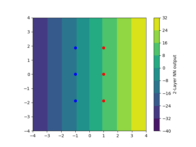
(a) LEFT

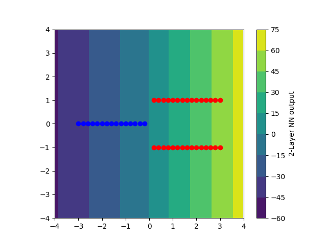
(b) MIDDLE

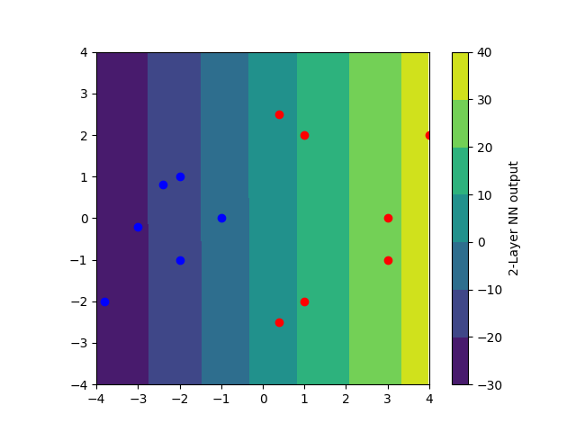
(c) RIGHT

Figure 2: Two-layer Leaky ReLU neural nets converge to functions with linear decision boundary for the examples in Figure 1. The output contours are displayed in colors, and lighter colors mean higher outputs.

I.2 On the Non-branching Starting Point Assumptions

In the proofs of the main theorems we make assumptions regarding the starting point of gradient flow trajectories being non-branching (Assumption 4.6 for the symmetric case and Assumption A.6 for the non-symmetric case). The assumptions address a technical difficulty due to the potential non-uniqueness of gradient flow trajectories on general non-smooth loss functions. The motivations for these assumptions are explained below.

I.2.1 The non-uniqueness of gradient flow trajectories

Gradient flow trajectories are unique on smooth loss functions by the classic theory of ordinary differential equations. In this case, for trajectory defined by $\frac{\textup{{d}}{\bm{\theta}}}{\textup{{d}}t}=-\nabla\mathcal{L}({\bm{\theta}})$, at any point ${\bm{\theta}}_{0}$, if both $\nabla\mathcal{L}({\bm{\theta}}_{0})$ and $\nabla^{2}\mathcal{L}({\bm{\theta}}_{0})$ are continuous, then the trajectory is unique as long as it exists.

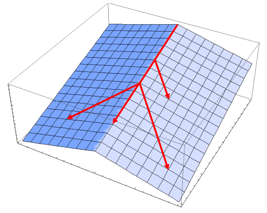
(a) Ridge

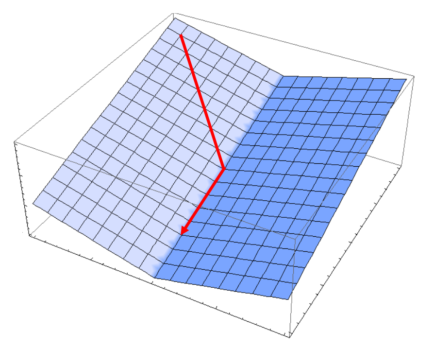
(b) Valley

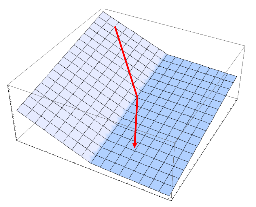
(c) Refraction edge

Figure 3: Gradient flow trajectories behave differently in different landscapes. The trajectory may be non-unique only after arriving at a point on the "ridge".

For the non-smooth case with differential inclusion $\frac{\textup{{d}}{\bm{\theta}}}{\textup{{d}}t}\in-\partial^{\circ}\mathcal{L}({\bm{\theta}})$, when $\mathcal{L}$ is continuous and convex, the Clarke subdifferentials agree with the subdifferentials for convex functions, and gradient flow trajectory is also unique (for instance see Bolte et al. 2010). However, on loss functions that are non-smooth and non-convex, gradient flow may not be unique and the trajectory may branch at non-differentiable points (see Figure 3). When a non-differentiable point is atop a “ridge”, a gradient flow reaching it may go down different slopes next. Then any starting points wherefrom gradient flow can reach such on-the-ridge points are not non-branching starting points as the trajectory is not unique. For instance, with $\mathcal{L}({\bm{\theta}})=-\lvert\langle{\bm{\theta}},{\bm{w}}\rangle\rvert$, then the trajectory with ${\bm{\theta}}(t)=0$ for $t<t_{s}$ and ${\bm{\theta}}(t)=\pm(t-t_{s}){\bm{w}}$ for $t\geq t_{s}$ is a valid gradient flow trajectory for any $t_{s}\geq 0$. On the other hand, when the point is either at the bottom of a “valley” or at a “refraction edge”, the trajectory would not split. Figure 3 sketches in red the possible gradient flow trajectories in different circumstances.

In the case of two-layer Leaky ReLU network dynamics, there are settings where Assumption 4.6 or Assumption A.6 holds. When data points are orthogonally separable (Definition H.1), all starting points are non-branching. In this case, the output of each Leaky ReLU neuron will change monotonically. By the chain rule, for any neuron $k\in[m]$, on any data sample $i\in[n]$,

$$\left<\frac{\textup{{d}}{\bm{w}}_{k}}{\textup{{d}}t},x_{i}\right>\in-\frac{a_{k}}{n}\sum_{j\in[n]}\ell^{\prime}(q_{j}({\bm{\theta}}))y_{j}\phi^{\circ}(\left<{\bm{w}}_{k},{\bm{x}}_{i}\right>)\left<x_{i},x_{j}\right>.$$

Then as $y_{i}y_{j}\left<{\bm{x}}_{i},{\bm{x}}_{j}\right>\geq 0$ by the orthogonally separability, the sign of RHS is controlled by $\mathrm{sgn}(a_{k}y_{i})$. With Theorem B.19, we know each $a_{k}$ does not change its sign along the gradient flow trajectory, and therefore $\left<{\bm{w}}_{k},x_{i}\right>$ changes monotonically. Then following the arguements of the classic theory of ordinary differential equation, by applying Grönwall’s inequality to both intervals $\{t:\left<{\bm{w}}_{k}(t),x_{i}\right>>0\}$ and $\{t:\left<{\bm{w}}_{k}(t),x_{i}\right>\leq 0\}$ we know the trajectory is unique. In this setting all the non-differentiable landscapes resemble the “refraction edges”.

In the general cases, it is a future research direction to find other analyses that can replace the non-branching starting point assumptions, and doing so may deepen our understanding in the trajectory behaviors in non-smooth settings.

Appendix J Additional Experiments

We conducted several additional experiments on synthetic datasets. The goal is to show that 2-layer Leaky ReLU networks actually converges to the max-margin linear classifiers in different settings with moderately small initialization. The results are summarized in Table 1 and Figure 4.

Dataset size	SVM test error	2-Layer neural net test error
10	30.2%	30.5 %
20	19.7%	18.9%
30	17.6%	15.6%
40	8.0%	7.1%
50	6.4%	5.9%
60	6.3%	5.1%
70	7.6%	6.5%
80	3.9%	3.1%
90	6.1%	5.2%
100	2.9%	2.9%

Table 1: Test errors for SVM max-margin linear classifiers and 2-Layer ReLU neural networks are nearly the same across different data size.

Data.

$n=10,20,\cdots,100$ data points are randomly sampled from the standard gaussian distribution $\mathcal{N}(0,{\bm{I}})$ in the space of dimension $d=50$, and are classified with a linear classifier through zero. Then the points are translated mildly away from the classifier to make a small nonzero margin that assists learning.

Model and Training.

We used the two-layer leaky ReLU network with hidden layer width $m=100$ and with bias terms. In out setting the bias term is equivalent to adding an extra dimension of value $0.1$ to all the data points. We trained our model with the gradient descent method from 0.001 times the He initialization [He et al., 2015] and initial learning rate 0.01. The learning rate is raised after interpolation to boost margin increase.

We compare the neural network output with the max-margin linear classfier produced by the support vector machine (SVM) on hinge loss. In Table 1, the test errors are calculated from 10000 test points from the same distribution. In Figure 4, we drawn the decision boundaries for both the SVM max-margin linear classifier and the neural network restricted to a plane passing 0. The results show that the neural network classifier converges to the max-margin linear classfier in our setting.

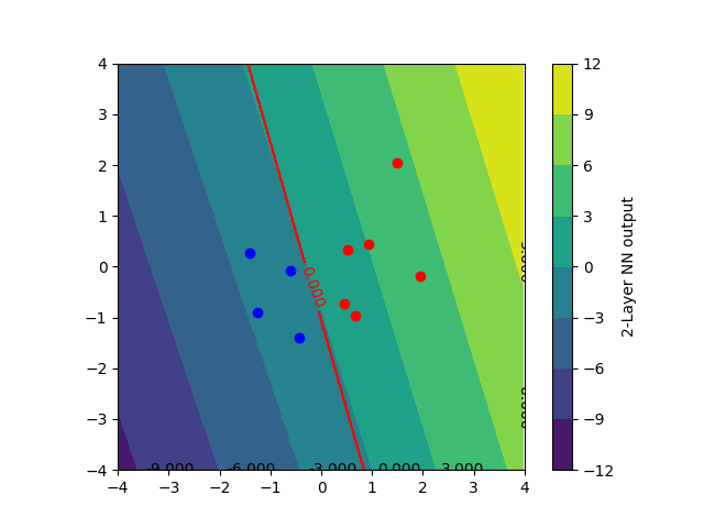
(a) $n=10$

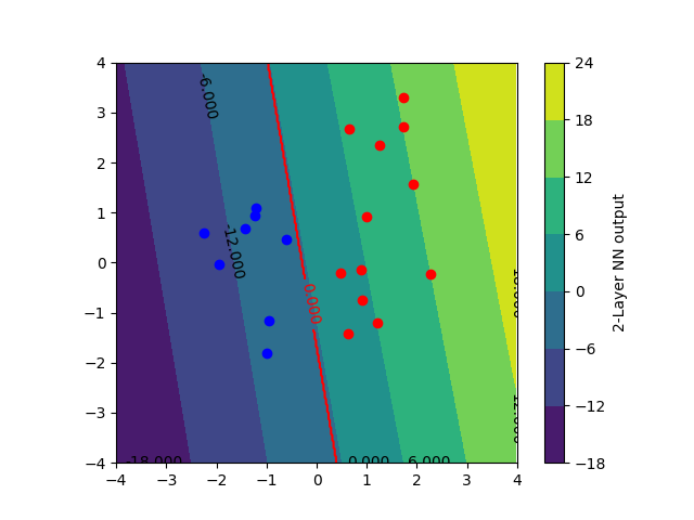
(b) $n=20$

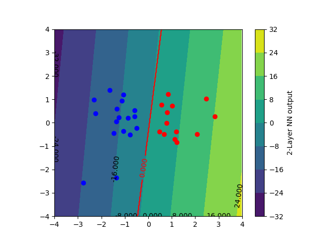
(c) $n=30$

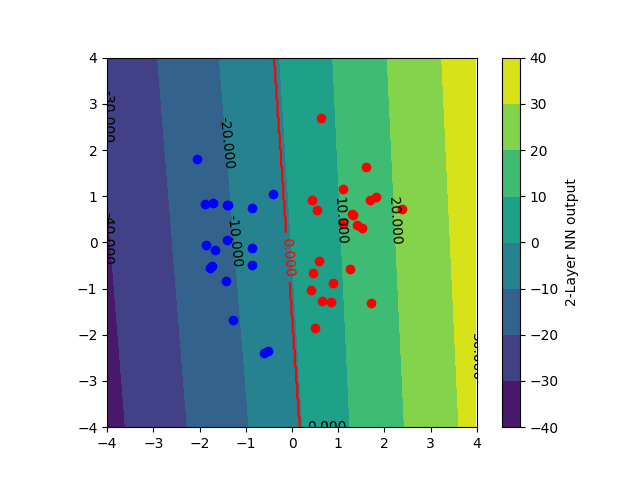
(d) $n=40$

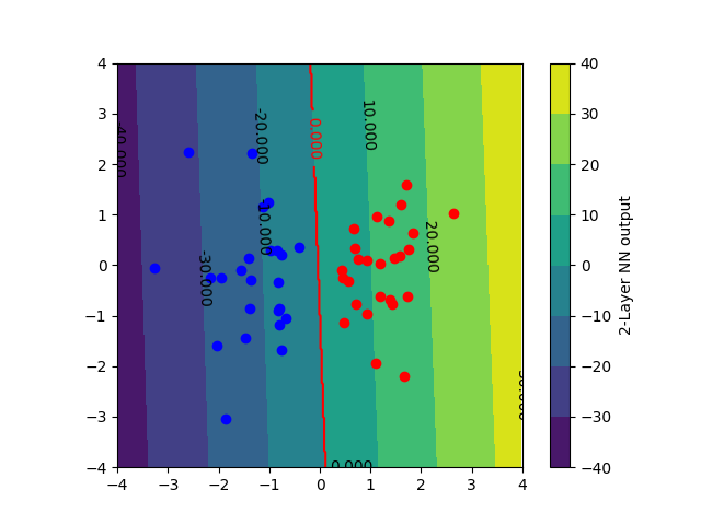
(e) $n=50$

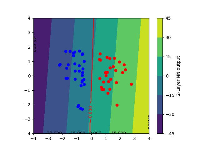
(f) $n=60$

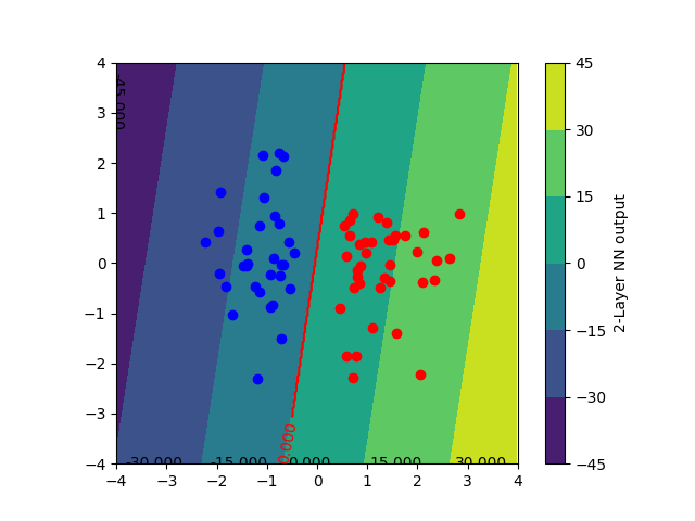
(g) $n=70$

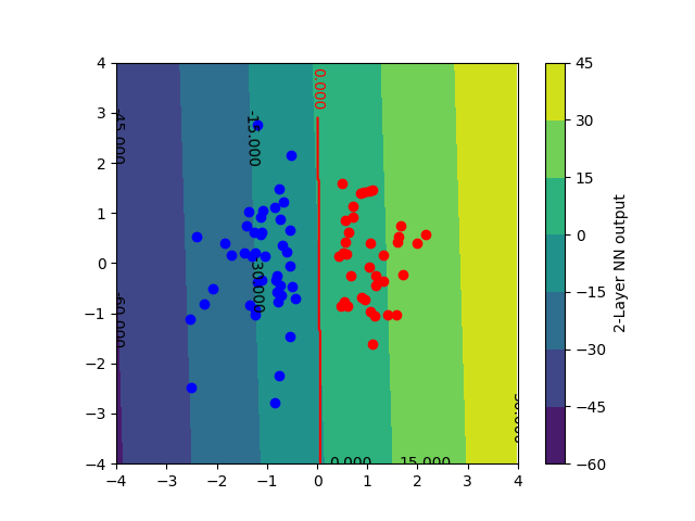
(h) $n=80$

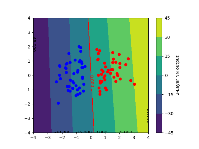
(i) $n=90$

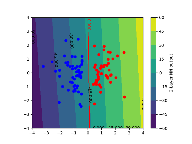
(j) $n=100$

Figure 4: Two-layer Leaky ReLU neural net converges in direction to the SVM max-margin linear classifier. Red and Blue Dots: two classes of data points. Red Lines: the decision boundaries of the SVM max-margin linear classifiers. Background: the contours of two-layer leaky-ReLU neural network outputs. Lighter colors mean higher outputs. The underlying true separator is the vertical line through zero.

References

- Allen-Zhu et al. [2018] Zeyuan Allen-Zhu, Yuanzhi Li, and Yingyu Liang. Learning and generalization in overparameterized neural networks, going beyond two layers, 2018.
- Allen-Zhu et al. [2019] Zeyuan Allen-Zhu, Yuanzhi Li, and Zhao Song. A convergence theory for deep learning via over-parameterization. In Kamalika Chaudhuri and Ruslan Salakhutdinov, editors, Proceedings of the 36th International Conference on Machine Learning, volume 97 of Proceedings of Machine Learning Research, pages 242–252, Long Beach, California, USA, 09–15 Jun 2019. PMLR.
- Arora et al. [2019a] Sanjeev Arora, Nadav Cohen, Wei Hu, and Yuping Luo. Implicit regularization in deep matrix factorization. In H. Wallach, H. Larochelle, A. Beygelzimer, F. d’ Alché-Buc, E. Fox, and R. Garnett, editors, Advances in Neural Information Processing Systems 32, pages 7411–7422. Curran Associates, Inc., 2019a.
- Arora et al. [2019b] Sanjeev Arora, Simon Du, Wei Hu, Zhiyuan Li, and Ruosong Wang. Fine-grained analysis of optimization and generalization for overparameterized two-layer neural networks. In Kamalika Chaudhuri and Ruslan Salakhutdinov, editors, Proceedings of the 36th International Conference on Machine Learning, volume 97 of Proceedings of Machine Learning Research, pages 322–332. PMLR, 09–15 Jun 2019b.
- Bartlett et al. [2017] Peter L Bartlett, Dylan J Foster, and Matus J Telgarsky. Spectrally-normalized margin bounds for neural networks. In I. Guyon, U. V. Luxburg, S. Bengio, H. Wallach, R. Fergus, S. Vishwanathan, and R. Garnett, editors, Advances in Neural Information Processing Systems 30, pages 6240–6249. Curran Associates, Inc., 2017.
- Bolte et al. [2010] Jérôme Bolte, Aris Daniilidis, Olivier Ley, and Laurent Mazet. Characterizations of łojasiewicz inequalities: subgradient flows, talweg, convexity. Transactions of the American Mathematical Society, 362(6):3319–3363, 2010.
- Brutzkus and Globerson [2019] Alon Brutzkus and Amir Globerson. Why do larger models generalize better? A theoretical perspective via the XOR problem. In Kamalika Chaudhuri and Ruslan Salakhutdinov, editors, Proceedings of the 36th International Conference on Machine Learning, volume 97 of Proceedings of Machine Learning Research, pages 822–830. PMLR, 09–15 Jun 2019.
- Brutzkus et al. [2018] Alon Brutzkus, Amir Globerson, Eran Malach, and Shai Shalev-Shwartz. SGD learns over-parameterized networks that provably generalize on linearly separable data. In International Conference on Learning Representations, 2018.
- Chen et al. [2021] Zixiang Chen, Yuan Cao, Difan Zou, and Quanquan Gu. How much over-parameterization is sufficient to learn deep ReLU networks? In International Conference on Learning Representations, 2021.
- Chizat and Bach [2020] Lénaïc Chizat and Francis Bach. Implicit bias of gradient descent for wide two-layer neural networks trained with the logistic loss. In Jacob Abernethy and Shivani Agarwal, editors, Proceedings of Thirty Third Conference on Learning Theory, volume 125 of Proceedings of Machine Learning Research, pages 1305–1338. PMLR, 09–12 Jul 2020.
- Chizat et al. [2019] Lénaïc Chizat, Edouard Oyallon, and Francis Bach. On lazy training in differentiable programming. In H. Wallach, H. Larochelle, A. Beygelzimer, F. d'Alché-Buc, E. Fox, and R. Garnett, editors, Advances in Neural Information Processing Systems 32, pages 2937–2947. Curran Associates, Inc., 2019.
- Clarke et al. [2008] Francis H. Clarke, Yuri S. Ledyaev, Ronald J. Stern, and Peter R. Wolenski. Nonsmooth analysis and control theory, volume 178. Springer Science & Business Media, 2008.
- Clarke [1975] Frank H. Clarke. Generalized gradients and applications. Transactions of the American Mathematical Society, 205:247–262, 1975.
- Coste [2000] Michel Coste. An introduction to o-minimal geometry. Istituti editoriali e poligrafici internazionali Pisa, 2000.
- Davis et al. [2020] Damek Davis, Dmitriy Drusvyatskiy, Sham Kakade, and Jason D. Lee. Stochastic subgradient method converges on tame functions. Foundations of Computational Mathematics, 20(1):119–154, Feb 2020.
- Du et al. [2019a] Simon Du, Jason Lee, Haochuan Li, Liwei Wang, and Xiyu Zhai. Gradient descent finds global minima of deep neural networks. In Kamalika Chaudhuri and Ruslan Salakhutdinov, editors, Proceedings of the 36th International Conference on Machine Learning, volume 97 of Proceedings of Machine Learning Research, pages 1675–1685, Long Beach, California, USA, 09–15 Jun 2019a. PMLR.
- Du et al. [2018] Simon S. Du, Wei Hu, and Jason D. Lee. Algorithmic regularization in learning deep homogeneous models: Layers are automatically balanced. In S. Bengio, H. Wallach, H. Larochelle, K. Grauman, N. Cesa-Bianchi, and R. Garnett, editors, Advances in Neural Information Processing Systems 31, pages 382–393. Curran Associates, Inc., 2018.
- Du et al. [2019b] Simon S. Du, Xiyu Zhai, Barnabas Poczos, and Aarti Singh. Gradient descent provably optimizes over-parameterized neural networks. In International Conference on Learning Representations, 2019b.
- Dutta et al. [2013] Joydeep Dutta, Kalyanmoy Deb, Rupesh Tulshyan, and Ramnik Arora. Approximate KKT points and a proximity measure for termination. Journal of Global Optimization, 56(4):1463–1499, 2013.
- Frei et al. [2021] Spencer Frei, Yuan Cao, and Quanquan Gu. Provable generalization of sgd-trained neural networks of any width in the presence of adversarial label noise. In Marina Meila and Tong Zhang, editors, Proceedings of the 38th International Conference on Machine Learning, volume 139 of Proceedings of Machine Learning Research, pages 3427–3438. PMLR, 18–24 Jul 2021.
- Gidel et al. [2019] Gauthier Gidel, Francis Bach, and Simon Lacoste-Julien. Implicit regularization of discrete gradient dynamics in linear neural networks. In H. Wallach, H. Larochelle, A. Beygelzimer, F. d’ Alché-Buc, E. Fox, and R. Garnett, editors, Advances in Neural Information Processing Systems 32, pages 3196–3206. Curran Associates, Inc., 2019.
- Gissin et al. [2020] Daniel Gissin, Shai Shalev-Shwartz, and Amit Daniely. The implicit bias of depth: How incremental learning drives generalization. In International Conference on Learning Representations, 2020.
- Gunasekar et al. [2018a] Suriya Gunasekar, Jason Lee, Daniel Soudry, and Nathan Srebro. Characterizing implicit bias in terms of optimization geometry. In Jennifer Dy and Andreas Krause, editors, Proceedings of the 35th International Conference on Machine Learning, volume 80 of Proceedings of Machine Learning Research, pages 1832–1841, Stockholmsmässan, Stockholm Sweden, 10–15 Jul 2018a. PMLR.
- Gunasekar et al. [2018b] Suriya Gunasekar, Jason D Lee, Daniel Soudry, and Nati Srebro. Implicit bias of gradient descent on linear convolutional networks. In S. Bengio, H. Wallach, H. Larochelle, K. Grauman, N. Cesa-Bianchi, and R. Garnett, editors, Advances in Neural Information Processing Systems 31, pages 9482–9491. Curran Associates, Inc., 2018b.
- He et al. [2015] Kaiming He, Xiangyu Zhang, Shaoqing Ren, and Jian Sun. Delving deep into rectifiers: Surpassing human-level performance on ImageNet classification. In The IEEE International Conference on Computer Vision (ICCV), December 2015.
- Hu et al. [2020] Wei Hu, Lechao Xiao, Ben Adlam, and Jeffrey Pennington. The surprising simplicity of the early-time learning dynamics of neural networks. In H. Larochelle, M. Ranzato, R. Hadsell, M. F. Balcan, and H. Lin, editors, Advances in Neural Information Processing Systems, volume 33, pages 17116–17128. Curran Associates, Inc., 2020.
- Jacot et al. [2018] Arthur Jacot, Franck Gabriel, and Clement Hongler. Neural tangent kernel: Convergence and generalization in neural networks. In S. Bengio, H. Wallach, H. Larochelle, K. Grauman, N. Cesa-Bianchi, and R. Garnett, editors, Advances in Neural Information Processing Systems 31, pages 8571–8580. Curran Associates, Inc., 2018.
- Ji and Telgarsky [2018] Ziwei Ji and Matus Telgarsky. Risk and parameter convergence of logistic regression. arXiv preprint arXiv:1803.07300, 2018.
- Ji and Telgarsky [2019a] Ziwei Ji and Matus Telgarsky. Gradient descent aligns the layers of deep linear networks. In International Conference on Learning Representations, 2019a.
- Ji and Telgarsky [2019b] Ziwei Ji and Matus Telgarsky. The implicit bias of gradient descent on nonseparable data. In Alina Beygelzimer and Daniel Hsu, editors, Proceedings of the Thirty-Second Conference on Learning Theory, volume 99 of Proceedings of Machine Learning Research, pages 1772–1798, Phoenix, USA, 25–28 Jun 2019b. PMLR.
- Ji and Telgarsky [2020a] Ziwei Ji and Matus Telgarsky. Directional convergence and alignment in deep learning. In H. Larochelle, M. Ranzato, R. Hadsell, M. F. Balcan, and H. Lin, editors, Advances in Neural Information Processing Systems, volume 33, pages 17176–17186. Curran Associates, Inc., 2020a.
- Ji and Telgarsky [2020b] Ziwei Ji and Matus Telgarsky. Polylogarithmic width suffices for gradient descent to achieve arbitrarily small test error with shallow relu networks. In International Conference on Learning Representations, 2020b.
- Jiang et al. [2020] Yiding Jiang, Behnam Neyshabur, Hossein Mobahi, Dilip Krishnan, and Samy Bengio. Fantastic generalization measures and where to find them. In International Conference on Learning Representations, 2020.
- Kalimeris et al. [2019] Dimitris Kalimeris, Gal Kaplun, Preetum Nakkiran, Benjamin Edelman, Tristan Yang, Boaz Barak, and Haofeng Zhang. SGD on neural networks learns functions of increasing complexity. In H. Wallach, H. Larochelle, A. Beygelzimer, F. d'Alché-Buc, E. Fox, and R. Garnett, editors, Advances in Neural Information Processing Systems, volume 32. Curran Associates, Inc., 2019.
- Li et al. [2018] Yuanzhi Li, Tengyu Ma, and Hongyang Zhang. Algorithmic regularization in over-parameterized matrix sensing and neural networks with quadratic activations. In Sébastien Bubeck, Vianney Perchet, and Philippe Rigollet, editors, Proceedings of the 31st Conference On Learning Theory, volume 75 of Proceedings of Machine Learning Research, pages 2–47. PMLR, 06–09 Jul 2018.
- Li et al. [2021] Zhiyuan Li, Yuping Luo, and Kaifeng Lyu. Towards resolving the implicit bias of gradient descent for matrix factorization: Greedy low-rank learning. In International Conference on Learning Representations, 2021.
- Luo et al. [2021] Tao Luo, Zhi-Qin John Xu, Zheng Ma, and Yaoyu Zhang. Phase diagram for two-layer relu neural networks at infinite-width limit. Journal of Machine Learning Research, 22(71):1–47, 2021.
- Lyu and Li [2020] Kaifeng Lyu and Jian Li. Gradient descent maximizes the margin of homogeneous neural networks. In International Conference on Learning Representations, 2020.
- Maas et al. [2013] Andrew L. Maas, Awni Y. Hannun, and Andrew Y. Ng. Rectifier nonlinearities improve neural network acoustic models. In ICML Workshop on Deep Learning for Audio, Speech and Language Processing, 2013.
- Maennel et al. [2018] Hartmut Maennel, Olivier Bousquet, and Sylvain Gelly. Gradient descent quantizes relu network features. arXiv preprint arXiv:1803.08367, 2018.
- Mehta et al. [2021] Harsh Mehta, Ashok Cutkosky, and Behnam Neyshabur. Extreme memorization via scale of initialization. In International Conference on Learning Representations, 2021.
- Moroshko et al. [2020] Edward Moroshko, Blake E Woodworth, Suriya Gunasekar, Jason D Lee, Nati Srebro, and Daniel Soudry. Implicit bias in deep linear classification: Initialization scale vs training accuracy. In H. Larochelle, M. Ranzato, R. Hadsell, M. F. Balcan, and H. Lin, editors, Advances in Neural Information Processing Systems, volume 33, pages 22182–22193. Curran Associates, Inc., 2020.
- Nacson et al. [2019a] Mor Shpigel Nacson, Jason Lee, Suriya Gunasekar, Pedro Henrique Pamplona Savarese, Nathan Srebro, and Daniel Soudry. Convergence of gradient descent on separable data. In Kamalika Chaudhuri and Masashi Sugiyama, editors, Proceedings of Machine Learning Research, volume 89 of Proceedings of Machine Learning Research, pages 3420–3428. PMLR, 16–18 Apr 2019a.
- Nacson et al. [2019b] Mor Shpigel Nacson, Nathan Srebro, and Daniel Soudry. Stochastic gradient descent on separable data: Exact convergence with a fixed learning rate. In Kamalika Chaudhuri and Masashi Sugiyama, editors, Proceedings of Machine Learning Research, volume 89 of Proceedings of Machine Learning Research, pages 3051–3059. PMLR, 16–18 Apr 2019b.
- Neyshabur et al. [2018] Behnam Neyshabur, Srinadh Bhojanapalli, and Nathan Srebro. A PAC-bayesian approach to spectrally-normalized margin bounds for neural networks. In International Conference on Learning Representations, 2018.
- Pellegrini and Biroli [2020] Franco Pellegrini and Giulio Biroli. An analytic theory of shallow networks dynamics for hinge loss classification. In H. Larochelle, M. Ranzato, R. Hadsell, M. F. Balcan, and H. Lin, editors, Advances in Neural Information Processing Systems, volume 33, pages 5356–5367. Curran Associates, Inc., 2020.
- Phuong and Lampert [2021] Mary Phuong and Christoph H Lampert. The inductive bias of ReLU networks on orthogonally separable data. In International Conference on Learning Representations, 2021.
- Razin et al. [2021] Noam Razin, Asaf Maman, and Nadav Cohen. Implicit regularization in tensor factorization. In Marina Meila and Tong Zhang, editors, Proceedings of the 38th International Conference on Machine Learning, volume 139 of Proceedings of Machine Learning Research, pages 8913–8924. PMLR, 18–24 Jul 2021.
- Sarussi et al. [2021] Roei Sarussi, Alon Brutzkus, and Amir Globerson. Towards understanding learning in neural networks with linear teachers. In Marina Meila and Tong Zhang, editors, Proceedings of the 38th International Conference on Machine Learning, volume 139 of Proceedings of Machine Learning Research, pages 9313–9322. PMLR, 18–24 Jul 2021.
- Shah et al. [2020] Harshay Shah, Kaustav Tamuly, Aditi Raghunathan, Prateek Jain, and Praneeth Netrapalli. The pitfalls of simplicity bias in neural networks. In H. Larochelle, M. Ranzato, R. Hadsell, M. F. Balcan, and H. Lin, editors, Advances in Neural Information Processing Systems, volume 33, pages 9573–9585. Curran Associates, Inc., 2020.
- Soudry et al. [2018a] Daniel Soudry, Elad Hoffer, Mor Shpigel Nacson, Suriya Gunasekar, and Nathan Srebro. The implicit bias of gradient descent on separable data. Journal of Machine Learning Research, 19(70):1–57, 2018a.
- Soudry et al. [2018b] Daniel Soudry, Elad Hoffer, and Nathan Srebro. The implicit bias of gradient descent on separable data. In International Conference on Learning Representations, 2018b.
- Williams et al. [2019] Francis Williams, Matthew Trager, Daniele Panozzo, Claudio Silva, Denis Zorin, and Joan Bruna. Gradient dynamics of shallow univariate relu networks. In H. Wallach, H. Larochelle, A. Beygelzimer, F. d'Alché-Buc, E. Fox, and R. Garnett, editors, Advances in Neural Information Processing Systems, volume 32. Curran Associates, Inc., 2019.
- Woodworth et al. [2020] Blake Woodworth, Suriya Gunasekar, Jason D. Lee, Edward Moroshko, Pedro Savarese, Itay Golan, Daniel Soudry, and Nathan Srebro. Kernel and rich regimes in overparametrized models. In Jacob Abernethy and Shivani Agarwal, editors, Proceedings of Thirty Third Conference on Learning Theory, volume 125 of Proceedings of Machine Learning Research, pages 3635–3673. PMLR, 09–12 Jul 2020.
- Xu et al. [2021] Zhi-Qin John Xu, Hanxu Zhou, Tao Luo, and Yaoyu Zhang. Towards understanding the condensation of two-layer neural networks at initial training. arXiv preprint arXiv:2105.11686, 2021.
- Zhang et al. [2017] Chiyuan Zhang, Samy Bengio, Moritz Hardt, Benjamin Recht, and Oriol Vinyals. Understanding deep learning requires rethinking generalization. In International Conference on Learning Representations, 2017.
- Zou et al. [2018] Difan Zou, Yuan Cao, Dongruo Zhou, and Quanquan Gu. Stochastic gradient descent optimizes over-parameterized deep relu networks. arXiv preprint arXiv:1811.08888, 2018.