An interface-tracking space-time hybridizable/embedded discontinuous Galerkin method for nonlinear free-surface flows

Abstract

We present a compatible space-time hybridizable/embedded discontinuous Galerkin discretization for nonlinear free-surface waves. We pose this problem in a two-fluid (liquid and gas) domain and use a time-dependent level-set function to identify the sharp interface between the two fluids. The incompressible two-fluid equations are discretized by an exactly mass conserving space-time hybridizable discontinuous Galerkin method while the level-set equation is discretized by a space-time embedded discontinuous Galerkin method. Different from alternative discontinuous Galerkin methods is that the embedded discontinuous Galerkin method results in a continuous approximation of the interface. This, in combination with the space-time framework, results in an interface-tracking method without resorting to smoothing techniques or additional mesh stabilization terms.

1 Introduction

Free-surface problems arise in many real-world applications such as in the design of ships and offshore structures, modeling of tsunamis, and dam breaking. Mathematically, nonlinear free-surface wave problems are described by a set of partial differential equations that govern the movement of the fluid together with certain nonlinear boundary conditions that describe the free-surface. Modeling such problems is challenging because the boundary of the computational domain depends on the solution of the problem. This implies that there is a strong coupling between the fluid and the free-surface, and the domain must be continuously updated to track the changes in the free-surface.

Discontinuous Galerkin (DG) finite element methods posses excellent conservation and stability properties, and provide higher-order accurate approximate solutions. DG methods are therefore well suited for the spatial discretization of free-surface problems. Hybridizable discontinuous Galerkin (HDG) methods possess the same properties as the DG method, but at a lower computational cost [1, 2, 3]. This is achieved by reducing the number of globally coupled degrees-of-freedom. In HDG methods, so-called facet variables are introduced that live only on the facets of the mesh. The HDG method is then constructed such that communication between element unknowns is done only through this facet variable. This construction allows for static condensation which significantly reduces the total number of globally coupled degrees-of-freedom; it is possible to eliminate the element degrees-of-freedom and solve a linear system only for the facet degrees-of-freedom. Given the facet degrees-of-freedom, the element variables can be reconstructed element-wise. For incompressible flows the HDG method can be constructed such that the approximate velocity is $H(\text{div})$-conforming and point-wise divergence free on the elements (see for example [4, 5, 6]). We remark that to lower the number of globally coupled degrees-of-freedom even further one may impose that the facet variables are continuous between facets resulting in the embedded discontinuous Galerkin (EDG) method [7, 8, 9].

Free-surface problems can be viewed as two-fluid, e.g. liquid and gas, flow problems and so level-set methods can be used for their discretization. Level-set methods were first introduced in [10] and have since been used for multi-phase flows [11, 12], and for free-surface flows [13, 14, 15]. Using the two-fluid approach, the fluid equations are solved in a domain that contains both liquid and gas phases. In this set-up, the viscosity and density are defined as piece-wise constant functions that are discontinuous across the liquid-gas interface. A level-set function, which satisfies an advection equation where the advection field is the velocity of the fluid, is defined such that it is positive in one of the fluids and negative in the other. The zero level-set then corresponds to the interface between the two fluids. Traditionally, when using level-set methods, the mesh remains fixed throughout the computation. This results in there being mesh elements in which the density and viscosity take two different values. To handle this, the density and viscosity of both fluids are smoothed throughout a band around the interface. This results in non-physical fluid properties, and introduces an extra parameter (the thickness of the band) in the discretization of the problem. Instead, in this paper we consider an interface-tracking method by solving the time dependent advection equation for the level-set function and moving the mesh to fit the zero level-set. Since every mesh element will belong to only one of the fluids’ domains, no smoothing is necessary of the density and viscosity. Two well-known approaches to handle moving meshes are the Arbitrary Lagrangian-Eulerian (ALE) approach [16, 17, 18] and the space-time approach [19, 20, 21, 22, 23]. In this paper we consider the space-time framework.

We describe the two-fluid model and its space-time EDG/HDG discretization in, respectively, sections 2 and 3. The discretization of the incompressible two-fluid model is based on the space-time HDG method developed in [24, 25] for the single-phase incompressible Navier–Stokes equations. This discretization, like the ALE discretizations in [17, 18], is exactly mass conserving, even on moving meshes. For the level-set equation, however, we do not use HDG. A continuous representation of the zero level-set is required to fit the mesh to the interface between the two fluids. The HDG method, however, results in a discontinuous polynomial approximation of the level-set function and so a smoothing technique would be required to obtain a continuous approximation of the interface. It was shown in [26], however, that such smoothing may lead to instabilities unless the discretization is modified by adding extra stabilization terms. Instead, we propose to use a space-time EDG discretization for the level-set equation. The EDG method directly results in a continuous approximation to the free-surface resulting in a straightforward approach to update the mesh. In section 3 we furthermore show that the space-time HDG method for the incompressible two-fluid model is compatible with the space-time EDG method for the level-set equation, i.e., that the space-time EDG method is able to preserve the constant solution. As discussed in [27], for discontinuous Galerkin methods compatibility is a stronger statement than local conservation of the flow field. It was furthermore shown in [27] that if a method is not compatible it may produce erroneous solutions. In section 4 we describe the solution algorithm while numerical simulations in section 5 demonstrate optimal rates of convergence and that our discretization is energy-stable under mesh movement. We furthermore apply the discretization to simulate sloshing in a tank and flow past a submerged obstacle. Conclusions are drawn in section 6.

2 The space-time incompressible two-fluid flow model

Let us consider a bounded domain $\Omega\subset\mathbb{R}^{2}$ and let $I=(0,t_{N}]$ denote our time interval of interest. We then introduce a space-time domain by $\mathcal{E}\mathrel{\mathop{\mathchar 58\relax}}=\Omega\times I\subset\mathbb{R}^{3}$. We will assume that the space-time domain $\mathcal{E}$ is divided into two non-overlapping polygonal regions, $\mathcal{E}_{\ell}$ and $\mathcal{E}_{g}$, such that $\mathcal{E}=\mathcal{E}_{\ell}\cup\mathcal{E}_{g}$. In what follows, $\mathcal{E}_{\ell}$ and $\mathcal{E}_{g}$ represent, respectively, the liquid and gas regions of the space-time domain. We denote the liquid and gas regions at a particular time level $\tau$ by $\Omega_{\ell}(\tau)\mathrel{\mathop{\mathchar 58\relax}}=\mathinner{\{(x,t)\in\mathcal{E}_{\ell}\ \mathrel{\mathop{\mathchar 58\relax}}\ t=\tau\}}$ and $\Omega_{g}(\tau)\mathrel{\mathop{\mathchar 58\relax}}=\mathinner{\{(x,t)\in\mathcal{E}_{g}\ \mathrel{\mathop{\mathchar 58\relax}}\ t=\tau\}}$. Here $x=(x_{1},x_{2})$. Note that the spatial domains $\Omega_{\ell}$ and $\Omega_{g}$ are time-dependent.

The space-time interface between the liquid and gas regions is defined as

$$\mathcal{S}\mathrel{\mathop{\mathchar 58\relax}}=\mathinner{\bigl{\{}(x,t)\in\mathcal{E}\ \mathrel{\mathop{\mathchar 58\relax}}\ x_{2}=\zeta(x_{1},t)\bigr{\}}},$$ (1)

where $\zeta(x_{1},t)$ is the wave height. We will denote the interface at time level $\tau$ by $\Gamma_{s}(\tau)\mathrel{\mathop{\mathchar 58\relax}}=\mathinner{\{(x,t)\in\mathcal{S}\ \mathrel{\mathop{\mathchar 58\relax}}\ t=\tau\}}$. A plot of the domain at some time level $\tau$ is given in fig. 1.

Figure 1: A description of the two-fluid flow domain $\Omega\subset\mathbb{R}^{2}$ at time $t=\tau$.

The position of the interface eq. 1 is not known a priori. To find its position we introduce the level-set function $\phi(x,t)=\zeta(x_{1},t)-x_{2}$ and the Heaviside function $H(\phi)$ which is defined by

$$H(\phi)=\begin{cases}1&\text{if }\phi>0,\\ 0&\text{if }\phi<0.\end{cases}$$

We note that the interface corresponds to the zero level-set, $\phi=0$.

Let $k$ be a subscript to denote a liquid ($k=\ell$) or a gas ($k=g$) property. Then given the dynamic viscosities $\mu_{k}\in\mathbb{R}^{+}$, the constant densities $\rho_{k}\in\mathbb{R}^{+}$, and the constant acceleration due to gravity $g$, the space-time formulation of the incompressible two-fluid flow model for the velocity $u\mathrel{\mathop{\mathchar 58\relax}}\mathcal{E}\to\mathbb{R}^{2}$ and pressure $p\mathrel{\mathop{\mathchar 58\relax}}\mathcal{E}\to\mathbb{R}$ is given by

$$\rho\mathinner{\bigl{(}\partial_{t}u+u\cdot\nabla u\bigr{)}}+\nabla p-\nabla\cdot 2\mu\varepsilon(u) =-\rho ge_{2} \text{ in }\mathcal{E},$$ (2a)

$$\nabla\cdot u =0 \text{ in }\mathcal{E},$$ (2b)

$$\partial_{t}\phi+u\cdot\nabla\phi =0 \text{ in }\mathcal{E},$$ (2c)

where $\varepsilon(u)\mathrel{\mathop{\mathchar 58\relax}}=(\nabla u+(\nabla u)^{T})/2$ is the symmetric gradient, $e_{2}$ is the unit vector in the $x_{2}$-direction and

$$u =u_{g}+(u_{\ell}-u_{g})H(\phi), p =p_{g}+(p_{\ell}-p_{g})H(\phi),$$ (3a)

$$\rho =\rho_{g}+(\rho_{\ell}-\rho_{g})H(\phi), \mu =\mu_{g}+(\mu_{\ell}-\mu_{g})H(\phi).$$ (3b)

Let $\Omega_{0}\mathrel{\mathop{\mathchar 58\relax}}=\mathinner{\{(x,t)\in\partial\mathcal{E}\ \mathrel{\mathop{\mathchar 58\relax}}\ t=0\}}$ and similarly $\Omega_{N}\mathrel{\mathop{\mathchar 58\relax}}=\mathinner{\{(x,t)\in\partial\mathcal{E}\ \mathrel{\mathop{\mathchar 58\relax}}\ t=t_{N}\}}$. Then the boundary of the space-time domain $\mathcal{E}$ is partitioned such that $\partial\mathcal{E}=\partial\mathcal{E}^{D}\cup\partial\mathcal{E}^{N}\cup\Omega_{0}\cup\Omega_{N}$, where there is no overlap between the four sets. Here, $\partial\mathcal{E}^{D}$ and $\partial\mathcal{E}^{N}$ denote, respectively, the Dirichlet and Neumann parts of the space-time boundary. The space-time outward unit normal vector to $\partial\mathcal{E}$ is denoted by $(n_{t},n)$, with $n_{t}\in\mathbb{R}$ the temporal component and $n\in\mathbb{R}^{2}$ the spatial component. We define the inflow boundary $\partial\mathcal{E}^{-}$ as the portion of $\partial\mathcal{E}^{N}$ on which $n_{t}+u\cdot n<0$. The outflow boundary is then defined as $\partial\mathcal{E}^{+}\mathrel{\mathop{\mathchar 58\relax}}=\partial\mathcal{E}^{N}\backslash\partial\mathcal{E}^{-}$. We prescribe the following boundary and initial conditions:

$$u =0 \text{on }\partial\mathcal{E}^{D},$$ (4a)

$$\rho\mathinner{[n_{t}+u\cdot n-\max\mathinner{(n_{t}+u\cdot n,0)}]}u+\mathinner{(p\mathbb{I}-2\mu\varepsilon(u))}n =f \text{on }\partial\mathcal{E}^{N},$$ (4b)

$$u(x,0) =u_{0}(x) \text{in }\Omega_{0},$$ (4c)

$$-(n_{t}+u\cdot n)\phi =r \text{on }\partial\mathcal{E}^{-},$$ (4d)

$$\phi(x,0) =\phi_{0}(x) \text{in }\Omega_{0},$$ (4e)

where the boundary data $f\mathrel{\mathop{\mathchar 58\relax}}\partial\mathcal{E}^{N}\to\mathbb{R}^{d}$ and $r\mathrel{\mathop{\mathchar 58\relax}}\partial\mathcal{E}^{-}\to\mathbb{R}$, and the divergence-free initial condition $u_{0}\mathrel{\mathop{\mathchar 58\relax}}\Omega_{0}\to\mathbb{R}^{d}$ are given. Furthermore, $\phi_{0}(x)\mathrel{\mathop{\mathchar 58\relax}}=\zeta_{0}(x_{1})-x_{2}$ with $\zeta_{0}(x_{1})$ the given initial wave height.

We remark that the two-fluid problem assumes continuity of the velocity and of the diffusive flux across the interface $\mathcal{S}$, i.e.,

$$u_{\ell} =u_{g} \text{on }\mathcal{S},$$ (5a)

$$\mathinner{(p_{\ell}\mathbb{I}-2\mu_{\ell}\varepsilon(u_{\ell}))}n_{s} =\mathinner{(p_{g}\mathbb{I}-2\mu_{g}\varepsilon(u_{g}))}n_{s} \text{on }\mathcal{S},$$ (5b)

where $n_{s}$ is the normal vector on the interface $\Gamma_{s}(t)$ pointing outwards from $\Omega_{\ell}(t)$.

3 The space-time hybridizable/embedded discontinuous Galerkin method

In this section we will introduce the space-time discretization for the two-fluid problem eqs. 2 and 4. In particular we will introduce a space-time hybridizable discontinuous Galerkin (HDG) for the momentum and mass eqs. 2a and 2b coupled to a space-time embedded discontinuous Galerkin (EDG) discretization of the level-set equation eq. 2c.

3.1 Space-time notation

We will use notation similar to, for example, [25]. For this we first partition the time interval $I$ into time levels $0=t_{0}<t_{1}<t_{2}<\ldots<t_{N}$ and denote the $n^{\text{th}}$ time interval by $I_{n}=(t_{n},t_{n+1})$. A ‘time-step’ is defined as the length of a time interval, i.e., $\Delta t=t_{n+1}-t_{n}$. Next, we define the $n^{\text{th}}$ space-time slab as $\mathcal{E}^{n}\mathrel{\mathop{\mathchar 58\relax}}=\mathcal{E}\cap\mathinner{\left(I_{n}\times\mathbb{R}^{2}\right)}$, we define the spatial domain at time level $t_{n}$ as $\Omega_{n}\mathrel{\mathop{\mathchar 58\relax}}=\mathinner{\{(x,t)\in\mathcal{E}\mathrel{\mathop{\mathchar 58\relax}}t=t_{n}\}}$, and note that the boundary of a space-time slab, denoted by $\partial\mathcal{E}^{n}$, can be divided into $\Omega_{n}$, $\Omega_{n+1}$, and $\mathcal{Q}_{\mathcal{E}}^{n}\mathrel{\mathop{\mathchar 58\relax}}=\partial\mathcal{E}^{n}\backslash\mathinner{\left(\Omega_{n+1}\cup\Omega_{n}\right)}$.

Following [24, 25] we consider a tetrahedral space-time mesh which is constructed as follows. First, the triangular spatial mesh of $\Omega_{n}$ is extruded to the new time level $t_{n+1}$ according to the domain deformation prescribed by the wave height. (Note that the wave height is not known a priori and so, as we will describe in section 4, an iterative procedure is used to find the final approximation to the domain at time level $t_{n+1}$.) Each element of this prismatic space-time mesh is then subdivided into three tetrahedrons. We denote the space-time triangulation in the space-time slab $\mathcal{E}^{n}$ by $\mathcal{T}^{n}\mathrel{\mathop{\mathchar 58\relax}}=\mathinner{\{\mathcal{K}\}}$. The space-time elements $\mathcal{K}\in\mathcal{T}^{n}$ that lie in the liquid region of the space-time slab form the triangulation $\mathcal{T}^{n}_{\ell}$. $\mathcal{T}^{n}_{g}$ is defined similarly but for the gas region. The triangulation of the whole space-time domain $\mathcal{E}$ is denoted by $\mathcal{T}\mathrel{\mathop{\mathchar 58\relax}}=\cup_{n}\mathcal{T}^{n}$.

The boundary of a space-time tetrahedron $\mathcal{K}_{j}\in\mathcal{T}^{n}$ is denoted by $\partial\mathcal{K}_{j}$ and the outward unit space-time normal vector on the boundary of $\mathcal{K}_{j}\in\mathcal{T}^{n}$ is given by $(n_{t}^{\mathcal{K}_{j}},n^{\mathcal{K}_{j}})$. The boundary $\partial\mathcal{K}_{j}$ consists of at most one face that belongs to a time level (on which $\mathinner{\lvert n_{t}^{\mathcal{K}_{j}}\rvert}=1$). We denote this face by $K_{j}^{n}$ if $n_{t}^{\mathcal{K}_{j}}=-1$ and by $K_{j}^{n+1}$ if $n_{t}^{\mathcal{K}_{j}}=1$. The remaining faces of $\partial\mathcal{K}_{j}$ are denoted by $\mathcal{Q}_{\mathcal{K}_{j}}^{n}\mathrel{\mathop{\mathchar 58\relax}}=\partial\mathcal{K}_{j}\backslash K_{j}^{n}$ or $\mathcal{Q}_{\mathcal{K}_{j}}^{n}\mathrel{\mathop{\mathchar 58\relax}}=\partial\mathcal{K}_{j}\backslash K_{j}^{n+1}$. Note that the space-time normal on $\mathcal{Q}_{\mathcal{K}_{j}}^{n}$ depends on the grid velocity $v_{g}\in\mathbb{R}^{2}$ as follows: $n_{t}^{\mathcal{K}_{j}}=-v_{g}\cdot n$. This relation allows to switch between a space-time formulation and an arbitrary Lagrangian Eulerian (ALE) formulation (see, e.g., [28]). In the remainder of this article, to simplify notation, we drop the sub- and superscript when referring to the space-time normal vector and the space-time cell wherever no confusion will occur.

In a space-time slab $\mathcal{E}^{n}$, the set of all faces for which $\mathinner{\lvert n_{t}\rvert}\neq 1$ is denoted by $\mathcal{F}^{n}$ while the union of these faces is denoted by $\Gamma^{n}$. By $\mathcal{F}_{\mathcal{S}}^{n}$ we denote all the faces in $\mathcal{F}^{n}$ that lie on the interface $\mathcal{S}$. Similarly, the set of all faces in $\mathcal{F}^{n}$ that lie on the boundary of the space-time domain is denoted by $\mathcal{F}^{n}_{B}$. The remaining set of (interior) faces is denoted by $\mathcal{F}_{I}^{n}$. Then $\mathcal{F}^{n}=\mathcal{F}_{I}^{n}\cup\mathcal{F}_{\mathcal{S}}^{n}\cup\mathcal{F}_{B}^{n}$. Furthermore, we will denote the set of faces that lie on a Neumann boundary, $\partial\mathcal{E}^{N}\cap\partial\mathcal{E}^{n}$, by $\mathcal{F}_{N}^{n}$.

On each space-time slab $\mathcal{E}^{n}$ we consider the following discontinuous finite element spaces on $\mathcal{T}^{n}$:

$$V_{h}^{n} \mathrel{\mathop{\mathchar 58\relax}}=\mathinner{\bigl{\{}v_{h}\in\mathinner{[L^{2}(\mathcal{T}^{n})]}^{2}\,\mathrel{\mathop{\mathchar 58\relax}}v_{h}|_{\mathcal{K}}\in\mathinner{\bigl{[}P^{k}(\mathcal{K})\bigr{]}}^{2},\,\forall\mathcal{K}\in\mathcal{T}^{n}\bigr{\}}},$$ (6a)

$$Q_{h}^{n} \mathrel{\mathop{\mathchar 58\relax}}=\mathinner{\bigl{\{}q_{h}\in L^{2}(\mathcal{T}^{n})\mathrel{\mathop{\mathchar 58\relax}}q_{h}|_{\mathcal{K}}\in P^{k-1}(\mathcal{K}),\,\forall\mathcal{K}\in\mathcal{T}^{n}\bigr{\}}},$$ (6b)

$$M_{h}^{n} \mathrel{\mathop{\mathchar 58\relax}}=\mathinner{\bigl{\{}m_{h}\in L^{2}(\mathcal{T}^{n})\mathrel{\mathop{\mathchar 58\relax}}m_{h}|_{\mathcal{K}}\in P^{k}(\mathcal{K}),\,\forall\mathcal{K}\in\mathcal{T}^{n}\bigr{\}}},$$ (6c)

where $P^{l}(D)$ denotes the space of polynomials of degree $l$ on a domain $D$. Additionally, we consider the following facet finite element spaces:

$$\bar{V}_{h}^{n} \mathrel{\mathop{\mathchar 58\relax}}=\mathinner{\bigl{\{}\bar{v}_{h}\in\mathinner{[L^{2}(\mathcal{F}^{n})]}^{2}\,\mathrel{\mathop{\mathchar 58\relax}}\bar{v}_{h}|_{\mathcal{F}}\in\mathinner{[P^{k}(\mathcal{F})]}^{2},\,\forall\mathcal{F}\in\mathcal{F}^{n},\bar{v}_{h}=0\text{ on }\partial\mathcal{E}^{D}\cap\partial\mathcal{E}^{n}\bigr{\}}},$$ (7a)

$$\bar{Q}_{h}^{n} \mathrel{\mathop{\mathchar 58\relax}}=\mathinner{\bigl{\{}\bar{q}_{h}\in L^{2}(\mathcal{F}^{n})\mathrel{\mathop{\mathchar 58\relax}}\bar{q}_{h}|_{\mathcal{F}}\in P^{k}(\mathcal{F}),\,\forall\mathcal{F}\in\mathcal{F}^{n}\bigr{\}}},$$ (7b)

$$\bar{M}_{h}^{n} \mathrel{\mathop{\mathchar 58\relax}}=\mathinner{\bigl{\{}\bar{m}_{h}\in L^{2}(\mathcal{F}^{n})\mathrel{\mathop{\mathchar 58\relax}}\bar{m}_{h}|_{\mathcal{F}}\in P^{k}(\mathcal{F}),\,\forall\mathcal{F}\in\mathcal{F}^{n}\bigr{\}}}\cap C(\Gamma^{n}).$$ (7c)

Note that the facet velocity field in $\bar{V}_{h}^{n}$ and facet pressure field in $\bar{Q}_{h}^{n}$ are discontinuous while the facet level-set field in $\bar{M}_{h}^{n}$ is continuous. To simplify the notation, we introduce $X_{h}^{v,n}\mathrel{\mathop{\mathchar 58\relax}}=V_{h}^{n}\times\bar{V}_{h}^{n}$, $X_{h}^{q,n}=Q_{h}^{n}\times\bar{Q}_{h}^{n}$, $X_{h}^{n}=X_{h}^{v,n}\times X_{h}^{q,n}$, and $X_{h}^{m,n}=M_{h}^{n}\times\bar{M}_{h}^{n}$. Function pairs in $X_{h}^{v,n}$, $X_{h}^{q,n}$, and $X_{h}^{m,n}$ will be denoted by boldface.

3.2 Discretization of the momentum and mass equations

An exactly mass conserving space-time HDG discretization for the single-phase Navier–Stokes equations was introduced in [24, 25]. Here we modify this discretization to take into account that the density and viscosity may be discontinuous across elements (see eq. 3).

Since the density and viscosity is constant on each element $\mathcal{K}\in\mathcal{T}^{n}$ we define $\rho_{\mathcal{K}}=\rho_{g}$ if $\mathcal{K}\in\mathcal{T}_{g}^{n}$ and $\rho_{\mathcal{K}}=\rho_{\ell}$ if $\mathcal{K}\in\mathcal{T}_{\ell}^{n}$ (and $\mu_{\mathcal{K}}$ is defined similarly). The space-time HDG discretization for the momentum and mass equations eqs. 2a and 2b is then given by: find $(\boldsymbol{u}_{h},\boldsymbol{p}_{h})\in X_{h}^{n}$ such that

$$B_{conv}^{n}(\boldsymbol{u}_{h},\boldsymbol{u}_{h},\boldsymbol{v}_{h})+B_{dif}^{n}(\boldsymbol{u}_{h},\boldsymbol{v}_{h})+B_{pu}^{n}(\boldsymbol{p}_{h},\boldsymbol{v}_{h})-B_{pu}^{n}(\boldsymbol{q}_{h},\boldsymbol{u}_{h})\\ =-\sum_{\mathcal{K}\in\mathcal{T}^{n}}\int_{\mathcal{K}}\rho_{\mathcal{K}}ge_{2}\cdot v_{h}\operatorname{d\!}x\operatorname{d\!}t-\sum_{\mathcal{F}\in\mathcal{F}_{N}^{n}}\int_{\mathcal{F}}f\cdot\bar{v}_{h}\operatorname{d\!}s+\int_{\Omega_{n}}\rho_{\mathcal{K}}u_{h}^{-}\cdot v_{h}\operatorname{d\!}x,$$ (8)

for all $(\boldsymbol{v}_{h},\boldsymbol{q}_{h})\in X_{h}^{n}$, where $u_{h}^{-}=\lim_{\epsilon\rightarrow 0}u_{h}(x,t_{n}-\epsilon)$ for $n>0$. When $n=0$ then $u_{h}^{-}$ is the projection of the initial condition $u_{0}$ into $V_{h}^{0}\cap H(\text{div})$ such that it is exactly divergence-free. Let $\mathcal{K}^{-}$ and $\mathcal{K}$ denote two elements that share a facet $\mathcal{F}$ on the boundary $\mathcal{Q}_{\mathcal{K}}$ and let $\widehat{\rho}_{\mathcal{K}}=\mathinner{(\rho_{\mathcal{K}}+\rho_{\mathcal{K}^{-}})}/2$. We then define the convective trilinear form $B_{conv}^{n}$ as

$$B_{conv}^{n}(\boldsymbol{w};\boldsymbol{u},\boldsymbol{v})\mathrel{\mathop{\mathchar 58\relax}}= -\sum_{\mathcal{K}\in\mathcal{T}^{n}}\int_{\mathcal{K}}\rho_{\mathcal{K}}\mathinner{(u\cdot\partial_{t}v+u\otimes w\mathrel{\mathop{\mathchar 58\relax}}\nabla v)}\operatorname{d\!}x\operatorname{d\!}t+\sum_{\mathcal{K}\in\mathcal{T}^{n}}\int_{K^{n+1}}\rho_{\mathcal{K}}u\cdot v\operatorname{d\!}x$$ (9)

$$+\sum_{\mathcal{K}\in\mathcal{T}^{n}}\int_{\mathcal{Q}_{\mathcal{K}}}\widehat{\rho}_{\mathcal{K}}\mathinner{(n_{t}+w\cdot n)}\mathinner{(u+\lambda\mathinner{(\bar{u}-u)})}\cdot\mathinner{(v-\bar{v})}\operatorname{d\!}s$$

$$+\int_{\partial\mathcal{E}^{+}}\rho_{\mathcal{K}}\mathinner{(n_{t}+\bar{w}\cdot n)}\bar{u}\cdot\bar{v}\operatorname{d\!}s+\sum_{\mathcal{K}\in\mathcal{T}^{n}}\int_{\mathcal{Q}_{\mathcal{K}}}\mathinner{(\rho_{\mathcal{K}}-\widehat{\rho}_{\mathcal{K}})}\mathinner{(n_{t}+w\cdot n)}u\cdot v\operatorname{d\!}s,$$

where $\lambda=1$ if $n_{t}+w\cdot n<0$ and $\lambda=0$ otherwise. This corresponds to an upwind numerical flux on the element boundaries. Note that if $\rho_{\ell}=\rho_{g}$, the last integral on the right hand side of eq. 9 disappears and the trilinear form reduces exactly to the trilinear form introduced in [24] for single-phase flow. The last integral on the right hand side of eq. 9 is due to eq. 5b not including any inertial effects; only continuity of the diffusive flux is imposed across the interface.

The diffusive $B_{dif}^{n}$ and velocity-pressure coupling $B_{pu}^{n}$ bilinear forms are the same as in the single-phase flow problem, but with a discontinuous viscosity. They are given by

$$B_{dif}^{n}(\boldsymbol{u},\boldsymbol{v})\mathrel{\mathop{\mathchar 58\relax}}= \sum_{\mathcal{K}\in\mathcal{T}^{n}}\int_{\mathcal{K}}2\mu_{\mathcal{K}}\varepsilon(u)\mathrel{\mathop{\mathchar 58\relax}}\varepsilon(v)\operatorname{d\!}x\operatorname{d\!}t+\sum_{\mathcal{K}\in\mathcal{T}^{n}}\int_{\mathcal{Q}_{\mathcal{K}}}\frac{2\mu_{\mathcal{K}}\alpha}{h_{\mathcal{K}}}\mathinner{(u-\bar{u})}\cdot\mathinner{(v-\bar{v})}\operatorname{d\!}s$$ (10a)

$$-\sum_{\mathcal{K}\in\mathcal{T}^{n}}\int_{\mathcal{Q}_{\mathcal{K}}}2\mu_{\mathcal{K}}\mathinner{[\mathinner{(u-\bar{u})}\cdot\varepsilon(v)n+\varepsilon(u)n\cdot\mathinner{(v-\bar{v})}]}\operatorname{d\!}s,$$

$$B_{pu}^{n}(\boldsymbol{p},\boldsymbol{v})\mathrel{\mathop{\mathchar 58\relax}}= -\sum_{\mathcal{K}\in\mathcal{T}^{n}}\int_{\mathcal{K}}p\nabla\cdot v\operatorname{d\!}x\operatorname{d\!}t+\sum_{\mathcal{K}\in\mathcal{T}^{n}}\int_{\mathcal{Q}_{\mathcal{K}}}\mathinner{(v-\bar{v})}\cdot n\bar{p}\operatorname{d\!}s.$$ (10b)

Here $\alpha>0$ is the interior-penalty parameter.

To find the solution of the nonlinear discrete problem eq. 8, we use a Picard iteration scheme: in every space-time slab, given $(\boldsymbol{u}_{h}^{k},\boldsymbol{p}_{h}^{k})$ we seek a solution $(\boldsymbol{u}_{h}^{k+1},\boldsymbol{p}_{h}^{k+1})$ to the linear discrete problem

$$B_{conv}^{n}(\boldsymbol{u}_{h}^{k};\boldsymbol{u}_{h}^{k+1},\boldsymbol{v}_{h})+B_{dif}^{n}(\boldsymbol{u}_{h}^{k+1},\boldsymbol{v}_{h})+B_{pu}^{n}(\boldsymbol{p}_{h}^{k+1},\boldsymbol{v}_{h})-B_{pu}^{n}(\boldsymbol{q}_{h},\boldsymbol{u}_{h}^{k+1})\\ =-\sum_{\mathcal{K}\in\mathcal{T}^{n}}\int_{\mathcal{K}}\rho_{\mathcal{K}}ge_{2}\cdot v_{h}\operatorname{d\!}x\operatorname{d\!}t-\sum_{\mathcal{F}\in\mathcal{F}_{N}^{n}}\int_{\mathcal{F}}f\cdot\bar{v}_{h}\operatorname{d\!}s+\int_{\Omega_{n}}\rho_{\mathcal{K}}u_{h}^{-}\cdot v_{h}\operatorname{d\!}x,$$ (11)

for all $(\boldsymbol{v}_{h},\boldsymbol{q}_{h})\in X_{h}^{n}$ and for $k=0,1,2,\ldots$ until the following stopping criterium is met:

$$\max\mathinner{\left\{\frac{\mathinner{\lVert u_{h}^{k}-u_{h}^{k-1}\rVert}_{\infty}}{\mathinner{\lVert u_{h}^{k}-u_{h}^{0}\rVert}_{\infty}},\frac{\mathinner{\lVert p_{h}^{k}-p_{h}^{k-1}\rVert}_{\infty}}{\mathinner{\lVert p_{h}^{k}-p_{h}^{0}\rVert}_{\infty}}\right\}}<\varepsilon_{u,p},$$ (12)

where $\varepsilon_{u,p}$ is a user given parameter. We then set $(\boldsymbol{u}_{h},\boldsymbol{p}_{h})=(\boldsymbol{u}_{h}^{k+1},\boldsymbol{p}_{h}^{k+1})$.

3.3 Discretization of the level-set equation

The space-time EDG discretization for the level-set equation eq. 2c is a space-time extension of the EDG discretization for the advection equation [29]: In each space-time slab $\mathcal{E}^{n}$, for $n=0,1,\ldots,N-1$, given $u$, find $\boldsymbol{\Phi}_{h}\in X_{h}^{m,n}$ such that

$$C_{ls}(\boldsymbol{\Phi}_{h},\boldsymbol{m}_{h};u)=\sum_{\mathcal{K}\in\mathcal{T}^{n}}\int_{K^{n}}\phi_{h}^{-}m_{h}\operatorname{d\!}x+\int_{\partial\mathcal{E}^{-}}r\bar{m}_{h}\operatorname{d\!}s\qquad\forall\boldsymbol{m}_{h}\in X_{h}^{m,n},$$ (13)

where $\phi_{h}^{-}=\lim_{\epsilon\rightarrow 0}\phi_{h}(x,t_{n}-\epsilon)$ for $n>0$. When $n=0$ $\phi_{h}^{-}$ is the projection of the initial condition $\phi_{0}$ into $M_{h}^{0}$. The bilinear form $C_{ls}$ is given by

$$C_{ls}(\boldsymbol{\Phi},\boldsymbol{m};u)=-\sum_{\mathcal{K}\in\mathcal{T}^{n}}\int_{\mathcal{K}}\mathinner{(\phi\partial_{t}m+\phi u\cdot\nabla m)}\operatorname{d\!}x\operatorname{d\!}t+\sum_{\mathcal{K}\in\mathcal{T}^{n}}\int_{K^{n+1}}\phi m\operatorname{d\!}x\\ +\sum_{\mathcal{K}\in\mathcal{T}^{n}}\int_{\mathcal{Q}_{\mathcal{K}}}\mathinner{(n_{t}+u\cdot n)}\mathinner{\left(\phi+\lambda\mathinner{(\bar{\phi}-\phi)}\right)}\mathinner{(m-\bar{m})}\operatorname{d\!}s+\int_{\partial\mathcal{E}^{+}}(n_{t}+u\cdot n)\bar{\phi}\bar{m}\operatorname{d\!}s.$$ (14)

3.4 Properties of the discretization

In this section we discuss properties of the space-time HDG/EDG discretization, eqs. 8 and 13, of the two-fluid flow model.

First, we remark that the discretization conserves mass exactly. The proof of this result is identical to [25, Prop. 1]: that $u_{h}$ is exactly divergence free ($\nabla\cdot u_{h}=0$) on the elements follows by taking $\boldsymbol{v}_{h}=0$, $\bar{q}_{h}=0$ and $q_{h}=\nabla\cdot u_{h}$ in eq. 8 while $H(\text{div})$-conformity of $u_{h}$ (i.e., $\llbracket u_{h}\cdot n\rrbracket=0$ on interior facets and $u_{h}\cdot n=\bar{u}_{h}\cdot n$ on boundary facets) follows by setting $\boldsymbol{v}_{h}=0$, $q_{h}=0$, and $\bar{q}_{h}=\llbracket(u_{h}-\bar{u}_{h})\cdot n\rrbracket$ in eq. 8.

It was shown in [27] for different flow/transport discretizations that loss of accuracy and/or loss of global conservation may occur if a discretization is not compatible. (Note that compatibility for discontinuous Galerkin methods is a stronger statement than local conservation of the flow field [27].) The next result shows that since $u_{h}$ is exactly divergence free, the space-time HDG discretization of the two-fluid model eq. 8 and the space-time EDG discretization of the level-set equation eq. 13 are compatible.

Proposition 1 (Compatibility)

If $u_{h}\in V_{h}^{n}$ is the velocity solution to the space-time HDG discretization eq. 8, then the space-time EDG discretization eq. 13 is: (i) globally conservative; and (ii) able to preserve the constant solution.

Proof 1

We first note that global conservation of the EDG discretization was shown in [29]. To show that the space-time EDG discretization eq. 13 is able to preserve the constant solution we present a space-time extension of the discussion in [30, Section 3.4]. For this, let the boundary and initial conditions in eqs. 4d and 4e be given by, respectively, $\phi_{0}(x)=\psi$ and $r=-(n_{t}+u_{h}\cdot n)\psi$, where $\psi$ is a constant. Consider now the first space-time slab $\mathcal{E}^{0}$. The constant $\boldsymbol{\Phi}_{h}=(\psi,\psi)$ is preserved by eq. 13 if and only if

$$C_{ls}((\psi,\psi),\boldsymbol{m}_{h};u_{h})=\sum_{\mathcal{K}\in\mathcal{T}^{0}}\int_{K^{n}}\psi m_{h}\operatorname{d\!}x-\int_{\partial\mathcal{E}^{-}}(n_{t}+u_{h}\cdot n)\psi\bar{m}_{h}\operatorname{d\!}s\qquad\forall\boldsymbol{m}_{h}\in X_{h}^{m,n}.$$ (15)

If $\psi=0$ it is clear that eq. 15 holds. Consider therefore the case that $\psi\neq 0$. Writing out the left hand side, dividing both sides by $\psi$, and integrating by parts in time, we find that eq. 15 is equivalent to

$$-\sum_{\mathcal{K}\in\mathcal{T}^{0}}\int_{\mathcal{K}}u_{h}\cdot\nabla m_{h}\operatorname{d\!}x\operatorname{d\!}t-\sum_{\mathcal{K}\in\mathcal{T}^{0}}\int_{\mathcal{Q}_{\mathcal{K}}}n_{t}m_{h}\operatorname{d\!}s+\sum_{\mathcal{K}\in\mathcal{T}^{0}}\int_{\mathcal{Q}_{\mathcal{K}}}\mathinner{(n_{t}+u_{h}\cdot n)}\mathinner{(m_{h}-\bar{m}_{h})}\operatorname{d\!}s\\ +\int_{\partial\mathcal{E}^{+}}(n_{t}+u_{h}\cdot n)\bar{m}_{h}\operatorname{d\!}s=0,$$ (16)

for all $\boldsymbol{m}_{h}\in X_{h}^{m,n}$. Using that $\nabla\cdot(u_{h}m_{h})=u_{h}\cdot\nabla m_{h}+m_{h}\nabla\cdot u_{h}$ on each element $\mathcal{K}$, integration by parts in space, single-valuedness of $\bar{m}_{h}$ and $u_{h}\cdot n$ on interior facets (by the $H(\text{div})$-conformity of $u_{h}$), we find that the constant $\boldsymbol{\Phi}_{h}=(\psi,\psi)$ is preserved by eq. 13 if and only if

$$\sum_{\mathcal{K}\in\mathcal{T}^{0}}\int_{\mathcal{K}}m_{h}\nabla\cdot u_{h}\operatorname{d\!}x\operatorname{d\!}t=0.$$ (17)

Since the velocity solution to eq. 8 is exactly divergence free on the elements, the result follows.

We emphasize that compatibility in Proposition 1 between the space-time HDG discretization eq. 8 and the space-time EDG discretization eq. 13 is a direct consequence of the exact mass conservation property of the space-time HDG method for the incompressible two-fluid flow equations. A discretization that is not exactly mass conserving may not be compatible with eq. 13.

We end this section by showing consistency of the space-time HDG/EDG discretization.

Proposition 2 (Consistency)

Let $u(x,t)$, $p(x,t)$, and $\phi(x,t)$ be the smooth solution to the two-fluid model, eqs. 2 and 4. Let $\boldsymbol{u}=(u,u)$, $\boldsymbol{p}=(p,p)$, and $\boldsymbol{\Phi}=(\phi,\phi)$. Then

$$B_{conv}^{n}(\boldsymbol{u},\boldsymbol{u},\boldsymbol{v}_{h})+B_{dif}^{n}(\boldsymbol{u},\boldsymbol{v}_{h})+B_{pu}^{n}(\boldsymbol{p},\boldsymbol{v}_{h})-B_{pu}^{n}(\boldsymbol{q},\boldsymbol{u}_{h})\\ =-\sum_{\mathcal{K}\in\mathcal{T}^{n}}\int_{\mathcal{K}}\rho_{\mathcal{K}}ge_{2}\cdot v_{h}\operatorname{d\!}x\operatorname{d\!}t-\sum_{\mathcal{F}\in\mathcal{F}_{N}^{n}}\int_{\mathcal{F}}f\cdot\bar{v}_{h}\operatorname{d\!}s+\int_{\Omega_{n}}\rho_{\mathcal{K}}u\cdot v_{h}\operatorname{d\!}x\qquad\forall(\boldsymbol{v}_{h},\boldsymbol{q}_{h})\in X_{h}^{n},$$ (18)

and

$$C_{ls}(\boldsymbol{\Phi},\boldsymbol{m}_{h};u)=\sum_{\mathcal{K}\in\mathcal{T}^{n}}\int_{K^{n}}\phi m_{h}\operatorname{d\!}x+\int_{\partial\mathcal{E}^{-}}r\bar{m}_{h}\operatorname{d\!}s\qquad\forall\boldsymbol{m}_{h}\in X_{h}^{m,n}.$$ (19)

Proof 2

We first show eq. 18. By definition eq. 9, integration by parts, and using that $\widehat{\rho}_{\mathcal{K}}$, $u$ and $\bar{v}_{h}$ are single-valued on faces, we find

$$B_{conv}^{n}(\boldsymbol{u};\boldsymbol{u},\boldsymbol{v}_{h})=\sum_{\mathcal{K}\in\mathcal{T}^{n}}\int_{\mathcal{K}}\rho_{\mathcal{K}}\mathinner{(\partial_{t}u+u\cdot\nabla u)}\cdot v_{h}\operatorname{d\!}x\operatorname{d\!}t+\sum_{\mathcal{K}\in\mathcal{T}^{n}}\int_{K^{n}}\rho_{\mathcal{K}}u\cdot v_{h}\operatorname{d\!}x\\ -\int_{\partial\mathcal{E}^{-}}\rho_{\mathcal{K}}\mathinner{(n_{t}+u\cdot n)}u\cdot\bar{v}_{h}\operatorname{d\!}s.$$ (20)

Similarly, by definition eq. 10a and integration by parts,

$$B_{dif}^{n}(\boldsymbol{u},\boldsymbol{v}_{h})=-\sum_{\mathcal{K}\in\mathcal{T}^{n}}\int_{\mathcal{K}}\nabla\cdot(2\mu_{\mathcal{K}}\varepsilon(u))\cdot v_{h}\operatorname{d\!}x\operatorname{d\!}t+\sum_{\mathcal{K}\in\mathcal{T}^{n}}\int_{\mathcal{Q}_{\mathcal{K}}}2\mu_{\mathcal{K}}\varepsilon(u)n\cdot\overline{v}_{h}\operatorname{d\!}s,$$ (21)

and by definition eq. 10b, integration by parts, and using that $\nabla\cdot u=0$,

$$B_{pu}^{n}(\boldsymbol{p},\boldsymbol{v}_{h})-B_{pu}^{n}(\boldsymbol{q}_{h},\boldsymbol{u})=\sum_{\mathcal{K}\in\mathcal{T}^{n}}\int_{\mathcal{K}}\nabla p\cdot v_{h}\operatorname{d\!}x\operatorname{d\!}t-\sum_{\mathcal{K}\in\mathcal{T}^{n}}\int_{\mathcal{Q}_{\mathcal{K}}}\bar{v}_{h}\cdot np\operatorname{d\!}s.$$ (22)

Combining eqs. 20, 21 and 22, we obtain

$$B_{conv}^{n}(\boldsymbol{u};\boldsymbol{u},\boldsymbol{v}_{h}) +B_{dif}^{n}(\boldsymbol{u},\boldsymbol{v}_{h})+B_{pu}^{n}(\boldsymbol{p},\boldsymbol{v}_{h})-B_{pu}^{n}(\boldsymbol{q}_{h},\boldsymbol{u})$$ (23)

$$= \sum_{\mathcal{K}\in\mathcal{T}^{n}}\int_{\mathcal{K}}\rho_{\mathcal{K}}\mathinner{\bigl{[}\mathinner{(\partial_{t}u+u\cdot\nabla u)}+\nabla p-\nabla\cdot(2\mu_{\mathcal{K}}\varepsilon(u))\bigr{]}}\cdot v_{h}\operatorname{d\!}x\operatorname{d\!}t+\sum_{\mathcal{K}\in\mathcal{T}^{n}}\int_{K^{n}}\rho_{\mathcal{K}}u\cdot v_{h}\operatorname{d\!}x$$

$$-\sum_{\mathcal{K}\in\mathcal{T}^{n}}\int_{\mathcal{Q}_{\mathcal{K}}}\mathinner{\left(p\mathbb{I}-2\mu_{\mathcal{K}}\varepsilon(u)\right)}n\cdot\bar{v}_{h}\operatorname{d\!}s-\int_{\partial\mathcal{E}^{-}}\rho_{\mathcal{K}}\mathinner{(n_{t}+u\cdot n)}u\cdot\bar{v}_{h}\operatorname{d\!}s.$$

The last two terms may be combined using that $\bar{v}_{h}=0$ on $\partial\mathcal{E}^{D}$ and the single-valuedness of $\mathinner{(p\mathbb{I}-2\mu_{\mathcal{K}}\varepsilon(u))}n$ on element boundaries:

$$B_{conv}^{n}(\boldsymbol{u};\boldsymbol{u},\boldsymbol{v}_{h}) +B_{dif}^{n}(\boldsymbol{u},\boldsymbol{v}_{h})+B_{ls}^{n}(\boldsymbol{p},\boldsymbol{v}_{h})-B_{ls}^{n}(\boldsymbol{q}_{h},\boldsymbol{u})$$ (24)

$$= \sum_{\mathcal{K}\in\mathcal{T}^{n}}\int_{\mathcal{K}}\rho_{\mathcal{K}}\mathinner{\bigl{[}\mathinner{(\partial_{t}u+u\cdot\nabla u)}+\nabla p-\nabla\cdot(2\mu_{\mathcal{K}}\varepsilon(u))\bigr{]}}\cdot v_{h}\operatorname{d\!}x\operatorname{d\!}t+\int_{\Omega_{n}}\rho_{\mathcal{K}}u\cdot v_{h}\operatorname{d\!}x$$

$$-\int_{\partial\mathcal{E}^{N}}\mathinner{\left(\mathinner{[n_{t}+u\cdot n-\max\mathinner{(n_{t}+u\cdot n,0)}]}u+\mathinner{(p\mathbb{I}-2\mu\varepsilon(u))}n\right)}\cdot\bar{v}_{h}\operatorname{d\!}s.$$

Equation 18 follows using eq. 2a and eq. 4b.

We next show eq. 19. By definition eq. 14, integration by parts, and using that $\phi$, $\bar{m}_{h}$, and $u$ are single-valued on faces, we find

$$C_{ls}(\boldsymbol{\Phi},\boldsymbol{m}_{h};u)=\sum_{\mathcal{K}\in\mathcal{T}^{n}}\int_{\mathcal{K}}\mathinner{(\partial_{t}\phi+u\cdot\nabla\phi)}m_{h}\operatorname{d\!}x\operatorname{d\!}t+\sum_{\mathcal{K}\in\mathcal{T}^{n}}\int_{K^{n}}\phi m_{h}\operatorname{d\!}x-\int_{\partial\mathcal{E}^{-}}\mathinner{(n_{t}+u\cdot n)}\phi\bar{m}_{h}\operatorname{d\!}s.$$ (25)

Equation 19 follows using eqs. 2c and 4d.

4 The solution algorithm

In this section we describe how we iteratively solve the discretization of the two-fluid model and the level-set equation, and how we update the mesh in each space-time slab.

4.1 Coupling discretization and mesh deformation

Given the level-set function $\phi_{h}$ from space-time slab $\mathcal{E}^{n-1}$ we create an initial mesh for space-time slab $\mathcal{E}^{n}$. Using Picard iterations we solve the space-time HDG discretization eq. 11 for the momentum and mass equations until some convergence criterium has been met. The velocity solution to the space-time HDG discretization is then used in the space-time EDG discretization eq. 13 to update the level-set function which in turn is used to update the mesh. We continue updating the mesh and solving the space-time HDG and EDG discretizations in space-time slab $\mathcal{E}^{n}$ until the following stopping criterium is met:

$$\frac{\mathinner{\lVert\phi_{h}^{n,m}-\phi_{h}^{n,m-1}\rVert}_{\infty}}{\mathinner{\lVert\phi_{h}^{n,m}-\phi_{h}^{n,0}\rVert}_{\infty}}<\varepsilon_{\phi},$$ (26)

where $\varepsilon_{\phi}$ is a user given parameter and $\phi_{h}^{n,m}$ is the approximation to $\phi_{h}$ after $m$ iterations in the $n^{\text{th}}$ space-time slab. The algorithm is described in Algorithm 1.

Algorithm 1 Coupling the discretization and mesh deformation

1:Initialize the flow properties and the level-set function

2:Set $n=0$, $t_{n}=0$

3:while $t_{n}<t_{N}$ do

4:     Set $m=0$

5:     Create an initial space-time mesh for space-time slab $\mathcal{E}^{n}$ given $\phi^{n,m}_{h}$

6:     while $\phi^{n,m}_{h}$ does not satisfy eq. 26 do

7:         Solve the Navier–Stokes eq. 8 using Picard iterations eq. 11 to get $(u_{h}^{n,m+1},p_{h}^{n,m+1})$

8:         Given $u_{h}^{n,m+1}$, solve the level-set equation eq. 13 to obtain $\phi^{n,m+1}$

9:         Modify the space-time mesh according to $\phi^{n,m+1}$

10:         Set $m=m+1$

11:     end while

12:     Set $u_{h}^{n}=u_{h}^{n,m+1}$, $p_{h}^{n}=p_{h}^{n,m+1}$, $\phi_{h}^{n}=\phi_{h}^{n,m+1}$, and $t_{n}=t_{n+1}$

13:end while

4.2 Mesh movement

Recall that the shape of the subdomains $\Omega_{\ell}(t)$ and $\Omega_{g}(t)$ depends on the position of the free-surface $\Gamma_{s}(t)$. Once the discrete level-set function $\phi_{h}$ is obtained by solving eq. 13, the wave height must be obtained in order to update the mesh nodes. Traditionally, using standard discontinuous Galerkin methods for free-surface problems, the approximation to the wave height is discontinuous. This implies that the free-surface of the domain is not well defined and a post-processing of the free-surface is required to address this [31, 32]. This mesh smoothing, however, may require extra stabilization terms (see [26]).

Using the space-time embedded discontinuous Galerkin method eq. 13 for the level-set function, mesh smoothing is not required. This is because the facet approximation to the level-set function, $\bar{\phi}_{h}$, is continuous on the mesh skeleton, see eq. 7c. We therefore avoid needing any mesh smoothing mesh that may lead to instabilities while maintaining all the conservation properties that discontinuous Galerkin methods provide.

We next describe how to obtain the wave height from the level-set function and subsequently how to move the mesh nodes. We first note that $\bar{\phi}_{h}$ is the trace of an $H^{1}$ function. Denoting by $M_{h}^{c}$ the space of functions of $M_{h}$ which are continuous on $\mathcal{E}^{n}$, we denote by $\phi_{h}^{c}$ the function in $M_{h}^{c}$ that coincides with $\bar{\phi}_{h}$ on the element boundaries. We note that it is computationally cheap to find $\phi_{h}^{c}$ because it can be found element-wise. By definition $\phi((x_{1},x_{2}),t)=\zeta(x_{1},t)-x_{2}$ and so an approximation to the wave height, $\zeta_{h}$, can be obtained by evaluating $\phi_{h}^{c}$ at $x_{2}=0$.

Once we have obtained $\zeta_{h}$ we update mesh nodes as follows. Let $(x_{1,i}^{0},x_{2,i}^{0})$ denote the coordinates of node $i$ of the undisturbed mesh ($\zeta_{h}=0$), and let $(x_{1,i}^{k},x_{2,i}^{k})$ denote the coordinates of the node $i$ at time $t_{k}$. Denote by $T_{b}(x_{1})$ ($B_{b}(x_{1})$) the maximum (minimum) $x_{2}$ value in $\Omega$ on the vertical through $x_{1}$. Then:

• If $x_{2,i}^{0}<0$,

  $$x_{2,i}^{k+1}=x_{2,i}^{0}+\gamma_{i}^{k}\zeta_{h}(x_{1,i}^{k},t_{k+1})\quad\text{where }\gamma_{i}^{k}=\frac{B_{b}(x_{1,i}^{k})+x_{2,i}^{0}}{B_{b}(x_{1,i}^{k})}.$$ (27)

• If $x_{2,i}^{0}>0$,

  $$x_{2,i}^{k+1}=x_{2,i}^{0}+\gamma_{i}^{k}\zeta_{h}(x_{1,i}^{k},t_{k+1})\quad\text{where }\gamma_{i}^{k}=\frac{T_{b}(x_{1,i}^{k})-x_{2,i}^{0}}{T_{b}(x_{1,i}^{k})}.$$ (28)

5 Numerical results

All the simulations in this section were implemented using the Modular Finite Element Method (MFEM) library [33]. Furthermore, as is common with interior penalty type discretizations, we set the penalty parameter to $\alpha=10k^{2}$ [34].

5.1 Convergence rates

We first consider a manufactured solutions test case to numerically determine the convergence rates of our discretization. We consider a domain $\Omega=[-1,1]\times[-1,1]$. The exact pressure is given by $p((x_{1},x_{2}),t)=(2+\cos(t))\sin(\pi x_{1})\cos(\pi x_{2})$, whereas the exact velocity on the liquid and gas regions, respectively, are given by

$$u_{j}((x_{1},x_{2}),t)=\begin{bmatrix}\frac{0.1}{\nu_{j}}(e^{-t}-1)\sin(\pi(x_{2}-\zeta(x_{1},t)))+2\\ \frac{0.1}{\nu_{j}}(e^{-t}-1)\sin(\pi(x_{2}-\zeta(x_{1},t)))\partial_{x_{1}}\zeta(x_{1},t)+2\end{bmatrix},\quad j=\ell,g.$$ (29)

Note that $u_{\ell}$ and $u_{g}$ satisfy the interface conditions eq. 5. The source term in the momentum equation eq. 2a, and the level-set equation eq. 2c are computed according to the analytical solution. We impose Neumann boundary conditions at $x_{2}=1$, while Dirichlet boundary conditions are imposed everywhere else, and we take the polynomial degree $k=2$. First, we test the convergence of the fluid solver with discontinuous density and viscosity, and a fixed interface located at $x_{2}=0$ (i.e., $\zeta(x_{1},t)=0$). We take $\mu_{\ell}=1,\,\mu_{g}=0.1$ and $\rho_{\ell}=1,\,\rho_{g}=0.1$. Table 1 shows the $L^{2}$ errors in the pressure and velocity at the final time $t_{N}=1$. Since the mesh is fixed in this case, we do not show the rates of convergence in the level-set function. We see that, as expected, the pressure error is $\mathcal{O}(h^{k})$, while the velocity error is $\mathcal{O}(h^{k+1})$. These rates of convergence are expected when compared to theoretical results of the single phase Navier–Stokes problem [35].

Table 1: Rates of convergence for test case in section 5.1, with $\mu_{\ell}=1,\,\mu_{g}=0.1$ and $\rho_{\ell}=1,\,\rho_{g}=0.1$ and $x_{2}=0$.

Elements per slab	$\Delta t$	$\mathinner{\lVert p-p_{h}\rVert}_{L^{2}(\Omega_{N})}$	Rate	$\mathinner{\lVert u-u_{h}\rVert}_{L^{2}(\Omega_{N})}$	Rate
96	0.1	6.03e-1	-	1.01e-2	-
384	0.05	1.34e-1	2.17	1.60e-3	2.66
1,536	0.025	3.46e-2	1.95	2.22e-4	2.85
6,144	0.0125	8.92e-3	1.96	2.87e-5	2.95
24,576	0.00625	2.38e-3	1.91	3.64e-6	2.98

We now consider the case where the interface between the gas and liquid regions is time dependent. In particular, we consider the case where the exact location of the interface satisfies $\zeta(x_{1},t)=0.1\sin(\pi(x_{1}-t))$ and choose the exact velocity and pressure expressions as above. We take $(\mu_{\ell},\rho_{\ell})=(1,1)$ in the liquid region. In tables 2 and 3 we present the results for, respectively, $(\mu_{g},\rho_{g})=(0.1,0.1)$ and $(\mu_{g},\rho_{g})=(0.01,0.01)$ in the gas region. We see that for both cases, the pressure converges linearly, while the velocity and the level-set converge quadratically. We attribute this loss in accuracy with respect to table 1 to the fact that the interface between the gas and liquid regions, which is not a linear function, is being represented with a mesh consisting of straight elements. In [36, 37], it is shown that there is a loss in accuracy when super-parametric mesh elements are not used.

Finally, we remark that in all simulations, the divergence of the approximate velocity is of the order of machine precision, even on deforming meshes.

Table 2: Rates of convergence for test case in section 5.1, with $\mu_{\ell}=1,\,\mu_{g}=0.1$ and $\rho_{\ell}=1,\,\rho_{g}=0.1$ and $x_{2}=0.1\sin(\pi(x_{1}-t))$.

Elements per slab	$\Delta t$	$\mathinner{\lVert p-p_{h}\rVert}_{L^{2}(\Omega_{N})}$	Rate	$\mathinner{\lVert u-u_{h}\rVert}_{L^{2}(\Omega_{N})}$	Rate	$\mathinner{\lVert\phi-\phi_{h}\rVert}_{L^{2}(\Omega_{N})}$	Rate
96	0.1	7.01e-1	-	3.84e-2	-	4.71e-3	-
384	0.05	1.64e-1	2.10	7.00e-3	2.46	9.01e-4	2.39
1,536	0.025	4.41e-2	1.89	1.16e-3	2.59	1.71e-4	2.40
6,144	0.0125	1.24e-2	1.83	2.31e-4	2.33	3.65e-5	2.23
24,576	0.00625	3.85e-3	1.69	5.26e-5	2.13	8.48e-6	2.11

Table 3: Rates of convergence for test case in section 5.1, with $\mu_{\ell}=1,\,\mu_{g}=0.01$ and $\rho_{\ell}=1,\,\rho_{g}=0.01$ and $x_{2}=0.1\sin(\pi(x_{1}-t))$.

Elements per slab	$\Delta t$	$\mathinner{\lVert p-p_{h}\rVert}_{L^{2}(\Omega_{N})}$	Rate	$\mathinner{\lVert u-u_{h}\rVert}_{L^{2}(\Omega_{N})}$	Rate	$\mathinner{\lVert\phi-\phi_{h}\rVert}_{L^{2}(\Omega_{N})}$	Rate
96	0.1	7.44e-1	-	4.12e-1	-	3.90e-2	-
384	0.05	1.77e-1	2.07	8.42e-2	2.29	8.23e-3	2.24
1,536	0.025	4.63e-2	1.93	1.53e-2	2.46	1.47e-3	2.49
6,144	0.0125	1.33e-2	1.80	2.74e-3	2.48	2.48e-4	2.57
24,576	0.00625	4.19e-3	1.67	6.12e-4	2.16	5.63e-5	2.14

5.2 Energy stability

We next test the energy stability property of our method. We consider a domain $\Omega=[-1,1]\times[-1,1]$ and a mesh that contains 6144 tetrahedra per slab. This corresponds to a total of 260352 degrees of freedom (after static condensation) for the flow problem and 12675 degrees of freedom (after static condensation) for the level-set equation. The final time of the simulation is $t_{N}=10$, and we consider three different time steps $\Delta t=0.2$, $0.1$, and $0.05$. The set up of this test case is similar to [25, Section 5.2]. In the first space-time slab, we consider the source term for the two-fluid Navier–Stokes equations to be an element-wise random number. For the following slabs it is then set to be zero. Homogeneous Dirichlet and Neumann boundary conditions are considered throughout the simulation. The level-set equation is solved using the velocity obtained from the two-fluid equations, with source term, initial and boundary conditions all set to zero. Moreover, the free-surface moves according to the solution of the level-set equation. We take $\mu_{\ell}=1$, $\rho_{\ell}=1$, $\mu_{g}=0.01$ and $\rho_{g}=0.01$. Figure 2 shows the evolution of the kinetic energy $\frac{1}{2}\mathinner{\lVert\sqrt{\rho}u\rVert}_{L^{2}(\Omega_{n})}$, for $n=1,\ldots,N-1$. We observe that the energy decays for all the time steps considered, i.e., that $\frac{1}{2}\partial_{t}(\mathinner{\lVert\sqrt{\rho}u\rVert}_{L^{2}(\Omega_{n})})\leq 0$. This suggests that our method is energy-stable under mesh movement for the two-fluid Navier–Stokes problem with discontinuous density and viscosity. The formal proof of this property, however, is outside the scope of this article.

Figure 2: Evolution of the kinetic energy $\frac{1}{2}\mathinner{\lVert\sqrt{\rho}u\rVert}_{L^{2}(\Omega_{n})}$ for different time steps, see section 5.2.

5.3 Sloshing in a water tank

We consider a small-amplitude periodic wave that is allowed to oscillate freely in a rectangular tank with length that is twice the depth of the still water level. The computational domain is $\Omega=[-1,1]\times[-1,0.2]$. Initially the fluid is at rest and the wave has a profile given by

$$\zeta_{0}(x_{1})=0.01\cos\mathinner{(k(x_{1}+0.5))},$$ (30)

where $k=2\pi$ is the wave period. An analytical solution to the linearized free-surface flow problem is given in [38]; given a high enough Reynolds number and assuming a negligible influence of the finite depth of the tank, the analytic wave height $\zeta_{\text{ref}}$ is given by

$$\frac{\zeta_{\text{ref}}(x_{1},t)}{\zeta_{0}(x_{1})}=1-\frac{1}{1+4\nu^{2}k^{2}/g}\mathinner{\Bigl{[}1-e^{-2\nu k^{2}t}\mathinner{\Bigl{(}\cos(\sqrt{kg}t)+2\nu k^{2}\frac{\sin(\sqrt{kg}t)}{\sqrt{kg}}\Bigr{)}}\Bigr{]}},$$ (31)

where $\nu$ is the kinematic viscosity of the liquid which is set to $\nu=1/2000$. The density and viscosity ratios are both set to $1\mathrel{\mathop{\mathchar 58\relax}}1000$. We consider two meshes, a structured mesh with 1152 spatial triangles (3452 space-time tetrahedra), and a finer mesh with 2756 spatial triangles (8268 space-time tetrahedra) that is more refined around the free-surface. At $x_{2}=-1$ we apply no-slip boundary conditions, and at $x_{2}=0.2$ we apply a homogeneous Neumann boundary conditions. The polynomial degree is $k=2$. In fig. 3 we compare the analytical solution of wave height elevation at the middle of the tank ($x_{1}=0$) to the coarse and fine grid computed approximations. On the coarse mesh the amplitude of the computed wave height elevation dampens out as time progresses due to numerical diffusion. On the fine mesh, however, the discrete wave height elevation agrees well with the analytical solution.

Figure 3: Wave elevation at $x_{1}=0$ with the anaytical solution eq. 31 (blue line), coarse mesh approximation (red line) and fine mesh approximation (green line).

To show the mesh movement with the interface, we plot the mesh and wave height at times $t=0$ and $t=3.86$ in fig. 4. A zoom of the mesh near the interface in fig. 4(c) and (d) show how the mesh conforms to the interface.

(a) Spatial mesh and wave height at $t=0$.

(b) Spatial mesh and wave height at $t=3.86$

(c) Spatial mesh and wave height at $t=0$.

(d) Spatial mesh and wave height at $t=3.86$

Figure 4: The spatial mesh at two instances in time for the test case described in section 5.3. The top two figures are an extract of the mesh in $[-1,\,1]\times[-0.03,\,0.03]$. The bottom two figures zoom into the region $[-0.1,\,0.1]\times[-0.03,\,0.03]$. We indicate the wave height in all figures in red. Note that the mesh conforms to the interface.

5.4 Waves generated by a submerged obstacle

In this final example, we consider waves in a channel generated by a submerged cylinder. We consider a computational domain given by $\Omega=[-8,26]\times[-7,3]$ with a cylinder of radius $0.5$ located at $(0,-3)$ and the initial wave height set to $\zeta=0$ (see fig. 5).

Figure 5: Depiction of the flow domain $\Omega\subset\mathbb{R}^{2}$.

On the left, top and bottom boundaries of the domain, we impose $\boldsymbol{u}=[0.54,0]^{T}$ whereas on the right boundary of the domain we impose a homogeneous Neumann boundary condition. On the boundary of the circle, homogeneous Dirichlet boundary conditions are imposed. Moreover, $\boldsymbol{u}_{0}(x)=[0.54,0]^{T}$. For the level-set function, we set $r=0$ at the inflow part of the boundary ($x_{1}=-8$). The density and viscosity ratios are $\rho_{g}/\rho_{\ell}=1/1000$ and $\mu_{g}/\mu_{\ell}=0.01$. The time step is taken as $\Delta t=0.02$ and the space-time mesh contains 9312 tetrahedra.

In fig. 6 we show the velocity magnitude at time $t=6$ in the liquid domain $\Omega_{\ell}$. We observe vortex shedding, as observed also in single-phase flows (for example, [39]), as well as waves being generated due to the flow passing the obstacle.

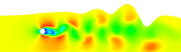
Figure 6: Velocity magnitude in $\Omega_{\ell}$ at time $t=60$.

6 Conclusions

We have presented a compatible, interface-tracking, exactly mass conserving, space-time HDG/EDG discretization for the two-fluid Navier–Stokes equations. The mesh moves with the zero-level set so that the density and viscosity are always piece-wise constants with discontinuity across the interface. Moreover, by using a space-time EDG method for the level-set equation, we are able to obtain a continuous approximation to the interface between the fluids; no smoothing techniques are necessary to accommodate the mesh movement.

Our numerical simulations suggest that the method is energy-stable under mesh movement, and that we can obtain optimal rates of convergence considering that our mesh consists of straight elements. Future work includes extending our discretization to using curved elements near the interface to improve the accuracy of the method and to extend our approach to more general two-fluid flow problems such as rising bubbles in a column and fluid-structure interaction problems.

Acknowledgements

SR gratefully acknowledges support from the Natural Sciences and Engineering Research Council of Canada through the Discovery Grant program (RGPIN-05606-2015).

References

- Kirby et al. [2012] R. M. Kirby, S. J. Sherwin, B. Cockburn, To CG or to HDG: A comparative study, J. Sci. Comput. 51 (2012) 183–212. doi:10.1007/s10915-011-9501-7.
- Yakovlev et al. [2016] S. Yakovlev, D. Moxey, R. M. Kirby, S. J. Sherwin, To CG or to HDG: A comparative study in 3D, J. Sci. Comput. 67 (2016) 192–220. doi:10.1007/s10915-015-0076-6.
- Cockburn et al. [2009] B. Cockburn, J. Gopalakrishnan, R. Lazarov, Unified hybridization of discontinuous Galerkin, mixed, and continuous Galerkin methods for second order elliptic problems, SIAM J. Numer. Anal. 47 (2009) 1319–1365. doi:10.1137/070706616.
- Fu [2019] G. Fu, An explicit divergence-free DG method for incompressible flow, Comput. Methods Appl. Mech. Engrg. 345 (2019) 502–517. doi:10.1016/j.cma.2018.11.012.
- Lehrenfeld and Schöberl [2016] C. Lehrenfeld, J. Schöberl, High order exactly divergence-free hybrid discontinuous galerkin methods for unsteady incompressible flows, Comput. Methods Appl. Mech. Engrg. 307 (2016) 339–361. doi:10.1016/j.cma.2016.04.025.
- Rhebergen and Wells [2018] S. Rhebergen, G. N. Wells, A hybridizable discontinuous Galerkin method for the Navier–Stokes equations with pointwise divergence-free velocity field, J. Sci. Comput. 76 (2018) 1484–1501. doi:10.1007/s10915-018-0671-4.
- Cockburn et al. [2009] B. Cockburn, J. Guzmán, S.-C. Soon, H. K. Stolarski, An analysis of the embedded discontinuous Galerkin method for second-order elliptic problems, SIAM J. Numer. Anal. 47 (2009) 2686–2707. doi:10.1137/080726914.
- Güzey et al. [2007] S. Güzey, B. Cockburn, H. Stolarski, The embedded discontinuous Galerkin methods: Application to linear shells problems, Internat. J. Numer. Methods Engrg. 70 (2007) 757–790. doi:10.1002/nme.1893.
- Rhebergen and Wells [2020] S. Rhebergen, G. N. Wells, An embedded-hybridized discontinuous Galerkin finite element method for the Stokes equations, Comput. Methods Appl. Mech. Engrg. 367 (2020). doi:10.1016/j.cam.2019.112476.
- Osher and Sethian [1988] S. Osher, J. A. Sethian, Fronts propagating with curvature-dependent speed: Algorithms based on Hamilton–Jacobi formulations, J. Comput. Phys. 79 (1988) 12–49. doi:10.1016/0021-9991(88)90002-2.
- Chang et al. [1996] Y. C. Chang, T. Y. Hou, B. Merriman, S. Osher, A level set formulation of Eulerian interface capturing methods for incompressible fluid flows, J. Comput. Phys. 124 (1996) 449–464. doi:10.1006/jcph.1996.0072.
- Sussman et al. [1994] M. Sussman, P. Smereka, S. Osher, A level set approach for computing solutions to incompressible two-phase flow, J. Comput. Phys. 114 (1994) 146–159. doi:10.1006/jcph.1994.1155.
- Grooss and Hesthaven [2006] J. Grooss, J. Hesthaven, A level set discontinuous galerkin method for free surface flows, Comput. Methods Appl. Mech. Engrg. 195 (2006) 3406–3429. doi:j.cma.2005.06.020.
- Lin et al. [2005] C. Lin, H. Lee, T. Lee, L. J. Weber, A level set characteristic Galerkin finite element method for free surface flows, Int. J. Numer. Meth. Fluids 49 (2005) 521–547. doi:10.1002/fld.1006.
- Marchandise and Remacle [2006] E. Marchandise, J.-F. Remacle, A stabilized finite element method using a discontinuous level set approach for solving two phase incompressible flows, J. Comput. Phys. 219 (2006) 780–800. doi:10.1016/j.jcp.2006.04.015.
- Labeur and Wells [2009] R. J. Labeur, G. N. Wells, Interface stabilised finite element method for moving domains and free surface flows, Comput. Methods Appl. Mech. Engrg. 198 (2009) 615–630. doi:10.1016/j.cma.2008.09.014.
- Fu [2020] G. Fu, Arbitrary Lagrangian–Eulerian hybridizable discontinuous Galerkin methods for incompressible flow with moving boundaries and interfaces, Comput. Meth. Appl. Mech. Engrg. 367 (2020). doi:10.1016/j.cma.2020.113158.
- Neunteufel and Schöberl [2020] M. Neunteufel, J. Schöberl, Fluid-structure interaction with h(div)-conforming finite elements, arXiv preprint arXiv:2005.06360 (2020).
- van der Vegt and Sudirham [2008] J. J. W. van der Vegt, J. J. Sudirham, A space-time discontinuous Galerkin method for the time-dependent Oseen equations, Appl. Numer. Math. 58 (2008) 1892–1917. doi:10.1016/j.apnum.2007.11.010.
- Hughes and Hulbert [1988] T. J. R. Hughes, G. M. Hulbert, Space-time finite element methods for elastodynamics: Formulations and error estimates, Comput. Methods Appl. Mech. Engrg. 66 (1988) 339–363. doi:10.1016/0045-7825(88)90006-0.
- Masud and Hughes [1997] A. Masud, T. Hughes, A space-time Galerkin/least-squares finite element formulation of the Navier–Stokes equations for moving domain problems, Comput. Methods Appl. Mech. Engrg. 146 (1997) 91–126. doi:10.1016/S0045-7825(96)01222-4.
- N’dri et al. [2001] D. N’dri, A. Garon, A. Fortin, A new stable space–time formulation for two-dimensional and three-dimensional incompressible viscous flow, Int. J. Numer. Meth. Fluids 37 (2001) 865–884. doi:10.1002/fld.174.
- Zanotti et al. [2015] O. Zanotti, F. Fambri, M. Dumbser, A. Hidalgo, Space–time adaptive ADER discontinuous Galerkin finite element schemes with a posteriori sub-cell finite volume limiting, Computers & Fluids 118 (2015) 204–224. doi:10.1016/j.compfluid.2015.06.020.
- Horvath and Rhebergen [2019] T. L. Horvath, S. Rhebergen, A locally conservative and energy-stable finite element method for the Navier–Stokes problem on time-dependent domains, Int. J. Numer. Meth. Fluids 89 (2019) 519–532. doi:10.1002/fld.4707.
- Horvath and Rhebergen [2020] T. L. Horvath, S. Rhebergen, An exactly mass conserving space-time embedded-hybridized discontinuous galerkin method for the Navier–Stokes equations on moving domains, J. Comput. Phys. 417 (2020). doi:10.1016/j.jcp.2020.109577.
- Aizinger and Dawson [2006] V. Aizinger, C. Dawson, The local discontinuous Galerkin method for three-dimensional shallow water flow, Comput. Methods Appl. Mech. Engrg. 196 (2006) 734–746. doi:10.1016/j.cma.2006.04.010.
- Dawson et al. [2004] C. Dawson, S. Sun, M. F. Wheeler, Compatible algorithms for coupled flow and transport, Comput. Methods Appl. Mech. Engrg. 193 (2004) 2565–2580. doi:10.1016/j.cma.2003.12.059.
- van der Vegt and van der Ven [2002] J. J. W. van der Vegt, H. van der Ven, Space-time discontinuous Galerkin finite element method with dynamic grid motion for inviscid compressible flows. i. General formulation, J. Comput. Phys. 182 (2002) 546–585. doi:10.1006/jcph.2002.7185.
- Wells [2011] G. N. Wells, Analysis of an interface stabilized finite element method: the advection-diffusion-reaction equation, SIAM J. Numer. Anal. 49 (2011) 87–109. doi:10.1137/090775464.
- Cesmelioglu and Rhebergen [2021] A. Cesmelioglu, S. Rhebergen, A compatible embedded-hybridized discontinuous Galerkin method for the Stokes–Darcy-transport problem, Commun. Appl. Math. Comput. (2021). doi:10.1007/s42967-020-00115-0.
- Gagarina et al. [2014] E. Gagarina, V. R. Ambati, J. J. W. van der Vegt, O. Bokhove, Variational space-time (dis)continuous Galerkin method for nonlinear free surface water waves, J. Comput. Phys. 275 (2014) 459–483. doi:10.1016/j.jcp.2014.06.035.
- van der Vegt and Xu [2007] J. J. W. van der Vegt, Y. Xu, Space-time discontinuous Galerkin method for nonlinear water waves, J. Comput. Phys. 224 (2007) 17–39. doi:10.1016/j.jcp.2006.11.031.
- Dobrev et al. [2020] V. A. Dobrev, T. V. Kolev, et al., MFEM: Modular finite element methods, http://mfem.org, 2020.
- Rivière [2008] B. Rivière, Discontinuous Galerkin Methods for Solving Elliptic and Parabolic Equations, volume 35 of Frontiers in Applied Mathematics, Society for Industrial and Applied Mathematics, Philadelphia, 2008.
- Kirk and Rhebergen [2019] K. Kirk, S. Rhebergen, Analysis of a pressure-robust hybridized discontinuous Galerkin method for the stationary Navier–Stokes equations, J. Sci. Comput. 81 (2019) 881–897. doi:10.1007/s10915-019-01040-y.
- Huynh et al. [2013] L. N. T. Huynh, N. C. Nguyen, J. Peraire, B. C. Khoo, A high-order hybridizable discontinuous Galerkin method for elliptic interface problems, Int. J. Numer. Meth. Engng. 93 (2013) 183–200. doi:10.1002/nme.4382.
- Wang and Khoo [2013] B. Wang, B. C. Khoo, Hybridizable discontinuous Galerkin method (HDG) for Stokes interface flow, J. Comput. Phys. 247 (2013) 262–278. doi:10.1016/j.jcp.2013.03.064.
- Wu et al. [2001] G. X. Wu, R. E. Taylor, D. M. Greaves, The effect of viscosity on the transient free-surface waves in a two-dimensional tank, J. Eng. Math. 40 (2001) 77–90. doi:10.1023/A:1017558826258.
- Schäfer et al. [1996] M. Schäfer, S. Turek, F. Durst, E. Krause, R. Rannacher, Benchmark computations of laminar flow around a cylinder, in: E. H. Hirschel (Ed.), Flow Simulation with High-Performance Computers II, 1996, pp. 547–566.