Cosmography with Standard Sirens from the Einstein Telescope

Abstract

We discuss the power of third-generation gravitational wave detectors to constrain cosmographic parameters in the case of electromagnetically bright standard sirens focusing on the specific case of the Einstein Telescope. We analyze the impact that the redshift source distribution, the number of detections and the observational error in the luminosity distance have on the inference of the first cosmographic parameters, and show that with a few hundreds detections the Hubble constant can be recovered at sub-percent level whereas the deceleration parameter at a few percent level, both with negligible bias.

I Introduction

The rising of Gravitational Wave (GW) Astronomy has opened new ways to investigate phenomena not only in astronomy, but also in fundamental physics and cosmology. The large interferometric second generation detectors LIGO TheLIGOScientific:2014jea and Virgo TheVirgo:2014hva are presently in their advanced phase, and they will be joined in the next observation run by KAGRA KAGRA:2020tym , having already confirmed 90 detections LIGOScientific:2018mvr ; LIGOScientific:2020ibl ; LIGOScientific:2021djp . In the next decade third-generation GW detectors, like Einstein Telescope punturo2010third and Cosmic Explorer Reitze:2019iox , will join the scientific quest for GWs and detections of coalescing binaries will become a routine in astronomy, being already at the level of $\sim\,O(1)$ per week with second-generation detectors.

For cosmological applications, GWs from coalescing binaries are an invaluable tool as they are standard sirens Schutz:1986gp (see also Holz:2005df ; Dalal:2006qt ; Nissanke:2009kt ): the intrinsic property of a binary system, like masses and spins, can be inferred from a detailed analysis of the characteristic chirp shape of the signal, leading to an unbiased estimation of the luminosity distance, modulo a degeneracy with some geometric orientation angles, which can in principle be disentangled by observation via multiple detectors, see e.g. Vitale:2016icu for explicit simulations. It follows that an outstanding cosmological application of GW detections from coalescing binaries is to measure the distance versus redshift relation, if the redshift of the source is available. On general grounds GW detections cannot measure the redshift of the source, but redshift can be estimated by adding extra information, like host galaxy identification via electromagnetic counterpart, as it happened for the GW170817 detected jointly with the short GRB 170817A and the optical transient AT 2017gfo LIGOScientific:2017ync , or using galaxy catalogs either via statistical identification of host galaxies Schutz:1986gp ; DelPozzo:2011vcw ; DES:2019ccw , or by a full cross-correlation of GW sky localization with spatial correlation functions Oguri:2016dgk ; Mukherjee:2020hyn ; Diaz:2021pem , see also Canas-Herrera:2019npr ; Canas-Herrera:2021qxs ; Zhang:2019loq ; Jin:2020hmc ; Jin:2021pcv .

Other possibilities to fold in redshift information have been investigated using e.g. tidal effects which can break the gravitational mass-redshift degeneracy Messenger:2011gi , the astrophysical mass-gap Heger:2002by in solar mass black holes, as done in Farr:2019twy ; Ezquiaga:2020tns ; You:2020wju ; Mastrogiovanni:2021wsd , or the prior knowledge of source redshift distributions Ding:2018zrk ; Leandro:2021qlc .

In this work we focus on the case in which the host galaxy is identified via an electromagnetic counterpart, so that redshift can be measured with negligible error, while the luminosity distance is measured gravitationally, aiming at determining the luminosity distance versus redshift relation in a model-independent way, i.e. without relying in a specific background cosmological model, adopting the cosmography approach Weinberg:1972kfs . We thus investigate how well the time derivatives of the cosmological scale factor can be determined using the information that electromagnetically bright GW standard sirens will reveal with third-generation detectors, expected to be operating in the next decade.

The paper is organized as follows: in Sec. II we briefly review the cosmographic expansion whereas the simulated data used in the statistical analysis are detailed in Sec. III. The main results of the paper are presented and discussed in Sec. IV. Sec. V presents the conclusions that can be drawn from our analysis.

II The cosmographic expansion

Let us consider the flat Friedmann-Lemaître-Robertson-Walker metric ($c=1$)

$$ds^{2}=-dt^{2}+a^{2}(t)\left[dr^{2}+r^{2}(d\theta^{2}+\sin^{2}\theta d\phi^{2})\right]\,,$$ (1)

where $a(t)$ is the scale factor. One can Taylor-expand its time dependence

$$a(t)=a_{0}\left\{1+H_{0}(t-t_{0})-\frac{1}{2}q_{0}[H_{0}(t-t_{0})]^{2}+\frac{1}{6}j_{0}[H_{0}(t-t_{0})]^{3}\right.$$

$$\left.+\frac{1}{24}s_{0}[H_{0}(t-t_{0})]^{4}+\frac{1}{120}l_{0}[H_{0}(t-t_{0})]^{5}+O(6)\right\}\,,$$ (2)

where $H_{0}$ is the Hubble constant, $a_{0}\equiv a(t_{0})$ being $t_{0}$ the present time, and the remaining constants appearing in the expansion have been conveniently expressed as

$$\begin{array}[]{rclrcl}\displaystyle q_{0}&=&\displaystyle-\frac{1}{H_{0}^{2}}\left(\frac{1}{a}\frac{d^{2}a}{dt^{2}}\right)\bigg{|}_{t=t_{0}}\,,&\displaystyle\quad j_{0}&=&\displaystyle\frac{1}{H_{0}^{3}}\left(\frac{1}{a}\frac{d^{3}a}{dt^{3}}\right)\bigg{|}_{t=t_{0}},\\ \displaystyle s_{0}&=&\displaystyle\frac{1}{H_{0}^{4}}\left(\frac{1}{a}\frac{d^{4}a}{dt^{4}}\right)\bigg{|}_{t=t_{0}}\,,&\displaystyle\quad l_{0}&=&\displaystyle\frac{1}{H_{0}^{5}}\left(\frac{1}{a}\frac{d^{5}a}{dt^{5}}\right)\bigg{|}_{t=t_{0}}\,,\end{array}$$ (3)

where $H\equiv a^{-1}da/dt$. The parameters $q_{0},j_{0},s_{0},l_{0}$ are called respectively deceleration, jerk, snap and lerk parameters visser2004jerk ; Cattoen:2007sk ; aviles2012cosmography ; Lazkoz:2013ija . From these equations we can also obtain zhang2017we

$$H(z)=H_{0}\left\{1+(1+q_{0})z+\frac{1}{2}(j_{0}-q_{0}^{2})z^{2}+\frac{1}{6}[3q_{0}^{2}+3q_{0}^{3}-4q_{0}j_{0}-3j_{0}-s_{0}]z^{3}+\right.$$

$$+\left.\frac{1}{24}(-12q_{0}^{2}-24q_{0}^{3}-15q_{0}^{4}+32q_{0}j_{0}+25q_{0}^{2}j_{0}+7q_{0}s_{0}+12j_{0}-4j_{0}^{2}+8s_{0}+l_{0})z^{4}+O(z^{5})\right\}\;,$$ (4)

where $1+z\equiv 1/a(t)$. To make contact with observations it is useful to define the luminosity distance expression

$$d_{L}(z)=\left(1+z\right)\int_{0}^{z}\frac{dz^{\prime}}{H(z^{\prime})}\,,$$ (5)

which, in terms of the cosmographic parameters Eq. (II), can be expressed as

$$d_{L}(z) = \frac{1}{H_{0}}\Bigl{[}z+z^{2}\Bigl{(}\frac{1}{2}-\frac{q_{0}}{2}\Bigr{)}+z^{3}\Bigl{(}-\frac{1}{6}-\frac{j_{0}}{6}+\frac{q_{0}}{6}+\frac{q_{0}^{2}}{2}\Bigr{)}$$ (6)

$$+z^{4}\Bigl{(}\frac{1}{12}+\frac{5j_{0}}{24}-\frac{q_{0}}{12}+\frac{5j_{0}q_{0}}{12}-\frac{5q_{0}^{2}}{8}-\frac{5q_{0}^{3}}{8}+\frac{s_{0}}{24}\Bigr{)}+$$

$$+z^{5}\Bigl{(}-\frac{1}{20}-\frac{9j_{0}}{40}+\frac{j_{0}^{2}}{12}-\frac{l_{0}}{120}+\frac{q_{0}}{20}-\frac{11j_{0}q_{0}}{12}+\frac{27q_{0}^{2}}{40}-\frac{7j_{0}q_{0}^{2}}{8}+\frac{11q_{0}^{3}}{8}+\frac{7q_{0}^{4}}{8}-\frac{11s_{0}}{120}-\frac{q_{0}s_{0}}{8}\Bigr{)}$$

$$+z^{6}\Bigl{(}\frac{1}{30}+\frac{7j_{0}}{30}-\frac{19j_{0}^{2}}{72}+\frac{19l_{0}}{720}+\frac{m_{0}}{720}-\frac{q_{0}}{30}+\frac{13j_{0}q_{0}}{9}-\frac{7j_{0}^{2}q_{0}}{18}+\frac{7l_{0}q_{0}}{240}-\frac{7q_{0}^{2}}{10}+\frac{133j_{0}q_{0}^{2}}{48}$$

$$-\frac{13q_{0}^{3}}{6}+\frac{7j_{0}q_{0}^{3}}{4}-\frac{133q_{0}^{4}}{48}-\frac{21q_{0}^{5}}{16}+\frac{13s_{0}}{90}-\frac{7j_{0}s_{0}}{144}+\frac{19q_{0}s_{0}}{48}+\frac{7q_{0}^{2}s_{0}}{24}\Bigr{)}+O(z^{7})\Bigr{]}.$$

Observation of a set of $\{d_{Li}\}$ and corresponding $\{z_{i}\}$ data points will enable the determination of the cosmographic parameters, whose accuracy will depend on the quality and range of available data, as we will discuss in the next Section. Note that any finite order truncation of the series (6) is badly behaved for $z>1$. However, as it will be shown, for the range of redshift of interest for the present work, we can safely work with (a truncation of) Eq. (6).

III Simulated data

To test the accuracy of the cosmographic expansion applied to GW standard sirens, we set the fiducial model to be the flat $\Lambda$CDM cosmology, with the matter density parameter $\Omega_{M}=0.311$ and $H_{0}=67.66$ km/sec/Mpc, in agreement with the current Cosmic Microwave Background analysis of Planck:2018vyg . Note that the present controversy on the value of $H_{0}$ – with low-redshift determinations in contrast with early-Universe ones by more than 4$\sigma$ level 2018ApJ…855..136R ; Birrer:2018vtm ; Verde:2019ivm ; refId0 – does not affect our analysis, which aims at quantifying the uncertainties on the cosmographic parameters expected from upcoming joint GW and electromagnetic data.

The cosmographic parameters (up to sixth order) for the $\Lambda$CDM model are written as:

$$\begin{array}[]{rcl}\displaystyle q_{0}&=&\displaystyle\frac{3}{2}\Omega_{M}-1\,,\\ \displaystyle j_{0}&=&\displaystyle 1\,,\\ \displaystyle s_{0}&=&\displaystyle 1-\frac{9}{2}\Omega_{M}\,,\\ \displaystyle l_{0}&=&\displaystyle 1+3\Omega_{M}-\frac{27}{2}\Omega_{M}^{2}\,,\\ \displaystyle m_{0}&=&\displaystyle 1-\frac{27}{2}\Omega_{M}^{2}-81\Omega_{M}^{2}-\frac{81}{2}\Omega_{M}^{3}\,,\end{array}$$ (7)

whose numerical values for our fiducial model are summarized in Tab. 1.

$q_{0}$	$j_{0}$	$s_{0}$	$l_{0}$	$m_{0}$
$\quad-0.533\quad$	$\quad 1\quad$	$\quad-0.4\quad$	$\quad 0.627\quad$	$\quad-9.365\quad$

Table 1: Cosmographic parameters in a flat $\Lambda$CDM cosmology with $\Omega_{M}=0.311$.

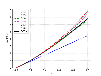
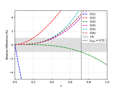
Figure 1: Left) Luminosity distance $d_{L}$ for different orders of the cosmographic series – Eq. (6). The black curve represents the fiducial $\Lambda$CDM model adopted in the analysis. Right) Relative difference between the cosmographic series and the fiducial cosmology. The shadowed horizontal region stands for a difference of 1%, which is reached at $z_{cut}=0.72$ (vertical dotted line) by the third order series.

As mentioned earlier, the $d_{L}$ expansion in $z$ converges for $z<1$ Cattoen:2007sk . However, to have a faithful reconstruction of the underlying model with only a handful of terms one needs to restrict the redshift to lower values. In Fig. 1 (left panel) we show the behavior of $d_{L}$ as a function of the redshift for different orders of the cosmographic series given in Eq.(6), with values of the cosmographic parameters reported in Tab. 1. For comparison, our fiducial model is also shown (black curve). The right panel shows the relative difference between the cosmographic series and the fiducial cosmology. As it can be seen, the series truncated at third order deviates less than $1\%$ from the fiducial model in the redshift interval $0<z<0.72$, which in turn defines the redshift interval adopted in this work to assess the precision with which one can recover the first three cosmographic parameters. Note that the cosmographic parameter values reported in Tab. 1 are the ones which reproduce exactly the Taylor expansion of the $\Lambda$CDM model with $\Omega_{M}=0.311$, hence it is expected that truncating the $z$-expansion at any finite order, the best fit values of the cosmographic parameters will be different from these ones.

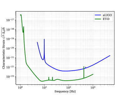
Figure 2: Left) Dimensionless strain sensitivity for Advanced LIGO, from “Zero Detuning High Power” spectral noise density implemented in LALSuite lalsuite , and Einstein Telescope, adopting the noise spectral density “D” from Hall:2019xmm . Right) Sensitivity region, defined as the distance at which the $SNR$ of Eq. (8) is larger than the conventional threshdold value $8$, for spin-less equal mass systems with optimal orientation with respect to the detector (only the GW dominant mode has been used). The dashed area highlights total mass values for which an electromagnetic counterpart is expected.

III.1 Source Distributions

For the simulation of third generation detector observations we focus on the Einstein Telescope punturo2010third , whose noise spectral density is report in Fig. (2) together with the advanced LIGO one.

The signal-to-noise ratio $SNR$ of a real-time GW signal $h(t)$ is defined in terms of its Fourier-transform $\tilde{h}(f)$ via

$$SNR^{2}\equiv 4\int_{0}^{\infty}\frac{|\tilde{h}(f)|^{2}}{S_{n}(f)}\,df\,,$$ (8)

where the noise spectral density $S_{n}(f)$ is defined in terms of the detector noise $\tilde{n}(f)$ averaged over many realizations

$$\langle\tilde{n}(f)\tilde{n}^{*}(f^{\prime})\rangle=S_{n}(f)\delta(f-f^{\prime})\,.$$ (9)

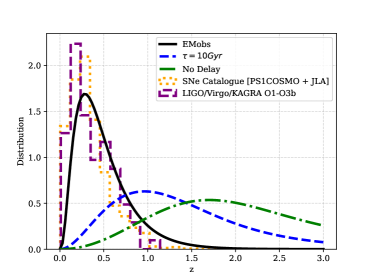
Figure 3: Left) Expected normalized distributions of EM bright GW events detected in coincidence by the Einstein Telescope and future EM observatory Theseus Eq. (13) Belgacem:2019tbw or dictated by (delayed) star formation rate (Eq. 12). For comparison, the normalized distributions of presently confirmed events by the LIGO/Virgo/KAGRA collaboration and of the SuperNovae catalog events betoule2014improved ; 2018ApJ…859..101S ; 2018ApJ…857…51J are also reported. Right) Error budget of luminosity distance gravitational measure – see Eqs. (14) and (15).

The redshift distribution of coalescing events is largely unknown, hence to make an analysis as comprehensive as possible we follow deSouza:2019ype and produce and analyze mock data corresponding to three astrophysical source distributions to check how they affect the parameter estimation. We thus consider:

1. Detected merger distribution per comoving volume following the star formation rate given in madau2014cosmic :

   $$\psi(z)\propto\frac{\left(1+z\right)^{2.7}}{1+\left(\frac{1+z}{2.9}\right)^{5.6}}\,,$$ (10)

2. Merger distribution obtained with a stochastic delay with respect to the star formation rate, the delay being Poisson-distributed with average $\tau=10$ Gyr, as shown in (vitale2017parameter, ), with a merger rate per unit comoving volume ${\cal R}_{m}$ given by (modulo normalization)

   $${\cal R}_{m}(z_{m},\tau)\propto\int_{z_{m}}^{\infty}dz_{f}\frac{dt}{dz_{f}}\psi(z_{f})\exp\left[-\frac{t(z_{f})-t(z_{m})}{\tau}\right]\,.$$ (11)

   Note that in both this and the previous case, the detected merger rate $R_{m}$ is related to the density merger rate of (11) via

   $$\begin{array}[]{rcl}\displaystyle R_{m}(z,\tau)&\equiv&\displaystyle\frac{d^{2}N_{m}}{dt_{o}dz}=\frac{1}{1+z}\frac{dV_{c}}{dz}{\cal R}_{m}(z,\tau)\\ &=&\displaystyle\frac{4\pi d_{L}^{2}(z)}{(1+z)^{3}H(z)}{\cal R}_{m}(z,\tau)\,.\end{array}$$ (12)

3. A distribution considering that only close enough events will have a detectable EM counterpart. With a dedicated EM detector like THESEUS amati2018theseus ; Belgacem:2019tbw it can be represented as shown in Fig. (3) (“EMobs” line) deSouza:2019ype

   $$R_{EMobs}\propto\frac{z^{3}}{1+\exp(10.6\,z^{0.6})}\,.$$ (13)

III.2 Luminosity distance uncertainty

Having fixed the source redshift distribution, we now discuss the uncertainties in the luminosity distance measurements by the third generation gravitational wave detector Einstein Telescope. The main contributions are given by zhao2011determination ; Gordon:2007zw :

$$\frac{\Delta d_{L}(z)}{d_{L}(z)}=\displaystyle\left[\left(\frac{\Delta d_{L}(z)}{d_{L}(z)}\right)_{ET}^{2}+\left(\frac{\Delta d_{L}(z)}{d_{L}(z)}\right)_{Lensing}^{2}+\left(\frac{\Delta d_{L}(z)}{d_{L}(z)}\right)_{v_{pec}}^{2}\right]^{1/2}\,,$$ (14)

with

$$\begin{array}[]{lcl}\displaystyle\left(\frac{\Delta d_{L}(z)}{d_{L}(z)}\right)_{ET}&\approx&\displaystyle 0.1449z-0.0118z^{2}+0.0012z^{3}\quad,\\ \displaystyle\left(\frac{\Delta d_{L}(z)}{d_{L}(z)}\right)_{Lensing}&\approx&\displaystyle 0.066\left[4\left(1-(1+z)^{-1/4}\right)\right]^{1.8}\quad,\\ \displaystyle\left(\frac{\Delta d_{L}(z)}{d_{L}(z)}\right)_{v_{pec}}&\approx&\displaystyle\bigg{|}1-\frac{(1+z)^{2}}{H(z)d_{L}(z)}\bigg{|}\frac{\sigma_{v}}{c},\quad\sigma_{v}=331\ {\rm{km/s}}\,,\end{array}$$ (15)

where the error budget has been divided respectively into instrumental, lensing and peculiar velocity contributions. As the systematic errors due peculiar velocities of galaxies are important only for $z\lesssim 0.1$, they do not play an important role in this work. In Fig. (4), we show the simulated data of $d_{L}(z)$ using the EMobs distribution given by Eq. (13). The red curve represents the fiducial model used in the simulation whereas the light blue and dark blue regions stand respectively for 1- and 2-$\sigma$ error band, being $\sigma$ the quantity $\Delta d_{L}$, given the error budget (Eq. 14).

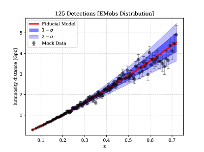
Figure 4: Mock data using the EMobs distribution Eq. (13). The fiducial $\Lambda$CDM model is denoted by the red line, blue bands denote 1- and 2-$\sigma$ confidence regions.

III.3 Parameter Estimation

We adopt a Bayesian framework to estimate the parameters $\{\theta_{i}\}=\{H_{0},q_{0},j_{0}\}$ given the model $\cal M$ represented by the cosmographic expansion (6) truncated at third order. In this context the combined probability distribution functions of parameters $\theta_{i}$ are given by

$$P(\{\theta_{i}\}|d,\ \mathcal{M})=\frac{P(d|\{\theta_{i}\},\ \mathcal{M})P(\{\theta_{i}\}|,\ \mathcal{M})}{P(d)}\,,$$ (16)

where the likelihood $P(d|\{\theta_{i}\},\ \mathcal{M})$ is given by:

$$P(d|\{\theta_{i}\},\ \mathcal{M})=\exp\left[-\frac{1}{2}\sum_{i=1}^{N}\frac{|d_{i}-f_{i}(\{\theta_{i}\},z_{i})|}{\sigma_{i}^{2}}\right]\,,$$ (17)

being $N$ the number of detections, $d_{i}$ the data with error $\sigma_{i}$ and $f_{i}(\{\theta_{i}\},z_{i})$ is the parameter-dependent model function (third order truncation of Eq. 6) and the priors on $H_{0}$, $q_{0}$, and $j_{0}$ are taken to be flat in the region respectively $[54,81]$km/sec/Mpc, $[-1,0]$, $[-1,3]$. Note that we have neglected the error on the redshift, consistently with the assumption of an EM counterpart for the GW signal, that allows determination of the host galaxy determination. To perform our analysis we use the Bilby software Ashton:2018jfp with the Nestle sampler, Mukherjee:2005wg which implements the nestled sampling algorithm Skilling:2006gxv , with 500 live points.

In the next section we estimate the errors and the biases in the cosmographic parameters $H_{0}$, $q_{0}$ and $j_{0}$ for the three source distributions introduced in Subsec. III.1, and discuss how such estimates change as data at different redshift ranges are considered.

IV Results

As mentioned earlier, we restrict the redshift range to $0<z<0.72$, which corresponds to the region where the third order cosmographic expansion can faithfully reproduce the underlying cosmological model up to one percent level. Incidentally, this is the redshift range for which the large majority of detection will be made if sources follow the realistic distribution (13). Besides the parameter uncertainty $\sigma_{\theta_{i}}$, defined by the 68% confidence interval of its probability distribution function, we also report the relative bias, defined as the absolute value of the difference between the average value recovered and injected one normalized by $\sigma_{\theta_{i}}$.

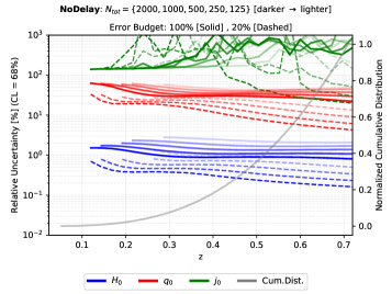
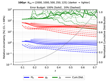
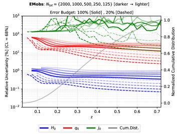
Figure 5: Results for parameter estimation error for (top) the source distribution following star formation rate (10), (middle) $10$ Gyr average delay between star formation and binary merger, and (bottom) EMobs (13) as a function of the highest redshift detection. Lines get thicker as the number of total detections increases. Solid lines are for luminosity distance error as in Eq. (14), dot-dashed for 20% of such value. The right vertical scale refers to the normalized cumulative distribution of detections, displayed in light grey.

In Fig. (5) we report the measurement of the uncertainty for the three cosmographic parameters. For each of them we show how such error varies with the redshift range of the detections, for five fixed values of total number of detections, ranging from 125 up to 2,000. The total number of detections refer to the complete redshift range up to $z=0.72$, hence the process of accumulating detections in a realistic case will move the parameter uncertainty from lighter lines (smaller numbers of total detections) to darker lines (larger numbers). For completeness, we also consider two possible values of the luminosity distance uncertainties in the measure, the value given in Eq. (14) and 20% of that, which saturates the lensing contribution in (15). For each set of simulations, the result is obtained by averaging over $500$ random realizations of injections extracted from the relevant redshift distribution. Similarly, in Fig. (6) we show the bias for the three cosmographic parameters, computed as the absolute value of the difference between the mean value and the injected value, normalized by $\sigma_{\theta_{i}}$. For each of them we report how they vary with redshift range for the same five fixed values of total number of detections.

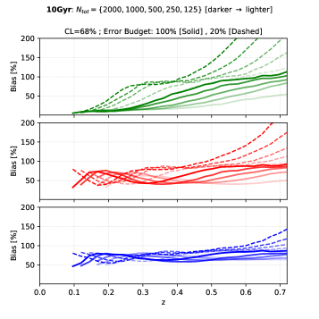
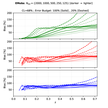
Figure 6: The same as in Fig. (5) for the parameter biases.

We note from Fig. 6 that the best fit values of the cosmographic parameters deviates from the values of Tab. 1 when detections at redshift $z\gtrsim 0.4$ are included. To better illustrate this aspect, we report the distributions of the best fit values of the cosmographic parameters $H_{0}$, $q_{0}$, and $j_{0}$ for the different source distributions discussed in Subsec. III.1 obtained over 500 realizations, for detections up to redshift $z_{c}=0.71$ in Fig. 7, and up redshift $0.4$ in Fig. 8. Clearly detections at higher redshift tend to shift the best fit to values incompatible to those obtained via the exact cosmographic expansion of $\Lambda$CDM given in Tab.1, the effect being stronger for astrophysical distributions having more events at high redshift. However the bias effect is visible only when the measure error of the luminosity distance is reduced to the lensing contribution, i.e. to 20% its realistic value.

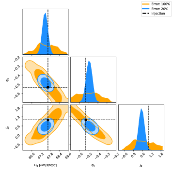
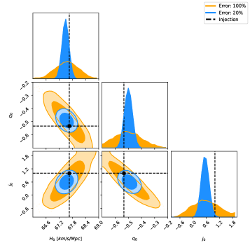
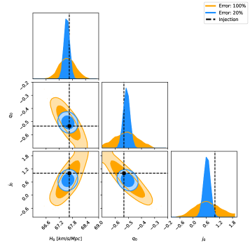
Figure 7: Marginalized posterior distributions of the cosmographic parameter mean values for 500 realizations of 1,000 events drawn from No-Delay distributions (top left), $\tau=10Gyr$ delay (top right) and EMobs (bottom), see Subsec. III.1. For each distribution the case for 100% and 20% the error given in Eq. (15) are reported.

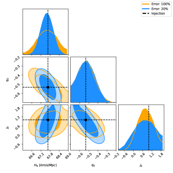
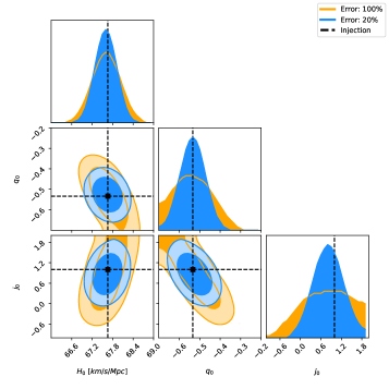
Figure 8: Same as Fig. (7) for detections up to $z=0.4$, corresponding to $\sim$ 180, 261, 586 for no-delay, 10 Gyr and EMobs distributions respectively.

Finally, we also find useful to compare the results obtained from GW detections with the current estimates of the first three cosmographic parameters from type Ia supernovae (SNe) data 2018ApJ…857…51J . We adopt the same cutoff in redshift, $z_{cut}=0.72$, which results in a SNe subsample with 972 data points, and fix the absolute peak magnitude at $M_{B}=-19.214\pm 0.037$ mag, as given by Riess:2020fzl . Our analysis gives $H_{0}=75.23^{+0.40}_{-0.38}$ km/sec/Mpc, $q_{0}=-0.70\pm 0.10$, $j_{0}=1.78^{+0.78}_{-0.74}$, with the error bars corresponding to 68% confidence limit. As shown in Fig. (9), GWs detections can reach a better precision than current SNe data in measurements of $H_{0}$ for a number of detection larger than about 1,000 considering the standard errors on $d_{L}$, and for $\sim$ 100 detections when the errors are reduced to 20%, the value of Eq. (15), see also Tab. 2 and Tab. 3.

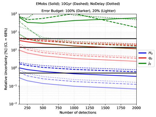
Figure 9: Comparisons between the error estimations for $H_{0}$, $q_{0}$, and $j_{0}$ from standard sirens (for three source distributions and different number of detections) and SNe data 2018ApJ…859..101S (horizontal black lines from bottom to top). In all cases only SNe up to redshift $z_{cut}=0.72$ have been considered, which correspond to 972 detections.

	$|\Delta H_{0}|$ km/s/Mpc		$|\Delta q_{0}|$		$|\Delta j_{0}|$
	500 sirens	1000 sirens	500 sirens	1000 sirens	500 sirens	1000 sirens
EMobs	0.44	0.33	0.11	0.08	0.74	0.55
10Gyr	0.75	0.58	0.15	0.12	0.84	0.66
NoDelay	0.95	0.74	0.17	0.14	0.93	0.74

Table 2: $1$-$\sigma$ parameter uncertainties $\sigma_{\theta_{i}}$ from 500 and 1000 standard sirens detections up to redshift $z=0.72$, for $d_{L}$ measurement uncertainty given by Eq. (14) for sources distributed according to the EMobs, 10Gyr and NoDelay distributions.

	$|\Delta H_{0}|$ (km/s/Mpc)		$|\Delta q_{0}|$		$|\Delta j_{0}|$
	500 sirens	1000 sirens	500 sirens	1000 sirens	500 sirens	1000 sirens
EMobs	0.09	0.07	0.02	0.02	0.16	0.11
10Gyr	0.17	0.12	0.04	0.02	0.20	0.14
NoDelay	0.23	0.16	0.04	0.03	0.23	0.16

Table 3: $1$-$\sigma$ parameter uncertainties $\sigma_{\theta_{i}}$ from 500 and 1000 standard sirens detections up to redshift $z=0.72$ with $d_{L}$ measurement uncertainty reduced to 20%, for sources distributed according to EMobs, 10Gyr and NoDelay distributions.

V Conclusions

We analyzed how future detections of gravitational wave standard sirens by a third generation detector can measure the Hubble constant, the deceleration and the jerk parameters of the cosmographic expansion. As it is well known, truncated cosmographic expansions are not supposed to describe correctly the cosmological expansions beyond redshift of order unity, and we showed that our choice for $z_{cut}=0.72$ leads to a faithful cosmographic model with only the first three cosmographic parameters. The simulated data assumed the contemporary observation of electromagnetic counterparts ensuring redshift determination, and overall detections up to moderate redshift $z_{cut}$.

The results show that the Hubble constant can be measured with sub-percent precision with a few hundred of detections. For higher order parameter in the cosmographic expansion precision is degraded, e.g. for $q_{0}$ one can reach 10% level with 2,000 detections, whereas for $j_{0}$ it is hard to limit precision below 100% level.

Our analysis showed an important caveat, i.e. the best fit values of the third order cosmographic expansion tend to drift away from the exact cosmographic parameter values obtained by a complete Taylor expansion of the underlying $\Lambda$CDM model, when detections at redshit $z\gtrsim 0.4$ are included. While this effect is contained within the 1-$\sigma$ prediction errors for realistic predictions of the luminosity distance measure uncertainty, it is visible when one uses a reduced measurement error on $d_{L}$, corresponding e.g. to the uncertainty induced by lensing of matter structure between source and observer. The reference cosmographic parameters, summarized in Tab. 1, are obtained using the full Taylor expansion of the $d_{L}$ vs. $z$ relation in the $\Lambda$CDM model, hence it is not surprising that the best fit values we obtain for the three cosmographic parameters deviates from them, as also illustrated by Figs.10,11 in Appendix A.

We also analyzed how such results vary with the distribution of events, showing that a distribution more concentrated at low redshifts allows a sharper determination of the $H_{0}$ and $q_{0}$. Besides, the error in the parameter determination is mostly determined by the detections at low redshifts ($\lesssim 0.2$), and then levels off accumulating detections at higher redshifts unless thousands of events are accumulated. We also varied the number of expected detections, whose rate at present is wildly unknown, between realistic values of $O(10^{2})$ and $O(10^{3})$, showing an expected monotonic, sharpening of precision with increasing number of detection. Our projection for the $H_{0}$ measure precision with $\sim$ 1,000 sources is of the same order the one that can be obtained analyzing the presently available SNe data up to $z_{cut}$, as shown in Fig. 9, its exact value varying non-negligibly with the number of detections, their redshift distributions and luminosity distance measurement uncertainty.

Finally, we showed that a crucial ingredient to reduce the measurement error in the cosmographic parameters is represented by the observational uncertainty in $d_{L}$, which can in principle be reduced by correlating observations from separately located detectors, to reach the “lensing limit”, which at moderate redshifts amounts to about 20% of the luminosity distance error budget for a single interferometer.

Appendix A ${\mathbf{\Lambda}}$CDM versus cosmographic expansion

In Figs. 10-11 we show the relative difference between the luminosity distance from the fiducial $\Lambda$CDM model and from the best fit cosmographic one (dashed blue line) and its $1$-$\sigma$ uncertainty. For comparison we also report the differernce between the $\Lambda$CDM model and a cosmographic third order model using the values of $H_{0}$, $q_{0}$ and $j_{0}$ given in Tab. 1. Figs. 10 refer to the three source redshift distributions listed in Subsec. III.1 for realistic luminosity distance uncertainties, and Figs. 10 to the case of reduced $d_{L}$ measurement uncertainty.

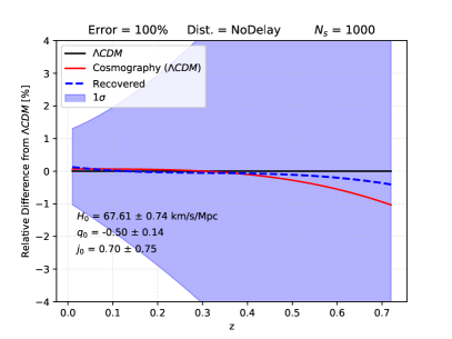
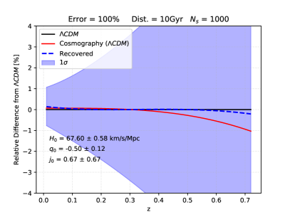
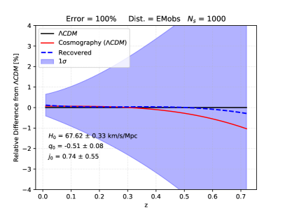
Figure 10: Relative difference between the luminosity distance according to the fiducial model (flat $\Lambda CDM$) and the one recovered from the Bayesian inference with the cosmographic parameters given in Tab. 2 (blue dashed). Also reported is the difference between the fiducial model and the cosmographic one with values of the three cosmographic parameters taken from Tab. 1 (red).

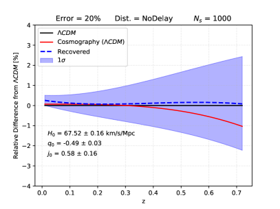
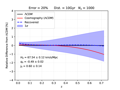
Figure 11: Same as Fig. 10 from simulated data with reduced $d_{L}$ uncertainty measure.

References

- (1) LIGO Scientific collaboration, Advanced LIGO, Class. Quant. Grav. 32 (2015) 074001 [1411.4547].
- (2) VIRGO collaboration, Advanced Virgo: a second-generation interferometric gravitational wave detector, Class. Quant. Grav. 32 (2015) 024001 [1408.3978].
- (3) KAGRA collaboration, Overview of KAGRA: Detector design and construction history, 2005.05574.
- (4) LIGO Scientific, Virgo collaboration, GWTC-1: A Gravitational-Wave Transient Catalog of Compact Binary Mergers Observed by LIGO and Virgo during the First and Second Observing Runs, Phys. Rev. X 9 (2019) 031040 [1811.12907].
- (5) LIGO Scientific, Virgo collaboration, GWTC-2: Compact Binary Coalescences Observed by LIGO and Virgo During the First Half of the Third Observing Run, Phys. Rev. X 11 (2021) 021053 [2010.14527].
- (6) LIGO Scientific, VIRGO, KAGRA collaboration, GWTC-3: Compact Binary Coalescences Observed by LIGO and Virgo During the Second Part of the Third Observing Run, 2111.03606.
- (7) M. Punturo, M. Abernathy, F. Acernese, B. Allen, N. Andersson, K. Arun et al., The third generation of gravitational wave observatories and their science reach, Classical and Quantum Gravity 27 (2010) 084007.
- (8) D. Reitze et al., Cosmic Explorer: The U.S. Contribution to Gravitational-Wave Astronomy beyond LIGO, Bull. Am. Astron. Soc. 51 (2019) 035 [1907.04833].
- (9) B.F. Schutz, Determining the Hubble Constant from Gravitational Wave Observations, Nature 323 (1986) 310.
- (10) D.E. Holz and S.A. Hughes, Using gravitational-wave standard sirens, Astrophys. J. 629 (2005) 15 [astro-ph/0504616].
- (11) N. Dalal, D.E. Holz, S.A. Hughes and B. Jain, Short grb and binary black hole standard sirens as a probe of dark energy, Phys. Rev. D 74 (2006) 063006 [astro-ph/0601275].
- (12) S. Nissanke, D.E. Holz, S.A. Hughes, N. Dalal and J.L. Sievers, Exploring short gamma-ray bursts as gravitational-wave standard sirens, Astrophys. J. 725 (2010) 496 [0904.1017].
- (13) S. Vitale and M. Evans, Parameter estimation for binary black holes with networks of third generation gravitational-wave detectors, Phys. Rev. D95 (2017) 064052 [1610.06917].
- (14) LIGO Scientific, Virgo, Fermi GBM, INTEGRAL, IceCube, AstroSat Cadmium Zinc Telluride Imager Team, IPN, Insight-Hxmt, ANTARES, Swift, AGILE Team, 1M2H Team, Dark Energy Camera GW-EM, DES, DLT40, GRAWITA, Fermi-LAT, ATCA, ASKAP, Las Cumbres Observatory Group, OzGrav, DWF (Deeper Wider Faster Program), AST3, CAASTRO, VINROUGE, MASTER, J-GEM, GROWTH, JAGWAR, CaltechNRAO, TTU-NRAO, NuSTAR, Pan-STARRS, MAXI Team, TZAC Consortium, KU, Nordic Optical Telescope, ePESSTO, GROND, Texas Tech University, SALT Group, TOROS, BOOTES, MWA, CALET, IKI-GW Follow-up, H.E.S.S., LOFAR, LWA, HAWC, Pierre Auger, ALMA, Euro VLBI Team, Pi of Sky, Chandra Team at McGill University, DFN, ATLAS Telescopes, High Time Resolution Universe Survey, RIMAS, RATIR, SKA South Africa/MeerKAT collaboration, Multi-messenger Observations of a Binary Neutron Star Merger, Astrophys. J. Lett. 848 (2017) L12 [1710.05833].
- (15) W. Del Pozzo, Inference of the cosmological parameters from gravitational waves: application to second generation interferometers, Phys. Rev. D 86 (2012) 043011 [1108.1317].
- (16) DES, LIGO Scientific, Virgo collaboration, First Measurement of the Hubble Constant from a Dark Standard Siren using the Dark Energy Survey Galaxies and the LIGO/Virgo Binary–Black-hole Merger GW170814, Astrophys. J. Lett. 876 (2019) L7 [1901.01540].
- (17) M. Oguri, Measuring the distance-redshift relation with the cross-correlation of gravitational wave standard sirens and galaxies, Phys. Rev. D 93 (2016) 083511 [1603.02356].
- (18) S. Mukherjee, B.D. Wandelt, S.M. Nissanke and A. Silvestri, Accurate precision Cosmology with redshift unknown gravitational wave sources, Phys. Rev. D 103 (2021) 043520 [2007.02943].
- (19) C.C. Diaz and S. Mukherjee, Mapping the cosmic expansion history from LIGO-Virgo-KAGRA in synergy with DESI and SPHEREx, 2107.12787.
- (20) G. Cañas Herrera, O. Contigiani and V. Vardanyan, Cross-correlation of the astrophysical gravitational-wave background with galaxy clustering, Phys. Rev. D 102 (2020) 043513 [1910.08353].
- (21) G. Cañas Herrera, O. Contigiani and V. Vardanyan, Learning How to Surf: Reconstructing the Propagation and Origin of Gravitational Waves with Gaussian Processes, Astrophys. J. 918 (2021) 20 [2105.04262].
- (22) J.-F. Zhang, M. Zhang, S.-J. Jin, J.-Z. Qi and X. Zhang, Cosmological parameter estimation with future gravitational wave standard siren observation from the Einstein Telescope, JCAP 09 (2019) 068 [1907.03238].
- (23) S.-J. Jin, D.-Z. He, Y. Xu, J.-F. Zhang and X. Zhang, Forecast for cosmological parameter estimation with gravitational-wave standard siren observation from the Cosmic Explorer, JCAP 03 (2020) 051 [2001.05393].
- (24) S.-J. Jin, L.-F. Wang, P.-J. Wu, J.-F. Zhang and X. Zhang, How can gravitational-wave standard sirens and 21-cm intensity mapping jointly provide a precise late-universe cosmological probe?, Phys. Rev. D 104 (2021) 103507 [2106.01859].
- (25) C. Messenger and J. Read, Measuring a cosmological distance-redshift relationship using only gravitational wave observations of binary neutron star coalescences, Phys. Rev. Lett. 108 (2012) 091101 [1107.5725].
- (26) A. Heger, C.L. Fryer, S.E. Woosley, N. Langer and D.H. Hartmann, How massive single stars end their life, Astrophys. J. 591 (2003) 288 [astro-ph/0212469].
- (27) W.M. Farr, M. Fishbach, J. Ye and D. Holz, A Future Percent-Level Measurement of the Hubble Expansion at Redshift 0.8 With Advanced LIGO, Astrophys. J. Lett. 883 (2019) L42 [1908.09084].
- (28) J.M. Ezquiaga and D.E. Holz, Jumping the Gap: Searching for LIGO’s Biggest Black Holes, Astrophys. J. Lett. 909 (2021) L23 [2006.02211].
- (29) Z.-Q. You, X.-J. Zhu, G. Ashton, E. Thrane and Z.-H. Zhu, Standard-siren cosmology using gravitational waves from binary black holes, Astrophys. J. 908 (2021) 215 [2004.00036].
- (30) S. Mastrogiovanni, K. Leyde, C. Karathanasis, E. Chassande-Mottin, D.A. Steer, J. Gair et al., Cosmology in the dark: On the importance of source population models for gravitational-wave cosmology, 2103.14663.
- (31) X. Ding, M. Biesiada, X. Zheng, K. Liao, Z. Li and Z.-H. Zhu, Cosmological inference from standard sirens without redshift measurements, JCAP 04 (2019) 033 [1801.05073].
- (32) H. Leandro, V. Marra and R. Sturani, Measuring the Hubble constant with black sirens, Phys. Rev. D 105 (2022) 023523 [2109.07537].
- (33) S. Weinberg, Gravitation and Cosmology: Principles and Applications of the General Theory of Relativity, John Wiley and Sons, New York (1972).
- (34) M. Visser, Jerk, snap and the cosmological equation of state, Classical and Quantum Gravity 21 (2004) 2603.
- (35) C. Cattoen and M. Visser, The Hubble series: Convergence properties and redshift variables, Class. Quant. Grav. 24 (2007) 5985 [0710.1887].
- (36) A. Aviles, C. Gruber, O. Luongo and H. Quevedo, Cosmography and constraints on the equation of state of the universe in various parametrizations, Phys. Rev. D 86 (2012) 123516.
- (37) R. Lazkoz, J. Alcaniz, C. Escamilla-Rivera, V. Salzano and I. Sendra, BAO cosmography, JCAP 12 (2013) 005 [1311.6817].
- (38) M.-J. Zhang, H. Li and J.-Q. Xia, What do we know about cosmography, The European Physical Journal C 77 (2017) 1.
- (39) Planck collaboration, Planck 2018 results. VI. Cosmological parameters, Astron. Astrophys. 641 (2020) A6 [1807.06209].
- (40) A.G. Riess, S. Casertano, W. Yuan, L. Macri, J. Anderson, J.W. MacKenty et al., New Parallaxes of Galactic Cepheids from Spatially Scanning the Hubble Space Telescope: Implications for the Hubble Constant, The Astrophysical Journal 855 (2018) 136 [1801.01120].
- (41) S. Birrer et al., H0LiCOW - IX. Cosmographic analysis of the doubly imaged quasar SDSS 1206+4332 and a new measurement of the Hubble constant, Mon. Not. Roy. Astron. Soc. 484 (2019) 4726 [1809.01274].
- (42) L. Verde, T. Treu and A.G. Riess, Tensions between the Early and the Late Universe, Nature Astron. 3 (2019) 891 [1907.10625].
- (43) Khetan, Nandita, Izzo, Luca, Branchesi, Marica, Wojtak, Radoslaw, Cantiello, Michele, Murugeshan, Chandrashekar et al., A new measurement of the hubble constant using type ia supernovae calibrated with surface brightness fluctuations, A&A 647 (2021) A72.
- (44) M.G. Dainotti, B. De Simone, T. Schiavone, G. Montani, E. Rinaldi and G. Lambiase, On the Hubble constant tension in the SNe Ia Pantheon sample, Astrophys. J. 912 (2021) 150 [2103.02117].
- (45) M. Seikel, C. Clarkson and M. Smith, Reconstruction of dark energy and expansion dynamics using Gaussian processes, JCAP 06 (2012) 036 [1204.2832].
- (46) E. Belgacem, S. Foffa, M. Maggiore and T. Yang, Gaussian processes reconstruction of modified gravitational wave propagation, Phys. Rev. D 101 (2020) 063505 [1911.11497].
- (47) LIGO Scientific Collaboration, “LIGO Algorithm Library - LALSuite.” free software (GPL), 2018. 10.7935/GT1W-FZ16.
- (48) E.D. Hall and M. Evans, Metrics for next-generation gravitational-wave detectors, Class. Quant. Grav. 36 (2019) 225002 [1902.09485].
- (49) E. Belgacem, Y. Dirian, S. Foffa, E.J. Howell, M. Maggiore and T. Regimbau, Cosmology and dark energy from joint gravitational wave-GRB observations, JCAP 1908 (2019) 015 [1907.01487].
- (50) M. Betoule, R. Kessler, J. Guy, J. Mosher, D. Hardin, R. Biswas et al., Improved cosmological constraints from a joint analysis of the sdss-ii and snls supernova samples, Astronomy & Astrophysics 568 (2014) A22.
- (51) D.M. Scolnic, D.O. Jones, A. Rest, Y.C. Pan, R. Chornock, R.J. Foley et al., The Complete Light-curve Sample of Spectroscopically Confirmed SNe Ia from Pan-STARRS1 and Cosmological Constraints from the Combined Pantheon Sample, The Astrophysical Journal 859 (2018) 101 [1710.00845].
- (52) D.O. Jones, D.M. Scolnic, A.G. Riess, A. Rest, R.P. Kirshner, E. Berger et al., Measuring Dark Energy Properties with Photometrically Classified Pan-STARRS Supernovae. II. Cosmological Parameters, The Astrophysical Journal 857 (2018) 51 [1710.00846].
- (53) J.M.S. de Souza and R. Sturani, Cosmological model selection from standard siren detections by third-generation gravitational wave observatories, Phys. Dark Univ. 32 (2021) 100830 [1905.03848].
- (54) P. Madau and M. Dickinson, Cosmic star-formation history, Annual Review of Astronomy and Astrophysics 52 (2014) 415 [https://doi.org/10.1146/annurev-astro-081811-125615].
- (55) S. Vitale and M. Evans, Parameter estimation for binary black holes with networks of third-generation gravitational-wave detectors, Phys. Rev. D 95 (2017) 064052.
- (56) L. Amati, P. O’Brien, D. Götz, E. Bozzo, C. Tenzer, F. Frontera et al., The theseus space mission concept: science case, design and expected performances, Advances in Space Research 62 (2018) 191.
- (57) W. Zhao, C. Van Den Broeck, D. Baskaran and T.G.F. Li, Determination of dark energy by the einstein telescope: Comparing with cmb, bao, and snia observations, Phys. Rev. D 83 (2011) 023005.
- (58) C. Gordon, K. Land and A. Slosar, Cosmological Constraints from Type Ia Supernovae Peculiar Velocity Measurements, Phys. Rev. Lett. 99 (2007) 081301 [0705.1718].
- (59) G. Ashton et al., BILBY: A user-friendly Bayesian inference library for gravitational-wave astronomy, Astrophys. J. Suppl. 241 (2019) 27 [1811.02042].
- (60) P. Mukherjee, D. Parkinson and A.R. Liddle, A nested sampling algorithm for cosmological model selection, Astrophys. J. 638 (2006) L51 [astro-ph/0508461].
- (61) J. Skilling, Nested sampling for general Bayesian computation, Bayesian Analysis 1 (2006) 833.
- (62) A.G. Riess, S. Casertano, W. Yuan, J.B. Bowers, L. Macri, J.C. Zinn et al., Cosmic Distances Calibrated to 1% Precision with Gaia EDR3 Parallaxes and Hubble Space Telescope Photometry of 75 Milky Way Cepheids Confirm Tension with CDM, Astrophys. J. Lett. 908 (2021) L6 [2012.08534].
- (63) Z. Chang, Q.-G. Huang, S. Wang and Z.-C. Zhao, Low-redshift constraints on the Hubble constant from the baryon acoustic oscillation “standard rulers” and the gravitational wave “standard sirens”, Eur. Phys. J. C 79 (2019) 177.