Variability and Spectral Characteristics of Three Flaring Gamma-ray Quasars Observed by VERITAS and Fermi-LAT

C. B. Adams Department of Physics and Astronomy, Barnard College, Columbia University, NY 10027, USA J. Batshoun Department of Physics, California State University - East Bay, Hayward, CA 94542, USA W. Benbow Center for Astrophysics

|

Harvard & Smithsonian, Cambridge, MA 02138, USA A. Brill Physics Department, Columbia University, New York, NY 10027, USA Now at NASA Goddard Space Flight Center, Greenbelt, MD 20771, USA J. H. Buckley Department of Physics, Washington University, St. Louis, MO 63130, USA M. Capasso Department of Physics and Astronomy, Barnard College, Columbia University, NY 10027, USA B. Cavins Santa Cruz Institute for Particle Physics and Department of Physics, University of California, Santa Cruz, CA 95064, USA J. L. Christiansen Physics Department, California Polytechnic State University, San Luis Obispo, CA 94307, USA P. Coppi 260 Whitney Avenue, Yale University, New Haven, CT 06511, USA M. Errando Department of Physics, Washington University, St. Louis, MO 63130, USA K. A Farrell School of Physics, University College Dublin, Belfield, Dublin 4, Ireland Q. Feng Department of Physics and Astronomy, Barnard College, Columbia University, NY 10027, USA J. P. Finley Department of Physics and Astronomy, Purdue University, West Lafayette, IN 47907, USA G. M. Foote Department of Physics and Astronomy and the Bartol Research Institute, University of Delaware, Newark, DE 19716, USA L. Fortson School of Physics and Astronomy, University of Minnesota, Minneapolis, MN 55455, USA A. Furniss Department of Physics, California State University - East Bay, Hayward, CA 94542, USA A. Gent School of Physics and Center for Relativistic Astrophysics, Georgia Institute of Technology, 837 State Street NW, Atlanta, GA 30332-0430 C. Giuri DESY, Platanenallee 6, 15738 Zeuthen, Germany D. Hanna Physics Department, McGill University, Montreal, QC H3A 2T8, Canada T. Hassan DESY, Platanenallee 6, 15738 Zeuthen, Germany O. Hervet Santa Cruz Institute for Particle Physics and Department of Physics, University of California, Santa Cruz, CA 95064, USA J. Holder Department of Physics and Astronomy and the Bartol Research Institute, University of Delaware, Newark, DE 19716, USA M. Houck Davidson College, 405 N Main St, Davidson, NC 28035, USA Department of Civil and Environmental Engineering, University of California, Irvine, CA 92617, USA T. B. Humensky Physics Department, Columbia University, New York, NY 10027, USA W. Jin Department of Physics and Astronomy, University of Alabama, Tuscaloosa, AL 35487, USA P. Kaaret Department of Physics and Astronomy, University of Iowa, Van Allen Hall, Iowa City, IA 52242, USA M. Kertzman Department of Physics and Astronomy, DePauw University, Greencastle, IN 46135-0037, USA D. Kieda Department of Physics and Astronomy, University of Utah, Salt Lake City, UT 84112, USA F. Krennrich Department of Physics and Astronomy, Iowa State University, Ames, IA 50011, USA S. Kumar Physics Department, McGill University, Montreal, QC H3A 2T8, Canada M. Lundy Physics Department, McGill University, Montreal, QC H3A 2T8, Canada G. Maier DESY, Platanenallee 6, 15738 Zeuthen, Germany C. E McGrath School of Physics, University College Dublin, Belfield, Dublin 4, Ireland P. Moriarty School of Physics, National University of Ireland Galway, University Road, Galway, Ireland R. Mukherjee Department of Physics and Astronomy, Barnard College, Columbia University, NY 10027, USA D. Nieto Institute of Particle and Cosmos Physics, Universidad Complutense de Madrid, 28040 Madrid, Spain M. Nievas-Rosillo DESY, Platanenallee 6, 15738 Zeuthen, Germany S. O’Brien Physics Department, McGill University, Montreal, QC H3A 2T8, Canada R. A. Ong Department of Physics and Astronomy, University of California, Los Angeles, CA 90095, USA A. Oppenheimer Hastings High School, 1 Mt Hope Blvd, Hastings-On-Hudson, NY 10706, USA University of Chicago, Chicago, IL 60637, USA A. N. Otte School of Physics and Center for Relativistic Astrophysics, Georgia Institute of Technology, 837 State Street NW, Atlanta, GA 30332-0430 S. Patel Department of Physics and Astronomy, University of Iowa, Van Allen Hall, Iowa City, IA 52242, USA K. Pfrang DESY, Platanenallee 6, 15738 Zeuthen, Germany M. Pohl Institute of Physics and Astronomy, University of Potsdam, 14476 Potsdam-Golm, Germany and DESY, Platanenallee 6, 15738 Zeuthen, Germany R. R. Prado DESY, Platanenallee 6, 15738 Zeuthen, Germany E. Pueschel DESY, Platanenallee 6, 15738 Zeuthen, Germany J. Quinn School of Physics, University College Dublin, Belfield, Dublin 4, Ireland K. Ragan Physics Department, McGill University, Montreal, QC H3A 2T8, Canada P. T. Reynolds Department of Physical Sciences, Munster Technological University, Bishopstown, Cork, T12 P928, Ireland A. Rhatigan Physics Department, California Polytechnic State University, San Luis Obispo, CA 94307, USA D. Ribeiro Physics Department, Columbia University, New York, NY 10027, USA E. Roache Center for Astrophysics

|

Harvard & Smithsonian, Cambridge, MA 02138, USA J. L. Ryan Department of Physics and Astronomy, University of California, Los Angeles, CA 90095, USA M. Santander Department of Physics and Astronomy, University of Alabama, Tuscaloosa, AL 35487, USA G. H. Sembroski Department of Physics and Astronomy, Purdue University, West Lafayette, IN 47907, USA D. A. Williams Santa Cruz Institute for Particle Physics and Department of Physics, University of California, Santa Cruz, CA 95064, USA T. J Williamson Department of Physics and Astronomy and the Bartol Research Institute, University of Delaware, Newark, DE 19716, USA J. Valverde Center for Space Sciences and Technology, University of Maryland Baltimore County, Baltimore, MD 21250, USA NASA Goddard Space Flight Center, Greenbelt, MD 20771, USA Laboratoire Leprince-Ringuet, École Polytechnique, CNRS/IN2P3, 91128 Palaiseau, France Department of Astronomy, Columbia University, New York, NY 10027, USA D. Horan Laboratoire Leprince-Ringuet, École Polytechnique, CNRS/IN2P3, 91128 Palaiseau, France S. Buson Julius-Maximilians-Universität, 97070, Würzburg, Germany C. C. Cheung Space Science Division, Naval Research Laboratory, Washington, DC 20375, USA S. Ciprini Istituto Nazionale di Fisica Nucleare (INFN) Sezione di Roma Tor Vergata, Via della Ricerca Scientica 1, 00133, Roma, Italy ASI Space Science Data Center (SSDC), Via del Politecnico, 00133, Roma, Italy D. Gasparrini Istituto Nazionale di Fisica Nucleare, Sezione di Roma “Tor Vergata”, I-00133 Roma, Italy Space Science Data Center - Agenzia Spaziale Italiana, Via del Politecnico, snc, I-00133, Roma, Italy R. Ojha NASA HQ, Washington, DC 20546, USA P. van Zyl Hartebeesthoek Radio Astronomy Observatory (HartRAO) South African Radio Astronomy Observatory (SARAO) L. Sironi Department of Astronomy and Columbia Astrophysics Laboratory, Columbia University, New York, NY 10027, USA

(Received 2021 June 15; Revised 2021 October 20; Accepted 2021 October 22)

Abstract

Flat spectrum radio quasars (FSRQs) are the most luminous blazars at GeV energies, but only rarely emit detectable fluxes of TeV gamma rays, typically during bright GeV flares. We explore the gamma-ray variability and spectral characteristics of three FSRQs that have been observed at GeV and TeV energies by Fermi-LAT and VERITAS, making use of almost 100 hours of VERITAS observations spread over 10 years: 3C 279, PKS 1222+216, and Ton 599. We explain the GeV flux distributions of the sources in terms of a model derived from a stochastic differential equation describing fluctuations in the magnetic field in the accretion disk, and estimate the timescales of magnetic flux accumulation and stochastic instabilities in their accretion disks. We identify distinct flares using a procedure based on Bayesian blocks and analyze their daily and sub-daily variability and gamma-ray energy spectra. Using observations from VERITAS as well as Fermi, Swift, and the Steward Observatory, we model the broadband spectral energy distributions of PKS 1222+216 and Ton 599 during VHE-detected flares in 2014 and 2017, respectively, strongly constraining the jet Doppler factors and gamma-ray emission region locations during these events. Finally, we place theoretical constraints on the potential production of PeV-scale neutrinos during these VHE flares.

Blazars, FSRQs, gamma rays

^†^†journal: The Astrophysical Journal^†^†software: Astropy (astropy:2013; astropy:2018), Fermitools (Fermitools2019), NumPy (numpy2020), Matplotlib (matplotlib2007), SciPy (scipy2020).

1 Introduction

Blazars are a class of active galactic nuclei (AGN) with jets oriented nearly along our line of sight. This alignment produces beamed emission, so that many blazars show superluminal motion in their jets (e.g. Jorstad2001) and have a gamma-ray luminosity dominating their bolometric power. In jet models, high-energy electrons in a relativistically outflowing jet, ejected from an accreting supermassive black hole, are responsible for the synchrotron radiation seen as the radio to UV continuum from blazars (1979ApJ...232...34B). Blazars have a spectral energy distribution (SED) exhibiting a double-humped structure, with low-energy synchrotron and high-energy gamma-ray-peaked components.

Blazars are the most common gamma-ray-emitting objects in the extragalactic sky. Observationally, they can be divided into two classes: BL Lacertae (BL Lac) objects, the aligned counterparts to Fanaroff-Riley I radio galaxies, and flat spectrum radio quasars (FSRQs), the counterparts to Fanaroff-Riley II radio galaxies (Fanaroff1974). FSRQs are low-synchrotron-peaked (LSP) blazars, with synchrotron peak frequency less than $10^{14}$ Hz. The bolometric luminosity of FSRQs is typically greater than that of BL Lac objects. The anti-correlation of synchrotron luminosity with peak frequency is an empirical relationship known as the blazar sequence (Fossati1998; Nieppola2008), though its intrinsic validity has been disfavored by more recent work (Keenan2021). Accordingly, while FSRQs make up only 8 of the 79 AGN that have been detected in the TeV band to date¹¹1http://tevcat.in2p3.fr/, they are more commonly detected at GeV energies, comprising 650 of 2863 AGN detected by the Large Area Telescope (LAT) on board the Fermi Gamma-Ray space telescope (Fermi-LAT) (Ajello2020) and dominating the blazar population detected by the Energetic Gamma Ray Experiment Telescope (EGRET) on the Compton Gamma-Ray Observatory (Mukherjee2001).

The SED of an FSRQ is generally dominated by the gamma-ray emission component, which peaks in the high-energy (HE; ${\sim}$ GeV) band. FSRQs are believed to possess several structures producing radiation fields external to the jet, including a broad line region (BLR) and a dust torus. TeV detections of FSRQs are particularly interesting because the external radiation fields might be expected to produce increased Compton cooling of electrons and to absorb energetic gamma rays by pair production, leading to a cutoff in the gamma-ray spectrum above the GeV band (e.g. Ghisellini1998).

Blazars have been observed to be variable at all wavelengths and at timescales down to several minutes in both the GeV and TeV bands (Ackermann2016; Aharonian2007). However, the physical mechanisms that drive this variability are unclear. Different processes, possibly originating at different locations in the AGN, may drive variable emission occurring at different timescales. By providing an upper bound on the light crossing time, the timescale of variability constrains the apparent size of the emission region, giving information on the location and mechanism of the gamma-ray emission. While short variability timescales observed in blazars suggest that the emission may be connected to processes in the central engine or accretion disk, the ability of very-high-energy (VHE; ${\gtrsim}100$ GeV) emission to escape the AGN implies an origin further out in the jet, where absorption is reduced (Abeysekara2015).

Over longer timescales, blazar variability can be studied through the flux distribution describing the relative frequencies of different flux levels. Blazar flux distributions exhibit long tails, and have been described using log-normal models (e.g. Giebels09), which could indicate evidence of an underlying multiplicative physical process. Meyer2019 fit the flux distributions of six bright FSRQs with a broken power law, though a log-normal distribution was also compatible with their data, and recently, Tavecchio2020 have described the gamma-ray flux variability of those same objects using a model based on a stochastic differential equation (SDE) including both deterministic and stochastic components.

The physical structure and multiwavelength emission mechanisms of a blazar can be further understood by modeling its SED. In leptonic models, the gamma-ray SED component is explained by relativistic electrons and positrons scattering via the inverse Compton process off of a population of lower-energy seed photons, which may be their own emitted synchrotron photons, as in the synchrotron self-Compton process (SSC; 1992ApJ...397L...5M), or radiation from an external structure, as in the external inverse Compton process (EIC; e.g. 1996MNRAS.280...67G). The EIC seed photons are commonly taken to be radiation fields in the BLR, although this picture has been challenged by the lack of characteristic BLR absorption features in the average gamma-ray spectra of Fermi-LAT FSRQs (Costamante2018).

In hadronic models, however, some or all of the gamma-ray emission is due to relativistic protons emitting via photohadronic processes, proton synchrotron radiation, or other mechanisms, so that relativistic neutrino emission may occur as well. For example, the blazar high-energy emission may be dominated by synchrotron radiation losses of high-energy protons (see e.g. 2000NewA....5..377A; 2000AIPC..515..149M). Alternatively, neutrinos may be produced by the photohadronic interaction of a proton with a photon, producing pions that quickly decay to gamma rays and neutrinos, that is, $p\gamma\rightarrow\Delta^{+}\rightarrow p\pi^{0}~{}\mathrm{or}~{}n\pi^{+}$ (Dermer2009). In this case, production of PeV-scale neutrinos requires a target photon population in the X-ray band. The $p\gamma$ process may co-occur with leptonic gamma-ray emission. Under this scenario, FSRQs may be sources of relativistic neutrinos at PeV or even EeV energies (e.g. Gao2017; Righi2020). High-energy neutrinos have been detected coming from a direction compatible with the blazar TXS 0506+056 (Aartsen2018), which may be an FSRQ masquerading as a BL Lac object (Padovani2019).

In this paper, we investigate strong gamma-ray flares from three FSRQs at intermediate redshifts. These three sources were continuously monitored by Fermi-LAT (Section 2.2) during the ten-year period from 2008 to 2018, and observed during periods of high gamma-ray activity by the Very Energetic Radiation Imaging Telescope Array System (VERITAS; Section 2.1). Table 1 provides an overview of the gamma-ray data analyzed in this work.

3C 279, at $z=0.536$ (Lynds1965), is one of the most well-studied blazars. It is among the brightest and most variable extragalactic objects in the gamma-ray sky, giving rise to one of the first large amplitude gamma-ray flares measured by EGRET in 1996 (Wehrle_1998). In recent times, it underwent multiple bright gamma-ray flares in 2014, 2015, and 2018. Notably, during a flare beginning on June 16, 2015, it was detected by High Energy Stereoscopic System (H.E.S.S.), and Fermi-LAT observed minute-scale variability (Romoli2017; Ackermann2016). H.E.S.S. again detected 3C 279 during the flaring states in January and June 2018 (Emery2019).

PKS 1222+216, at $z=0.432$ (Osterbrock1987) and also known as 4C +21.35, has exhibited periods of extreme variability in the VHE gamma-ray band, with VHE detections occurring during gamma-ray flares in June 2010 (Aleksic2011) and February and March 2014 (2014ATel.5981....1H).

Finally, Ton 599, at $z=0.725$ (Schneider2010; see also Burbidge1968) and also known as 4C +29.45 and B1156+295, entered a months-long GeV high state in October 2017 (Cheung2017), leading to VHE detections on the nights of December 15 and 16 2017 (2017ATel11061....1M; 2017ATel11075....1M).

We describe the observations and data analysis of these sources in Section 2. In Section 3, we examine the long-term variability of these FSRQs and connect it to processes in the accretion disk. Next, we select gamma-ray flares (Section 4) and analyze the short-timescale variability (Section 5) and spectra (Section 6) during these events, focusing primarily on 3C 279, the brightest of the three sources in Fermi-LAT. In Section 7, we model the SEDs of PKS 1222+216 and Ton 599 during their respective VHE detections by VERITAS. The observed VHE emission places constraints on the Doppler factor and gamma-ray emission region location during these flares, which we confirm using an independent method in Section LABEL:sec:discussion_emission_region. In Section LABEL:sec:discussion_neutrinos, we place theoretical constraints on the potential production of PeV-scale neutrinos during these VHE flares. We summarize our conclusions in Section LABEL:sec:conclusion. Throughout this paper, a flat $\Lambda$ CDM cosmology was used, with $H_{0}=69$ km s ${}^{-1}$ Mpc ${}^{-1}$ , $\Omega_{M}=0.286$ , and $\Omega_{\Lambda}=0.714$ (Bennett2014).

2 Observations and Data Analysis

Table 1: Overview of the datasets presented in this paper.

		Fermi-LAT (HE gamma-ray)					VERITAS (VHE gamma-ray)
Source	z	Date Range	Energy Range	Time Binning	No. Bins	Flare Threshold (No. Flares)	Energy Threshold^^The energy threshold varies for different observations. A typical value is quoted for 3C 279 and the values during the VHE-detected flares are quoted for PKS 1222+216 and Ton 599.	Exposure	No. Obs.
		[UT]	[GeV]	[day]		[ph cm ${}^{-2}$ s ${}^{-1}$ ]	[GeV]	[hr]
3C 279	0.5362	2008-08-04 – 2018-12-07	0.1-500	1	3471	$4\times 10^{-6}$ (10)	200	54.4	139
PKS 1222+216	0.4320	2008-08-04 – 2018-12-07	0.1-500	3	1158	$5\times 10^{-7}$ (11)	110	34.7	095
Ton 599	0.7250	2008-08-04 – 2018-12-12	0.1-500	7	0512	$5\times 10^{-7}$ 0(5)	140	08.8	020

2.1 VERITAS

VERITAS is an array of four imaging atmospheric Cherenkov telescopes located in southern Arizona (30 ${}^{\circ}$ 40’ N, 110 ${}^{\circ}$ 57’ W, 1.3 km above sea level; Holder2011). VERITAS preferentially performs observations of FSRQs when they exhibit an elevated flux in other wavebands, as a flare at TeV energies might also be occurring. The VERITAS observations of 3C 279, PKS 1222+216 and Ton 599 that were simultaneous with the HE flares considered here were taken in response to the elevated fluxes reported by Fermi-LAT. VERITAS also carries out short monitoring observations of FSRQs. Because these sources are not believed to be strong emitters of TeV gamma rays except during flares, the primary aim of this monitoring is to self-trigger on serendipitous flares. For 3C 279 and PKS 1222+216, these observations provide VERITAS data corresponding to low states observed by Fermi-LAT.

The total exposure of the VERITAS observations on each of the sources is reported in Table 1. The data were analyzed using a standard VERITAS data analysis package (Maier2017) and cross-checked using an independent package (Cogan08). Boosted decision trees with soft selection cuts (appropriate for sources with a photon spectral index softer than $\Gamma\approx 3.5$ ) were used for separating gamma rays from background cosmic rays (Krause17). Preliminary analysis results of the VERITAS observations of 3C 279 and PKS 1222+216 in 2013 and 2014 were reported by 2014HEAD...1410611E. These are superseded by the more updated analyses reported here.

2.2 Fermi-LAT

Fermi-LAT detects gamma rays from 20 MeV to above 500 GeV using a pair-conversion technique (Atwood2009). Fermi-LAT primarily operates in survey mode, during which it scans the entire sky every three hours.

We analyzed the Pass 8 data (Atwood2013; Bruel2018) in the 10.3 year period starting on August 4, 2008 (MJD 54682.7), the start of the Fermi-LAT all-sky survey, as reported in Table 1. We performed an unbinned likelihood analysis of the data using the LAT Fermitools 1.0.3 and instrument response functions P8R3_SOURCE_V2. The energy range from 0.1 GeV to 500 GeV was analyzed, and photons with zenith angle $>90\degree$ were excluded to reduce contributions from the Earth’s limb. For each source, the region of interest (ROI) considered was the circle of radius $10\degree$ surrounding the catalog source position. The background model consisted of, along with galactic (gll_iem_v06.fits) and isotropic (iso_P8R3_SOURCE_V2.txt) diffuse emission models, all sources in the FL8Y catalog²²2https://fermi.gsfc.nasa.gov/ssc/data/access/lat/fl8y/ within a $20\degree$ circle surrounding the source. This is to ensure that the model would include gamma-ray emission from sources outside the ROI that could extend into the ROI due to the size of the point spread function of the LAT, especially at low energies. We excluded time ranges corresponding to solar flares and gamma-ray bursts in the ROI from the analysis.

When performing the likelihood fit, we iteratively fixed the parameters of the least significant sources (in increasing square powers of natural numbers up to TS equal to 25) until convergence was reached. Sources with TS values outside the allowed range, usually associated with flux parameter values close to zero, were removed from the model. When fitting individual light curve and SED points, the spectral parameters were kept fixed, either to their catalog values for global analyses or to values derived from an analysis of the full flare period for flare analyses, with the diffuse background model normalization parameters left free. We checked that the background model we used is consistent with the 4FGL-DR2 catalog (Abdollahi2020; Ballet2020) by comparing these two catalogs, finding no new bright, variable sources in the ROI of each of the three FSRQs that could significantly impact the analysis of our sources.

Since 3C 279 lies close to the ecliptic, the Sun and Moon contribute diffuse foreground emission in the ROI of this source during certain periods. This is at the level of $\sim 0.5\times 10^{-6}$ cm ${}^{-2}\,$ s ${}^{-1}$ for the Sun (Abdo2011) and $\sim 1\times 10^{-6}$ cm ${}^{-2}\,$ s ${}^{-1}$ for the Moon (Abdo2012). The Sun’s quiescent gamma-ray emission extends over a $20\degree$ radius, so this emission is partially degenerate with the diffuse backgrounds modeled in the likelihood fit. The Moon moves about $13\degree$ per day, so it appears within a time bin of a day as a strip. No contamination is expected during any of the flare states identified in Section 4, since both the Sun and Moon were more than $20\degree$ from 3C 279 during these periods.

To our knowledge, the maximum level of contamination due to the proximity of 3C 279 to the ecliptic has not previously been quantified. To do so, we generated extended templates for the Sun and the Moon for a 1-day time bin containing the closest approach of the Sun to 3C 279 during the period considered for our analysis (2013ICRC...33.3106J), that is, the bin containing October 9, 2018 when its annual occultation occurred (Barbiellini2014). During this time bin, the Sun reached a distance of $\approx 0.2^{\circ}$ from 3C 279. By coincidence, the Moon passed within $5\degree$ of the source during the same interval. The templates accounted for the expected extended emission from the Sun and Moon during a 1-day time bin. When we include these templates in the model file for the likelihood analysis for this bin we find that the flux of 3C 279 decreases by approximately $28\%$ with respect to that obtained when only the point sources in the ROI and the galactic and isotropic diffuse backgrounds are included. The gamma-ray emission from the quiescent Sun and Moon is expected to vary with the solar cycle. In order to estimate the worst-case contamination, we also chose a selection of time bins during which only the Moon was present. When its diffuse template is included in the analysis, this results in a decrease of the 3C 279 flux by up to 49% with respect to when the template is omitted.

For time bins in which the Sun or Moon is more than 5 ${}^{\circ}$ from 3C 279, the flux of 3C 279, as returned by the likelihood analysis, does not change significantly when the solar and lunar templates are included. We conclude, therefore, that these contributions show no evidence of being statistically significant when deriving the spectral properties of 3C 279 for the time periods studied in this work. The Sun and Moon each come within $5\degree$ of 3C 279 for approximately 11-13 days per year. A more complete treatment, beyond the scope of this paper, could include the Sun and Moon as extended sources in the likelihood fits for these time bins to fully account for their emission.

2.3 Swift-XRT

The X-Ray Telescope (XRT) on the Neil Gehrels Swift observatory is a grazing-incidence focusing X-ray telescope, and is sensitive to photons with energies between 0.2 and 10 keV (Gehrels04; Burrows05). Swift-XRT observed PKS 1222+216 and Ton 599 during the VHE flares of those sources.

The Swift-XRT data were extracted from the Swift data archive and analyzed using HEASoft v6.24. The fluxes and flux errors were deabsorbed using the fixed total column density of Galactic hydrogen $N_{H}=2.29\times 10^{20}\;\text{cm}^{-2}$ for PKS 1222+216 and $1.89\times 10^{20}\;\text{cm}^{-2}$ for Ton 599 (Kalberla05; Willingale13) and the photoelectric cross section $\sigma(E)$ to account for the effects of neutral hydrogen absorption. The deabsorbed X-ray spectrum was fitted with a broken power law model for PKS 1222+216 and a power law model for Ton 599.

2.4 Swift-UVOT

The ultraviolet/optical telescope (UVOT) on the Neil Gehrels Swift observatory is a photon counting telescope sensitive to photons with energies ranging from about 1.9 to 7.3 eV or 170 to 550 nm (2005SSRv..120...95R). Swift-UVOT observed PKS 1222+216 and Ton 599 approximately concurrently with Swift-XRT.

The UVOT data were extracted from the Swift data archive and analyzed using HEASOFT v6.28. The counts from the sources and the background were extracted from regions of a radius of $5.0^{\prime\prime}$ centered on the position of the sources and nearby positions without any bright sources, respectively. The magnitude values of the sources were computed using uvotsource, and converted to fluxes using the zero-points given by Poole08. Extinction corrections were applied following 2009ApJ...690..163R, using the reddening values $E(B-V)=$ 0.0199 and 0.0171 (SandF2011) for PKS 1222+216 and Ton 599, respectively.

2.5 Steward Observatory

During the first decade of the Fermi mission, the Steward Observatory of the University of Arizona obtained optical polarimetry, photometry, and spectra of the LAT-monitored blazars and Fermi targets of opportunity (ToOs) using the SPOL CCD Imaging/Spectropolarimeter (Smith2009). We downloaded the spectrophotometric Johnson V and R band magnitudes from the Steward Observatory public archive³³3http://james.as.arizona.edu/~psmith/Fermi/. These magnitudes were obtained by convolving the flux spectra between 4000 and 7550 Å with a synthetic filter bandpass for the V or R band, summing the flux, and computing the magnitude difference with a comparison star. Smith2009 give the full details of the observations and data reduction. We then converted the magnitude for each bandpass to its equivalent energy flux. Six observations were taken of Ton 599 and two of PKS 1222+216 during their respective VHE flares. There was no significant variability during either event.

3 Fermi-LAT Flux Distributions

The Fermi-LAT light curves of the three sources and the periods of the VERITAS observations are shown in Figure 1. The LAT time binnings, reported in Table 1, were chosen for each source depending on its typical strength to avoid having an excessive number of bins with no detection.

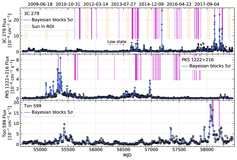
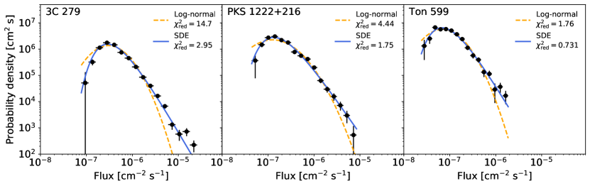
Refer to caption — Figure 1: Fermi-LAT light curves of 3C 279 (top), PKS 1222+216 (middle), and Ton 599 (bottom). The flux points (black circles) are shown for 1, 3, and 7 day time bins for the three sources, respectively. $5\,\sigma$ Bayesian blocks are shown with blue lines. The time intervals in which VERITAS observed the sources are marked in magenta. For 3C 279, time intervals in which the Sun is less than $20^{\circ}$ from the source are shown in orange and a Fermi-LAT low state from MJD 56230 – 56465 (see Section 6) is marked with a dashed line.

The distribution of the LAT fluxes observed from each of these FSRQs may provide a clue to the origin of the gamma-ray emission. The observed flux distributions of the three sources (scaled to form probability density histograms) are shown in Figure 2. Time bins that have a test statistic (TS) less than 9 or that occur when the Sun is less than $20^{\circ}$ from the source were excluded.

To account for uncertainties from both the flux binning and the finite observation length, the flux histogram bin errors were calculated using a bootstrapping approach. 2,500 bootstrap samples were used, each consisting of the same number of flux points as the actual light curve. Each bootstrap sample was obtained by sampling from the set of actual flux points with replacement, so that a given flux point might be sampled multiple times or not at all.

In order to include the uncertainties of the individual flux points, an error term was added to each sampled point in each bootstrap sample, determined by randomly sampling from a Gaussian distribution with standard deviation equal to the measurement uncertainty of the respective sampled point. The bin errors were then defined as the standard deviations of the bin fluxes over all of the bootstrap samples binned using the same bins as the original dataset.

One form of flux distribution often used to describe blazars is the log-normal distribution (Giebels09; Sinha17; Shah2018). Log-normal distributions are of interest because they indicate the presence of an underlying multiplicative rather than additive physical process (Aitchison1973). Light curves with a log-normal flux distribution have an amplitude of variability linearly proportional to their mean flux.

On the other hand, Tavecchio2020 have proposed an alternative model based on an SDE with two terms modeling a deterministic tendency to return to equilibrium and stochastic fluctuations with amplitude proportional to the absolute flux level. The form of the SDE is motivated by an astrophysical scenario of stochastic disturbances perturbing a magnetically arrested accretion disk. In this model, the flux distribution is asymmetrical about a peak, falling off as a power law at high fluxes and exponentially at low fluxes, with the relative importance of the deterministic and stochastic components dictating the shape of the distribution. Figure 2 shows a comparison between the best-fit probability density functions (PDFs) corresponding to a log-normal distribution and the stationary state of the SDE proposed by Tavecchio2020.

Table 2: Best-fit parameters and goodness of fit (

\chi^{2}_{\rm{red}}

) for the log-normal and SDE PDF fits to the LAT flux distributions. The mean

\mu

and standard deviation

\sigma

of the exponentiation of the log-normal distribution and the equilibrium flux

\mu

of the SDE distribution are normalized to

1\times 10^{-7}

ph cm

{}^{-2}

{}^{-2}

. The peak flux of the SDE PDF is given by

X_{\mathrm{max}}=\mu\lambda/(\lambda+2)

Source	Log-normal			SDE
	$\mu$	$\sigma$	$\chi^{2}_{\rm{red}}$	$\mu$	$\lambda$	$X_{\mathrm{max}}$	$\chi^{2}_{\rm{red}}$
3C 279	1.65 $\pm$ 0.02	0.73 $\pm$ 0.01	14.7	8.63 $\pm$ 0.28	1.01 $\pm$ 0.06	2.90 $\pm$ 0.21	2.95
PKS 1222+216	1.07 $\pm$ 0.03	0.92 $\pm$ 0.03	4.44	6.27 $\pm$ 0.60	0.54 $\pm$ 0.08	1.33 $\pm$ 0.23	1.75
Ton 599	0.21 $\pm$ 0.04	0.75 $\pm$ 0.03	1.76	2.11 $\pm$ 0.19	0.94 $\pm$ 0.15	0.68 $\pm$ 0.13	0.73

The stationary-state PDF corresponding to the SDE (Tavecchio2020, Appendix A) is

p(X)=\frac{(\lambda\mu)^{1+\lambda}}{\Gamma(1+\lambda)}\frac{e^{-\lambda\mu/X}}{X^{\lambda+2}},

(1)

where $X$ is a dimensionless random variable proportional to the flux, $\mu$ is a parameter representing the equilibrium value of $X$ , $\lambda$ is a parameter representing the relative weight of the deterministic and stochastic terms, and $\Gamma$ is the gamma function. Here, $X$ was related to the flux by a proportionality constant of $1\times 10^{-7}$ ph cm ${}^{-2}$ s ${}^{-1}$ . The distribution peaks at $X_{\mathrm{max}}=\mu\lambda/(\lambda+2)$ . The stationary-state PDF is valid on timescales much longer than the timescale for the system to return to equilibrium, which is clearly the case for the ten-year periods considered here.

The PDFs were fit to the histogram bins using a nonlinear least-squares algorithm. The best-fit parameters and reduced $\chi^{2}$ values of the two models are reported in Table 2. In all three cases, the SDE PDF provides a better fit than the log-normal PDF. Both models have two free parameters. We verified that the preference for the SDE model is preserved if the histogram bins at the lowest fluxes, which might be affected by requiring light curve bins to have TS $>9$ , are excluded from the fit.

The SDE model PDF is parameterized by the shape parameter $\lambda\equiv 2\theta/\sigma^{2}$ , where $\theta$ and $\sigma$ are the coefficients of the deterministic and stochastic terms. These parameters can be interpreted by associating $1/\theta$ with the timescale of magnetic field accumulation in the accretion disk, while $\sigma$ is related to the dynamics of the perturbative processes. A large value of $\lambda$ therefore represents a high relative importance of the deterministic variability component compared to the stochastic one, while a small value indicates the opposite. To relate these timescales to the gravitational radii of the central supermassive black holes, $r_{g}=GM/c^{2}$ , we adopt values of ${\sim}5\times 10^{8}$ , $6\times 10^{8}$ , and $3.5\times 10^{8}M_{\odot}$ for the black hole masses of 3C 279, PKS 1222+216, and Ton 599, respectively (Hayashida2015; Farina2012; Liu2006).

One can estimate $\sigma^{2}$ from the light curve using the expression (Tavecchio2020):

\sigma^{2}\simeq\frac{1}{n}\sum_{i=0}^{n}\frac{(X_{i}-X_{i-1})^{2}}{X_{i-1}^{2}(t_{i}-t_{i-1})},

(2)

where $X_{i}$ is the scaled flux at time step $i$ . Using this expression, we obtain $\sigma^{2}$ equal to 0.35, 0.16, and 0.062 day ${}^{-1}$ , or 100, 200, and 800 $r_{g}/c$ , for 3C 279, PKS 1222+216, and Ton 599, respectively. These values are consistent with the ${\gtrsim}100~{}r_{g}/c$ variability timescale injected into the jet by magneto-rotational instability in the accretion disk estimated in theoretical work (Giannios2019). Using the relation $1/\theta=2/\lambda\sigma^{2}$ , we can then constrain the physics of accretion flow in 3C 279, PKS 1222+216, and Ton 599 by estimating their magnetic flux accumulation timescales to be 200, 700, and 1800 $r_{g}/c$ , respectively, within the magnetically-arrested disk scenario.

4 Flare Selection

Flare states were identified in the Fermi-LAT data using the following procedure:

1.

Segment the data using Bayesian blocks. We set the false positive rate $p_{0}$ to the value equivalent to $5\,\sigma$ using Equation 13 of Scargle13.
2.

Choose a flux threshold above which the blocks are designated as flaring.
3.

Designate each contiguous set of flare blocks as an individual flare state and all non-flare blocks as the quiescent state.

This empirical procedure reflects a picture of individual flares superimposed on a constant quiescent background, but identifies them purely as states of elevated flux, making no explicit assumptions about the flares’ shape or spectra. Due to its basis on Bayesian blocks, it guarantees that states identified as flares have flux significantly greater than the states surrounding them.

The flux threshold to identify flares must be tuned on a source-by-source basis. Choosing the flux threshold to identify flares involves a trade-off between ensuring that dimmer flares are selected and avoiding misidentifying fluctuations in the quiescent background as flares. In addition, because the sources differ in average flux, the threshold must necessarily vary on an absolute level from source to source. Performing the flare selection procedure with the flare selection thresholds listed in Table 1 results in 10 flares selected for 3C 279, 11 for PKS 1222+216, and 5 for Ton 599, listed in Table 3. We set the threshold low enough for each source to ensure that all flares that triggered VERITAS observations were selected.

Table 3: Fermi-LAT flares selected using the algorithm given in Section 4. For each enumerated flare, the date range in MJD, approximate calendar date, number of Bayesian blocks, and amount of VHE gamma-ray exposure taken by VERITAS (if any) are provided. All of the times in the date ranges given in Table 1 but not listed here are considered to be quiescent.

#	Date Range (MJD)	Approx. Date	Blocks	VHE Exp.
3C 279
1	56645.66 - 56647.66	Dec 2013	1	-
2	56717.66 - 56718.66	Mar 2014	1	-
3	56749.66 - 56754.66	Apr 2014	1	6.79 hr
4	57186.66 - 57190.66	Jun 2015	3	1.00 hr
5	58116.66 - 58119.66	Dec 2017	1	-
6	58130.66 - 58141.66	Jan 2018	4	1.38 hr
7	58168.66 - 58173.66	Feb 2018	1	-
8	58222.66 - 58230.66	Apr 2018	5	0.83 hr
9	58239.66 - 58247.66	May 2018	1	-
10	58268.66 - 58275.66	Jun 2018	2	3.95 hr
PKS 1222+216
1	55096.66 - 55114.66	Sep-Oct 2009	3	-
2	55144.66 - 55201.66	Nov-Dec 2009	5	-
3	55231.66 - 55594.66	2010	27	-
4	55603.66 - 55639.66	Feb-Mar 2011	4	5.38 hr
5	55777.66 - 55783.66	Aug 2011	1	-
6	56494.66 - 56500.66	Jul 2013	1	-
7	56536.66 - 56665.66	Sep 2013	5	-
8	56680.66 - 56752.66	Jan-Apr 2014	3	15.53 hr
9	56926.66 - 57004.66	Sep-Dec 2014	5	-
10	58243.66 - 58249.66	May 2018	1	-
11	58321.66 - 58327.66	Jul 2018	1	-
Ton 599
1	55417.66 - 55445.66	Aug-Sep 2010	1	-
2	57342.66 - 57356.66	Nov 2015	1	-
3	57944.66 - 57958.66	Jul 2017	1	-
4	58042.66 - 58140.66	Oct 2017 - Jan 2018	5	8.30 hr
5	58217.66 - 58266.66	Apr-May 2018	1	2.00 hr

Because the flux distributions are best fit by the single-component SDE model PDF, it is not natural to calculate a duty cycle of flares based on a division into baseline and flaring components (e.g. Resconi2009). The amount of time spent in the highest-flux states can be estimated directly from the flux distribution by defining the “typical” flux as the peak of the PDF, given in Table 2. 3C 279, PKS 1222+216, and Ton 599 have flux greater than 5 (10) times the typical flux 12% (4%), 19% (8%), and 13% (4%) of the time, respectively.

Our flare selection flux thresholds for 3C 279 and Ton 599 are comparable at 13.8 and 11.8 times their typical fluxes, consistent with their similar values of the PDF shape parameter $\lambda\approx 1$ . For PKS 1222+216, our threshold is 3.8 times the typical flux. This source has a lower value of $\lambda\approx 0.5$ , with a correspondingly harder power law of the flux distribution at high fluxes. This is perhaps reflected in the long epochs of high flux seen in this source’s light curve, such as its Flare 3 in 2010 which is approximately a year in duration (Table 3). A relatively low threshold was therefore needed to also capture the smaller flares of the approximately weekly timescales that typically trigger VERITAS observations, consistent with the other two sources.

5 Daily and sub-daily variability

In order to deduce the smallest variability time around the rising and decaying periods of each flare selected according to the algorithm described in Section 4, we extracted sub-daily light curves of the three sources in time bins ranging from 12 hours down to 1.5 hours for the brightest source, 3C 279. Starting from daily time bins, we refined the light curve iteratively by splitting the time bin duration until each bin had a TS of $\gtrsim 50$ or until further refinement would not change the local trend of the light curve. For PKS 1222+216 and Ton 599, the minimum bin sizes were 12 and 6 hours, respectively.

To characterize the flares with multiple peaks we used a sum of exponential profiles (Valtaoja1999; Abdo2010), $F_{i}$ , where each one has the form:

F_{i}(t)=\begin{cases}F_{0_{i}}\,e^{(t-t_{\rm{peak}_{i}})/t_{\rm{rise}_{i}}},&t\leq t_{\rm{peak}_{i}}\\ F_{0_{i}}\,e^{-(t-t_{\rm{peak}_{i}})/t_{\rm{decay}_{i}}},&t>t_{\rm{peak}_{i}}.\end{cases}

(3)

For flares with a single peak we used:

F(t)=\begin{cases}F_{0}\,e^{(t-t_{\rm{peak}})/t_{\rm{rise}}}+F_{\mathrm{const}},&t\leq t_{\rm{peak}}\\ F_{0}\,e^{-(t-t_{\rm{peak}})/t_{\rm{decay}}}+F_{\mathrm{const}},&t>t_{\rm{peak}},\end{cases}

(4)

including a constant term to avoid having a bias towards large rise and decay timescales, which is minimal when multiple peaks are included.

The fitting procedure started by considering a single peak characterized by Equation (4). In order to evaluate the possibility of adding a second peak, a fit to the sum of two exponential profiles, as given by Equation (3), was performed and compared against the one-peak scenario using the reduced $\chi^{2}$ method. The two-peak model was then taken when an improvement was observed over the one-peak function. More peaks were then added following a similar procedure until a reasonable reduced $\chi^{2}$ value was reached, or when the best fit values obtained no longer provided relevant information for constraining the variability timescales of the sources under study. At each step, human judgment was used to initialize the profile positions and determine by eye that the fits made sense. The peaks were not required to match the Bayesian blocks used for flare selection, which were defined using the coarsely binned light curves.

The flare profiles of the three sources are shown in Figure 3. Two selected flares of 3C 279 are shown, as are the two flares each of PKS 1222+216 and Ton 599 that were observed by VERITAS. Profiles of all ten flares of 3C 279 are provided in Appendix LABEL:appendix:3c279flareprofiles. In order to illustrate when VERITAS observed the source relative to the LAT flare peaks, the VERITAS daily-binned light curves for each of the flares are also shown in Figure 3.

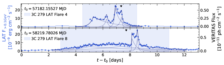
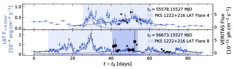
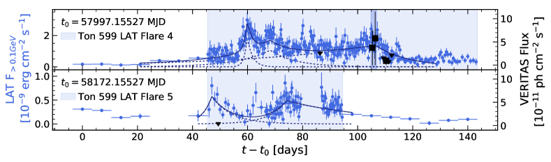
The fit results for the three sources are reported in Tables 4, 5, and LABEL:tab:flareprofile_3C279. For 3C 279, each flare lasted between one and eleven days and consisted of between one and four separately resolved components, modeled using exponential profiles. Twenty-four distinct components are resolved within the ten flares. The rise and decay times range from timescales of days to less than one hour. The smallest resolved variability timescale was $36\pm 13$ minutes, which occurred around MJD 58227.945, during the rising period of Flare 8 (MJD 58222.655 – 58230.655), indicated in boldface in Table 4 and Table LABEL:tab:flareprofile_3C279.

Table 4: Results of the LAT flare profile fits for 3C 279, with flare timescales in minutes.

	Amplitude ( $F_{0}$ )	$t_{\rm{peak}}$	$t_{\rm{rise}}$	$t_{\rm{decay}}$
	( $10^{-9}$ erg cm ${}^{-2}\,$ s ${}^{-1}$ )	(MJD)	(min)	(min)
Flare 4 (MJD 57186.655 – 57190.655): $\chi^{2}/$ d.o.f.= 77.31/19 = 4.07
	12.07 $\pm$ 0.67	57187.446 $\pm$ 0.031	378 $\pm$ 46	1784 $\pm$ 147
	09.79 $\pm$ 2.29	57188.425 $\pm$ 0.028	216 $\pm$ 101	155 $\pm$ 64
	21.72 $\pm$ 1.59	57189.069 $\pm$ 0.008	137 $\pm$ 18	512 $\pm$ 55
	12.41 $\pm$ 1.30	57189.532 $\pm$ 0.010	220 $\pm$ 63	77 $\pm$ 25
Flare 8 (MJD 58222.655 – 58230.655): $\chi^{2}/$ d.o.f.= 177.25/106 = 1.67
	05.29 $\pm$ 1.29	58224.773 $\pm$ 0.105	1996 $\pm$ 716	5899 $\pm$ 4035
	17.70 $\pm$ 2.01	58227.945 $\pm$ 0.004	36 $\mathbf{\pm}$ 13	329 $\pm$ 131
	16.42 $\pm$ 1.87	58228.323 $\pm$ 0.012	140 $\pm$ 54	115 $\pm$ 48
	05.59 $\pm$ 1.69	58227.139 $\pm$ 0.133	3816 $\pm$ 1450	4077 $\pm$ 2080

Note. — The smallest variability time found is indicated in boldface.

Table 5: Results of the LAT flare profile fits for PKS 1222+216 and Ton 599, with flare timescales in days.

	Amplitude ( $F_{0}$ )	$t_{\rm{peak}}$	$t_{\rm{rise}}$	$t_{\rm{decay}}$
	( $10^{-9}$ erg cm ${}^{-2}\,$ s ${}^{-1}$ )	(MJD)	(days)	(days)
PKS 1222+216
Flare 4 (MJD 55603.7 – 55639.7): $\chi^{2}/$ d.o.f.= 102.25/69 = 1.48
	0.56 $\pm$ 0.09	55607.1 $\pm$ 0.3	1.5 $\pm$ 0.5	2.7 $\pm$ 0.8
	0.48 $\pm$ 0.03	55629.9 $\pm$ 1.2	22.3 $\pm$ 3.5	12.1 $\pm$ 2.2
Flare 8 (MJD 56680.7 – 56752.7): $\chi^{2}/$ d.o.f.= 166.40/104 = 1.60
	0.72 $\pm$ 0.09	56692.9 $\pm$ 0.1	13.6 $\pm$ 2.7	0.4 $\pm$ 0.3
	1.75 $\pm$ 0.17	56702.8 $\pm$ 0.2	3.6 $\pm$ 0.6	1.5 $\pm$ 0.3
	0.43 $\pm$ 0.05	56721.9 $\pm$ 1.6	19.9 $\pm$ 8.5	10.4 $\pm$ 6.2
	0.41 $\pm$ 0.10	56732.0 $\pm$ 0.4	0.9 $\pm$ 0.8	8.6 $\pm$ 3.6
	0.44 $\pm$ 0.06	56746.9 $\pm$ 0.1	0.3 $\pm$ 0.3	10.3 $\pm$ 2.5
Ton 599
Flare 4 (MJD 58042.7 – 58140.7): $\chi^{2}/$ d.o.f.= 456.78/296 = 1.54
	1.89 $\pm$ 0.29	58057.1 $\pm$ 0.2	1.1 $\pm$ 0.3	1.9 $\pm$ 0.6
	1.06 $\pm$ 0.11	58065.4 $\pm$ 1.0	11.9 $\pm$ 2.6	9.0 $\pm$ 2.1
	1.37 $\pm$ 0.06	58103.5 $\pm$ 0.8	47.0 $\pm$ 4.7	11.8 $\pm$ 1.1
Flare 5 (MJD 58217.7 – 58266.7): $\chi^{2}/$ d.o.f.= 153.01/96 = 1.59
	0.57 $\pm$ 0.12	58219.2 $\pm$ 1.3	3.5 $\pm$ 2.8	7.3 $\pm$ 2.1
	0.48 $\pm$ 0.03	58246.3 $\pm$ 0.7	6.6 $\pm$ 1.7	34.9 $\pm$ 5.6

Note. — The flare components coincident with VHE flares are marked with a *, with corresponding smallest variability times indicated in boldface.

For PKS 1222+216 and Ton 599, the variability timescales were of the order of days. Notably, for both sources, the fastest variability did not occur during the detected VHE flares. The shortest variability timescale observed by LAT during the VHE flare of PKS 1222+216 was $10.4\pm 6.2$ days, which was the decay timescale of the coincident flare component. The shortest variability timescale of Ton 599 observed by LAT during its VHE flare was $11.8\pm 1.1$ days, which also was the coincident flare component’s decay timescale. In the case of Ton 599, the VERITAS detection occurred over a period of 2 days, after which the observed VHE flux became insignificant. No significant intra-flare variability was observed by Fermi-LAT or VERITAS during either event. Therefore, in the remainder of this work, we take the most constraining variability timescales during the VHE flares of PKS 1222+216 and Ton 599 to be 10 and 2 days, respectively.

The symmetry or asymmetry of flares can provide information on the timescales of the particle acceleration and cooling processes in the emission region (e.g. Abdo2010). If the cooling time is longer than the light travel time through the emission region, the decay time will be longer than the rise time, producing an asymmetric flare. If the cooling time is shorter than the light travel time, the flare will appear more symmetrical. Flares with a slow rise and fast decay may be produced by relativistic magnetic reconnection (Petropoulou2016).

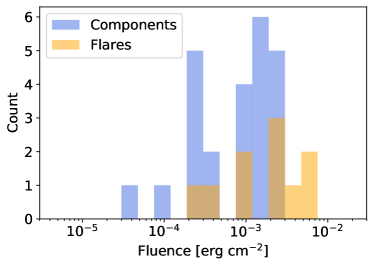
Figure 4 shows the fitted rise and decay times for each of the exponential flare components of 3C 279. No clear trend in the flare asymmetry is observable, whether overall, among components within a single flare, or between the components belonging to different flares. Both longer decay times and longer rise times are observed, and many flares appear symmetric. A Wilcoxon signed-rank test (Wilcoxon1945) finds no significant preference ( $p=0.178$ ) for flares to have a faster rise time than decay time rather than the reverse. These findings are consistent with previous studies of gamma-ray flares in bright Fermi blazars (e.g. Abdo2010; Roy2019).

Models of blazar flares powered by relativistic reconnection predict that flare components produced by large, non-relativistic plasmoids should have similar fluences to components produced by small, relativistic ones, so that flare components should have similar fluence regardless of their variability timescales (Petropoulou2016). Figure 5 shows the distributions of fluences of the components of the ten flares and the twenty-four individual flare components of 3C 279. The fluence $\mathcal{F}$ of a flare with exponential components $F_{i}$ is given by:

\mathcal{F}=\sum_{i}F_{0_{i}}(t_{\mathrm{rise}}+t_{\mathrm{decay}}).

(5)

For 3C 279 Flares 1, 2, 5, and 7, the best fit is given by a single component plus a constant baseline flux. In these cases, the baseline flux is included in the fluence estimate for consistency with the other flares, approximating the flare duration as $t_{\mathrm{rise}}+t_{\mathrm{decay}}$ , so that the fluence is given by:

\mathcal{F}=(F_{0}+F_{\mathrm{const}})(t_{\mathrm{rise}}+t_{\mathrm{decay}}).

(6)

The median flare fluence is $2.1\times 10^{-3}$ erg cm ${}^{-2}$ and the median component fluence is $0.85\times 10^{-3}$ erg cm ${}^{-2}$ . The observed component fluences range over about one order of magnitude, as do the flare amplitudes, while the rise and decay timescales span about two orders of magnitude. These dynamic ranges are generally compatible with the expectations for plasmoid-powered flares derived from particle-in-cell simulations of relativistic magnetic reconnection (Petropoulou2016).

The long-term gamma-ray variability study of the three FSRQs presented here is compatible with the extensive flare characteristics study carried out recently by Meyer2019 on the brightest flares detected by Fermi-LAT. A similar Bayesian blocks analysis was carried out to identify flares and look for variability on sub-hour timescales. Consistent with their findings, we find sub-hour-scale variability in 3C 279, where it was possible to resolve flares in finer time bins, suggesting that extremely compact emission regions may be present within the jet.

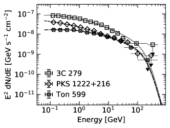
6 Gamma-ray Spectra

Figure 6 shows the LAT energy spectra corresponding to the entire data sets of each of the three sources, along with the VERITAS spectral upper limits for 3C 279. The best-fit spectral parameters are reported in Appendix LABEL:appendix:spectral_fit_parameters. Since all three sources were best fit by a log-parabola model in the 4FGL catalog (Abdollahi2020), we fit the LAT spectra with this model, parametrized as

\frac{dN}{dE}=N_{0}\left(\frac{E}{E_{b}}\right)^{-(\alpha+\beta(\log(E/E_{b}))},

(7)

where $E_{b}$ was fixed to the FL8Y catalog value of 457.698 MeV.

We checked that the log-parabola model provides a better fit than a power-law model using the likelihood ratio test. A power-law sub-exponential cutoff model was also preferred over a power law, but we could not establish whether this model is significantly preferred with respect to the log-parabola model using a likelihood ratio test. This is because the two curved models are non-nested, i.e. neither is a special case of the other, and therefore it is not possible to calculate the statistical significance of a preference for one over the other. We assumed a log-parabola spectrum for all subsequent LAT analyses. To facilitate comparison with the VERITAS points, the LAT model fits and butterfly contours were extended beyond the LAT maximum energy of 500 GeV, and extragalactic background light absorption was applied to them using the model of Franceschini_2017.

The global spectral shapes of the three sources are similar, with an index $\alpha$ of ${\sim}$ 2.1–2.3 and a curvature parameter $\beta$ of ${\sim}$ 0.04–0.06, and they differ primarily by their normalization.

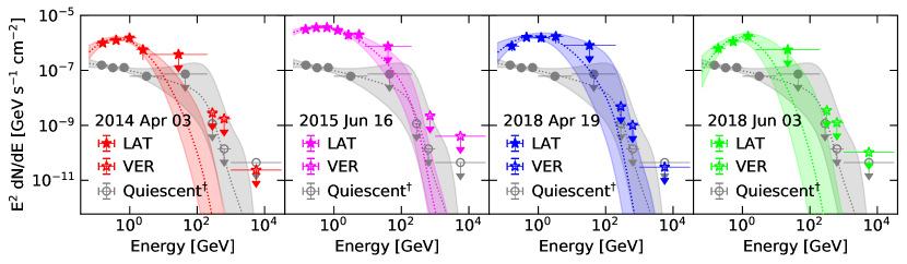
Using the data from 3C 279, we compared several methods to determine a baseline non-flaring spectrum. First, we defined a low state lasting from MJD 56230 to 56465 (see Figure 1), during which the flux was quiescent and stable in HE gamma rays, $R$ -band optical, and X-rays. We checked publicly available Tuorla⁴⁴4https://users.utu.fi/kani/1m/3C˙279˙jy.html data for the $R$ -band light curve. For the X-rays, we analyzed the Swift-XRT light curve using the online data products generator⁵⁵5https://www.swift.ac.uk/user˙objects/. To ensure low, stable gamma-ray emission, we selected the interval to span the Bayesian blocks with the lowest flux while excluding intervals with the Sun in the ROI. The low-state LAT SED is shown in Figure 6. Only one VERITAS observation occurred during this interval, on MJD 56417, so the corresponding VERITAS upper limits are not constraining and are not shown.

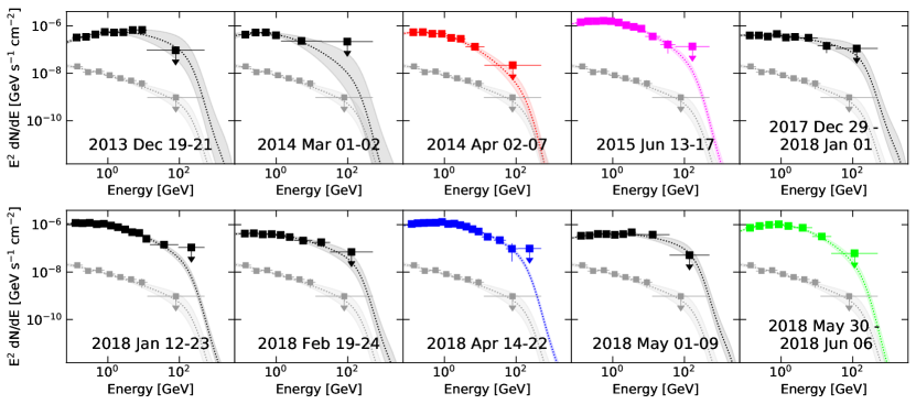
Next, using the algorithm proposed in this work and described in Section 4, we designated all epochs of the LAT light curve other than the flaring episodes as quiescent. From those epochs, we extracted those LAT data strictly simultaneous with the VERITAS observations, integrating a total of 43.6 hours of observations. The resulting strictly simultaneous LAT spectrum and VERITAS spectral upper limits are shown in Figure 6. We then performed the same procedure for four flaring epochs during which a significant Fermi-LAT detection could be obtained strictly simultaneous with the VERITAS observations, which occurred on the nights of April 3, 2014; June 16, 2015; April 19, 2018; and June 3, 2018. These strictly simultaneous LAT and VERITAS SEDs are shown in Figure 7.

The spectral shapes of the 3C 279 low and quiescent states are similar to each other and to the global state, although the uncertainties on their fit parameters are high due to the low significance. The spectra differ primarily in their flux normalization. The normalization of the low state is lower than that of the global state by design, while the normalization of the strictly simultaneous quiescent state is higher. This could result from the timing of the VERITAS monitoring and triggered observations which often follow up on Fermi-LAT flares and may tend to catch mildly elevated activity in Fermi-LAT even if the source is not actually flaring.

Finally, we derived LAT SEDs for all of the ten identified flares of 3C 279, using the entire flare time periods, irrespective of strict simultaneity with VERITAS, shown in Figure 8. The average flare spectrum is more strongly curved than the global spectrum, with $\alpha=2.02\pm 0.01$ and $\beta=0.093\pm 0.008$ , compared to $\alpha=2.228\pm 0.004$ and $\beta=0.061\pm 0.003$ for the global state.

7 SED Modeling

Multiwavelength SED modeling can shed light on the mechanisms of gamma-ray production during VHE flares. For 3C 279, we refer the reader to those works in the literature in which multiwavelength SED modeling of the epochs considered here has been performed, and we do not perform any additional modeling (see for example, Hayashida2015; Ackermann2016; Prince2020; Yoo2020).

PKS 1222+216 was first detected at TeV energies by MAGIC during a flaring event in June 2010 (Aleksic2011), and multiwavelength SED modeling of this event has been performed by e.g. Tavecchio2011. We therefore restricted our SED modeling of the source to the duration of the second VHE detection by VERITAS in February and March 2014. We considered data from all instruments taken from UT 2014-02-26 to 2014-03-10, inclusive.

Ton 599 has not been studied as extensively as the other two sources. Prince2018 and Patel2020 model its variability characteristics and multiwavelength SED, respectively, during the high state in December 2017, but do not have access to TeV data. We therefore modeled the multiwavelength SED of Ton 599 during the VERITAS detection in December 2017. We considered data from all instruments taken from UT 2017-12-15 to 2017-12-16, inclusive.

To assemble our multiwavelength SEDs, in addition to the gamma-ray data from VERITAS and Fermi-LAT, we incorporated X-ray and ultraviolet data from the XRT and UVOT instruments aboard the Swift satellite and optical observations from the Steward Observatory.

We described the multiwavelength SEDs of the two FSRQs using a multi-component synchrotron self-Compton (SSC) blob-in-jet model, implemented using the framework of the “Bjet” code, developed by Hervet2015 and based on Katarzynski2001. We modeled the radiative interactions of a compact leptonic emission zone (a blob), including an EIC emission component resulting from the interactions of the blob particles with the thermal accretion disk emission reprocessed by the BLR. Figure 9 shows a schematic illustration of the components producing the emission in this model.

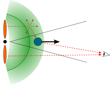
We consider a simplified BLR model with a normalized density profile, based on Nalewajko2014, where $\rho_{\mathrm{BLR}}(r)$ is at a maximum at the characteristic BLR radius $r=r_{\mathrm{BLR}}$ and decreasing as $r^{-2}$ with the distance to the core such that

\rho_{\mathrm{BLR}}(r)=\frac{(r/r_{\mathrm{BLR}})^{2}}{1+(r/r_{\mathrm{BLR}})^{4}}~{},

(8)

with $r_{\mathrm{BLR}}$ scaled to the bolometric disk luminosity $L_{d}$ as $r_{\mathrm{BLR}}=0.1\sqrt{L_{d}/1\times 10^{46}~{}\mathrm{erg}~{}\mathrm{s}^{-1}}$ pc (Sikora2009; Ghisellini2009). From SED modeling of PKS 1222+216 and Ton 599 we deduce a BLR radius of 0.17 pc and 0.15 pc respectively. We assume an isotropic diffusion of the disk light by the BLR, where the specific intensity of this field can be expressed as

I_{\mathrm{BLR}}(\nu,T_{d},r)=\epsilon_{\mathrm{BLR}}\rho_{\mathrm{BLR}}(r)\frac{L_{d}}{4\pi r^{2}}\frac{I_{p}(\nu,T_{d})}{(\sigma_{\mathrm{SB}}/\pi)T_{d}^{4}},

(9)

where $\sigma_{\mathrm{SB}}$ is the Stefan-Boltzmann constant, $I_{p}$ is the Planck intensity, and $\epsilon_{\mathrm{BLR}}$ is the covering factor. This equation is similar to Eq. 12 in Hervet2015 with the addition of the BLR density profile. Only the extension of the BLR in front of the blob plays a significant role in our modeling since it drives the number of gamma rays produced by the blob that will be absorbed by pair production. The BLR is by default defined between $r=0$ and $r=100~{}r_{\mathrm{BLR}}$ . Given the fast convergence of the BLR opacity ( $I_{\mathrm{BLR}}\propto r^{-4}$ ), the maximum extension of the BLR does not play a significant role in the model. Although we assume for simplicity that the BLR is isotropic, any anisotropy should have a small effect on the opacity (e.g. Abolmasov2017, Figure 14).

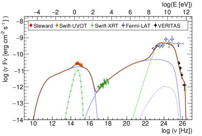
Figures 10 and 11 show the multiwavelength SED models of PKS 1222+216 and Ton 599. In these figures, the synchrotron and SSC emission are shown by solid blue lines. The subdominant second-order self-Compton emission caused by the interactions of the electrons with the self-Compton photons is shown by a dotted blue line. The thermal emission from the accretion disk is modeled as a point source radiating as a black body, and is shown by a heavy dashed green line. The inverse Compton emission due to the interaction of the electrons with the disk photons reprocessed in the BLR is shown by a dashed green line. Table 6 gives the parameters characterizing the SED models.

Our model does not include any secondary radiation from pair cascades produced by the absorption of gamma rays in the BLR. While detailed modeling of this effect is beyond the scope of this paper, we estimate that the potential contribution of such cascades would be $\ll 1\%$ of the total bolometric luminosity for PKS 1222+216 and $\lesssim 1\%$ for Ton 599, given the respective levels of absorption in our models, which are described below. We evaluated these contributions by comparing the radiative output of each model with that from the same model with the BLR opacity set to zero. This effect may be noted as a source of systematic uncertainty when interpreting our results.

We note that our model requires that the dust-torus luminosity be negligible compared to the disk luminosity. As evidence of far-infrared dust-torus thermal emission is lacking in the SED, we consider this assumption to be reasonable in our study. Observing campaigns with good microwave to IR coverage would be needed to fully confirm this approach. The presence of strong dust-torus emission would require that the gamma-ray emission zone be farther downstream in the jet so as not to produce too large an opacity by pair production.

7.1 PKS 1222+216 modeling

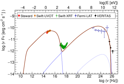
In order to investigate the necessity of including an EIC component, we represented the multiwavelength SED of PKS 1222+216 with a one-zone pure SSC model, shown in Figure 10 (left). As can be seen by the similar amplitudes of the synchrotron and inverse Compton peaks in the figure, the SED is only weakly Compton dominated, with the inverse Compton luminosity about twice the synchrotron luminosity. The Swift-XRT spectrum contains a well-resolved break showing the transition between synchrotron and inverse Compton dominated emission, which sets a strong constraint on the model. Our best attempt does not provide a satisfying representation of the observed SED. The main issue is that the optical-to-X-ray components of the SED have steep slopes which would require a narrow, sharp synchrotron bump to achieve a good representation, while the X-ray-to-VHE needs a wide, flat inverse Compton bump. This is not compatible with the usual simple SSC framework, especially when the SED is not heavily Compton dominated.

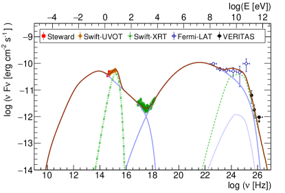
In our EIC model, the IR-to-UV SED is dominated by the blackbody big-blue-bump emission of an accretion disk (see Figure 10, right), which resolves the tension by eliminating the constraint on the synchrotron spectral shape. This allows for a broad SSC component matching the spectral break observed in the X-ray band. In this scenario, the VHE emission is produced by the EIC process between a relativistic blob and the disk thermal emission reprocessed by the BLR. The blob is set to a distance of 3.56 pc from the SMBH, corresponding to $21.3~{}r_{\mathrm{BLR}}$ . It should be noted that a thermal EIC process was also favored in previous models of PKS 1222+216 where clear disk emission and a strongly Compton-dominated SED were observed during a major outburst in 2010 (Tavecchio2011).

Because the peak frequency of the EIC emission is directly proportional to the blob Lorentz factor, this scenario imposes a strong constraint on the jet parameters. For PKS 1222+216, in order to match the VHE spectrum, the bulk Lorentz factor needs to be above approximately 23, which was achieved by assuming a Doppler factor $\delta=40$ and an angle with the line of sight $\theta_{\mathrm{obs}}=1\degree$ . This assumption is consistent with the jet constraints derived by Hervet_2016 from the fastest motion observed in the radio jet of PKS 1222+216, which led to estimations of $\theta_{\mathrm{obs}}=1.3\degree$ , $\delta=41.3$ and $\Gamma=29.2$ .

Because no significant variability was observed in any waveband during the time period selected for modeling for either source, we considered a stationary model giving a snapshot of the observed activity. As a consistency check, we compared the expected radiative cooling time from the model with the observed flare decay timescale. The cooling time associated with the full radiative output (synchrotron, SSC and EIC emissions) can be expressed in the Thomson regime as

T_{\mathrm{cool}}(\gamma)=\frac{3m_{e}c}{4\sigma_{T}\gamma(U^{\prime}_{B}+U^{\prime}_{\mathrm{syn}}+U^{\prime}_{\mathrm{blr}})},

(10)

with $m_{e}$ the electron mass, $\sigma_{T}$ the Thomson cross section, $\gamma$ the Lorentz factor of the emitting particle, and $U^{\prime}_{B}$ , $U^{\prime}_{\mathrm{syn}}$ , $U^{\prime}_{\mathrm{blr}}$ respectively the energy density in the blob frame of the magnetic field, synchrotron field, and external BLR field (e.g. Inoue_1996). One can associate the energy at the break of the spectral particle distribution $\gamma_{\mathrm{brk}}$ with the emission at the peaks of the SED. The Fermi-LAT energy range being mostly above this peak, we can deduce $T_{\mathrm{cool}}(\mathrm{\textit{Fermi}})\lesssim 17$ days. This is consistent with the observed Fermi-LAT flare decay of $10.4\pm 6.2$ days.

The minimum possible variability predicted by our model is 18 h, given by the blob’s radius and Doppler factor such that $\tau_{\mathrm{min}}=R(1+z)/(c\delta)$ . The total power of the jet is approximately $3.4\times 10^{45}$ erg s ${}^{-1}$ , in a particle-dominated regime with the equipartition parameter $U_{B}/U_{e}=1.7\times 10^{-3}$ .

7.2 Ton 599 modeling

Contrary to PKS 1222+216, the SED of Ton 599 is heavily Compton dominated, with a ratio of inverse Compton to synchrotron luminosity of approximately one order of magnitude. This is a usual signature of an EIC component dominating the gamma-ray emission. We therefore consider the same scenario as for PKS 1222+216. As shown in Figure 11, the model describes the data well.

As in the case of PKS 1222+216, the thermal EIC emission imposes strong constraints on the properties of the emitting region. The largest constraint comes from the gamma-ray opacity by pair creation from the luminous thermal field surrounding the blob. We found that only for a Doppler factor of ${\gtrsim}50$ is the EIC emission at VHE strong enough to produce the observed VHE gamma rays, given the BLR opacity.

Table 6: Parameters of the SED models.

Parameter	PKS 1222+216	Ton 599	Unit
$\theta_{\mathrm{obs}}$	$1.0$	$1.0$	deg
Blob
$\delta$	$40$	$53$
$N_{e}^{(1)}$	$2.0\times 10^{4}$	$2.7\times 10^{5}$	cm ${}^{-3}$
$n_{1}$	$2.1$	$2.5$	$-$
$n_{2}$	$3.9$	$3.0$	$-$
$\gamma_{\mathrm{min}}$	$5.5\times 10^{2}$	$3.0\times 10^{2}$	$-$
$\gamma_{\mathrm{max}}$	$3.0\times 10^{5}$	$7.0\times 10^{4}$	$-$
$\gamma_{\mathrm{brk}}$	$5.0\times 10^{3}$	$1.5\times 10^{4}$	$-$
$B$	$3.0\times 10^{-2}$	$3.0\times 10^{-2}$	G
$R$	$5.5\times 10^{16}$	$6.0\times 10^{16}$	cm
$D_{\mathrm{BH}}$ ^^ Host galaxy frame.	$3.56$	$2.33$	pc
Nucleus
$L_{\mathrm{disk}}$	$2.8\times 10^{46}$	$2.2\times 10^{46}$	erg s ${}^{-1}$
$T_{\mathrm{disk}}$	$2.8\times 10^{4}$	$1.1\times 10^{4}$	K
$\epsilon_{\mathrm{BLR}}$	$2.0\times 10^{-2}$	$2.0\times 10^{-2}$	$-$

Note. — $\theta_{\mathrm{obs}}$ is the angle of the blob direction of motion with respect to the line of sight. The electron energy distribution between Lorentz factors $\gamma_{\mathrm{min}}$ and $\gamma_{\mathrm{max}}$ is given by a broken power law with indices $n_{1}$ and $n_{2}$ below and above $\gamma_{\mathrm{brk}}$ , with $N_{e}^{(1)}$ the normalization factor at $\gamma=1$ . The blob Doppler factor, magnetic field, radius, and distance to the black hole are given by $\delta$ , $B$ , $R$ , and $D_{\mathrm{BH}}$ , respectively. The disk luminosity and temperature are given by $L_{\mathrm{disk}}$ and $T_{\mathrm{disk}}$ , while $\epsilon_{\mathrm{BLR}}$ is the covering factor of the broad line region.

The solution presented in Figure 11, with $\delta=53$ , is consistent with a maximum VHE emission undergoing strong BLR absorption ( $E_{\mathrm{max}}=630$ GeV), with an opacity of $\tau_{\gamma\gamma,E_{\mathrm{max}}}=2.8$ . In this scenario we set the blob at a distance of 2.33 pc from the SMBH, corresponding to $15.7~{}r_{\mathrm{BLR}}$ .

By applying the same consistency check for variability as PKS 1222+216, we found a minimal possible variability timescale predicted by the model of 18 h (coincidentally the same as PKS 1222+216), and a radiative cooling time $T_{\mathrm{cool}}(\mathrm{\textit{Fermi}})\simeq 8.7$ days, in good agreement with the observed Fermi-LAT flare decay of $11.8\pm 1.1$ days. The VERITAS observed variability can be associated with the cooling time $T_{\mathrm{cool}}(\gamma_{\mathrm{max}})$ , which leads to $T_{\mathrm{cool}}(\mathrm{VERITAS})=45$ h, fully compatible with the observed variability of $\sim$ 2 days. The blob is estimated to have a total power of approximately $1.2\times 10^{46}$ erg s ${}^{-1}$ , and to be extremely particle-dominated with equipartition parameter $U_{B}/U_{e}=3.8\times 10^{-4}$ .

Table 7: Parameters used to calculate constraints on the parameter space.

Source	z	$D_{L}$	$t_{\mathrm{var}}$	$L_{\mathrm{syn}}$	$L_{\mathrm{gamma}}$	$L_{d}$	$M_{\mathrm{BH}}$ ^a^aFarina2012; Liu2006	$E_{\mathrm{cool}}$	$\epsilon_{\mathrm{BLR}}$ ^b^bTavecchio2011	$\epsilon_{\mathrm{IR}}$ ^b^bTavecchio2011
		Gpc	day	erg s ${}^{-1}$	erg s ${}^{-1}$	erg s ${}^{-1}$	$M_{\odot}$	GeV
PKS 1222+216	0.434	2.44	10.0	$3.5\times 10^{46}$	$7.8\times 10^{46}$	$2.8\times 10^{46}$	$3.47\times 10^{8}$	7.07	0.02	0.2
Ton 599	0.725	4.54	2.0	$4.4\times 10^{46}$	$1.2\times 10^{48}$	$2.2\times 10^{46}$	$6.8\times 10^{8}$	326	0.02	0.2

Note. — $z$ and $D_{L}$ are the redshift and luminosity distance of the source. $t_{\mathrm{var}}$ is the variability timescale of cooling derived from each flare’s fitted exponential decay. $L_{\mathrm{syn}}$ , $L_{\mathrm{gamma}}$ , and $L_{d}$ are the synchrotron luminosity, gamma-ray luminosity, and disk luminosity from the SED model. $M_{\mathrm{BH}}$ is the black hole mass. $E_{\mathrm{cool}}$ is the maximum photon energy due to the external Compton cooling of relativistic electrons. $\epsilon_{\mathrm{BLR}}$ and $\epsilon_{\mathrm{IR}}$ are the covering factors of the broad line region and IR-emitting torus region, respectively.