Reconstructing Pruned Filters using Cheap Spatial Transformations

Abstract

We present an efficient alternative to the convolutional layer using cheap spatial transformations. This construction exploits an inherent spatial redundancy of the learned convolutional filters to enable a much greater parameter efficiency, while maintaining the top-end accuracy of their dense counter-parts. Training these networks is modelled as a generalised pruning problem, whereby the pruned filters are replaced with cheap transformations from the set of non-pruned filters. We provide an efficient implementation of the proposed layer, followed by two natural extensions to avoid excessive feature compression and to improve the expressivity of the transformed features. We show that these networks can achieve comparable or improved performance to state-of-the-art pruning models across both the CIFAR-10 and ImageNet-1K datasets.

1 Introduction

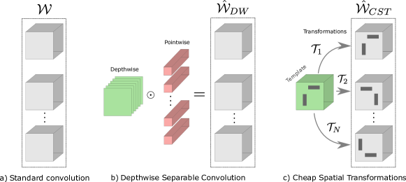
Figure 1: Constructing more convolutional filters using cheap spatial transformations. (a) Original convolutional layer. (b) Depth-wise separable layers, which fully decouple the spatial and depthwise aggregation of features. (c) Proposed layer expressed new filters as spatial transformations of a smaller set of templates.

Convolutional neural networks (CNNs) have achieved state-of-the-art results across a range of computer vision tasks [45, 6]. Despite their success, these models are typically far too large and computationally expensive for their deployment on resource constrained devices, such as mobile phones or edge devices. Recent work on compressing CNNs [28, 59, 51, 31, 7, 42, 15, 16], have exploited the inherent weight redundancy using structured pruning. This approach provides a way to reduce the size of a network without relying on sparse software libraries or hardware accelerators. Most of these methods involve ranking the importance of filters and then removing those that fall below a specific threshold. However, it is important to note that when the pruning rates are high, some of these pruned filters can still contribute in retaining the top-end accuracy. To address this limitation, we propose a cheap decomposition of the convolutional layer where the pruned filters are reconstructed using cheap spatial transformations of the non-pruned filters, which we call templates. We propose an approach to transfer an existing CNN to this efficient architecture through a generalised pruning pipeline. This methodology can be considered a natural extension of pruning, but instead of zeroing out the pruned filters, we are replacing them with the cheap template transformation. This work can be related to group equivariant convolutional networks [5], which consider the hand-crafted construction of filters using a pre-defined group to learn equivariant features. In contrast to this work, we jointly learn both the transformations and templates with the alternative objective of training small and efficient CNNs. Our contributions can be summarised as follows:

• We propose a novel approach to construct expressive convolutional filters from cheap spatial transformations using a set of filter templates.

• We model the training as a generalised pruning problem with a simple magnitude based saliency measure.

• We introduce a grouped extension to mitigates excessive feature compression.

• Our results show competitive performance over state-of-the-art pruning methods on both the CIFAR-10 and ImageNet-1K datasets.

1.1 Related work

The most relevant work can be divided into pruning, low-rank decomposition, and knowledge distillation.

Pruning explicitly exploits the inherent parameter redundancy by removing individual weight entries or entire filters that have the least contribution to the performance on a given task. This was first introduced in [26, 13] using the Hessian of the loss to derive a saliency measure for the individual weights. SNIP [27] proposed to prune weights using the connection sensitivity between individual neurons. Subsequent work propose a sparse neuron skip layer [46] to achieve fast training convergence and a high connectivity between layers. Cheap heuristic measures have also been used, such as the magnitude [12, 28], geometric median [15], or average percentage of zeros [20]. Although some of these unstructured pruning methods are able to achieve significant model size compression, the theoretical reduction in floating-point operations (FLOPs) does not translate to the same practical improvements without the use of dedicated sparse hardware and software libraries. This has led to the more widespread adoption of structured pruning approaches, which focus on removing entire filters. [59] introduced additional loss terms to select the channels with the highest discriminative power, while [55] proposed to prune in accordance with a neural importance score. DMCP [10] models the pruning operation as a differentiable markov chain, where compression is achieved through a sparsity inducing prior. Similarly, [1, 57] model pruning in the probabilistic setting using both hierarchical and sparsity inducing priors. Unlike these prior works, we propose to reconstruct the pruned filters using cheap transformations. These reconstructed filters are shown to be expressive and learn diverse features, thus mitigating the need for any sophisticated pruning strategies.

Low-rank decomposition is concerned with compactly representing a high-dimensional tensor, such as the convolutional weights, as linear compositions of much smaller, lower-dimensional, tensors, called factors. Any linear operations that are then parameterised by these weights can be expressed using cheaper operations with these factors, which can lead to a reduction in the computational complexity. Depthwise separable convolutions split the standard convolution into two stages, the first extracts the local spatial features in the input, while the second aggregates these features across channels. They were originally proposed in Xception [4] but have since been adopted in the design of a range of efficient models [2, 9, 19, 47]. This has led to the development of optimized GPU kernels that bridge the gap between the theoretical FLOP improvements and the practical on-device latency. Both CP-decomposition [18] and Tucker decomposition [49] have also been used to construct or compress pre-trained models [21, 23, 37]. Another line of work has explored the use of tensor networks as a mathematical framework for generalising tensor decomposition in the context of deep learning [14, 50]. Ghost modules [11] use depthwise convolutions to construct more features, leading to improved capacity at a much smaller overhead. Our proposed layer can be seen as an alternative parameterisation of the convolutional weights which can be naturally pruned using a generalised pruning pipeline.

Knowledge distillation attempts to transfer the knowledge of a large pre-trained model (teacher) to a much smaller compressed model (student). This was originally introduced in the context of image classification [17], whereby the soft predictions of the teacher can act as pseudo ground truth labels for the student. This methodology enables the student model to more easily learn the correlations between classes which are not available through the one-hot encoded ground truth labels. Hinted losses further provide knowledge distillation for the intermediate representation [43] and can be modelled as reconstruction L2 loss terms in the same space or in a projected feature space [52, 41, 39, 3, 36, 38]. Weight sharing and jointly training models at different widths/pruning-rates has also been shown to provide implicit knowledge distillation to the smallest models [54, 53]. In general, our proposed method is orthogonal to knowledge distillation - its adoption can be employed in addition to further improve performance.

2 Method

In this section we propose a novel decomposition of the convolutional layer. We do this be expressing the convolutional filters as spatial transformations of a compact set of template filters. These templates are obtained through a well-established pruning procedure, ensuring discriminative features. Subsequently, we present an algorithmically equivalent derivation of this layer that has much fewer floating-point operations (FLOPs). Moreover, we extend our approach naturally by introducing a group extension, which enhances the connectivity between layers. This extension enables an improved channel connectivity, fostering more robust and informative feature propagation.

2.1 Constructing diverse convolutional filters.

Let $\mathcal{W}=\{\mathcal{W}_{n}\in{\rm I\!R}^{K\times K\times C}\}_{n=1}^{N}$ describe the set of filters for a given convolutional layer with an input depth $C$, output depth $N$, and a receptive field size of $K\times K$. Our method is based on an assumption that a large subset of these filters can be faithfully approximated as spatial transformations of a much smaller set of filters, which we call templates $\mathcal{B}$. For simplicity, and without loss in generality, consider the scalar transformations, which can be implemented as cheap element-wise products between the spatial entries of the templates. Thus, for a $K\times K\times C$ template, each transformation can be parameterised using $K\times K$ learnable weights. Consider the case with $N$ templates and $N$ output feature maps. The proposed decomposition is given as follows:

$$\mathcal{Y}_{h,w,n} =\sum_{k_{w},k_{h}}^{K}\sum_{i}^{C}\mathcal{X}_{h^{\prime},w^{\prime},i}\cdot\mathcal{W}_{k_{h},k_{w},c,n}$$ (1)

$$\approx\sum_{k_{w},k_{h}}^{K}\sum_{i}^{C}\mathcal{X}_{h^{\prime},w^{\prime},i}\cdot\mathcal{B}_{k_{h},k_{w},i,n}\cdot\mathcal{T}_{k_{h},k_{w},n}$$ (2)

$$h^{\prime}=(h- 1)s+k_{h}-p,\;\;\;\;w^{\prime}=(w-1)s+k_{w}-p$$

where $s$ is the stride and $p$ is zero-padding. The general formulation using affine transformations is illustrated in figure 1. Model compression can be achieved when the number of basis filters $M$ is less than the number of output feature maps $N$. This is realised through pruning, which is discussed in second 2.2. In this case, the templates are then re-used to compute more filters using different transformations.

The choice of mapping from which template to which output feature map is not critical, as long as it is fixed after the pruning stage to enable fine-tuning. For our experiments, we set this mapping to be $i=j\;mod\;M$, where the $i$th output feature map is allocated the $j$th template, and where $M$ is the total number of templates. This choice of mapping ensures that all templates are uniformly used, thus enabling a diverse set of transformed filters. The spatial transformations are then jointly learned alongside the templates.

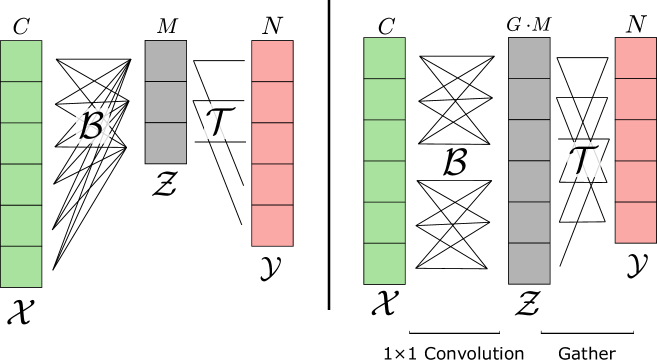
(a)

Figure 2: Too few templates can overly compress the input features. We propose to introduce a group parameter to naturally balance the expressiveness of the both the template and transformation stages.

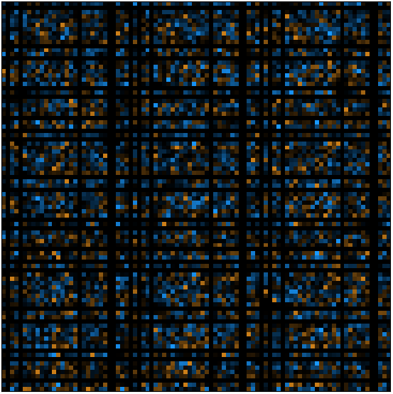
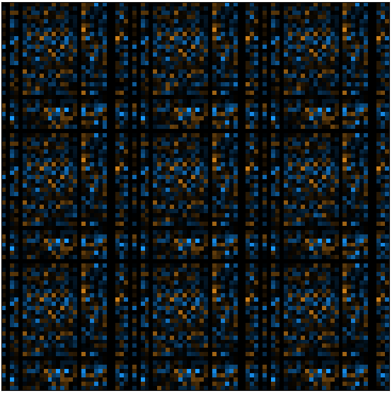
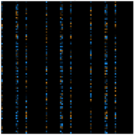
(a)

Figure 3: Visualising learned transformations for a given layer. (left) original learned filters. (middle) expressive filters using affine template transformations. (right) pruning filters. Both the vanilla pruned layer and the decomposed layers use a pruning rate of 0.7. Each column represents a filter for a given output channel and black pixels represent zero entries.

2.2 Using pruning to select the filter templates.

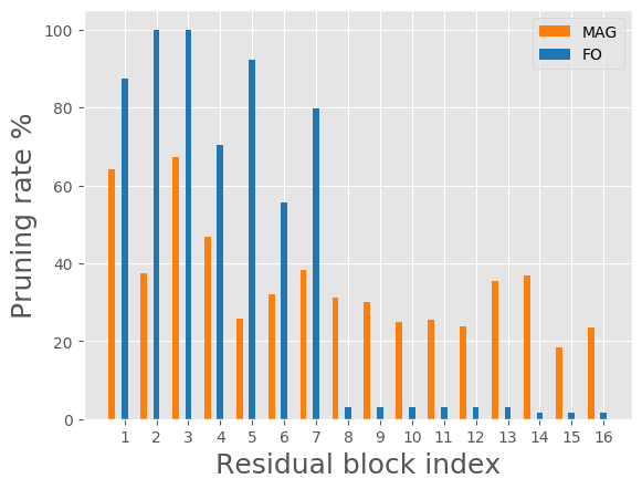
Figure 6: Comparing the pruning rates of each layer using different saliency measures. We see that a magnitude based (MAG) criterion exhibits a more uniform pruning rate than gradient based measures (FO).

The pruning literature has proposed increasingly sophisticated pruning heuristics and training pipelines. Examples of such including layer-wise pruning strategies [8] and gradient-based saliency measures [40], which incur additional hyperparameters and increased computational costs. In favour of simplicity, and to demonstrate the generalisability of our decomposition, we propose to use a very simple magnitude-based criterion to rank the importance of filters for selecting the set of templates. We observe that this choice of saliency measure naturally leads to a uniform pruning strategy across all layers in the network (figure 6), which reduces excessive feature compression for any given layer (see section 2.4).

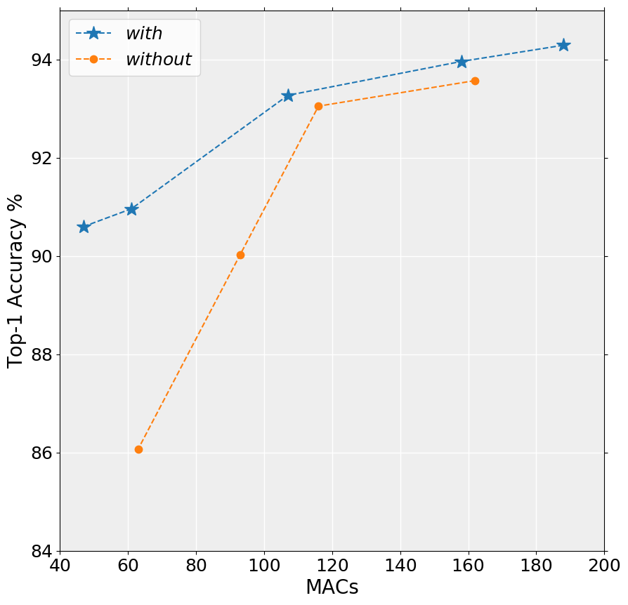
(a)

Figure 4: Comparison with a pruned baseline and the importance of which pruning heuristic. (left) Performance of a VGG16 network trained using affine (with) and scalar (without) spatial transformations with the same training methodology. (right) show the performance trade-off at different pruning rates using both a magnitude-based and a gradient-based saliency.

We provide an ablation on the importance on the choice of saliency measure in figure 4 (right). In this ablation we compare the performance using two different measures, namely magnitude based and gradient based [40]. Although in some cases the gradient based measure does lead to better performance, which is attributed to a more discriminative selection of templates, it does come at an increased computational overhead. In favour of simplicity, and to demonstrate the robustness to the choice of templates, we use a magnitude based measure throughout. In fact, for the ImageNet-1K experiments we extend this hypothesis and use a randomly initialised network to begin with, rather than from a pre-trained network - as is more commonly used in the pruning literature.

2.3 Performance and efficient implementations.

Computing the output features using the transformed filters and then using a standard convolution would not lead to any reduction in FLOPs. To address this, we propose to decompose the convolutional layer into two stages. The first computes the template features $\mathcal{Z}$ using the template filters $\mathcal{B}$, while the second projects these features to a different space using the spatial transformations $\mathcal{T}$. The output features are then the union of the original template features (identity transformations) and the transformed features. This two stage implementation is algorithmically equivalent to first constructing the filters and then performing a convolution, and its derivation is given as follows:

$$\mathcal{Y}_{h,w,n} \approx\sum_{k_{w},k_{h}}^{K}\sum_{i}^{C}\mathcal{X}_{h^{\prime},w^{\prime},i}\cdot\mathcal{B}_{k_{h},k_{w},i,n}\cdot\mathcal{T}_{k_{h},k_{w},n}$$ (3)

$$=\sum_{k_{w},k_{h}}^{K}\mathcal{T}_{k_{h},k_{w},n}\underbrace{\left(\sum_{i}^{C}\mathcal{X}_{h^{\prime},w^{\prime},i}\cdot\mathcal{B}_{k_{h},k_{w},i,n}\right)}_{\mathcal{Z}}$$ (4)

Computing $\mathcal{Z}$ can be achieved using a pointwise convolution, which translates to an optimised general matrix multiply primitive. The second stage, which consists of projecting $\mathcal{Z}$ to the output space, reduces to a series of gather operations and multiplications, which will implement the spatial transformations. Both of these operations can be trivially implemented in most deep learning frameworks.

2.4 Channel connectivity and feature compression.

By design, the proposed decomposition preserves the same number of input and output channels as the original convolution. This means that all the pruned filters are being reconstructed using some cheap and learned template transformation. The consequence of this design is that at high pruning rates there will be a significant bottleneck in the latent space $\mathcal{Z}$ (see figure 2). This bottleneck can result in significant feature compression that can degrade the downstream performance and discriminative power of representations. We could address this problem by simply increasing the number of templates per layer, but this would incur a significant overhead in terms of both parameters and FLOPs. Instead, we propose to introduce a grouped extension that can naturally scale the dimensionality of the latent space $\mathcal{Z}$ with a minimal computational and parameter overhead. To do this we replace the pointwise convolution in the two stage processing with a grouped pointwise convolution [25], which has an efficient implementation in most deep learning frameworks. This transformation then translates to the sum of $G$ transformations applied to feature maps from the $G$ distinct groups. Doing so in this way enables cross-group information flow without the need for any channel shuffles [56]. Figure 2 graphically demonstrates this grouped extension. On the left is the original case, whereby $G=1$. At this pruning rate, there is a very large compression of features. Increasing the groups to 2 (as shown on the right) provides a natural scheme for increasing the depth of $\mathcal{Z}$ without incurring any significant computational overhead. The results of the $G$ different transformations across groups are then added to form each of the $N$ output channels.

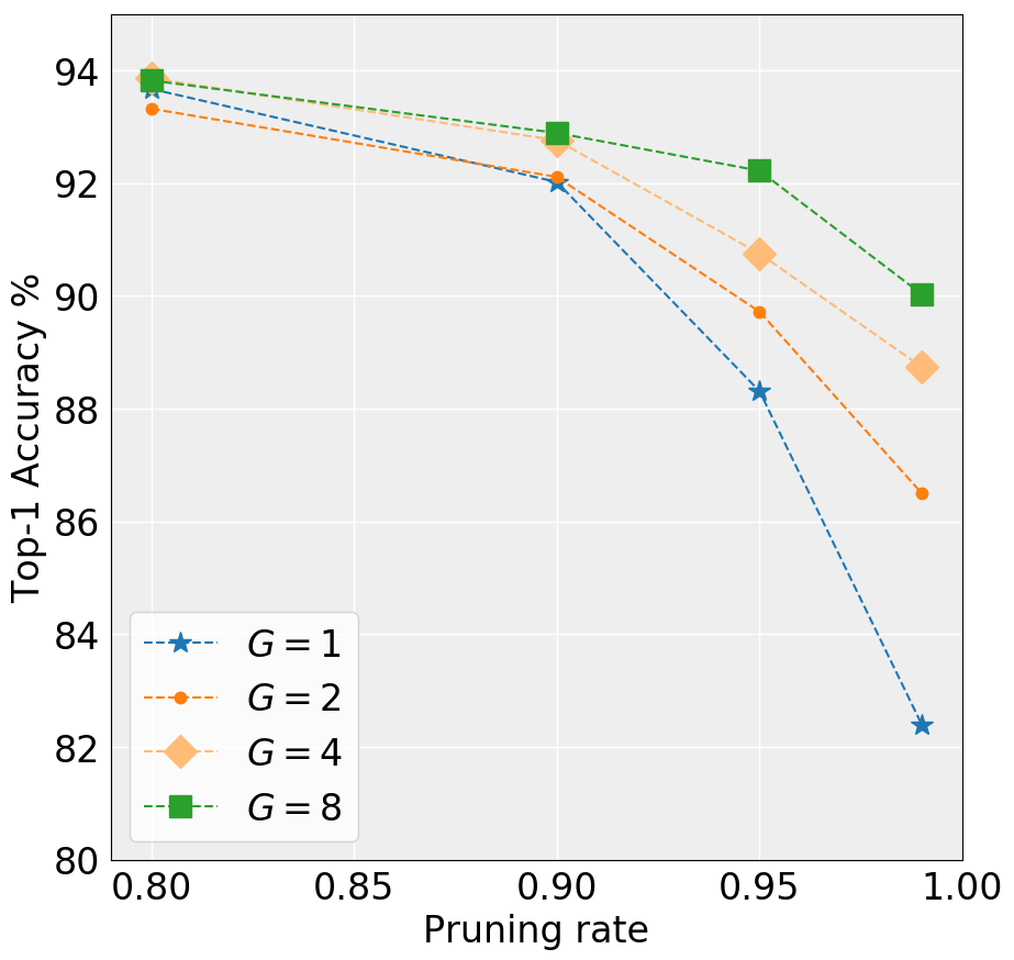
(a)

Figure 5: Importance of channel connectivity and the group extension. (left) Using more groups enables a smaller bottleneck ratio, which improves the top-end accuracy. (right) shows that increasing the minimum number of templates also reduces feature compression but at a much larger overall cost.

In the limiting case where $G=M$, the channel connectivity pattern is very similar to that of depthwise-separable convolutions since there will be a one-to-one mapping between channels in the first stage, while the second stage will be fully connected. However, there is still a significant distinction between the two - our proposed decomposition enables spatial aggregation of features in both stages.

Figure 2 demonstrates the importance of this grouped extension at high pruning rates. We find that although simply increasing the minimum number of templates in each layer does implicitly address this feature compression problem, it comes at a much larger overall cost. In general, $G$ can be tuned depending on the target pruning rate.

2.5 Computational cost and parameter efficiency.

The standard convolutional layer has the computational cost of the order of $H\cdot W\cdot K^{2}\cdot C\cdot N$, whereas the cost of the proposed decomposition is given by:

$$FLOPS= \;H\cdot W\cdot K^{2}\cdot\frac{C}{\cancel{G}}\cdot M\cdot\cancel{G}+$$ (5)

$$H\cdot W\cdot K^{2}\cdot G\cdot(N-M)$$

Where $M$ indicates the number of templates and $G$ is the number of groups. The reduction in computation ($FLOPS\downarrow$) is subsequently given by:

$$FLOPS\downarrow =\frac{HWK^{2}\cdot C\cdot M+HWK^{2}\cdot G\cdot(N-M)}{HWK^{2}\cdot C\cdot N}$$ (6)

$$={\color[rgb]{0.21875,0.390625,0.98828125}\frac{M}{N}+\frac{G}{C}}-{\color[rgb]{0.8515625,0.34375,0.27734375}\frac{GM}{CN}}$$ (7)

We prune the set of templates such that $M\ll N$ and we set $G\ll C$ to yield a reduction in FLOPs. We further improve the bottleneck problem by using $G\cdot M$ templates applied to $C/G$ channels that are efficiently implemented with grouped convolutions. Finally, we ensure cross-group information flow by increasing the number of cheap spatial transformations that are then applied cross group.

From a similar view, we can also derive the reduction in parameters, where the number of parameters for a convolutional layer is given by:

$$PARAMS=K^{2}\cdot C\cdot N$$ (8)

and our proposed decomposition has a parameter count given by:

$$PARAMS=K^{2}\cdot\frac{C}{G}\cdot M+K^{2}\cdot G\cdot(N-M)$$ (9)

Not the subtraction is because we use $M$ identity transformation, while the rest of the output features are computed using cheap spatial transformations. Using both 8 and 9, we can derive the reduction in parameters ($PARAMS\downarrow$), which ends up being identical to equation 7.

$$PARAMS\downarrow =\frac{K^{2}\cdot\frac{C}{G}\cdot M+K^{2}\cdot G\cdot(N-M)}{K^{2}\cdot C\cdot N}$$ (10)

$$={\color[rgb]{0.21875,0.390625,0.98828125}\frac{M}{GN}+\frac{G}{C}}-{\color[rgb]{0.8515625,0.34375,0.27734375}\frac{GM}{CN}}$$ (11)

When using more general and expressive spatial transformations, such as $GL(3)$ or $SO(3)$, the second stage can instead be implemented using a bilinear sampling of neighbouring spatial pixels in $\mathcal{Z}$. These transformations will be parameterised using a $2\times 3$ matrix and result in the number of floating point operations being increased to $4$ per spatial location. This increase in FLOPs and the number of parameters is often small, but it enables a significant increase in the expressiveness of transformations. However, in general, we observe that a learned scalar transformations can still yield a strong accuracy v.s. performance trade-off (see figure 2 left and table 3). We wish to highlight that in the case of these more general spatial transformations, the parameter reduction equation 11 and flop reduction equation 7 will differ.

3 Experiments

Model Method Baseline Acc. (%) Acc. (%) Acc. Drop (%) FLOPs $\downarrow$ (%) Parameters $\downarrow$ (%) VGG16 Hinge [29] 93.59 94.02 -0.43 39.07 19.95 Ours 93.26 93.92 -0.66 45.56 56.77 NSPPR [58] 93.88 93.92 -0.04 54.00 - AOFP [7] 93.38 93.84 -0.46 60.17 - DLRFC [16] 93.25 93.93 -0.68 61.23 92.86 DPFPS [44] 93.85 93.67 0.18 70.85 93.92 Ours 93.26 93.62 -0.36 61.38 81.15 ABC [30] 93.02 93.08 -0.06 73.68 88.68 HRank [32] 93.96 91.23 2.73 76.50 92.00 AOFP [7] 93.38 93.28 0.10 75.27 - Ours 93.26 92.74 0.52 80.89 95.26 NISP [55] 93.04 93.01 0.03 43.60 42.60 ResNet56 Ours 93.60 94.18 -0.58 35.91 51.64 FPGM [15] 93.59 93.49 0.10 53.00 - NSPPR [58] 93.83 93.84 -0.03 47.00 - ABC [30] 93.26 93.23 0.03 54.13 54.20 SRR-GR [51] 93.38 93.75 -0.37 53.80 - Ours 93.60 93.35 0.25 48.27 71.24 DPFPS [44] 93.81 93.20 0.61 52.86 46.84 Ours 93.60 92.81 0.79 56.36 80.05

Table 1: Comparison to other pruning methods on CIFAR10. Each model is trained using a magnitude based measure for selecting the filter templates, number of groups = 2, and with a minimum of 8 template filters per layer to avoid catastrophic pruning.

In this section we evaluate our approach on the CIFAR and ImageNet datasets. The models are compared through the number of parameters, the number of floating point operations, followed by the top-1 classification accuracy. All of these models are trained on a single NVIDIA RTX 2080Ti GPU using either stochastic gradient descent (CIFAR10) or AdamW (ImageNet-1K). We set the minimum number of templates for each layer to be 8 for CIFAR10 and 32 for ImageNet-1K. Finally, we use the number of groups in each layer to be 2 for all the main benchmark experiments

3.1 Experimental results on CIFAR-10

The CIFAR10 dataset [24] consist of 60K $32\times 32$ RGB images across 10 classes and with a 5:1 training/testing split. The chosen VGG16 [45] architecture is modified for this dataset with batch normalisation layers after each convolution block and by reducing the number of classification layers to one. During training, we augment the datasets using random horizontal flips, random $32\times 32$ crops, and random rotations. The baseline architectures are trained for 300 epochs with a step learning rate decay and we use a simple magnitude based criterion for ordering and selecting the most important filters to form the set of templates. This selection is in conjunction with a simple linear pruning schedule that spans the first 40 epochs of training. We highlight that this choice of pruning schedule is in contrast to most of the other pruning methods [59, 35], which can adopt much longer pruning stages and introduce additional layer-by-layer stopping conditions. The results are shown in table 1 and show comparable or improved performance to the much more sophisticated pruning strategies across a wide range of compression ratios.

3.2 Experimental results on ImageNet-1K

For experiments on ImageNet-1K we use the ResNet-50 architecture and the same magnitude based saliency measure described in section 3.1. In general, magnitude pruning was empirically shown to provide a more uniform pruning rate across all of the residual blocks, which is important to avoid overly compressing intermediate features. We set the minimum number of templates for each layer to be 8 and the number of groups in each layer to be 2. The model is trained for a 300 epochs with a linear learning rate decay every 25 epochs. Finally, we use MixUp and CutMix augmentations with $\alpha$ set to $0.1$ and $1.0$ respectively.

The ImageNet results are shown in table 2 and show comparable performance to state-of-the-art pruning methods without the need for extensive pruning and fine-tuning pipelines. To further demonstrate the robustness of this decomposition to the choice of templates and the effectiveness of joint template/transformation training, we propose to begin training from a randomly initialised network. In doing so, we attain comparable performance other pruning methodologies, without the need for any sophisticated pruning pipeline and stopping conditions.

Model Method Baseline Acc. (%) Acc. (%) FLOPs $\downarrow$ (%) Parameters $\downarrow$ (%) ResNet50 G-SD-B [33] 76.15 75.85 44 23 MetaPruning [34] 76.60 75.40 50 - NSPPR [58] 76.15 75.63 54 - DPFPS [44] 76.15 75.55 46 - S-COP [48] 76.15 75.26 54 52 LRF-60 [22] 76.15 75.71 56 53 DLRFC [16] 76.13 75.84 54 40 Ours 76.20 75.59 47 40

Table 2: Comparison to other pruning methods on ImageNet-1K. Our model is trained from random initialisation and with a simple magnitude based criterion. Using number of groups = 2 and with a minimum of 32 templates per layer.

3.3 Ablation experiments

Group extension.

To demonstrate the benefit of our proposed group extension, we train a VGG16 network at different pruning rates and with a varying number of groups. The results in figure 5 (left) show that at high pruning rates, whereby the layer will incur a large compression of features, increasing the number of groups will help. Although increasing the minimum number of templates per layer can also partially address this problem as shown in figure 5 (right), it would come with a much more significant computational overhead. In practice, we find that carefully selecting both the minimum number of templates and the number of groups can lead to the best performance trade-off.

Transformation family.

We explore the importance of choosing a suitable parametric family of transformations for the template filters. To do this, we first consider simple scalar multiplications of the templates, and then we consider learnable rotations. Finally, we consider the more expressive affine transformations. The results are shown in figure 3. We find that introducing more expressive transformations does improve the attainable performance, which is more significant at the higher pruning rates.

We explore the importance of selecting an appropriate parametric family of transformations for the template filters. To do this, we first consider a simple scalar multiplications applied to the templates. Subsequently, we extend our analysis to encompass learnable rotations, further expanding the range of potential transformations. Finally, to unlock the full expressive transformations, we consider the general linear group, which provide a richer and more versatile set of manipulations.

The empirical findings from our experiments are presented in the illustrative Figure 3, which serves as a visual representation of the attained results. Notably, we observe a discernible improvement in performance as we progress from simpler transformations to more expressive ones. This enhancement is particularly pronounced when operating at higher pruning rates, highlighting the significance of embracing the full spectrum of transformation possibilities.

Transformations Top-1 Accuracy Pruning Rate Scalar 90.62% 0.9 SO(3) 92.32% 0.9 GL(3) 92.33% 0.9 Scalar 92.48% 0.7 SO(3) 93.48% 0.7 GL(3) 93.57% 0.7

Table 3: Ablating the family of transformations. Increasing the expressivity of transformations has a small improvement in performance, suggesting that most of the network capacity is reserved for depthwise feature aggregation.

Visualising learned transformations.

Figure 3 provides a comparison between the original filters, the reconstructed filters, and the pruned filters. We can discern that the the reconstructed filters are significantly distinct, thus enabling highly discriminative features for the downstream task. This result is in stark contrast with conventional pruning, which simply zeroes out these pruned filters. This visualisation highlights the significance of our novel approach which not only prunes but also actively reconstructs the filters, resulting in more informative representation of the data.

Efficient Implementation.

To demonstrate that the theoretical reduction in FLOPs can translate to a real reduction in latency, we implement a simple CUDA kernel for the decomposed layer. The results are shown in figure 7, where we can see that at even moderate pruning rates there is a noticeable reduction in latency in comparison to the standard convolutional layer. We can also see that a large proportion of the latency is being spent on computing the template features, while a much smaller proportion comes from the scalar transformation of these features, which is implemented through a parallelized gather operation.

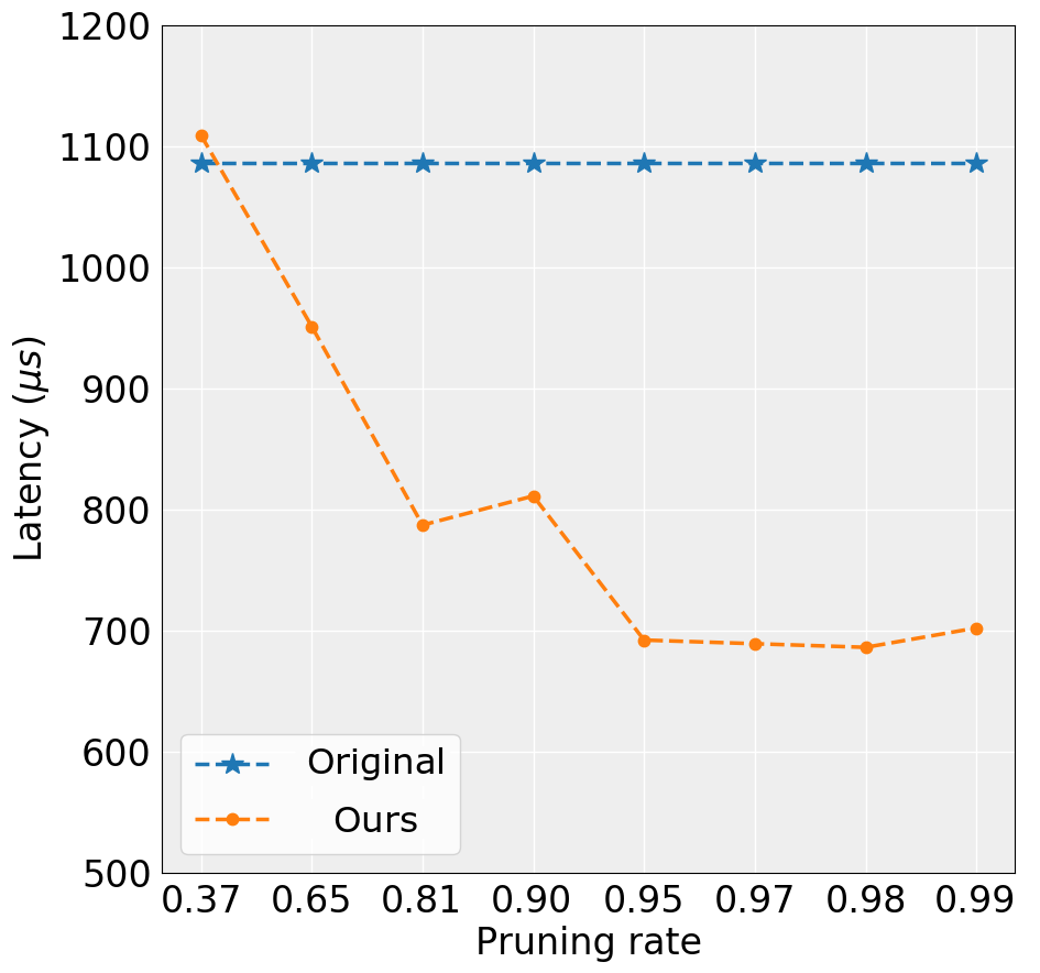
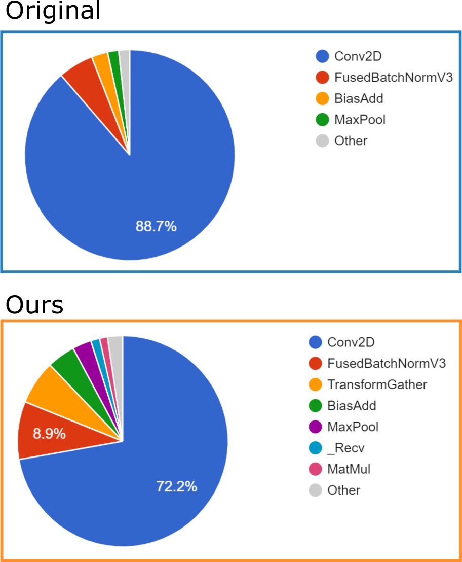
(a)

Figure 7: Latency of the proposed decomposition with an efficient implementation. (left) Compute time of an original VGG16 network with and without the decomposition at various pruning rates. (right) Cumulative contribution of each operation on the overall on-device compute time.

4 Conclusion and Future work

In this paper, we proposed the use of cheap transformations to reconstruct pruned filters. Instead of zeroing out the pruned filters, they are replaced with spatial transformations from the remaining set of non-pruned filters. These trained networks are able to achieve comparable or improved results on the image classification task across a range of datasets and architectures, despite using a simple magnitude based pruning criterion. We also introduce a grouped extension that can mitigate excessive feature compression at a minimal computational cost. Our approach applied to VGG16, ResNet34 and ResNet50 is able to significantly reduce the models size and computational cost while retaining the top recognition accuracy on CIFAR-10 and ImageNet-1K datasets.

Future research may explore potential applications in localization tasks that rely on equivariant features. Additionally, another promising direction is in data-efficient training. By incorporating hand-crafted transformations and leveraging prior knowledge of the data, it becomes possible to eliminate the necessity for the network to learn this information. Finally, we hope that this work will lead the further co-design of more weight decompositions using generalised pruning pipelines.

References

- [1] Mart Van Baalen et al. “Bayesian Bits : Unifying Quantization and Pruning”, 2020
- [2] Hong Yen Chen and Chung Yen Su “An Enhanced Hybrid MobileNet” In iCAST, 2018
- [3] Yudong Chen et al. “Improved Feature Distillation via Projector Ensemble” In NeurIPS, 2022
- [4] François Chollet “Xception: Deep Learning with Depthwise Separable Convolutions” In CVPR, 2017
- [5] Taco S. Cohen and Max Welling “Group equivariant convolutional networks” In ICML, 2016
- [6] Daniel Detone, Tomasz Malisiewicz and Andrew Rabinovich “SuperPoint: Self-supervised interest point detection and description” In ICPR, 2018
- [7] Xiaohan Ding et al. “Approximated Oracle Filter Pruning for Destructive CNN Width Optimization” In ICML, 2019
- [8] Xin Dong, Shangyu Chen and Sinno Jialin Pan “Learning to Prune Deep Neural Networks via Layer-wise Optimal Brain Surgeon” In NeurIPS, 2017
- [9] Michael H. Fox, Kyungmee Kim and David Ehrenkrantz “MobileNetV2: Inverted Residuals and Linear Bottlenecks” In CVPR, 2018
- [10] Shaopeng Guo, Yujie Wang, Quanquan Li and Junjie Yan “DMCP: Differentiable Markov Channel Pruning for Neural Networks” In CVPR, 2020
- [11] Kai Han et al. “GhostNet: More Features from Cheap Operations” In CVPR, 2019
- [12] Song Han, Huizi Mao and William J. Dally “Deep Compression: Compressing Deep Neural Networks with Pruning, Trained Quantization and Huffman Coding” In ICLR, 2015
- [13] Babak Hassibi and David G Stork “Second order derivatives for network pruning: Optimal Brain Surgeon” In NeurIPS, 1993
- [14] Kohei Hayashi, Taiki Yamaguchi, Yohei Sugawara and Shin-ichi Maeda “Einconv: Exploring Unexplored Tensor Decompositions for Convolutional Neural Networks” In NeurIPS 2019, 2019
- [15] Yang He et al. “Filter Pruning via Geometric Median for Deep Convolutional Neural Networks Acceleration” In CVPR, 2018
- [16] Zhiqiang He et al. “Filter Pruning via Feature Discrimination in Deep Neural Networks” In ECCV, 2022
- [17] Geoffrey Hinton, Oriol Vinyals and Jeff Dean “Distilling the Knowledge in a Neural Network” In NeurIPS, 2015
- [18] Frank L. Hitchcock “The Expression of a Tensor or a Polyadic as a Sum of Products” In JMP, 2015
- [19] Andrew Howard et al. “Searching for MobileNetV3” In ICCV, 2019
- [20] Hengyuan Hu, Rui Peng, Yu-Wing Tai and Chi-Keung Tang “Network Trimming: A Data-Driven Neuron Pruning Approach towards Efficient Deep Architectures” In arXiv, 2016
- [21] Max Jaderberg, Andrea Vedaldi and Andrew Zisserman “Speeding up convolutional neural networks with low rank expansions” In BMVC, 2014
- [22] Donggyu Joo, Eojindl Yi, Sunghyun Baek and Junmo Kim “Linearly Replaceable Filters for Deep Network Channel Pruning” In AAAI, 2021
- [23] Yong-Deok Kim et al. “Compression of Deep Convolutional Neural Networks for Fast and Low Power Mobile Applications” In ICLR, 2015
- [24] Alex Krizhevsky “Learning Multiple Layers of Features from Tiny Images”, 2009
- [25] Alex Krizhevsky, Ilya Sutskever and Geoffrey E Hinton “ImageNet Classification with Deep Convolutional Neural Networks” In NeurIPS, 2012
- [26] Yann Lecun “Optimal Brain Damage” In NeurIPS, 1990
- [27] Namhoon Lee, Thalaiyasingam Ajanthan and Philip H.S. Torr “SnIP: Single-shot network pruning based on connection sensitivity” In ICLR, 2019
- [28] Hao Li et al. “Pruning Filters For Efficient Convnets” In ICLR, 2017
- [29] Yawei Li et al. “Group Sparsity: The Hinge Between Filter Pruning and Decomposition for Network Compression” In CVPR, 2020
- [30] Mingbao Lin et al. “Channel Pruning via Automatic Structure Search” In IJCAI, 2020
- [31] Mingbao Lin et al. “Filter Sketch for Network Pruning” In arXiv, 2019
- [32] Mingbao Lin et al. “HRank: Filter Pruning using High-Rank Feature Map” In CVPR, 2020
- [33] Yuchen Liu, David Wentzlaff and S. Y. Kung “Rethinking Class-Discrimination Based CNN Channel Pruning” In arXiv preprint, 2020
- [34] Zechun Liu and Tim Kwang-ting Cheng “MetaPruning: Meta Learning for Automatic Neural Network Channel Pruning” In ICCV, 2019
- [35] Jian Hao Luo, Jianxin Wu and Weiyao Lin “ThiNet: A Filter Level Pruning Method for Deep Neural Network Compression” In ICCV, 2017
- [36] Roy Miles and Krystian Mikolajczyk “A closer look at the training dynamics of knowledge distillation” In arXiv preprint, 2023
- [37] Roy Miles and Krystian Mikolajczyk “Compression of descriptor models for mobile applications” In ICASSP, 2021
- [38] Roy Miles, Adrian Lopez Rodriguez and Krystian Mikolajczyk “Information Theoretic Representation Distillation” In BMVC, 2022
- [39] Roy Miles, Mehmet Kerim Yucel, Bruno Manganelli and Albert Saa-Garriga “MobileVOS: Real-Time Video Object Segmentation Contrastive Learning meets Knowledge Distillation” In CVPR, 2023
- [40] Pavlo Molchanov et al. “Importance Estimation for Neural Network Pruning” In CVPR, 2019
- [41] Qi Qian, Hao Li and Juhua Hu “Efficient Kernel Transfer in Knowledge Distillation” In arXiv, 2020
- [42] Zhuwei Qin, Fuxun Yu, Chenchen Liu and Xiang Chen “CAPTOR: A Class Adaptive Filter Pruning Framework for Convolutional Neural Networks in Mobile Applications” In ASPDAC, 2019
- [43] Adriana Romero et al. “FitNets: Hints For Thin Deep Nets” In ICLR, 2015
- [44] Xiaofeng Ruan et al. “DPFPS: Dynamic and Progressive Filter Pruning for Compressing Convolutional Neural Networks from Scratch” In AAAI, 2021
- [45] Karen Simonyan and Andrew Zisserman “Very Deep Convolutional Networks For Large-scale Image Recognition” In ICLR, 2015
- [46] Arvind Subramaniam and Avinash Sharma “N2NSkip: Learning Highly Sparse Networks using Neuron-to-Neuron Skip Connections” In BMVC, 2020
- [47] Mingxing Tan et al. “MnasNet: Platform-Aware Neural Architecture Search for Mobile” In CVPR, 2018
- [48] Yehui Tang et al. “SCOP: Scientific Control for Reliable Neural Network Pruning” In NeurIPS, 2020
- [49] Ledyard R Tucker “Some mathematical notes on three-mode factor analysis” In Psychometrika, 1966
- [50] Wenqi Wang, Brian Eriksson and Wenlin Wang “Wide Compression : Tensor Ring Nets” In CVPR, 2018
- [51] Wenxiao Wang et al. “COP: Customized deep model compression via regularized correlation-based filter-level pruning” In IJCAI, 2019
- [52] Junho Yim “A Gift from Knowledge Distillation: Fast Optimization, Network Minimization and Transfer Learning” In CVPR, 2017
- [53] Jiahui Yu and Thomas Huang “Universally Slimmable Networks and Improved Training Techniques” In ICCV, 2019
- [54] Jiahui Yu et al. “Slimmable Neural Networks” In ICLR, 2018
- [55] Ruichi Yu et al. “NISP: Pruning Networks Using Neuron Importance Score Propagation” In CVPR, 2018
- [56] Xiangyu Zhang, Xinyu Zhou and Mengxiao Lin “ShuffleNet: An Extremely Efficient Convolutional Neural Network for Mobile Devices” In CVPR, 2018
- [57] Chenglong Zhao, Bingbing Ni, Jian Zhang and Qiwei Zhao “Variational Convolutional Neural Network Pruning” In CVPR, 2019
- [58] Tao Zhuang et al. “Neuron-level Structured Pruning using Polarization Regularizer” In NeurIPS, 2022
- [59] Zhuangwei Zhuang et al. “Discrimination-aware Channel Pruning for Deep Neural Networks” In NeurIPS, 2018