Operator Shifting for Model-based Policy Evaluation

Abstract

In model-based reinforcement learning, the transition matrix and reward vector are often estimated from random samples subject to noise. Even if the estimated model is an unbiased estimate of the true underlying model, the value function computed from the estimated model is biased. We introduce an operator shifting method for reducing the error introduced by the estimated model. When the error is in the residual norm, we prove that the shifting factor is always positive and upper bounded by $1+O\left({1}/{n}\right)$, where $n$ is the number of samples used in learning each row of the transition matrix. We also propose a practical numerical algorithm for implementing the operator shifting.

90C40, 15B51

1 Introduction

Reinforcement learning (RL) has received much attention following recent successes, such as AlphaGo and AlphaZero [25, 26]. One of the fundamental problems of RL is policy evaluation [29]. When the transition dynamics are unknown, one learns the dynamics model from observed data in model-based RL. However, even if the learned model is an unbiased estimate of the true dynamics, the policy evaluation under the learned model is biased. The question of interest in this paper is whether one can increase the accuracy of the policy evaluation given an estimated dynamics model.

We consider a discounted Markov decision process (MDP) $\mathcal{M}=(\mathbb{S},\mathbb{A},P,r,\gamma)$ with discrete state space $\mathbb{S}$ and discrete action space $\mathbb{A}$. $\left\lvert\mathbb{S}\right\rvert$ and $|\mathbb{A}|$ are used to denote the size of $\mathbb{S}$ and $\mathbb{A}$, respectively. $P$ is a third-order tensor, where for each action $a\in\mathbb{A}$, $P^{a}\in\mathbb{R}^{\left\lvert\mathbb{S}\right\rvert\times\left\lvert\mathbb{S}\right\rvert}$ is the transition matrix between the states. $r$ is a second-order tensor that $r_{s,a}$ is the reward at state $s\in\mathbb{S}$ if action $a\in\mathbb{A}$ is taken. Finally, $\gamma\in(0,1)$ is the discount factor. A policy $\pi$ is a second-order tensor, where for each state $s\in\mathbb{S}$, $\pi_{s}$ represents the probability distribution over $\mathbb{A}$. At each time step $t$, one observes a state $s_{t}\in\mathbb{S}$ and takes an action $a_{t}\in\mathbb{A}$ according to the policy $\pi_{s_{t}}$. The environment returns the next state $s_{t+1}$ according to the distribution $P^{a_{t}}_{s_{t},\cdot}$ and an associated reward $r_{s_{t},a_{t}}$. The state value function $v^{\pi}\in\mathbb{R}^{\left\lvert\mathbb{S}\right\rvert}$ is the expected discounted cumulative reward if one starts from an initial state $s$ and follows a policy $\pi$, i.e., the $s$-th component is

$$v^{\pi}_{s}=\underset{\begin{subarray}{c}a_{t}\sim\pi_{s_{t}}\\ s_{t+1}\sim P^{a_{t}}_{s_{t},\cdot}\end{subarray}}{\mathbb{E}}\left[\sum_{t\geq 0}\gamma^{t}r_{s_{t},a_{t}}|s_{0}=s\right].$$

Given a policy $\pi$, the goal of policy evaluation in MDP is to solve for $v^{\pi}$. Let $b^{\pi}\in\mathbb{R}^{\left\lvert\mathbb{S}\right\rvert},P^{\pi}\in\mathbb{R}^{\left\lvert\mathbb{S}\right\rvert\times\left\lvert\mathbb{S}\right\rvert}$ be the reward vector and the transition matrix under policy $\pi$, i.e.,

$$b^{\pi}=\sum_{a}r_{sa}\pi^{a}_{s},\quad P^{\pi}=\sum_{a}P^{a}_{ss^{\prime}}\pi^{a}_{s}.$$ (1.1)

The value function $v^{\pi}$ satisfies the Bellman equation [29] $\left(I-\gamma P^{\pi}\right)v^{\pi}=b^{\pi}$. For notational simplicity, we drop the dependency on $\pi$ and write this system as

$$(I-\gamma P)v=b.$$ (1.2)

In practice, the true transition matrix $P$ and the reward vector $b$ are often inaccessible. In the model-based RL, one approximates the transition matrix $P$ and the reward vector $b$ by the empirical data $\hat{P}$ and $\hat{b}$ estimated from samples, respectively [16, 6, 28, 31, 22]. A naive approach is to solve

$$\left(I-\gamma\hat{P}\right)\hat{v}=\hat{b}.$$ (1.3)

Even if $\hat{P}$ and $\hat{b}$ are unbiased estimates for $P$ and $b$, $\hat{v}=\left(I-\gamma\hat{P}\right)^{-1}\hat{b}$ is a biased estimate for $v$, i.e., $\mathbb{E}_{\hat{P},\hat{b}}\hat{v}\neq v$.

The operator shifting idea was introduced in [10, 9] to address this issue. The paper [10] considers the noisy symmetric elliptic systems, while the follow-up paper [9] addresses the asymmetric setting under the assumption that $\hat{b}$ is isotropic, i.e., $\mathbb{E}[\hat{b}\hat{b}^{\top}]=I$. However, this isotropic condition often fails to hold in RL. In this paper, we extend the operator shifting framework to general MDPs of form (1.2). When applying this framework to the MDP setting, we add an appropriately chosen matrix $\hat{K}$ to the operator $\left(I-\gamma\hat{P}\right)^{-1}$ so that the shifted estimate $\tilde{v}=\left[\left(I-\gamma\hat{P}\right)^{-1}-\beta\hat{K}\right]\hat{b}$ is a better estimate than $\hat{v}$ in the sense that,

$$\mathbb{E}_{\hat{P},\hat{b}}\left\lVert\tilde{v}-v\right\rVert^{2}<\mathbb{E}_{\hat{P},\hat{b}}\left\lVert\hat{v}-v\right\rVert^{2}$$ (1.4)

for a certain norm $\left\lVert\cdot\right\rVert$.

Contributions.

We derive a stable shifted operator for model-based policy evaluation without assumptions on the underlying transition dynamics or reward vectors. When the approximated transition matrix $\hat{P}$ follows the multinomial distribution and $n$ samples are used to learn each row of the transition matrix $P$,

• we prove that the optimal shifting factor is always positive and upper bounded by $1+O\left(\frac{1}{n}\right)$ for any $P$ and $b$, which guarantees the stability of the shifted operator, and

• we propose a numerical algorithm to find the optimal shifting factor, which is more efficient and accurate than the bootstrapping method proposed in [10].

Related work.

Our problem is a special instance of the larger field of uncertainty quantification (UQ). In most UQ problems, one assumes that the operator (linear or non-linear) and the source term are generated from known distributions, and the task is to estimate certain quantities (such as moments, tail bounds) of the distribution of the solution. A large variety of numerical methods have been developed in UQ for this purpose in the last two decades [11, 13, 15, 33, 23, 8, 27, 17], including Monte-Carlo and quasi Monte-Carlo methods [20, 18, 4, 7, 12], stochastic collocation methods [1, 21, 34, 3], stochastic Galerkin methods [2, 35, 5, 19], and etc. The problem that we face is somewhat different: since the true $P$ and $b$ are unknown, one does not know the distributions of the empirical data $\hat{P}$ or $\hat{b}$. As a result, the solution relies more on statistical techniques such as shrinkage [14] rather than the traditional UQ techniques.

Contents.

Section 2 derives the oracle estimators and proves their lower and upper bounds. Section 3 proposes a practical estimator and demonstrates its performance with a few numerical examples. Section 4 contains all the proofs of the main results.

2 Operator Shifting for Policy Evaluation

2.1 Problem setup.

As mentioned above, $P$ and $b$ are the unknown underlying transition matrix and reward vector, while $\hat{P}$ and $\hat{b}$ are unbiased estimates for $P$ and $b$, respectively. For notational convenience, we introduce $A$ and $\hat{A}$

$$A=\left(I-\gamma P\right),\quad\hat{A}=\left(I-\gamma\hat{P}\right).$$ (2.1)

Since the transition dynamics is not symmetric in general, both $P$ and $A$ are non-symmetric. The norm of interest is a slightly generalized version of the residual norm

$$\left\lVert x\right\rVert^{2}_{M}=x^{\top}A^{\top}MAx,$$ (2.2)

where $M$ is a symmetric positive definite matrix. This paper mainly discusses two cases: (1) $M=I$, which means $\left\lVert\cdot\right\rVert_{M}$ is the usual residual norm, and (2) $M=A^{-\top}A^{-1}$, which means $\left\lVert\cdot\right\rVert_{M}$ is the $l_{2}$ norm.

In this paper, we choose the shifting matrix $\hat{K}=\hat{A}^{-1}$, which implies that the shifted estimate is $\left(1-\beta\right)\hat{A}^{-1}\hat{b}$. By using $\varepsilon=\left(1-\beta\right)$ instead as the shifting parameter, one can write the above estimate as $\tilde{v}_{\varepsilon}\equiv\varepsilon\hat{A}^{-1}\hat{b}$, and the objective is to minimize the following mean square error over $\varepsilon$,

$$\mathrm{MSE}(\varepsilon)\equiv\mathbb{E}_{\hat{P},\hat{b}}\left\lVert v-\tilde{v}_{\varepsilon}\right\rVert_{M}^{2}.$$ (2.3)

The minimizer $\varepsilon^{*}$ to (2.3) is referred as the optimal shifting factor.

Since (2.3) is a quadratic minimization, one can explicitly write out the optimal shifting factor $\varepsilon^{*}$:

$$\varepsilon^{*}=\frac{\mathbb{E}_{\hat{P},\hat{b}}\left[b^{\top}MA\hat{v}\right]}{\mathbb{E}_{\hat{P},\hat{b}}\left[\hat{v}^{\top}A^{\top}MA\hat{v}\right]},\quad\text{where}\;\hat{v}=\hat{A}^{-1}\hat{b}.$$ (2.4)

The oracle estimate (2.4) is not easy to work with as it depends on the unknown matrix $A$. Our immediate goal is to derive a closed-form approximation of $\varepsilon^{*}$, which is accurate and allows for efficient implementation. To achieve this, we introduce a second-order approximation $\varepsilon^{\circ}$ to $\varepsilon^{*}$. We show that $\varepsilon^{\circ}$ takes a simple closed-form without approximating any expectations under the following mild assumption:

• Assumption 1: The $i$-th row $\hat{p}^{\top}_{i}$ of $\hat{P}$ is an random vector $\frac{1}{n_{i}}X_{i}$, where $n_{i}$ is the number of samples for state $i$ and $X_{i}$ follows the multinomial distribution with $\mathbb{E}[X_{i}]=n_{i}p^{\top}_{i}$. Moreover, $X_{i}$ is independent from $X_{j}$ whenever $i\not=j$. The $i$-th entry of $\hat{b}$ is an average of observed reward at state $i$.

The part of Assumption 1 on the estimation of $P$ is equivalent to that $\hat{p}^{\top}_{i}$ follows the normalized multinomial distribution, which holds when a tabular maximum likelihood model [28] is used to estimate the transition dynamics $P$. That is, one generates sufficiently many transitions according to $P$ and lets $\hat{P}_{ii^{\prime}}=n_{ii^{\prime}}/n_{i},$ where $n_{ii^{\prime}}$ denotes the number of transitions observed from $i$ to $i^{\prime}$, and $n_{i}=\sum_{i^{\prime}}n_{ii^{\prime}}$.

Throughout this paper, we assume for simplicity that the number of samples $n_{i}$ of each state is the same, i.e., for any $i\in\mathbb{S}$, $n_{i}\equiv n$. The sample size $n$ plays an important role in determining the magnitude of the operator shifting factor $\varepsilon^{*}$ and the performance of the operator shifting algorithm. If the value of $n_{i}$ depends on $i\in\mathbb{S}$, all the theoretical results still hold with slight modification (see Remark 2.3 for details).

2.2 Second-order approximation for $\varepsilon^{*}$.

To simplify the discussion, we introduce $\hat{Z}$ and $\hat{Y}$

$$\hat{Z}=A-\hat{A}=\gamma\left(P-\hat{P}\right),\quad\hat{Y}=\hat{Z}A^{-1}=\left(A-\hat{A}\right)A^{-1},$$ (2.5)

where $A$ and $\hat{A}$ are defined in (2.1). Some basic algebraic manipulations lead to the following lemma.

Lemma 2.1.

When $\displaystyle\mathbb{E}\left[\hat{b}\right]=b$, the optimal shifting factor $\varepsilon^{*}$ defined in (2.4) has the form

$$\varepsilon^{*}=\frac{\mathbb{E}_{\hat{P}}\left[b^{\top}M\left(I-\hat{Y}\right)^{-1}b\right]}{\mathbb{E}_{\hat{P}}\left[\mathrm{tr}\left(\left(\mathrm{cov}\left[\hat{b}\right]+b^{\top}b\right)\left(I-\hat{Y}\right)^{-\top}M\left(I-\hat{Y}\right)^{-1}\right)\right]},$$ (2.6)

where $\hat{Y}$ is defined in (2.5). Moreover, if the values of the reward at state $s$ and $s^{\prime}$ (i.e. $\hat{b}_{s}$ and $\hat{b}_{s^{\prime}}$) are uncorrelated, the matrix $\mathrm{cov}[\hat{b}]$ is diagonal.

Next, we approximate the value of $\varepsilon^{*}$ using a Neumann expansion of the matrix $\left(I-\hat{Y}\right)^{-1}$

$$\left(I-\hat{Y}\right)^{-1}=I+\hat{Y}+\hat{Y}^{2}+O\left(\frac{\rho(\hat{Y})^{3}}{1-\rho(\hat{Y})}\right),$$ (2.7)

when the spectral radius $\rho(\hat{Y})<1$. In fact, a modest requirement on $n$ guarantees $\rho(\hat{Y})<1$ with high probability, as shown in Appendix E. The denominator term in (2.6) admits the approximation

$$\left(I-\hat{Y}\right)^{-\top}M\left(I-\hat{Y}\right)^{-1}\approx M+M\left(\hat{Y}+\hat{Y}^{2}\right)+(\hat{Y}^{\top}+(\hat{Y}^{\top})^{2})M+\hat{Y}^{\top}M\hat{Y}.$$ (2.8)

Assumption 1 implies $\mathbb{E}\left[\hat{Y}\right]=\mathbb{E}\left[\hat{Y}^{\top}\right]=0$ as a simple consequence of $\hat{P}$ being an unbiased estimator. Therefore, after taking an expectation, the first order terms of $\hat{Y}$ in (2.7) and (2.8) disappear.

We can further approximate the shifting factor $\varepsilon^{*}$ by expanding $\left(I-\hat{Y}\right)^{-1}$ in the numerator and denominator of (2.6) up to the second order in $\hat{Y}$. When Assumption 1 holds and $\rho(\hat{Y})<1$, the approximated optimal shifting factor $\varepsilon^{*}$ defined in (2.4) has a second-order approximation

$$\varepsilon^{*}\approx\varepsilon^{\circ}\equiv\frac{\mathbb{E}_{\hat{P}}\left[b^{\top}(M+\frac{M\hat{Y}^{2}+(\hat{Y}^{\top})^{2}M}{2})b\right]}{\mathbb{E}_{\hat{P}}\left[\mathrm{tr}\left(\left(\mathrm{cov}\left[\hat{b}\right]+b^{\top}b\right)(M+\hat{Y}^{\top}M\hat{Y}+M\hat{Y}^{2}+(\hat{Y}^{\top})^{2}M)\right)\right]}.$$ (2.9)

The derivation of (2.9) is deferred to Section 4.2.

Under Assumption 1, this second-order approximation can be written in a form without explicit expectation. This expectation-free form depends on the transition matrix $P$, the expected reward $b$, and the reward covariance $\mathrm{cov}\left[\hat{b}\right]$. Let $\hat{p}_{i}$ be random vectors corresponding to the i-th row of $\hat{P}$ and $p_{i}=\mathbb{E}\left[\hat{p}_{i}\right]$, i.e., $\{\hat{p}_{i}\}_{i=1}^{\left\lvert\mathbb{S}\right\rvert}$ and $\{p_{i}\}_{i=1}^{\left\lvert\mathbb{S}\right\rvert}$ are the row vectors of $\hat{P}$ and $P$, respectively:

$$\hat{P}=\begin{bmatrix}\hat{p}_{1}^{\top}\\ \dots\\ \hat{p}_{\left\lvert\mathbb{S}\right\rvert}^{\top}\end{bmatrix},\quad P=\begin{bmatrix}p_{1}^{\top}\\ \dots\\ p_{\left\lvert\mathbb{S}\right\rvert}^{\top}\end{bmatrix}.$$ (2.10)

Theorem 2.2.

The second-order approximation $\varepsilon^{\circ}$ in (2.9) admits the expectation-free form

$$\varepsilon^{\circ}=\theta(b,P)\equiv\frac{b^{\top}(M+H/2)b}{b^{\top}(M+G+H)b+\mathrm{tr}\left(\mathrm{cov}\left[\hat{b}\right](M+G+H)\right)},$$ (2.11)

where

$$\begin{cases}B_{i}=\frac{1}{n}\left(\diag{p_{i}}-p_{i}p_{i}^{\top}\right);\\ G=\mathbb{E}_{\hat{P}}\left[\hat{Y}^{\top}M\hat{Y}\right]=\gamma^{2}A^{-\top}\left(\sum_{i=1}^{\left\lvert\mathbb{S}\right\rvert}\left[M\right]_{ii}B_{i}\right)A^{-1};\\ \begin{aligned} H&=\mathbb{E}_{\hat{P}}\left[(\hat{Y}^{\top})^{2}M+M\hat{Y}^{2}\right]\\ &=\gamma^{2}\left[\sum_{i=1}^{\left\lvert\mathbb{S}\right\rvert}A^{-\top}B_{i}A^{-1}\mathrm{diag}\left(e_{i}\right)\right]M+\gamma^{2}M\left[\sum_{i=1}^{\left\lvert\mathbb{S}\right\rvert}\mathrm{diag}\left(e_{i}\right)A^{-\top}B_{i}A^{-1}\right]\end{aligned}.\end{cases}$$ (2.12)

Here $\mathrm{diag}(e_{i})\in\mathbb{R}^{\left\lvert\mathbb{S}\right\rvert\times\left\lvert\mathbb{S}\right\rvert}$ is a matrix with elements $0$ except for $1$ on the $(i,i)$-th entry, $p_{i}$ are row vectors of $P$ as defined in (2.10), and the matrices $A$ and $\hat{Y}$ depend on $P$.

The proof of the above theorem is given in Section 4.2.

Remark 2.3.

Theorem 2.2 still holds under conditions weaker than Assumption 1. Assuming the rows of $\hat{P}$ and entries for $\hat{b}$ are independent unbiased estimators, then the second-order approximation in (2.9) is still valid. Moreover, the expectation-free form in (2.11) holds when one replaces the definition of $B_{i}$ in (2.12) by $B_{i}=\mathrm{cov}\left[\hat{p}_{i}\right]$. This slightly more general statement is presented in Lemma 4.2, from which Theorem 2.2 is derived as a special case. In particular, if the state $i$ receives $n_{i}$ samples, then (2.11) will still hold with $B_{i}$ in (2.12) replaced by $\frac{1}{n_{i}}\left(\diag{p_{i}}-p_{i}p_{i}^{\top}\right)$.

Theorem 2.2 also proves that the choice of $\varepsilon^{\circ}$ is asymptotically as powerful as $\varepsilon^{*}$ with $n\to\infty$. For $\mathrm{MSE}(\varepsilon)$ defined in (2.3), the following estimation holds, with the proof deferred to Section 4.3.

Lemma 2.4.

The MSE in (2.3) can be approximated by

$$\mathrm{MSE}(\varepsilon)=\left(1-\varepsilon\right)^{2}\left\lVert b\right\rVert_{M}^{2}+(g+h+t)\varepsilon^{2}-h\varepsilon+O\left(n^{-\frac{3}{2}}\right),$$ (2.13)

where $g=b^{\top}Gb,h=b^{\top}Hb,t=\mathrm{tr}\left(\mathrm{cov}\left[\hat{b}\right]\left(M+G+H\right)\right)$ with all symbols defined in Theorem 2.2. In addition,

$$\varepsilon^{*}-\varepsilon^{\circ}=O\left(n^{-\frac{3}{2}}\right).$$ (2.14)

The relative error reduction factor $\eta\equiv\frac{\mathrm{MSE}(1)-\mathrm{MSE}(\varepsilon^{\circ})}{\mathrm{MSE}(1)}$, with MSE representing the mean square error defined in (2.3), is a useful measure for improvements. Below is a corollary of Lemma 2.4 regarding $\eta$.

Corollary 2.5.

Define relative error reduction factor as $\eta\equiv\frac{\mathrm{MSE}(1)-\mathrm{MSE}(\varepsilon^{\circ})}{\mathrm{MSE}(1)}$. For $n$ sufficiently large, $\eta$ is positive, and decays as follows

$$\eta=O\left(1/n\right),$$ (2.15)

where MSE is defined in (2.3).

The proof is given in Section 4.3. The numerical results also verify the relationship in the above Corollary.

2.3 Lower and upper bounds for $\varepsilon^{\circ}$.

In this section, we aim to provide bounds to show that $\varepsilon^{\circ}$ will approximately fall in the $(0,1)$ range. Throughout this subsection, we conduct the analysis in the residual norm, which is the case with $M=I$. We present an upper bound and a lower bound for $\varepsilon^{\circ}$ in Theorem 2.6. The relevant parameters are $\left\lvert\mathbb{S}\right\rvert$, $n$ and $\gamma$, which are the number of state, the number of samples per state and the discount factor, respectively.

Theorem 2.6.

Let $p_{M}=\max P_{i,j}$ and $b_{M}=\max_{i}|b_{i}|$. If $\frac{p_{M}}{n}\frac{\gamma^{2}}{\left(1-\gamma\right)^{2}}\left(\frac{\left(1-\gamma\right)}{\gamma}+\frac{\sqrt{\left\lvert\mathbb{S}\right\rvert}b_{M}}{\left\lVert b\right\rVert_{2}}\right)^{2}\leq\frac{1}{2}$, then $\varepsilon^{\circ}$ is bounded by

$$0<\varepsilon^{\circ}\leq 1+\frac{p_{M}}{n}\frac{\gamma^{2}}{\left(1-\gamma\right)^{2}}\left(\left(1-\gamma\right)+\gamma\frac{\sqrt{\left\lvert\mathbb{S}\right\rvert}b_{M}}{\left\lVert b\right\rVert_{2}}\right)^{2}.$$

The bound comes from technique using the spectral structure of the covariance matrix of a multinomial distribution and a tight bound for $(I-\gamma P)^{-1}b$. We defer the proof to Section 4.

We now discuss the implication of Theorem 2.6. The reward vector $b$ is spread if $\frac{\max_{i}|b_{i}|}{\left\lVert b\right\rVert_{2}}\sim O\left(\left\lvert\mathbb{S}\right\rvert^{-1/2}\right)$. Similarly, the transition matrix $P$ is spread if $\max P_{ij}\sim o\left(\left\lvert\mathbb{S}\right\rvert^{-1/2}\right)$. If both $b$ and $P$ are spread, it follows that $\epsilon^{\circ}-1$ is upper bounded by a term in $O(n^{-1}\left\lvert\mathbb{S}\right\rvert^{-1/2})$.

3 Practical algorithm

3.1 Algorithm.

In practice, we do not have direct access to $P$ or $b$. Therefore, the second-order estimate $\varepsilon^{\circ}$ derived in (2.11) is an oracle estimator. One can address this issue by bootstrapping the distribution of $\hat{P}$. More specifically, let $P$ be a transition matrix and denote $\mathcal{M}_{n}(P)$ as the normalized multinomial distribution that the estimated transition matrix $\hat{P}$ follows according to Assumption 1. Since one only has access to a single observation $\hat{P}$, $\mathcal{M}_{n}(P)$ is approximated by $\mathcal{M}_{n}(\hat{P})$ in the numerical implementation. In the usual bootstrapping procedure, one needs to simulate i.i.d. samples $\{\tilde{P}_{(j)}\}_{j=1}^{l}\sim\mathcal{M}_{n}(\hat{P})$. By setting $\tilde{Y}_{(j)}=\gamma(\tilde{P}_{(j)}-\hat{P})\hat{A}^{-1}$ and following the form in Theorem 2.2, one can approximate $\varepsilon^{\circ}$ in (2.9) by replacing the expectation with an empirical mean:

$$\varepsilon^{\circ}\approx\frac{\hat{b}^{\top}(M+\tilde{H}/2)\hat{b}}{\hat{b}^{\top}\left(M+\tilde{G}+\tilde{H}\right)\hat{b}+\mathrm{tr}\left(\tilde{\Sigma}\left(M+\tilde{G}+\tilde{H}\right)\right)},$$ (3.1)

with

$$\begin{cases}\tilde{G}=\frac{1}{l}\sum_{j=1}^{l}\tilde{Y}_{(j)}^{\top}M\tilde{Y}_{(j)}\approx\mathbb{E}_{\hat{P}}\left[\hat{Y}^{\top}M\hat{Y}\right]=G;\\ \tilde{H}=\frac{1}{l}\sum_{j=1}^{l}M\tilde{Y}_{(j)}^{2}+\left(\tilde{Y}_{(j)}^{\top}\right)^{2}M\approx\mathbb{E}_{\hat{P}}\left[M\hat{Y}^{2}+(\hat{Y}^{\top})^{2}M\right]=H;\\ \tilde{\Sigma}\approx\mathrm{cov}\left[\hat{b}\right].\end{cases}$$ (3.2)

However, there is a major drawback to this scheme. In addition to the error caused by the difference between $\mathcal{M}_{n}(\hat{P})$ and $\mathcal{M}_{n}({P})$, the scheme introduces additional errors due to the empirical mean in place of the expectation. The empirical mean errors $\tilde{G}-G$ and $\tilde{H}-H$ are of order $O\left(l^{-1/2}\right)$. In addition, the procedure in (3.1) has a computational cost of order $O\left(l\left\lvert\mathbb{S}\right\rvert^{3}\right)$.

Plug-in estimate.

Luckily in our case, Assumption 1 (i.e., $\hat{P}$ follows the normalized multinomial distribution) allows for a direct formula for $\varepsilon^{\circ}$, which automatically removes the error in the empirical mean. We can simply set

$$\tilde{\varepsilon}^{\circ}:=\theta(\hat{b},\hat{P}),$$ (3.3)

where $\theta(b,P)$ is defined in Theorem 2.2. The complete numerical algorithm is presented in Algorithm 1. The right-hand side of (3.1) converges to $\theta(\hat{b},\hat{P})$ as $l\rightarrow\infty$. In addition, the computational cost is reduced from $O\left(l\left\lvert\mathbb{S}\right\rvert^{3}\right)$ to $O\left(\left\lvert\mathbb{S}\right\rvert^{3}\right)$. This complete removal of empirical mean error is what sets the multinomial MDP case apart from general operator shifting. Moreover, since both $\varepsilon^{\circ}$ in (2.11) and $\tilde{\varepsilon}^{\circ}$ in (3.3) share the same functional form, the lower and upper bounds in Section 2.3 automatically apply to both $\varepsilon^{\circ}$ and $\tilde{\varepsilon}^{\circ}$. In all the following numerical examples, we use the approximated factor $\tilde{\varepsilon}^{\circ}$, which does not rely on oracle access.

Algorithm 1 Operator Shifting for estimating MDP (Multinomial)

Outputs the bootstrapped $\tilde{\varepsilon}^{\circ}=\theta(\hat{b},\hat{P})$. The function can also output the true value by $\varepsilon^{\circ}=\theta(b,P)$ if one has oracle access to $P,b$.

1:$\hat{P}$: Estimated transition matrix

2:$\hat{b}$: Estimated expected reward

3:$n$: Sample data size per state

4:$\tilde{\Sigma}$: Estimated covariance matrix of $\hat{b}$

5:$\gamma$: Discount factor

6:$M$: The chosen norm matrix

7:

8:function $\theta$($\hat{P},\hat{b}$)

9:     $\hat{C},\hat{D}$ $\leftarrow$ $\mathrm{zeros}(\left\lvert\mathbb{S}\right\rvert)$ $\triangleright$ $\mathrm{zeros}(n)$: A zero matrix of size $n$

10:     for $i\leftarrow 1\textrm{ to }\left\lvert\mathbb{S}\right\rvert$ do

11:         $\hat{p}_{i}$ $\leftarrow$ $\hat{P}^{\top}e_{i}$ $\triangleright$ Get the $i$-th row of $\hat{P}$

12:         $\hat{B}_{i}$ $\leftarrow$ $\frac{1}{n}\left(\hat{p}_{i}\hat{p}_{i}^{\top}-\mathrm{diag}(\hat{p}_{i})\right)$ $\triangleright$ Estimate covariance

13:         $\hat{C}$ $\leftarrow$ $\hat{C}+\hat{B}_{i}\hat{A}^{-1}\mathrm{diag}\left(e_{i}\right)$

14:         $\hat{D}$ $\leftarrow$ $\hat{D}+[M]_{ii}\hat{B}_{i}$

15:     end for

16:     $\hat{C}$ $\leftarrow$ $\gamma^{2}\hat{A}^{-\top}\hat{C}$ $\triangleright$ Approximate $\mathbb{E}\left[(\hat{Y}^{\top})^{2}\right]$

17:     $\hat{G}$ $\leftarrow$ $\gamma^{2}\hat{A}^{-\top}\hat{D}\hat{A}^{-1}$ $\triangleright$ Approximate $\mathbb{E}\left[\hat{Y}^{\top}M\hat{Y}\right]$

18:     $\hat{H}$ $\leftarrow$ $\hat{C}M+M\hat{C}^{\top}$ $\triangleright$ Approximate $\mathbb{E}\left[(\hat{Y}^{\top})^{2}M+M\hat{Y}^{2}\right]$

19:     $\tilde{\varepsilon}^{\circ}$ $\leftarrow$ $\frac{\hat{b}^{\top}\left(M+\hat{H}/2\right)\hat{b}}{\hat{b}^{\top}\left(M+\hat{G}+\hat{H}\right)\hat{b}+\mathrm{tr}\left(\tilde{\Sigma}\left(M+\hat{G}+\hat{H}\right)\right)}$

20:     return $\tilde{\varepsilon}^{\circ}$

21:end function

3.2 Numerical examples.

Policy evaluation of an MDP over a circle.

We first consider an MDP over a discrete state space $\mathbb{S}=\{k\}_{k=0}^{N-1}$ with $N=64$ and $\gamma=0.9$. The transition dynamics are given as below,

$$s_{t+1}\leftarrow s_{t}+\left(1+Z_{t}\right)a_{t}\mod{N},$$

$$r_{s_{t},a_{t}}={\sin\left(\frac{2\pi s_{t}}{N}\right)}+a_{t}{\cos\left(\frac{2\pi s_{t}}{N}\right)}/10+X_{t},$$

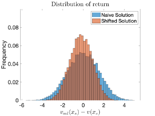
where $a_{t}\in\{\pm 1\}$ is drawn from a policy $\pi(a_{t}|s_{t})=\frac{1}{2}+\frac{1}{5}a_{t}\sin\left(\frac{2\pi s_{t}}{N}\right)$, and $X_{t}\sim N(0,\delta)$ with $\delta\in\{0,0.1,0.2\}$. When $\delta=0$, the reward is deterministic. Here $Z_{t}$ is a random integer taking values in the set $\{-\sigma,\ldots,\sigma\}$ with equal probability, where $\sigma\in\{1,2,4\}$. A larger $\sigma$ means each state could transit to more neighboring states under one step. Figure 1 illustrates the distribution of the estimated $v(x_{s})$ for $x_{s}:=0$, see caption for implementation detail. One can see that the shifted value is more concentrated around the ground truth value than the naive solution.

Figure 1: 1D circle example. Histogram of $v_{sol}(x_{s})-v(x_{s})$, where $v(x_{s})$ denotes the true return at $x_{s}$, and $v_{sol}(x_{s})$ denotes the estimated return from either the naive solution or the operator shifting solution. The shifted solution is more concentrated around the ground truth. The histogram is obtained via $20,000$ simulations, and we set $n=8$, $\delta=0.2$, and $\sigma=4$.

(a) Residual norm

(b) $l_{2}$ norm

Figure 2: 1D circle example. Error reduction as a function of $n$ for the residual norm (left) and the $l_{2}$ norm (right). The $y$-axis is the error reduction rate in MSE, relative to the error of the naive solution. The error reduction rate is inversely proportional to $n$ across different choices of $\sigma$ and $\delta$. For the residual norm case, the error reduction is heavily influenced by the choice of parameters, where a larger $\sigma$ or $\delta$ implies a larger reduction in error.

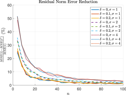
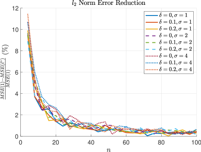
One can also bootstrap to reduce the $l_{2}$ error. Specifically, the $l_{2}$ error refers to the case when $M=A^{-\top}A^{-1}$ in the norm $\left\lVert\cdot\right\rVert_{M}$ defined in (2.2). Despite a lack of access to $A$, one can use $M=\hat{A}^{-\top}\hat{A}^{-1}$ for $l_{2}$ error minimization, which works well empirically. The error reduction trend remains the same (see Figure 2 for details). Overall, the error reduction for $l_{2}$ norm is less significant than the residual norm, though it is still significant for small $n$.

In the following examples, we focus on the results for the residual norm.

MDPs generated by random graphs.

To test the robustness of Algorithm 1, here we apply the operator shifting method to different underlying transition matrices. For consistency, we set $\left\lvert\mathbb{S}\right\rvert=64$.

As discussed in the 1D circle case, the randomness in $\hat{b}$ usually boosts the performance of the operator shifting method. Here we take out the randomness in the reward and instead let $\hat{b}$ be deterministic, i.e., $\hat{b}=b$ and $\mathrm{cov}[\hat{b}]=0$. To test different $b$, we assume that $b$ is randomly generated according to $\mathcal{N}(0,I)$. The transition matrix $P$ corresponds to the random walk on a directed random graph $G=(V,E,w)$, where $V=\mathbb{S}$ is the vertex set, $E$ is the edge set, and the edge weight is $w:E\rightarrow\mathbb{R}_{\geq 0}$.

Two types of random graphs are considered. In the first dense case, the graph $G$ is considered to be fully connected, and the weight $w(e)$ on each edge $e$ is an i.i.d. random variable following $w(e)\sim\mathcal{U}(0,1)$. In the second sparse case, a sparse graph is considered. In order to generate a random sparse graph, one initializes with a graph containing an empty edge set,

$$G\leftarrow G_{0}:=(V=\mathbb{S},E=\varnothing).$$

For each vertex $v\in V$, two vertices $v_{1},v_{2}$ are randomly selected from the set $\mathbb{S}\setminus\{v\}$ that excludes $v$ itself with equal probability, and then

$$E\leftarrow E\cup\{(v_{1},v),(v,v_{2})\}.$$

After enumerating over all vertices, one then assigns a weight of one to all existing edges in $G$. This construction ensures that none of the vertices is a well or sink node, that is, each vertex has at least one indegree and one outdegree, but the transition matrix is still quite sparse.

(a) Random dense MDP

(b) Random sparse MDP

Figure 3: Random directed graphs. Error reduction as a function of sample size $n$. Left: the random dense graph. Right: the random sparse graph.

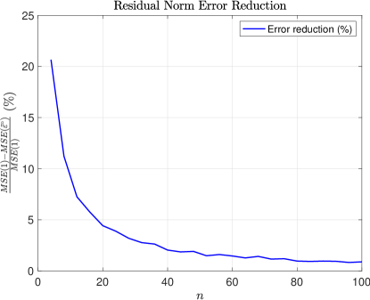
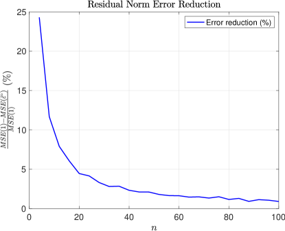
Figure 3 shows that the same MSE reduction pattern holds in the random directed graph cases. The operator shifting solution still consistently outperforms the naive solution.

Policy evaluation of an MDP over a torus.

We now consider an MDP with a discrete state space $\mathbb{S}=\{s_{ij}=(i,j)\}_{i,j=0}^{N-1}$ with $N=8$ and $\gamma=0.9$. Note that the size of the state space $|\mathbb{S}|$ is still $64$. Let $(s)_{k}$ stand for the first or second entry of the vector $s$ with $k=1$ or $2$. The transition dynamics and reward are given by

$$s_{t+1}\leftarrow s_{t}+(1+Z_{t})a_{t}\mod N,$$

$$r_{s_{t},a_{t}}\leftarrow 2+\sin\left(\frac{2\pi(s_{t})_{1}}{N}\right)+\cos\left(\frac{2\pi(s_{t})_{2}}{N}\right)+X_{t},$$

where $a_{t}\in\mathbb{A}=\{(\pm 1,0),(0,\pm 1)\}$, $X_{t}\sim N(0,\delta)$ with $\delta\in\{0,0.1,0.2\}$. Here $Z_{t}$ is a random integer taking values in the set $\{-\sigma,\ldots,\sigma\}$ with equal probability, where $\sigma\in\{1,2,4\}$. We use the policy

$$\pi(a_{t}=(a_{1},a_{2})|s_{t})=\frac{1}{4}+\frac{1}{20}\left(a_{1}\cos\left(\frac{2\pi(s_{t})_{1}}{N}\right)+a_{2}\sin\left(\frac{2\pi(s_{t})_{2}}{N}\right)\right).$$ (3.4)

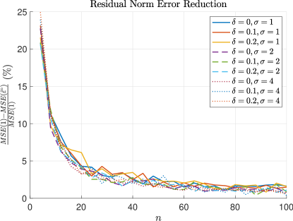
Figure 4 summarizes the performance and exhibits a similar error reduction trend. Contrary to the role of the parameters in the 1D circle case, different choices of $\sigma$ and $\delta$ do not change the performance of the operator shifting method.

Figure 4: 2D torus example. Error reduction as a function of sample size $n$.

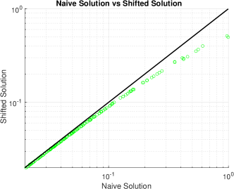
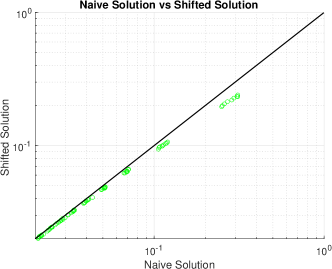
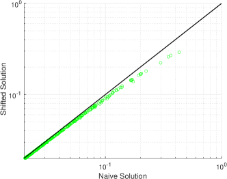
Summary of numerical experiments.

Figure 5 plots the normalized MSE of the naive solution against the operator shifting solution. In the torus and circle cases, the data points are obtained by varying the sample size $n$, the reward variance $\delta$, and the transition parameter $\sigma$. In the randomly generated MDP case, the data points are obtained by sampling random MDPs and varying the value of the sample size $n$. The vast majority of the data points are below the diagonal line, suggesting that operator shifting consistently reduces the MSE.

As a further remark, the numerical result shows that the bounds in Theorem 2.6 for $\varepsilon^{\circ}$ is quite pessimistic. In practice, $\varepsilon^{\circ}$ almost always falls in the $(0,1)$ range, even for small $n$.

(a) 1D circle

(b) 2D Torus

(c) Random dense MDP

(d) Random sparse MDP

Figure 5: The normalized MSE of the operator shifting solution is plotted against that of the naive solution. All data points are below or close to the diagonal, showing that the operator shifting solution outperforms the naive solution in all data points collected.

4 Proofs

4.1 Proof of Lemma 2.1.

Proof 4.1.

From (2.5), $\left(I-\hat{Y}\right)A\hat{v}=\left(\hat{A}A^{-1}\right)A\hat{v}=\hat{A}\hat{v}=\hat{b}$ and

$$A\hat{v}=\left(I-\hat{Y}\right)^{-1}\hat{b}.$$

Hence (2.4) can be written as

$$\varepsilon^{*} =\frac{\mathbb{E}_{\hat{P},\hat{b}}\left[b^{\top}M\left(I-\hat{Y}\right)^{-1}\hat{b}\right]}{\mathbb{E}_{\hat{P},\hat{b}}\left[\hat{b}^{\top}\left(I-\hat{Y}\right)^{-\top}M\left(I-\hat{Y}\right)^{-1}\hat{b}\right]}.$$

From Assumption 1, $\mathbb{E}[\hat{b}]=b$. Moreover, it follows from Assumption 1 that $\hat{P}$ is independent to $\hat{b}$. Hence one can write the numerator as

$$\mathbb{E}_{\hat{P},\hat{b}}\left[b^{\top}M\left(I-\hat{Y}\right)^{-1}\hat{b}\right]=\mathbb{E}_{\hat{P}}\left[b^{\top}M\left(I-\hat{Y}\right)^{-1}b\right],$$

and the denominator as

$$\mathbb{E}_{\hat{P},\hat{b}}\left[\hat{b}^{\top}\left(I-\hat{Y}\right)^{-\top}M\left(I-\hat{Y}\right)^{-1}\hat{b}\right]$$

$$= \mathbb{E}_{\hat{P}}\left[b^{\top}\left(I-\hat{Y}\right)^{-\top}M\left(I-\hat{Y}\right)^{-1}b\right]+\mathbb{E}_{\hat{P},\hat{b}}\left[(b-\hat{b})^{\top}\left(I-\hat{Y}\right)^{-\top}M\left(I-\hat{Y}\right)^{-1}(b-\hat{b})\right].$$

One can rewrite the second term in terms of the variance of $\hat{b}$ by the trace property

$$\mathbb{E}_{\hat{P},\hat{b}}\left[(b-\hat{b})^{\top}\left(I-\hat{Y}\right)^{-\top}M\left(I-\hat{Y}\right)^{-1}(b-\hat{b})\right]$$

$$= \mathbb{E}_{\hat{P}}\left[\mathrm{tr}\left(\mathrm{cov}\left[\hat{b}\right]\left(I-\hat{Y}\right)^{-\top}M\left(I-\hat{Y}\right)^{-1}\right)\right],$$

and likewise one has

$$\mathbb{E}_{\hat{P}}\left[b^{\top}\left(I-\hat{Y}\right)^{-\top}M\left(I-\hat{Y}\right)^{-1}b\right]$$

$$= \mathbb{E}_{\hat{P}}\left[\mathrm{tr}\left(b^{\top}b\left(I-\hat{Y}\right)^{-\top}M\left(I-\hat{Y}\right)^{-1}\right)\right].$$

The entries of $\hat{b}$ are uncorrelated because as defined in (1.1),

$$\mathbb{P}(b_{s_{1}}=r_{s_{1}}^{a_{1}},b_{s_{2}}=r_{s_{2}}^{a_{2}})=\pi_{s_{1},a_{2}}\pi_{s_{1},a_{2}}=\mathbb{P}(b_{s_{1}}=r_{s_{1}}^{a_{1}})\mathbb{P}(b_{s_{2}}=r_{s_{2}}^{a_{2}}).$$

As a result, $\mathrm{cov}\left[\hat{b}\right]$ is a diagonal matrix as claimed.

4.2 Proof of Theorem 2.2 and derivation of (2.9).

Derivation of (2.9).

We first show the derivation of (2.9). First one inserts the truncated Neumann series into the definition of $\varepsilon^{*}$ in (2.6). According to (2.7),

$$\left(I-\hat{Y}\right)^{-1}\approx I+\hat{Y}+\hat{Y}^{2}.$$

One has the following series of approximations by truncating out terms beyond order two

$$M\left(I-\hat{Y}\right)^{-1}\approx M+M\hat{Y}+M\hat{Y}^{2},$$

$$\left(I-\hat{Y}\right)^{-\top}M\left(I-\hat{Y}\right)^{-1}\approx M+M\left(\hat{Y}+\hat{Y}^{2}\right)+(\hat{Y}^{\top}+(\hat{Y}^{\top})^{2})M+\hat{Y}^{\top}M\hat{Y}.$$

Note that $\mathbb{E}\left[\hat{P}\right]=P$ due to Assumption 1. Thus $\mathbb{E}\left[\hat{Y}\right]=0$. Therefore, taking expectation of the above two terms gives

$$\mathbb{E}_{\hat{P}}\left[M\left(I-\hat{Y}\right)^{-1}\right]\approx M+M\mathbb{E}_{\hat{P}}\left[\hat{Y}^{2}\right],$$ (4.1)

$$\mathbb{E}_{\hat{P}}\left[\left(I-\hat{Y}\right)^{-\top}M\left(I-\hat{Y}\right)^{-1}\right]\approx M+M\mathbb{E}_{\hat{P}}\left[\hat{Y}^{2}\right]+\mathbb{E}_{\hat{P}}\left[(\hat{Y}^{\top})^{2}\right]M+\mathbb{E}_{\hat{P}}\left[\hat{Y}^{\top}M\hat{Y}\right].$$ (4.2)

Plugging (4.1) and (4.2) into (2.6) leads to

$$\varepsilon^{*} =\frac{\mathbb{E}_{\hat{P}}\left[b^{\top}M\left(I-\hat{Y}\right)^{-1}b\right]}{\mathbb{E}_{\hat{P}}\left[\mathrm{tr}\left(\left(\mathrm{cov}\left[\hat{b}\right]+b^{\top}b\right)\left(I-\hat{Y}\right)^{-\top}M\left(I-\hat{Y}\right)^{-1}\right)\right]}$$

$$\approx\frac{\mathbb{E}_{\hat{P}}\left[b^{\top}(M+M\hat{Y}^{2})b\right]}{\mathbb{E}_{\hat{P}}\left[\mathrm{tr}\left(\left(\mathrm{cov}\left[\hat{b}\right]+b^{\top}b\right)(M+\hat{Y}^{\top}M\hat{Y}+M\hat{Y}^{2}+(\hat{Y}^{\top})^{2}M)\right)\right]},$$

where the numerator term can be symmetrized so as to get (2.9).

Proof of Theorem 2.2.

Let $N=\left\lvert\mathbb{S}\right\rvert$. Denote by $\{\hat{p}_{i}\}_{i=1}^{N}$ and $\{p_{i}\}$ the row vectors of $\hat{P}$ and $P$, respectively:

$$\hat{P}=\begin{bmatrix}\hat{p}_{1}^{\top}\\ \dots\\ \hat{p}_{N}^{\top}\end{bmatrix},\quad P=\begin{bmatrix}p_{1}^{\top}\\ \dots\\ p_{N}^{\top}\end{bmatrix}.$$

To show that $\varepsilon^{\circ}$ follows the formula in Theorem 2.2, it suffices to prove the following auxiliary lemma:

Lemma 4.2.

Assume the following two conditions hold.

• (a): $\hat{P},\hat{b}$ are unbiased estimators of $P,b$.

• (b): $X_{i}$ is independent to $X_{j}$ whenever $i\not=j$.

Then one has

$$\mathbb{E}\left[\hat{Y}^{\top}M\hat{Y}\right]=\gamma^{2}A^{-\top}\left(\sum_{i=1}^{N}\left[M_{ii}\right]\mathrm{cov}[\hat{p}_{i}]\right)A^{-1},$$ (4.3)

$$\mathbb{E}\left[\hat{Y}^{2}\right]=\gamma^{2}\sum_{i=1}^{N}\mathrm{diag}\left(e_{i}\right)A^{-\top}\mathrm{cov}[\hat{p}_{i}]A^{-1},$$ (4.4)

$$\mathbb{E}\left[(\hat{Y}^{\top})^{2}\right]=\gamma^{2}\sum_{i=1}^{N}A^{-\top}\mathrm{cov}[\hat{p}_{i}]A^{-1}\mathrm{diag}\left(e_{i}\right),$$ (4.5)

where $\hat{p}_{i}$ is the random vector corresponding to the i-th row of $\hat{P}$.

Both conditions in Lemma 4.2 are satisfied under Assumption 1. In Theorem 2.2, one has $X_{i}\sim\mathrm{multinomial}(n,p_{i})$ with the following covariance structure

$$\mathrm{cov}[\hat{p}_{i}]=\frac{1}{n}\left[\diag{p_{i}}-p_{i}p_{i}^{\top}\right]=B_{i}.$$ (4.6)

Plugging in (4.6) in Lemma 4.2 immediately gives the expectation-free form in Lemma 2.1, which proves Theorem 2.2.

Proof 4.3.

(Proof of Lemma 4.2.) We first calculate $\mathbb{E}\left[\hat{Y}^{\top}M\hat{Y}\right]$. To do this, we rely on the assumption that the $i$-th row $\hat{p}_{i}$ is independent to $\hat{p}_{j}$ whenever $i\not=j$. As a consequence, the rows of $\hat{Z}$ are independent. Then, for any matrix $M$, one has

$$\mathbb{E}\left[\hat{Y}^{\top}M\hat{Y}\right]=\mathbb{E}\left[A^{-\top}\hat{Z}^{\top}M\hat{Z}A^{-1}\right]=A^{-\top}\mathbb{E}\left[\hat{Z}^{\top}M\hat{Z}\right]A^{-1}.$$

By denoting the rows of $\hat{Z}$ by $\hat{z}_{1}^{\top},\dots,\hat{z}_{N}^{\top}$,

$$\hat{Z}^{\top}M\hat{Z}=\begin{bmatrix}\hat{z}_{1}&\dots&\hat{z}_{N}\end{bmatrix}M\begin{bmatrix}\hat{z}_{1}^{\top}\\ \dots\\ \hat{z}_{N}^{\top}\end{bmatrix}=\sum_{i,j=1}^{N}\hat{z}_{i}M_{ij}\hat{z}_{j}^{\top}.$$

By taking the expectation, the only non-zero terms are the ones with $i=j$. Hence,

$$\mathbb{E}\left[\hat{Z}^{\top}M\hat{Z}\right]=\sum_{i=1}^{N}M_{ii}\mathbb{E}\left[\hat{z}_{i}\hat{z}_{i}^{\top}\right].$$

Then by definition of $\hat{Z}$ one has

$$\mathbb{E}\left[\hat{z}_{i}\hat{z}_{i}^{\top}\right]=\gamma^{2}\mathbb{E}\left[\left(\hat{p}_{i}-\mathbb{E}\left[\hat{p}_{i}\right]\right)\left(\hat{p}_{i}-\mathbb{E}\left[\hat{p}_{i}\right]\right)^{\top}\right]=\gamma^{2}\mathrm{cov}[\hat{p}_{i}].$$ (4.7)

Hence one can get the first part of Lemma 4.2, which is

$$\mathbb{E}\left[\hat{Y}^{\top}M\hat{Y}\right]=A^{-\top}\mathbb{E}\left[\hat{Z}^{\top}M\hat{Z}\right]A^{-1}=\gamma^{2}A^{-\top}\left(\sum_{i=1}^{N}M_{ii}\mathrm{cov}[\hat{p}_{i}]\right)A^{-1}.$$

Now we move on to proving the form of $\mathbb{E}\left[\hat{Y}^{2}\right]$. Writing out $\hat{Y}^{2}$ explicitly

$$\hat{Y}^{2}=\hat{Z}A^{-1}\hat{Z}A^{-1}=\begin{bmatrix}\hat{z}_{1}^{\top}A^{-1}\\ \dots\\ \hat{z}_{N}^{\top}A^{-1}\end{bmatrix}\begin{bmatrix}\hat{z}_{1}^{\top}\\ \dots\\ \hat{z}_{N}^{\top}\end{bmatrix}A^{-1}=\sum_{i=1}^{N}\sum_{j=1}^{N}\begin{bmatrix}0\\ \dots\\ \hat{z}_{i}^{\top}A^{-1}\\ \dots\\ 0\end{bmatrix}\begin{bmatrix}0\\ \dots\\ \hat{z}_{j}^{\top}\\ \dots\\ 0\end{bmatrix}A^{-1}.$$

After the expectation, the only non-zero terms are $i=j$. Thus one has

$$\mathbb{E}\left[\hat{Y}^{2}\right]=\sum_{i=1}^{N}\mathbb{E}\left[\begin{bmatrix}0\\ \dots\\ \hat{z}_{i}^{\top}A^{-1}\\ \dots\\ 0\end{bmatrix}\begin{bmatrix}0\\ \dots\\ \hat{z}_{i}^{\top}\\ \dots\\ 0\end{bmatrix}\right]A^{-1},$$

with

$$\left(\begin{bmatrix}0\\ \dots\\ \hat{z}_{i}^{\top}A^{-1}\\ \dots\\ 0\end{bmatrix}\begin{bmatrix}0\\ \dots\\ \hat{z}_{i}^{\top}\\ \dots\\ 0\end{bmatrix}\right)_{jk}=\begin{cases}\sum_{l=1}^{N}{\hat{Z}_{il}A^{-1}_{li}\hat{Z}_{ik}}&j=i\\ 0&j\not=i.\end{cases}$$

For the matrix $A^{-\top}\hat{z}_{i}\hat{z}_{i}^{\top}$, note that

$$\left[A^{-\top}\hat{z}_{i}\hat{z}_{i}^{\top}\right]_{jk}=(A^{-\top}\hat{z}_{i})_{j}(\hat{z}_{i}^{\top})_{k}=\sum_{l=1}^{N}A^{-\top}_{jl}\hat{Z}_{il}\hat{Z}_{ik}=\sum_{l=1}^{N}A^{-1}_{lj}\hat{Z}_{il}\hat{Z}_{ik}.$$

Applying $j=i$ leads to

$$\left[\mathrm{diag}\left(e_{i}\right)A^{-\top}\hat{z}_{i}\hat{z}_{i}^{\top}\right]_{jk}=\begin{cases}\sum_{l=1}^{N}\hat{Z}_{il}A^{-1}_{li}\hat{Z}_{ik}&j=i\\ 0&j\not=i\end{cases}.$$

Hence we have

$$\mathbb{E}\left[\hat{Y}^{2}\right] =\sum_{i=1}^{N}\mathbb{E}\left[\begin{bmatrix}0\\ \dots\\ \hat{z}_{i}^{\top}A^{-1}\\ \dots\\ 0\end{bmatrix}\begin{bmatrix}0\\ \dots\\ \hat{z}_{i}^{\top}\\ \dots\\ 0\end{bmatrix}\right]A^{-1}=\sum_{i=1}^{N}\mathbb{E}\left[\mathrm{diag}\left(e_{i}\right)\begin{bmatrix}0\\ \dots\\ \hat{z}_{i}^{\top}A^{-1}\\ \dots\\ 0\end{bmatrix}\begin{bmatrix}0\\ \dots\\ \hat{z}_{i}^{\top}\\ \dots\\ 0\end{bmatrix}\right]A^{-1}$$

$$=\sum_{i=1}^{N}\mathbb{E}\left[\mathrm{diag}\left(e_{i}\right)A^{-\top}\hat{z}_{i}\hat{z}_{i}^{\top}\right]A^{-1}=\sum_{i=1}^{N}\mathrm{diag}\left(e_{i}\right)A^{-\top}\mathbb{E}\left[\hat{z}_{i}\hat{z}_{i}^{\top}\right]A^{-1}.$$

Taking transpose results in

$$\mathbb{E}\left[(\hat{Y}^{\top})^{2}\right]=\sum_{i=1}^{N}A^{-\top}\mathbb{E}\left[\hat{z}_{i}\hat{z}_{i}^{\top}\right]A^{-1}\mathrm{diag}\left(e_{i}\right).$$

4.3 Proof of Lemma 2.4 and Corollary 2.5.

We first prove Lemma 2.4.

Proof 4.4.

(Proof of Lemma 2.4.)

Going back to the original quadratic optimization problem, one has

$$\mathbb{E}_{\hat{P},\hat{b}}\left\lVert b-\varepsilon A\hat{v}\right\rVert_{M}^{2}=\varepsilon^{2}\mathbb{E}_{\hat{P},\hat{b}}\left\lVert A\hat{v}\right\rVert_{M}^{2}-2\varepsilon\mathbb{E}_{\hat{P},\hat{b}}\left[b^{\top}MA\hat{v}\right]+\left\lVert b\right\rVert_{M}^{2}.$$ (4.8)

Using Lemma 2.1 and the second-order approximation in equation (2.9), one has

$$\mathbb{E}_{\hat{P},\hat{b}}\left[b^{\top}MA\hat{v}\right] =\mathbb{E}_{\hat{P}}\left[b^{\top}(M+\frac{M\hat{Y}^{2}+(\hat{Y}^{\top})^{2}M}{2})b\right]+h.o.t.,$$

and

$$\mathbb{E}_{\hat{P},\hat{b}}\left\lVert A\hat{v}\right\rVert_{M}^{2} =\mathbb{E}_{\hat{P}}\left[b^{\top}(M+\hat{Y}^{\top}M\hat{Y}+M\hat{Y}^{2}+(\hat{Y}^{\top})^{2}M)b\right]$$

$$+\mathbb{E}_{\hat{P}}\left[\mathrm{tr}\left(\mathrm{cov}\left[\hat{b}\right](M+\hat{Y}^{\top}M\hat{Y}+M\hat{Y}^{2}+(\hat{Y}^{\top})^{2}M)\right)\right]+h.o.t.,$$

where $h.o.t.$ stands for high order terms.

We now show that $h.o.t.=O\left(n^{-\frac{3}{2}}\right)$. The expectation of the third order or higher terms in $\hat{Y}$ is computed by moments of third order or higher in $\hat{Z}$. Under Assumption 1, rows of $\hat{Z}$ are independent, and hence moments of $\hat{Z}$ are linear combinations of moments in multinomial distribution. Each row of matrix $\hat{Z}$ is an average of $n$ random variables with mean zero, which is why its moments of third order or higher decay at the rate of at least $O\left(n^{-\frac{3}{2}}\right)$ by use of the Marcinkiewicz-Zygmund inequality.

One can then plug in the explicit formula from Lemma 4.2 and (4.6), leading to

$$\mathbb{E}_{\hat{P},\hat{b}}\left[b^{\top}MA\hat{v}\right]=\left\lVert b\right\rVert_{M}^{2}+b^{\top}Hb/2+O\left(n^{-\frac{3}{2}}\right)=\left\lVert b\right\rVert_{M}^{2}+h/2+O\left(n^{-\frac{3}{2}}\right).$$ (4.9)

and

$$\mathbb{E}_{\hat{P},\hat{b}}\left\lVert A\hat{v}\right\rVert_{M}^{2} =\left\lVert b\right\rVert_{M}^{2}+b^{\top}Gb+b^{\top}Hb+\mathrm{tr}\left(\mathrm{cov}\left[\hat{b}\right]\left(M+G+H\right)\right)+O\left(n^{-\frac{3}{2}}\right)$$ (4.10)

$$=\left\lVert b\right\rVert_{M}^{2}+h+g+t+O\left(n^{-\frac{3}{2}}\right).$$

Plugging it into (4.8) results in (2.13).

We now move to prove (2.14). From (4.8) and the results before, one has

$$\varepsilon^{*}=\frac{\left\lVert b\right\rVert_{M}^{2}+h/2+O\left(n^{-\frac{3}{2}}\right)}{\left\lVert b\right\rVert_{M}^{2}+h+g+t+O\left(n^{-\frac{3}{2}}\right)}.$$

On the other hand, Theorem 2.2 proves that $\varepsilon^{\circ}$ follows the following form:

$$\varepsilon^{\circ}=\frac{\left\lVert b\right\rVert_{M}^{2}+h/2}{\left\lVert b\right\rVert_{M}^{2}+h+g+t}.$$ (4.11)

Moreover, from Theorem 2.2, it follows that $G,H,\mathrm{cov}\left[\hat{b}\right]\propto\frac{1}{n}$, and therefore $g,h,t\propto\frac{1}{n}$. Hence (2.14) holds and $\varepsilon^{\circ}$ is asymptotically optimal.

Proof 4.5.

(Proof of Corollary 2.5.)

Throughout this proof, we use the fact that $g,h,t\propto\frac{1}{n}$ as in the proof of Lemma 2.4. Without loss of generality, assume that $\left\lVert b\right\rVert_{M}^{2}=1$. The proof is organized as follows. First, we prove that $\mathrm{MSE}(1)-\mathrm{MSE}(\varepsilon^{*})=O\left(n^{-2}\right)$. Second, we prove that $\mathrm{MSE}(\varepsilon^{*})-\mathrm{MSE}(\varepsilon^{\circ})=O\left(n^{-3}\right)$. As a consequence, one obtains $\mathrm{MSE}(1)-\mathrm{MSE}(\varepsilon^{\circ})=O\left(n^{-2}\right)$. Then, note that

$$\mathrm{MSE}(1)=(g+t)+O\left(n^{-\frac{3}{2}}\right)=O\left(1/n\right),$$ (4.12)

and so the relative error is of order $O\left(1/n\right)$ as claimed, and $\eta$ is positive for $n$ sufficiently large.

We first estimate $\mathrm{MSE}(1)-\mathrm{MSE}(\varepsilon^{*})$. Plugging in (2.4), one has

$$\mathrm{MSE}(1)-\mathrm{MSE}(\varepsilon^{*})=\frac{\left(\left\lVert A\hat{v}\right\rVert_{M}^{2}-\mathbb{E}_{\hat{P},\hat{b}}\left[b^{\top}MA\hat{v}\right]\right)^{2}}{\left\lVert A\hat{v}\right\rVert_{M}^{2}}.$$ (4.13)

Under the assumption that $\left\lVert b\right\rVert_{M}^{2}=1$, (4.9) and (4.10) shows

$$\mathbb{E}_{\hat{P},\hat{b}}\left\lVert A\hat{v}\right\rVert_{M}^{2}=1+h+g+t+O\left(n^{-\frac{3}{2}}\right),\mathbb{E}_{\hat{P},\hat{b}}\left[b^{\top}MA\hat{v}\right]=1+h/2+O\left(n^{-\frac{3}{2}}\right).$$

Thus, plugging in the previously derived terms into (4.15), one has

$$\mathrm{MSE}(1)-\mathrm{MSE}(\varepsilon^{*})=\frac{\left(g+h/2+t+O\left(n^{-\frac{3}{2}}\right)\right)^{2}}{1+g+h+t+O\left(n^{-\frac{3}{2}}\right)}=O\left(n^{-2}\right).$$ (4.14)

We then estimate $\mathrm{MSE}(\varepsilon^{*})-\mathrm{MSE}(\varepsilon^{\circ})$:

$$\mathrm{MSE}(\varepsilon^{*})-\mathrm{MSE}(\varepsilon^{\circ})=(\left(\varepsilon^{*}\right)^{2}-\left(\varepsilon^{\circ}\right)^{2})\mathbb{E}_{\hat{P},\hat{b}}\left\lVert A\hat{v}\right\rVert_{M}^{2}-2(\varepsilon^{*}-\varepsilon^{\circ})\mathbb{E}_{\hat{P},\hat{b}}\left[b^{\top}MA\hat{v}\right].$$ (4.15)

Then, one uses

$$\varepsilon^{*}=\frac{\mathbb{E}_{\hat{P},\hat{b}}\left[b^{\top}MA\hat{v}\right]}{\mathbb{E}_{\hat{P},\hat{b}}\left\lVert A\hat{v}\right\rVert_{M}^{2}},\quad\varepsilon^{\circ}=\frac{1+h/2}{1+h+g+t}.$$

By simple algebra, one obtains from (4.15) that

$$\mathrm{MSE}(\varepsilon^{*})-\mathrm{MSE}(\varepsilon^{\circ})=-\frac{\left((1+h+g+t)\mathbb{E}_{\hat{P},\hat{b}}\left[b^{\top}MA\hat{v}\right]-\mathbb{E}_{\hat{P},\hat{b}}\left\lVert A\hat{v}\right\rVert_{M}^{2}(1+h/2)\right)^{2}}{\left(\mathbb{E}_{\hat{P},\hat{b}}\left\lVert A\hat{v}\right\rVert_{M}^{2}\right)(1+h+g+t)^{2}},$$ (4.16)

Importantly, for the numerator term in (4.16), note that

$$(1+h+g+t)\mathbb{E}_{\hat{P},\hat{b}}\left[b^{\top}MA\hat{v}\right]=(1+h+g+t)(1+h/2)+O\left(n^{-\frac{3}{2}}\right),$$

and likewise one has

$$\mathbb{E}_{\hat{P},\hat{b}}\left\lVert A\hat{v}\right\rVert_{M}^{2}(1+h/2)=(1+h+g+t)(1+h/2)+O\left(n^{-\frac{3}{2}}\right).$$

Consequently, the numerator term in (4.16) is of order $O\left(n^{-3}\right)$. Thus

$$\mathrm{MSE}(\varepsilon^{*})-\mathrm{MSE}(\varepsilon^{\circ})=\frac{O\left(n^{-3}\right)}{\left(1+g+h+t+O\left(n^{-\frac{3}{2}}\right)\right)\left(1+g+h+t\right)^{2}}=O\left(n^{-3}\right),$$ (4.17)

as is desired.

4.4 Proof of Theorem 2.6.

To prove Theorem 2.6, one first finds a tight bound for $A^{-1}b$ and $A^{-1}\mathrm{diag}(e_{i})b$. The tight upper and lower bounds for $A^{-1}b$ are stated in Lemma 4.6. Then, the upper bounds for $\left\lVert A^{-1}b\right\rVert^{2}$ and $\sum_{i}\left\lVert A^{-1}\mathrm{diag}(e_{i})b\right\rVert^{2}$ are listed in Corollary 4.10. Finally, based on Corollary 4.10, we derive the bound for $\varepsilon^{\circ}$ in Theorem 2.6.

Lemma 4.6.

For any transition matrix $P\in\mathbb{R}^{\left\lvert\mathbb{S}\right\rvert\times\left\lvert\mathbb{S}\right\rvert}$, vector $b\in\mathbb{R}^{\left\lvert\mathbb{S}\right\rvert}$ and $\gamma\in(0,1)$,

$$b+\frac{\gamma}{1-\gamma}b_{m}{\bf 1}\leq\left(I-\gamma P\right)^{-1}b\leq b+\frac{\gamma}{1-\gamma}b_{M}{\bf 1},$$

where $b_{m}=\min_{s}b_{s},b_{M}=\max_{s}b_{s}$, and inequality between vectors denotes an entry-wise inequality.

Proof 4.7.

Let $x=\left(I-\gamma P\right)^{-1}b$, and $s=\operatornamewithlimits{argmin}_{i}x_{i}$, then the $s$-th row of $\left(I-\gamma P\right)x=b$ is

$$b_{s}=x_{s}-\gamma\sum_{t}P_{st}x_{t}\leq x_{s}-\gamma\sum_{t}P_{st}x_{s}=\left(1-\gamma\right)x_{s},$$

which implies

$$x_{s}\geq\frac{b_{s}}{1-\gamma}\geq\frac{b_{m}}{1-\gamma},$$ (4.18)

where $b_{m}=\min_{s}b_{s}$. For $\forall j\neq s$, one has

$$b_{j}=x_{j}-\gamma\sum_{t}P_{jt}x_{t}\leq x_{j}-\gamma\sum_{t}P_{st}x_{s}=x_{j}-\gamma x_{s}\leq x_{j}-\gamma\frac{b_{m}}{1-\gamma},$$

which yields,

$$x_{j}\geq b_{j}+\frac{\gamma}{1-\gamma}b_{m}.$$ (4.19)

Combining (4.18) and (4.19) gives

$$x=\left(I-\gamma P\right)^{-1}b\geq b+\frac{\gamma}{1-\gamma}b_{m}{\bf 1}.$$

On the other hand, let $l=\operatornamewithlimits{argmax}_{i}x_{i}$, then the $l$-th row of $\left(I-\gamma P\right)x=b$ is

$$b_{l}=x_{l}-\gamma\sum_{t}P_{lt}x_{t}\geq x_{l}-\gamma\sum_{t}P_{lt}x_{l}=\left(1-\gamma\right)x_{l},$$

which implies

$$x_{l}\leq\frac{b_{l}}{1-\gamma}\leq\frac{b_{M}}{1-\gamma},$$ (4.20)

where $b_{M}=\max_{s}b_{s}$. For $\forall j\neq l$, one has

$$b_{j}=x_{j}-\gamma\sum_{t}P_{jt}x_{t}\geq x_{j}-\gamma\sum_{t}P_{jt}x_{l}\geq x_{j}-\gamma\frac{b_{M}}{1-\gamma},$$

which yields,

$$x_{j}\leq b_{j}+\frac{\gamma}{1-\gamma}b_{M}.$$ (4.21)

Combining (4.20) and (4.21) gives

$$x=\left(I-\gamma P\right)^{-1}b\leq b+\frac{\gamma}{1-\gamma}b_{M}{\bf 1},$$

which completes the proof.

Lemma 4.8.

For a vector $v=(v_{i})_{i=1}^{d}$, define $\left\lvert v\right\rvert:=(\left\lvert v_{i}\right\rvert)_{i=1}^{d}$, i.e. the entry-wise absolute value of $v$. Suppose a matrix $Q$ has only non-negative entries. Then, for any vector $v\in\mathbb{R}^{\left\lvert\mathbb{S}\right\rvert}$ and $\gamma\in(0,1)$,

$$\left\lvert Qv\right\rvert\leq Q\left\lvert v\right\rvert.$$

Proof 4.9.

Define $x=Qv$. Denote by $v_{+},v_{-}$ the positive and negative parts of $v$, respectively. That is, $(v_{+})_{i}=v_{i}\mathds{1}_{v_{i}>0}$ and $(v_{-})_{i}=v_{i}\mathds{1}_{v_{i}\leq 0}$. Since $Q$ has only non-negative entries, it follows $Qv_{+}\geq{\bf 0}$ and $Qv_{-}\leq{\bf 0}$. Because $x=Qv_{+}+Qv_{-}$, one has $x\leq Qv_{+}-Qv_{-}$ and $-x\geq-Qv_{+}+Qv_{-}$. Hence

$$\left\lvert x\right\rvert\leq Qv_{+}-Qv_{-}=Q\left\lvert v\right\rvert.$$

Corollary 4.10.

For any transition matrix $P$, vector $b\in\mathbb{R}^{\left\lvert\mathbb{S}\right\rvert}$ and $\gamma\in(0,1)$, one has,

$$\left\lVert\left(I-\gamma P\right)^{-1}b\right\rVert_{2}\leq\left\lVert k\right\rVert_{2},$$

$$\sum_{i}\left\lVert\left(I-\gamma P\right)^{-1}\diag(e_{i})b\right\rVert^{2}_{2}\leq\left\lVert k\right\rVert^{2}_{2},$$

$$\sum_{i}\left\lVert\left(I-\gamma P\right)^{-1}\diag(e_{i})b\right\rVert_{2}\leq\sqrt{\left\lvert\mathbb{S}\right\rvert}\left\lVert k\right\rVert_{2},$$

where $k=\frac{1}{1-\gamma}\left(\left(1-\gamma\right)\left\lvert b\right\rvert+\gamma b_{M}{\bf 1}\right)$ with $b_{M}=\max_{i}|b_{i}|$ and

$$\left\lVert k\right\rVert^{2}_{2}=\frac{1}{\left(1-\gamma\right)^{2}}\left(\left(1-\gamma\right)^{2}\left\lVert b\right\rVert_{2}^{2}+\left\lvert\mathbb{S}\right\rvert\gamma^{2}b_{M}^{2}+2\gamma\left(1-\gamma\right)b_{M}\left\lVert b\right\rVert_{1}\right).$$

Proof 4.11.

Note that $\left(I-\gamma P\right)^{-1}$ is a matrix with non-negative entries, and therefore one has

$$\left\lvert\left(I-\gamma P\right)^{-1}b\right\rvert\leq\left(I-\gamma P\right)^{-1}\left\lvert b\right\rvert.$$

Then, Lemmas 4.6 leads to

$$\left\lvert\left(I-\gamma P\right)^{-1}b\right\rvert\leq\left(I-\gamma P\right)^{-1}\left\lvert b\right\rvert\leq k=\frac{1}{1-\gamma}\left(\left(1-\gamma\right)\left\lvert b\right\rvert+\gamma b_{M}{\bf 1}\right),$$

where $b_{M}=\max_{i}|b_{i}|$, which is the first inequality in the corollary.

The second inequality is because

$$\sum_{i}\left\lVert\left(I-\gamma P\right)^{-1}\text{diag}(e_{i})b\right\rVert^{2}_{2}\leq\left\lVert\sum_{i}\left\lvert\left(I-\gamma P\right)^{-1}\text{diag}(e_{i})b\right\rvert\right\rVert_{2}^{2}\leq\left\lVert\left(I-\gamma P\right)^{-1}\left\lvert b\right\rvert\right\rVert^{2}_{2}\leq\left\lVert k\right\rVert^{2}_{2}.$$

The third inequality is due to

$$\sum_{i}\left\lVert\left(I-\gamma P\right)^{-1}\text{diag}(e_{i})b\right\rVert_{2}$$

$$\leq \sqrt{\left\lvert\mathbb{S}\right\rvert}\left\lVert\sum_{i}\left\lvert\left(I-\gamma P\right)^{-1}\text{diag}(e_{i})b\right\rvert\right\rVert_{2}$$

$$\leq \sqrt{\left\lvert\mathbb{S}\right\rvert}\left\lVert\left(I-\gamma P\right)^{-1}\left\lvert b\right\rvert\right\rVert_{2}$$

$$\leq \sqrt{\left\lvert\mathbb{S}\right\rvert}\left\lVert k\right\rVert_{2}.$$

Now we are ready to proof Theorem 2.6.

Proof 4.12.

(Proof of Theorem 2.6.)

Since $B_{i}$ is the covariance matrix, $B_{i}\succeq 0$. By the definition of $G,H$ in Theorem 2.2, one has $\mathrm{tr}\left(\mathrm{cov}\left[\hat{b}\right]\left(I+G+H\right)\right)\geq 0$. By letting $a_{i}=\left(I-\gamma P\right)^{-1}\text{diag}(e_{i})b$ and $d=\left(I-\gamma P\right)^{-1}b$,

$$\varepsilon^{\circ}\leq \frac{\frac{1}{\gamma^{2}}b^{\top}b+\sum_{i}a_{i}^{\top}B_{i}d}{\frac{1}{\gamma^{2}}b^{\top}b+\sum_{i}d^{\top}B_{i}d+2\sum_{i}a_{i}^{\top}B_{i}d}=1-\frac{\sum_{i}d^{\top}B_{i}d+\sum_{i}a_{i}^{\top}B_{i}d}{\frac{1}{\gamma^{2}}b^{\top}b+\sum_{i}d^{\top}B_{i}d+2\sum_{i}a_{i}^{\top}B_{i}d}$$ (4.22)

$$= 1+\frac{\frac{1}{2}\sum_{i}a_{i}^{\top}B_{i}a_{i}-\frac{1}{2}\sum_{i}(a_{i}+d)^{\top}B_{i}(a_{i}+d)-\frac{1}{2}\sum_{i}d^{\top}B_{i}d}{\frac{1}{\gamma^{2}}b^{\top}b+\sum_{i}(a_{i}+d)^{\top}B_{i}(a_{i}+d)-\sum_{i}a_{i}^{\top}B_{i}a_{i}}$$

The numerator of the second term in (4.22) can be bounded by

$$\frac{1}{2}\sum_{i}a_{i}^{\top}B_{i}a_{i}-\frac{1}{2}\sum_{i}(a_{i}+d)^{\top}B_{i}(a_{i}+d)-\frac{1}{2}\sum_{i}d^{\top}B_{i}d\leq\frac{1}{2}\lambda_{M}\sum_{i}\left\lVert a_{i}\right\rVert_{2}^{2},$$

where $\lambda_{M}$ is the largest eigenvalue of $B_{i}$ for $\forall i$.

Suppose that $\frac{\lambda_{M}\left\lVert k\right\rVert^{2}_{2}}{\frac{1}{\gamma^{2}}b^{\top}b}\leq\frac{1}{2}$. Then the denominator of the second term of (4.22) can be lower bounded by

$$\frac{1}{\gamma^{2}}b^{\top}b+\sum_{i}(a_{i}+d)^{\top}B_{i}(a_{i}+d)-\sum_{i}a_{i}^{\top}B_{i}a_{i}\geq\frac{1}{\gamma^{2}}b^{\top}b-\lambda_{M}\left\lVert k\right\rVert^{2}_{2}>0,$$ (4.23)

where $\sum_{i}\left\lVert a_{i}\right\rVert^{2}_{2}\leq\left\lVert k\right\rVert^{2}_{2}$ from Corollary 4.10 is used. Therefore, (4.22) can be bounded by

$$\varepsilon^{\circ}\leq 1+\frac{\frac{1}{2}\lambda_{M}\left\lVert k\right\rVert_{2}^{2}}{\frac{1}{\gamma^{2}}b^{\top}b-\lambda_{M}\left\lVert k\right\rVert^{2}_{2}}\leq 1+\frac{\lambda_{M}\left\lVert k\right\rVert^{2}_{2}}{\frac{1}{\gamma^{2}}b^{\top}b}.$$

Note that

$$\frac{\left\lVert k\right\rVert^{2}_{2}}{\frac{1}{\gamma^{2}}\left\lVert b\right\rVert^{2}_{2}}\leq \frac{\gamma^{2}}{\left(1-\gamma\right)^{2}}\frac{\left(\left(1-\gamma\right)^{2}\left\lVert b\right\rVert_{2}^{2}+\left\lvert\mathbb{S}\right\rvert\gamma^{2}b_{M}^{2}+2\gamma\left(1-\gamma\right)b_{M}\left\lVert b\right\rVert_{1}\right)}{\left\lVert b\right\rVert^{2}_{2}}$$ (4.24)

$$\leq \frac{\gamma^{2}}{\left(1-\gamma\right)^{2}}\left(\left(1-\gamma\right)^{2}+\left\lvert\mathbb{S}\right\rvert\gamma^{2}\frac{b_{M}^{2}}{\left\lVert b\right\rVert_{2}^{2}}+2\gamma\left(1-\gamma\right)\sqrt{\left\lvert\mathbb{S}\right\rvert}\frac{b_{M}}{\left\lVert b\right\rVert_{2}}\right)$$

$$= \frac{\gamma^{2}}{\left(1-\gamma\right)^{2}}\left(\left(1-\gamma\right)+\gamma\frac{\sqrt{\left\lvert\mathbb{S}\right\rvert}b_{M}}{\left\lVert b\right\rVert_{2}}\right)^{2}.$$

where $\left\lVert b\right\rVert_{1}\leq\sqrt{\left\lvert\mathbb{S}\right\rvert}\left\lVert b\right\rVert_{2}$ is used in the above inequality. The largest eigenvalue $\lambda_{M}$ of $B_{i}$ defined in (2.12) is smaller than $\lambda_{M}<\frac{p_{M}}{n}$, where $p_{M}=\max_{i,j}P_{i,j}$ is the maximum probability of the transition matrix $P$ [30]. This implies that

$$\frac{\lambda_{M}\left\lVert k\right\rVert^{2}_{2}}{\frac{1}{\gamma^{2}}\left\lVert b\right\rVert^{2}_{2}}\leq\frac{p_{M}}{n}\frac{\gamma^{2}}{\left(1-\gamma\right)^{2}}\left(\left(1-\gamma\right)+\gamma\frac{\sqrt{\left\lvert\mathbb{S}\right\rvert}b_{M}}{\left\lVert b\right\rVert_{2}}\right)^{2}\leq\frac{1}{2},$$

where the second inequality follows from the stronger assumption that $\frac{p_{M}}{n}\frac{\gamma^{2}}{\left(1-\gamma\right)^{2}}\left(\frac{\left(1-\gamma\right)}{\gamma}+\frac{\sqrt{\left\lvert\mathbb{S}\right\rvert}b_{M}}{\left\lVert b\right\rVert_{2}}\right)^{2}\leq\frac{1}{2}$. Therefore,

$$\varepsilon^{\circ}\leq 1+\frac{p_{M}}{n}\frac{\gamma^{2}}{\left(1-\gamma\right)^{2}}\left(\left(1-\gamma\right)\gamma\frac{\sqrt{n}b_{M}}{\left\lVert b\right\rVert_{2}}\right)^{2},$$

which completes the proof for the upper bound of $\varepsilon^{\circ}$.

We now move on to the condition for which $\epsilon^{\circ}>0$. From Theorem 2.2, it suffices to show $b^{\top}b+b^{\top}Hb/2>0$ and $b^{\top}b+b^{\top}Hb+b^{\top}Gb>0$ to obtain $\epsilon^{\circ}>0$. As a consequence of (4.23), one has

$$b^{\top}b+b^{\top}Hb+b^{\top}Gb$$

$$= b^{\top}b+\gamma^{2}\sum_{i}(a_{i}+d)^{\top}B_{i}(a_{i}+d)-\gamma^{2}\sum_{i}a_{i}^{\top}B_{i}a_{i}$$

$$\geq b^{\top}b-\gamma^{2}\sum_{i}a_{i}^{\top}B_{i}a_{i}$$

$$\geq b^{\top}b-\gamma^{2}\lambda_{M}\left\lVert k\right\rVert^{2}_{2}.$$

Hence the denominator term in $\epsilon^{\circ}$ is positive whenever $b^{\top}b>\gamma^{2}\lambda_{M}\left\lVert k\right\rVert^{2}_{2}$, which holds when $n>\gamma^{2}\lambda_{M}\frac{\left\lVert k\right\rVert^{2}_{2}}{\left\lVert b\right\rVert_{2}^{2}}$.

For $b^{\top}b+b^{\top}Hb/2$, one has

$$b^{\top}b+b^{\top}Hb/2=b^{\top}b+\gamma^{2}\sum_{i}a_{i}^{\top}B_{i}d\geq b^{\top}b-\gamma^{2}\left\lVert\sum_{i}B_{i}a_{i}\right\rVert_{1}\left\lVert d\right\rVert_{\infty},$$

where the inequality follows from Holder’s inequality. Moreover, one has $\left\lVert d\right\rVert_{\infty}=\left\lVert\left(I-\gamma P\right)^{-1}b\right\rVert_{\infty}\leq\left\lVert\left(I-\gamma P\right)^{-1}\right\rVert_{\infty}\left\lVert b\right\rVert_{\infty}=\frac{b_{M}}{1-\gamma}$. Thus, it suffices to bound the term $\left\lVert\sum_{i}B_{i}a_{i}\right\rVert_{1}$. We will show that

$$\left\lVert\sum_{i}B_{i}a_{i}\right\rVert_{1}\leq 2\frac{p_{M}}{n}\left\lvert\mathbb{S}\right\rvert\frac{1}{1-\gamma}b_{M}.$$ (4.25)

Assuming (4.25) holds, one has

$$b^{\top}b+b^{\top}Hb/2\geq b^{\top}b-\gamma^{2}\left\lVert\sum_{i}B_{i}a_{i}\right\rVert_{1}\left\lVert d\right\rVert_{\infty}\geq b^{\top}b-2\gamma^{2}\frac{1}{n}p_{M}\left\lvert\mathbb{S}\right\rvert\frac{1}{(1-\gamma)^{2}}b_{M}^{2},$$

which implies the numerator term $b^{\top}b+b^{\top}Hb/2$ is positive whenever

$$n>2\gamma^{2}p_{M}\left\lvert\mathbb{S}\right\rvert\frac{1}{(1-\gamma)^{2}}\frac{b_{M}^{2}}{\left\lVert b\right\rVert_{2}^{2}}.$$

Thus, for $\epsilon^{\circ}>0$, one needs

$$n>\max{\left(\gamma^{2}\lambda_{M}\frac{\left\lVert k\right\rVert^{2}_{2}}{\left\lVert b\right\rVert_{2}^{2}},2\gamma^{2}p_{M}\left\lvert\mathbb{S}\right\rvert\frac{1}{(1-\gamma)^{2}}\frac{b_{M}^{2}}{\left\lVert b\right\rVert_{2}^{2}}\right)}.$$

By (4.24), one can see that $n>\gamma^{2}\lambda_{M}\frac{\left\lVert k\right\rVert^{2}_{2}}{\left\lVert b\right\rVert_{2}^{2}}$ holds if $\frac{p_{M}}{n}\frac{\gamma^{2}}{\left(1-\gamma\right)^{2}}\left(\left(1-\gamma\right)+\gamma\frac{\sqrt{\left\lvert\mathbb{S}\right\rvert}b_{M}}{\left\lVert b\right\rVert_{2}}\right)^{2}\leq\frac{1}{2}$. Moreover, the condition that $n>2\gamma^{2}p_{M}\left\lvert\mathbb{S}\right\rvert\frac{1}{(1-\gamma)^{2}}\frac{b_{M}^{2}}{\left\lVert b\right\rVert_{2}^{2}}$ is simply a restatement of the condition that $\frac{p_{M}}{n}\frac{\gamma^{2}}{(1-\gamma)^{2}}\left(\frac{\sqrt{\left\lvert\mathbb{S}\right\rvert}b_{M}}{\left\lVert b\right\rVert_{2}}\right)^{2}<\frac{1}{2}$.

Then, since $\gamma\in(0,1)$, the theorem’s assumption $\frac{p_{M}}{n}\frac{\gamma^{2}}{\left(1-\gamma\right)^{2}}\left(\frac{\left(1-\gamma\right)}{\gamma}+\frac{\sqrt{\left\lvert\mathbb{S}\right\rvert}b_{M}}{\left\lVert b\right\rVert_{2}}\right)^{2}\leq\frac{1}{2}$ implies $\frac{p_{M}}{n}\frac{\gamma^{2}}{\left(1-\gamma\right)^{2}}\left(\left(1-\gamma\right)+\gamma\frac{\sqrt{\left\lvert\mathbb{S}\right\rvert}b_{M}}{\left\lVert b\right\rVert_{2}}\right)^{2}\leq\frac{1}{2}$ and $\frac{p_{M}}{n}\frac{\gamma^{2}}{(1-\gamma)^{2}}\left(\frac{\sqrt{\left\lvert\mathbb{S}\right\rvert}b_{M}}{\left\lVert b\right\rVert_{2}}\right)^{2}<\frac{1}{2}$. Therefore, the theorem’s assumption implies $\epsilon^{\circ}>0$.

For the remainder of the proof, we show that (4.25) holds. Define $B_{i,+}=\frac{1}{n}\diag{p_{i}}$ and $B_{i,-}=-\frac{1}{n}p_{i}p_{i}^{\top}$. It follows that $B_{i}=B_{i,+}+B_{i,-}$, and one has

$$\left\lVert\sum_{i}B_{i}a_{i}\right\rVert_{1}\leq\left\lVert\sum_{i}B_{i,+}a_{i}\right\rVert_{1}+\left\lVert\sum_{i}B_{i,-}a_{i}\right\rVert_{1}.$$ (4.26)

We first bound the first term on the right hand side of (4.26). Let $b_{+},b_{-}$ be the positive and negative parts of $b$ as in Lemma 4.8, and define

$$a_{i,+}:=\left(I-\gamma P\right)^{-1}\text{diag}(e_{i})b_{+},\quad a_{i,-}:=\left(I-\gamma P\right)^{-1}\text{diag}(e_{i})b_{-}.$$

In particular, one has $a_{i,+}\geq{\bf 0}$ and $a_{i,+}\leq{\bf 0}$, as $\left(I-\gamma P\right)^{-1}\text{diag}(e_{i})$ has only non-negative entries. Thus one can further bound by

$$\left\lVert\sum_{i}B_{i,+}a_{i}\right\rVert_{1}\leq\left\lVert\sum_{i}B_{i,+}a_{i,+}\right\rVert_{1}+\left\lVert\sum_{i}B_{i,+}a_{i,-}\right\rVert_{1}.$$

Due to the non-negativity of the entries in $(-a_{i,-})$ and $a_{i,+}$, the right hand side is a monotonically non-decreasing function in the entries of $B_{i,+}$, and therefore one has

$$\left\lVert\sum_{i}B_{i,+}a_{i,+}\right\rVert_{1}+\left\lVert\sum_{i}B_{i,+}a_{i,-}\right\rVert_{1}$$

$$\leq \left\lVert\frac{1}{n}\diag{\left(p_{M}{\bf 1}\right)}\sum_{i}a_{i,+}\right\rVert_{1}+\left\lVert\frac{1}{n}\diag{\left(p_{M}{\bf 1}\right)}\sum_{i}a_{i,-}\right\rVert_{1}$$

$$= \frac{p_{M}}{n}\left(\left\lVert\left(I-\gamma P\right)^{-1}b_{+}\right\rVert_{1}+\left\lVert\left(I-\gamma P\right)^{-1}b_{-}\right\rVert_{1}\right).$$

Now, note that $\left\lVert\left(I-\gamma P\right)^{-1}b_{+}\right\rVert_{1}={\bf 1}^{\top}\left(I-\gamma P\right)^{-1}b_{+}$, and $\left\lVert\left(I-\gamma P\right)^{-1}b_{-}\right\rVert_{1}=-{\bf 1}^{\top}\left(I-\gamma P\right)^{-1}b_{-}$. Therefore,

$$\left\lVert\left(I-\gamma P\right)^{-1}\left\lvert b\right\rvert\right\rVert_{1}={\bf 1}^{\top}\left(I-\gamma P\right)^{-1}\left\lvert b\right\rvert={\bf 1}^{\top}\left(I-\gamma P\right)^{-1}\left(b_{+}-b_{-}\right).$$

Hence one has

$$\left\lVert\sum_{i}B_{i,+}a_{i,+}\right\rVert_{1}+\left\lVert\sum_{i}B_{i,+}a_{i,-}\right\rVert_{1}$$

$$\leq \frac{p_{M}}{n}\left(\left\lVert\left(I-\gamma P\right)^{-1}b_{+}\right\rVert_{1}+\left\lVert\left(I-\gamma P\right)^{-1}b_{-}\right\rVert_{1}\right)$$

$$= \frac{p_{M}}{n}\left\lVert\left(I-\gamma P\right)^{-1}\left\lvert b\right\rvert\right\rVert_{1}$$

$$\leq \frac{p_{M}}{n}\left\lvert\mathbb{S}\right\rvert\left\lVert\left(I-\gamma P\right)^{-1}\left\lvert b\right\rvert\right\rVert_{\infty}$$

$$\leq \frac{p_{M}}{n}\left\lvert\mathbb{S}\right\rvert\frac{1}{1-\gamma}b_{M}.$$

For the second term in (4.26), one similarly has

$$\left\lVert\sum_{i}B_{i,-}a_{i}\right\rVert_{1}\leq\left\lVert\sum_{i}B_{i,-}a_{i,-}\right\rVert_{1}+\left\lVert\sum_{i}B_{i,-}a_{i,+}\right\rVert_{1}.$$

One can check

$$\left\lVert\sum_{i}B_{i,-}a_{i,-}\right\rVert_{1}+\left\lVert\sum_{i}B_{i,-}a_{i,+}\right\rVert_{1}$$

$$= {\bf 1}^{\top}\sum_{i}\frac{1}{n}p_{i}p_{i}^{\top}\left(I-\gamma P\right)^{-1}\text{diag}(e_{i})\left\lvert b\right\rvert$$

$$= \sum_{i}\frac{1}{n}p_{i}^{\top}\left(I-\gamma P\right)^{-1}\text{diag}(e_{i})\left\lvert b\right\rvert$$

$$\leq \sum_{i}\frac{p_{M}}{n}{\bf 1}^{\top}\left(I-\gamma P\right)^{-1}\text{diag}(e_{i})\left\lvert b\right\rvert$$

$$= \frac{p_{M}}{n}{\bf 1}^{\top}\left(I-\gamma P\right)^{-1}\left\lvert b\right\rvert$$

$$\leq \frac{p_{M}}{n}\left\lVert\left(I-\gamma P\right)^{-1}\left\lvert b\right\rvert\right\rVert_{1}$$

$$\leq \frac{p_{M}}{n}\left\lvert\mathbb{S}\right\rvert\frac{1}{1-\gamma}b_{M}.$$

Thus $\left\lVert\sum_{i}B_{i}a_{i}\right\rVert_{1}\leq 2\frac{p_{M}}{n}\left\lvert\mathbb{S}\right\rvert\frac{1}{1-\gamma}b_{M}$.

Appendices

E Condition for Convergence of Neumann Series.

The spectral radius $\rho(\hat{Y})$ of $\hat{Y}$ can be bounded by the size of state space $\left\lvert\mathbb{S}\right\rvert$, the number of samples $n$ used to learn the model $P$ and the number of possible transitions. We define $\kappa$ as the largest number of transitions among all states,

$$\kappa=\max_{s\in\mathbb{S}}\{k:k=\left\lVert P_{s}\right\rVert_{0},P_{s}\text{ is the $s$-th row of $P$}\}.$$ (A.1)

The following lemma gives the condition for $\rho(\hat{Y})<1$ with high probability. The proof relies on the concentration inequality of $l_{1}$-norm of the multinomial distribution.

Lemma A.1.

Under Assumption 1, for any $C>0$ and any positive integer $q>1$, if $n\geq\frac{2C^{2}\gamma^{2}\kappa}{\left(1-\gamma\right)^{2}}\log{\left(2\left\lvert\mathbb{S}\right\rvert^{q}\right)}$,

$$\mathbb{P}\left[\rho(\hat{Y})<\frac{1}{C}\right]\geq 1-\frac{1}{\left\lvert\mathbb{S}\right\rvert^{q-1}}.$$

Proof A.2.

We have

$$\rho(\hat{Y})\leq\left\lVert\hat{Y}\right\rVert_{\infty}\leq\left\lVert\hat{Z}\right\rVert_{\infty}\left\lVert A^{-1}\right\rVert_{\infty}=\frac{\gamma}{1-\gamma}\left\lVert P-\hat{P}\right\rVert_{\infty}.$$

By the concentration inequality in [32, 24], for arbitrary $r\in[0,1]$

$$\mathbb{P}\left[\left\lVert e_{i}^{\top}\left(\hat{P}-P\right)\right\rVert_{1}\geq\frac{\sqrt{2\kappa\log{2/r}}}{\sqrt{n}}\right]\leq r.$$ (A.2)

Taking union bound and setting $r=\frac{1}{\left\lvert\mathbb{S}\right\rvert^{q}}$ leads to

$$\mathbb{P}\left[\left\lVert P-\hat{P}\right\rVert_{\infty}\geq\frac{\sqrt{2\kappa\log{2\left\lvert\mathbb{S}\right\rvert^{q}}}}{\sqrt{n}}\right]\leq 1-\left(1-1/\left\lvert\mathbb{S}\right\rvert^{q}\right)^{\left\lvert\mathbb{S}\right\rvert}\leq 1/\left\lvert\mathbb{S}\right\rvert^{q-1},$$

where the second inequality is by Bernoulli’s inequality: for $r\geq 1$ and $x\leq 1$,

$$(1-x)^{r}\geq 1-rx.$$

The proof is completed by noticing

$$\frac{\sqrt{2\kappa\log{2\left\lvert\mathbb{S}\right\rvert^{q}}}}{\sqrt{n}}\leq\frac{1}{C}\iff n\geq\frac{2C^{2}\gamma^{2}\kappa}{\left(1-\gamma\right)^{2}}\log{\left(2\left\lvert\mathbb{S}\right\rvert^{q}\right)}$$

Remark A.3.

In particular, our goal is to show a bound of $n$ to ensure that $\rho(\hat{Y})<1$ with high probability. In this case, the sample size requirement is

$$n\geq\frac{2\gamma^{2}\kappa}{\left(1-\gamma\right)^{2}}\log{\left(2\left\lvert\mathbb{S}\right\rvert^{q}\right)}.$$

The requirement of sample size $n$ only grows at the rate of $O\left(\kappa\log(\left\lvert\mathbb{S}\right\rvert)\right)$. Even though $\kappa$ may grow proportionally to $\left\lvert\mathbb{S}\right\rvert$, one can generally assume that $\kappa$ grows sublinearly with respect to $\left\lvert\mathbb{S}\right\rvert$. In practice, the numerical examples are more well-behaved if $\kappa$ is large, and usually the convergence of the Taylor series needs only $n=1$. The bound on the spectral radius is intended for ill-behaved MDP with small $\kappa$.

References

- [1] Ivo Babuska, Fabio Nobile, and Raúl Tempone. A stochastic collocation method for elliptic partial differential equations with random input data. SIAM Journal on Numerical Analysis, 45(3):1005–1034, 2007.
- [2] Ivo Babuska, Raúl Tempone, and Georgios E Zouraris. Galerkin finite element approximations of stochastic elliptic partial differential equations. SIAM Journal on Numerical Analysis, 42(2):800–825, 2004.
- [3] Joakim Bäck, Fabio Nobile, Lorenzo Tamellini, and Raul Tempone. Stochastic spectral galerkin and collocation methods for pdes with random coefficients: a numerical comparison. In Spectral and high order methods for partial differential equations, pages 43–62. Springer, 2011.
- [4] Andrea Barth, Christoph Schwab, and Nathaniel Zollinger. Multi-level monte carlo finite element method for elliptic pdes with stochastic coefficients. Numerische Mathematik, 119(1):123–161, 2011.
- [5] Albert Cohen, Ronald DeVore, and Christoph Schwab. Convergence rates of best n-term galerkin approximations for a class of elliptic spdes. Foundations of Computational Mathematics, 10(6):615–646, 2010.
- [6] Marc Deisenroth and Carl E Rasmussen. Pilco: A model-based and data-efficient approach to policy search. In Proceedings of the 28th International Conference on machine learning (ICML-11), pages 465–472. Citeseer, 2011.
- [7] Josef Dick, Frances Y Kuo, and Ian H Sloan. High-dimensional integration: the quasi-monte carlo way. Acta Numerica, 22:133–288, 2013.
- [8] Donald Estep and David Neckels. Fast and reliable methods for determining the evolution of uncertain parameters in differential equations. Journal of Computational Physics, 213(2):530–556, 2006.
- [9] Philip Etter and Lexing Ying. Operator augmentation for general noisy matrix systems. arXiv preprint arXiv:2104.11294, 2021.
- [10] Philip A Etter and Lexing Ying. Operator augmentation for noisy elliptic systems. arXiv preprint arXiv:2010.09656, 2020.
- [11] Roger G Ghanem and Pol D Spanos. Stochastic finite elements: a spectral approach. Courier Corporation, 2003.
- [12] Ivan G Graham, Frances Y Kuo, Dirk Nuyens, Robert Scheichl, and Ian H Sloan. Quasi-monte carlo methods for elliptic pdes with random coefficients and applications. Journal of Computational Physics, 230(10):3668–3694, 2011.
- [13] Max D Gunzburger, Clayton G Webster, and Guannan Zhang. Stochastic finite element methods for partial differential equations with random input data. Acta Numerica, 23:521–650, 2014.
- [14] William James and Charles Stein. Estimation with quadratic loss. In Breakthroughs in statistics, pages 443–460. Springer, 1992.
- [15] Olivier Le Maître and Omar M Knio. Spectral methods for uncertainty quantification: with applications to computational fluid dynamics. Springer Science & Business Media, 2010.
- [16] Sergey Levine and Vladlen Koltun. Guided policy search. In International conference on machine learning, pages 1–9. PMLR, 2013.
- [17] Youssef Marzouk, Tarek Moselhy, Matthew Parno, and Alessio Spantini. An introduction to sampling via measure transport. arXiv preprint arXiv:1602.05023, 2016.
- [18] Siddhartha Mishra and Ch Schwab. Sparse tensor multi-level monte carlo finite volume methods for hyperbolic conservation laws with random initial data. Mathematics of computation, 81(280):1979–2018, 2012.
- [19] Habib N Najm. Uncertainty quantification and polynomial chaos techniques in computational fluid dynamics. Annual review of fluid mechanics, 41:35–52, 2009.
- [20] Harald Niederreiter, Peter Hellekalek, Gerhard Larcher, and Peter Zinterhof. Monte Carlo and quasi-Monte Carlo methods 1996: proceedings of a conference at the University of Salzburg, Austria, July 9-12, 1996, volume 127. Springer Science & Business Media, 2012.
- [21] Fabio Nobile, Raúl Tempone, and Clayton G Webster. A sparse grid stochastic collocation method for partial differential equations with random input data. SIAM Journal on Numerical Analysis, 46(5):2309–2345, 2008.
- [22] Junhyuk Oh, Xiaoxiao Guo, Honglak Lee, Richard Lewis, and Satinder Singh. Action-conditional video prediction using deep networks in atari games. arXiv preprint arXiv:1507.08750, 2015.
- [23] Benjamin Peherstorfer, Karen Willcox, and Max Gunzburger. Survey of multifidelity methods in uncertainty propagation, inference, and optimization. Siam Review, 60(3):550–591, 2018.
- [24] Jian Qian, Ronan Fruit, Matteo Pirotta, and Alessandro Lazaric. Concentration inequalities for multinoulli random variables. CoRR, abs/2001.11595, 2020.
- [25] David Silver, Aja Huang, Chris J Maddison, Arthur Guez, Laurent Sifre, George Van Den Driessche, Julian Schrittwieser, Ioannis Antonoglou, Veda Panneershelvam, Marc Lanctot, et al. Mastering the game of go with deep neural networks and tree search. nature, 529(7587):484–489, 2016.
- [26] David Silver, Julian Schrittwieser, Karen Simonyan, Ioannis Antonoglou, Aja Huang, Arthur Guez, Thomas Hubert, Lucas Baker, Matthew Lai, Adrian Bolton, et al. Mastering the game of go without human knowledge. nature, 550(7676):354–359, 2017.
- [27] Andrew M Stuart. Inverse problems: a bayesian perspective. Acta numerica, 19:451–559, 2010.
- [28] Richard S Sutton. Dyna, an integrated architecture for learning, planning, and reacting. ACM Sigart Bulletin, 2(4):160–163, 1991.
- [29] Richard S Sutton and Andrew G Barto. Reinforcement learning: An introduction. MIT press, 2018.
- [30] Geoffrey S. Watson. Spectral decomposition of the covariance matrix of a multinomial. Journal of the Royal Statistical Society. Series B (Methodological), 58(1):289–291, 1996.
- [31] Manuel Watter, Jost Tobias Springenberg, Joschka Boedecker, and Martin Riedmiller. Embed to control: A locally linear latent dynamics model for control from raw images. arXiv preprint arXiv:1506.07365, 2015.
- [32] Tsachy Weissman, Erik Ordentlich, Gadiel Seroussi, Sergio Verdu, and Marcelo J Weinberger. Inequalities for the L1 deviation of the empirical distribution. Hewlett-Packard Labs, Tech. Rep, 2003.
- [33] Dongbin Xiu. Numerical methods for stochastic computations. Princeton university press, 2010.
- [34] Dongbin Xiu and Jan S Hesthaven. High-order collocation methods for differential equations with random inputs. SIAM Journal on Scientific Computing, 27(3):1118–1139, 2005.
- [35] Dongbin Xiu and George Em Karniadakis. The wiener–askey polynomial chaos for stochastic differential equations. SIAM journal on scientific computing, 24(2):619–644, 2002.