Nonlinear electronic density response of the warm dense electron gas: multiple perturbations and mode coupling

Abstract

We present extensive new ab initio path integral Monte Carlo (PIMC) results for an electron gas at warm dense matter conditions that is subject to multiple harmonic perturbations. In addition to the previously investigated nonlinear effects at the original wave number [Dornheim et al., PRL 125, 085001 (2020)] and the excitation of higher harmonics [Dornheim et al., PRR 3, 033231 (2021)], the presence of multiple external potentials leads to mode-coupling effects, which constitute the dominant nonlinear effect and lead to a substantially more complicated density response compared to linear response theory. One possibility to estimate mode-coupling effects from a PIMC simulation of the unperturbed system is given in terms of generalized imaginary-time correlation functions that have been recently introduced by Dornheim et al. [JCP 155, 054110 (2021)]. In addition, we extend our previous analytical theory of the nonlinear density response of the electron gas in terms of the static local field correction [Dornheim et al., PRL 125, 235001 (2020)], which allows for a highly accurate description of the PIMC results with negligible computational cost.

I Introduction

The uniform electron gas (UEG) is one of the most fundamental model systems in physics and quantum chemistry Loos and Gill (2016); Giuliani and Vignale (2008) and has facilitated important insights into a gamut of physical effects such as Fermi liquid theory Giuliani and Vignale (2008) and the Bardeen-Cooper-Schrieffer theory of superconductivity Bardeen et al. (1957). Moreover, the accurate description of the UEG based on quantum Monte Carlo (QMC) simulations in the electronic ground state Ceperley and Alder (1980); Moroni et al. (1995); Spink et al. (2013) has been pivotal for many practical applications such as density functional theory (DFT) simulations of real materials Jones (2015).

Over the last decades, there has emerged a growing interest into the properties of the UEG at extreme temperatures and densities Dornheim et al. (2018a); Fortov (2009). Such warm dense matter (WDM) naturally occurs in astrophysical objects like giant planet interiors Vorberger et al. (2007); Militzer et al. (2008) and brown dwarfs Becker et al. (2014); Saumon et al. (1992). In addition, it has been predicted to occur on the pathway towards inertial confinement fusion Hu et al. (2011) and might be used as a catalyst to accelerate chemical reactions Brongersma et al. (2015). Consequently, WDM is nowadays routinely realized in the laboratory using different experimental techniques; see Ref. Falk (2018) for a recent review article.

This interest in the properties of WDM has led to a spark of new developments in the QMC simulation of the UEG at finite temperature Brown et al. (2013); Malone et al. (2016); Dornheim et al. (2016a, 2017a, 2015, b); Groth et al. (2016); Schoof et al. (2015); Lee et al. (2021), which culminated in the first accurate parametrization of the exchange–correlation (XC) free energy $f_{\textnormal{xc}}$ covering the entire relevant range of densities and temperatures Groth et al. (2017a); Karasiev et al. (2014, 2019); Dornheim et al. (2018a). These new XC-functionals have already been utilized for thermal DFT simulations of WDM Karasiev et al. (2016); Ramakrishna et al. (2020), which has further substantiated the impact of thermal effects on material properties for some parameters.

In addition to $f_{\textnormal{xc}}$, accurate data for the warm dense UEG have been presented for a multitude of quantities including the static structure factor $S(\mathbf{k})$ Dornheim et al. (2017b); Lee et al. (2021); Dornheim et al. (2020a, b), the momentum distribution function $n(\mathbf{k})$ Militzer et al. (2019); Hunger et al. (2020); Dornheim et al. (2021a, b); Militzer and Pollock (2002) the dynamic structure factor $S(\mathbf{k},\omega)$ Dornheim et al. (2018b); Groth et al. (2019); Dornheim and Vorberger (2020), and other dynamic properties like the conductivity Hamann et al. (2020a, b).

Of particular importance for many practical applications Kraus et al. (2019); Glenzer and Redmer (2009); Senatore et al. (1996); Moldabekov et al. (2020) in WDM theory is the response of the UEG to an external perturbation Giuliani and Vignale (2008). Typically, such effects are described within linear response theory (LRT), which presupposes a simple, linear relation between response and perturbation and, thus, leads to a drastic simplification of the underlying theory. Therefore, accurate data for the linear response of the UEG based on QMC simulations are available both in the electronic ground state Moroni et al. (1992, 1995); Corradini et al. (1998) and at finite temperature Dornheim et al. (2019a, 2020c, 2020d); Castello et al. (2021); Dornheim et al. (2021c).

Very recently, Dornheim et al. Dornheim et al. (2020e, 2021d, 2021e) have gone beyond the assumption of LRT by carrying out extensive ab initio path integral Monte Carlo (PIMC) simulations of a harmonically perturbed electron gas Moroni et al. (1992); Dornheim et al. (2017c); Groth et al. (2017b); Bowen et al. (1994). First and foremost, this has allowed for the first time to unambiguously check the validity range of LRT. Indeed, it has been reported that nonlinear effects can be important in some situations that are of relevance for state-of-the-art WDM experiments, e.g. using free electron lasers Fletcher et al. (2015). In addition, these PIMC studies have allowed to obtain the first data for various nonlinear density response functions both at the wave vector of the original perturbation Dornheim et al. (2020e) and its integer harmonics Dornheim et al. (2021d). This, in turn, has allowed the same group to present an accurate analytical theory for the description of the nonlinear electronic density response in terms of the effectively static local field correction (LFC) $\overline{G}(\mathbf{k})$, which is available as a readily usable analytical representation Dornheim et al. (2021c).

Further new results into this direction include the exploration of the straightforward relation between nonlinear effects and higher order correlation functions known from many-body theory Dornheim et al. (2021f) and the computation of the nonlinear density response based on imaginary-time correlation functions defined with respect of the unperturbed system Dornheim et al. (2021g).

Yet, all of these works have been restricted to the study of nonlinear effects that emerge as the consequence of a single harmonic perturbation. This constitutes a serious restriction, as realistic experimental perturbations are often given as a superposition of many harmonics Glenzer and Redmer (2009); Hartmann et al. (2018). In fact, there exist are large manifold of experimental techniques involving combinations of two or more frequencies. Examples are four wave mixing or Raman spectroscopy, including Stokes and Anti-Stokes Raman scattering, stimulated Raman spectroscopy (SRS) or coherent anti-Stokes Raman spectroscopy (CARS). Also, the plasmon signal in XRTS of WDM can be viewed as a combination of X-ray and plasmon oscillations. Naturally, this is of no consequence within LRT, where the response to a superposition of perturbations is simply given by the superposition of the individual responses. This drastically changes once nonlinear effects are taken into account, which leads to interesting and non-trivial mode-coupling effects.

In the present work, we rigorously study these mode-coupling effects by carrying out extensive new PIMC simulations of a warm dense electron gas that is subject to multiple harmonic perturbations. Remarkably, we find that mode-coupling constitutes the dominant nonlinear effect for weak to moderate values of the perturbation amplitude $A$. In addition, we practically demonstrate that these effects can be estimated from the imaginary-time structure of the unperturbed system. Finally, we extend our earlier analytical theory of the nonlinear density response of the UEG Dornheim et al. (2021d) and find excellent agreement between our LFC-based theory and the exact PIMC results.

For completeness, we note that the mode coupling effects observed in our paper should not be confused with mode coupling theory (MCT). MCT means linear superposition of field modes, and this term is used extensively in electromagnetism, nanophotonics and other fields which are based on Maxwell’s equations the linearity of which implies the superposition principle of individual modes. Deviations occur only in the case that the field penetrates a nonlinear medium. This is, in fact, the case of WDM.

The paper is organized as follows: In Sec. II, we introduce the relevant theoretical background including the model system (II.1) and different approaches to the density response (II.2). Sec. III is devoted to the discussion of our new simulation results, and the paper is concluded by a brief summary and outlook in Sec. IV.

II Theory

We assume Hartree atomic units throughout this work. Furthermore, we restrict ourselves to a fully unpolarized (paramagnetic) system where the number of spin-up and -down electrons are equal, i.e., $N^{\uparrow}=N^{\downarrow}=N/2$.

II.1 Model system

The uniform electron gas is typically characterized by two dimensionless parameters, which are both of the order of unity in the WDM regime Ott, Torben et al. (2018): a) the density parameter (also known as Wigner-Seitz radius) $r_{s}=\overline{r}/a_{\textnormal{B}}$, where $\overline{r}$ and $a_{\textnormal{B}}$ are the average inter-particle distance and first Bohr radius, and b) the degeneracy temperature $\theta=k_{\textnormal{B}}T/E_{\textnormal{F}}$, with $E_{\textnormal{F}}=k_{\textnormal{F}}^{2}/2$, and the Fermi wave number being defined as

$$k_{\textnormal{F}}=\left(\frac{9\pi}{4}\right)^{1/3}r_{s}^{-1}\ .$$ (1)

From a physical perspective, these two parameters allow for a straight forward interpretation: for $\theta\gg 1$, quantum effects are negligible and the system attains the classical limit, whereas $\theta\ll 1$ indicates the electronic ground state, where quantum degeneracy effects predominate; regarding the Wigner-Seitz radius, $r_{s}\ll 1$ indicates the weak coupling regime, and the UEG actually converges towards the ideal Fermi gas in the limit $r_{s}\to 0$. In contrast, $r_{s}\gg 1$ indicates strong coupling, where the UEG first transforms into an electron liquid Dornheim et al. (2020c); Castello et al. (2021) and subsequently forms a Wigner crystal Drummond et al. (2004). Thus, the density parameter plays the role of an effective coupling parameter for the UEG, which can be easily seen by considering the kinetic and interaction contributions $K$ and $W$ in their respective lowest order: the Hartree-Fock kinetic energy is given by $K=a_{\textnormal{HF}}/r_{s}^{2}$, and the mean-field part of the interaction scales as $W=b/r_{s}$. The usual definition of a coupling parameter thus directly results in $\Gamma=W/K\sim r_{s}$.

Let us consider a Hamiltonian of the form

$$\hat{H}=\hat{H}_{\textnormal{UEG}}+\sum_{l=1}^{N}V(\hat{\mathbf{r}}_{l})\ ,$$ (2)

where $\hat{H}_{\textnormal{UEG}}$ is the standard Hamiltonian of the unperturbed UEG Dornheim et al. (2018a) and the external potential $V(\mathbf{r})$ is comprised of multiple harmonic perturbations,

$$V(\mathbf{r})=\sum_{i}A_{i}\cos({\bf q}_{i}\mathbf{r})\,,$$ (3)

which immediately leads to the Fourier transform

$$V({\bf q})=\sum_{i}A_{i}\left[\delta({\bf q}-{\bf q}_{i})+\delta({\bf q}+{\bf q}_{i})\right]\,.$$ (4)

In practice, we simulate the inhomogeneous electron gas that is governed by Eq. (2) using the direct PIMC method Ceperley (1995); Dornheim et al. (2019b) without any nodal constraints. Therefore, our simulations are computationally involved due to the fermion sign problem Troyer and Wiese (2005); Dornheim (2019, 2021), but exact within the given statistical uncertainty.

II.2 Density response

The induced density contains then a variety of combinations of higher harmonics of the incoming perturbing potential

$$n_{ind}({\bf q}) = \chi(\mathbf{q})\sum_{i}A_{i}\Big{\{}\delta({\bf q}-{\bf q}_{i})+\delta({\bf q}+{\bf q}_{i})\Big{\}}$$ (5)

$$+ \sum_{ij}A_{i}A_{j}\Big{\{}Y({\bf q}-{\bf q}_{i},{\bf q}_{i})\left[\delta({\bf q}-{\bf q}_{i}-{\bf q}_{j})+\delta({\bf q}-{\bf q}_{i}+{\bf q}_{j})\right]$$

$$\qquad\qquad+Y({\bf q}+{\bf q}_{i},-{\bf q}_{i})\left[\delta({\bf q}+{\bf q}_{i}-{\bf q}_{j})+\delta({\bf q}+{\bf q}_{i}+{\bf q}_{j})\right]\Big{\}}$$

$$+ \sum_{ijl}A_{i}A_{j}A_{l}\Big{\{}Z({\bf q}-{\bf q}_{j}-{\bf q}_{l},{\bf q}_{j},{\bf q}_{l})\left[\delta({\bf q}-{\bf q}_{i}-{\bf q}_{j}-{\bf q}_{l})+\delta({\bf q}+{\bf q}_{i}-{\bf q}_{j}-{\bf q}_{l})\right]$$

$$\qquad\qquad\quad+Z({\bf q}+{\bf q}_{j}-{\bf q}_{l},-{\bf q}_{j},{\bf q}_{l})\left[\delta({\bf q}-{\bf q}_{i}+{\bf q}_{j}-{\bf q}_{l})+\delta({\bf q}+{\bf q}_{i}+{\bf q}_{j}-{\bf q}_{l})\right]$$

$$\qquad\qquad\quad+Z({\bf q}-{\bf q}_{j}+{\bf q}_{l},{\bf q}_{j},-{\bf q}_{l})\left[\delta({\bf q}-{\bf q}_{i}-{\bf q}_{j}+{\bf q}_{l})+\delta({\bf q}+{\bf q}_{i}-{\bf q}_{j}+{\bf q}_{l})\right]$$

$$\qquad\qquad\quad+Z({\bf q}+{\bf q}_{j}+{\bf q}_{l},-{\bf q}_{j},-{\bf q}_{l})\left[\delta({\bf q}-{\bf q}_{i}+{\bf q}_{j}+{\bf q}_{l})+\delta({\bf q}+{\bf q}_{i}+{\bf q}_{j}+{\bf q}_{l})\right]\Big{\}}\,.$$

Specifically, $\chi(\mathbf{q})$ denotes the usual static limit of the linear response function Giuliani and Vignale (2008); Nolting and Brewer (2009), $Y(\mathbf{q}_{1},\mathbf{q}_{2})$ the generalized quadratic response function, and $Z(\mathbf{q}_{1},\mathbf{q}_{2},\mathbf{q}_{3})$ the generalized response function in cubic order; see Ref. Dornheim et al. (2021d) for a more detailed derivation.

In addition, we note that the generalized quadratic density response function (see Ref. Dornheim et al. (2021g) for details) is connected to the imaginary-time structure of the system by the relation

$${Y}({\bf q}_{1},{\bf q}_{2})=\frac{1}{2L^{3}}\int\limits_{0}^{\beta}d\tau_{1}\int\limits_{0}^{\beta}d\tau_{2}$$

$$\times\langle\tilde{n}({\bf q}_{1}+{\bf q}_{2},0)\tilde{n}(-{\bf q}_{1},-\tau_{1})\tilde{n}(-{\bf q}_{2},-\tau_{2})\rangle\,.$$

Here we define the density operator

$$\tilde{n}(\mathbf{q},\tau)=\sum_{l=1}^{N}\textnormal{exp}\left(-i\mathbf{q}\cdot\hat{\mathbf{r}}_{l,\tau}\right)$$ (7)

to be not normalized, and $\mathbf{r}_{l,\tau}$ denotes the position of particle $l$ at an imaginary time $\tau\in[0,\beta]$. Eq. (II.2) thus directly implies that all quadratic terms of the nonlinear density response (including mode-coupling effects, see below) can be obtained from a single simulation of the unperturbed UEG. Moreover, a similar relation exists for the cubic response function $Z(\mathbf{q}_{1},\mathbf{q}_{2},\mathbf{q}_{3})$, but it is not employed in the present work.

While Eq. (II.2) is exact, it is highly desirable to have an accurate theory for the density response that can be evaluated without the need for a computationally expensive PIMC simulation. To this end, we follow the considerations from Ref. Dornheim et al. (2021d), and give an (approximate) mean-field expression for the quadratic density response, taking the form Hu and Zaremba (1988)

$${Y}(\mathbf{k}-\mathbf{q},\mathbf{q}) = {Y_{0}}(\mathbf{k}-\mathbf{q},\mathbf{q})$$

$$\times\left[1-v(\mathbf{q})\chi^{(1)}_{0}(\mathbf{q})\right]^{-1}$$

$$\times\left[1-v(\mathbf{k})\chi_{0}^{(1)}(\mathbf{k})\right]^{-1}$$

$$\times\left[1-v(\mathbf{k}-\mathbf{q})\chi_{0}^{(1)}(\mathbf{k}-\mathbf{q})\right]^{-1}\,.$$

Moreover, the screening terms in the denominator of Eq. (II.2) can be improved by including electronic XC-effects in the form of the effectively static LFC $\overline{G}(\mathbf{k})$, which leads to

$${Y}(\mathbf{k}-\mathbf{q},\mathbf{q}) = {Y_{0}}(\mathbf{k}-\mathbf{q},\mathbf{q})$$

$$\times\left[1-v(\mathbf{q})\left(1-\overline{G}(\mathbf{q})\right)\chi^{(1)}_{0}(\mathbf{q})\right]^{-1}$$

$$\times\left[1-v(\mathbf{k})\left(1-\overline{G}(\mathbf{k})\right)\chi_{0}^{(1)}(\mathbf{k})\right]^{-1}$$

$$\times\left[1-v(\mathbf{k}-\mathbf{q})\left(1-\overline{G}(\mathbf{k}-\mathbf{q})\right)\right.$$

$$\qquad\qquad\quad\qquad\quad\,\left.\chi_{0}^{(1)}(\mathbf{k}-\mathbf{q})\right]^{-1}\,.$$

In practice, we employ the analytical representation of $\overline{G}(\mathbf{k};r_{s},\theta)$ from Ref. Dornheim et al. (2021c).

III Results

All PIMC simulation results that are presented in this work have been obtained using a canonical adaption Mezzacapo and Boninsegni (2007) of the worm algorithm by Boninsegni et al. Boninsegni et al. (2006a, b). Further, we employ a primitive factorization of the density matrix, and the convergence with the number of imaginary-time steps $P$ has been carefully checked.

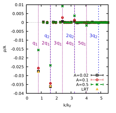
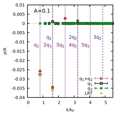
Figure 1: Wave-number dependence of the density response $\braket{\hat{\rho}_{\mathbf{k}}}_{\{\mathbf{q}\},\{A\}}$ for $N_{A}=2$ perturbations with $A_{1}=A_{2}=A$, $\mathbf{q_{1}}=(1,0,0)^{T}2\pi/L$, and $\mathbf{q_{2}}=(2,0,0)^{T}2\pi/L$ for $N=14$ electrons at $r_{s}=2$ and $\theta=1$. Left panel: Response spectrum for different perturbation amplitudes, $A=0.02$ (black squares), $A=0.1$ (red circles), and $A=0.5$ (green crosses). Yellow triangles: LRT. Right panel: Response spectrum for $A=0.1$. Red squares: $\braket{\hat{\rho}_{\mathbf{k}}}_{\{\mathbf{q}\},\{A\}}$ (same as in the left panel); black squares (green crosses): Response for a single perturbation with $\mathbf{q}=\mathbf{q_{1}}$ ($\mathbf{q}=\mathbf{q_{2}}$), taken from Ref. Dornheim et al. (2021d).

Let us start this investigation by considering the full wave-number dependence of the density response for the case of two harmonic perturbations at $r_{s}=2$ and $\theta=1$ shown in Fig. 1. We note that this parameter combination corresponds to a metallic density (e.g. aluminum Sperling et al. (2015)) in the WDM regime, and has frequently been studied in previous investigations Dornheim et al. (2021d, 2020e); Moldabekov et al. (2021a); Dornheim et al. (2021f, e, g); Moldabekov et al. (2021b) of the nonlinear electronic density response. The left panel has been obtained for the case of equal perturbation amplitudes, $A_{1}=A_{2}=A$, and for the two wave numbers $\mathbf{q_{1}}=(1,0,0)^{T}\ 2\pi/L$, and $\mathbf{q_{2}}=(2,0,0)^{T}\ 2\pi/L$. The yellow triangles depict the prediction from LRT, which is given by two independent signals at $\mathbf{q}_{1}$ and $\mathbf{q}_{2}$; any interplay between multiple perturbations is completely neglected.

The black squares have been obtained from our PIMC simulations with a comparably small perturbation amplitude $A=0.02$. In this case, LRT is relatively accurate and the density response is close to zero for all $\mathbf{k}\neq\mathbf{q}_{i}$, although small yet significant signals can be seen at $\mathbf{k}=3\mathbf{q}_{1}$ and $\mathbf{k}=2\mathbf{q}_{2}$. The latter effect is substantially increased for $A=0.1$, as can be seen from the red circles in the same plot. Finally, the green crosses have been obtained for the case of a strong perturbation, $A=0.5$, and the depicted spectrum of the density response strongly deviates from LRT and exhibits at least five different signals.

To understand these nontrivial findings, we have to evaluate the different contributions to the mode-coupled density response given in Eq. (5). Firstly, the first line corresponds to the usual LRT contributions at the original wave numbers $\mathbf{q}_{i}$, which are always present. The second part corresponds to all quadratic contributions, which, in turn, can be further sub-divided into two distinct categories: i) the case $i=j$ gives the quadratic density response at the second harmonic of the respective perturbation. This, too, is not a mode-coupling effect and has been previously reported in Refs. Dornheim et al. (2021d, g); ii) the case $i\neq j$ entails the mode-coupling signal, and predicts a quadratic density response for $\pm\mathbf{k}=\mathbf{q}_{1}\pm\mathbf{q}_{2}$. For the present case, this results in signals at $\mathbf{k}=\mathbf{q}_{1}$ (which comes in addition to the LRT term) and at $\mathbf{k}=3\mathbf{q}_{1}$. In fact, the latter constitutes the dominant nonlinear signal at these parameters, which, too, can be easily understood from Eq. (5). Following the notation from Ref. Dornheim et al. (2021d), the density response at the second harmonic of a perturbation at wave number $\mathbf{q}$ is given by the quadratic density response function $\chi^{(2)}(\mathbf{q})=Y(\mathbf{k}-\mathbf{q},\mathbf{q})\delta_{\mathbf{k},2\mathbf{q}}$. The mode-coupling response at $\mathbf{k}=3\mathbf{q}_{1}$ is instead given by

$$\chi^{(2)}_{\mathbf{q}_{1}+\mathbf{q}_{2}} = Y(\mathbf{k}-\mathbf{q}_{1},\mathbf{q}_{1})\delta_{\mathbf{k},\mathbf{q}_{1}+\mathbf{q}_{2}}$$

$$+ Y(\mathbf{k}-\mathbf{q}_{2},\mathbf{q}_{2})\delta_{\mathbf{k},\mathbf{q}_{1}+\mathbf{q}_{2}}\ ,$$

and thus entails two evaluations of the generalized quadratic response function, namely $Y(\mathbf{q}_{2},\mathbf{q}_{1})$ and $Y(\mathbf{q}_{1},\mathbf{q}_{2})$.

The last effect from the left panel of Fig. 1 that requires an explanation is the signal at $\mathbf{k}=5\mathbf{q}_{1}$ that emerges for strong perturbations, $A=0.5$. Evidently, this has to be a mode-coupling effect, as it is not at an integer harmonic of $\mathbf{q}_{2}$ and would correspond to the fifth harmonic of $\mathbf{q}_{1}$, which is negligible for such parameters Dornheim et al. (2021d). More specifically, it corresponds to a cubic contribution to Eq. (5) at $\mathbf{k}=2\mathbf{q}_{2}+\mathbf{q}_{1}$ that is described by the generalized cubic density response function $Z$.

Let us next consider the right panel of Fig. 1, where we compare the wave number dependence of the density response from different scenarios. Again, the yellow triangles depict the linear response and have been included as a reference. The red circles correspond to the doubly perturbed simulation for $A=0.1$, i.e., the same as the red circles in the left panel. Furthermore, the black squares and green crosses have been obtained from PIMC simulations with only a single perturbation at $\mathbf{q}_{1}$ and $\mathbf{q}_{2}$, respectively, and are taken from Ref. Dornheim et al. (2021d). For the black squares, the signal at the original perturbation can hardly be distinguished from the LRT prediction, whereas the corresponding red circle exhibits a substantially reduced response. Naturally, the latter is a direct consequence of the quadratic mode coupling, as $\mathbf{q}_{1}=\mathbf{q}_{2}-\mathbf{q}_{1}$ in this case. In addition, we find a weak signal at $\mathbf{k}=2\mathbf{q}_{1}$ for the black circles, which is the incipient quadratic response at the second harmonic. The green crosses exhibit a similar behaviour, although the signal at $\mathbf{k}=\mathbf{q}_{2}$ is not as strongly reduced for the double perturbation compared to the other points. This makes sense, as the main deviation of the red circles from LRT is given by the aforementioned contribution from the second harmonic of $\mathbf{q}_{1}$, which is smaller in magnitude than the mode-coupling effect at $\mathbf{k}=\mathbf{q}_{1}$.

In addition, we find a signal at the second harmonic of $\mathbf{q}_{2}$, which is similarly pronounced for both the green crosses and the red circles. Finally, we stress that the signal at $\mathbf{k}=3\mathbf{q}_{1}$ is only present in the simulation of two external perturbations, as it is expected. We thus briefly summarise the following interim conclusions: mode-coupling i) typically constitutes the strongest nonlinear effect as it is comprised of multiple contributions at the same wave number $\mathbf{k}$ [cf. Eq. (III)] and ii) leads to signals at wave numbers where, otherwise, the response would vanish.

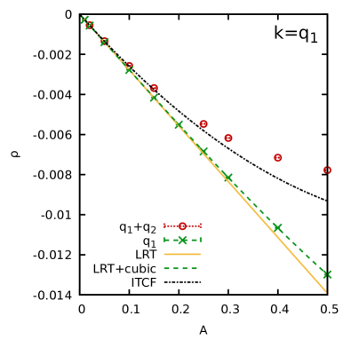
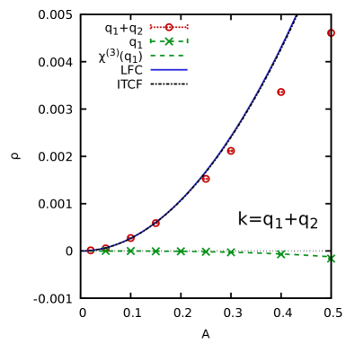
Figure 2: Dependence of the density response at $\mathbf{k}=\mathbf{q}_{1}$ (top) and $\mathbf{k}=\mathbf{q}_{1}+\mathbf{q}_{2}$ (bottom) on the perturbation amplitude $A$ for the same conditions as in Fig. 1. Red circles: PIMC results for the density response at $\mathbf{k}$; dash-dotted black: $A\to 0$ limit predicted by the ITCF, Eq. (II.2); green crosses: PIMC results for the density response at $\mathbf{k}$ from a simulation with a single harmonic potential at $\mathbf{q}_{1}$ taken from Ref. Dornheim et al. (2021d); dashed green: corresponding description based on the cubic density response; solid yellow: LRT; solid blue: LFC-based description of the $A\to 0$ limit from Eq. (II.2).

To provide a more quantitative assessment of the effects due to mode-coupling, we investigate the perturbation amplitude dependence of the density response in Fig. 2. In particular, the top panel corresponds to the case of $\mathbf{k}=\mathbf{q}_{1}$, i.e., at one of the original perturbations, and the red circles show our new PIMC data that have been obtained for the case of two perturbations for different $A$. As a reference, we also include PIMC data from Ref. Dornheim et al. (2021d) that have been obtained for a single perturbation at $\mathbf{q}_{1}$ as the green crosses. The solid yellow line shows the prediction from LRT, which is in good agreement to both PIMC data sets for very small $A$. Strikingly, LRT holds for substantially larger $A$ in the case of a single perturbation compared to the more complicated behaviour due to mode-coupling between $\mathbf{q}_{1}$ and $\mathbf{q}_{2}$. In fact, the dominant nonlinear effect in the green crosses is given by the cubic density response at the first harmonic, which is depicted by the dashed green line, and is in excellent agreement to the data points. In stark contrast, the first nonlinear term in the red circles is quadratic in the perturbation amplitude $A$ and determined by the generalized response function $Y(-\mathbf{q}_{1},\mathbf{q}_{2})=Y(\mathbf{q}_{2},-\mathbf{q}_{1})$. The latter can be conveniently estimated by performing a PIMC simulation of the unperturbed electron gas and evaluating Eq. (II.2); see Ref. Dornheim et al. (2021g) for a detailed description of this procedure. The final result for both LRT and the thus obtained quadratic mode-coupling term is depicted by the dash-dotted black curve, which is in excellent agreement to the independent data points for $A\leq 0.2$. For larger $A$, cubic terms in Eq. (5) start to become noticeable, as it is expected.

The bottom panel of Fig. 2 shows the same information, but for $\mathbf{k}=\mathbf{q}_{1}+\mathbf{q}_{2}$. In this case, the green crosses exhibit a very weak response that is well described by the cubic response of the third harmonic of $\mathbf{q}_{1}$, i.e., the dashed green curve. In stark contrast, the red circles are larger by an order of magnitude and exhibit a parabolic behaviour [cf. Eq. (III)] in leading order that is again well described by the theoretical curve that we obtain by evaluating Eq. (II.2). In addition, the solid blue curve has been obtained by evaluating Eq. (II.2) using as input the static local field correction by Dornheim et al. Dornheim et al. (2020b). Evidently, the resulting parabola is in excellent agreement to the exact $A\to 0$ limit predicted by the ITCF formalism. This, in turn, further corroborates the high value of the LFC for the description of nonlinear effects that has been reported in a previous work Dornheim et al. (2021d).

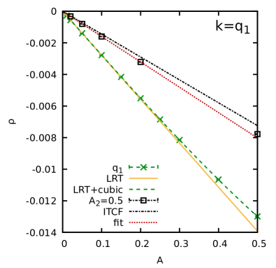
Figure 3: Perturbation strength ($A_{1}$) dependence of the density response at $\mathbf{q_{1}}=(1,0,0)^{T}2\pi/L$ for $r_{s}=2$ and $\theta=1$. A second perturbation at $\mathbf{q_{2}}=(2,0,0)^{T}2\pi/L$ is applied with $A_{2}=0.5$ being fixed. Black squares: PIMC data for the density response at $\mathbf{k}=\mathbf{q}_{1}$; dash-dotted black: ITCF prediction, Eq. (II.2); dotted red: linear fit for $A\leq 0.2$; green crosses: PIMC results for a single external perturbation at $\mathbf{q}_{1}$ taken from Ref. Dornheim et al. (2021d); solid yellow: LRT prediction for the latter case; dashed green: corresponding LRT+cubic response.

A further interesting topic is the behaviour of the density response when the perturbation amplitudes of the two perturbations are not equal. Such a case is investigated in Fig. 3, where we consider the same wave vectors $\mathbf{q}_{1}$ and $\mathbf{q}_{2}$ as before. More specifically, we show the density response at $\mathbf{k}=\mathbf{q}_{1}$, and the $x$-axis shows the perturbation amplitude $A_{1}=A$; the perturbation amplitude $A_{2}=0.5$ is being kept constant. The resulting data are shown as the black squares, and, approximately, exhibit a linear behaviour with $A$. At the same time, the pre-factor substantially differs from the LRT prediction (solid yellow), and from the simulation results obtained for only a single perturbation (green crosses). In other words, we find an apparently linear effect that is not described by LRT.

Yet, this seeming contradiction is resolved by the second line in Eq. (5), which predicts a mode-coupling contribution at $\mathbf{k}=\mathbf{q}_{1}$ that is proportional to $A_{1}\times A_{2}$. Since $A_{2}$ is being kept constant for the results shown in Fig. 3, the quadratic mode-coupling term manifests with a linear dependence on $A_{1}=A$, which resolves this apparent conundrum. The corresponding estimation combining both LRT and the quadratic term that has been obtained from the generalized ITCF [Eq. (II.2)] is depicted as the dash-dotted black line in Fig. 3, and qualitatively captures the correct trend. The comparably small residual differences between data and theory are due to the fact that at $A_{2}=0.5$, even the quadratic description is not fully sufficient; see Fig. 2 above. Finally, the dotted red line has been obtained from a linear fit to the PIMC data for $A\leq 0.2$, and, therefore, depicts the correct nonlinear result for the linear response in this case. We stress that this finding might be of considerable practical relevance, as it directly implies that the presence of a second external perturbation with a large amplitude leads to a break-down of LRT for the first perturbation even in the limit of $A\to 0$. For example, an external ionic potential might be expanded into such harmonics, and the corresponding coefficients might be substantial.

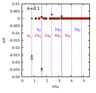
Figure 4: Wave-number dependence of the density response $\braket{\hat{\rho}_{\mathbf{k}}}_{\{\mathbf{q}\},\{A\}}$ at $r_{s}=2$ and $\theta=1$ for $A=0.1$. Black squares: Single perturbation along $\mathbf{q_{1}}=(1,0,0)^{T}2\pi/L$; Green crosses: Single perturbation along $\mathbf{q_{2}}=(2,0,0)^{T}2\pi/L$ . Blue diamonds: two perturbations along $\mathbf{q_{1}}$ and $\mathbf{q_{2}}$. Red circles: two perturbations along $\mathbf{q_{1}}$ and $\mathbf{q_{3}}=(0,2,0)^{T}2\pi/L$. Yellow triangles: LRT.

Let us next consider the impact of the direction of the external perturbation. To this end, we investigate the wave number dependence of the density response again for $r_{s}=2$ and $\theta=1$ in Fig. 4. Specifically, the black squares and green crosses have been obtained for the case of single perturbations along $\mathbf{q}_{1}$ and $\mathbf{q}_{2}$, respectively, with $A=0.1$. In addition, the blue diamonds show the signal for the case of a double perturbation at both $\mathbf{q}_{1}$ and $\mathbf{q}_{2}$ with $A_{1}=A_{2}=A$. Finally, the red circles have been obtained from a new simulation with two perturbations along $\mathbf{q}_{1}$ and $\mathbf{q}_{3}=(0,2,0)^{T}\ 2\pi/L$. We note that the $k$-vectors shown in Fig. 4 have been selected along the $x$-direction insofar as this is possible. Therefore, the red circles are indistinguishable from the black squares as no mode-coupling affects the density response in this direction.

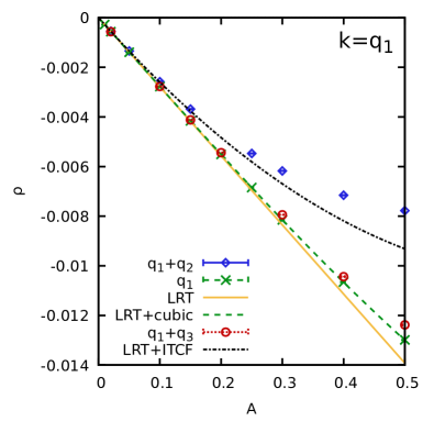
Figure 5: Density response at $\mathbf{q_{1}}=(1,0,0)^{T}2\pi/L$ for the same conditions as in Fig. 4.

This notion is further validated in Fig. 5, where we show the $A$-dependence of the density response at $\mathbf{k}=\mathbf{q}_{1}$. The blue diamonds show the PIMC data for the simulation with two perturbations along $\mathbf{q}_{1}$ and $\mathbf{q}_{2}$, which are well described by LRT and the quadratic mode-coupling response (dash-dotted black curve) as it has been explained before. The green crosses are the simulation results for only a single perturbation at $\mathbf{q}_{1}$, which follow the combination of LRT and the cubic response at the first harmonic. Finally, the red circles have been obtained from the simulations with perturbations at $\mathbf{q}_{1}$ and $\mathbf{q}_{3}$. Evidently, the response at $\mathbf{k}=\mathbf{q}_{1}$ is hardly affected by the presence of the second perturbation along another direction, and the circles closely follow the green crosses for small to medium perturbations. For completeness, we mention that the small deviations at large perturbation amplitudes $A$ are a consequence of cubic mode-coupling terms, cf. Eq. (5).

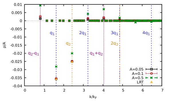
Figure 6: Wave-number dependence of the density response $\braket{\hat{\rho}_{\mathbf{k}}}_{\{\mathbf{q}\},\{A\}}$ at $r_{s}=2$ and $\theta=1$ for two perturbations with $\mathbf{q_{1}}=(2,0,0)^{T}2\pi/L$ and $\mathbf{q_{2}}=(3,0,0)^{T}2\pi/L$, and $A_{1}=A_{2}=A$. Black squares: $A=0.05$; Red circles: $A=0.1$; Green crosses: $A=0.5$; Yellow triangles: LRT.

Let us conclude our study of mode-coupling effects in the density response of the warm dense UEG with a more complicated combination of perturbation wave vectors. This situation is investigated in Fig. 6, where we consider the case of $\mathbf{q}_{1}=(2,0,0)^{T}\ 2\pi/L$ and $\mathbf{q}_{2}=(3,0,0)^{T}\ 2\pi/L$, again with $A_{1}=A_{2}=A$. In particular, the $\mathbf{q}L/2\pi$ are given by prime numbers, so that no quadratic mode-coupling contribution coincides with the original wave numbers or their integer harmonics. As usual, the yellow triangles depict the prediction from LRT, and the black squares, red circles, and green crosses show PIMC results for $A=0.05$, $A=0.1$, and $A=0.5$, respectively.

Evidently, this choice of the $\mathbf{q}_{i}$ results in a number of signals at different wave vectors $\mathbf{k}$ even in the case of a rather weak perturbation, $A=0.05$. More specifically, there appear four quadratic signals (the second harmonics of $\mathbf{q}_{1}$ and $\mathbf{q}_{2}$, and the mode-coupling signals at $\mathbf{k}=\mathbf{q}_{2}\pm\mathbf{q}_{1}$) in addition to the two main peaks at the original wave vectors of the external perturbation. In the regime of large perturbations, $A=0.5$, the situation becomes even more complicated as additional signals occur due to cubic effects. We thus conclude that the density response to a superposition of multiple external perturbations becomes dramatically more complicated beyond the LRT regime.

IV Summary and Discussion

In summary, we have analyzed nonlinear mode-coupling effects in the density response of an electron gas in the WDM regime. This has been achieved on the basis of extensive new ab initio PIMC results that have been obtained by applying multiple external harmonic perturbations at the same time. First and foremost, we note that mode-coupling effects, while being absent in LRT, constitute the dominant nonlinear effect for weak to moderate perturbation amplitudes. In addition, the presence of a strong, constant perturbation at $\mathbf{q_{2}}$ leads to a substantial modification of the linear response at a different wave vector $\mathbf{q}_{1}$ even in the limit of $A\to 0$, which has considerable implications for a non-uniform electron gas in an external potential, for example due to positively charged ions.

From a theoretical perspective, we have shown that mode-coupling effects can be estimated numerically exactly from a PIMC simulation of the unperturbed UEG by computing the generalized imaginary-time correlation functions that have recently been introduced by Dornheim et al. Dornheim et al. (2021g). This leads to a substantial reduction of the computational effort, as, in principle, the full information about mode-coupling between all wave vectors can be obtained from a single simulation.

In addition, we have extended our earlier analytical theory Dornheim et al. (2021d) for the nonlinear density response in terms of the static LFC Dornheim et al. (2019a, 2020b, 2021h), and find excellent agreement between theory and simulations with negligible computational cost.

There exists a large variety of nonlinear response phenomena in WDM. An interesting question is to inquire about the physical origin of the nonlinearity. For example, the Coulomb interaction between the electrons automatically gives rise to nonlinearities: the $1/r$ distance dependence of the Coulomb potential transforms a harmonic perturbation of any particle into a nonlinear response of its neighbors. A familiar example is the generation of high harmonics of a laser field in a gas Schafer et al. (1993). Therefore, our results will be particularly important for situations where the plasma is strongly correlated. While we have studied only moderately coupled warm dense matter ($r_{s}=2$), the consequences will be even more significant when $r_{s}$ is increased. At strong correlations a number of additional nonlinear effects should be expected. For example, modes propagating in different directions may couple if the isotropy of a nonideal system is broken, e.g. in the presence of a magnetic field. Such an effect is known from strongly couple classical plasmas where it leads to nontrivial coupling of transport processes in different directions, including diffusion Ott and Bonitz (2011) and heat transport Ott et al. (2015). Similar nonlinear effects that are mediated by strong Coulomb interaction should also be expected in WDM.

We expect that our new results will open up many avenues for future research in the field of WDM theory and beyond. First and foremost, we mention the potential utility of nonlinear effects in the electronic density response as a method of diagnostics in experiments. Specifically, the interpretation of current X-ray Thomson scattering (XRTS) experiments is solely based on LRT Glenzer and Redmer (2009), and the inference of important plasma parameters such as the electronic temperature $T_{e}$ is notoriously difficult Kraus et al. (2019). In this context, Moldabekov et al. Moldabekov et al. (2021c) have recently suggested that the application of an external perturbation to generate inhomogeneous WDM samples on purpose leads to a modified experimental signal, that more strongly depends on $T_{e}$. Naturally, the accurate theoretical description in this case will have to take into account the mode-coupling between this external potential and the XRTS probe, and the current LFC-based theory is uniquely suited for this endeavour. A second potential application of our work is given by the possibility to use the nonlinear density response as a probe for three- and even four-body correlation functions known from many-body theory Dornheim et al. (2021f), which might give unprecedented insights into the physical mechanisms of WDM. Finally, we mention that a general theory of the nonlinear electronic density response can be directly incorporated into many theoretical approached that have hitherto, often by necessity, been limited to LRT. Prominent examples include the construction of effectively screened ionic potentials Moldabekov et al. (2018, 2019, 2017) and the electronic stopping power Moldabekov et al. (2020). Specifically, going beyond LRT is a crucial step for understanding and exploring the effective ion-ion attraction in the media with strongly correlated electrons Bonev and Ashcroft (2001); Gravel and Ashcroft (2007), which remains to be an unsolved problem Bonitz et al. (2013); Moldabekov et al. (2021d). Additionally, the effect of electronic strong correlations on a projectile energy dissipation (stopping power) is one of the long standing problems in WDM Grabowski et al. (2020); Frenje et al. (2019), which can be addressed using the non-linear response theory Hu and Zaremba (1988).

References

- Loos and Gill (2016) P.-F. Loos and P. M. W. Gill, “The uniform electron gas,” Comput. Mol. Sci 6, 410–429 (2016).
- Giuliani and Vignale (2008) G. Giuliani and G. Vignale, Quantum Theory of the Electron Liquid (Cambridge University Press, Cambridge, 2008).
- Bardeen et al. (1957) J. Bardeen, L. N. Cooper, and J. R. Schrieffer, “Theory of superconductivity,” Phys. Rev. 108, 1175–1204 (1957).
- Ceperley and Alder (1980) D. M. Ceperley and B. J. Alder, “Ground state of the electron gas by a stochastic method,” Phys. Rev. Lett. 45, 566–569 (1980).
- Moroni et al. (1995) S. Moroni, D. M. Ceperley, and G. Senatore, “Static response and local field factor of the electron gas,” Phys. Rev. Lett 75, 689 (1995).
- Spink et al. (2013) G. G. Spink, R. J. Needs, and N. D. Drummond, “Quantum monte carlo study of the three-dimensional spin-polarized homogeneous electron gas,” Phys. Rev. B 88, 085121 (2013).
- Jones (2015) R. O. Jones, “Density functional theory: Its origins, rise to prominence, and future,” Rev. Mod. Phys. 87, 897–923 (2015).
- Dornheim et al. (2018a) T. Dornheim, S. Groth, and M. Bonitz, “The uniform electron gas at warm dense matter conditions,” Phys. Reports 744, 1–86 (2018a).
- Fortov (2009) V. E. Fortov, “Extreme states of matter on earth and in space,” Phys.-Usp 52, 615–647 (2009).
- Vorberger et al. (2007) J. Vorberger, I. Tamblyn, B. Militzer, and S. A. Bonev, “Hydrogen-helium mixtures in the interiors of giant planets,” Phys. Rev. B 75, 024206 (2007).
- Militzer et al. (2008) B. Militzer, W. B. Hubbard, J. Vorberger, I. Tamblyn, and S. A. Bonev, “A massive core in jupiter predicted from first-principles simulations,” The Astrophysical Journal 688, L45–L48 (2008).
- Becker et al. (2014) A. Becker, W. Lorenzen, J. J. Fortney, N. Nettelmann, M. Schöttler, and R. Redmer, “Ab initio equations of state for hydrogen (h-reos.3) and helium (he-reos.3) and their implications for the interior of brown dwarfs,” Astrophys. J. Suppl. Ser 215, 21 (2014).
- Saumon et al. (1992) D. Saumon, W. B. Hubbard, G. Chabrier, and H. M. van Horn, “The role of the molecular-metallic transition of hydrogen in the evolution of jupiter, saturn, and brown dwarfs,” Astrophys. J 391, 827–831 (1992).
- Hu et al. (2011) S. X. Hu, B. Militzer, V. N. Goncharov, and S. Skupsky, “First-principles equation-of-state table of deuterium for inertial confinement fusion applications,” Phys. Rev. B 84, 224109 (2011).
- Brongersma et al. (2015) Mark L. Brongersma, Naomi J. Halas, and Peter Nordlander, “Plasmon-induced hot carrier science and technology,” Nature Nanotechnology 10, 25–34 (2015).
- Falk (2018) K. Falk, “Experimental methods for warm dense matter research,” High Power Laser Sci. Eng 6, e59 (2018).
- Brown et al. (2013) Ethan W. Brown, Bryan K. Clark, Jonathan L. DuBois, and David M. Ceperley, “Path-integral monte carlo simulation of the warm dense homogeneous electron gas,” Phys. Rev. Lett. 110, 146405 (2013).
- Malone et al. (2016) Fionn D. Malone, N. S. Blunt, Ethan W. Brown, D. K. K. Lee, J. S. Spencer, W. M. C. Foulkes, and James J. Shepherd, “Accurate exchange-correlation energies for the warm dense electron gas,” Phys. Rev. Lett. 117, 115701 (2016).
- Dornheim et al. (2016a) T. Dornheim, S. Groth, T. Sjostrom, F. D. Malone, W. M. C. Foulkes, and M. Bonitz, “Ab initio quantum Monte Carlo simulation of the warm dense electron gas in the thermodynamic limit,” Phys. Rev. Lett. 117, 156403 (2016a).
- Dornheim et al. (2017a) Tobias Dornheim, Simon Groth, Fionn D. Malone, Tim Schoof, Travis Sjostrom, W. M. C. Foulkes, and Michael Bonitz, “Ab initio quantum Monte Carlo simulation of the warm dense electron gas,” Phys. Plasmas 24, 056303 (2017a), https://doi.org/10.1063/1.4977920 .
- Dornheim et al. (2015) Tobias Dornheim, Tim Schoof, Simon Groth, Alexey Filinov, and Michael Bonitz, “Permutation blocking path integral Monte Carlo approach to the uniform electron gas at finite temperature,” J. Chem. Phys. 143, 204101 (2015).
- Dornheim et al. (2016b) T. Dornheim, S. Groth, T. Schoof, C. Hann, and M. Bonitz, “Ab initio quantum Monte Carlo simulations of the uniform electron gas without fixed nodes: The unpolarized case,” Phys. Rev. B 93, 205134 (2016b).
- Groth et al. (2016) S. Groth, T. Schoof, T. Dornheim, and M. Bonitz, “Ab initio quantum Monte Carlo simulations of the uniform electron gas without fixed nodes,” Phys. Rev. B 93, 085102 (2016).
- Schoof et al. (2015) T. Schoof, S. Groth, J. Vorberger, and M. Bonitz, “Ab Initio thermodynamic results for the degenerate electron gas at finite temperature,” Phys. Rev. Lett. 115, 130402 (2015).
- Lee et al. (2021) Joonho Lee, Miguel A. Morales, and Fionn D. Malone, “A phaseless auxiliary-field quantum monte carlo perspective on the uniform electron gas at finite temperatures: Issues, observations, and benchmark study,” The Journal of Chemical Physics 154, 064109 (2021), https://doi.org/10.1063/5.0041378 .
- Groth et al. (2017a) S. Groth, T. Dornheim, T. Sjostrom, F. D. Malone, W. M. C. Foulkes, and M. Bonitz, “Ab initio exchange–correlation free energy of the uniform electron gas at warm dense matter conditions,” Phys. Rev. Lett. 119, 135001 (2017a).
- Karasiev et al. (2014) Valentin V. Karasiev, Travis Sjostrom, James Dufty, and S. B. Trickey, “Accurate homogeneous electron gas exchange-correlation free energy for local spin-density calculations,” Phys. Rev. Lett. 112, 076403 (2014).
- Karasiev et al. (2019) Valentin V. Karasiev, S. B. Trickey, and James W. Dufty, “Status of free-energy representations for the homogeneous electron gas,” Phys. Rev. B 99, 195134 (2019).
- Karasiev et al. (2016) V. V. Karasiev, L. Calderin, and S. B. Trickey, “Importance of finite-temperature exchange correlation for warm dense matter calculations,” Phys. Rev. E 93, 063207 (2016).
- Ramakrishna et al. (2020) Kushal Ramakrishna, Tobias Dornheim, and Jan Vorberger, “Influence of finite temperature exchange-correlation effects in hydrogen,” Phys. Rev. B 101, 195129 (2020).
- Dornheim et al. (2017b) Tobias Dornheim, Simon Groth, and Michael Bonitz, “Ab initio results for the static structure factor of the warm dense electron gas,” Contrib. Plasma Phys. 57, 468–478 (2017b).
- Dornheim et al. (2020a) Tobias Dornheim, Jan Vorberger, and Michael Bonitz, “Nonlinear electronic density response in warm dense matter,” Phys. Rev. Lett. 125, 085001 (2020a).
- Dornheim et al. (2020b) Tobias Dornheim, Attila Cangi, Kushal Ramakrishna, Maximilian Böhme, Shigenori Tanaka, and Jan Vorberger, “Effective static approximation: A fast and reliable tool for warm-dense matter theory,” Phys. Rev. Lett. 125, 235001 (2020b).
- Militzer et al. (2019) B. Militzer, E.L. Pollock, and D.M. Ceperley, “Path integral monte carlo calculation of the momentum distribution of the homogeneous electron gas at finite temperature,” High Energy Density Physics 30, 13–20 (2019).
- Hunger et al. (2020) Kai Hunger, Tim Schoof, Tobias Dornheim, Simon Groth, and Michael Bonitz, “Short-range correlations and momentum distribution function of the warm dense electron gas – ab initio quantum Monte Carlo results,” to be published (2020).
- Dornheim et al. (2021a) Tobias Dornheim, Maximilian Böhme, Burkhard Militzer, and Jan Vorberger, “Ab initio path integral monte carlo approach to the momentum distribution of the uniform electron gas at finite temperature without fixed nodes,” Phys. Rev. B 103, 205142 (2021a).
- Dornheim et al. (2021b) Tobias Dornheim, Jan Vorberger, Burkhard Militzer, and Zhandos A. Moldabekov, “Momentum distribution of the uniform electron gas at finite temperature: Effects of spin-polarization,” (2021b), arXiv:2106.00973 [physics.comp-ph] .
- Militzer and Pollock (2002) Burkhard Militzer and E. L. Pollock, “Lowering of the kinetic energy in interacting quantum systems,” Phys. Rev. Lett. 89, 280401 (2002).
- Dornheim et al. (2018b) T. Dornheim, S. Groth, J. Vorberger, and M. Bonitz, “Ab initio path integral Monte Carlo results for the dynamic structure factor of correlated electrons: From the electron liquid to warm dense matter,” Phys. Rev. Lett. 121, 255001 (2018b).
- Groth et al. (2019) S. Groth, T. Dornheim, and J. Vorberger, “Ab initio path integral Monte Carlo approach to the static and dynamic density response of the uniform electron gas,” Phys. Rev. B 99, 235122 (2019).
- Dornheim and Vorberger (2020) Tobias Dornheim and Jan Vorberger, “Finite-size effects in the reconstruction of dynamic properties from ab initio path integral monte carlo simulations,” Phys. Rev. E 102, 063301 (2020).
- Hamann et al. (2020a) Paul Hamann, Tobias Dornheim, Jan Vorberger, Zhandos Moldabekov, and Michael Bonitz, “Dynamic Properties of the warm dense Electron gas: an ab initio path integral Monte Carlo approach,” submitted for publication (2020a).
- Hamann et al. (2020b) Paul Hamann, Tobas Dornheim, Jan Vorberger, Zhandos Moldabekov, and Michael Bonitz, “Ab initio results for the plasmon dispersion and damping of the warm dense electron gas,” Contributions to Plasma Physics (2020b).
- Kraus et al. (2019) D. Kraus, B. Bachmann, B. Barbrel, R. W. Falcone, L. B. Fletcher, S. Frydrych, E. J. Gamboa, M. Gauthier, D. O. Gericke, S. H. Glenzer, S. Göde, E. Granados, N. J. Hartley, J. Helfrich, H. J. Lee, B. Nagler, A. Ravasio, W. Schumaker, J. Vorberger, and T. Döppner, “Characterizing the ionization potential depression in dense carbon plasmas with high-precision spectrally resolved x-ray scattering,” Plasma Phys. Control Fusion 61, 014015 (2019).
- Glenzer and Redmer (2009) S. H. Glenzer and R. Redmer, “X-ray thomson scattering in high energy density plasmas,” Rev. Mod. Phys 81, 1625 (2009).
- Senatore et al. (1996) G. Senatore, S. Moroni, and D. M. Ceperley, “Local field factor and effective potentials in liquid metals,” J. Non-Cryst. Sol 205-207, 851–854 (1996).
- Moldabekov et al. (2020) Zh. A. Moldabekov, T. Dornheim, M. Bonitz, and T. S. Ramazanov, “Ion energy-loss characteristics and friction in a free-electron gas at warm dense matter and nonideal dense plasma conditions,” Phys. Rev. E 101, 053203 (2020).
- Moroni et al. (1992) S. Moroni, D. M. Ceperley, and G. Senatore, “Static response from quantum Monte Carlo calculations,” Phys. Rev. Lett 69, 1837 (1992).
- Corradini et al. (1998) M. Corradini, R. Del Sole, G. Onida, and M. Palummo, “Analytical expressions for the local-field factor and the exchange-correlation kernel of the homogeneous electron gas,” Phys. Rev. B 57, 14569 (1998).
- Dornheim et al. (2019a) T. Dornheim, J. Vorberger, S. Groth, N. Hoffmann, Zh.A. Moldabekov, and M. Bonitz, “The static local field correction of the warm dense electron gas: An ab initio path integral Monte Carlo study and machine learning representation,” J. Chem. Phys 151, 194104 (2019a).
- Dornheim et al. (2020c) Tobias Dornheim, Travis Sjostrom, Shigenori Tanaka, and Jan Vorberger, “Strongly coupled electron liquid: Ab initio path integral monte carlo simulations and dielectric theories,” Phys. Rev. B 101, 045129 (2020c).
- Dornheim et al. (2020d) Tobias Dornheim, Zhandos A Moldabekov, Jan Vorberger, and Simon Groth, “Ab initio path integral monte carlo simulation of the uniform electron gas in the high energy density regime,” Plasma Physics and Controlled Fusion 62, 075003 (2020d).
- Castello et al. (2021) F. Lucco Castello, P. Tolias, and T. Dornheim, “Classical bridge functions in classical and quantum plasma liquids,” (2021), arXiv:2107.03537 [physics.plasm-ph] .
- Dornheim et al. (2021c) Tobias Dornheim, Zhandos A. Moldabekov, and Panagiotis Tolias, “Analytical representation of the local field correction of the uniform electron gas within the effective static approximation,” Phys. Rev. B 103, 165102 (2021c).
- Dornheim et al. (2020e) Tobias Dornheim, Jan Vorberger, and Michael Bonitz, “Nonlinear Electronic Density Response in Warm Dense Matter,” Phys. Rev. Lett. 125, 085001 (2020e).
- Dornheim et al. (2021d) Tobias Dornheim, Maximilian Böhme, Zhandos A. Moldabekov, Jan Vorberger, and Michael Bonitz, “Density response of the warm dense electron gas beyond linear response theory: Excitation of harmonics,” Phys. Rev. Research 3, 033231 (2021d).
- Dornheim et al. (2021e) Tobias Dornheim, Zhandos A. Moldabekov, and Jan Vorberger, “Nonlinear electronic density response of the ferromagnetic uniform electron gas at warm dense matter conditions,” Contributions to Plasma Physics , e202100098 (2021e).
- Dornheim et al. (2017c) Tobias Dornheim, Simon Groth, Jan Vorberger, and Michael Bonitz, “Permutation-blocking path-integral Monte Carlo approach to the static density response of the warm dense electron gas,” Phys. Rev. E 96, 023203 (2017c).
- Groth et al. (2017b) Simon Groth, Tobias Dornheim, and Michael Bonitz, “Configuration path integral Monte Carlo approach to the static density response of the warm dense electron gas,” J. Chem. Phys. 147, 164108 (2017b).
- Bowen et al. (1994) C. Bowen, G. Sugiyama, and B. J. Alder, “Static dielectric response of the electron gas,” Phys. Rev. B 50, 14838 (1994).
- Fletcher et al. (2015) L. B. Fletcher, H. J. Lee, T. Döppner, E. Galtier, B. Nagler, P. Heimann, C. Fortmann, S. LePape, T. Ma, M. Millot, A. Pak, D. Turnbull, D. A. Chapman, D. O. Gericke, J. Vorberger, T. White, G. Gregori, M. Wei, B. Barbrel, R. W. Falcone, C.-C. Kao, H. Nuhn, J. Welch, U. Zastrau, P. Neumayer, J. B. Hastings, and S. H. Glenzer, “Ultrabright x-ray laser scattering for dynamic warm dense matter physics,” Nature Photonics 9, 274–279 (2015).
- Dornheim et al. (2021f) Tobias Dornheim, Jan Vorberger, and Zhandos A. Moldabekov, “Nonlinear density response and higher order correlation functions in warm dense matter,” Journal of the Physical Society of Japan 90, 104002 (2021f).
- Dornheim et al. (2021g) Tobias Dornheim, Zhandos A. Moldabekov, and Jan Vorberger, “Nonlinear density response from imaginary-time correlation functions: Ab initio path integral monte carlo simulations of the warm dense electron gas,” The Journal of Chemical Physics 155, 054110 (2021g).
- Hartmann et al. (2018) N. Hartmann, G. Hartmann, R. Heider, M. S. Wagner, M. Ilchen, J. Buck, A. O. Lindahl, C. Benko, J. Grünert, J. Krzywinski, J. Liu, A. A. Lutman, A. Marinelli, T. Maxwell, A. A. Miahnahri, S. P. Moeller, M. Planas, J. Robinson, A. K. Kazansky, N. M. Kabachnik, J. Viefhaus, T. Feurer, R. Kienberger, R. N. Coffee, and W. Helml, “Attosecond time–energy structure of x-ray free-electron laser pulses,” Nature Photonics 12, 215–220 (2018).
- Ott, Torben et al. (2018) Ott, Torben, Thomsen, Hauke, Abraham, Jan Willem, Dornheim, Tobias, and Bonitz, Michael, “Recent progress in the theory and simulation of strongly correlated plasmas: phase transitions, transport, quantum, and magnetic field effects,” Eur. Phys. J. D 72, 84 (2018).
- Drummond et al. (2004) N. D. Drummond, Z. Radnai, J. R. Trail, M. D. Towler, and R. J. Needs, “Diffusion quantum monte carlo study of three-dimensional wigner crystals,” Phys. Rev. B 69, 085116 (2004).
- Ceperley (1995) D. M. Ceperley, “Path integrals in the theory of condensed helium,” Rev. Mod. Phys 67, 279 (1995).
- Dornheim et al. (2019b) T. Dornheim, S. Groth, A. V. Filinov, and M. Bonitz, “Path integral monte carlo simulation of degenerate electrons: Permutation-cycle properties,” The Journal of Chemical Physics 151, 014108 (2019b), https://doi.org/10.1063/1.5093171 .
- Troyer and Wiese (2005) M. Troyer and U. J. Wiese, “Computational complexity and fundamental limitations to fermionic quantum Monte Carlo simulations,” Phys. Rev. Lett 94, 170201 (2005).
- Dornheim (2019) T. Dornheim, “Fermion sign problem in path integral Monte Carlo simulations: Quantum dots, ultracold atoms, and warm dense matter,” Phys. Rev. E 100, 023307 (2019).
- Dornheim (2021) Tobias Dornheim, “Fermion sign problem in path integral monte carlo simulations: grand-canonical ensemble,” Journal of Physics A: Mathematical and Theoretical 54, 335001 (2021).
- Nolting and Brewer (2009) W. Nolting and W. D. Brewer, Fundamentals of Many-body Physics: Principles and Methods (Springer, Heidelberg, 2009).
- Hu and Zaremba (1988) C. D. Hu and E. Zaremba, “ correction to the stopping power of ions in an electron gas,” Phys. Rev. B 37, 9268–9277 (1988).
- Mezzacapo and Boninsegni (2007) F. Mezzacapo and M. Boninsegni, “Structure, superfluidity, and quantum melting of hydrogen clusters,” Phys. Rev. A 75, 033201 (2007).
- Boninsegni et al. (2006a) M. Boninsegni, N. V. Prokofev, and B. V. Svistunov, “Worm algorithm and diagrammatic Monte Carlo: A new approach to continuous-space path integral Monte Carlo simulations,” Phys. Rev. E 74, 036701 (2006a).
- Boninsegni et al. (2006b) M. Boninsegni, N. V. Prokofev, and B. V. Svistunov, “Worm algorithm for continuous-space path integral Monte Carlo simulations,” Phys. Rev. Lett 96, 070601 (2006b).
- Sperling et al. (2015) P. Sperling, E. J. Gamboa, H. J. Lee, H. K. Chung, E. Galtier, Y. Omarbakiyeva, H. Reinholz, G. Röpke, U. Zastrau, J. Hastings, L. B. Fletcher, and S. H. Glenzer, “Free-electron x-ray laser measurements of collisional-damped plasmons in isochorically heated warm dense matter,” Phys. Rev. Lett. 115, 115001 (2015).
- Moldabekov et al. (2021a) Zhandos Moldabekov, Tobias Dornheim, Maximilian Böhme, Jan Vorberger, and Attila Cangi, “The relevance of electronic perturbations in the warm dense electron gas,” The Journal of Chemical Physics 155, 124116 (2021a).
- Moldabekov et al. (2021b) Zhandos Moldabekov, Tobias Dornheim, Jan Vorberger, and Attila Cangi, “Benchmarking exchange-correlation functionals in the spin-polarized inhomogeneous electron gas under warm dense conditions,” (2021b), arXiv:2110.06708 [physics.plasm-ph] .
- Dornheim et al. (2021h) Tobias Dornheim, Zhandos A. Moldabekov, and Panagiotis Tolias, “Analytical representation of the local field correction of the uniform electron gas within the effective static approximation,” Phys. Rev. B 103, 165102 (2021h).
- Schafer et al. (1993) K. J. Schafer, Baorui Yang, L. F. DiMauro, and K. C. Kulander, “Above threshold ionization beyond the high harmonic cutoff,” Phys. Rev. Lett. 70, 1599–1602 (1993).
- Ott and Bonitz (2011) T. Ott and M. Bonitz, “Diffusion in a strongly coupled magnetized plasma,” Phys. Rev. Lett. 107, 135003 (2011).
- Ott et al. (2015) T. Ott, M. Bonitz, and Z. Donkó, “Effect of correlations on heat transport in a magnetized strongly coupled plasma,” Phys. Rev. E 92, 063105 (2015).
- Moldabekov et al. (2021c) Zh. A. Moldabekov, T. Dornheim, and A. Cangi, “Thermal signals from collective electronic excitations in inhomogeneous warm dense matter,” (2021c), arXiv:2105.09721 [physics.plasm-ph] .
- Moldabekov et al. (2018) Zh.A. Moldabekov, S. Groth, T. Dornheim, H. Kählert, M. Bonitz, and T. S. Ramazanov, “Structural characteristics of strongly coupled ions in a dense quantum plasma,” Phys. Rev. E 98, 023207 (2018).
- Moldabekov et al. (2019) Zh.A. Moldabekov, H. Kählert, T. Dornheim, S. Groth, M. Bonitz, and T. S. Ramazanov, “Dynamical structure factor of strongly coupled ions in a dense quantum plasma,” Phys. Rev. E 99, 053203 (2019).
- Moldabekov et al. (2017) Zh.A. Moldabekov, S. Groth, T. Dornheim, M. Bonitz, and T.S. Ramazanov, “Ion potential in non-ideal dense quantum plasmas,” Contributions to Plasma Physics 57, 532–538 (2017).
- Bonev and Ashcroft (2001) S. A. Bonev and N. W. Ashcroft, “Hydrogen in jellium: First-principles pair interactions,” Phys. Rev. B 64, 224112 (2001).
- Gravel and Ashcroft (2007) Simon Gravel and N. W. Ashcroft, “Nonlinear response theories and effective pair potentials,” Phys. Rev. B 76, 144103 (2007).
- Bonitz et al. (2013) M. Bonitz, E. Pehlke, and T. Schoof, “Attractive forces between ions in quantum plasmas: Failure of linearized quantum hydrodynamics,” Phys. Rev. E 87, 033105 (2013).
- Moldabekov et al. (2021d) Zhandos A. Moldabekov, Tobias Dornheim, and Michael Bonitz, “Screening of a test charge in a free-electron gas at warm dense matter and dense non-ideal plasma conditions,” Contributions to Plasma Physics , e202000176 (2021d).
- Grabowski et al. (2020) P.E. Grabowski, S.B. Hansen, M.S. Murillo, L.G. Stanton, F.R. Graziani, A.B. Zylstra, S.D. Baalrud, P. Arnault, A.D. Baczewski, L.X. Benedict, C. Blancard, O. Čertík, J. Clérouin, L.A. Collins, S. Copeland, A.A. Correa, J. Dai, J. Daligault, M.P. Desjarlais, M.W.C. Dharma-wardana, G. Faussurier, J. Haack, T. Haxhimali, A. Hayes-Sterbenz, Y. Hou, S.X. Hu, D. Jensen, G. Jungman, G. Kagan, D. Kang, J.D. Kress, Q. Ma, M. Marciante, E. Meyer, R.E. Rudd, D. Saumon, L. Shulenburger, R.L. Singleton, T. Sjostrom, L.J. Stanek, C.E. Starrett, C. Ticknor, S. Valaitis, J. Venzke, and A. White, “Review of the first charged-particle transport coefficient comparison workshop,” High Energy Density Physics 37, 100905 (2020).
- Frenje et al. (2019) J. A. Frenje, R. Florido, R. Mancini, T. Nagayama, P. E. Grabowski, H. Rinderknecht, H. Sio, A. Zylstra, M. Gatu Johnson, C. K. Li, F. H. Séguin, R. D. Petrasso, V. Yu Glebov, and S. P. Regan, “Experimental validation of low- ion-stopping formalisms around the bragg peak in high-energy-density plasmas,” Phys. Rev. Lett. 122, 015002 (2019).