Conductance and Social Capital: Modeling and Empirically Measuring Online Social Influence

Abstract.

Social influence pervades our everyday lives and lays the foundation for complex social phenomena, such as the spread of misinformation and the polarization of communities. In a crisis like the COVID-19 pandemic, social influence can determine whether life-saving information is adopted, public health measures are observed, or immunization campaigns meet their targets. Existing literature studying online social influence suffers from several drawbacks. First, a disconnect appears between psychology approaches, which are generally performed and tested in controlled lab experiments, and the quantitative methods, which are usually data-driven and rely on network and event analysis. The former are slow, expensive to deploy, and typically do not generalize well to topical issues (such as an ongoing pandemic); the latter often oversimplify the complexities of social influence and ignore psychosocial literature. This work bridges this gap and presents three contributions towards modeling and empirically quantifying online influence. The first contribution is a data-driven Generalized Influence Model that incorporates two novel psychosocial-inspired mechanisms: the conductance of the diffusion network and the social capital distribution. The second contribution is a framework to empirically rank users’ social influence using a human-in-the-loop active learning method combined with crowdsourced pairwise influence comparisons. We build a human-labeled ground truth, calibrate our generalized influence model and perform a large-scale evaluation of influence. We find that our generalized model outperforms the current state-of-the-art approaches and corrects the inherent biases introduced by the widely used follower count. As the third contribution, we apply the influence model to discussions around COVID-19. We quantify users’ influence, and we tabulate it against their professions. We find that the executives, media, and military are more influential than pandemic-related experts such as life scientists and healthcare professionals. These findings call on such professionals to own up to their responsibility for shaping social reactions.

1. Introduction

Influence is foundational to the construction of opinions and enacting change. It governs interpersonal relationships and contributes to the establishment of societal institutions and reforms (Nowak et al., 2005). Social media ubiquity provides fertile ground for influence mechanisms to unfold and for a minority of users to exert disproportionate control. Although there is a rich trove of literature related to social influence, stretching from the psychosocial to computational domains, a quantitative approach to measuring online influence remains elusive (Peng et al., 2018; Mason et al., 2007). Successful solutions to this problem would allow identifying the online actors who shape societal views and would also be a first step toward addressing societal issues—such as the spreading of misinformation amid a pandemic that undermines immunization campaigns and stokes vaccine hesitancy.

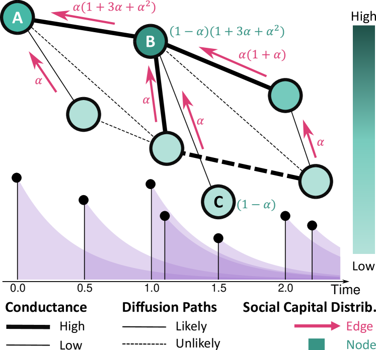
Figure 1. Schema of the Generalized Influence Model (GIM). (bottom) An example cascade is modeled using Hawkes processes. Each event (timestamp on x-axis) has a mark (y-axis) and spawns new events following a time-decaying intensity (magenta areas). (top) The latent branching structure is shown with solid lines, and other valid pathways are shown with dotted lines. GIM has two psychosocial-inspired components. Conductance: Edge thickness represents conductance, which modulates the likelihood of observing diffusions along that edge. Social capital distribution: A percentage $\alpha$ of a node’s capital (green shades) is transferred along diffusion edges (red arrows), from target to source. Influence is proportional to the accumulated capital.

In this paper, we model and empirically measure online influence by bridging the divide between psychology and the quantitative approaches (Asch, 1961). The psychology approaches (Asch, 1961; Milgram and Gudehus, 1978; Cialdini, 2001) involve micro-level analysis in well-controlled laboratory experiments. Such works understand minute factors and infer causal relationships. Still, they are slow, expensive to deploy, and cannot be leveraged in real-time (say to analyze influence in pandemic-related discussions). The quantitative approaches (Cha et al., 2010; Rizoiu et al., 2018; Du et al., 2013a) scale to large networks and model the emergent behavior therein. However, these are usually data-driven tools that make “empirically questionable simplifying assumptions” (Mason et al., 2007). Such operationalizations only offer narrow interpretations of influence and often evaluate against on-hand metrics (for example, retweet counts) that are weak and biased influence representations (see our results in Section 4.2).

In this work, we address several open questions relating to modeling empirical influence. The first question concerns quantitatively modeling and estimating influence from online conversations data. The conductance ((Cialdini, 2001; Newcomb, 1953), see Section 3.1.1) and social attribution ((Milgram and Gudehus, 1978; Horai et al., 1974; Cialdini, 2001), see Section 3.1.2) are known in psychosocial literature to modulate the exertion of social influence. However, these factors are not considered by quantitative models. For conductance, these models often assume that social ties are the primary influence channels, while other conductive channels (like recommender systems and homophily) are underexplored. For social attribution, the question is who gets the (social) credit in a chain of influence exertion. Consider the example in Fig. 1. Alice influences Bobbie, who influences several people; should Alice (the initiator) or Bobbie (the connector) be attributed more social capital? Therefore, we ask how do we model influence to account for network conductance and social attribution mechanisms?

The second question relates to empirically measuring influence at scale. Psychological studies mainly concentrate on identifying the characteristics that allow individuals to exert influence – such as authority, likeability, attractiveness, and expertise (Cialdini, 2001). However, such works deal less with measuring relative influence between individuals and the emergence of social capital (defined as the confluence of said influence-enabling characteristics). Furthermore, performing pairwise comparisons between individuals scales quadratically with the size of the cohort, quickly rendering the costs prohibitive and keeping the size of the studies small. Additionally, without laboratory-controlled environments, data fidelity can suffer. Therefore, how do we generate an empirical social capital ranking, true to the complexities of social influence, and scale it feasibly to large cohorts?

The third question concerns the exertion of influence within discussions with societal stakes (here, the COVID-19 pandemic). Ideally, populations would heed the advice of experts (i.e., epidemiologists, biomedical scientists, and healthcare professionals) during pandemics; however, the rise of the anti-vaxxer movement and vaccine hesitancy is evidence to the contrary. The question is can we identify the occupational groups which yield the most influence in the discussions around the COVID-19 crisis?

We address the above questions on two Twitter datasets about the Australian ‘Black Summer’ Bushfires and the COVID-19 pandemic.

We address the first question by proposing the Generalized Influence Model (GIM) that quantifies influence based on observed information cascades. It leverages two psychosocial-inspired components, depicted in Fig. 1. The conductance mechanism modulates the likelihood of cascade pathways using user lexical and following similarity, and relationship ties. The social capital distribution mechanism transfers a proportion of a node’s social capital to its parent in the information cascade, allowing highly connected nodes to accumulate social capital (which translates to influence).

We address the second question by constructing a crowdsource-based empirical influence measurement framework containing three components. First, we use a human-in-the-loop active learning technique that selects a minimal number of pairwise comparisons to be made and maximizes the utility of each decision. Second, we leverage an augmented Bradley-Terry model to build an influence ranking from pairwise comparisons while accounting for systematic noise in worker decisions. Third, we engineer an MTurk survey instrument; we use an ablation study to estimate the impact of design features on the worker decision accuracy. We design simulation and parameter fitting tools to estimate the budget required to scale the MTurk experiment given a number of targets. We use the MTurk empirical influence estimation to construct a ground truth for evaluation. We show GIM to outperform several baselines, including the current state-of-the-art influence quantification (Rizoiu et al., 2018), and to correct the biases introduced by the widely used follower count.

We address the last question by applying GIM to estimate users’ influence in a large dataset of COVID-19 discussions. We determine user occupation using the O*NET taxonomy (for O*NET Development, [n.d.]), and find that executives and the media are the most influential occupations, while engineers and computer specialists are the least influential. Worryingly, the pandemic experts and healthcare workers are less influential than food processors, entertainers, and business professionals in pandemic-related discussions.

The main contributions of this work include:

• A Generalized Influence Model which incorporates two novel psychosocial-inspired mechanisms: conductance and social capital distribution.

• A crowdsourced empirical influence measurement framework to build the influence ranking of large cohorts.

• Quantifying the influence of occupational groups in COVID-19 related discussions and finding (perhaps unsurprisingly) that pandemic experts are not the most influential.

2. Preliminaries

This section briefly introduces the prerequisites for this work. In Section 2.1, we link social influence and modeling diffusion cascades using the Hawkes self-exciting model. In Section 2.2, we cover the empirical psychometric measurement pipeline, including the use the pairwise comparisons, ranking from pairwise data, and practicalities of collecting pairwise data online.

2.1. Hawkes-modeled Influence

The retweet—Twitter’s affordance to share others’ tweets (and retweets)—is widely seen as an explicit endorsement of opinions and ideas. Consequently, prior works define a tweet’s influence as the number of (direct and indirect) retweets it generates (Du et al., 2013b; Rizoiu et al., 2018). However, the branching structure of retweet cascades is unobserved as Twitter attributes all retweets to the original tweet. Rizoiu et al. (2018) infer it by assuming retweets arrive following a Hawkes point process.

Retweet cascades consist of an original tweet and the subsequent retweets. We denote a marked cascade up to time $T$ as $\operatorname{\mathcal{H}}_{\zeta}(T)=\{v_{1},v_{2},\ldots\}$, where $v_{i}=(t_{i},\zeta_{i})$ denotes the $i$th tweet, $t_{i}$ is the event time relative to the original tweet ($t_{1}=0$), and $\zeta_{i}\in\mathbb{R}$—dubbed the mark—is the event meta-data. The branching structure of retweet cascades is a latent graph $(G,E)$ where $G$ are the tweets, and $E$ contains direct retweet relations. Given a cascade of $n$ events, we define the set of all valid branching structures as $\Upsilon=\{G|(v_{i},v_{j})\in G\text{ so that }t_{i}<t_{j}\}$. Rizoiu et al. (2018) show that $|\Upsilon|=(n-1)!$. Fig. 1 shows an example retweet cascade, its most likely branching structure in solid lines and other potential branching structures in dashed lines. Next, we compute the probability mass function over the branching structure set $\Upsilon$.

Hawkes Processes (Hawkes, 1971) are stochastic processes with the self-exciting property—the arrival of an event increases the likelihood of future events—, applicable here due to the property of social affirmation (i.e., past social actions encourage incoming actions). In Hawkes processes, events arrive following the conditional intensity

$$\lambda(t|\operatorname{\mathcal{H}}_{\zeta}(t))=\mu(t)+\sum_{v_{i}\in\operatorname{\mathcal{H}}_{\zeta}(t):t_{i}<t}\zeta_{i}^{b}\phi(t-t_{i})\enspace,$$

where $\mu(t)$ is the baseline intensity; each event $v_{i}$ increases the overall intensity by $\zeta_{i}^{b}\phi(t-t_{i})$; $\zeta_{i}^{b}$ is one way to model marks where $b$ mediates the marks’ effect, and the kernel $\phi:\mathbb{R}^{+}\rightarrow\mathbb{R}^{+}$ controls the event intensity decay. The exponential $\phi_{exp}(t)=e^{-rt}$ and the power-law $\phi_{pow}(t)=(t+c)^{-(1+r)}$ are common parametric forms.

Hawkes and Oakes (1974) propose the branching represention of Hawkes processes, where each event $v_{i}$ generates offspring following a non-homogenous Poisson process of intensity $\zeta_{i}^{b}\phi(t-t_{i})$—illustrated by the magenta areas in Fig. 1. Lewis and Mohler (2011) use the branching representation to estimate the probability that $v_{j}$ is a direct offspring of $v_{i}$ as

(1) $$p_{ij}=\frac{\zeta_{i}^{b}\phi(t_{j}-t_{i})}{\mu(t)+\sum_{t_{k}<t_{j}}\zeta_{k}^{b}\phi(t_{j}-t_{k})},t_{i}<t_{j}.$$

Intuitively, $p_{ij}$ is the proportion of intensity that $v_{i}$ contributed to the total intensity at time $t_{j}$. Note that for retweet cascades $\mu(t)=0$, and $p_{ij}=0,\text{ when }t_{i}>t_{j}$. Finally, the probability of a valid branching structure is $\prod_{(v_{i},v_{j})\in E(G)}p_{ij}$.

Hawkes-modeled Influence. Rizoiu et al. (2018) measure influence as the expected number of offspring of a tweet across all valid branching structures. They formalize influence as $\varphi(v_{i})=\mathbb{E}_{\mathcal{G}\in\Upsilon}\Big{[}\sum_{t_{j}>t_{i}}\mathds{1}(\mathcal{G}_{i\rightarrow j})\Big{]}\enspace,$ where $\mathds{1}(\mathcal{G}_{i\rightarrow j})$ indicates a path between $v_{i}$ and $v_{j}$ in the branching structure $\mathcal{G}$. Using the independent cascades assumption (Bikhchandani et al., 1992) (that generating a tweet at $t_{j}$ is independent of the diffusion structure up to $t_{j}$), Rizoiu et al. (2018) devise an efficient iterative procedure for computing $\varphi(v_{i})$. They introduce $m_{ik}$ the pairwise influence exerted by $v_{i}$ on $v_{k}$, either directly when $v_{k}$ is a direct offspring of $v_{i}$ or indirectly when $v_{k}$ lies on the same diffusion path as $v_{i}$. Formally,

(2) $$m_{ik}=\sum_{j=i}^{k-1}m_{ij}p_{jk},i<k\enspace,$$

$m_{ik}=1$ when $i=k$, and $m_{ik}=0\text{ when }i>k$. Intuitively, $m_{ik}$ is the sum of the probabilities of all valid paths between $i$ and $k$. Consider an example with three tweets, ${v_{1},v_{2},v_{3}}$, the influence $m_{13}$ is computed as $m_{13}=m_{11}p_{13}+m_{12}p_{23}=p_{13}+p_{12}p_{23}$ representing all possible paths between $v_{1}$ and $v_{3}$. A tweet’s influence is the total influence it exerts, i.e. $\varphi(v_{i})=\sum_{k=i}^{n}m_{ik}$. The $\{m_{ik}\}$ matrix is computed in $n$ matrix multiplications, and the total time complexity is $O(n^{3})$. Finally, a user’s influence is the average influence of all their tweets.

2.2. Empirical Measurement

Crowdsourcing platforms, such as Amazon Mechanical Turk (MTurk), allow large pools of human workers to complete tasks that computers cannot do. The research community uses them for labeling tasks (say, identifying objects in pictures) and for psychometric studies. For the latter, they are significantly cheaper, quicker, and induce a more diverse participant pool than traditional surveys (Buhrmester et al., 2016). MTurk provides a programmatic interface to serve tasks and process worker responses, making it amenable to active learning setups (Ailon, 2008)—i.e., construct the next task based on previously received answers. Additionally, researchers have meticulous control of the worker interface and can filter workers by their characteristics.

Pairwise influence comparison. There are two main psychometric approaches to estimate empirical influence. The first approach asks humans to rank (or score) a set of targets according to their perceived influence. However, this direct ranking has scale calibration issues when performed by non-experts (Tsukida and Gupta, 2011). The second approach is the pairwise comparison, which features several advantages; it leads to lower measurement errors (Shah et al., 2016), induces a more straightforward experimental task suitable for non-experts in crowdsourcing setups, and is amenable to the active learning paradigm (Ailon, 2008), which reduces the number of comparisons required for high score fidelity. Methods for recovering a scoring from pairwise comparisons, such as Bradley-Terry and Thurstonian models, have a strong precedent in psychometric analysis (Kruis and Borsboom, 2020; Cattelan, 2012).

Pairwise Comparison Matrix (PCM) $M\in\mathbb{R}^{n\times n}$ represents the outcome of $n$ items being compared where $M[i,j]$ is the number of times item $i$ is favoured to item $j$—denoted hereafter as $j\prec i$.

Bradley-Terry Model (BT) (Bradley and Terry, 1952; Zermelo, 1929) proposes a method for ranking individuals when only incomplete pairwise comparisons are available. It is commonly used in sports analysis (Zermelo, 1929; Cattelan et al., 2013) (e.g., ranking chess players from matches) and psychometric studies (Kruis and Borsboom, 2020). Each individual $i$ (hereafter called a target) is ranked by its latent intensity $\theta_{i}\in\mathbb{R}$. The probability that target $j$ is preferred to $i$ is $\mathbb{P}(i\prec j)=\frac{1}{1+e^{-(\theta_{j}-\theta_{i})}}\enspace.$ The maximum-likelihood estimates (MLE) $\bm{\hat{\theta}}$ are computable even from incomplete sets of pairwise comparisons containing circular comparison results (e.g. $i\prec j\prec k\prec i$) (Cattelan, 2012; Maystre and Grossglauser, 2017); particularly relevant for crowdsource experiments where workers judge difficult choices differently. Furthermore, adaptive methods for choosing the pairs to compare were proposed (Settles, 2009) to obtain high fidelity scores with minimal comparisons.

Ranking items and Quicksort. When pairwise comparisons are deterministic, the optimal sorting complexity requires $O(n\log(n))$ comparisons (Hoare, 1962). When pairwise comparisons are stochastic, all pairs must be compared $t$ times to overcome intransitivity. This requires $O(tn^{2})$ comparisons, prohibitively expensive when worker remuneration is per comparison. Maystre and Grossglauser (2017) show that Quicksort is an effective heuristic for choosing items to compare and can recover a ground-truth ranking with high probability given a sub-quadratic number of comparisons, consequently reducing comparison complexity to $O(tn\log(n))$. Quicksort (Hoare, 1962) sorts a collection $Q$, by randomly choosing a pivot item $p$, and partitioning the collection into two subcollections: $\{i\in Q:i<p\}$ and $\{i\in Q:i\geq p\}$. When partitioning, $p$ is compared to all other items in $Q$. The algorithm is recursively applied to order these subcollections, finally concatenating to obtain a sorted collection.

3. Methodology

This section introduces the Generalized Influence Model (GIM) and its core concepts: conductance and social capital distribution (Section 3.1). Next, we introduce a ranking model to determine the social influence of users from crowdsourced annotations (LABEL:{subsec:ranking-model}).

3.1. Generalized Influence Model (GIM)

We propose GIM that generalizes the Hawkes-modeled influence (see Section 2.1) by incorporating two mechanisms modeling crucial social information. The influence conductance encapsulates user relationships; the social capital distribution models the perceived allocation of social capital. Given a retweet cascade $\operatorname{\mathcal{H}}_{\zeta}(T)=\{v_{1},v_{2},\ldots\}$, GIM quantifies the social influence of a tweet $v_{i}$ as:

(3) $$\varphi_{\gamma}(v_{i})=\mathbb{E}_{\mathcal{G}\in\Upsilon}\Big{[}\sum_{t_{j}>t_{i}}\mathds{1}(\mathcal{G}_{i\rightarrow j})\underbrace{\Psi(\mathcal{G}_{i\rightarrow j})}_{\text{Capital Distrib.}}\Big{]}\enspace,$$

where $\Psi(\mathcal{G}_{i\rightarrow j})$ is the social capital distribution, and $\mathds{1}(\mathcal{G}_{i\rightarrow j})$ indicates whether a path exists between $v_{i}$ and $v_{j}$ in $\mathcal{G}$ under the conductance-augmented probability distribution defined in Section 3.1.1. $\Psi$ (Section 3.1.2) is defined at the level of edges, preserving the efficiency of the Hawkes-modeled influence computation.

3.1.1. Conductance

Cognitive science (Lin et al., 2018) and social psychology (Cialdini, 2001; Newcomb, 1953) literatures suggest that some relationships are more influential than others. Notably, people in the same community (or who share some similarities) are more influential to each other. The conductance assumes that different types of relations between users propagate influence more effectively (e.g., one might be more influenced by close family than by distant work colleagues); this makes some people more likely souces of influence than others. Intuitively, the social system propagates influence similarly to physical materials conducting electricity or heat. We denote the conductance of an edge $(v_{i},v_{j})$ as $\gamma_{i,j}$, and define the updated probability that $v_{j}$ is a direct offspring of $v_{i}$ as

(4) $$p^{\prime}_{ij}=\frac{\zeta_{i}^{b}\phi(t_{j}-t_{i})\gamma_{i,j}}{\mu(t)+\sum_{t_{k}<t_{j}}\zeta_{i}^{b}\phi(t_{j}-t_{k})\gamma_{k,j}},t_{i}<t_{j}.$$

We consider two choices for conductance: topological (users’ social network) and homophilic (users’ similarity with others).

Topological conductance assumes influence flows between users who are connected in the social graph (i.e., the follower relationship). Each valid edge $(v_{i},v_{j}),\text{ with }t_{i}<t_{j}$, has a baseline conductance $\beta_{top}$, regardless of whether $u_{i}$ is connected to $u_{j}$, accounting for alternative influence conduits (such as news feeds or users following topics and hashtags). Formally, we define the topological conductance $\gamma^{top}_{ij}\in[0,1]$ as $\gamma^{top}_{ij}:=\beta_{top}+(1-\beta_{top})a_{ij}$, where $a_{ij}=1$ if $u_{j}$ follows $u_{i}$ and 0 otherwise.

Homophilic conductance of an edge models the connection between similarity and influence, i.e., people similar to us influence us more (Crandall et al., 2008; Goel et al., 2016).

For each user $u_{i}$ we first build a user representation $h_{i}\in\mathbb{R}^{n}$. Next, we quantify $\gamma^{hom}_{i,j}$ the homophilic conductance between two users using the cosine similarity between their user representations plus the baseline conductance $\beta_{hom}$. Formally, $\gamma^{hom}_{i,j}:=\beta_{hom}+(1-\beta_{hom})cosine(h_{i},h_{j})$.

In our experiments in Section 4.3, we compute the user embeddings $h_{i}$ using two lenses. The following lens leverages the observation that similar people consume similar content. On social media, following popular users is akin to consuming content. Accordingly, we measure the similarity between two users based on whether they follow the same people. The lexical lens exploits that similar people use similar language. The vocabulary and language style of users can be a strong indicator of their community, and we measure the similarity of users based on their choice of language (see more details in Section 4.1). Note that the homophilic conductance with the lexical lens does not require knowledge of the user following graph, which can be prohibitively expensive to obtain for Twitter.

3.1.2. Social Capital Distribution

We propose a social capital distribution mechanism that leads to the accumulation of social influence and explains its dynamics. Psychologists have long recognised that particular characteristics in individuals are correlated with influence, namely authority (Milgram and Gudehus, 1978), attractiveness (Horai et al., 1974), likeability and others (Cialdini, 2001). The congruence of these characteristics gives rise to social capital, the accumulation of which enables the exertion of influence. The distribution mechanism models the non-uniformity of social capital starting from information diffusions.

We construct the social capital distribution as follows. Whenever the user $u_{i}$ directly influences $u_{j}$ (i.e., $u_{j}$ is a direct offspring of $u_{i}$ in a retweet cascade), $u_{j}$ transfers a portion of their social capital to $u_{i}$ (denoted as $\pi_{ij}$). Each tweet is endowed with $1$ social capital for participation; it pays a proportion $\alpha\in(0,1)$ of all their capital to their parent (if they exist) and keeps $(1-\alpha)$. Formally, we define

$$\pi_{ij}=\left\{\begin{array}[]{lll}\alpha,&1\leq i<j,&{\color[rgb]{0.4,0.4,0.4}j\text{ transfers }\alpha\text{\% capital to }i,}\\ (1-\alpha),&i=j\neq 1,&{\color[rgb]{0.4,0.4,0.4}j\text{ keeps }(1-\alpha)\text{\% capital},}\\ 1,&i=j=1,&{\color[rgb]{0.4,0.4,0.4}\text{The initiator does not transfer.}}\end{array}\right.$$

Fig. 1 illustrates the mechanism. Charlie passes Bobbie $\alpha$ of her endowed capital (keeping $1-\alpha$), and Bobbie receives capital from her endowment ($1$), her three direct influencees ($3\alpha$), and one indirect influencee ($\alpha^{2}$). She keeps $(1-\alpha)$ of this sum. Finally, the capital distribution of a path $\mathcal{G}_{i\rightarrow j}$ is $\Psi(\mathcal{G}_{i\rightarrow j})=\prod_{(k,l)\in E(\mathcal{G}_{i\rightarrow j})}\pi_{kl},$ and a user’s social influence is proportional to the total social capital they accumulate via the capital distribution mechanism.

3.1.3. Iterative Computation

GIM can be computed efficiently by extending the pairwise influence $m_{ik}$ (introduced in Section 2.1) to incorporate the concepts of conductance and social capital distribution. Formally,

(5) $$m_{ik}=\sum_{j=i}^{k-1}m_{ij}p^{\prime}_{jk}\pi_{jk},i<k\enspace,$$

where $m_{ik}=p^{\prime}_{ik}\pi_{ik}$ when $i=k$, and $m_{ik}=0$ when $i>k$.

Consequently (and similar to the Hawkes-modeled influence), we obtain $\varphi_{\gamma}(v_{i})=\sum_{k=i}^{n}m_{ik}$. The full derivation of the latter, from Eq. 3 via Eqs. 4 and 5, is shown in the online appendix (Appendix, 2021, Appendix A). Eq. 5 recursively generates all possible paths in the same way as Eq. 2 which allows an efficient iterative algorithm of temporal complexity $O(n^{3})$, fully detailed in the online appendix (Appendix, 2021, Appendix B). Visibly, the Hawkes-modeled influence (Rizoiu et al., 2018) is a special case of GIM, with $\pi_{jk}=\gamma_{jk}=1,\forall j,k$.

3.2. Human-in-the-loop Ranking Model

This section introduces a cost-effective method to construct empirical influence rankings using crowdsourcing platforms. First, we deploy an active learning approach that leverages an augmented BT model (Maystre and Grossglauser, 2017) (Section 3.2.1). Next, we show the connection between model parameters and MTurk worker accuracy (Section 3.2.2). Finally, we propose a set of simulation and fitting tools that we leverage to estimate the minimum annotation budget (Section 3.2.3).

3.2.1. Empirical influence measurements.

Building the dense pairwise comparisons matrix $M$ (complexity $O(tn^{2})$ for $n$ targets) is unfeasible using crowdsourcing platforms where costs scale linearly with the number of comparisons (see discussion in Section 2.2). The Bradley-Terry model has been successfully applied on sparse versions of $M$ (i.e., not all pairs are compared) to build approximate rankings (Lenton, 2006). The question is how to select which pairs to compare to maximize the ranking quality with the minimum number of comparisons. Passive techniques choose pairs before running the experiment; however, they do not use the information learned during the experiment. Here, we employ a solution that exploits active learning to choose comparisons on the fly. Past comparisons inform future choices, which in turn are more informative than random choices.

Sparse pairwise comparisons matrix via human-in-the-loop active learning. Our empirical influence quantification method builds on the active learning approach introduced by Maystre and Grossglauser (2017). We use the standard Quicksort algorithm to select pairs in the sparse pairwise comparison matrix $M$. We implement a human-in-the-loop system, in which human judges make the pairwise comparisons (using the MTurk platform), while the algorithm chooses which pairs to compare and builds the final ranking. Furthermore, we implement Quicksort recursively; at each iteration, the sorting of the left ($<$) and right ($\geq$) subpartitions are performed in parallel; fully taking advantage of MTurk’s massive worker pool. In its design (see Section 2.2), Quicksort exploits information from past comparisons to reduce the number of future comparisons required to complete the task; therefore minimizing the total experiment cost.

We compare a pair of targets at most once during one execution (denoted as a run); usually, multiple runs are required. Maystre and Grossglauser (2017) show that Kendall’s Tau —a ranking quality metric—improves with the number of comparisons made; and the estimated ranking approaches asymptotically the true ranking.

Target ranking using an augmented BT model. Response fidelity in psychometric experiments suffers from two types of noise. The first type is systematic noise, associated with worker subjectivity, worker inauthenticity, and perception biases. This type of noise can be minimized via experimental design interventions. The second type of noise is stochastic noise that we average out using repeated trials. To account for response fidelity, we use an augmented BT model (Maystre and Grossglauser, 2017) that introduces the noise $\lambda$ into the probability of preferring the target $j$ over $i$ as

(6) $$\mathbb{P}_{aug}(i\prec j)=\frac{1}{1+e^{\frac{-(\theta_{j}-\theta_{i})}{\lambda}}}\enspace.$$

Visibly, as $\lambda$ increases the workers’ decisions become closer to random (i.e. $\lim_{\lambda\rightarrow\inf}\mathbb{P}_{aug}(i\prec j)=\frac{1}{2}$). Maystre and Grossglauser (2017) show that Kendall’s Tau deteriorates as noise is increased.

Noise, budget, and quality. Designing an empirical experiment using MTurk requires a trade-off between three intertwined factors: noise, budget (number of comparisons which translate into dollars), and ranking quality. For obtaining a required quality of ranking, higher noise requires a higher budget. Conversely, reducing the systematic noise reduces the required budget. In Section 4.1, we perform a series of design interventions to reduce the noise and increase worker accuracy, and in Section 4.2 we show how we trade-off budget and quality for the best-obtained noise level.

3.2.2. Noise and accuracy.

Here, we show the theoretical connection between the mean accuracy of worker decisions and the noise parameter $\lambda$. Let the decision of a worker comparing targets $i$ and $j$ be described by a Bernoulli random variable $X_{ij}\sim Bern(\mathbb{P}_{aug}(i\prec j))$; with mean $\mathbb{E}[X_{ij}]=1\times\mathbb{P}_{aug}(i\prec j)+0\times(1-\mathbb{P}_{aug}(i\prec j))=\mathbb{P}_{aug}(i\prec j)$. The MTurk experiment is characterized by a series of Bernoulli trials, one trial per pair $(i,j)$. Consequently, the accuracy of the human choices in the MTurk experiment is $\frac{\sum_{(i,j)}X_{ij}}{N}$.

Note that $X_{ij}$ are independent but not identically distributed since they depend on the choice of $(i,j)$ for a given $\lambda$. The expected accuracy of the MTurk experiment over all worker choices is

(7) $$\mathbb{E}[accuracy]=\mathbb{E}\left[\frac{\sum_{(i,j)}X_{ij}}{N}\right]=\frac{\sum_{(i,j)}\mathbb{E}[X_{ij}]}{N}=\frac{\sum_{(i,j)}\mathbb{P}_{aug}(i\prec j)}{N}$$

Eq. 7 links the mean worker accuracy and the $\lambda$ noise parameter (via Eq. 6). Visibly, $\lim_{\lambda\rightarrow\inf}\mathbb{E}[accuracy]=\frac{1}{2}$, e.g., the accuracy of unbiased random choice in a binary classification problem. Fig. 2(a) plots the relation between noise and accuracy—the horizontal asymptote shows this limit.

3.2.3. Fitting and Simulation tools.

Here, we construct a set of tools to fit the parameters of the empirical influence measurement model (Section 3.2.1) and to sample synthetic worker comparisons (i.e., to generate synthetic MTurk experiments).

Parameter fitting. The noise ($\lambda$) is a hyper-parameter of our empirical influence measurement model, as it depends on the quality of workers decisions and not the targets being evaluated (see Sections 3.2.1 and 3.2.2). Consequently, $\lambda$ cannot be estimated from pairwise comparison data alone. In our pilot study in Section 4.1, we use the follower count as a proxy for influence, we measure the accuracy of the MTurk workers against the proxy, and we estimate $\hat{\lambda}$ using Eqs. 6 and 7. Finally, given $\hat{\lambda}$ and the set of comparisons $\{(i\prec j)\}$, we obtain the influence scores MLE $\hat{\theta_{i}}$ by maximizing the log-likelihood $\sum_{(i\prec j)}log(\mathbb{P}_{aug}(i\prec j))$.

Generate synthetic comparisons. Given a fixed noise level, the empirical influence measurement model can be used to generate synthetic pairwise comparisons. This is particularly useful to estimate the costs of a complete MTurk experiment.

The simulation requires three parameters: the maximum number of comparisons $B$ (budget), the number of targets $n$ (#targets), and the noise parameter $\lambda$ (noise). We start by sampling the latent influence intensity $\theta_{i}$ from a power-law distribution for each target. We chose power-law as literature observes that social metrics tend to follow a rich-get-richer paradigm (Bakshy et al., 2011). For example, Twitter follower count is power-law distributed with exponent $2.016$ (Mishra et al., 2016), which we use for sampling the synthetic $\theta_{i}$. For a pair of targets $(i,j)$, our simulated workers produce correct decisions with probability $\mathbb{P}_{aug}(i\prec j)$, which is completely defined by $\theta_{i}$, $\theta_{j}$, and $\lambda$. We use the quicksort procedure to select $B$ comparisons, and we compute the BT estimates $\bm{\hat{\theta}}$ from the recorded responses. Finally, we measure ranking quality as the rank correlation between $\bm{\theta}$ and $\bm{\hat{\theta}}$.

4. Results

In this section, we first present the datasets, performance measures, and MTurk design choices (Section 4.1). We then perform a large-scale MTurk experiment to rank the influence of 500 users (Section 4.2), and evaluate GIM (Section 4.3). Finally, we estimate the influence of users in COVID-19 discussions, and we tabulate it against their profession (Section 4.4).

4.1. Datasets and Experimental Setup

The datasets were collected from Twitter in the context of two crises: the Australian ‘Black Summer’ Bushfires and the COVID-19 pandemic, respectively. The #ArsonEmergency dataset contains discussions and misinformation claiming that arsonists caused the bushfires (Graham and Keller, 2020). The dataset was collected between 22 November 2019 and 9 January 2020—using keywords like arsonemergency, bushfireaustralia, bushfirecrisis, and other—, and contains 197,475 tweets emitted by 129,778 users. The #Covid-19 dataset was constructed using the keyword covid19 during August 2020, and contains 143,356,591 tweets by 21,527,913 users.

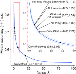
(a)

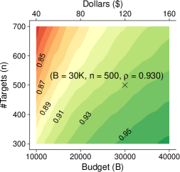
(b)

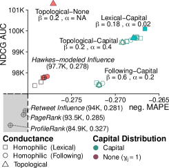
(c)

Figure 2. Evaluating GIM in three steps. (a) Select worker interface design features. The blue line shows the relation between the average accuracy (y-axis) and the noise ($\lambda$) (averaged over 100 simulations, $n=500$ targets, $B=30,000$). The points show ablations of design features (see Table 1) and their MLE fitted noise (relevant area zoomed in the inset). As more features are shown, worker accuracy increases. (b) Estimate required MTurk budget. We vary the number of targets ($n$, y-axis) and maximum budget ($B$, x-axis). The color map and contour annotations show the Spearman correlation between the BT-estimated influence raking ($\bm{\hat{\theta}}$) and a synthetic ground truth ($\bm{\theta}$). The cross denotes the chosen setup and estimated budget for our real-world experiments. (c) Evaluate GIM against the MTurk ground-truth in the space of NDCG-AUC (y-axis) and negative MAPE (x-axis). The solid shapes are the best models for each combination (conductance–capital distribution). The empty shapes show the Pareto-dominated models in each combination, obtained via grid search in the space $(\beta,\alpha)$. The circle-crosses denote the baselines: Hawkes-modeled influence baseline (Rizoiu et al., 2018), PageRank (Page et al., 1999), Retweet Influence (Cha et al., 2010), and ProfileRank (Silva et al., 2013). Note, the gray box is not to scale, and the coordinates for baselines are shown in brackets.

The homophilic conductance represents users through two lenses: following and lexical (see Section 3.1). For the following lens, we identify the $1000$ most followed users, and collect the followees of all the users in our dataset (i.e., users they follow). We represent a user $u_{i}$ as $h_{i}\in\mathbb{R}^{1000}$, where $h_{i}[j]=1$ if $u_{i}$ follows the $j$th most followed user ($h_{i}[j]=0$ otherwise). For the lexical lens, we construct user documents by concatenating the user tweets; we represent them using TF-IDF (Term Frequency-Inverse Document Frequency); and a feature hashing dimensionality reduction technique (Moody, 1989). Finally, we represent each user $u_{i}$ as $h_{i}\in\mathbb{R}^{1,048,576}$.

Evaluation metrics. We evaluate GIM ranking against the ground truth constructed in Section 4.2 using three measures: AUC-NDCG (see next), MAPE, and Spearman correlation. The information retrieval literature uses the Normalised Discounted Cumulative Gain (NDCG) to measure the overlap between two rankings. It privileges the correct ranking of the top-ranked positions and discounts errors in the lower rankings. Applied to influence, NDCG@k aims to order the $k$ most influential users correctly. We compute the Area Under Curve for NDCG@k (AUC-NDCG) by varying $k$ and producing a single metric value. We also compute the Mean Absolute Percentage Error (MAPE) of the difference in the ranking percentiles for each target.

MTurk worker study design. We account for three types of design features for the interface and the study: user features, proxies, and qualifications (shown in Table 1). The user features show information about each of the two targets, allowing the MTurk workers to assess them against each other quickly. We provide links to the online Twitter profile should the worker want to investigate. Proxy users are introduced to reduce the workers’ bias on their influence judgment—we ask workers who the proxy would find more influential. Proxies are selected similarly to targets (see Section 4.2). Finally, the qualifications are used to ban low-quality and ill-intentioned workers who randomly perform large amounts of comparisons, severely reducing worker accuracy. We describe in detail each of the design features, and we show the final worker interface in the online appendix (Appendix, 2021, Appendix C). Next, we perform a design feature ablation to show their relative importance for worker accuracy.

Table 1. Design features for the MTurk user study.

Feature name	Feature description
Username, picture & link	Twitter user profile information
Description	User-reported description
Tweet samples	Sample of 5 tweets emitted by the user
Follower Count	The number of people who follow the user
Followee Count	The number of people the user follows
Status Count	The number of posts the user has authored
Proxy User	A third user on whom the influence of each of the targets is projected
Qualifications	A mechanism to ban low-quality workers

4.2. Crowdsourced Influence Quantification

In this section, we build a user influence ground truth using the empirical influence measurement model introduced in Section 3.2.1.

Ablation study of worker interface features. We design the MTurk study iteratively, seeking to reduce the systematic noise (see Section 3.2.1). We perform an ablation study to add and remove design features, and measure worker accuracy against the follower count baseline. We run each ablation three times, and report the mean accuracy. Fig. 2(a) plots the relation between mean worker accuracy and the noise ($\lambda$), and places the outcomes of each ablation on this line. We make three observations. First, the user features provide a $15\%$ accuracy increase (from $0.57$ for no user features to $0.72$ for all features). The most important user features are follower count, followee count, and statuses count. Second, using proxies mitigates some worker bias ($3\%$ accuracy increase). Finally, removing the banning mechanism did not decrease the performance of the ablation study. This indicates that the low-quality workers did not show up for this experiment (probably discouraged by our prior banning). We henceforth use the complete set of features, which yields a worker accuracy of $0.72$ (corresponding to $\lambda=1.22$).

Estimate budget requirements. We use the determined noise parameter $\lambda=1.22$ and the simulation procedure introduced in Section 3.2.3 to determine the comparisons budget needed to achieve a suitably accurate influence ranking. We perform a grid search over the budget $B$ and the number of targets $n$, and show in Fig. 2(b) the obtained correlation between the influence ranking estimate and the synthetic ground truth. Visibly, the required budget increases with the number of targets, given a correlation level. In our experiment, we chose a correlation level of $0.93$ and $500$ targets, and estimate we require $30,000$ comparisons (approximately US$\$120$).

Build an influence ranking ground-truth. We select $500$ targets and $500$ proxies with available profiles (not suspended nor protected) who post in English—most MTurk workers come from English-speaking countries. We sample both high and low influence targets using the Hawkes-modeled influence baseline (Rizoiu et al., 2018) (full details of user sampling in the online appendix (Appendix, 2021, Appendix D)). We execute seven full quicksort runs, resulting in $36,252$ comparisons—slightly higher than our budget; still, we prefer to complete the final run. We obtain the ordered influence ranking of the $500$ targets. According to MTurk ethics and US Federal minimum wage, we paid MTurk workers US$\$0.04$ per task (10 pairwise comparisons).

4.3. GIM Evaluation

Here, we first find the best combination of conductance–distribution mechanism for GIM; we evaluate it against several baselines in influence estimation, including the current state-of-the-art Hawkes-modeled influence (Rizoiu et al., 2018); and we show it to be an unbiased alternative to the follower count metric.

Influence ranking baselines. We compare GIM to four baselines. Two baselines are widely used heuristics; PageRank (Page et al., 1999; Xiang et al., 2013) assumes influence flows via random-walks on constructed social graphs (here the follower network) and retweet influence (Cha et al., 2010), counts the retweets of a user’s authored tweets. They are centrality- and feature-based approaches, respectively. The other two baselines are purpose-built state-of-the-art influence estimators: Hawkes-modeled influence (Rizoiu et al., 2018) and ProfileRank (Silva et al., 2013) (a PageRank variant on Content-User bipartite network).

GIM search. For each combination of conductance (topological, lexical, and following) and distribution mechanism (social capital, and none), we perform a grid search over the hyper-parameters $\beta$ (conductance) and $\alpha$ (distribution). At each grid point we compare the influence scores obtained by GIM against the MTurk empirical influence ranking. Fig. 2(c) shows the baselines and GIM with several conductance-distribution combinations in the space of the performance measures: negative MAPE (x-axis) and NDCG-AUC (y-axis) (the top-right corner optimizes both measures).

We make three key observations. First, GIM consistently Pareto-dominates (i.e., outperforms) all baselines for almost every hyperparameter combinations, showing that our psychosocial-inspired mechanisms render automatic influence quantification closer to the human judgment. Among baselines, the best performing is the Hawkes-modeled influence, followed by PageRank, retweet influence, and the purpose-built ProfileRank. Second, we observe that the homophilic conductance typically outperforms the topological conductance and that the lexical outperforms the following conductance. Third, only two models are not Pareto-dominated: the topological-none (best NDCG-AUC) and the lexical-social capital (best neg. MAPE). Notice, however, that the topological conductance requires recovering the follower network. In practice, this is prohibitive for large datasets (such as the #Covid-19 dataset) due to rate limitations of the Twitter API. Therefore, in our analysis in Section 4.4 we use the homophilic lexical conductance ($\beta=0.18$) with the social capital distribution ($\alpha=0.02$). The $18\%$ baseline conductance indicates that the accounted channels do not explain a relatively large proportion of conductance. Note that while passing $2\%$ of the social capital to the parent might not seem much, this adds up for nodes with high degrees (particularly given the longtail distribution of follower count).

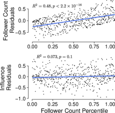
(a)

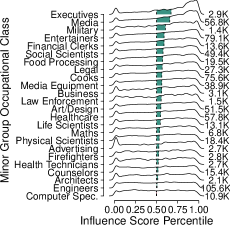
(b)

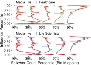
(c)

Figure 3. (a) Residuals (relative to the empirical follower ranking) for the follower count (top) and GIM (bottom) against the follower count (x-axis). (b) The influence distribution for the O*NET Minor Group occupations with more than 1,000 users in #Covid-19 (number of users shown on the right). Color bars show the difference between occupation mean influence and the general population (mean percentile influence of $0.5$). (c) Influence distribution (the dotted horizontal lines show means) tabulated into five bins according to users’ follower count; Media and Healthcare (top), and Media and Life Scientists (bottom)

Debiasing the follower count. The follower count is widely used as a proxy for influence (Cha et al., 2010; Frantz et al., 2009; Riddell et al., 2017); however, it has been repeatedly shown to be biased (Bakshy et al., 2011; Smith et al., 2018; Romero et al., 2011). Fig. 3(a)(top) shows that the follower count residuals—the difference between the follower count percentile and the empirical score percentile—are positively correlated with the follower count percentile ($R^{2}=0.48$). In other words, the follower count overestimates the influence of the highly followed users and underestimates the lowly followed users. Fig. 3(a) (bottom) shows that GIM residuals are not correlated with the follower count percentile ($R^{2}=0.073$). That is, GIM is an unbiased influence estimator with respect to the follower count.

4.4. Influence of Occupations during COVID

In this section, we first use GIM to compute the influence of all users in the #Covid-19 dataset. We tabulate their influence against their occupation and investigate the role of several occupations in pandemic-related discussions.

Determine the occupations of Twitter users. We match user occupation against the Minor Group Occupational Classes of the O*NET occupational taxonomy (for O*NET Development, [n.d.]) using textual fuzzy matching (Zhao et al., 2021). We search each user’s Twitter description and select the first matched occupation (following (Sloan et al., 2015))—assuming people list their actual occupation first, before hobbies or and other information.

The influence of occupations. Fig. 3(b) shows the distribution of influence scores for occupations with more than a thousand users in the #Covid-19 dataset. Executives, the Media, and the Military yield among the highest online influences. This result is hardly surprising for the former two. The latter is an occupation with high bipartisan support and respect in the US – home of most English-speaking Twitter users. Notably, Media and Entertainers are not only influential but have the most prominent online presences, perhaps on account of their attention-related business models. At the opposite end of the spectrum (and somewhat suprisingly) are Architects, Engineers and Computer Specialists with the lowest influence. Engineers, although prominent online, are not very influential and Computer Specialists have less influence than the general public.

Pandemic-related occupations. Next, we analyze the influence of three occupations heavily involved in communicating during the COVID-19 pandemic: Healthcare (including diagnosing and treating practitioners), Media and Communication, and Life Scientists. In Fig. 3(c), we compare pairs of these occupations tabulated against the follower count—influence’s most important covariate. We split the users into five equally-sized bins according to their follower count percentiles, and we plot influence distribution in each bin. We make three observations. First, the Media is more influential about the pandemic than the pandemic experts (Healthcare and Life Scientists), particularly in the highly-follower bins. While this is expected given the media’s role to inform the public, it could be problematic if the media outlets are more fringe and biased (Elejalde et al., 2018)) or cover misinformation and conspiracy theories. Second, the distributions in each bin show a mode around low influence scores. This reinforces prior findings that followership does not translate into large influence (Romero et al., 2011; Bakshy et al., 2011). Finally, Healthcare is more influential than Life Scientists, despite the latter including epidemiologists, medical scientists, and microbiologists; users are relying more on the advice of medical doctors and frontline workers than on research experts.

5. Related Work

Existing quantitative literature on influence measures are often limited to a narrow perspective of it. Common approaches include centrality measures (Cha et al., 2010; Francalanci and Hussain, 2017; Riddell et al., 2017; Asim et al., 2019), and influence maximization algorithms (Kempe et al., 2003; Agarwal and Mehta, 2020; Li et al., 2018); however, these often conflate influence with popularity and reach. Recent computational approaches (Qiu et al., 2018; Luceri et al., 2019, 2017) predict micro-level behavior but do not offer measures, and multivariate Hawkes approaches do not easily scale (Nickel and Le, 2021). Furthermore, crowdsourcing is commonly used to recover psychosocial attributes (Berinsky et al., 2012; Keith et al., 2017; Choi et al., 2020). Several recommender approaches utilize social concepts like homophily (Gulati and Eirinaki, 2019; Yu and Qin, 2019; Tsitsulin et al., 2018; Gu et al., 2018), and diffusions (Gulati and Eirinaki, 2019; Mukherjee and Günnemann, 2019). Arous et al. (2020) use crowdsourcing to find influencers, aggregating open-ended answers, but don’t provide an influence model capable of querying arbitrary users. To our knowledge, this is the first work to propose a Generalized Influence Model and tools to quantify it empirically.

6. Conclusion

Existing methods for online influence measurement rely on heuristic definitions and fail to model complex phenomena. In this work, we construct an online social influence pipeline. It includes an empirical measurement framework and GIM, accounting for socially informative channels (conductance) and attribution schemes (via distribution mechanisms). We estimate influence in discussions around the COVID-19 pandemic, finding that media, food processing, and even cooks are more influential than medical experts. Future work should include other influence signals beyond retweets and heterogeneous networks; it should incorporate assimilative and contrastive forms of influence.

Appendix

This document accompanies Conductance and Social Capital: Modeling and Empirically Measuring Online Social Influence, is presented for completeness, but is not required for understanding nor for reproducing its results.

Appendix A Complete derivation of GIM

This section shows the complete derivation from Eq. 3 to Eq. 5, both shown in the main text.

We define the influence of a tweet given the diffusion scenario $\mathcal{G}$, as:

(8) $$\varphi(v_{i}|\mathcal{G})=\sum_{v_{j}\in V(\mathcal{G})}\theta(i,j|\mathcal{G})$$

where $V(\mathcal{G})$ is the set of nodes in $\mathcal{G}$, and we denote as $\theta(i,j|\mathcal{G}):=\Psi(\mathcal{G}_{i\rightarrow j})$ the social capital distribution along a path. We start from the definition of GIM given a retweet cascade (main text Eq. 3):

$$\varphi_{\gamma}(v_{i}) =\mathbb{E}_{\mathcal{G}\in\Upsilon}\Big{[}\sum_{t_{j}>t_{i}}\mathds{1}(\mathcal{G}_{i\rightarrow j})\underbrace{\Psi(\mathcal{G}_{i\rightarrow j})}_{\text{Capital Distrib.}}\Big{]}$$

(9) $$=\sum_{\mathcal{G}\in\Upsilon}\mathbb{P}(\mathcal{G})\sum_{v_{j}\in V(\mathcal{G})}\theta(i,j|\mathcal{G})=\sum_{\mathcal{G}\in\Upsilon}\mathbb{P}(\mathcal{G})\varphi(v_{i}|\mathcal{G})$$

Notably, due to the factorial number of diffusion scenarios in $\Upsilon$, computing the influence for each graph is intractable. For example, there are $10^{156}$ diffusion scenarios for a cascade of 100 retweet (Rizoiu et al., 2018).

Incremental construction of diffusion scenarios. We leverage the independent cascades assumption (see main text Section 2.1) to construct an efficient influence computation that overcomes intractablility. The key observation is that each tweet $v_{k}$ is added simultaneously at time $t_{k}$ to all diffusion scenarios constructed at time $t_{k-1}$. $v_{k}$ contributes only once to the tweet influence of every tweet found on the path to which $v_{k}$ is attached. The tweet influence is computed incrementally by updating $\varphi(v_{i}),i<k$ at each time $t_{k}$. We denote by $\varphi^{k}(v_{i})$ the value of tweet influence of $v_{i}$ after adding node $v_{k}$. As a result, we only track how the tweet influence increases over time steps, and we do not construct all valid diffusion scenarios.

GIM assumes that a user’s tweet is influenced by one of the precedent tweets, chosen stochastically from a discrete distribution over the valid edges. Alternatively, we can interpret that all previous tweets influence the new tweet proportionally to the same discrete distribution (a view inline with recent findings about influence and complex contagion). Let $\Upsilon_{1:k-1}$ be the set of all possible diffusion scenarios at time $t_{k-1}$, and $\mathcal{G}^{-}\in\Upsilon_{1:k-1}$ be one such diffusion scenario, with the set of nodes $V^{-}=\{v_{1},v_{2},\cdots,v_{k-1}\}$. When $v_{k}$ arrives, it can attach to any node in $V^{-}$, generating $k-1$ new diffusion scenarios $\mathcal{G}_{j}^{+}$, with $V_{j}^{+}=V^{-}\cup v_{k}$ and $E_{j}^{+}=E^{-}\cup(v_{j},v_{k})$. We can write the set of scenarios at time $t_{k}$ as:

(10) $$\Upsilon_{1:k}=\left\{\mathcal{G}_{j}^{+}\middle|\forall j<k,\forall\mathcal{G}^{-}\in\Upsilon_{1:k-1}\right\}$$

We write the tweet influence of $v_{i}$ at time $k$ as:

$$\varphi^{k}(v_{i})=\sum_{\mathcal{G}^{+}\in\Upsilon_{1:k}}\mathds{P}(\mathcal{G}^{+})\varphi(v_{i}|\mathcal{G}^{+})\\$$

(11) $${}^{cf.~{}\eqref{eq:diff-scenario-increase}} =\sum_{\mathcal{G}^{-}\in\Upsilon_{1:k-1}}\sum^{k-1}_{j=1}\mathds{P}(\mathcal{G}_{j}^{+})\varphi(v_{i}|\mathcal{G}_{j}^{+})$$

Attach a new node $v_{k}$. We concentrate on the right-most factor in Eq. (11) – the tweet influence in scenario $\mathcal{G}^{+}_{j}$. We observe that the terms in Eq. (8) divide into two: the paths from $v_{i}$ to all other nodes except $v_{k}$ (i.e. the old nodes) and the path from $v_{i}$ to $v_{k}$. We obtain:

$$\varphi(v_{i}|\mathcal{G}_{j}^{+})=\sum_{\begin{subarray}{c}v_{l}\in{\mathcal{G}_{j}^{+}}\\ l>i,l\neq k\end{subarray}}\theta(i,l|\mathcal{G}_{j}^{+})+\theta(i,k|\mathcal{G}_{j}^{+})$$

Note that a path that does not involve $v_{k}$ has the same influence capital contribution in $\mathcal{G}_{j}^{+}$ and in its parent scenario $\mathcal{G}^{-}$, i.e. $\theta(i,l|\mathcal{G}_{j}^{+})=\theta(i,l|\mathcal{G}^{-}),\text{ for }l>i,\text{and }l\neq k$. We obtain

$$\varphi(v_{i}|\mathcal{G}_{j}^{+}) =\sum_{\begin{subarray}{c}v_{l}\in{\mathcal{G}^{-}}\\ l>i\end{subarray}}\theta(i,l|\mathcal{G}^{-})+\theta(i,k|\mathcal{G}_{j}^{+})$$

(12) $${}^{cf.~{}\eqref{eq:infl-in-a-scenario}} =\varphi(v_{i}|\mathcal{G}^{-})+\theta(i,k|\mathcal{G}_{j}^{+})$$

Combining Eq. (11) and (12), we obtain:

$$\varphi^{k}(v_{i})=\sum_{\mathcal{G}^{-}\in\Upsilon_{1:k-1}}\sum^{k-1}_{j=1}\mathds{P}(\mathcal{G}_{j}^{+})\bigg{[}\varphi(v_{i}|\mathcal{G}^{-})+\theta(i,k|\mathcal{G}_{j}^{+})\bigg{]}$$

(13) $$=\underbrace{\sum_{\mathcal{G}^{-}\in\Upsilon_{1:k-1}}\varphi(v_{i}|\mathcal{G}^{-})\sum^{k-1}_{j=1}\mathds{P}(\mathcal{G}_{j}^{+})}_{A}+\underbrace{\sum_{\mathcal{G}^{-}\in\Upsilon_{1:k-1}}\sum^{k-1}_{j=1}\mathds{P}(\mathcal{G}_{j}^{+})\theta(i,k|\mathcal{G}_{j}^{+})}_{m_{ik}}$$

Tweet influence at previous time step $t_{k-1}$. Given the definition of $\mathcal{G}_{j}^{+}$ in Eq. 10 and the independant cascades assumption, we obtain that $\mathds{P}(\mathcal{G}_{j}^{+})=\mathds{P}(\mathcal{G}^{-})p^{\prime}_{ij}$. Consequently, part $A$ in Eq. 13 can be written as:

$$A =\sum_{\mathcal{G}^{-}\in\Upsilon_{1:k-1}}\varphi(v_{i}|\mathcal{G}^{-})\sum^{k-1}_{j=1}\mathds{P}(\mathcal{G}^{-})p^{\prime}_{jk}$$

(14) $$=\sum_{\mathcal{G}^{-}\in\Upsilon_{1:k-1}}\varphi(v_{i}|\mathcal{G}^{-})\mathds{P}(\mathcal{G}^{-})\sum^{k-1}_{j=1}p^{\prime}_{jk}\stackrel{{\scriptstyle{cf.~{}\eqref{eq:brute-user-infl}}}}{{=}}\varphi^{k-1}(v_{i})$$

$A$ is the tweet influence of $v_{i}$ at the previous time step $t_{k-1}$. Note that $\sum^{k-1}_{j=1}p^{\prime}_{jk}=1$ because $v_{k}$ is necessarily the direct retweet of a previous nodes $v_{j},j<k$ of the retweet cascade.

Contribution of $v_{k}$. With $A$ being the influence of $v_{i}$ at the previous time step, intuitively $m_{ik}$ is the contribution of $v_{k}$ to the influence of $v_{i}$. Knowing that:

$$\mathds{P}(\mathcal{G}_{j}^{+}) =\mathds{P}(\mathcal{G}^{-})p^{\prime}_{jk}\text{ and }$$

$$\theta(i,k|\mathcal{G}_{j}^{+}) =\Psi(\mathcal{\mathcal{G}}_{i\rightarrow j})\pi_{jk}\ ^{cf.\ref{eq:capital-distrib-path}}$$

$$=\theta(i,j|\mathcal{G}^{+}_{j})\pi_{jk}$$

$$=\theta(i,j|\mathcal{G}^{-})\pi_{jk}$$

we write $m_{ik}$ as:

$$m_{ik} =\sum_{\mathcal{G}^{-}\in\Upsilon_{1:k-1}}\sum^{k-1}_{j=1}\mathds{P}(\mathcal{G}^{-})p^{\prime}_{jk}\theta(i,j|\mathcal{G}^{-})\pi_{jk}$$

$$=\sum^{k-1}_{j=1}p^{\prime}_{jk}\pi_{jk}\underbrace{\sum_{\mathcal{G}^{-}\in\Upsilon_{1:k-1}}\mathds{P}(\mathcal{G}^{-})\theta(i,j|\mathcal{G}^{-})}_{m_{ij}}=\sum^{k-1}_{j=1}p^{\prime}_{jk}\pi_{jk}m_{ij}\ ^{cf.\ref{eq:gim-mik}}$$

Appendix B Efficient computation of GIM

We define two matrices. First, the transfer matrix $T=[p^{\prime}_{ij}*\pi_{ij}]$, where the element $p^{\prime}_{ij}$ is the probability that tweet $v_{j}$ is a direct retweet of tweet $v_{i}$ (defined in Eq. 4) and $\pi_{ij}$ is the proportion of capital transfered from $v_{j}$ to $v_{i}$; Second, the influence accumulation matrix $M=[m_{ij}]$, with $m_{ij}$ defined in Eq. (5) is the contribution of $v_{j}$ to the influence of $v_{i}$. For each column $j$ of $M$, we compute the first $j-1$ elements by multiplying the sub-matrix $M_{[1..j-1,1..j-1]}$ with the first $j-1$ elements on the $j^{th}$ column of matrix $T$, the $j$-th element is $\pi_{jj}$, and the remaining elements are $0$. The computation of matrix $M$ finishes after $n$ steps, where $n$ is the total number of retweets in the cascade.

Appendix C MTurk Interface & Systematic Noise

In this section, we briefly describe the generic setup and design interventions utilized to reduce systematic noise. Here we illustrate several of the design features (summarised in Table 1), including the user component, proxies, and qualifications. We assess the design features via an ablation study, and fit the noise associated with particular feature sets (see Section 3.2.3), shown in Fig. 2(a).

Generic setup. We utilize the ubiquitous MTurk crowdsourcing platform to implement the quicksort active learning procedure. The implementation runs quicksort partitions concurrently, such that comparison pairs enter a FIFO queue and are served to MTurk workers in batches of $10$. Each global quicksort procedure over the entire sample called a run, is executed sequentially such that no identical pairs are shown in the same batch since quicksort compares items at most once. The workers were presented with two target users and a proxy user (see below). Workers were asked, via a pool of differently worded questions, to determine which target user was more influential to the proxy. These questions are “Which user is the proxy user most likely to retweet?”, “Who will the proxy user be more socially influenced by?”, and “Which user would sway the proxy users opinion more?”. We performed three runs for each ablation and removed the banning of workers between ablations.

The user component was designed so workers could quickly glean the relevant information about users, with the users’ names, pictures, descriptions, hyperlinks to their Twitter profile, and a small sample of their tweets presented. Additionally, the component included various user metrics, including the follower count, followee count, and statuses count. Fig. 2(a) shows the removal of these metrics significantly reduces the accuracy. When all metrics are removed, we observe the worst decision accuracy $0.57$. In particular, when only the followee or status metrics are present, we observe an increased accuracy of $0.61$ and $0.68$, respectively; when both are present (without follower count), we observe another accuracy increase to $0.70$. Note that when all metrics are included, the accuracy increases to $0.72$, which cumulatively suggests that all metrics are independently important signals of influence; however, there is some mutual information between the metrics.

Proxy users are used to reduce the effect of a worker’s opinion on their influence judgment. In judging between two targets, a worker is asked who the proxy finds more influential. Proxy users do not eliminate the workers’ subjectivity; however, they might mitigate some noise introduced in this area. Removing the feature noticeably reduces the decision accuracy to $0.69$.

The qualification system restricts designated workers from completing tasks. A common phenomenon on MTurk is that workers accept many tasks of the same type concurrently (and effectively reserve those tasks for future completion), allowing workers to complete large proportions of the work. The responses of some workers might be consistently inaccurate for several reasons; they are answering randomly for monetary gain, they do not understand the task or social context, or they respond in bad faith for some other reason. We broadly label such workers as low-quality workers. If low-quality workers complete large proportions of work, reducing overall quality, and accordingly, we ban them dynamically.

We measure the quality of a worker, within a run, as the accuracy of the workers’ responses concerning the follower count percentiles of targets. As the task is inherently subjective and difficult, we add some leniency to this banning scheme. Firstly, only comparisons where the difference of follower count percentiles is greater than $0.2$ are included in determining accuracy. The intuition is that targets with quasi-equivalent influence are difficult to judge. Secondly, banning is only implemented after having completed $100$ comparisons that satisfy the prior condition. Lastly, the banning decision is only made once per run (but a banned worker is banned forever). This banning scheme is lenient enough that work is completed quickly, while restrictive enough that response quality remains high. Removing the intra-banning mechanism performs slightly better than the baseline, with an accuracy of $0.73$, which might be explained by ‘low-quality workers’ being discouraged from that task by previous interactions with the experiment. For this reason, we use the full feature set for the final experiment.

Appendix D Target and proxy sample selection.

We selected from the #ArsonEmergency dataset a sample of $500$ targets and $500$ proxies, controlled for availability, language, and Hawkes-modeled influence. The users’ availability (suspended or protected status at the time of the experiment) was queried through the Twitter API before the experiment. To determine if a user was English-speaking (so the majoritively English-speaking MTurk workers could appropriately judge them), triple-agreement was used between three language detection systems langid (Lui and Baldwin, 2012), cld3 (Google, [n.d.]), and whatthelang. We verified the (55.8% remaining) filtered users were uniform with respect to Hawkes-modeled influence, via a chi-square test at a 95% significance level. From this set of valid users, we used an inverse CDF sampling method, with nearest-matching, to sample users with respect to Hawkes-modeled influence.

References

- (1)
- Agarwal and Mehta (2020) Sakshi Agarwal and Shikha Mehta. 2020. Effective influence estimation in twitter using temporal, profile, structural and interaction characteristics. Information Processing & Management 57, 6 (2020), 102321.
- Ailon (2008) Nir Ailon. 2008. Reconciling real scores with binary comparisons: A new logistic based model for ranking. Advances in Neural Information Processing Systems (2008).
- Appendix (2021) Online Appendix. 2021. Appendix: Conductance and Social Capital: Modeling and Empirically Measuring Online Social Influence. https://www.dropbox.com/s/963oc5fx4f7412p/Supplementary_Material.pdf?dl=0.
- Arous et al. (2020) Ines Arous, Jie Yang, Mourad Khayati, and Philippe Cudré-Mauroux. 2020. Opencrowd: A human-ai collaborative approach for finding social influencers via open-ended answers aggregation. In Proceedings of The Web Conference 2020. 1851–1862.
- Asch (1961) Solomon E Asch. 1961. Effects of group pressure upon the modification and distortion of judgments. In Documents of gestalt psychology. University of California Press, 222–236.
- Asim et al. (2019) Yousra Asim, Ahmad Kamran Malik, Basit Raza, and Ahmad Raza Shahid. 2019. A trust model for analysis of trust, influence and their relationship in social network communities. Telematics and Informatics 36 (2019), 94–116.
- Bakshy et al. (2011) Eytan Bakshy, Jake M Hofman, Winter A Mason, and Duncan J Watts. 2011. Everyone’s an influencer: quantifying influence on twitter. In Proceedings of the fourth ACM international conference on Web search and data mining. 65–74.
- Berinsky et al. (2012) Adam J Berinsky, Gregory A Huber, and Gabriel S Lenz. 2012. Evaluating online labor markets for experimental research: Amazon. com’s Mechanical Turk. Political analysis 20, 3 (2012), 351–368.
- Bikhchandani et al. (1992) Sushil Bikhchandani, David Hirshleifer, and Ivo Welch. 1992. A theory of fads, fashion, custom, and cultural change as informational cascades. Journal of political Economy 100, 5 (1992), 992–1026.
- Bradley and Terry (1952) Ralph Allan Bradley and Milton E Terry. 1952. Rank analysis of incomplete block designs: I. The method of paired comparisons. Biometrika (1952).
- Buhrmester et al. (2016) Michael Buhrmester, Tracy Kwang, and Samuel D Gosling. 2016. Amazon’s Mechanical Turk: A new source of inexpensive, yet high-quality data? (2016).
- Cattelan (2012) Manuela Cattelan. 2012. Models for paired comparison data: A review with emphasis on dependent data. Statist. Sci. (2012).
- Cattelan et al. (2013) Manuela Cattelan, Cristiano Varin, and David Firth. 2013. Dynamic Bradley–Terry modelling of sports tournaments. Journal of the Royal Statistical Society: Series C (Applied Statistics) 62, 1 (2013), 135–150.
- Cha et al. (2010) Meeyoung Cha, Hamed Haddadi, Fabricio Benevenuto, and Krishna Gummadi. 2010. Measuring user influence in twitter: The million follower fallacy. In Proceedings of the international AAAI conference on web and social media, Vol. 4.
- Choi et al. (2020) Minje Choi, Luca Maria Aiello, Krisztián Zsolt Varga, and Daniele Quercia. 2020. Ten social dimensions of conversations and relationships. In Proceedings of The Web Conference 2020. 1514–1525.
- Cialdini (2001) Robert B Cialdini. 2001. Influence: Science and practice.
- Crandall et al. (2008) David Crandall, Dan Cosley, Daniel Huttenlocher, Jon Kleinberg, and Siddharth Suri. 2008. Feedback effects between similarity and social influence in online communities. In Knowledge Discovery and Data Mining (KDD’08). 160–168.
- Du et al. (2013a) Nan Du, Le Song, Manuel Gomez-Rodriguez, and Hongyuan Zha. 2013a. Scalable influence estimation in continuous-time diffusion networks. NIPS (2013).
- Du et al. (2013b) Nan Du, Le Song, Manuel Gomez-Rodriguez, and Hongyuan Zha. 2013b. Scalable influence estimation in continuous-time diffusion networks. In Advances in Neural Information Processing Systems (NIPS), Vol. 26. NIH Public Access, 3147.
- Elejalde et al. (2018) Erick Elejalde, Leo Ferres, and Eelco Herder. 2018. On the nature of real and perceived bias in the mainstream media. PloS one 13, 3 (2018), e0193765.
- for O*NET Development ([n.d.]) National Center for O*NET Development. [n.d.]. O*NET OnLine,. https://www.onetonline.org/. Accessed: 2021-06-30.
- Francalanci and Hussain (2017) Chiara Francalanci and Ajaz Hussain. 2017. Influence-based Twitter browsing with NavigTweet. Information Systems 64 (2017), 119–131.
- Frantz et al. (2009) Terrill L Frantz, Marcelo Cataldo, and Kathleen M Carley. 2009. Robustness of centrality measures under uncertainty: Examining the role of network topology. Computational and Mathematical Organization Theory 15, 4 (2009), 303–328.
- Goel et al. (2016) Rahul Goel, Sandeep Soni, Naman Goyal, John Paparrizos, Hanna Wallach, Fernando Diaz, and Jacob Eisenstein. 2016. The social dynamics of language change in online networks. In International conference on social informatics. Springer, 41–57.
- Google ([n.d.]) Google. [n.d.]. CLD3. https://github.com/google/cld3
- Graham and Keller (2020) T Graham and TR Keller. 2020. Bushfires, bots and arson claims: Australia flung in the global disinformation spotlight. The Conversation 10 (2020).
- Gu et al. (2018) Yupeng Gu, Yizhou Sun, Yanen Li, and Yang Yang. 2018. Rare: Social rank regulated large-scale network embedding. In Proceedings of the 2018 World Wide Web Conference. 359–368.
- Gulati and Eirinaki (2019) Avni Gulati and Magdalini Eirinaki. 2019. With a little help from my friends (and their friends): Influence neighborhoods for social recommendations. In The World Wide Web Conference. 2778–2784.
- Hawkes (1971) Alan G Hawkes. 1971. Spectra of some self-exciting and mutually exciting point processes. Biometrika (1971).
- Hawkes and Oakes (1974) Alan G Hawkes and David Oakes. 1974. A cluster process representation of a self-exciting process. Journal of Applied Probability (1974).
- Hoare (1962) Charles AR Hoare. 1962. Quicksort. Comput. J. (1962).
- Horai et al. (1974) Joann Horai, Nicholas Naccari, and Elliot Fatoullah. 1974. The effects of expertise and physical attractiveness upon opinion agreement and liking. Sociometry (1974), 601–606.
- Keith et al. (2017) Melissa G Keith, Louis Tay, and Peter D Harms. 2017. Systems perspective of Amazon Mechanical Turk for organizational research: Review and recommendations. Frontiers in psychology 8 (2017), 1359.
- Kempe et al. (2003) David Kempe, Jon Kleinberg, and Éva Tardos. 2003. Maximizing the spread of influence through a social network. In Proceedings of the ninth ACM SIGKDD international conference on Knowledge discovery and data mining. 137–146.
- Kruis and Borsboom (2020) Joost Kruis and Denny Borsboom. 2020. Patrick Mair: Modern Psychometrics with R.
- Lenton (2006) Richard Lenton. 2006. Using the method of paired comparisons in non-designed experiments. Ph.D. Dissertation. Griffith University.
- Lewis and Mohler (2011) Erik Lewis and George Mohler. 2011. A nonparametric EM algorithm for multiscale Hawkes processes. Journal of Nonparametric Statistics (2011).
- Li et al. (2018) Yuchen Li, Ju Fan, Yanhao Wang, and Kian-Lee Tan. 2018. Influence maximization on social graphs: A survey. IEEE Transactions on Knowledge and Data Engineering 30, 10 (2018), 1852–1872.
- Lin et al. (2018) Lynda C Lin, Yang Qu, and Eva H Telzer. 2018. Intergroup social influence on emotion processing in the brain. Proceedings of the National Academy of Sciences 115, 42 (2018), 10630–10635.
- Luceri et al. (2019) Luca Luceri, Torsten Braun, and Silvia Giordano. 2019. Analyzing and inferring human real-life behavior through online social networks with social influence deep learning. Applied network science 4, 1 (2019), 1–25.
- Luceri et al. (2017) Luca Luceri, Alberto Vancheri, Torsten Braun, and Silvia Giordano. 2017. On the social influence in human behavior: Physical, homophily, and social communities. In International Conference on Complex Networks and their Applications. Springer, 856–868.
- Lui and Baldwin (2012) Marco Lui and Timothy Baldwin. 2012. langid. py: An off-the-shelf language identification tool. In Proceedings of the ACL 2012 system demonstrations.
- Mason et al. (2007) Winter A Mason, Frederica R Conrey, and Eliot R Smith. 2007. Situating social influence processes: Dynamic, multidirectional flows of influence within social networks. Personality and social psychology review 11, 3 (2007), 279–300.
- Maystre and Grossglauser (2017) Lucas Maystre and Matthias Grossglauser. 2017. Just sort it! A simple and effective approach to active preference learning. In International Conference on Machine Learning.
- Milgram and Gudehus (1978) Stanley Milgram and Christian Gudehus. 1978. Obedience to authority.
- Mishra et al. (2016) Swapnil Mishra, Marian-Andrei Rizoiu, and Lexing Xie. 2016. Feature driven and point process approaches for popularity prediction. In Proceedings of the 25th ACM international on conference on information and knowledge management. 1069–1078.
- Moody (1989) John Moody. 1989. Fast learning in multi-resolution hierarchies. In Advances in neural information processing systems. 29–39.
- Mukherjee and Günnemann (2019) Subhabrata Mukherjee and Stephan Günnemann. 2019. GhostLink: Latent Network Inference for Influence-aware Recommendation. In The World Wide Web Conference. 1310–1320.
- Newcomb (1953) Theodore M Newcomb. 1953. An approach to the study of communicative acts. Psychological review 60, 6 (1953), 393.
- Nickel and Le (2021) Maximilian Nickel and Matthew Le. 2021. Modeling Sparse Information Diffusion at Scale via Lazy Multivariate Hawkes Processes. In Proceedings of the Web Conference 2021. 706–717.
- Nowak et al. (2005) Andrzej Nowak, Robin R Vallacher, Marek Kus, and Jakub Urbaniak. 2005. The dynamics of societal transition: Modeling nonlinear change in the Polish economic system. International Journal of Sociology 35, 1 (2005), 65–88.
- Page et al. (1999) Lawrence Page, Sergey Brin, Rajeev Motwani, and Terry Winograd. 1999. The PageRank citation ranking: Bringing order to the web. Technical Report. Stanford InfoLab.
- Peng et al. (2018) Sancheng Peng, Yongmei Zhou, Lihong Cao, Shui Yu, Jianwei Niu, and Weijia Jia. 2018. Influence analysis in social networks: A survey. Journal of Network and Computer Applications 106 (2018), 17–32.
- Qiu et al. (2018) Jiezhong Qiu, Jian Tang, Hao Ma, Yuxiao Dong, Kuansan Wang, and Jie Tang. 2018. Deepinf: Social influence prediction with deep learning. In Proceedings of the 24th ACM SIGKDD International Conference on Knowledge Discovery & Data Mining. 2110–2119.
- Riddell et al. (2017) Jeff Riddell, Alisha Brown, Ivor Kovic, and Joshua Jauregui. 2017. Who are the most influential emergency physicians on Twitter? Western Journal of Emergency Medicine 18, 2 (2017), 281.
- Rizoiu et al. (2018) Marian-Andrei Rizoiu, Timothy Graham, Rui Zhang, Yifei Zhang, Robert Ackland, and Lexing Xie. 2018. # debatenight: The role and influence of socialbots on twitter during the 1st 2016 us presidential debate. In AAAI.
- Romero et al. (2011) Daniel M Romero, Wojciech Galuba, Sitaram Asur, and Bernardo A Huberman. 2011. Influence and passivity in social media. In Joint European Conference on Machine Learning and Knowledge Discovery in Databases. Springer, 18–33.
- Settles (2009) Burr Settles. 2009. Active learning literature survey. (2009).
- Shah et al. (2016) Nihar B Shah, Sivaraman Balakrishnan, Joseph Bradley, Abhay Parekh, Kannan Ramchandran, and Martin J Wainwright. 2016. Estimation from pairwise comparisons: Sharp minimax bounds with topology dependence. The Journal of Machine Learning Research (2016).
- Silva et al. (2013) Arlei Silva, Sara Guimarães, Wagner Meira Jr, and Mohammed Zaki. 2013. ProfileRank: finding relevant content and influential users based on information diffusion. In Proceedings of the 7th Workshop on Social Network Mining and Analysis. 1–9.
- Sloan et al. (2015) Luke Sloan, Jeffrey Morgan, Pete Burnap, and Matthew Williams. 2015. Who tweets? Deriving the demographic characteristics of age, occupation and social class from Twitter user meta-data. PloS one 10, 3 (2015), e0115545.
- Smith et al. (2018) Steven T Smith, Edward K Kao, Danelle C Shah, Olga Simek, and Donald B Rubin. 2018. Influence estimation on social media networks using causal inference. In 2018 IEEE Statistical Signal Processing Workshop (SSP). IEEE, 328–332.
- Tsitsulin et al. (2018) Anton Tsitsulin, Davide Mottin, Panagiotis Karras, and Emmanuel Müller. 2018. Verse: Versatile graph embeddings from similarity measures. In Proceedings of the 2018 World Wide Web Conference. 539–548.
- Tsukida and Gupta (2011) Kristi Tsukida and Maya R Gupta. 2011. How to analyze paired comparison data. Technical Report. WASHINGTON UNIV SEATTLE DEPT OF ELECTRICAL ENGINEERING.
- Xiang et al. (2013) Biao Xiang, Qi Liu, Enhong Chen, Hui Xiong, Yi Zheng, and Yu Yang. 2013. Pagerank with priors: An influence propagation perspective. In Twenty-Third International Joint Conference on Artificial Intelligence.
- Yu and Qin (2019) Wenhui Yu and Zheng Qin. 2019. Spectrum-enhanced pairwise learning to rank. In The World Wide Web Conference. 2247–2257.
- Zermelo (1929) Ernst Zermelo. 1929. Die berechnung der turnier-ergebnisse als ein maximumproblem der wahrscheinlichkeitsrechnung. Mathematische Zeitschrift (1929).
- Zhao et al. (2021) Yi Zhao, Haixu Xi, and Chengzhi Zhang. 2021. Exploring Occupation Differences in Reactions to COVID-19 Pandemic on Twitter. Data and Information Management 5, 1 (2021), 110–118.