Multipartitioning topological phases by vertex states and quantum entanglement

Abstract

We discuss multipartitions of the gapped ground states of (2+1)-dimensional topological liquids into three (or more) spatial regions that are adjacent to each other and meet at points. By considering the reduced density matrix obtained by tracing over a subset of the regions, we compute various correlation measures, such as entanglement negativity, reflected entropy, and associated spectra. We utilize the bulk-boundary correspondence to show that such multipartitions can be achieved by using what we call vertex states in (1+1)-dimensional conformal field theory – these are a type of state used to define an interaction vertex in string field theory and can be thought of as a proper generalization of conformal boundary states. This approach allows an explicit construction of the reduced density matrix near the entangling boundaries. We find the fingerprints of topological liquid in these quantities, such as (universal pieces in) the scaling of the entanglement negativity, and a non-trivial distribution of the spectrum of the partially transposed density matrix. For reflected entropy, we test the recent claim that states the difference between reflected entropy and mutual information is given, once short-range correlations are properly removed, by $(c/3)\ln 2$ where $c$ is the central charge of the topological liquid that measures ungappable edge degrees of freedom. As specific examples, we consider topological chiral $p$-wave superconductors and Chern insulators. We also study a specific lattice fermion model realizing Chern insulator phases and calculate the correlation measures numerically, both in its gapped phases and at critical points separating them.

I Introduction

“Quantum entanglement is not one but the characteristic trait of quantum mechanics, the one that enforces its entire departure from classical lines of thought” schrodinger_1935 . Entanglement also plays a central role in understanding various phenomena and phases in many-body quantum physics. For example, the scaling of the entanglement entropy defined for a given subregion is a useful probe to understand different phases of matter and renormalization group flows connecting them 2003PhRvL..90v7902V ; 2009JPhA…42X4005C ; levin2006detecting ; kitaev2006topological ; 2007JSMTE..08…24H ; 2007JPhA…40.7031C ; 2018RvMP…90c5007N . Modern approaches to many-body quantum problems, such as the density matrix renormalization group and tensor networks, are based on the concept of quantum entanglement Fradkin:2013sab ; 2013NJPh…15b5002G ; LAFLORENCIE20161 ; zeng2018quantum ; Verstraete_2008 .

Quantum entanglement is particularly useful for characterizing topological phases of matter, which lack conventional order parameters. One of the simplest settings to consider is a bipartition of the ground state of a topological liquid into two spatial subregions, $A$ and its complement $\bar{A}$, say. We can then study the scaling of the entanglement entropy as a function of the size of the subregion $A$, which allows us to extract the topological entanglement entropy of the topologically ordered ground state levin2006detecting ; kitaev2006topological . One can also study the entanglement spectrum, which also serves as a probe of different topological orders and symmetry-protected topological phases Ryu_2006 ; PhysRevLett.101.010504 ; Pollmann_2010 .

In this paper, we move beyond bipartitions and consider multipartitions of the ground states of (2+1)-dimensional topological liquids. Specifically, we consider a tripartition (multipartition) in which the boundaries between the three subregions $A$, $B$, and $C$ meet at a junction, as shown in Fig. 1. We note that this partitioning is analogous to the one first considered in Ref. kitaev2006topological . A similar setup was also used recently in 2021arXiv211006932K ; kim2021modular to derive a formula for the chiral central charge in terms of the modular commutator.

This multipartition setting allows us to define and compute various correlation measures. For example, when one of the three subregions, say $C$, is traced out, we are left with the reduced density matrix for $A\cup B$, which is now mixed. We can then discuss mixed state correlation measures, such as the entanglement negativity Zyczkowski:1998yd ; Vidal:2002zz ; Peres:1996dw ; 1999JMOp…46..145E ; 2005PhRvL..95i0503P ; 2000PhRvL..84.2726S ; 1996PhLA..223….1H and reflected entropy dutta2021canonical . We can also study the associated spectra, such as the spectrum of the partially transposed density matrix. These entanglement measures may capture universal data related to multipartite entanglement of topologically-ordered ground states, which are not accessible in bipartition settings. (For previous studies on multipartite correlations in topological liquid, see, for example, 2016PhRvA..93b2317K .)

The entanglement negativity and reflected entropy have been previously studied in the context of topologically-ordered phases in setups different from ours 2013PhRvA..88d2318L ; castelnovo2013negativity ; wen2016edge ; wen2016surgery ; lim2021disentangling ; berthiere2021 . We give a brief overview of the previous results in Sec. II. As for the reflected entropy, for the tripartition setup above, it was recently claimed BerkeleyPaper that the difference between the reflected entropy and mutual information is given by $(c/3)\ln 2+{\cal O}(e^{-\ell/\xi})$ where $c$ is the central charge of the topological liquid, $\xi$ is the correlation length and $\ell$ is the length scale for the three regions. (To obtain the above universal value non-universal short-range correlations must be removed by a proper local unitary – see Sec. II.) As this multiparty entanglement quantity may capture the central charge, the vanishing of this quantity may be a prerequisite of having a PEPS (projected entangled pair state) representation of the topological liquid with finite bond dimension. (Or non-vanishing of this quantity may be an obstruction to having a PEPS representation with finite bond dimension.) We will review this claim in Sec. II. These observations suggest that there is much yet to be understood regarding topological phases from the lens of entanglement.

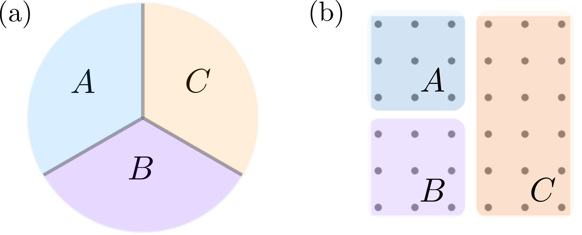
Figure 1: Tripartition of topological liquid on a two-dimensional plane (a) and two-dimensional square lattice (b).

We study the tripartition of topological phases using two different approaches. First, we employ the edge theory or “cut-and-glue” approach for computing the entanglement of topological phases qi2012general ; lundgren2013cutandglue ; cano2015interfaces ; wen2016edge ; sohal2020nonabelian , in which one approximates the entanglement between the bulk regions as arising purely from entanglement of the gapped chiral edge modes along the entanglement cuts between the bulk regions. This approach is not limited to non-interacting phases (e.g. integer quantum Hall or Chern insulator phases) but rather is also applicable to generic topologically-ordered phases. We recall that for the case of bipartitioning a topological liquid, the entanglement entropy (and other related quantities) can be obtained from conformal boundary states (Ishibashi states) qi2012general ; wen2016edge ; wong2018note ; fliss2017interface . (See Sec. III.1.1.) In this work, we will extend this approach to the case of a multipartition (tripartition) by considering what we call “vertex states,” which will be introduced in Sec. III.1. What the vertex states do for the case of tripartitioning is quite analogous to what Ishibashi states do for the case of bipartitioning. We emphasize that the construction of these vertex states is a nontrivial extension of the corresponding computation for a bipartition, even for the case of free fermions. Indeed, with some minor differences, states similar to vertex states have been considered in the context of string field theory gross1987field ; gross1987operator ; gross1987operator2 ; leclair1989string . They also resemble open boundary states or rectangular states in conformal field theory imamura2006boundary ; imamura2008boundary ; bondesan2012conformal ; bondesan2013rectangular . We will construct these vertex states using two methods: the Neumann coefficient method, which makes use of conformal mappings to fix the form of the vertex state, and a direct calculation method, in which we directly diagonalize the boundary conditions defining the vertex state. We check their equivalence numerically.

In the second approach, we consider the tripartite entanglement of a specific non-interacting lattice fermion model that realizes a Chern insulator phase. The many-body ground state is given by a Gaussian state (namely, a Slater determinant state), which allows us to make use of the “correlator method” developed in Refs. peschel2003calculation ; chung2001density to compute various correlation measures. In contrast to the edge theory calculation, which is only applicable for a system deep in the topological phase, here we can study how the correlation measures of interest change as we tune across the phase transition between the topological and trivial phases.

This paper is organized as follows. In Sec. II, we introduce the correlation measures of interest and the correlator method. In Subsec. III.1, after reviewing the edge theory approach to computing entanglement in bipartition settings, we introduce vertex states for multipartition. We demonstrate how to obtain the vertex state using the Neumann coefficient method for both a Chern insulator and a chiral superconductor. As a warm-up, in Sec. III.2 we compute the entanglement entropy for a bipartition and obtain a new topological contribution in the sector with nontrivial topological flux piercing the entanglement cut. In Sec. IV, we present the tripartite vertex state solutions in different sectors, namely in the presence of nontrivial topological fluxes, and extract new fingerprints of the underlying topological state in entanglement. In particular, we discuss the scaling of the entanglement negativity, the spectra of the entanglement negativity and partially transposed density matrix. We also test the conjecture on the reflected entropy in Ref. BerkeleyPaper . In Sec. V, we study the entanglement measures numerically in the lattice Chern insulator model. By comparing the results between vertex state and Chern insulator ground state, we demonstrate the bulk-boundary correspondence for tripartitioned topological states. We also gain access to the spatial structure of entanglement by calculating negativity contour.

We collect the technical details in Appendices. In Appendix A, we give the detailed derivation of the vertex states by the direct calculation method, which is complementary to the Neumann coefficient method. In Appendix B, we provide the technical details of the Neumann coefficient method. Finally, in Appendix C, we show how to apply the correlator method to vertex states to compute various entanglement measures.

II Correlation measures of interest

In this section, we introduce the correlation measures that will be discussed in this paper. Some of the correlation measures, the entanglement entropy for the case of pure states, and the entanglement negativity for generic mixed states, are also entanglement measures, while others such as mutual information and reflected entropy are not. Here, entanglement measures are those quantity that capture quantum correlations and monotonically decrease under local operations and classical communications (LOCCs).

Entanglement entropy

When bipartitioning the total system into two subregions $A$ and $\bar{A}$, after tracing out subregion $\bar{A}$, the reduced density matrix on $A$ is $\rho_{A}:=\mathrm{Tr}_{\bar{A}}\,\rho$. The (von Neumann) entanglement entropy is defined as

$$S(\rho_{A}):=S_{A}:=-\mathrm{Tr}\left(\rho_{A}\ln{\rho_{A}}\right).$$ (1)

The entanglement entropy is also given by the $n\to 1$ limit of the Rényi entropies, defined as $S_{A}^{(n)}:=\ln\mathrm{Tr}\,\left(\rho_{A}^{n}\right)/(1-n)$. We recall that for gapped ground states of two-dimensional Hamiltonians, $\rho=|{\it GS}\rangle\langle{\it GS}|$, the entanglement entropy satisfies an area law, $S_{A}=\alpha L-\gamma$, where $\alpha$ is a nonuniversal constant, $L$ the length of the entanglement cut, and $\gamma$ the topological entanglement entropy. Since the topological phases we consider (chiral $p$-wave superconductor and Chern insulator) are not topologically ordered (i.e. do not support anyon excitations), we will have $\gamma=0$ in the absence of non-trivial fluxes. We can also combine entanglement entropy in different regions to form other correlation measures including the mutual information, $I_{A:B}=S_{A}+S_{B}-S_{A\cup B}$, and the tripartite mutual information, $I_{3}=S_{A}+S_{B}+S_{C}-S_{AB}-S_{BC}-S_{AC}+S_{ABC}$. Note that tripartite mutual information is directly related to topological entanglement entropy.

Entanglement negativity

Let us now consider sub Hilbert spaces $A$ and $B$, and the density matrix $\rho_{A\cup B}$ supported on $A\cup B$. For mixed states, the entanglement entropy is not a proper entanglement measure in that it does not decrease monotonically under LOCCs. Instead, one can consider the entanglement negativity,

$$\mathcal{E}_{A:B}=\ln\mathrm{Tr}\,||\rho_{A\cup B}^{T_{A}}||_{1}=\ln\mathrm{Tr}\,\big{(}\sqrt{\rho_{A\cup B}^{T_{A}}(\rho_{A\cup B}^{T_{A}})^{\dagger}}\big{)}$$ (2)

with $T_{A}$ being the partial transpose on subregion $A$. When $\rho_{A\cup B}$ is pure, $\mathcal{E}_{A:B}=S_{A}^{(1/2)}$. For bosonic systems, the partial transpose is defined as

$$\langle e_{i}^{A}e_{j}^{B}|\rho^{T_{A}}_{A\cup B}|e_{k}^{A}e_{l}^{B}\rangle=\langle e_{k}^{A}e_{j}^{B}|\rho^{\ }_{A\cup B}|e_{i}^{A}e_{l}^{B}\rangle,$$ (3)

where $\{|e^{A/B}_{i}\rangle\}$ are complete bases of states for subregions $A/B$, respectively. We note that by introducing the normalized composite density operator as $\rho_{\times}=\rho^{T_{A}}_{A\cup B}\big{(}\rho^{T_{A}}_{A\cup B}\big{)}^{\dagger}/Z_{\times}$, we can express the negativity as

$$\mathcal{E}_{A:B} =\ln{\left[Z_{\times}^{1/2}\mathrm{Tr}\,\big{(}\rho_{\times}^{1/2}\big{)}\right]}$$

$$=\ln{\mathrm{Tr}\,\big{(}\rho_{\times}^{1/2}\big{)}}+\frac{1}{2}\ln{\mathrm{Tr}\,\big{(}\rho^{2}_{A\cup B}\big{)}},$$ (4)

where $Z_{\times}:=\mathrm{Tr}\,\big{[}\rho^{T_{A}}_{A\cup B}\big{(}\rho^{T_{A}}_{A\cup B}\big{)}^{\dagger}\big{]}=\mathrm{Tr}\,\big{(}\rho^{2}_{A\cup B}\big{)}$.

On the other hand, for fermionic systems, the definition of the partial transpose has to take Fermi statistics into account properly shapourian2019twisted . If we use the Majorana basis and expand a density matrix $\rho_{A\cup B}$ in terms of Majorana fermion operators $a$ and $b$ defined on $\mathcal{H}_{A}$ and $\mathcal{H}_{B}$, respectively,

$$\rho_{A\cup B}=\sum_{k_{1},k_{2}}^{k_{1}+k_{2}=\text{even}} \rho_{p_{1},\cdots,p_{k_{1}},q_{1},\cdots,q_{k_{2}}}$$

$$\quad\times a_{p_{1}}\cdots a_{p_{k_{1}}}b_{q_{1}}\cdots b_{q_{k_{2}}},$$ (5)

then the partial transpose of $\rho_{A\cup B}$ with respect to subregion $A$ is defined as

$$\rho^{T_{A}}_{A\cup B}=\sum_{k_{1},k_{2}}^{k_{1}+k_{2}=\text{even}} \rho_{p_{1},\cdots,p_{k_{1}},q_{1},\cdots,q_{k_{2}}}i^{k_{1}}$$

$$\quad\times a_{p_{1}}\cdots a_{p_{k_{1}}}b_{q_{1}}\cdots b_{q_{k_{2}}}.$$ (6)

Entanglement negativity in fermionic systems, when formulated by using the fermionic partial transpose above, is monotone under LOCC preserving the local fermion-number parity 2019PhRvA..99b2310S ; 2020arXiv201202222S .

The entanglement negativity has been previously studied in the context of topologically-ordered phases in setups different from ours 2013PhRvA..88d2318L ; castelnovo2013negativity ; wen2016edge ; wen2016surgery ; lim2021disentangling ; berthiere2021 . The entanglement negativity for topologically-ordered ground states has been shown to obey an area law with subleading, universal corrections that are non-zero for topologically-ordered ground states, much like the entanglement entropy. However, unlike the entanglement entropy, the entanglement negativity appears to exhibit distinct behavior between Abelian and non-Abelian topological phases when computed in superpositions of topologically degenerate states on manifolds with non-zero genus for certain tripartitions wen2016edge ; lim2021disentangling . The entanglement negativity was also studied for topological phases of matter at finite temperatures, and shown to detect finite temperature transitions 2020PhRvL.125k6801L ; 2018PhRvB..97n4410H .

In the same way that the entanglement spectrum provides more information than the entanglement entropy, also of interest to us is the spectral decomposition of the entanglement negativity. Specifically, we will study two types of spectra, one associated with $\rho_{\times}=\rho^{T_{A}}_{A\cup B}(\rho^{T_{A}}_{A\cup B})^{{\dagger}}/Z_{\times}$ and the other with $\rho_{A\cup B}^{T_{A}}$. We note that for fermionic systems, $\rho^{T_{A}}_{A\cup B}$ may not be Hermitian. For conformal field theories and non-trivial SPT phases in (1+1) dimensions, the spectrum of $\rho_{A\cup B}^{T_{A}}$ shows an interesting pattern and is sensitive to the spin structure shapourian2019twisted ; inamura2020non .

Reflected entropy

Finally, the reflected entropy $R_{A:B}$ also provides a correlation measure for tripartite Hilbert spaces. Given a reduced density matrix $\rho_{A\cup B}$ supported on $A\cup B$, we can obtain its canonical purification $|\sqrt{\rho}\rangle\!\rangle$ in the doubled Hilbert space $(A\cup B)\cup(\tilde{A}\cup\tilde{B})$, where $\tilde{A}$ and $\tilde{B}$ are identical copies of $A$ and $B$, respectively (with complex conjugation). The reflected entropy $R_{A:B}$ is defined as the entanglement entropy of the purified state $|\sqrt{\rho}\rangle\!\rangle$ when tracing out the degrees of freedom in $B,\tilde{B}$:

$$R_{A:B}=S(\rho_{A\cup\tilde{A}}),\quad\rho_{A\cup\tilde{A}}=\mathrm{Tr}_{B\cup\tilde{B}}\,\big{(}|\sqrt{\rho}\rangle\!\rangle\langle\!\langle\sqrt{\rho}|\big{)}.$$ (7)

The reflected entropy has been studied in various many-body quantum systems. For example, in (1+1)d CFT, the reflected entropy has been studied for the ground state dutta2021canonical , and for time-dependent states after quantum quench 2020JHEP…02..017K ; 2021PhLB..81436105K ; 2020JHEP…04..074K . The reflected entropy was also computed for multi-sided thermofield double states in (non-chiral) (1+1)d CFT (which has some similarly to vertex states that we will introduce later) 2021arXiv210809366Z . The reflected entropy is a more sensitive probe of multipartite entanglement than the von Neumann entropy 2020JHEP…04..208A ; zou2021universal . The difference between the reflected entropy and mutual information

$$h_{A:B}=R_{A:B}-I_{A:B},$$ (8)

is bounded from below, $h_{A:B}\geq 0$ dutta2021canonical , and called the Markov gap in Ref. 2021arXiv210700009H as it is related to the fidelity of a particular Markov recovery process on the canonical purification. The difference $h_{A:B}$ is proposed as a non-negative universal tripartite entanglement invariant zou2021universal . It was also shown that for the ground states of 1d lattice quantum systems at conformal critical points when the subregion $A$ and $B$ are adjacent to each other, $h_{A:B}$ takes a universal value, $h_{A:B}=(c/3)\ln 2$, where $c$ is the (non-chiral) central charge zou2021universal .

For the ground states of (2+1)d topological liquids, it was recently conjectured in Ref. BerkeleyPaper that $h_{A:B}$, when computed for the tripartite setting in Fig. 1, captures the chiral central charge of the topological liquid. Specifically, from the topological ground state $|\Psi\rangle$, we consider a state $U|\Psi\rangle$ where a local unitary $U$ acts near the junction. This unitary $U$ can be optimized such that it removes non-universal, short-range correlation near the junction. Then, the claim in BerkeleyPaper is that the optimized version of $h_{A:B}$,

$$h^{{\it IR}}_{A:B}=\mathrm{min}_{U}h_{A:B}(U|\Psi\rangle),$$ (9)

takes the universal value,

$$h^{{\it IR}}_{A:B}=\frac{c}{3}\ln 2+\mathcal{O}(e^{-\ell/\xi}),$$ (10)

where $\xi$ is the correlation length, $\ell$ is the length scale for the three regions, and $c$ is the central charge of the topological liquid that measures ungappable edge degrees of freedom, i.e., $c_{L}+c_{R}$ where $c_{L/R}$ is the left/right central charge. This conjecture was tested in Ref. BerkeleyPaper for sting-net models, for which $c=0$, and for a non-interacting Chern insulator model with proper optimization over $U$.

II.1 Fermionic Gaussian states

When the (reduced) density matrix of interest is Gaussian, the above correlation measures can be efficiently computed by using the correlator (or covariance matrix) method peschel2003calculation ; Peschel_2009 ; shapourian2019twisted ; KudlerFlam2020contour . A Gaussian state $\rho_{A\cup B}$ is fully characterized by the correlation matrices $C,F$, or, equivalently, by the covariance matrix $\Gamma$,

$$C_{IJ} :=\mathrm{Tr}\,\big{(}\rho_{A\cup B}\,f^{\dagger}_{I}f^{\ }_{J}\big{)},$$

$$F_{IJ} :=\mathrm{Tr}\,\big{(}\rho_{A\cup B}\,f^{\dagger}_{I}f^{\dagger}_{J}\big{)},$$

$$\Gamma_{JK} :=\frac{1}{2}\mathrm{Tr}\,\big{(}\rho_{A\cup B}\left[c_{J},c_{K}\right]\big{)}.$$ (11)

Here, $\{f^{\dagger}_{I},f^{\ }_{I}\}$ is a set of fermion creation/annihilation operators where the indices $I,J$ run over all relevant degrees of freedom, site, spin, orbital, etc. $c_{I}$ is the Majorana operator and we adopt the convention $c_{2J-1}=(f_{J}+f_{J}^{\dagger})$, $c_{2J}=i(f_{J}-f_{J}^{\dagger})$. $\Gamma$ can be expressed in terms of $C,F$ as

$$\Gamma =(C-C^{T})\otimes\mathbbm{1}+(\mathbbm{1}-C-C^{T})\otimes\sigma_{y}$$

$$\quad+(F+F^{\dagger})\otimes\sigma_{z}-i(F-F^{\dagger})\otimes\sigma_{x},$$ (12)

where the Pauli matrices act on the space of odd and even indices of the Majorana fermions.

Entanglement entropy and negativity

The von Neumann entropy for the density matrix $\rho_{A\cup B}$ is obtained from the eigenvalues $\gamma_{k}$ of the covariance matrix $\Gamma$:

$$S_{AB}=-\sum^{\prime}_{k} \Bigg{[}\Big{(}\frac{1}{2}+\frac{\gamma_{k}}{2}\Big{)}\ln\Big{(}\frac{1}{2}+\frac{\gamma_{k}}{2}\Big{)}$$

$$\qquad+\Big{(}\frac{1}{2}-\frac{\gamma_{k}}{2}\Big{)}\ln\Big{(}\frac{1}{2}-\frac{\gamma_{k}}{2}\Big{)}\Bigg{]}.$$ (13)

Here, the prime on $\sum$ means we only sum over one of the eigenvalues in the $\pm\gamma_{k}$ pairs. In particle number conserving systems, the eigenvalues $\gamma_{k}$ are related to the eigenvalues $\epsilon_{k}$ of the quadratic entanglement Hamiltonian $H_{E}$, defined as $\rho_{A\cup B}\propto\exp{(-\sum_{I,J}f_{I}^{\dagger}(H_{E})_{IJ}f_{J})}$), by $\epsilon_{k}=\ln{[(1-\gamma_{k})/(1+\gamma_{k})]}$. For $\eta_{k}$ being eigenvalues of $C$, $\epsilon_{k}$ can be expressed equivalently as $\epsilon_{k}=\ln{[(1-\eta_{k})/\eta_{k})]}$. We call the set of eigenvalues $\{\epsilon_{k}\}$ the (single-particle) entanglement spectrum (ES) of $\rho_{A\cup B}$.

Similar to the entanglement entropy, the entanglement negativity for a fermionic Gaussian state can also be computed from the covariance matrix. In particular, the covariance matrix associated to $\rho_{\times}$ can be constructed as follows. Upon bipartitioning the Hilbert space, $\mathcal{H}_{A\cup B}=\mathcal{H}_{A}\otimes\mathcal{H}_{B}$, we can write the covariance matrix in a block matrix form,

$$\Gamma=\left(\begin{array}[]{cc}\Gamma_{AA}&\Gamma_{AB}\\ \Gamma_{BA}&\Gamma_{BB}\end{array}\right).$$ (14)

Here, $\Gamma_{AA}$ and $\Gamma_{BB}$ denote the reduced covariance matrices of subsystems $\mathcal{H}_{A}$ and $\mathcal{H}_{B}$, respectively, whereas $\Gamma_{AB}$ and $\Gamma_{BA}$ contain the expectation values of mixed quadratic terms. The covariance matrix for the partially transposed density matrix $\rho^{T_{A}}_{A\cup B}$ and its conjugate, $(\rho^{T_{A}}_{A\cup B})^{\dagger}$, can be constructed as

$$\Gamma_{\pm}=\left(\begin{array}[]{cc}-\Gamma_{AA}&\pm i\Gamma_{AB}\\ \pm i\Gamma_{BA}&\Gamma_{BB}\end{array}\right),$$ (15)

respectively. Using the algebra of the product of Gaussian operators fagotti2010entanglement , the covariance matrix $\Gamma_{\times}$ associated with the normalized composite density operator $\rho_{\times}$ is given by

$$\Gamma_{\times}=\mathbbm{1}-(\mathbbm{1}-\Gamma_{-})(\mathbbm{1}+\Gamma_{+}\Gamma_{-})^{-1}(\mathbbm{1}-\Gamma_{+}).$$ (16)

In terms of the eigenvalues $\{\gamma_{k}\}$ and $\{\gamma_{\times k}\}$ of the covariance matrices $\Gamma$ and $\Gamma_{\times}$, using Eq. (4), we can write

$$\mathcal{E}_{A:B}=\sum_{k}^{\prime}\left[h(\gamma_{\times k};1/2)+\frac{1}{2}h(\gamma_{k};2)\right]$$ (17)

$$\mathrm{where}\quad h(\lambda;q)=\ln{\left[\left(\frac{1-\lambda}{2}\right)^{q}+\left(\frac{1+\lambda}{2}\right)^{q}\right]}.$$

Again, only one eigenvalue in each of the $\pm\gamma_{k}$ and $\pm\gamma_{\times k}$ pairs needs to be summed over. Analogous to the entanglement sectrum, the negativity spectrum (NS) is defined as $\ln{[(1-\gamma_{\times k})/(1+\gamma_{\times k})]}$.

Spectrum of $\Gamma_{+}$

The spectrum of $\rho^{T_{A}}_{A\cup B}$ can be constructed from the eigenvalues of $\Gamma_{+}$, which appear in pairs $\{\pm\zeta_{k}\}$. We will also study the distribution of the eigenvectors associated with the eigenvalues $\zeta_{k}$.

Negativity contour

The negativity contour is a spatial decomposition of the negativity. While the negativity associates a number to two extended spatial regions, the contour, $e_{A:B}(\bm{r})$, is a function of the spatial coordinates of the regions which can be interpreted as the contribution of each degree of freedom to the negativity. The contour is constructed such that when summed over all positions it reproduces $\mathcal{E}_{A:B}$, $\sum_{\bm{r}}e_{A:B}(\bm{r})=\mathcal{E}_{A:B}$. This elucidates where the entanglement is coming from. For example, in ground states of gapped Hamiltonians, the contour is concentrated at the entangling surface, decaying exponentially in space, representing the area law. In, critical systems, the contour instead decays away from the entangling surface as a power law. For highly excited (thermal) states, the contour is finite and approximately constant, representing the thermal entropy.

For Gaussian states, the negativity contour is defined using the eigenvectors of the covariance matrices

$$e_{A:B}(\bm{r}) =v_{1}(\bm{r})+v_{2}(\bm{r}),$$ (18)

$$v_{1}(\bm{r}) =\frac{1}{2}\sum_{k}|U_{k}(\bm{r})|^{2}h(\gamma_{k,\times};1/2),$$

$$v_{2}(\bm{r}) =\frac{1}{4}\sum_{k}|V_{k}(\bm{r})|^{2}h(\gamma_{k};2),$$

where $U_{k}(\bm{r})$ and $V_{k}(\bm{r})$ are eigen states of $\Gamma_{\times}$ and $\Gamma$ with eigenvalues $\gamma_{k,\times}$ and $\gamma_{k}$, respectively. (For the particle number conserving case, Eq. (18) reduces to Eq. (A61) of KudlerFlam2020contour .)

Reflected entropy

Finally, the reflected entropy can also be computed conveniently using the covariance matrix method 2020JHEP…05..103B . Using the orthogonal transformation $O$ to bring $\rho$ and $\Gamma$ to canonical forms:

$$\rho =\prod_{k}\frac{1}{2}(1+\gamma_{k}c^{\prime}_{2k-1}c^{\prime}_{2k})\quad\mathrm{where}\quad c^{\prime}=Oc,$$ (19)

$$\Gamma =O^{T}\left[\oplus_{k}\left(\begin{array}[]{cc}0&i\gamma_{k}\\ -i\gamma_{k}&0\end{array}\right)\right]O.$$

The purified state is given by

$$|\sqrt{\rho}\rangle\!\rangle=\prod_{k}\left[\sqrt{\frac{1+\gamma_{k}}{2}}|0\rangle_{k}|\tilde{0}\rangle_{k}+\sqrt{\frac{1-\gamma_{k}}{2}}|1\rangle_{k}|\tilde{1}\rangle_{k}\right],$$ (20)

where $|\tilde{0}\rangle_{k},|\tilde{1}\rangle_{k}$ are states in the second copy of the Hilbert space for the $k$-th mode. The associated covariance matrix for $|\sqrt{\rho}\rangle\!\rangle$ is

$$\Gamma_{\sqrt{\rho}}=O\left[\oplus_{k}\left(\begin{array}[]{cc}\gamma_{k}\sigma^{y}&-i\sqrt{1-\gamma_{k}^{2}}\mathbbm{1}\\ i\sqrt{1-\gamma_{k}^{2}}\mathbbm{1}&-\gamma_{k}\sigma^{y}\end{array}\right)\right]O^{T}.$$ (21)

The reflected entropy $R_{A:B}$ is then computed as the von Neumann entanglement entropy using the $A,\tilde{A}$ blocks in $\Gamma_{\sqrt{\rho}}$.

III Edge theory approach

We now proceed to compute the correlation measures introduced in the preceding section from the perspective of the boundary edge theories. We perform these computations for a chiral superconductor and Chern insulator (or integer quantum Hall state), the edge theories of which consist of single chiral Majorana and Dirac fermions, respectively. As we will review in more detail below, in the edge theory or “cut-and-glue” approach qi2012general ; lundgren2013cutandglue ; cano2015interfaces ; wen2016edge ; sohal2020nonabelian ; lim2021disentangling , we compute the entanglement between subregions of a topological phase by first physically cutting the system along the entanglement cut, which gives rise to the aforementioned chiral edge states. We then “glue” the system back together by introducing a tunneling interaction to gap out the edge states. Since the correlation length vanishes in the bulk, we can approximate the entanglement between the bulk subregions as arising solely from entanglement between the gapped edge modes. The first step in this computation is then to determine the ground state of this gapped interface along the entanglement cut.

For the case of a simple bipartition, this ground state is known to take the form of a conformal boundary state, or more precisely, an Ishibashi state qi2012general ; wen2016edge . For the tripartitions of interest to us, in which the entanglement cut involves a trijunction, a generic form for the ground state of the interface is not known and is difficult to compute, even in the present case of free fermions. Fortunately, similar interface configurations have appeared in the string field theory literature, in which the conformal boundary states for such trijunctions are known as vertex states. In the following, we will use the Neumann coefficient method from string field theory gross1987field ; gross1987operator2 ; gross1987operator ; leclair1989string ; witten1986non to compute the appropriate boundary or vertex states. We introduce boundary and vertex states and outline the essential steps of the Neumann coefficient method in Sec. III.1. With the vertex state in hand, we can then proceed to compute all desired entanglement measures.

As a warm up, in Sec. III.2 we will first compute the entanglement for a topological phase on a cylinder and a bipartition cutting the cylinder in two, as shown in Fig. 2(a). We use the Neumann function method to compute the boundary state, as an introduction to the technique. In particular, we compute the entanglement when we introduce a $\pi$ flux either passing through the cycle of the cylinder, or entering the cylinder through one end and exiting through the entanglement cut. For the chiral superconductor, these configurations are topologically equivalent, respectively, to computing the bipartite entanglement on a sphere, with a single Ising anyon ($\sigma$ anyon) in each subregion and an Ising anyon in one subregion and the other on the entanglement cut, as depicted in Fig. 2. At the level of the edge theory, this amounts to computing the boundary state $|B\rangle$ with three different choices of boundary conditions for the chiral and anti-chiral fermions: NS-NS, R-R, NS-R jevicki1988supersymmetry . Here, NS (Neveu-Schwarz) and R (Ramond) denote anti-periodic and periodic boundary conditions, respectively. We note that the entanglement in the NS-R case – in which an anyon lies on the entanglement cut – has not been considered before. Remarkably, we find a new quantized contribution to the entanglement in this configuration. With this framework in hand, we will move on to the focus of this work, the tripartitioning of a topological liquid, in the following section.

III.1 Cut-and-glue approach and vertex states

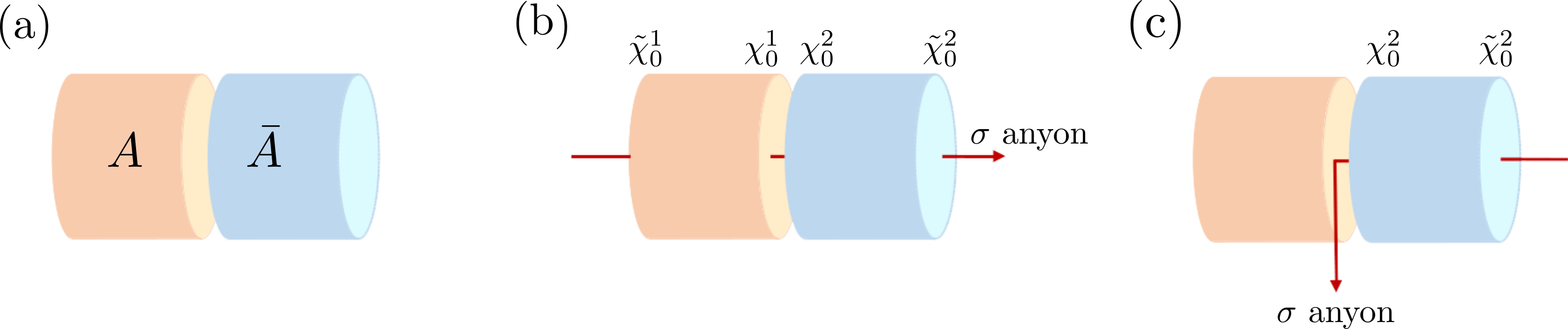
Figure 2: Flux insertion configurations considered in computation of the bipartite entanglement on the cylinder geometry. (a) No fluxes are inserted. All edge fermions obey NS boundary conditions. (b) A single $\pi$-flux, corresponding to the insertion of a $\sigma$ anyon flux, through the cylinder. All edge fermions obey R boundary conditions. (c) A single $\pi$-flux is inserted through the right half of the cylinder, but exits through the entanglement cut. The edge fermions on the left (right) cylinder obey NS (R) boundary conditions. In (b) and (c), the zero modes on the inner (outer) edge are $\chi_{0}^{1},\chi_{0}^{2}$ ($\bar{\chi}_{0}^{1},\bar{\chi}_{0}^{2}$).

We begin with a more detailed exposition of the cut-and-glue approach and explain the role of conformal boundary and vertex states, as well as how to construct them. For concreteness, we focus first the case of a chiral $p$-wave superconductor and then outline the simple extension of these methods to the case of a Chern insulator.

III.1.1 Bipartition and Ishibashi boundary states

The case of a bipartition was first considered in Ref. qi2012general , which we review here. Let us consider a chiral superconductor on an infinite spatial cylinder with an entanglement cut, partitioning the total system into two regions $A$ and $\bar{A}$ [Fig. 2(a)]. As described above, we physically cut the system along the entanglement cut, resulting in gapless edge modes on the boundaries of regions $A$ and $\bar{A}$, respectively. For the case of the chiral $p$-wave superconductor, they are described by chiral real (Majorana) fermion theories with opposite chiralities, denoted by $\gamma_{L}$ and $\gamma_{R}$. Their dynamics at low energies can be described by

$$H_{0} =\int_{0}^{2\pi}d\sigma\big{[}\gamma_{L}i\partial_{\sigma}\gamma_{L}+\gamma_{R}(-i\partial_{\sigma})\gamma^{\ }_{R}\big{]}.$$ (22)

Here, we take the circumference of the cylinder to be $L=2\pi$ for simplicity. The Majorana fermion fields obey either anti-periodic (Neveu-Schwarz, NS) or periodic (Ramond, R) boundary conditions. For later purposes, it is convenient to introduce

$$\psi^{1}(\sigma)\equiv\gamma^{\ }_{L}(\sigma),\quad\psi^{2}(\sigma)\equiv\gamma^{\ }_{R}(2\pi-\sigma).$$ (23)

The edge state Hamiltonian is then written as

$$H_{0} =\int_{0}^{2\pi}d\sigma\,\sum_{I=1,2}\psi^{I}i\partial_{\sigma}\psi^{I}.$$ (24)

The chiral Majorana fermion field $\psi(\sigma)$ can be Fourier expanded as

$$\psi(\sigma)=\sum_{s\in\mathbb{Z}+1/2}e^{-i\sigma s}\psi_{s}$$

$$\mbox{where}\quad\psi_{-s}=\psi_{s}^{\dagger},\quad\{\psi_{s},\psi_{s^{\prime}}\}=\delta_{s,-s^{\prime}}$$ (25)

in the NS sector. The vacuum of the NS sector is defined by

$$\psi_{s}|0\rangle=0\quad\mathrm{for}\quad s>0$$ (26)

We have a similar expansion for the R-sector with integer moding.

In order to “glue” the system back together, we introduce a tunneling term which gaps out the chiral edge degrees of freedom. Explicitly, we describe the gapped edge with the Hamiltonian $H_{0}+H_{int}$, where

$$H_{{\it int}} =im\int_{0}^{2\pi}d\sigma\,\gamma_{L}\gamma^{\ }_{R}=im\int_{0}^{2\pi}d\sigma\,\psi^{1}(\sigma)\psi^{2}(2\pi-\sigma).$$ (27)

As described above, we identify the entanglement between $A$ and $\overline{A}$ as arising purely from the entanglement between the chiral and anti-chiral Majorana fermions in this gapped state (i.e. the “left-right” entanglement das2015leftright ).

The gapped ground state is in fact related to a conformal boundary state, or more precisely, an Ishibashi state, $\ket{B}$, of the gapless theory described by $H_{0}$. For a general CFT, $\ket{B}$ is defined by the relation

$$\left[L_{n}-\bar{L}_{-n}\right]|B\rangle=0\quad(\forall n\in\mathbb{Z})$$ (28)

where $L_{n}$ ($\bar{L}_{n}$) is the Fourier component of the energy-momentum tensor $T(\sigma)$ ($\bar{T}(\bar{\sigma})$) of the edge theory. For the case of the free fermion theory, the Ishibashi state is defined by

$$\quad\left[\gamma^{\ }_{L}(\sigma)\mp i\gamma^{\ }_{R}(\sigma)\right]|B\rangle=0.$$ (29)

Or in terms of $\psi^{I}$,

$$[\psi^{1}(\sigma)\mp i\psi^{2}(2\pi-\sigma)]|B\rangle=0,$$ (30)

which is valid for the whole region $0\leq\sigma\leq 2\pi$ (this leads to $[\psi^{2}(\sigma)\pm i\psi^{1}(2\pi-\sigma)]|B\rangle=0$). Indeed we see that $\ket{B}$ is the ground state of $H$ in the limit $|m|\to\infty$. From the Ishibashi boundary state, we can approximate the ground state of the (2+1)d topological phase near the entanglement boundary for large but finite $m$ with the regularized state,

$$|G\rangle=\mathcal{N}e^{-\epsilon H_{0}}|B\rangle.$$ (31)

Here, the regulator $\epsilon$ is inversely proportional to the bulk energy gap. The reduced density matrix can then be constructed from $|G\rangle$ by tracing over $\bar{A}$, $\rho_{A}=\mathrm{Tr}_{\bar{A}}\,|G\rangle\langle G|.$ We emphasize that, while we took the non-interacting fermion theory as an example, essentially the same construction of the reduced density matrix using the Ishibashi boundary state can be done for a much broader class of theories.

The condition (30), $(\psi_{r}^{1}\mp i\psi_{-r}^{2})|B\rangle=0$, for the free fermion boundary state can explicitly be solved. For example, for the NS sector (the NS boundary condition), it is given in the form of a fermionic coherent state as:

$$|B\rangle=\exp\Big{(}i\sum_{r\geq 1/2}\psi_{-r}^{1}\psi_{-r}^{2}\Big{)}|0\rangle,$$ (32)

which has the form of Ishibashi state, as expected. Here $|0\rangle$ is the Fock vacuum defined by $\psi^{I}_{r}|0\rangle=0$ for $r>0$.

III.1.2 Multipartition and vertex states

The bipartite setup and the cut-and-glue method of the reduced density matrix presented above can be extended to a multipartition. In this section, we focus on a tripartition, but the following discussion can readily be extended to an $N$-partition ($N>3$). We first note that the configuration in Fig. 1(a) is topologically equivalent to the one obtained by first considering three cylinders, corresponding to the regions $A,B,C$, and then gluing these cylinders together [Fig. 3(a)]. As in the case of a bipartition, we cut open the system along the cut, resulting in an edge theory comprising three free Majorana fermions, as described by the Hamiltonian,

$$H_{0} =\int_{0}^{2\pi}d\sigma\sum_{I=1}^{3}\psi^{I}i\partial_{\sigma}\psi^{I}.$$ (33)

We again heal the cut by introducing tunneling terms of the form,

$$H_{{\it int}} =im\int_{0}^{\pi}d\sigma\sum_{I}\psi^{I+1}(\sigma)\psi^{I}(2\pi-\sigma),$$ (34)

such that the total Hamiltonian is $H_{0}+H_{{\it int}}$. (Here and henceforth, we use the convention $\psi^{4}\equiv\psi^{1}$). Analogously to the Ishibashi boundary state satisfying the condition (30), the ground state in the limit $|m|\to\infty$ is given by a conformal boundary state, $\ket{V}$, which satisfies

$$\big{[}\psi^{I+1}(\sigma)-i\psi^{I}(2\pi-\sigma)\big{]}|V\rangle=0,\quad 0\leq\sigma\leq\pi.$$ (35)

Solving the constraint, the state $|V\rangle$ is given in the form of a fermionic coherent state. These types of states, which we will refer to as vertex states, have been considered in the context of string field theory gross1987field ; gross1987operator ; gross1987operator2 ; leclair1989string where they describe the interaction among strings. As before, we regularize this state and consider $|G\rangle=\mathcal{N}e^{-\epsilon H_{0}}|V\rangle$, which provides an approximation to the ground state of $H$ for large but finite $|m|$. Once $|G\rangle$ is obtained, we can compute the reduced density matrices $\rho_{A\cup B},\rho_{B\cup C}$, and $\rho_{C\cup A}$ as well as the entanglement measures.

Although Eq. (35) uniquely defines the Majorana fermion vertex state, an equivalent and more general definition of vertex states, which also motivates the so-called Neumann coefficient approach to constructing them, proceeds as follows. In the interest of generality, we consider the most general case of an $N$-junction, such that $N$ edge theories meet at a single point. Hence, we start with $N$ copies of chiral CFTs (edge theories) defined on a spatial circle parameterized by $0\leq\sigma\leq 2\pi$. Their Hilbert spaces are denoted by $\mathcal{H}_{1,2,\ldots,N}$, respectively. Together with the (imaginary) time direction $\tau$, we have a cylindrical spacetime. As usual, we can map each theory to the conformal plane through the coordinate transformation $z=e^{\tau+i\sigma}$, such that the half of the cylinder $-\infty\leq\tau\leq 0$ is mapped to the unit disk, $|z|\leq 1$. We next consider conformal maps $\omega_{I}$ from the $I$-th unit disk to the complex plane $\mathbb{C}$ that are analytic inside the unit disk. In particular, they map each disk to a separate wedge of the complex plane $\mathbb{C}$, with the requirement that the edges of each wedge are flush with one another so that the desired boundary conditions are implemented. This sequence of maps for one disk is illustrated for the case $N=3$ in Fig. 3(b). We will elaborate more on this after we present the explicit form of the conformal maps momentarily. Then, we define a vertex state $|V\rangle\in\mathcal{H}_{1}\otimes\mathcal{H}_{2}\otimes\cdots\otimes\mathcal{H}_{N}$ by requiring it reproduce correlation functions on the complex plane as follows leclair1989string :

$$\langle V|\,\big{(}O_{\alpha}|0\rangle_{1}\otimes O_{\beta}|0\rangle_{2}\otimes\cdots\otimes O_{\gamma}|0\rangle_{N}\big{)}$$

$$=\big{\langle}\,\omega_{1}[O_{\alpha}]\,\omega_{2}[O_{\beta}]\,\cdots\,\omega_{N}[O_{\gamma}]\,\big{\rangle}_{\mathbb{C}}$$ (36)

where $|0\rangle_{I}$ is the vacuum in $\mathcal{H}_{I}$, $O_{\alpha,\beta,\cdots,\gamma}$ represents an arbitrary (primary) operator acting on $\mathcal{H}_{1,2,\cdots,N}$, $\omega_{I}[O]$ represents the transformation of a primary operator $O$ by $\omega_{I}$, $\omega_{I}[O(z)]=[\omega_{I}^{\prime}(z)]^{h}O(\omega_{I}(z))$, where $h$ is the conformal dimension of $O$. In order to fix the form of the conformal transformations $\omega_{I}$ which define the vertex state, we must impose additional constraints on $\ket{V}$. First, it is clear that, since the $N$ Hilbert space copies are equivalent, the vertex states must invariant under their cyclic permutation. That is to say, focusing on $N=3$,

$$\langle V_{123}|=\langle V_{231}|=\langle V_{312}|,$$ (37)

where the subscripts label the Hilbert space indices. Physically, this is just the statement that the trijunction is invariant under $120^{\circ}$ rotations. A second, less obvious requirement is given by, again focusing on $N=3$,

$$\langle V_{125}|\langle V_{5^{\dagger}34}|=\langle V_{235}|\langle V_{5^{\dagger}41}|,$$ (38)

The two sides of this expression correspond to gluing together two $N=3$ vertex states to obtain $N=4$ vertex states. This constraint expresses the fact that this $N=4$ vertex state must also be invariant under cyclic permutations of the Hilbert spaces (i.e. under $90^{\circ}$ rotations of the “tetrajunction”). Enforcing these constraints restricts the choice of conformal transformations $\omega_{I}$, which in turn define the vertex state $\ket{V}$. We next describe choices of the $\omega_{I}$ satisfying these constraints, which then lead to vertex states satisfying Eq. (35).

For $N=2$, we can choose the following conformal maps jevicki1988supersymmetry :

$$\omega_{I}(z)=\omega_{I,0}\frac{1+z}{1-z};\quad\omega_{I,0}=-ie^{i\pi I},\,I=1,2.$$ (39)

In this way, the first disk is mapped to the upper half plane and the second to the lower half plane. Note also that the infinite past $\tau=-\infty$ is mapped to $\pm i$, respectively. Here, we note that a quantum state at $\tau=0$ or $|z|=1$ can be obtained by a path integral from $\tau=-\infty$ or $|z|=0$ with possibly an insertion of an operator. By the conformal maps $\omega_{1,2}$, the $\tau=0$ slices of the disks are both mapped to the real axis. Hence, the field configurations for $\psi^{1}$ and $\psi^{2}$ are subject to the constraint in (30); we will show this more explicitly in the following subsection.

Likewise, for $N=3$, we can choose $\omega_{1,2,3}$ as

$$\omega_{I}(z)=\omega_{I,0}\left(\frac{1+z}{1-z}\right)^{\frac{2}{3}};\,\omega_{I,0}=e^{\frac{4\pi iI}{3}-i\pi},\,I=1,2,3.$$ (40)

Note that $\omega_{I}(2\pi-\sigma)=\omega_{I+1}(\sigma)$ for $0\leq\sigma\leq\pi$. These conformal maps bring three disks ($0\leq\sigma\leq 2\pi,\tau<0$) to the whole plane, such that each unit disk is mapped to a separate $120^{\circ}$ wedge of the conformal plane, as shown in Fig.  3(b) and Fig. 4(a). Here, the points at infinity are identified. We note that this construction is similar to, but slightly different from, the conformal maps used in open string field theory by Witten witten1986non ; the CFTs we consider obey (potentially twisted) periodic boundary conditions. Though this alternative definition of the vertex states seems obtuse at first glance, we will see in the following that it provides an elegant way of deriving the explicit form of said states.

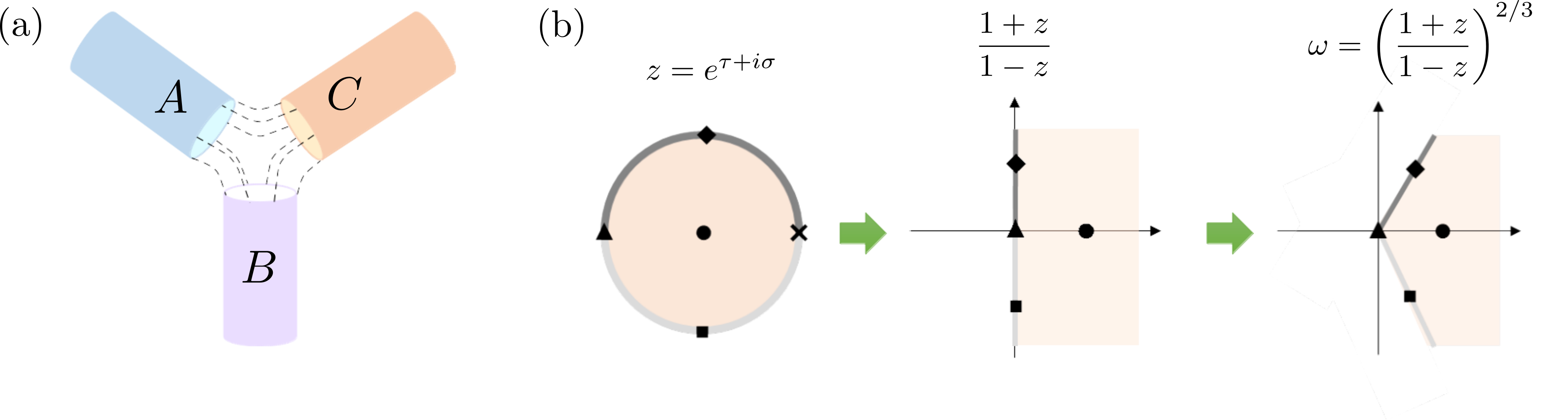
Figure 3: (a) Gluing three cylinders from edge theory point of view. (b) The conformal map used to define vertex states for tripartition. One disk ($0\leq\sigma\leq 2\pi,\tau<0$) is mapped to the one-third of the whole plane. The past infinity point $\tau=-\infty$, denoted by the black filled circle, is mapped to $\omega_{1,0}=e^{i\pi/3},\omega_{2,0}=e^{-i\pi/3},\omega_{3,0}=e^{-i\pi}$ for $I=1,2,3$ by Eq. (40).

III.1.3 The Neumann coefficient method

Let us now move on to the methods of constructing vertex states. On the one hand, the overlap condition (35) can be solved directly, and the vertex state can be constructed as a coherent state. We will discuss the direct construction in Appendix A and show the two methods give consistent results numerically.

On the other hand, the definition of vertex states (36) suggests the following strategy to construct vertex states, which we call the the Neumann coefficient method. For now, we focus on the NS sector for simplicity. We postulate the following Gaussian ansatz for $|V\rangle$:

$$|V\rangle=\exp\Big{(}\sum_{r,s\geq 1/2}\frac{1}{2}\psi_{-r}^{I}K_{rs}^{IJ}\psi_{-s}^{J}\Big{)}|0\rangle.$$ (41)

(Here and henceforth, we adopt the convention in which repeated flavor indices $I,J,\cdots$ are summed over implicitly, unless otherwise stated.) The coefficients $K_{rs}^{IJ}$ are chosen to reproduce the correlation function on the right-hand side of (36). Since $|V\rangle$ is Gaussian, it is sufficient to consider the two point functions of the fermion fields. We then consider, at $\tau=0$, the Neumann function

$$K^{IJ}(\sigma,\sigma^{\prime}) \equiv\langle\,\omega_{I}[\psi^{I}(\sigma)]\,\omega_{J}[\psi^{J}(\sigma^{\prime})]\,\rangle_{\mathbb{C}}$$

$$=\left(\frac{d\omega_{I}}{id\sigma}\right)^{1/2}\left(\frac{d\omega_{J}}{id\sigma^{\prime}}\right)^{1/2}\frac{1}{\omega_{I}-\omega_{J}}.$$ (42)

(Here, $I,J$ are not summed on the right hand side.) The Neumann coefficients $K_{rs}^{IJ}$ are related to the mode expansion of $K^{IJ}(\sigma,\sigma^{\prime})$ as

$$K^{IJ}(\sigma,\sigma^{\prime})=\sum_{r,s\geq 1/2}e^{ir\sigma}e^{is\sigma^{\prime}}K^{IJ}_{rs}+\delta_{IJ}\sum_{r\geq 1/2}e^{-ir(\sigma-\sigma^{\prime})}.$$ (43)

Note that there are two contributions to $K^{IJ}$: the regular piece that contains $K^{IJ}_{rs}$ and the singular piece $\delta_{IJ}\sum_{r\geq 1/2}e^{-ir(\sigma-\sigma^{\prime})}$. The presence of the singular piece is non-trivial, and needs to be verified case by case.

We now show the ansatz solution indeed satisfies the boundary condition (35). We first note that, with a proper choice of a branch in the conformal factor $(d\omega_{I}/id\sigma)^{1/2}$, the Neumann function satisfies

$$iK^{IJ}(2\pi-\sigma,\sigma^{\prime})=K^{I+1,J}(\sigma,\sigma^{\prime}),\quad 0\leq\sigma\leq\pi,$$ (44)

which reflects the cyclic constraint of Eq. (37). Using the mode expansion $\psi^{I}(\sigma)=\sum_{r}\psi_{r}^{I}e^{ir\sigma}$, $\psi^{I}(\sigma)|V\rangle$ can be expressed as

$$\psi^{I}(\sigma)|V\rangle$$ (45)

$$=\sum_{r\geq 1/2}\psi^{I}_{-r}e^{-ir\sigma}|V\rangle+\sum_{r,s\geq 1/2}e^{ir\sigma}K_{rs}^{IJ}\psi_{-s}^{J}|V\rangle$$

$$=\int\frac{d\sigma^{\prime}}{2\pi}K^{IJ}(\sigma,\sigma^{\prime})\psi_{\mathrm{cr.}}^{J}(\sigma^{\prime})|V\rangle,$$ (46)

where $\psi_{\mathrm{cr.}}^{I}(\sigma)=\sum_{r\geq 1/2}\psi^{I}_{-r}e^{-ir\sigma}$. Using the cyclic property of the Neumann function given in Eq. (44), we find,

$$\psi^{I}(2\pi-\sigma)|V\rangle =\int\frac{d\sigma^{\prime}}{2\pi}K^{IJ}(2\pi-\sigma,\sigma^{\prime})\psi_{\mathrm{cr.}}^{J}(\sigma^{\prime})|V\rangle$$

$$=(-i)\int\frac{d\sigma^{\prime}}{2\pi}K^{I+1,J}(\sigma,\sigma^{\prime})\psi_{\mathrm{cr.}}^{J}(\sigma^{\prime})|V\rangle$$

$$=-i\psi^{I+1}(\sigma)|V\rangle.$$ (47)

This completes the proof. Note that it was crucial to carefully take into account the singular part of the Neumann function. The proof presented here applies for the NS sector, and we leave the more complicated case of the R sector (Sec. IV.1.2) to Appendix B.1, B.2.

The direct and Neumann coefficient methods complement one other. When both methods can be applied, they give rise to the same (consistent) vertex states. We demonstrate the equivalence of these methods in the NS-NS-NS sector in Appendix A. In other sectors, because of the presence of zero modes, and because of the branch cuts, sometimes one method has an advantage over the other method. In general, vertex states obtained from these two methods are consistent, but may differ by an extra operator insertion at the junction imamura2006boundary ; imamura2008boundary .

III.1.4 Complex fermion

We close this subsection by commenting on the case of complex fermions, which parallels the treatment for real fermions. Indeed, the desired vertex state is obtained by combining two copies of real fermions. We consider complex fermion fields $f^{I}(\sigma),f^{I,{\dagger}}(\sigma)$. In the NS sector, they can be expanded as

$$f(\sigma)=\sum_{s\in\mathbb{Z}+1/2}e^{-i\sigma s}f_{s},\quad f^{\dagger}(\sigma)=\sum_{s\in\mathbb{Z}+1/2}e^{i\sigma s}f_{s}^{\dagger},$$

$$\qquad\mbox{with}\quad\{f^{\ }_{s},f_{s^{\prime}}^{\dagger}\}=\delta_{s,s^{\prime}}.$$ (48)

We have a similar mode expansion in the R-sector. We consider a vertex state obeying the overlap condition,

$$\big{[}f^{I+1}(\sigma)-if^{I}(2\pi-\sigma)\big{]}|V\rangle=0,$$

$$\big{[}f^{I+1,\dagger}(\sigma)-if^{I,\dagger}(2\pi-\sigma)\big{]}|V\rangle=0.$$ (49)

The complex fermion field $f,f^{\dagger}$ can be decomposed into two real fermion fields, $\psi$ and $\varphi$ as $f=(\psi-i\varphi)/\sqrt{2}$, $f^{\dagger}=(\psi+i\varphi)/\sqrt{2}$. Correspondingly, the Fourier modes of $f^{{\dagger}}$ and $f$, $f(\sigma)=\sum_{r}e^{ir\sigma}f_{r}$ ($\{f_{r}^{\dagger},f_{s}\}=\delta_{r,s}$), are related to the Fourier modes of $\psi$ and $\varphi$ as $f_{r}=(\psi_{r}-i\varphi_{r})/\sqrt{2},$, $f_{r}^{\dagger}=(\psi_{-r}+i\varphi_{-r})/\sqrt{2}.$ The ansatz solution is then

$$|V\rangle =\exp{\Big{(}\frac{1}{2}\sum_{r,s\geq 1/2}\psi_{-r}^{I}K_{rs}^{IJ}\psi_{-s}^{J}+\varphi_{-r}^{I}K_{rs}^{IJ}\varphi_{-s}^{J}\Big{)}}|0\rangle$$ (50)

$$=\exp{\Big{(}\sum_{r,s\geq 1/2}f_{r}^{I\dagger}K_{rs}^{IJ}f_{-s}^{J}\Big{)}}|0\rangle.$$

The treatment of the R sector follows similarly, although we need to take into account the presence of zero modes properly, as we shall see in the following subsections.

III.2 Bipartition

In this subsection, we consider the bipartitions of a chiral $p$-wave superconductor and a Chern insulator, using the Neumann coefficient method described above. As mentioned at the beginning of this section, we investigate the effect of inserting non-trivial $\pi$-fluxes through the cylinder on the entanglement. As shown in Fig. 2, we consider the insertion of (a) no flux (b) $\pi$-flux through the cylinder, and (c) a $\pi$-flux through one end of the cylinder, which exits through the entanglement cut. For the chiral superconductor, a $\pi$-flux is an extrinsic defect which traps a Majorana zero-mode, forming an Ising anyon. Thus, (b) can be viewed as creating a pair of Ising anyons in the bulk and dragging them to opposite ends of the cylinder, while (c) results from dragging only one Ising anyon to an edge and leaving the other in the bulk. In the bulk language, the creation and manipulation of the Ising anyons leaves behind a Wilson line on the cylinder or, equivalently, an anyon flux through the cylinder. At the level of the edge theories, the braiding of the Majorana fermions around the Ising anyon flux results in a phase of $-1$. Hence, the three configurations in Fig. 2 are described by the boundary condition sectors of the edge theories: (a) NS-NS, in which all fermions obey anti-periodic boundary conditions (b) R-R, in which all fermions obey periodic boundary conditions, and (c) NS-R, in which the fermions on the left (right) cylinder obey anti-periodic (periodic) boundary conditions. We compute the entanglement in each sector in turn. As is well-established, we obtain an area law for case (a) and an area law term plus a subleading $\ln\sqrt{2}$ correction from the Ising anyons for case (b), which requires a careful treatment of the zero modes yao2010entanglement ; sohal2020nonabelian ; lim2021disentangling . The case (c) has not been considered before and we find a novel subleading correction to the entanglement.

III.2.1 The NS-NS sector

The setup of the calculation for the NS-NS sector is already outlined above; all that remains is to explicitly evaluate the Neumann functions. Noting $\frac{d\omega_{I}}{id\sigma}=\frac{2z\omega_{I,0}}{(1-z)^{2}}$ and choosing the branch cuts carefully ($\sqrt{\omega_{1,0}}=\sqrt{i},\sqrt{\omega_{2,0}}=i\sqrt{i}$, which leads to $\sqrt{\omega_{1,0}\omega_{2,0}}=-1$), we obtain:

$$K^{11} =K^{22}=\frac{\sqrt{zz^{\prime}}}{z-z^{\prime}}=\sum_{r\geq 1/2}e^{-ir(\sigma-\sigma^{\prime})},$$ (51)

$$K^{12} =-K^{21}=\frac{i\sqrt{zz^{\prime}}}{1-zz^{\prime}}=i\sum_{r\geq 1/2}e^{ir(\sigma+\sigma^{\prime})}.$$

Note that $K^{11}=K^{22}$ yields the expected singularity. We also note that under $\sigma\rightarrow 2\pi-\sigma$ ($z\rightarrow 1/z$, $\sqrt{z}\rightarrow-1/\sqrt{z}$), the Neumann function satisfies $K^{1J}(2\pi-\sigma,\sigma^{\prime})+iK^{2J}(\sigma,\sigma^{\prime})=0$ and $K^{2J}(2\pi-\sigma,\sigma^{\prime})-iK^{1J}(\sigma,\sigma^{\prime})=0$ for $0\leq\sigma\leq 2\pi$. From the expansion of $K^{12}$, we conclude $K^{12}_{rs}=-K^{21}_{rs}=\delta_{rs}$. Plugging this into Eq. (41), we obtain the Ishibashi state (32) as expected.

III.2.2 The R-R sector

Let us now consider the vertex state in the R-R sector. We denote the fermion fields with the R boundary condition as $\chi^{I}(\sigma)$. As before, the vertex state satisfies

$$[\chi^{1}(\sigma)+i\chi^{2}(2\pi-\sigma)]|V\rangle$$

$$=[\chi^{2}(\sigma)-i\chi^{1}(2\pi-\sigma)]|V\rangle=0$$ (52)

for $0\leq\sigma\leq 2\pi$. In the bulk, this situation corresponds to a flux or, Ising anyon Wilson line, threading the hole of the cylinder [Fig. 2 (b)]. From the edge theory point of view, we need to include suitable twist operators to introduce branch cuts, which enforce periodic boundary conditions for the fermions. This will modify the Neumann function, which we now denote as $R^{IJ}$. It is related to the Neumann function in the NS sector via:

$$R^{IJ}(\sigma,\sigma^{\prime})=K^{IJ}(\sigma,\sigma^{\prime})g^{IJ}(\sigma,\sigma^{\prime}),$$ (53)

where $g^{IJ}$ is the new factor arising from the branch cuts. (Here, the summation convention does not apply in the right hand side.) We work with the following choice of the branch cuts,

$$g^{IJ}=\frac{1}{2}\left[\sqrt{\frac{(\omega_{I}-\omega_{1,0})(\omega^{\prime}_{J}-\omega_{2,0})}{(\omega^{\prime}_{J}-\omega_{1,0})(\omega_{I}-\omega_{2,0})}}+(\omega_{I}\leftrightarrow\omega^{\prime}_{J})\right],$$ (54)

where we recall $\omega_{1,0}=i,\omega_{2,0}=-i$. Other choices are also possible and give an identical vertex state, as we demonstrate in Appendix B.1. Using the conformal map in Eq. (39), the explicit form of $g^{IJ}$ is

$$g^{11} =g^{22}=\frac{1}{2}\left(\sqrt{\frac{z}{z^{\prime}}}+\sqrt{\frac{z^{\prime}}{z}}\right),$$ (55)

$$g^{12} =g^{21}=\frac{1}{2}\left(\sqrt{zz^{\prime}}+\frac{1}{\sqrt{zz^{\prime}}}\right).$$

These functions satisfy $g^{1J}(\sigma,\sigma^{\prime})=-g^{2J}(2\pi-\sigma,\sigma^{\prime})$ (using $z\rightarrow 1/z,\sqrt{z}\rightarrow-1/\sqrt{z}$). The Neumann function is:

$$R^{11} =R^{22}=\frac{1}{2}\frac{z+z^{\prime}}{z-z^{\prime}}=\frac{1}{2}+\sum_{n\geq 1}e^{-in(\sigma-\sigma^{\prime})},$$ (56)

$$R^{12} =-R^{21}=\frac{i}{2}\frac{1+zz^{\prime}}{1-zz^{\prime}}=\frac{i}{2}+i\sum_{n\geq 1}e^{in(\sigma+\sigma^{\prime})}.$$

They satisfy $R^{1J}(2\pi-\sigma,\sigma^{\prime})-iR^{2J}(\sigma,\sigma^{\prime})=R^{2J}(2\pi-\sigma,\sigma^{\prime})+iR^{1J}(\sigma,\sigma^{\prime})=0$. Again, the correct singular terms show up in $R^{11}$ and $R^{22}$. The solution for $|V\rangle$ for real fermions in the R-R sector is then

$$|V\rangle=\exp\Big{(}-i\sum_{n\geq 1}\chi_{-n}^{1}\chi_{-n}^{2}\Big{)}|\Omega\rangle,$$ (57)

with an additional requirement $[\chi_{0}^{1}+i\chi_{0}^{2}]|\Omega\rangle=0$. One can verify that they satisfy the boundary condition (III.2.2). The requirement that $|V\rangle$ has definite parity for the zero mode can also be understood from the $i/2$ term in $R^{12}$.

The zero modes $\chi_{0}^{1},\chi_{0}^{2}$ of the real fermion need to be handled with extra care. $\chi_{0}^{1},\chi_{0}^{2}$ live on the inner edges of the cylinders. To have a well-defined Hilbert space, we also need to include the zero modes on the outer edges of the cylinders, which we denote as $\bar{\chi}_{0}^{1},\bar{\chi}_{0}^{2}$, as shown in Fig. 2(b). Indeed, we recall that before making a physical cut along the entanglement cut, the cylinder with an Ising anyon flux passing through it is topologically equivalent to a sphere with a pair of Ising anyon defects. The anyons yield a double degeneracy, as each has quantum dimension $\sqrt{2}$. This corresponds to choosing whether the complex fermion formed from the corresponding zero modes, $\bar{\chi}_{0}^{1}+i\bar{\chi}_{0}^{2}$, is occupied or unoccupied. We must make a choice of which state in this degenerate subspace we wish to compute the entanglement for. For concreteness, we choose the state in which this fermion is unoccupied, which amounts to imposing the boundary condition $[\bar{\chi}_{0}^{1}+i\bar{\chi}_{0}^{2}]|\Omega\rangle=0$ for the outer edge zero modes. If we define the complex fermion

$$g_{i}=\frac{1}{\sqrt{2}}(\chi_{0}^{1}+i\chi_{0}^{2}),\quad g_{o}=\frac{1}{\sqrt{2}}(\bar{\chi}_{0}^{1}+i\bar{\chi}_{0}^{2}),$$ (58)

the zero-mode vacuum state is $|\Omega\rangle=|0_{i},0_{o}\rangle$. This completes the construction of the boundary state.

Note that $g_{i}$ and $g_{o}$ mix the Hilbert spaces of the left and right cylinders. When we compute the entanglement we must trace out one of these cylinders, and so it is necessary to perform a change of basis to complex fermion modes localized on either the left or right cylinder: $g_{A}=(\chi_{0}^{1}+i\bar{\chi}_{0}^{1})/\sqrt{2},\$ $g_{B}=(\chi_{0}^{2}+i\bar{\chi}_{0}^{2})/\sqrt{2}.$ In this basis, the vacuum is a maximally entangled state:

$$|\Omega\rangle=|0_{i},0_{o}\rangle=(|0_{A}0_{B}\rangle-i|1_{A}1_{B}\rangle)/\sqrt{2}.$$ (59)

Below, we will see this gives a contribution of $\ln{2}$ to the entanglement entropy.

III.2.3 The NS-R sector

Finally, we consider the NS-R sector which, as described above, describes a novel configuration in which we insert an anyon flux through one end of the cylinder which then exits through the entanglement cut. From Fig. 2(c), we see that the fermions on the right cylinder braid around the anyon flux and so obey R boundary conditions, whereas the fermions on the left cylinder do not and hence are in the NS sector. In order to describe the gapped edge state at the entanglement cut, we must impose a modified boundary condition:

$$[\psi(\sigma)+i\mathrm{sgn}(\pi-\sigma)\chi(2\pi-\sigma)]\ket{V}=0,$$ (60)

for $0\leq\sigma<2\pi$. Here, $\psi$ ($\chi$) obeys NS (R) boundary conditions. Formally, the sign function is needed to ensure the above expression is well-defined under shifts of $\sigma\to\sigma+2\pi$. Physically, it represents the fact that an anyon flux is piercing the entanglement cut. Indeed, the Ising twist field is precisely the operator at the level of the edge CFT which introduces such a “kink” for the Majorana fields.

To the best of our knowledge, the vertex state in this case was first constructed in jevicki1988supersymmetry . In the NS-R sector, we only need to introduce the branch cut for the second string. The branch cut factor $g^{IJ}$ is chosen as jevicki1988supersymmetry :

$$g^{IJ}(\sigma,\sigma^{\prime})=\frac{1}{2}\left[\sqrt{\frac{\omega_{I}-\omega_{2,0}}{\omega^{\prime}_{J}-\omega_{2,0}}}+\sqrt{\frac{\omega^{\prime}_{J}-\omega_{2,0}}{\omega_{I}-\omega_{2,0}}}\right].$$ (61)

Explicitly,

$$g^{11} =\frac{1}{2}\left(\sqrt{\frac{1-z^{\prime}}{1-z}}+\sqrt{\frac{1-z}{1-z^{\prime}}}\right),$$ (62)

$$g^{12} =\frac{i}{2}\left(\sqrt{\frac{1-z^{\prime}}{1-z}}\frac{1}{\sqrt{z^{\prime}}}-\sqrt{z^{\prime}}\sqrt{\frac{1-z}{1-z^{\prime}}}\right),$$

$$g^{22} =\frac{1}{2}\left(\sqrt{\frac{1-z^{\prime}}{1-z}}\sqrt{\frac{z}{z^{\prime}}}+\sqrt{\frac{1-z}{1-z^{\prime}}}\sqrt{\frac{z^{\prime}}{z}}\right).$$

$R^{IJ}$ satisfies $R^{IJ}(\sigma,\sigma^{\prime})=-iR^{I+1,J}(2\pi-\sigma,\sigma^{\prime})$ for $0\leq\sigma\leq\pi$. The mode expansion of $R^{IJ}$ needed to extract the $R^{IJ}_{rs}$ in the definition of the vertex state, takes a more complicated form than that of the preceding two cases:

$$R_{rs}^{11} =\frac{r-s}{2(r+s)}u_{2r-1}u_{2s-1},$$ (63)

$$R_{rn}^{12} =-R^{21}_{nr}=\frac{n+r}{2(n-r)}u_{2r-1}u_{2n},$$

$$R_{nm}^{22} =\frac{n-m}{2(n+m)}u_{2n}u_{2m},$$

where $u_{n}$ is the expansion coefficients of $u(x)$:

$$u(x)=\sqrt{\frac{1+x}{1-x}}=\sum_{n=0}^{\infty}u_{n}x^{n}.$$ (64)

Making use of this mode expansion and separating the oscillator and zero-mode contributions, we can write out the vertex state of Eq. (41) as

$$|V\rangle =\exp\Big{(}\sum_{r,s\geq 1/2}\frac{1}{2}\psi_{-r}R^{11}_{rs}\psi_{-s}+\sum_{m,n\geq 1}\frac{1}{2}\chi_{-n}R^{22}_{nm}\chi_{-m}$$ (65)

$$\qquad+\sum_{r\geq 1/2,n\geq 1}\psi_{-r}R^{12}_{rn}\chi_{-n}+\sum_{r\geq 1/2}2\psi_{-r}R^{12}_{r0}\chi_{0}+\sum_{n\geq 1}2\chi_{-n}R^{22}_{n0}\chi_{0}\Big{)}|\Omega\rangle.$$

Now, as in the R-R sector, to fix the form of the vacuum $\ket{\Omega}$, we must treat the zero-mode sector carefully. Indeed, due to the $\pi$ flux through one half of the cylinder, we have another zero mode, $\bar{\chi}_{0}$, on the outer edge of the left cylinder [Fig. 2(c)]. We can combine them to define the complex fermion operator $g_{0}$:

$$g_{0}=\frac{1}{\sqrt{2}}(\chi_{0}-i\bar{\chi}_{0}),\quad g_{0}^{\dagger}=\frac{1}{\sqrt{2}}(\chi_{0}+i\bar{\chi}_{0}).$$ (66)

Now, prior to making the entanglement cut, this flux configuration is again topologically equivalent to a sphere supporting a pair of Ising anyons, corresponding to the $\chi_{0}$ and $\bar{\chi}_{0}$ zero modes, yielding a double degeneracy associated with the occupation of $g_{0}$. (Note that, in contrast to the R-R case, cutting the system along the entanglement cut does not introduce additional zero modes). We must again make a choice of which state in which to compute the entanglement. We can fix the state by choosing a value for the occupation number of $g_{0}$ of the reference state $\ket{\Omega}$; for simplicity, we take $g_{0}$ to be unoccupied, so that $\ket{\Omega}=\ket{0}$. Finally, to simplify the expression for the vertex state, we observe that $X\equiv\sqrt{2}(\sum_{r\geq 1/2}\psi_{-r}R_{r0}^{12}+\sum_{n\geq 1}\chi_{-n}R^{22}_{n0})g_{0}^{\dagger}$ and $Y\equiv\sqrt{2}(\sum_{r\geq 1/2}\psi_{-r}R_{r0}^{12}+\sum_{n\geq 1}\chi_{-n}R^{22}_{n0})g_{0}$, commute, $[X,Y]=0$, and hence $e^{X+Y}=e^{X}e^{Y}$. The vertex state thus takes the form

$$|V\rangle= \exp\Big{(}\sum_{r,s\geq 1/2}\frac{1}{2}\psi_{-r}R_{rs}^{11}\psi_{-s}+\sum_{m,n\geq 1}\frac{1}{2}\chi_{-n}R^{22}_{nm}\chi_{-m}$$ (67)

$$\qquad+\sum_{r\geq 1/2,n\geq 1}\psi_{-r}R^{12}_{rn}\chi_{-n}+\sqrt{2}(\sum_{r\geq 1/2}\psi_{-r}R_{r0}^{12}+\sum_{n\geq 1}\chi_{-n}R^{22}_{n0})g_{0}^{\dagger}\Big{)}|0\rangle.$$

III.2.4 Entanglement entropy

Having constructed the relevant boundary states for the NS-NS, R-R, NS-R sectors, we now proceed to compute the entanglement entropy $S_{A}$ after tracing out one half of the cylinder. Let us start with the NS-NS sector. We recall that the ground state of the entanglement interface is given by a regularized version of the boundary state, as stated in Eq. (31); this amounts to replacing $\psi_{-r}^{I}\rightarrow\psi_{-r}^{I}e^{-\epsilon r}$ in Eq. (32). The entanglement entropy can directly be evaluated as

$$S =\left(1-\epsilon\frac{d}{d\epsilon}\right)\ln{[\prod_{r\geq 1/2}(1+q^{r})]}$$ (68)

where $q=e^{2\pi i\tau}=e^{-4\epsilon}$ and $\tau=\frac{2i\epsilon}{\pi}$. We can write the argument of the logarithm in terms of the Dedekind $\eta$ function and a Jacobi $\theta$ function:

$$\prod_{r\geq 1/2}(1+q^{r})=q^{1/48}\sqrt{\frac{\theta_{3}(\tau)}{\eta(\tau)}}.$$ (69)

Under the modular $\mathcal{S}$ transformation and taking the limit $\epsilon\rightarrow 0$ limit (which corresponds to taking the bulk gap to be very large), we have:

$$\frac{\theta_{3}(\tau)}{\eta(\tau)}=\frac{\theta_{3}(-\frac{1}{\tau})}{\eta(-\frac{1}{\tau})}\rightarrow\frac{1}{(e^{-\frac{2\pi i}{\tau}})^{1/24}}=e^{\frac{\pi^{2}}{24\epsilon}}.$$ (70)

We thus find,

$$S_{NS-NS}^{\mathrm{Real.}}\rightarrow\frac{\pi(1/2)}{24}\frac{L}{\epsilon}\quad\mbox{as}\quad\frac{L}{\epsilon}\rightarrow\infty,$$ (71)

as expected. Here, we reinstated the IR length scale $L$ (which has been set to $2\pi$ for simplicity) to make the area law form of the entropy more explicit and so that the dimensions are correct. We also make the chiral central charge $c=1/2$ dependence explicit.

The entanglement entropy in the R-R sector can be computed similarly. However, the presence of the zero modes make the calculations slightly more subtle. Let us first compute the contribution from the oscillator modes $n\geq 1$. With the regulator $\epsilon$, it can be computed as

$$S_{\mathrm{oscil.}}=\left(1-\epsilon\frac{d}{d\epsilon}\right)\ln{[\prod_{n\geq 1}(1+q^{n})]}.$$ (72)

The product can be identified with $\theta_{2}$ function:

$$\prod_{n\geq 1}(1+q^{n})=\frac{1}{\sqrt{2}}\sqrt{\frac{\theta_{2}(\tau)}{\eta(\tau)}}q^{-1/24}.$$ (73)

Under the modular $\mathcal{S}$ transformation and again taking the limit $\epsilon\rightarrow 0$, we have:

$$\frac{\theta_{2}(\tau)}{\eta(\tau)}=\frac{\theta_{4}(-\frac{1}{\tau})}{\eta(-\frac{1}{\tau})}\rightarrow\frac{1}{(e^{-\frac{2\pi i}{\tau}})^{1/24}}=e^{\frac{\pi^{2}}{24\epsilon}}.$$ (74)

This gives

$$S_{\mathrm{oscil.}}=\frac{\pi(1/2)}{24}\frac{L}{\epsilon}-\frac{1}{2}\ln{2}.$$ (75)

For the zero mode part, after the basis transformation, the vacuum takes the form of a maximally entangled state, $|\Omega\rangle=|0_{i},0_{o}\rangle=(|0_{A}0_{B}\rangle-i|1_{A}1_{B}\rangle)/\sqrt{2},$ which gives a contribution of $\ln{2}$. Summing up these two terms, the total entanglement entropy is:

$$S_{R-R}^{\mathrm{Real.}}=\frac{\pi(1/2)}{24}\frac{L}{\epsilon}+\ln{\sqrt{2}}.$$ (76)

Compared with $S_{NS-NS}^{\mathrm{Real.}}$, the extra contribution $\ln{\sqrt{2}}$ is exactly the topological entanglement entropy from the $\sigma$ anyon, as expected yao2010entanglement .

$\epsilon$	0.005	0.008	0.01	0.02
$S^{\mathrm{Real.}}_{R-R}$	82.5933	51.7508	41.4699	20.9082
$S^{\mathrm{Real.}}_{R-NS}$	82.3433	51.5008	41.2199	20.6582
$\Delta S$	0.2500	0.2500	0.2500	0.2500

Table 1: $S^{\mathrm{Real.}}_{R-R}$ and $S^{\mathrm{Real.}}_{R-NS}$ for various choices of $\epsilon$. For each fixed $\epsilon$, we increase cutoff $N$ until $S$ saturates. We observe that the difference $\Delta S=S^{\mathrm{Real.}}_{R-R}-S^{\mathrm{Real.}}_{R-NS}$ is a constant.

We now proceed to the NS-R case. Since the entanglement entropy in this case is not amenable to analytical calculations, we will perform a numerical computation using the correlation matrix method introduced in Section II.1 with a cutoff of mode $N_{c}$. For a given value of $\epsilon$, we take $N_{c}$ to be sufficiently large such that $S_{A}$ does not appreciably change with further increases in $N_{c}$. We collect the results in Table 1. We observe that the area law contributions ($O(L/\epsilon)$) to $S^{\mathrm{Real.}}_{R-R}$ and $S^{\mathrm{Real.}}_{NS-R}$ cancel out exactly, and the difference

$$\Delta S=S^{\mathrm{Real.}}_{R-R}-S^{\mathrm{Real.}}_{R-NS}=0.2500$$ (77)

appears to be remarkably well quantized. Now, we recall that, in the R-R sector, the presence of the anyon flux passing through the cylinder (i.e. the presence of Ising anyons on the ends of the cylinder) led to a contribution of $\Delta S_{0}=S^{\mathrm{Real.}}_{R-R}-S^{\mathrm{Real.}}_{NS-NS}=\ln{\sqrt{2}}=0.3466$ to the entanglement entropy over the NS-NS case, in which there was no flux. We see that $0<\Delta S<\Delta S_{0}$. This seems reasonable, as one expects the two halves of the cylinder in the present NS-R case where one Ising anyon straddles entanglement cut to somehow be less entangled than the R-R case, where the Ising anyons are located deep in the bulks of the two subregions. Evidently, $\Delta S_{0}-\Delta S=0.0966$ corresponds to a contribution to the entanglement from the anyon flux which pierces the entanglement cut. We should, however, perhaps be careful in identifying this as a universal contribution, as this cut-and-glue approach likely corresponds to a particular choice of regularization of how the anyon flux pierces the cut. The value of this new topological contribution may depend on this regularization. Additionally, we note that the examination of the entanglement spectrum in the NS-R sector shows that levels are all equally spaced with no degeneracy. The equal spacing structure encodes the CFT signature.

Finally, we consider the entanglement entropy for the case of complex fermion, i.e., the edge theory of a Chern insulator with unit Hall conductivity, and make a comparison with the above results. In the NS-NS sector, the entanglement entropy for the complex fermion is simply twice as large as the real fermion case,

$$S_{NS-NS}^{\mathrm{Cplx.}}=2S_{NS-NS}^{\mathrm{Real.}}=\frac{\pi}{24}\cdot\frac{L}{\epsilon}.$$ (78)

In the R-R sector, we need to include the effect of the fermion zero modes properly, while the treatment for the oscillator part is essentially the same. For the zero mode part, since $\chi_{0}$ is already a well-defined degree of freedom, paired with $\chi_{0}^{\dagger}$, we can only consider the inner edges. The vacuum $|\Omega\rangle$ needs to satisfy $(\chi_{0}^{1}-i\chi_{0}^{2})|\Omega\rangle=0,(\chi_{0}^{1,\dagger}-i\chi_{0}^{2,\dagger})|\Omega\rangle=0$, which can be chosen as $|\Omega\rangle=(\chi_{0}^{2,\dagger}+i\chi_{0}^{1,\dagger})|0\rangle.$ This is a maximally-entangled pair state and gives $S_{0}=\ln{2}$ contribution to $S$. To sum up,

$$S_{R-R}^{\mathrm{Cplx.}}=2S_{\mathrm{oscil.}}+S_{0}=\frac{\pi}{24}\cdot\frac{L}{\epsilon}.$$ (79)

There is no topological contribution for the complex fermion. Furthermore, the numerical calculation of the NS-R case shows $S_{NS-NS}^{\mathrm{Cplx.}}=S_{NS-R}^{\mathrm{Cplx.}}=S_{R-R}^{\mathrm{Cplx.}}.$ This is desired since we expect $S_{NS-R}^{\mathrm{Cplx.}}$ to lie between $S_{NS-NS}^{\mathrm{Cplx.}}$ and $S_{R-R}^{\mathrm{Cplx.}}$. Once again, the NS-R entanglement spectrum shows equal spacing behavior with no degeneracy.

IV Tripartite vertex states and entanglement

Having illustrated how the Neumann coefficient method reproduces the expected boundary states and entanglement entropy for a bipartition on the cylinder with and without flux threading it, as well as having derived a new result for the entanglement in the case where a flux pierces the cut, we turn to the main focus of this work, namely the entanglement for a tripartition [Fig. 1(b)]. We will again focus primarily on the case of a chiral $p$-wave superconductor and consider the effect of inserting $\pi$-fluxes through the cylinders. In particular, we investigate the entanglement when no fluxes are inserted and when two fluxes are inserted through two cylinders such that one flux exits through the remaining cylinder and the other flux through the entanglement cut [Fig. 4(a)]. At the level of the edge theories, these correspond to the NS-NS-NS and R-R-R sectors, respectively. We construct the vertex states for each case next before discussing the tripartite entanglement measures introduced in Sec. II.

As a complement to the Neumann coefficient approach, we also introduce a direct calculation method for computing the vertex state in Sec. A. We show these two methods give identical results for the vertex state solution numerically.

IV.1 Vertex states

IV.1.1 The NS-NS-NS sector

We first consider the simplest case in which no fluxes are inserted through the cylinders. The required vertex state $\ket{V}$ is given by the Gaussian ansatz of Eq. (41), the construction of which is outlined in Sec. III.1.3. All that remains is to determine the explicit form of the Neumann coefficients from the correlation function, Eq. (III.1.3). The conformal factor in Eq. (III.1.3) is given explicitly as $(\frac{d\omega_{I}}{id\sigma})^{1/2}=\frac{1}{\omega_{I}^{1/4}}(\frac{(\omega_{I}^{3}+1)}{3})^{1/2}$. We choose the branch such that $\omega_{I}^{1/4}(2\pi-\sigma)=i\omega_{I+1}^{1/4}(\sigma)$. This can be achieved by the following choice:

$$\omega_{I}^{1/4}(\sigma)=\tilde{\omega}_{I}\left(\frac{1+e^{i\sigma}}{1-e^{i\sigma}}\right)^{1/6}$$

$$\mbox{with}\quad\tilde{\omega}_{1}=e^{i\pi/12},\quad\tilde{\omega}_{2}=e^{-i7\pi/12},\quad\tilde{\omega}_{3}=e^{i3\pi/4}.$$ (80)

The explicit form of the Neumann coefficients $K^{IJ}_{rs}$ is technically involved and not particularly physically illuminating, and so we relegate it to Appendix B.3.

IV.1.2 The R-R-R sector

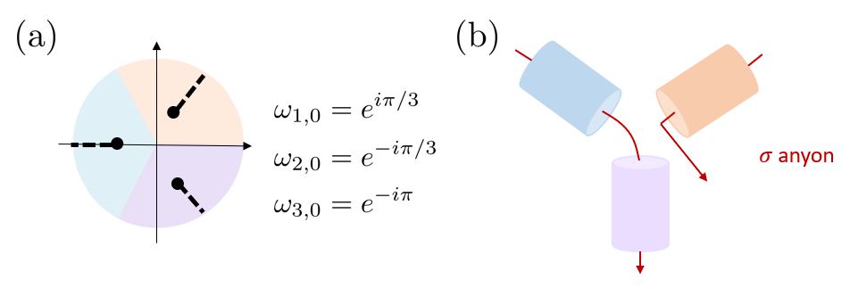
Figure 4: (a) The $\sigma$ anyon flux insertion in the R-R-R sector. One $\sigma$-anyon is forced to be exited at the junction. (b) The choice of the branch cuts for the R-R-R sector tripartition vertex state. The branch cuts connect $\omega_{I,0}$ to $\infty$.

Next we consider the case in which all fermions are in the R sector. Similar to the NS-R sector discussed for the case of a bipartition, in the R-R-R sector, the conservation of topological charge enforces the presence of an Ising anyon at the junction where all three entanglement boundaries meet. From the edge theory point of view, we must again compute the Neumann functions for periodic fermions, which takes the form in Eq. (53) with the factor $g^{IJ}$ accounting for the branch cuts. We choose to work with the branch cut configuration in Fig. 4(b).

To determine the branch cut factor $g^{IJ}(\sigma,\sigma^{\prime})$, the following general properties should be satisfied ginsparg1988applied : (i) $\omega$ and $\omega^{\prime}$ are symmetric in $g^{IJ}$ (thus anti-symmetric in $R^{IJ}$); (ii) The branch points include $\omega_{1,0}$, $\omega_{2,0}$, and $\omega_{3,0}$; (iii) $g$ reduces to 1 when $\omega^{\prime}\rightarrow\omega$, so $R^{IJ}$ reduces to $K^{IJ}$ in this limit. Furthermore, for our specific problem, $R^{IJ}$ should also satisfy: (iv) The singular term in $R^{IJ}$ must be $\delta^{IJ}\sum_{n\geq 1}e^{-in(\sigma-\sigma^{\prime})}$ to ensure the boundary condition is properly satisfied, as we show in Appendix B.2. This extra requirement is non-trivial, and may rule out some of the candidates that satisfy (i-iii).

We propose to use the following branch cut factor:

$$g^{IJ}(\sigma,\sigma^{\prime})=\frac{1}{2} \left[\left(\frac{(\omega_{I}-\omega_{1,0})(\omega_{I}-\omega_{2,0})(\omega_{I}-\omega_{3,0})}{(\omega_{J}^{\prime}-\omega_{1,0})(\omega_{J}^{\prime}-\omega_{2,0})(\omega_{J}^{\prime}-\omega_{3,0})}\right)^{1/2}\right.$$ (81)

$$+ \left.\left(\frac{(\omega_{J}^{\prime}-\omega_{1,0})(\omega_{J}^{\prime}-\omega_{2,0})(\omega_{J}^{\prime}-\omega_{3,0})}{(\omega_{I}-\omega_{1,0})(\omega_{I}-\omega_{2,0})(\omega_{I}-\omega_{3,0})}\right)^{1/2}\right],$$

where $\omega_{1,0}=e^{i\pi/3},\omega_{2,0}=e^{-i\pi/3},\omega_{3,0}=e^{-i\pi}$, and $\omega_{I}(\sigma),\omega_{J}^{\prime}(\sigma^{\prime})$ are defined in Eq. (40). It is easy to check that this candidate fulfills the requirements (i-iii). The branch points also include $\infty$. The branch cuts can be chosen from $\omega_{1,0}$ to $\infty$, $\omega_{2,0}$ to $\infty$, and $\omega_{3,0}$ to $\infty$, as shown in Fig. 4(b). We will compute the singular terms explicitly later, which verifies requirement (iv). It turns out that $g^{IJ}$ is the same for any $I,J$, and the mode expansion of $g^{IJ}$ in powers of $z=e^{i\sigma}$ is given by

$$g^{IJ} =\frac{1}{2}\left[\big{(}\frac{1}{\sqrt{z^{\prime}}}-\sqrt{z^{\prime}}\big{)}\sum_{r\geq 1/2}z^{r}+\big{(}\frac{1}{\sqrt{z}}-\sqrt{z}\big{)}\sum_{r\geq 1/2}z^{\prime r}\right]$$

$$=\frac{1}{2}\sum_{m=0}^{\infty}\left[e^{i\sigma(\frac{1}{2}+m)-i\frac{\sigma^{\prime}}{2}}-e^{i\sigma(\frac{1}{2}+m)+i\frac{\sigma^{\prime}}{2}}\right.$$

$$\qquad\qquad+\left.e^{i\sigma^{\prime}(\frac{1}{2}+m)-i\frac{\sigma}{2}}-e^{i\sigma^{\prime}(\frac{1}{2}+m)+i\frac{\sigma}{2}}\right].$$ (82)

It is worth noting that this expression is valid for the vertex state of an $N$-junction with arbitrary $N$ and the insertion of $N$ twist operators. As an example, we give the construction of the vertex state for $N=2$ using this branch cut factor in Appendix B.1, which reproduces the result for the R-R sector bipartition calculation of the preceding section.

We are now ready to examine requirement (iv). Combining the singular term of the Neumann coefficient in the NS-NS-NS sector $K^{IJ}_{\mathrm{sing.}}=\delta^{IJ}\sum_{r\geq 1/2}e^{-ir(\sigma-\sigma^{\prime})}$ with the branch cut factor $g^{IJ}$, we obtain:

$$K^{IJ}_{\mathrm{sing.}}g^{IJ} =\delta^{IJ}\sum_{r\geq 1/2}^{\infty}e^{-i(r+1/2)(\sigma-\sigma^{\prime})}$$ (83)

$$\quad+\frac{\delta^{IJ}}{2}\Big{[}\sum_{m=0}^{\infty}e^{im\sigma}-\sum_{m\geq 1}e^{im\sigma^{\prime}}\Big{]}.$$

The first term gives the correct singular term in the R-R-R sector, $R^{IJ}_{\mathrm{sing.}}=\delta^{IJ}\sum_{m\geq 1}^{\infty}e^{-im(\sigma-\sigma^{\prime})}$, and the second term contributes to the zero mode parts $R_{0,m},R_{m,0},R_{0,0}$. This shows that our choice of $g^{IJ}$ is indeed a valid one. We thus verified the Neumann function has the following expansion:

$$R^{IJ}(\sigma,\sigma^{\prime})=\sum_{m\geq 0,n\geq 0}e^{im\sigma}R^{IJ}_{mn}e^{in\sigma^{\prime}}+\delta^{IJ}\sum_{n\geq 1}e^{-in\sigma}e^{in\sigma^{\prime}}.$$ (84)

The non-singular terms can be worked out easily in a similar way. We summarize the expansion coefficients below:

$$R^{IJ}_{r^{\prime}+1/2,s^{\prime}+1/2}=\frac{1}{2}\Big{[}\sum_{r=1/2}^{r^{\prime}}(K_{r,s^{\prime}+1}^{IJ}-K_{r,s^{\prime}}^{IJ})$$ (85)

$$\qquad\qquad\qquad\qquad+\sum_{s=1/2}^{s^{\prime}}(K_{r^{\prime}+1,s}^{IJ}-K_{r^{\prime},s}^{IJ})\Big{]},$$

$$R^{IJ}_{0,s^{\prime}+1/2}=\frac{1}{2}\sum_{s=1/2}^{s^{\prime}}K_{1/2,s}^{IJ}-\frac{1}{2}\delta^{IJ},$$

$$R^{IJ}_{s^{\prime}+1/2,0}=\frac{1}{2}\sum_{s=1/2}^{s^{\prime}}K_{s,1/2}^{IJ}+\frac{1}{2}\delta^{IJ},$$

$$R_{00}^{IJ}=\frac{1}{2}\delta^{IJ}.$$

Finally, using the Neumann coefficients, the vertex state can be constructed as

$$|V\rangle=$$ (86)

$$\exp{\left(\sum_{m,n\geq 1}\frac{1}{2}\chi_{-m}^{I}R_{mn}^{IJ}\chi_{-n}^{J}+\sum_{m\geq 1}2\chi_{-m}^{I}R_{m0}^{IJ}\chi_{0}^{J}\right)}|\Omega\rangle.$$

We show this state satisfies the boundary condition explicitly in Appendix B.2.

As discussed in Sec. III.2.2, to have a well-defined Hilbert space, we need to combine the $\chi^{I}_{0}$ zero modes with $\bar{\chi}^{I}_{0}$ at the outer edges. Indeed, physically speaking, prior to physically cutting the system along the entanglement cut, the R-R-R sector configuration is topologically equivalent to a sphere with one Ising anyon placed on the entanglement cut and three Ising anyons in the three regions $A$, $B$, and $C$. These correspond to the three outer edge Majorana fermion zero modes and one of the zero modes that appears at the inner edge when we physically cut along the entanglement cut. This results in a four-fold degeneracy and we must choose one of these states for which to compute the entanglement. To do so, we define the complex fermion as in Eq. (66), $\chi^{I}_{0}=(g^{I}_{0}+g_{0}^{I,\dagger})/\sqrt{2}$. Denoting $X=\sqrt{2}\sum_{m\geq 1}\chi_{-m}^{I}R_{m0}^{IJ}g_{0}^{\dagger,J},Y=\sqrt{2}\sum_{m\geq 1}\chi_{-m}^{I}R_{m0}^{IJ}g_{0}^{J}$, one can show $[X,Y]=0$ and hence $e^{X+Y}=e^{X}e^{Y}$. In order to fix a state within the four-fold degenerate subspace, we must fix the occupations of the zero modes. For simplicity, we choose the reference state $\ket{\Omega}$ to be one of definite fermion parity take $\ket{\Omega}=\ket{000}$, which is annihilated by all $g_{0}^{I}$. Under this choice, the solution is simplified to:

$$|V\rangle=$$ (87)

$$\exp\Bigg{(}\sum_{m,n\geq 1}\frac{1}{2}\chi_{-m}^{I}R^{IJ}_{mn}\chi_{-n}^{J}+\sum_{m\geq 1}\sqrt{2}\chi_{-m}R_{m0}^{IJ}g_{0}^{\dagger,J}\Bigg{)}|0\rangle.$$

Finally, by combining two copies of real fermions, we can construct the complex fermion vertex state as

$$|V\rangle= \exp\left(\sum_{m,n\geq 1}g^{I}_{-m}R^{IJ}_{mn}g_{n}^{\dagger,J}\right.$$ (88)

$$\qquad\left.+\sum_{m\geq 1}2R^{IJ}_{m0}(g_{-m}^{I}g_{0}^{\dagger,J}+g_{m}^{\dagger,I}g_{0}^{J})\right)|\Omega\rangle.$$

Again, we postpone the verification of boundary condition in Appendix B.2. We choose $|\Omega\rangle$ to be the vacuum that is annihilated by $g_{0}^{I}$. Identifying $X=2\sum_{m\geq 1}R_{m0}^{IJ}g_{-m}^{I}g_{0}^{\dagger,J}$, $Y=2\sum_{m\geq 1}R^{IJ}_{m0}g_{m}^{\dagger,I}g_{0}^{J}$, and $[X,Y]=4\sum_{m,n\geq 1}R_{m0}^{IJ}R_{n0}^{I^{\prime}J}g_{n}^{\dagger,I^{\prime}}g_{-m}^{I}$, the solution is simplified to

$$|V\rangle=$$ (89)

$$\exp\left(\sum_{m,n\geq 1}g_{-m}^{I}\tilde{R}_{mn}^{IJ}g_{n}^{\dagger,J}+\sum_{m\geq 1}2g_{-m}^{I}R_{m0}^{IJ}g_{0}^{\dagger,J}\right)|0\rangle,$$

with $\tilde{R}_{mn}^{IJ}=R_{mn}^{IJ}-2R_{m0}^{IK}R_{n0}^{JK}$.

IV.2 Entanglement entropy, negativity and reflected entropy

	$a_{-1}$	$a_{0}$	$a_{1}$	$b_{-1}$	$b_{0}$	$b_{1}$
Majorana (NS-NS-NS)	0.0654	0.0299	$-0.0232$	0.0491	0.0310	$-0.4021$
Majorana (R-R-R)	0.0654	0.6227	$-5.3746$	0.0491	0.3341	$-0.2984$
Dirac (NS-NS-NS)	0.1309	0.0597	$-0.0119$	0.0982	0.0600	0.3657
Dirac (R-R-R)	0.1309	$-0.1139$	22.9493	0.0982	0.0025	15.1538

Table 2: The scaling of the entanglement entropy and negativity with respect to $L/\epsilon$ from the numerical analysis.

With the tripartite vertex states in hand, we now proceed to the calculations of the correlation measures, namely, the entanglement entropy $S_{A}$ and spectrum when tracing out $B$ and $C$, and negativity $\mathcal{E}_{A:B}$ and the spectra when tracing out $C$, and the reflected entropy $R_{A:B}$ when tracing out $C$. Once again, the regularization $|V\rangle\to|G\rangle=\mathcal{N}e^{-\epsilon H_{0}}|V\rangle$ amounts to multiplying the Neumann coefficients by an exponential factor, e.g., $R_{mn}^{IJ}\rightarrow R_{mn}^{IJ}e^{-\epsilon(m+n)}$. As the resulting state $|G\rangle$ is Gaussian, we can use the correlator method to compute various entanglement measures, as described in Sec. II.1. The technical details are left to Appendix C. To evaluate the correlators (covariance matrices) numerically, we need to introduce a cutoff $N_{c}$ to truncate the Neumann coefficients. The correlation measures (for a given $L/\epsilon$) are then computed for different $N_{c}$ and the results are extrapolated to $N_{c}\to\infty$. We typically take $N_{c}\geq 200-800$.

We first present our results for the entanglement entropy and negativity. For both cases, we find that they scale with $L/\epsilon$ as

$$S_{A}=a_{-1}\frac{L}{\epsilon}+a_{0}+a_{1}\frac{\epsilon}{L}+\cdots,$$ (90)

$$\mathcal{E}_{A:B}=b_{-1}\frac{L}{\epsilon}+b_{0}+b_{1}\frac{\epsilon}{L}+\cdots,$$

for both the NS-NS-NS and R-R-R sectors. The numerically extracted coefficients are summarized in Table 2. The coefficients $a_{-1}$ and $b_{-1}$ are the same for the NS-NS-NS and R-R-R sectors. The numerical result for $a_{-1}$ is consistent with $a_{-1}=\pi c/24$ (see Sec. III.2.4). On the other hand, the numerically computed $b_{-1}$ is consistent with $b_{-1}=3\pi c/96$. These may be understood as commonly appearing coefficients in the entanglement entropy and negativity in topological liquids. For example, for the mutual information and negativity on the torus, when $A,B,C$ are non-contractible and $A$ and $B$ are adjacent, the area law terms of these quantities are proportional to $(1/n+1)(\pi c/12)$ ($n\to 1$), and $(4/n_{e}-n_{e})(c\pi/48)$ ($n_{e}\to 1$) wen2016edge . We also note that the area law terms should cancel in $\mathcal{E}_{3}=2\mathcal{E}_{A:B}-\mathcal{E}_{A\cup C:B}$, and we know $\mathcal{E}_{A\cup C:B}=S^{(1/2)}_{A\cup C:B}\sim(3\pi c/48)(L/\epsilon)$. The constant term $a_{0}$ in the NS-NS-NS sector is small compared with $\ln 2\sim 0.693$, and may be consistent with $a_{0}=0$, the result we expect from the calculation for a bipartition. On the other hand, in the R-R-R sector, $a_{0}$ is an order of magnitude larger. We may attribute it to the extra $\sigma$ anyon positioned at the junction. We recall that we obtained a similar result in the NS-R sector for a bipartition.

In Fig. 5 we plot the entanglement and negativity spectra. Here, we focus on the NS-NS-NS sector (as the R-R-R sector shows the same features). Both the entanglement and negativity spectra exhibit an equal-spacing structure. For the entanglement spectrum, this is expected as it is given by the spectrum of the CFT realized on a physical edge li2008entanglement . Similarly, the equal-spacing structure of the negativity spectrum may suggest that it is described by some CFT. For the Majorana fermions, the entanglement spectrum is non-degenerate while the negativity spectrum is two-fold degenerate. For the complex fermions, the degeneracy of the entanglement spectrum is two-fold, while that for the negativity spectrum is four-fold. We will see in the next section that the degeneracy matches with the lattice calculation result deep in the topological region.

Plotted in Fig. 5(b) is the single-body spectrum $\{\zeta\}$ of $\rho^{T_{A}}_{A\cup B}$ (the spectrum of the correlation matrix $\Gamma_{+}$). The eigenvalues appear to come in various branches; those that are circularly distributed and those that are clustered near the real axis. The non-trivial distribution of the spectrum over the complex plane can be regarded as a smoking gun of topological non-triviality of the bulk. As a comparison, we note that for a simple product state the spectrum $\{\zeta\}$ consists of just two eigenvalues, $\zeta=1$ and $\zeta=-1$. We also note that such non-trivial distribution of the eigenvalues $\{\zeta\}$ was found previously in (1+1)d fermionic CFTs shapourian2019twisted , and (1+1)d SPT phases (the Kitaev chain) inamura2020non . In these examples, the many-body spectrum of $\rho^{T_{A}}_{A\cup B}$ has a 8-fold rotation symmetry. On the other hand, we do not find such a symmetric pattern for the case of our (2+1)d topological liquids. In the next section, we will see that a similar distribution of $\{\zeta\}$ is also found in the lattice Chern insulator calculation.

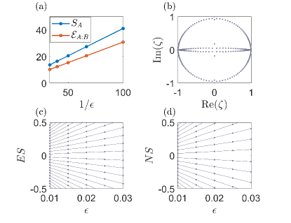
Figure 5: (a) The evolution of $S_{A}$ and negativity $\mathcal{E}_{A:B}$ with different regulator $\epsilon$ at $N_{c}\rightarrow\infty$ limit, in the NS-NS-NS sector for the Majorana fermion. (b) Distribution of the eigenvalues of $\Gamma_{+}$, at $N_{c}=500$ and $\epsilon=0.02$ for the complex fermion. (c,d) Entanglement spectrum and negativity spectrum for $N_{c}=200$ at different $\epsilon$, which shows equal spacing behavior.

Finally, we turn to the reflected entropy and the conjecture (10). We study this difference for the four aforementioned cases and show the results in Fig. 6. For the Majorna and Dirac fermion edge theories in the NS-NS-NS sector, and the Majoran fermion edge theory in the R-R-R sector, $h_{A:B}$ does not change with $\epsilon$, with the values being 0.1172, 0.2344, 0.2850 respectively. The results for the NS-NS-NS sector are consistent with the prediction $(c/3)\ln 2=0.1155,0.2310$ for $c=1/2$ and $c=1$, respectively. (Alternatively, if we extract the central charge from our numerics, we obtain $c=0.5073,1.0145,1.2335$, respectively.) For the R-R-R sector, the numerics suggests that $h_{A:B}$ is slightly bigger than $(c/3)\ln 2$, which once again may be attributed to the Ising anyon at the junction. Finally, for the Dirac fermion in the R-R-R sector, $h_{A:B}$ changes with $\epsilon$ and the polynomial fit up to second order gives the intercept 0.5698. Notice that 0.2344 is twice as large as 0.1172, and 0.5698 is (almost) twice as large as 0.2850. We note that to get the universal result in the edge theory calculations, we do not have to consider a local unitary that remove short-range correlations at the junction(s).

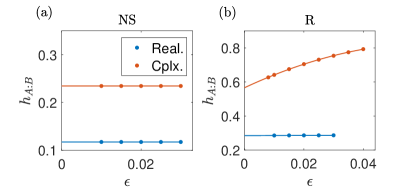
Figure 6: The difference between reflected entropy and mutual information $h_{A:B}=R_{A:B}-I_{A:B}$. (a) The NS-NS-NS sector for Majorana fermion and complex fermion. The intercept (0.2344) is twice of that of the Majorana fermion (0.1172). (b) The R-R-R sector for Majorana fermion and complex fermion. Using a power two polynomial fit, the intercept (0.5698) is almost the twice of that of the Majorana fermion (0.2850). In (a) and the real fermion case of (b), $h_{A:B}$ does not change with $\epsilon$.

V Lattice model approach

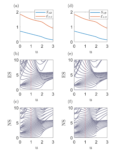
Figure 7: The von Neumann entanglement entropy and logarithmic negativity for the Chern insulator model on a $20\times 20$ lattice ($l=20$) for (a-c) anti-periodic boundary condition and (d-f) periodic boundary condition. The lattice partition is shown in Fig. 1(b) where $l_{A}=10$; both $A$ and $B$ are $10\times 10$ blocks. (a,d) The von Neumann entanglement entropy $S_{AB}$ and logarithmic negativity $\mathcal{E}_{A:B}$. (b,e) Entanglement spectrum $\ln(\frac{2}{1+\gamma}-1)$. $\gamma$ is four-fold degenerate for both topological and trivial region, which is observed for both of the boundary conditions. For the periodic boundary condition (e), there exist four-fold degenerate zero modes. (c,f) Negativity spectrum $\ln(\frac{2}{1+\gamma_{\times}}-1)$. Note at $u=1$, the low lying spectrum shows equal spacing pattern, which is a CFT signature. $\gamma_{\times}$ is 4-fold degenerate in the topological region and becomes 8-fold degenerate in the trivial region, which is observed for both the boundary conditions.

Though the edge theory, or “cut-and-glue” approach provides a theoretically appealing way of computing entanglement measures in the thermodynamic limit, it is limited by the fact that it is only applicable to systems deep in the topological phase. It is natural to ask how the entanglement properties of a system change closer to and across a topological phase transition.

To that end and as a check on the conclusions we have drawn from the edge theory approach, in this section, we study a tight-binding model on the square lattice that realizes a Chern insulator phase. The Hamiltonian is given by

$$H =\frac{-i}{2}\sum_{\bm{r}}\sum_{\mu=x,y}\left[f_{\bm{r}}^{\dagger}\tau_{\mu}f^{\ }_{\bm{r}+\bm{a}_{\mu}}-f_{\bm{r}+\bm{a}_{\mu}}^{\dagger}\tau_{\mu}f^{\ }_{\bm{r}}\right]$$

$$\quad+\frac{1}{2}\sum_{\bm{r}}\sum_{\mu=x,y}\left[f_{\bm{r}}^{\dagger}\tau_{z}f^{\ }_{\bm{r}+\bm{a}_{\mu}}+f^{\dagger}_{\bm{r}+\bm{a}_{\mu}}\tau_{z}f^{\ }_{\bm{r}}\right]$$

$$\quad+u\sum_{\bm{r}}f_{\bm{r}}^{\dagger}\tau_{z}f^{\ }_{\bm{r}},$$ (91)

where the two-dimensional integer vector $\bm{r}$ labels sites on the square lattice, and $\bm{a}_{x}=(1,0)$ and $\bm{a}_{y}=(0,1)$; $f^{{\dagger}}_{\bm{r}}/f^{\ }_{\bm{r}}$ are two-component fermion creation/annihilation operators at site $\bm{r}$, and $\tau_{\mu=x,y,z}$ are the Pauli matrices. In momentum space, the corresponding Bloch Hamiltonian is,

$$h(\mathbf{k})=\sin{k_{x}}\tau_{x}+\sin{k_{y}}\tau_{y}+(u+\cos{k_{x}}+\cos{k_{y}})\tau_{z},$$ (92)

with $k_{x,y}\in[-\pi,\pi]$. The parameter $u$ tunes the model across insulating phases with different Chern numbers: the Chern number ${\it Ch}=0$ for $|u|>2$, ${\it Ch}=1$ for $0<u<2$ and ${\it Ch}=-1$ for $-2<u<0$. The many body ground state $|{\it GS}\rangle$ is obtained by filling the lower band. On an $N\times N$ square lattice, the correlation matrix elements are given by $\langle{\it GS}|f^{\dagger}_{\bm{r},s}f^{\ }_{\bm{r}^{\prime},s^{\prime}}|{\it GS}\rangle={N}^{-1}\sum_{\mathbf{k}}v^{*}_{(\mathbf{k},s,-)}v_{(\mathbf{k},s^{\prime},-)}e^{-i\mathbf{k}\cdot(\bm{r}-\bm{r}^{\prime})}$, where $s=1,2$ and $v_{\mathbf{k},s,-}$ is the $s$-th component of the Bloch eigen vector of the lower band. Since it is a particle number conserving model, the correlation matrix $\Gamma$ is simply given by $\Gamma=(\mathbbm{1}-2C)\otimes\sigma_{y}$.

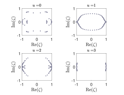
Figure 8: Single-particle spectrum $\{\zeta\}$ of $\rho^{T_{A}}_{A\cup B}$’s correlation matrix $\Gamma_{+}$ for various values of $u$ on $20\times 20$ lattice with anti-PBC. Note that the $\zeta$ spectrum is complex, with real and imaginary parts.

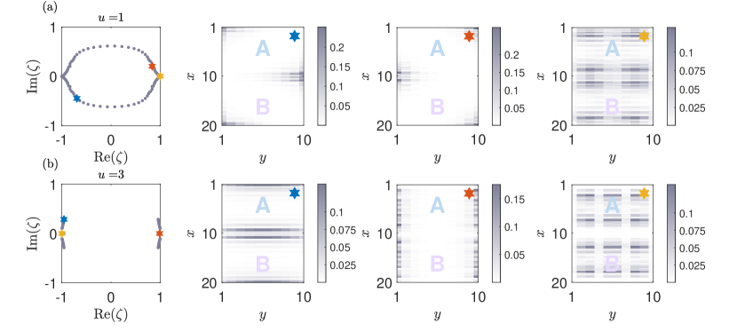
Figure 9: Eigenvectors of $\Gamma_{+}$ at (a) $u=1$ and (b) $u=3$ using anti-PBC for a $20\times 20$ lattice. For each $u$, we take three different eigenvalues, as indicated using the blue, orange and yellow stars, and plot the corresponding eigenvectors supported on $A\cup B$. The eigenvectors exhibit differing patterns of spatial localization for difference phases.

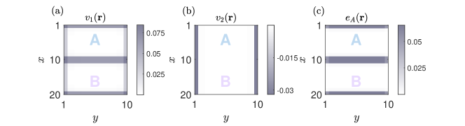
Figure 10: Distribution of (a) $v_{1}(\bm{r})$, (b) $v_{2}(\bm{r})$ and (c) negativity contour $e_{A:B}(\bm{r})$ at $u=1$ for a $20\times 20$ lattice, supported on region $A\cup B$.

We consider tripartitioning the square lattice into three regions $A,B,C$, and trace out the region $C$ (Fig. 1(b)). Since this is a non-interacting system, the reduced density matrix $\rho_{A\cup B}$ is Gaussian. We can then use the correlator method reviewed in Sec. II.1 to construct the partially transposed density matrix $\rho_{A\cup B}^{T_{A}}$. The entanglement spectrum of this model was first studied in Ref. Ryu_2006 .

Entanglement entropy and negativity

The numerically computed entanglement entropy $S_{AB}$ and negativity $\mathcal{E}_{A:B}$, and the corresponding spectra $\{\gamma\}$ and $\{\gamma_{\times}\}$ are shown in Fig. 7. We first verify that both $S_{AB}$ and $\mathcal{E}_{A:B}$ obey area law scaling with the size of lattice $l$, as expected (not shown in the figure). In addition, we see that the phase transition at $u=2$ appears to manifest as a small “bump” in $\mathcal{E}_{A:B}$. A similar though less pronounced change in the slope of $S_{AB}$ as a function of $u$ at $u=2$ is somewhat visible.

Clearer signatures of this phase transition, as well as the topological nature of the phases, are provided by the entanglement and negativity spectra. Indeed, for periodic boundary conditions, both the entanglement spectrum and negativity spectrum exhibit discontinuous behavior at the phase transition point $u=0,\pm 2$ , as we can see in Fig. 7(e,f). For anti-periodic boundary conditions, the spectra are no longer discontinuous across the phase transition. However, the transition still appears to manifest in the spectra by lifting of low lying modes and change in the degeneracy (see the discussion below) when crossing from the topological phase to the trivial phase. The discontinuous behavior also does not exist for more general twisted boundary conditions.

Moving on to the properties of the phases themselves, we see that deep inside the topological phase, around $u=1$ where the bulk gap is the largest, the entanglement spectrum is evenly spaced, at least for the “low-energy” regime. This is consistent with the expectation that the low-energy part of the reduced density matrix is well described by $\rho_{A\cup B}\sim\exp{(-\xi H_{{\it CFT}})}$ where $H_{{\it CFT}}$ is the (physical) CFT Hamiltonian for the edge state, namely the free complex fermion CFT with $c=1$. Here, $\xi$ is a non-universal parameter, controlled by the bulk correlation length, for example. Similarly, around $u=1$, the negativity spectrum is also evenly spaced. This likewise suggests that $\rho_{\times,A\cup B}$ is given by $\rho_{\times,A\cup B}\sim\exp{(-\xi H^{\prime}_{{\it CFT}})}$, where $H^{\prime}_{{\it CFT}}$ is a Hamiltonian of CFT, which may differ from $H_{{\it CFT}}$.

Moreover, the degeneracy of the entanglement and negativity spectra reveal signatures of the two phases and the boundary conditions. One the one hand, every eigenvalue $\gamma$ is four-fold degenerate in the ES for $S_{AB}$ and two-fold degenerate in the ES for $S_{A}$. On the other hand, the negativity spectrum $\gamma_{\times}$ is four-fold degenerate in the topological region and becomes eight-fold degenerate deep in trivial region, which is observed for both of the boundary conditions. We thus see that the degeneracy of the NS provides a signal for the topology of the ground state, in contrast to the ES. The degeneracies deep in the topological region (two-fold for ES and four-fold for NS) match up with the edge theory results presented earlier in Sec. IV.2.

To compare with the results from the conformal field theory calculation, let’s compare the entanglement entropy and logarithmic negativity at $u=1$ for anti-periodic boundary condition (i.e., the N-N-N sector) and periodic boundary condition (i.e., the R-R-R sector).

When taking $AB$ as the subsystem to compute the entanglement entropy, the entanglement spectra for PBC and APBC are different (due to the zero mode), but they give the same entanglement entropy. This is similar to our previous experience in bipartition boundary state, where the NS-NS and R-R sectors give the same entanglement entropy.

When taking $A$ as the subsystem to compute the entanglement entropy, we find the entanglement spectra for $S_{A}$ are the same when deep in the topological region $u=1$, and deep into the trivial region $u=3$. When coming closer to the critical point, these two spectra become different. (We note, in contrast, in the edge theory calculation, the NS-NS-NS and R-R-R sectors give different entanglement entropies, $S_{A}$. The precise reason for the disagreement between the lattice and edge theory calculations is unclear. We however note that the configurations are not exactly the same – for example, there are two junctions in the edge theory calculations whereas there are four junctions in the lattice calculation.)

For negativity spectrum, we also find that the PBC and APBC give the same spectrum $\gamma_{\times}$ at $u=1$. This is only true deep in the topological region. For example, if we take $u=1.9$ or $u=0.1$, we can see the vast difference between the two spectra. Furthermore, when going deep into the trivial region $u=3$, the two spectra become identical again.

Spectrum of $\Gamma_{+}$

We now move on to the numerically obtained spectrum $\{\zeta\}$ of $\Gamma_{+}$, plotted in Figs. (8)-(9), for various $u$ with anti-PBC. We see that they provide clear signatures of the topology of the phase. Indeed, in the Chern insulator phases, the eigenvalues $\{\zeta\}$ are non-trivially distributed over the complex plane. In the trivial insulator phases, on the other hand, the eigenvalues $\{\zeta\}$ are localized near $\zeta=-1;1$. In the atomic limit $u\rightarrow\infty$, we expect that the spectrum collapses to two points $\zeta=-1;1$. The distribution of $\{\zeta\}$ is also non-trivial at the critical points $u=0,\pm 2$. However, we defer the discussions for the critical points, and focus on the Chern insulator phase.

In particular, in the Chern insulator phase, we can identify two types (branches) of eigenvalues, those that are away from the real axis ($\mathrm{Im}(\zeta)\neq 0$); and those that are exactly on $\zeta=-1$ and $\zeta=1$, which are highly degenerate. We believe that the appearance of these states is closely tied to the topological properties of the Chern insulator phase, in the same way that midgap states in the regular entanglement spectrum indicate nontrivial topology.

Moreover, the eigenstates corresponding to these two types of eigenvalues are distinguished by their real space profiles, as shown in Fig. 9. For the first type of eigenvalues, the corresponding eigenstates are localized near the points where the regions $A$, $B$ and $C$ all meet. On the other hand, for the eigenvalues at $\zeta=-1,1$, the eigenstates are distributed throughout the bulk. In contrast, in the trivial phase $u=3$, from Fig. 9, there do not exist eigenstates localized at the intersection of $A,B$ and $C$.

Figure 11: (a) The difference between reflected entropy and mutual information $h_{A:B}=R_{A:B}-I_{A:B}$, computed on $20\times 20$ lattice ($L=20$). (b) Scaling of $h_{A:B}$ with the size of lattice $l$ at $u=1.34$, which shows that $h_{A:B}$ is a constant 2.272. $u=1.34$ is where $h_{A:B}$ is minimal in the topological phase.

Negativity contour

To better understand the spatial decomposition of the negativity, we plot the negativity contour (18) of a $20\times 20$ lattice at $u=1$ (Fig. 10). From (c), the negativity contour is only supported near the boundary between $A$ and $B$, but not the boundary between $AB$ and their complement, which is as expected. From (a)(b), we find this is because adding $v_{1},v_{2}$ together makes the non-zero values on the boundary between $AB$ and their complement cancel.

Reflected entropy

We finally examine the reflected entropy and mutual information, and show their difference $h_{A:B}$ in Fig. 11 (in units of $\ln(2)/3$). As the entanglement entropy and negativity, it is peaked at the phase transitions and takes smaller values in gapped phases. In the ${\it Ch}=1$ phase, $h_{A:B}$ takes its minimum around $u\sim 1.34$ – we focus on this point and test the conjecture (10). There, $h_{A:B}$ is independent of $l$, and $h_{A:B}\sim 2.272\times(c/3)\times\ln 2$ (with $c=1$). We should first note that the setup in the lattice calculations has four junctions where all the three regions meet, whereas in our edge theory calculations there are two junctions [see Fig. 3(a)]. This may result in a factor of two difference between the edge theory and lattice calculations. Even taking into account the difference in the number of junctions, $h_{A:B}$ is not quantized to $(c/3)\ln 2$. We expect this to be a consequence of non-universal contributions coming from the sharp corners at the trijunction. This would suggest that the edge theory approach provides a reliable way of extracting universal topological contributions to the reflected entropy (and other entanglement measures) without being obscured by non-universal and/or geometric effects. Similar to the entanglement entropy, both APBC and PBC give the same result when $u$ is not so close to the critical point. Once again this may be attributed to the different configurations adopted in the edge theory and lattice calculations.

VI Conclusion

We have investigated correlation measures, i.e., entanglement entropy, entanglement negativity, and reflected entropy, in the ground states of topological liquid in (2+1) dimensions, in the multipartition setting (Fig. 1). This was done by constructing vertex states explicitly in various configurations with or without fluxes.

In the bipartition case, we study the entanglement entropy in the NS-NS, R-R, and NS-R sectors, and unveil a new topological contribution in the NS-R case. This contribution is due to the non-trivial configuration where a $\sigma$-anyon exits from the entanglement cut.

In the tripartition case, we find the correlation measures capture various universal characteristics of topological liquids. For example, we found that the spectrum of the partially transposed density matrix is non-trivially distributed over the complex plane. This is somewhat similar to the spectrum previously computed for (1+1)d fermionic conformal field theory and symmetry-protected topological phases. There, a non-trivial dependence of the spectrum on the spin structures was observed shapourian2019twisted ; inamura2020non . We also found universal topological contribution to negativity and $h_{A:B}$. In the NS-NS-NS case, we verified the conjecture (10) for the reflected entropy, while there exists an additional contribution to $h_{A:B}$ in the R-R-R sector due to the $\sigma$-anyon.

There are a number of open questions to be discussed. First of all, our tripartition setup is different from the ones considered previously (except for the original Kitaev-Preskill setup kitaev2006topological ), and more complicated in the sense that the entangling boundaries are not smooth, but have a singular point where all spatial regions meet. One may wonder if the correlation measures depend not just on topological but also on geometrical properties of entangling boundaries. For example, entanglement entropy is known to have a non-trivial corner contribution when the entangling boundary has a sharp corner in critical theories Hirata_2007 ; kallin2013 ; Kallin_2014 ; Bueno_2015 ; Faulkner_2016 ; Bueno_2016 ; Whitsitt_2017 ; Seminara_2017 ; Bueno_2019 ; Stoudenmire2014 ; similar behavior was recently found in the context of integer quantum Hall states Sirois2021 . One could imagine that there is a similar contribution to quantities that we studied in our work. It is unclear at this moment if our method is capable of capturing non-trivial geometry at the point where all spatial regions meet. Also, as we mentioned, in the R-R-R sector, we expect that a non-trivial flux (anyon) should be located just at the junction because of the conservation of topological charge. Understanding how precisely correlation measures depend on such excitation is an important open question.

Putting our work in a slightly broader context, one of the important questions is to understand what kind of underlying (topological/geometrical) data can appear in entanglement measures. While we took chiral $p$-wave superconductors and Chern insulators as examples, in order to get more general pictures, it is desirable to extend our analysis to more generic topological liquids. In the future, we plan to study Abelian fractional quantum Hall states by constructing vertex states for multi-component compactified boson theories. We can also discuss cases where the different spatial regions $A,B,C$ have different topological orders. Such configurations involving gapped interfaces between distinct phases have garnered much attention recently due to the possibility of trapping parafermion zero modes at domain walls along these interfaces BarkeshliQi-2012 ; Lindner-2012 ; Clarke-2013 ; Cheng-2012 ; BarkeshliJianQi-2013-a ; BarkeshliJianQi-2013-b ; Mong-2014 ; khanteohughes-2014 ; SantosHughes-2017 ; santos2019 . The entanglement entropy for an interface between two distinct arbitrary Abelian phases cano2015interfaces ; fliss2017interface and for particular classes of non-Abelian phases fliss2020nonabelianinterface ; sohal2020nonabelian has already been computed. In the former case, the entanglement was subsequently shown to signal the presence of an emergent one-dimensional topological phase along the interface Santos2018 . It is natural to expect more exotic outcomes could occur in the trijunction configurations we have considered.

Finally, while we took in this paper an approach from the edge theory, it is interesting to study the entanglement negativity using complementary bulk approaches. For example, we can study entanglement negativity in lattice models such as string net models. Also, it is interesting to formulate surgery calculations for the entanglement measures we have considered witten1989jones ; dong2008surgery ; wen2016surgery ; fliss2020nonabelianinterface ; berthiere2021 . These alternative bulk calculations can clarify precisely what kind of topological data can be captured by the entanglement negativity in the setup studied in this work.

Appendix A Direct calculation method

The Neumann function method provides an elegant way of deriving the form of the conformal boundary state for free theories, which extends straightforwardly to the tripartition case (and, indeed, more general $n$-partition). As a check on our results using this method, we rederive the vertex states in this section using a more direct approach. In this section, we will work with the Majorana and complex fermion fields.

We recall that the edge state Hamiltonian including gapping potential terms is given by

$$H_{0} =\int_{0}^{2\pi}d\sigma\sum_{I}f^{I{\dagger}}i\partial_{\sigma}f^{I},$$

$$H_{{\it int}} =\int_{0}^{2\pi}d\sigma\bm{f}^{{\dagger}}(\sigma)M\bm{f}(2\pi-\sigma)+{\it h.c.}$$ (93)

where in the last line we used a vectorial notation and the mass matrix $M$ is given by

$$M=m\left(\begin{array}[]{ccc}0&1&0\\ 0&0&1\\ 1&0&0\end{array}\right).$$ (97)

Corresponding to this situation, we seek for a state $|V\rangle$ which satisfies, for $0<\sigma<\pi$,

$$\left[f^{I}(\sigma)-if^{I+1}(2\pi-\sigma)\right]|V\rangle=0.$$ (98)

Solving the constraint, the state $|V\rangle$ is given in the form of a fermionic coherent state. A major simplification for the case of complex fermion is that we can diagonalize the mass matrix $M$ by a unitary rotation $U$ as $M=U^{\dagger}\Lambda U$, where

$$U=\frac{1}{\sqrt{3}}\left(\begin{array}[]{ccc}1&1&1\\ \omega^{*}&\omega&1\\ \omega&\omega^{*}&1\end{array}\right),$$ (102)

$$\Lambda=\mathrm{diag}(1,\omega,\omega^{*}),\quad\omega=e^{2\pi i/3}.$$ (103)

In the rotated basis $\bm{\eta}:=U\bm{f}$, the edge Hamiltonian is diagonal and given by

$$H_{0}=\int_{0}^{2\pi}d\sigma\sum_{a=1}^{3}\eta^{\dagger}_{a}i\partial_{\sigma}\eta^{\ }_{a},$$

$$H_{int}=\int_{0}^{\pi}d\sigma\sum_{a=1}^{3}me^{i\theta_{a}}\eta_{a}^{\dagger}(\sigma)\eta^{\ }_{a}(2\pi-\sigma),$$ (104)

where $\theta_{1}=0$, $\theta_{2}=2\pi/3$, and $\theta_{3}=-2\pi/3$. We take the spatial boundary conditions (Ramond or Neveu-Schwarz) for $I=1,2,3$ being all identical, so the rotation does not affect the spatial boundary condition. Thus, in the rotated basis, we have three copies of the single fermion problem,

$$\left[\eta_{a}(\sigma)+g_{a}(\sigma)\eta_{a}(2\pi-\sigma)\right]|V\rangle=0,$$

$$\mbox{where}\quad g_{a}(\sigma)=-is(\sigma)e^{is(\sigma)\theta_{a}},$$ (105)

and $s(\sigma)$ is the sign function: $s(\sigma)=1$ for $0<\sigma<\pi$ and $s(\sigma)=-1$ for $\pi<\sigma<2\pi$. Similarly, the boundary condition for $\eta^{\dagger}$ is given by

$$\left[\eta^{{\dagger}}_{a}(\sigma)+\tilde{g}_{a}(\sigma)\eta^{{\dagger}}_{a}(2\pi-\sigma)\right]|V\rangle=0$$

$$\mathrm{where}\quad\tilde{g}_{a}(\sigma)\equiv-g_{a}(-\sigma)=-is(\sigma)e^{-is(\sigma)\theta_{a}}.$$ (106)

For now, we focus on the vertex state for a given copy and omit the subscript $a$. We will restore the subscript later when it is necessary. By mode expansion, $\eta(\sigma)=\sum_{r}e^{-i\sigma r}\eta_{r}$ and $g(\sigma)=\sum_{n\in\mathbb{Z}}e^{in\sigma}g_{n}$, the gluing condition can be written as

$$[\eta_{r}+N_{r,s}\eta_{s}]|V\rangle=0,$$ (107)

where $N_{r,s}:=g_{-r-s}$ and the Fourier components of $g(\sigma)$ are given by

$$g_{n} =\begin{cases}0&n\neq 0\text{, $n$ is even}\\ \frac{-2\cos{\theta}}{n\pi}&\text{$n$ is odd}\\ \sin{\theta}&n=0\end{cases}.$$ (108)

In the next subsections, we discuss the construction of the vertex state for each copy, for the Majorana and Dirac fermion fields separately. Here, we summarize the result. We separate $N_{r,s}$ into four blocks,

$$N^{++}_{r,s}=N_{r,s},\quad N^{--}_{r,s}=N_{-r,-s},\quad$$

$$N^{-+}_{r,s}=N_{-r,s},\quad N^{+-}_{r,s}=N_{r,-s},\quad r,s>0$$ (109)

The vertex state solution is

$$|V\rangle\propto\exp\Big{(}\sum_{r,s\geq 1/2}K_{rs}\eta^{\dagger}_{r}\eta^{\ }_{-s}\Big{)}|0\rangle,$$

$$\mathrm{with}\quad K\equiv-(\mathbbm{1}+N^{++})^{-1}(N^{+-})$$

$$\hskip 38.41139pt=-(N^{-+})^{-1}(\mathbbm{1}+N^{--}),$$ (110)

where $|0\rangle$ is the Fermi sea annihilated by $\eta_{r},r>0$ and $\eta_{r}^{\dagger},r<0$. The equivalence of the two expressions of $K$ comes from the fact that $\sum_{s}N_{rs}N_{st}=\delta_{r,t}$. We give the detailed derivation in the next subsections. Denoting $\eta_{r}=u_{r}$ and $\eta_{-r}=v_{r}^{\dagger}$ for $r>0$, the solution can be written in the familiar Gaussian state form,

$$|V\rangle \propto\exp{\Big{(}\sum_{r,s\geq 1/2}K_{rs}u^{\dagger}_{r}v^{\dagger}_{s}\Big{)}}|0\rangle$$

$$=\exp{\Big{(}\frac{1}{2}\sum_{r,s\geq 1/2}\left[K_{rs}u^{\dagger}_{r}v^{\dagger}_{s}-(K^{T})_{rs}v_{r}^{\dagger}u_{s}^{\dagger}\right]\Big{)}}|0\rangle.$$ (111)

Combinining the three copies $\eta_{1},\eta_{2},\eta_{3}$ and restoring the subscript $a=1,2,3$ for $K,u,v$, the vertex state in the rotated basis is

$$|V\rangle=\mathcal{N}\exp{\left[\frac{1}{2}(\bm{V}^{\dagger})^{T}\bm{K}\bm{V}^{\dagger}\right]}|0\rangle$$ (112)

where

$$(\bm{V}^{\dagger})^{T}=\left(\bm{u}_{1}^{\dagger},\bm{v}_{1}^{\dagger},\bm{u}_{2}^{\dagger},\bm{v}_{2}^{\dagger},\bm{u}_{3}^{\dagger},\bm{v}_{3}^{\dagger}\right),$$

$$\bm{K}=\left(\begin{array}[]{cccccc}0&K_{1}&0&0&0&0\\ -K_{1}^{T}&0&0&0&0&0\\ 0&0&0&K_{2}&0&0\\ 0&0&-K_{2}^{T}&0&0&0\\ 0&0&0&0&0&K_{3}\\ 0&0&0&0&-K_{3}^{T}&0\\ \end{array}\right).$$ (119)

We may use an inverse rotation to write the solution in the original basis $f,f^{\dagger}$ (See Appendix A.3).

A.1 Majorana fermion

Let us now discuss the type of state presented in (105) and (106) in more detail. As a warm up, we first consider a similar problem for the Majorana fermion edge mode, following Ref. imamura2008boundary . Let us consider the Majorana fermion field, and the boundary condition

$$\big{[}\psi(\sigma)+g(\sigma)\psi(-\sigma)\big{]}|V\rangle=0\quad\mathrm{for}\quad-\pi<\sigma<\pi.$$ (120)

We focus on the NS sector. As a specific example, we can take $g(\sigma)=\pm i\mathrm{sign}(\sigma)$. We however proceed with a generic choice of $g(\sigma)$. $g(\sigma)$ is subject to a consistency condition: Assuming $g(\sigma)\neq 0$, we note that the condition (120) can be rewritten as

$$\big{[}g(\sigma)^{-1}\psi(\sigma)+\psi(-\sigma)\big{]}|V\rangle=0$$

$$\Longrightarrow\big{[}g(-\sigma)^{-1}\psi(-\sigma)+\psi(\sigma)\big{]}|V\rangle=0.$$ (121)

Comparison with Eq. (120) implies

$$g(\sigma)g(-\sigma)=1.$$ (122)

In terms of the Fourier components of $g(\sigma)$, $g(\sigma)=\sum_{n\in\mathbb{Z}}e^{in\sigma}g_{n},$ the consistency condition reads $\sum_{n}g_{n}g_{n+p}=\delta_{p,0}.$

Let us now proceed to the construction of $|V\rangle$. Defining a matrix $N_{n,m}=g_{-n-m}$, the boundary condition and the consistency relation can be written as

$$\big{[}\psi_{r}+\sum_{s}N_{r,s}\psi_{s}\big{]}|V\rangle=0,$$

$$\sum_{m}N_{n,m}N_{m,l}=\delta_{nl}\quad(N^{2}=\mathbbm{1}),$$ (123)

respectively. For convenience, we use fermionic creation/annihilation operators to write

$$\left(\begin{array}[]{c}\psi_{1/2}\\ \psi_{3/2}\\ \vdots\end{array}\right)\equiv\bm{b},\quad\left(\begin{array}[]{c}\psi_{-1/2}\\ \psi_{-3/2}\\ \vdots\end{array}\right)\equiv\bm{b}^{\dagger}.$$ (124)

We also introduce a block structure

$$N=\left(\begin{array}[]{cc}N^{++}&N^{+-}\\ N^{-+}&N^{--}\end{array}\right),$$ (127)

$$N^{++}_{r,s}=N_{r,s}=g_{-r-s},\quad N^{+-}_{r,s}=N_{r,-s}=g_{-r+s},$$

$$N^{-+}_{r,s}=N_{-r,s}=g_{r-s},\quad N^{--}_{r,s}=N_{-r,-s}=g_{r+s}.$$

From the consistency condition $N^{2}=\mathbbm{1}$, these blocks satisfy

$$(i) \quad N^{++}N^{++}+N^{+-}N^{-+}=\mathbbm{1},$$

$$(ii) \quad N^{++}N^{+-}+N^{+-}N^{--}=0,$$

$$(iii) \quad N^{-+}N^{++}+N^{--}N^{-+}=0,$$

$$(iv) \quad N^{-+}N^{+-}+N^{--}N^{--}=\mathbbm{1}.$$ (128)

We also note $N^{T}=N$, which is the consequence of $N_{r,s}=g_{-r-s}$. This leads to

$$(N^{++})^{T}=N^{++},\quad(N^{--})^{T}=N^{--},$$

$$(N^{+-})^{T}=N^{-+},\quad(N^{-+})^{T}=N^{+-}.$$ (129)

The boundary condition (A.1) can now be written two different ways as

$$\big{[}\psi_{r}+\sum_{s>0}N_{r,s}\psi_{s}+\sum_{s>0}N_{r,-s}\psi_{-s}\big{]}|V\rangle=0$$

$$\quad\Longrightarrow\begin{cases}\big{[}\bm{b}+(\mathbbm{1}+N^{++})^{-1}N^{+-}\bm{b}^{\dagger}\big{]}|V\rangle=0\\ \big{[}\bm{b}+(N^{-+})^{-1}(\mathbbm{1}+N^{--})\bm{b}^{\dagger}\big{]}|V\rangle=0.\end{cases}$$ (130)

The equivalence of the two conditions can be established by using the consistency equations $(i)-(iv)$: We first note that

$$(\mathbbm{1}+N^{++})(\mathbbm{1}-N^{++})=\mathbbm{1}-(N^{++})^{2}=N^{+-}N^{-+}$$ (131)

where we used $(i)$ in the first line. This relation can be rewritten as

$$(\mathbbm{1}-N^{++})^{-1}(\mathbbm{1}+N^{++})^{-1}=(N^{+-}N^{-+})^{-1}$$ (132)

$$\quad\Longrightarrow\quad(\mathbbm{1}+N^{++})^{-1}(N^{+-})=(\mathbbm{1}-N^{++})(N^{-+})^{-1}.$$

Next, from $(iii)$, we note that $N^{-+}$ intertwines the $+$ and $-$ sectors as $N^{-+}N^{++}=-N^{--}N^{-+}$. This leads to $N^{++}(N^{-+})^{-1}=-(N^{-+})^{-1}N^{--}$, and $(N^{++})^{k}(N^{-+})^{-1}=(N^{-+})^{-1}(-N^{--})^{k}$. Then,

$$(\mathbbm{1}-N^{++})(N^{-+})^{-1}=(N^{-+})^{-1}(\mathbbm{1}+N^{--}),$$ (133)

which completes the proof of the equivalence. We now define

$$K:=(\mathbbm{1}+N^{++})^{-1}(N^{+-})=(N^{-+})^{-1}(\mathbbm{1}+N^{--}),$$ (134)

and write the boundary condition as

$$\left[\bm{b}+K\bm{b}^{\dagger}\right]|V\rangle=0.$$ (135)

We note that if $g(\sigma)$ is odd under $\sigma\to-\sigma$, $g_{n}=-g_{-n}$, then $K^{T}=-K$. This can be seen by first noting that $g_{n}=-g_{-n}$, implies $N^{++}=-N^{--}$ and $N^{+-}=-N^{-+}$, which make $N^{++}/N^{--}$ and $N^{+-}/N^{-+}$ commute. We then see

$$K^{T} =(N^{+-})^{T}[(\mathbbm{1}+N^{++})^{-1}]^{T}$$ (136)

$$=(N^{-+})(\mathbbm{1}+N^{++})^{-1}$$

$$=(\mathbbm{1}+N^{++})^{-1}(N^{-+})$$

$$=(\mathbbm{1}+N^{++})^{-1}(-N^{+-})=-K.$$

Finally, using the antisymmetry of $K$, we can write down the solution of boundary condition $\left[\bm{b}+K\bm{b}^{\dagger}\right]|V\rangle=0$:

$$|V\rangle\propto\exp{\Big{(}-\frac{1}{2}\sum_{r,s\geq 1/2}K_{r,s}b_{r}^{\dagger}b_{s}^{\dagger}\Big{)}}|0\rangle.$$ (137)

This can be checked by the Baker-Hausdorff formula.

A.2 Dirac fermion

Let us now turn to the case of Dirac fermions $f(\sigma),f^{{\dagger}}(\sigma)$. Consider a boundary condition

$$[f(\sigma)+g(\sigma)f(-\sigma)]|V\rangle=0,$$

$$[f^{\dagger}(\sigma)+\tilde{g}(\sigma)f^{\dagger}(-\sigma)]|V\rangle=0,$$ (138)

for $-\pi<\sigma<\pi$. At this moment, $\tilde{g}(\sigma)$ appears to be an independent function, not related to $g(\sigma)$. We however require the condition

$$\tilde{g}(\sigma)=-g(-\sigma).$$ (139)

We will see momentarily the implication of this condition on the vertex state. As a specific example, we consider

$$g(\sigma)=-is(\sigma)e^{is(\sigma)\theta},$$

$$\tilde{g}(\sigma)=-g(-\sigma)=-is(\sigma)e^{-is(\sigma)\theta},$$ (140)

where $s(\sigma)=\mathrm{sgn}(\sigma)$.

In the Fourier space, the condition (A.2) reads

$$\big{[}f_{r}+\sum_{s}N_{r,s}f_{s}\big{]}|V\rangle=0,$$

$$\big{[}\tilde{f}_{r}+\sum_{s}\tilde{N}_{r,s}\tilde{f}_{s}\big{]}|V\rangle=0,$$

$$N_{r,s}=g_{-r-s},\quad g(\sigma)=\sum_{n\in\mathbb{Z}}e^{in\sigma}g_{n}.$$

$$\tilde{N}_{r,s}=\tilde{g}_{-r-s},\quad\tilde{g}(\sigma)=\sum_{n\in\mathbb{Z}}e^{in\sigma}\tilde{g}_{n}.$$ (141)

where the Fourier decomposition of $f^{{\dagger}}$ is given by $f^{\dagger}(\sigma)=\sum_{s\in\mathbb{Z}+1/2}e^{i\sigma s}f_{s}^{\dagger}=\sum_{s\in\mathbb{Z}+1/2}e^{-i\sigma s}\tilde{f}_{s}$. Namely, we introduced the new set of operators $\tilde{f}_{s}$ by $\tilde{f}_{s}\equiv f_{-s}^{\dagger}$. Similarly the condition (139) in the Fourier space is

$$\tilde{g}_{n}=-g_{-n}.$$ (142)

We define the creation/annihilated operators as

$$\left(\begin{array}[]{c}f_{1/2}\\ f_{3/2}\\ \vdots\end{array}\right)\equiv\bm{b},\quad\left(\begin{array}[]{c}f_{-1/2}\\ f_{-3/2}\\ \vdots\end{array}\right)\equiv\bm{c}^{\dagger},$$ (149)

$$\left(\begin{array}[]{c}f_{1/2}^{\dagger}\\ f_{3/2}^{\dagger}\\ \vdots\end{array}\right)\equiv\bm{b}^{\dagger},\quad\left(\begin{array}[]{c}f_{-1/2}^{\dagger}\\ f_{-3/2}^{\dagger}\\ \vdots\end{array}\right)\equiv\bm{c},$$ (156)

and we also define, similarly,

$$\left(\begin{array}[]{c}\tilde{f}_{1/2}\\ \tilde{f}_{3/2}\\ \vdots\end{array}\right)\equiv\bm{c},\quad\left(\begin{array}[]{c}\tilde{f}_{-1/2}\\ \tilde{f}_{-3/2}\\ \vdots\end{array}\right)\equiv\bm{b}^{\dagger}.$$ (163)

The conditions in (A.2) can be organized as

$$\big{[}f_{r}+\sum_{s\geq 1/2}N_{r,s}f_{s}+\sum_{s\geq 1/2}N_{r,-s}f_{-s}\big{]}|V\rangle=0$$ (164)

$$\quad\Longrightarrow\begin{cases}\big{[}\bm{b}+(\mathbbm{1}+N^{++})^{-1}N^{+-}\bm{c}^{\dagger}\big{]}|V\rangle=0\\ \big{[}\bm{b}+(N^{-+})^{-1}(\mathbbm{1}+N^{--})\bm{c}^{\dagger}\big{]}|V\rangle=0\end{cases}$$

$$\big{[}\tilde{f}_{r}+\sum_{s\geq 1/2}\tilde{N}_{r,s}\tilde{f}_{s}+\sum_{s\geq 1/2}\tilde{N}_{r,-s}\tilde{f}_{-s}\big{]}|V\rangle=0$$ (165)

$$\quad\Longrightarrow\begin{cases}\big{[}\bm{c}+(\mathbbm{1}+\tilde{N}^{++})^{-1}\tilde{N}^{+-}\bm{b}^{\dagger}\big{]}|V\rangle=0\\ \big{[}\bm{c}+(\tilde{N}^{-+})^{-1}(\mathbbm{1}+\tilde{N}^{--})\bm{b}^{\dagger}\big{]}|V\rangle=0\end{cases}$$

As we have seen, the two conditions in (164) are equivalent by using $N^{2}=\mathbbm{I}$. Similarly, the two conditions in (165) are equivalent by using $\tilde{N}^{2}=\mathbbm{I}$.

Now let us define

$$K =(\mathbbm{1}+N^{++})^{-1}(N^{+-})=(N^{-+})^{-1}(\mathbbm{1}+N^{--}),$$

$$\tilde{K} =(\mathbbm{1}+\tilde{N}^{++})^{-1}(\tilde{N}^{+-})=(\tilde{N}^{-+})^{-1}(\mathbbm{1}+\tilde{N}^{--}).$$ (166)

Then, the boundary conditions are written as $\big{[}\bm{b}+K\bm{c}^{\dagger}\big{]}|V\rangle=\big{[}\bm{c}+\tilde{K}\bm{b}^{\dagger}\big{]}|V\rangle=0$, or

$$\left[\left(\begin{array}[]{c}\bm{b}\\ \bm{c}\end{array}\right)+\left(\begin{array}[]{cc}0&K\\ \tilde{K}&0\end{array}\right)\left(\begin{array}[]{c}\bm{b}^{\dagger}\\ \bm{c}^{\dagger}\end{array}\right)\right]|V\rangle=0.$$ (167)

Here, we note that the condition (139) imposes

$$K^{T}=-\tilde{K}.$$ (168)

This can be seen by first noting

$$K^{T}=(N^{-+})(\mathbbm{1}+N^{++})^{-1}=(\mathbbm{1}-N^{--})^{-1}(N^{-+})$$ (169)

where we use the intertwining relation $N^{-+}N^{++}=-N^{--}N^{-+}$. Second, (139) implies $\tilde{N}^{++}=-N^{--}$, and $\tilde{N}^{+-}=-N^{-+}$, which leads to $K^{T}=(\mathbbm{1}-N^{--})^{-1}(N^{-+})=-(\mathbbm{1}+\tilde{N}^{++})^{-1}(\tilde{N}^{+-})=-\tilde{K}$.

With this condition, the vertex state is given by

$$|V\rangle \propto\exp{\left[-\frac{1}{2}\sum_{r,s\geq 1/2}\left(K_{rs}b_{r}^{\dagger}c_{s}^{\dagger}+\tilde{K}_{rs}c_{r}^{\dagger}b_{s}^{\dagger}\right)\right]}|0\rangle$$ (170)

$$=\exp{\left[-\sum_{r,s\geq 1/2}K_{rs}b_{r}^{\dagger}c_{s}^{\dagger}\right]}|0\rangle$$

$$=\exp{\left[-\sum_{r,s\geq 1/2}K_{rs}f_{r}^{\dagger}f_{-s}\right]}|0\rangle$$

A.3 Comparison with the Neumann function method

Let us now take the complex fermion as an example and compare the elements of the Neumann coefficient matrix $K$ in the NS-NS-NS sector, between the direct calculation and Neumann function method. For the direct calculation method, the matrix $K$ in Eq. (110) is in the rotated $\eta$ basis, so we need to rotate back to $f$ basis, namely,

$$K_{f}=U^{\dagger}\left(\begin{array}[]{ccc}K_{\eta,1}&&\\ &K_{\eta,2}&\\ &&K_{\eta,3}\end{array}\right)U$$ (171)

In the direction method, we take the cutoff to be $N_{c}=400$ and compute the Neumann coefficients $K$ numerically. In the following tables, we take the first $8\times 8$ block from the $K^{12}$ matrix in both cases. The real and imaginary parts obtained from the direct calculation and Neumann function method are:

$$\mathrm{Re}\left[K\right]_{direct}=-\left(\begin{array}[]{cccccccc}0&0.2971&0&0.0945&0&0.0564&0&0.0406\\ -0.2964&0&0.3127&0&0.0990&0&0.0569&0\\ 0&-0.3124&0&0.3183&0&0.1047&0&0.0620\\ -0.0934&0&-0.3178&0&0.3163&0&0.1033&0\\ 0&-0.0988&0&-0.3159&0&0.3189&0&0.1060\\ -0.0549&0&-0.1040&0&-0.3184&0&0.3172&0\\ 0&-0.0568&0&-0.1030&0&-0.3168&0&0.3190\\ -0.0389&0&-0.0612&0&-0.1054&0&-0.3185&0\end{array}\right),$$ (172)

$$\mathrm{Re}\left[K\right]_{Neumann}=\left(\begin{array}[]{cccccccc}0&0.2963&0&0.0933&0&0.0548&0&0.0388\\ -0.2963&0&0.3128&0&0.0990&0&0.0570&0\\ 0&-0.3128&0&0.3177&0&0.1040&0&0.0611\\ -0.0933&0&-0.3177&0&0.3163&0&0.1034&0\\ 0&-0.0990&0&-0.3163&0&0.3184&0&0.1053\\ -0.0548&0&-0.1040&0&-0.3184&0&0.3173&0\\ 0&-0.0570&0&-0.1034&0&-0.3173&0&0.3184\\ -0.0388&0&-0.0611&0&-0.1052&0&-0.3184&0\end{array}\right),$$ (173)

$$\mathrm{Im}\left[K\right]_{direct}=\left(\begin{array}[]{cccccccc}-0.7699&0&-0.0998&0&-0.0638&0&-0.0477&0\\ 0&-0.5703&0&-0.0444&0&-0.0330&0&-0.0265\\ -0.0999&0&-0.5537&0&-0.0384&0&-0.0302&0\\ 0&-0.0444&0&-0.5322&0&-0.0255&0&-0.0212\\ -0.0639&0&-0.0384&0&-0.5291&0&-0.0238&0\\ 0&-0.0330&0&-0.0255&0&-0.5210&0&-0.0179\\ -0.0478&0&-0.0303&0&-0.0238&0&-0.5199&0\\ 0&-0.0265&0&-0.0212&0&-0.0179&0&-0.5156\end{array}\right),$$ (174)

$$\mathrm{Im}\left[K\right]_{Neumann}=-\left(\begin{array}[]{cccccccc}-0.7698&0&-0.0998&0&-0.0638&0&-0.0476&0\\ 0&-0.5702&0&-0.0444&0&-0.0329&0&-0.0264\\ -0.0998&0&-0.5536&0&-0.0383&0&-0.0302&0\\ 0&-0.0444&0&-0.5321&0&-0.0254&0&-0.0211\\ -0.0638&0&-0.0383&0&-0.5291&0&-0.0237&0\\ 0&-0.0329&0&-0.0254&0&-0.5209&0&-0.0178\\ -0.0476&0&-0.0302&0&-0.0237&0&-0.5199&0\\ 0&-0.0264&0&-0.0211&0&-0.0178&0&-0.5155\end{array}\right).$$ (175)

We see these two set of matrices are almost identical (up to a minus sign, which is presumably due to convention). The numerical check for other blocks $K^{11}$, etc shows the same results.

We also compare the $K$ matrices of closed string real fermion using direct calculation and Neumann coefficient method, and arrives at the same conclusion. Note that in the direct calculation, the rotation becomes

$$K_{f}=U^{T}\left(\begin{array}[]{ccc}K_{1,\eta}/2&0&0\\ 0&0&-K_{2,\eta}^{T}/2\\ 0&K_{2,\eta}/2&0\end{array}\right)U.$$ (176)

Appendix B Details of the Neumann coefficient method

In this Section, we give some technical details for the Neumann coefficient method.

B.1 Different choice of the branch cuts in the R-R sector

For the vertex state for bipartition in the R-R sector, we can work alternatively with the following choice of the $g^{IJ}$ function:

$$g^{IJ}_{\sigma-\sigma}=\frac{1}{2}\left[\sqrt{\frac{(\omega-\omega_{1,0})(\omega-\omega_{2,0})}{(\omega^{\prime}-\omega_{1,0})(\omega^{\prime}-\omega_{2,0})}}+(\omega\leftrightarrow\omega^{\prime})\right].$$ (177)

Both choices lead to the same vertex state as we demonstrate below. The choice we made in the main text is somewhat simpler, while this choice here is closer to the branch cuts we choose in our calculations in the R-R-R sectors for tripartition. Using $\omega_{I}=\omega_{I,0}(\frac{1+z}{1-z})$, and $\omega_{1,0}=i,\omega_{2,0}=-i$, the Neumann function is given by

$$R^{11}=R^{22} =\frac{\sqrt{zz^{\prime}}}{z-z^{\prime}}\frac{1}{2}\left[\sqrt{\frac{z}{z^{\prime}}}\frac{1-z^{\prime}}{1-z}+\sqrt{\frac{z^{\prime}}{z}}\frac{1-z}{1-z^{\prime}}\right]=\sum_{m\geq 1}\left(\frac{z^{\prime}}{z}\right)^{m}+\frac{1}{2}\left[\sum_{n\geq 0}z^{n}-\sum_{n\geq 1}(z^{\prime})^{n}\right],$$ (178)

$$R^{12}=-R^{21} =\frac{i\sqrt{zz^{\prime}}}{1-zz^{\prime}}\frac{1}{2}\left[\sqrt{\frac{z}{z^{\prime}}}\frac{1-z^{\prime}}{1-z}+\sqrt{\frac{z^{\prime}}{z}}\frac{1-z}{1-z^{\prime}}\right]=(-i)\sum_{m>0}(zz^{\prime})^{m}+\frac{i}{2}\left[\sum_{n>0}z^{n}+\sum_{n>0}(z^{\prime})^{n}\right].$$

We note that we obtain the desired singular term $\sum_{m\geq 1}(z^{\prime}/z)^{m}=\sum_{m\geq 1}e^{-im(\sigma-\sigma^{\prime})}$ in $R^{11}$ and $R^{22}$. From the expansion coefficients and use the same ansatz solution in Eq. (86), we obtain the vertex state:

$$|V\rangle=\exp\left[-i\sum_{n\geq 1}\chi_{-n}^{1}\chi_{-n}^{2}+\sum_{n\geq 1}\left(\chi_{-n}^{1}\chi_{0}^{1}+\chi_{-n}^{2}\chi_{0}^{2}+i\chi_{-n}^{1}\chi_{0}^{2}-i\chi_{-n}^{2}\chi_{0}^{1}\right)\right]|\Omega\rangle.$$ (179)

This is the same solution as Eq. (57) with the additional requirement $(\chi_{0}^{1}+i\chi_{0}^{2})|\Omega\rangle=0$. Similarly, for the Dirac fermion field in the R-R sector, one can show the solutions from the two choices of the branch cuts also match.

B.2 Verification of the boundary condition in the R sector

In this subsection, we verify that the R-R-R sector vertex state ansatz satisfies the boundary condition for real and complex fermion. The verification for the NS-R two-string solution simply parallels the proof belowjevicki1988supersymmetry , which we shall omit.

For the Majorana fermion case, the ansatz solution is:

$$|V\rangle =\exp\left[\frac{1}{2}\sum_{m,n\geq 1}\chi_{-m}^{I}R^{IJ}_{mn}\chi_{-n}^{J}+2\sum_{m,n\geq 1}\chi_{-m}^{I}R^{IJ}_{m0}\chi_{0}^{J}\right]|\Omega\rangle.$$ (180)

Let us denote $A=\sum_{m,n\geq 1}\frac{1}{2}\chi_{-m}^{I}R^{IJ}_{mn}\chi_{-n}^{J}+\sum_{m\geq 1}2\chi_{-m}^{I}R^{IJ}_{m0}\chi_{0}^{J}$. To show explicitly that this state satisfies the boundary condition, we define

$$D^{I}=\sum_{m\geq 1}2\chi_{-m}^{J}R_{m0}^{JI}.$$ (181)

Using

$$\chi_{p}^{I}|V\rangle=\sum_{n\geq 1}R^{IJ}_{pn}\chi_{-n}^{J}|V\rangle+\exp{(A)}\left[2R^{IJ}_{p0}(\chi_{0}^{J}-\sum_{m\geq 1}\chi_{-m}^{K}R^{KJ}_{m0})\right]|\Omega\rangle,$$ (182)

$$\chi_{0}^{I}|V\rangle=\exp{(A)}\left[\chi_{0}^{I}-\sum_{m\geq 1}2\chi_{-m}^{J}R_{m0}^{JI}\right]|\Omega\rangle,$$

one can check the following relation:

$$\chi^{I}(\sigma)|V\rangle =\sum_{p\geq 1}\chi_{p}^{I}e^{-ip\sigma}|V\rangle+\chi_{0}^{I}|V\rangle+\sum_{p\geq 1}\chi_{-p}^{I}e^{ip\sigma}|V\rangle$$ (183)

$$=\sum_{p,n\geq 1}e^{-ip\sigma}R^{IJ}_{pn}\chi_{-n}^{J}|V\rangle+\sum_{p\geq 1}e^{-ip\sigma}\exp{(A)}\left[2R^{IJ}_{p0}(\chi_{0}^{J}-\sum_{m\geq 1}\chi_{-m}^{K}R^{KJ}_{m0})\right]|\Omega\rangle+\chi_{0}^{I}|V\rangle+\sum_{p\geq 1}\chi_{-p}^{I}e^{ip\sigma}|V\rangle.$$

On the other hand, defining

$$\tilde{\chi}^{I}_{cr.}=\sum_{n\geq 1}\chi_{-n}^{I}e^{in\sigma}+2\chi_{0}^{I}+D^{I},$$ (184)

and using

$$(D^{I}+2\chi_{0}^{I})|V\rangle=\exp{(A)}\left[2\chi_{0}^{I}-\sum_{m\geq 1}2\chi_{-m}^{J}R_{m0}^{JI}\right]|\Omega\rangle,$$ (185)

one can check,

$$\int\frac{d\sigma^{\prime}}{2\pi}R^{IJ}(\sigma,\sigma^{\prime})\tilde{\chi}^{J}_{cr.}(\sigma^{\prime})|V\rangle =\sum_{m,n\geq 1}e^{-im\sigma}R^{IJ}_{mn}\chi_{-n}^{J}|V\rangle+\sum_{m\geq 1}e^{-im\sigma}R^{IJ}_{m0}(D^{J}+2\chi_{0}^{J})|V\rangle$$ (186)

$$\quad+\sum_{n\geq 1}R^{IJ}_{0n}\chi_{-n}^{J}|V\rangle+\delta_{IJ}\frac{1}{2}(D^{J}+2\chi_{0}^{J})|V\rangle+\sum_{m\geq 1}\chi_{-m}^{I}e^{im\sigma}|V\rangle$$

$$=\chi^{I}(\sigma)|V\rangle,$$

where we exploited the fact $R^{IJ}_{m0}=-R^{JI}_{0m}$ and $R^{IJ}_{00}=\delta_{IJ}\frac{1}{2}$. Finally, the property $R^{I+1,J}(\sigma,\sigma^{\prime})=iR^{I,J}(2\pi-\sigma,\sigma^{\prime})$ ensures that $\chi$ satisfies the desired boundary condition

$$\chi^{I+1}(\sigma)|V\rangle=i\chi^{I}(2\pi-\sigma)|V\rangle.$$ (187)

For the complex fermion, we start from the ansatz solution in Eq. (88):

$$|V\rangle=\exp{\left(\sum_{m,n\geq 1}g^{I}_{-m}R^{IJ}_{mn}g_{n}^{\dagger,J}+\sum_{m\geq 1}2R^{IJ}_{m0}(g_{-m}^{I}g_{0}^{\dagger,J}+g_{m}^{\dagger,I}g_{0}^{J})\right)}|\Omega\rangle.$$ (188)

We can verify the following relations:

$$g^{I}(\sigma)|V\rangle=\int\frac{d\sigma^{\prime}}{2\pi}R^{IJ}(\sigma,\sigma^{\prime})\tilde{g}^{J}_{cr.}(\sigma^{\prime})|V\rangle,$$ (189)

$$g^{\dagger,I}(\sigma)|V\rangle=\int\frac{d\sigma^{\prime}}{2\pi}R^{IJ}(\sigma,\sigma^{\prime})\tilde{g}^{\dagger,J}_{cr.}(\sigma^{\prime})|V\rangle,$$

where

$$\tilde{g}^{I}_{cr.}(\sigma)=\sum_{n\geq 1}g_{-n}^{I}e^{in\sigma}+(2g_{0}^{I}+D^{I}),\quad D^{I}=\sum_{m\geq 1}2R_{m0}^{JI}g_{-m}^{J}$$ (190)

$$\tilde{g}^{\dagger,J}_{cr.}(\sigma^{\prime})=\sum_{n\geq 1}g_{n}^{\dagger,I}e^{in\sigma}+(2g_{0}^{\dagger,I}+D^{\dagger,I}),\quad D^{\dagger,I}=\sum_{m\geq 1}2R_{m0}^{JI}g_{m}^{\dagger,J}.$$

These relations allow us to verify the boundary condition:

$$g^{I+1}(\sigma)|V\rangle =\int\frac{d\sigma^{\prime}}{2\pi}R^{I+1,J}(\sigma,\sigma^{\prime})\tilde{g}^{J}_{cr.}(\sigma^{\prime})|V\rangle$$ (191)

$$=i\int\frac{d\sigma^{\prime}}{2\pi}R^{IJ}(2\pi-\sigma,\sigma^{\prime})\tilde{g}^{J}_{cr.}(\sigma^{\prime})|V\rangle$$

$$=ig^{I}(2\pi-\sigma)|V\rangle.$$

Similarly, for $g^{\dagger}$, we can verify $g^{\dagger I+1}(\sigma)|V\rangle=ig^{\dagger I}(2\pi-\sigma)|V\rangle.$

B.3 Explicit form of the Neumann coefficients in the NS-NS-NS sector

The explicit form of the Neumann coefficient matrix $K$ in the NS-NS-NS sector is derived following the methods of Ref. gross1987operator and is summarized below:

$$K=I_{3}\otimes K^{aa}+J_{+}\otimes K^{a,a+1}+J_{-}\otimes K^{a,a-1},$$ (192)

$$I_{rs}=\begin{cases}\left(\frac{-m}{n+m+1}+\frac{-m}{n-m}\right)u_{n}u_{m}&n=\text{even},m=\text{odd}\\ \left(\frac{n}{n+m+1}-\frac{n}{n-m}\right)u_{n}u_{m}&n=\text{odd},m=\text{even}\end{cases},$$

$$K^{aa}_{rs}=\frac{1}{3}I_{rs}+\left[\frac{M^{+}_{r-1/2,s-1/2}}{r+s}+\frac{M^{-}_{r-1/2,s-1/2}}{r-s}\right],$$

$$M^{+}_{nm}=-\left[(n+1)g_{n+1}(m+1)g_{m+1}-ng_{n}mg_{m}\right]\cdot\left[(-1)^{n}-(-1)^{m}\right],$$

$$M^{-}_{nm}=-\left[(ng_{n}(m+1)g_{m+1}-(n+1)g_{n+1}mg_{m}\right]\cdot\left[(-1)^{n}-(-1)^{m}\right],$$

$$K^{a,a+1}_{rs}=\frac{1}{2}I_{rs}-\frac{1}{2}K^{aa}_{rs}-\frac{(-i)}{2}\sqrt{3}\left[\frac{\bar{M}^{+}_{r-1/2,s-1/2}}{r+s}+\frac{\bar{M}^{-}_{r-1/2,s-1/2}}{r-s}\right],$$

$$\bar{M}^{+}_{nm}=\left[(n+1)g_{n+1}(m+1)g_{m+1}-ng_{n}mg_{m}\right]\cdot\left[(-1)^{n}+(-1)^{m}\right],$$

$$\bar{M}^{-}_{nm}=\left[(ng_{n}(m+1)g_{m+1}-(n+1)g_{n+1}mg_{m}\right]\cdot\left[(-1)^{n}+(-1)^{m}\right],$$

$$K^{a,a-1}_{rs}=\frac{1}{2}I_{rs}-\frac{1}{2}K^{aa}_{rs}+\frac{(-i)}{2}\sqrt{3}\left[\frac{\bar{M}^{+}_{r-1/2,s-1/2}}{r+s}+\frac{\bar{M}^{-}_{r-1/2,s-1/2}}{r-s}\right],$$

$$I_{3}=\left(\begin{array}[]{ccc}1&0&0\\ 0&1&0\\ 0&0&1\end{array}\right),\quad J_{+}=\left(\begin{array}[]{ccc}0&1&0\\ 0&0&1\\ 1&0&0\end{array}\right),\quad J_{-}=(J_{+})^{T},$$

where $r=n+\frac{1}{2},s=m+\frac{1}{2}$. $u_{n}$ is the coefficient in the expansion of ($\frac{1+x}{1-x})^{1/2}=\sum_{n=0}^{\infty}u_{n}x^{n}$, which can be expressed compactly as $u_{2n}=u_{2n+1}={-\frac{1}{2}\choose n}(-1)^{n}$. We note $u_{n}$ satisfies the recursion relation:

$$u_{0}=u_{1}=1,\quad 2nu_{2n}=(2n-1)u_{2n-2},\quad u_{2n}=u_{2n+1}.$$ (193)

$g_{n}$ is the coefficient in $g(x)=(\frac{1+x}{1-x})^{1/6}=\sum_{n=0}^{\infty}g_{n}x^{n}$. Finally, $\Delta_{n}=\bar{M}^{-}_{nm}/(r-s)$ contained in the diagonal($r=s$) term should be evaluated using $\Delta_{n}=\frac{2}{3}\sum_{k=0}^{n}(-1)^{n-k}g_{n-k}^{2}$. We note, in addition, that the above coefficients differ from those appearing in Ref. gross1987operator by factors of $i$. This is a consequence of the fact that we deal with free fermions with (anti-)periodic boundary conditions rather than open boundary conditions and hence different conformal maps $\omega_{I}$ [Eq. (40)] than those in Ref. gross1987operator . One can also show explicitly that the singular terms are indeed $\delta_{IJ}\sum_{r\geq 1/2}e^{-ir(\sigma-\sigma^{\prime})}$, as required.

Appendix C Correlation matrix for the vertex state

Once the vertex states are obtained, we can compute various entanglement measures by the correlator method. Here, we collect some details for the numerical calculations of the correlation matrices. For numerical purposes, we need to truncate the matrix at size $N_{c}$, and in the direct calculation method we use the second expression in Eq. (110) to compute $K$ in order to avoid singularities (singularities become less problematic for larger $N_{c}$). Then, $\bm{K}$ is a $6N_{c}\times 6N_{c}$ real anti-symmetric matrix, so we can use an orthogonal matrix $Q$ to bring it to standard block diagonal form

$$\bm{K}=Q^{T}\Sigma Q,\quad\Sigma=\oplus_{k=1}^{3N_{c}}\Sigma_{k},\quad\Sigma_{k}=\left(\begin{array}[]{cc}0&\sigma_{k}\\ -\sigma_{k}&0\end{array}\right).$$ (196)

In the block diagonal basis $\bm{b}^{\dagger}=Q\bm{V}^{\dagger}$, the state $|G\rangle$ is

$$|G\rangle =\mathcal{N}\exp{\left[\frac{1}{2}(\bm{b}^{\dagger})^{T}\Sigma\bm{b}^{\dagger}\right]}|0\rangle$$

$$=\mathcal{N}\exp{\left[\sum_{k=1}^{3N_{c}}\sigma_{k}b_{2k-1}^{\dagger}b_{2k}^{\dagger}\right]}|0\rangle.$$ (197)

In order to calculate the entanglement entropy and negativity, we need to compute the correlation matrices $C$ and $F$. The non-zero elements are

$$\langle G|b_{2k-1}^{\dagger}b_{2k}^{\dagger}|G\rangle=-\langle G|b_{2k}^{\dagger}b_{2k-1}^{\dagger}|G\rangle$$

$$\quad=-\langle G|b_{2k-1}b_{2k}|G\rangle=\langle G|b_{2k}b_{2k-1}|G\rangle=\frac{\sigma_{k}}{1+\sigma_{k}^{2}},$$

$$\langle G|b_{2k-1}^{\dagger}b_{2k-1}|G\rangle=\langle G|b_{2k}^{\dagger}b_{2k}|G\rangle=\frac{\sigma_{k}^{2}}{1+\sigma_{k}^{2}},$$

$$\langle G|b_{2k-1}b_{2k-1}^{\dagger}|G\rangle=\langle G|b_{2k}b_{2k}^{\dagger}|G\rangle=\frac{1}{1+\sigma_{k}^{2}},$$ (198)

and the correlation matrices $C,F$ are expressed as

$$C_{rs} =\langle G|V_{r}^{\dagger}V_{s}|G\rangle=\langle G|b_{p}^{\dagger}b_{q}|G\rangle Q_{pr}Q_{qs}$$

$$=\sum_{k=1}^{3N_{c}}\frac{\sigma_{k}^{2}}{1+\sigma_{k}^{2}}(Q_{2k-1,r}Q_{2k-1,s}+Q_{2k,r}Q_{2k,s}),$$

$$F_{rs} =\langle G|V_{r}^{\dagger}V^{\dagger}_{s}|G\rangle=\langle G|b_{p}^{\dagger}b_{q}^{\dagger}|G\rangle Q_{pr}Q_{qs}$$

$$=\sum_{k=1}^{3N_{c}}\frac{\sigma_{k}}{1+\sigma_{k}^{2}}(Q_{2k-1,r}Q_{2k,s}-Q_{2k,r}Q_{2k-1,s}).$$ (199)

These correlators need to be rotated back to the original basis $f_{A},f_{B},f_{C}$ by unitary transformation $U$. Noting that $f^{\dagger}$ transforms with $U^{*}$ rather than $U$, the full transformation matrix $U^{\prime}$ is

$$U^{\prime} =U^{*}\otimes\left(\begin{array}[]{cc}\mathbbm{1}&0\\ 0&0\end{array}\right)+U\otimes\left(\begin{array}[]{cc}0&0\\ 0&\mathbbm{1}\end{array}\right)$$ (200)

where $\mathbbm{1}$ is the $N_{c}\times N_{c}$ identity matrix. The correlation matrices transform via

$$C\to(U^{\prime})^{\dagger}CU^{\prime},\quad F\to(U^{\prime})^{\dagger}F(U^{\prime})^{*}.$$ (201)

With $C,F$, we can obtain the correlation matrix $\Gamma$ using Eq. (12) and compute various entanglement measures.

References

- (1) E. Schrödinger, “Discussion of probability relations between separated systems,” Mathematical Proceedings of the Cambridge Philosophical Society, vol. 31, no. 4, p. 555–563, 1935.
- (2) G. Vidal, J. I. Latorre, E. Rico, and A. Kitaev, “Entanglement in Quantum Critical Phenomena,” Phys. Rev. Lett. , vol. 90, p. 227902, June 2003.
- (3) P. Calabrese and J. Cardy, “Entanglement entropy and conformal field theory,” Journal of Physics A Mathematical General, vol. 42, p. 504005, Dec. 2009.
- (4) M. Levin and X.-G. Wen, “Detecting topological order in a ground state wave function,” Physical review letters, vol. 96, no. 11, p. 110405, 2006.
- (5) A. Kitaev and J. Preskill, “Topological entanglement entropy,” Physical review letters, vol. 96, no. 11, p. 110404, 2006.
- (6) M. B. Hastings, “An area law for one-dimensional quantum systems,” Journal of Statistical Mechanics: Theory and Experiment, vol. 2007, p. 08024, Aug. 2007.
- (7) H. Casini and M. Huerta, “A c-theorem for entanglement entropy,” Journal of Physics A Mathematical General, vol. 40, pp. 7031–7036, June 2007.
- (8) T. Nishioka, “Entanglement entropy: Holography and renormalization group,” Reviews of Modern Physics, vol. 90, p. 035007, July 2018.
- (9) E. H. Fradkin, Field Theories of Condensed Matter Physics, vol. 82. Cambridge, UK: Cambridge Univ. Press, 2 2013.
- (10) T. Grover, Y. Zhang, and A. Vishwanath, “Entanglement entropy as a portal to the physics of quantum spin liquids,” New Journal of Physics, vol. 15, p. 025002, Feb. 2013.
- (11) N. Laflorencie, “Quantum entanglement in condensed matter systems,” Physics Reports, vol. 646, pp. 1–59, 2016. Quantum entanglement in condensed matter systems.
- (12) B. Zeng, X. Chen, D.-L. Zhou, and X.-G. Wen, “Quantum information meets quantum matter – from quantum entanglement to topological phase in many-body systems,” 2018.
- (13) F. Verstraete, V. Murg, and J. Cirac, “Matrix product states, projected entangled pair states, and variational renormalization group methods for quantum spin systems,” Advances in Physics, vol. 57, p. 143–224, Mar 2008.
- (14) S. Ryu and Y. Hatsugai, “Entanglement entropy and the berry phase in the solid state,” Physical Review B, vol. 73, Jun 2006.
- (15) H. Li and F. D. M. Haldane, “Entanglement spectrum as a generalization of entanglement entropy: Identification of topological order in non-abelian fractional quantum hall effect states,” Phys. Rev. Lett., vol. 101, p. 010504, Jul 2008.
- (16) F. Pollmann, A. M. Turner, E. Berg, and M. Oshikawa, “Entanglement spectrum of a topological phase in one dimension,” Physical Review B, vol. 81, Feb 2010.
- (17) I. H. Kim, B. Shi, K. Kato, and V. V. Albert, “Chiral central charge from a single bulk wave function,” arXiv e-prints, p. arXiv:2110.06932, Oct. 2021.
- (18) I. H. Kim, B. Shi, K. Kato, and V. V. Albert, “Modular commutator in gapped quantum many-body systems,” arXiv e-prints, p. arxiv:2110.10400, Oct. 2021.
- (19) K. Zyczkowski, P. Horodecki, A. Sanpera, and M. Lewenstein, “On the volume of the set of mixed entangled states,” Phys. Rev. A, vol. 58, p. 883, 1998.
- (20) G. Vidal and R. F. Werner, “Computable measure of entanglement,” Phys. Rev. A, vol. 65, p. 032314, 2002.
- (21) A. Peres, “Separability criterion for density matrices,” Phys. Rev. Lett., vol. 77, pp. 1413–1415, 1996.
- (22) J. Eisert and M. B. Plenio, “A comparison of entanglement measures,” Journal of Modern Optics, vol. 46, pp. 145–154, Jan 1999.
- (23) M. B. Plenio, “Logarithmic Negativity: A Full Entanglement Monotone That is not Convex,” Phys. Rev. Lett., vol. 95, p. 090503, Aug 2005.
- (24) R. Simon, “Peres-Horodecki Separability Criterion for Continuous Variable Systems,” Phys. Rev. Lett., vol. 84, pp. 2726–2729, Mar 2000.
- (25) M. Horodecki, P. Horodecki, and R. Horodecki, “Separability of mixed states: necessary and sufficient conditions,” Physics Letters A, vol. 223, pp. 1–8, Feb 1996.
- (26) S. Dutta and T. Faulkner, “A canonical purification for the entanglement wedge cross-section,” Journal of High Energy Physics, vol. 2021, no. 3, pp. 1–49, 2021.
- (27) K. Kato, F. Furrer, and M. Murao, “Information-theoretical analysis of topological entanglement entropy and multipartite correlations,” Phys. Rev. A, vol. 93, p. 022317, Feb. 2016.
- (28) Y. A. Lee and G. Vidal, “Entanglement negativity and topological order,” Phys. Rev. A, vol. 88, p. 042318, Oct. 2013.
- (29) C. Castelnovo, “Negativity and topological order in the toric code,” Physical Review A, vol. 88, no. 4, p. 042319, 2013.
- (30) X. Wen, S. Matsuura, and S. Ryu, “Edge theory approach to topological entanglement entropy, mutual information, and entanglement negativity in chern-simons theories,” Physical Review B, vol. 93, no. 24, p. 245140, 2016.
- (31) X. Wen, P.-Y. Chang, and S. Ryu, “Topological entanglement negativity in chern-simons theories,” Journal of High Energy Physics, vol. 2016, Sep 2016.
- (32) P. K. Lim, H. Asasi, J. C. Y. Teo, and M. Mulligan, “Disentangling (2+1)d topological states of matter with the entanglement negativity,” 2021.
- (33) C. Berthiere, H. Chen, Y. Liu, and B. Chen, “Topological reflected entropy in chern-simons theories,” Physical Review B, vol. 103, Jan 2021.
- (34) K. Siva, Y. Zou, T. Soejima, R. S. K. Mong, and M. P. Zaletel, “A universal tripartite entanglement signature of ungappable edge states,” To appear.
- (35) X.-L. Qi, H. Katsura, and A. W. Ludwig, “General relationship between the entanglement spectrum and the edge state spectrum of topological quantum states,” Physical review letters, vol. 108, no. 19, p. 196402, 2012.
- (36) R. Lundgren, Y. Fuji, S. Furukawa, and M. Oshikawa, “Entanglement spectra between coupled tomonaga-luttinger liquids: Applications to ladder systems and topological phases,” Phys. Rev. B, vol. 88, p. 245137, Dec 2013.
- (37) J. Cano, T. L. Hughes, and M. Mulligan, “Interactions along an entanglement cut in abelian topological phases,” Phys. Rev. B, vol. 92, p. 075104, Aug 2015.
- (38) R. Sohal, B. Han, L. H. Santos, and J. C. Y. Teo, “Entanglement entropy of generalized moore-read fractional quantum hall state interfaces,” Phys. Rev. B, vol. 102, p. 045102, Jul 2020.
- (39) G. Wong, “A note on entanglement edge modes in chern simons theory,” Journal of High Energy Physics, vol. 2018, no. 8, p. 20, 2018.
- (40) J. R. Fliss, X. Wen, O. Parrikar, C.-T. Hsieh, B. Han, T. L. Hughes, and R. G. Leigh, “Interface contributions to topological entanglement in abelian chern-simons theory,” Journal of High Energy Physics, vol. 2017, no. 9, p. 56, 2017.
- (41) D. J. Gross and A. Jevicki, “Field theory (i),” Nuclear Physics, vol. 283, pp. 1–49, 1987.
- (42) D. J. Gross and A. Jevicki, “Operator formulation of interacting string field theory (iii). nsr superstring,” Nuclear Physics B, vol. 293, pp. 29–82, 1987.
- (43) D. J. Gross and A. Jevicki, “Operator formulation of interacting string field theory (ii),” Nuclear Physics B, vol. 287, pp. 225–250, 1987.
- (44) A. LeClair, M. E. Peskin, and C. R. Preitschopf, “String field theory on the conformal plane (i).: Kinematical principles,” Nuclear Physics B, vol. 317, no. 2, pp. 411–463, 1989.
- (45) Y. Imamura, H. Isono, and Y. Matsuo, “Boundary states in the open string channel and cft near a corner,” Progress of theoretical physics, vol. 115, no. 5, pp. 979–1002, 2006.
- (46) Y. Imamura, H. Isono, and Y. Matsuo, “Boundary state of superstring in open string channel,” Progress of Theoretical Physics, vol. 119, no. 4, pp. 643–662, 2008.
- (47) R. Bondesan, J. Dubail, J. L. Jacobsen, and H. Saleur, “Conformal boundary state for the rectangular geometry,” Nuclear Physics B, vol. 862, no. 2, pp. 553–575, 2012.
- (48) R. Bondesan, J. L. Jacobsen, and H. Saleur, “Rectangular amplitudes, conformal blocks, and applications to loop models,” Nuclear Physics B, vol. 867, no. 3, pp. 913–949, 2013.
- (49) I. Peschel, “Calculation of reduced density matrices from correlation functions,” Journal of Physics A: Mathematical and General, vol. 36, no. 14, p. L205, 2003.
- (50) M.-C. Chung and I. Peschel, “Density-matrix spectra of solvable fermionic systems,” Physical Review B, vol. 64, no. 6, p. 064412, 2001.
- (51) H. Shapourian, P. Ruggiero, S. Ryu, and P. Calabrese, “Twisted and untwisted negativity spectrum of free fermions,” arXiv preprint arXiv:1906.04211, 2019.
- (52) H. Shapourian and S. Ryu, “Entanglement negativity of fermions: Monotonicity, separability criterion, and classification of few-mode states,” Phys. Rev. A, vol. 99, p. 022310, Feb. 2019.
- (53) H. Shapourian, R. S. K. Mong, and S. Ryu, “Anyonic Partial Transpose I: Quantum Information Aspects,” arXiv e-prints, p. arXiv:2012.02222, Dec. 2020.
- (54) T.-C. Lu, T. H. Hsieh, and T. Grover, “Detecting Topological Order at Finite Temperature Using Entanglement Negativity,” Phys. Rev. Lett. , vol. 125, p. 116801, Sept. 2020.
- (55) O. Hart and C. Castelnovo, “Entanglement negativity and sudden death in the toric code at finite temperature,” Phys. Rev. B, vol. 97, p. 144410, Apr. 2018.
- (56) K. Inamura, R. Kobayashi, and S. Ryu, “Non-local order parameters and quantum entanglement for fermionic topological field theories,” Journal of High Energy Physics, vol. 2020, no. 1, p. 121, 2020.
- (57) Y. Kusuki and K. Tamaoka, “Entanglement wedge cross section from CFT: dynamics of local operator quench,” Journal of High Energy Physics, vol. 2020, p. 17, Feb. 2020.
- (58) Y. Kusuki and K. Tamaoka, “Dynamics of entanglement wedge cross section from conformal field theories,” Physics Letters B, vol. 814, p. 136105, Mar. 2021.
- (59) J. Kudler-Flam, Y. Kusuki, and S. Ryu, “Correlation measures and the entanglement wedge cross-section after quantum quenches in two-dimensional conformal field theories,” Journal of High Energy Physics, vol. 2020, p. 74, Apr. 2020.
- (60) Y. Zou and G. Vidal, “Multi-boundary generalization of thermofield double states and their realization in critical quantum spin chains,” arXiv e-prints, p. arXiv:2108.09366, Aug. 2021.
- (61) C. Akers and P. Rath, “Entanglement wedge cross sections require tripartite entanglement,” Journal of High Energy Physics, vol. 2020, p. 208, Apr. 2020.
- (62) Y. Zou, K. Siva, T. Soejima, R. S. Mong, and M. P. Zaletel, “Universal tripartite entanglement in one-dimensional many-body systems,” Physical Review Letters, vol. 126, no. 12, p. 120501, 2021.
- (63) P. Hayden, O. Parrikar, and J. Sorce, “The Markov gap for geometric reflected entropy,” arXiv e-prints, p. arXiv:2107.00009, June 2021.
- (64) I. Peschel and V. Eisler, “Reduced density matrices and entanglement entropy in free lattice models,” Journal of Physics A: Mathematical and Theoretical, vol. 42, p. 504003, dec 2009.
- (65) J. Kudler-Flam, H. Shapourian, and S. Ryu, “The negativity contour: a quasi-local measure of entanglement for mixed states,” SciPost Phys., vol. 8, p. 63, 2020.
- (66) M. Fagotti and P. Calabrese, “Entanglement entropy of two disjoint blocks in xy chains,” Journal of Statistical Mechanics: Theory and Experiment, vol. 2010, no. 04, p. P04016, 2010.
- (67) P. Bueno and H. Casini, “Reflected entropy, symmetries and free fermions,” Journal of High Energy Physics, vol. 2020, p. 103, May 2020.
- (68) E. Witten, “Non-commutative geometry and string field theory,” Nuclear Physics B, vol. 268, no. 2, pp. 253–294, 1986.
- (69) A. Jevicki and B. Sazdović, “Supersymmetry transformations in the operator formulation of string field theory,” Annals of Physics, vol. 188, no. 2, pp. 347–385, 1988.
- (70) D. Das and S. Datta, “Universal features of left-right entanglement entropy,” Phys. Rev. Lett., vol. 115, p. 131602, Sep 2015.
- (71) H. Yao and X.-L. Qi, “Entanglement entropy and entanglement spectrum of the kitaev model,” Physical review letters, vol. 105, no. 8, p. 080501, 2010.
- (72) P. Ginsparg, “Applied conformal field theory,” arXiv preprint hep-th/9108028, 1988.
- (73) H. Li and F. D. M. Haldane, “Entanglement spectrum as a generalization of entanglement entropy: Identification of topological order in non-abelian fractional quantum hall effect states,” Physical review letters, vol. 101, no. 1, p. 010504, 2008.
- (74) T. Hirata and T. Takayanagi, “Ads/cft and strong subadditivity of entanglement entropy,” Journal of High Energy Physics, vol. 2007, p. 042–042, Feb 2007.
- (75) A. B. Kallin, K. Hyatt, R. R. P. Singh, and R. G. Melko, “Entanglement at a two-dimensional quantum critical point: A numerical linked-cluster expansion study,” Phys. Rev. Lett., vol. 110, p. 135702, Mar 2013.
- (76) A. B. Kallin, E. M. Stoudenmire, P. Fendley, R. R. P. Singh, and R. G. Melko, “Corner contribution to the entanglement entropy of ano(3) quantum critical point in 2 + 1 dimensions,” Journal of Statistical Mechanics: Theory and Experiment, vol. 2014, p. P06009, Jun 2014.
- (77) P. Bueno, R. C. Myers, and W. Witczak-Krempa, “Universal corner entanglement from twist operators,” Journal of High Energy Physics, vol. 2015, Sep 2015.
- (78) T. Faulkner, R. G. Leigh, and O. Parrikar, “Shape dependence of entanglement entropy in conformal field theories,” Journal of High Energy Physics, vol. 2016, p. 1–39, Apr 2016.
- (79) P. Bueno and W. Witczak-Krempa, “Bounds on corner entanglement in quantum critical states,” Physical Review B, vol. 93, Jan 2016.
- (80) S. Whitsitt, W. Witczak-Krempa, and S. Sachdev, “Entanglement entropy of large-nwilson-fisher conformal field theory,” Physical Review B, vol. 95, Jan 2017.
- (81) D. Seminara, J. Sisti, and E. Tonni, “Corner contributions to holographic entanglement entropy in ads4/bcft3,” Journal of High Energy Physics, vol. 2017, Nov 2017.
- (82) P. Bueno, H. Casini, and W. Witczak-Krempa, “Generalizing the entanglement entropy of singular regions in conformal field theories,” Journal of High Energy Physics, vol. 2019, Aug 2019.
- (83) E. M. Stoudenmire, P. Gustainis, R. Johal, S. Wessel, and R. G. Melko, “Corner contribution to the entanglement entropy of strongly interacting o(2) quantum critical systems in 2+1 dimensions,” Phys. Rev. B, vol. 90, p. 235106, Dec 2014.
- (84) B. Sirois, L. M. Fournier, J. Leduc, and W. Witczak-Krempa, “Geometric entanglement in integer quantum hall states,” Phys. Rev. B, vol. 103, p. 115115, Mar 2021.
- (85) M. Barkeshli and X.-L. Qi, “Topological nematic states and non-abelian lattice dislocations,” Phys. Rev. X, vol. 2, p. 031013, Aug 2012.
- (86) N. H. Lindner, E. Berg, G. Refael, and A. Stern, “Fractionalizing majorana fermions: Non-abelian statistics on the edges of abelian quantum hall states,” Phys. Rev. X, vol. 2, p. 041002, Oct 2012.
- (87) D. J. Clarke, J. Alicea, and K. Shtengel, “Exotic non-abelian anyons from conventional fractional quantum hall states,” Nature Communications, vol. 4, pp. 1348 EP –, 01 2013.
- (88) M. Cheng, “Superconducting proximity effect on the edge of fractional topological insulators,” Phys. Rev. B, vol. 86, p. 195126, Nov 2012.
- (89) M. Barkeshli, C.-M. Jian, and X.-L. Qi, “Twist defects and projective non-abelian braiding statistics,” Phys. Rev. B, vol. 87, p. 045130, Jan 2013.
- (90) M. Barkeshli, C.-M. Jian, and X.-L. Qi, “Classification of topological defects in abelian topological states,” Phys. Rev. B, vol. 88, p. 241103(R), Dec 2013.
- (91) R. S. K. Mong, D. J. Clarke, J. Alicea, N. H. Lindner, P. Fendley, C. Nayak, Y. Oreg, A. Stern, E. Berg, K. Shtengel, and M. P. A. Fisher, “Universal topological quantum computation from a superconductor-abelian quantum hall heterostructure,” Phys. Rev. X, vol. 4, p. 011036, Mar 2014.
- (92) M. N. Khan, J. C. Y. Teo, and T. L. Hughes, “Anyonic symmetries and topological defects in abelian topological phases: An application to the classification,” Phys. Rev. B, vol. 90, p. 235149, Dec 2014.
- (93) L. H. Santos and T. L. Hughes, “Parafermionic wires at the interface of chiral topological states,” Phys. Rev. Lett., vol. 118, p. 136801, Mar 2017.
- (94) L. H. Santos, “Parafermions in hierarchical fractional quantum hall states,” Phys. Rev. Research, vol. 2, p. 013232, Feb 2020.
- (95) J. R. Fliss and R. G. Leigh, “Interfaces and the extended hilbert space of chern-simons theory,” Journal of High Energy Physics, vol. 2020, Jul 2020.
- (96) L. H. Santos, J. Cano, M. Mulligan, and T. L. Hughes, “Symmetry-protected topological interfaces and entanglement sequences,” Phys. Rev. B, vol. 98, p. 075131, Aug 2018.
- (97) E. Witten, “Quantum field theory and the Jones polynomial,” Communications in Mathematical Physics, vol. 121, no. 3, pp. 351 – 399, 1989.
- (98) S. Dong, E. Fradkin, R. G. Leigh, and S. Nowling, “Topological entanglement entropy in chern-simons theories and quantum hall fluids,” Journal of High Energy Physics, vol. 2008, pp. 016–016, may 2008.