How to Quantify Polarization in Models of Opinion Dynamics

Abstract.

It is widely believed that society is becoming increasingly polarized around important issues, a dynamic that does not align with common mathematical models of opinion formation in social networks. In particular, measures of polarization based on opinion variance are known to decrease over time in frameworks such as the popular DeGroot model. Complementing recent work that seeks to resolve this apparent inconsistency by modifying opinion models, we instead resolve the inconsistency by proposing changes to how polarization is quantified.

We present a natural class of group-based polarization measures that capture the extent to which opinions are clustered into distinct groups. Using theoretical arguments and empirical evidence, we show that these group-based measures display interesting, non-monotonic dynamics, even in the simple DeGroot model. In particular, for many natural social networks, group-based metrics can increase over time, and thereby correctly capture perceptions of increasing polarization.

Our results build on work by DeMarzo et al., who introduced a group-based polarization metric based on ideological alignment. We show that a central tool from that work, a limit analysis of individual opinions under the DeGroot model, can be extended to the dynamics of other group-based polarization measures, including established statistical measures like bimodality.

We also consider local measures of polarization that operationalize how polarization is perceived in a network setting. In conjunction with evidence from prior work that group-based measures better align with real-world perceptions of polarization, our work provides formal support for the use of these measures in place of variance-based polarization in future studies of opinion dynamics.

1. Introduction

Polarization of individual opinions and beliefs has become a topic of intense interest in recent years, especially in relation to politics (Carothers and O’Donohue, 2019), and politically sensitive issues like climate change (McCright and Dunlap, 2011) and public health (Holone, 2016; Green et al., 2020). Polarization is often believed to threaten social stability; for example, it has been blamed for legislative deadlock (Binder, 2014; Bianco and Smyth, 2020), decreased trust and engagement in the democratic process (Jones, 2015; Layman et al., 2006; McCoy and Somer, 2019), and hindered responses to crises like the COVID-19 pandemic (Hart et al., 2020; Green et al., 2020). In response to its impact, there is growing interest in using mathematical models of opinion dynamics to formally study how polarization arises and evolves. Such models provide simple rules for how an individual’s opinion on a topic changes in response to influence from that individual’s social connections. Mathematical models of opinion dynamics offer a useful abstraction for studying important real-world phenomena (Acemoglu and Ozdaglar, 2011). For example, they have been used to study the impact of biased assimilation (Hegselmann and Krause, 2002; Dandekar et al., 2013b) and the effect of outside actors on polarization (Musco et al., 2018; Ha̧zła et al., 2019; Gaitonde et al., 2020; Brooks and Porter, 2020).

To continue effectively leveraging such models, we first need to address a basic and important question:

• How should the broad and imprecise concept of polarization be quantified in mathematical models of opinion dynamics?

Surprisingly, this question has received little attention. Most prior work defaults to quantifying polarization based on the overall variance of societal opinions (opinions are typically encoded as real valued numbers) (Difranzo and Gloria-Garcia, 2017; Gaitonde et al., 2020; Brooks and Porter, 2020). While mathematically convenient, any variance-based approach faces a basic challenge: standard models of opinion formation in social networks, like the ubiquitous DeGroot learning model (Degroot, 1974), predict gradual convergence of opinion variance towards zero over time. This inevitable decrease stands in contradiction to the fact that, qualitatively, polarization is considered to exhibit far more interesting dynamics. For example, it is widely believed that polarization is currently increasing across the globe on a variety of issues (Carothers and O’Donohue, 2019; McCright and Dunlap, 2011), and that its dynamics have been impacted by forces such as the rise of social media (Pariser, 2011).

1.1. Our Approach and Main Results

Given the shortcomings of opinion variance as a measure of polarization, we address the central question of how to best quantify polarization by evaluating metrics through a dynamic lens. In particular, our goal is to identify natural metrics whose dynamics under simple models of opinion formation, like the DeGroot model, agree with observed dynamics of polarization in society.

Towards this end, we introduce a class of group-based metrics for polarization. We use “group-based” to reference the idea of a measure that is high when there are well-separated groups of individuals with different opinions. We formalize this notion in Section 2 by assuming shift- and scale-invariance, which are properties that naturally align with axiomatic treatments of clustering (Kleinberg, 2003). For now, we leave “group-based” as an intuitive definition and illustrate with an example. Consider the following opinion vectors on a six node social network (each entry is one individual’s opinion):

$$\mathbf{a} =[-1,-.6,-.2,.2,.6,1] \mathbf{b} =[.5,.5,.5,-.5,-.5,-.5]$$

While $\mathbf{a}$ has larger variance than $\mathbf{b}$ (2.8 vs. 1.5), $\mathbf{b}$ would have higher polarization under a group-based measure, since opinions are more clearly clustered into two distinct groups. This cluster structure could be quantified, for example, by any statistical measure of bimodality, like the popular Sarle’s bimodality coefficient. Sarle’s coefficient is equal to $({\gamma^{2}+1})/{\kappa}$, where $\gamma$ is skewness and $\kappa$ is kurtosis, and evaluates to $0.58$ for $\mathbf{a}$, but a higher value of $1$ for $\mathbf{b}$.

In this work, we explore two primary classes of related group-based measures:

Statistical Measures (Section 4):

This class includes functions that, like Sarle’s bimodality coefficient, measure group structure in an opinion distribution by looking at moments beyond the second (i.e., beyond variance). For example, the bimodality coefficient incorporates third and fourth moment information.

Local Measures (Section 5):

This class includes metrics that take into account local social connections on perceptions of group-structure. For example, we study local agreement, defined as the average percentage of an individuals social connections who agree on a particular topic (i.e., have an opinion on the same side of the mean). Networks with high local agreement may appear more polarized to individuals, who feel isolated in opinion bubbles.

We show that these group-based measures of polarization behave very differently than variance-based measures, exhibiting interesting, non-monotonic dynamics even in the simple DeGroot model. In particular, we prove that the group-based measures converge to values that depend on the structure of the underlying social network governing the opinion dynamics. As a result, instead of always converging to zero like variance-based measures, they can increase over time for certain networks. Our work builds on a result of DeMarzo, Vayanos, and Zwiebel (DeMarzo et al., 2003), who study another group-based metric, which we call “ideological alignment”. Their work is based on an analysis of the limiting behavior of a normalized vector containing each individuals divergence from the mean opinion under the DeGroot opinion dynamics model. We show that this analysis extends to both statistical and local group-based polarization measures.

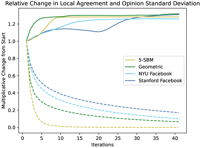
Figure 1. Number of iterations of DeGroot’s model vs. two measures of polarization in synthetic and real-world social networks.  Dotted lines plot opinion standard deviation, a variance-based measure, while solid lines plot average local agreement, a natural group-based measure, discussed in Section 5. In contrast to standard deviation, for all networks the group-based measure increases over time, which is consistent with real-world perceptions of how polarization can evolve. This finding provides evidence that the group-based measure may be a more appropriate method for quantifying polarization than the variance-based one.

Moreover, we demonstrate empirically that increases in group-based polarization are not only possible, but actually common in natural synthetic and real-world social networks. A sample result for average local agreement measure (discussed in Section 5) appears in Figure 4. Dotted lines plot opinion standard deviation, a variance-based measure of polarization. Solid lines plot average local agreement, a natural group-based measure of polarization, discussed in Section 5. In contrast to standard deviation, for all networks the group-based measure increases over time, which is consistent with real-world perceptions of how polarization evolves. We conclude that group-based measures not only have the capacity to model interesting dynamics, but also better align with perceptions of increasing polarization in reality.

For specific group-based measures, we provide additional theoretical support for increasing polarization over time. For example, in Section 4, we give a heuristic analysis for the limiting Sarle’s bimodality of opinions in stochastic block-model graphs. We show that the equilibrium value of this measure under the DeGroot dynamics is large for social network graphs with a small number of communities, a reasonable assumption of real-world networks. In Section 5, we also show that average local agreement in a social network converges to a value that depends on the second eigenvalue of the normalized adjacency matrix $\mathbf{D}^{-1}\mathbf{A}$. Polarization increases to a larger value when this eigenvalue is close to 1, which is empirically the case in a variety of real-world social network graphs.

1.2. Conclusions and Recommendations

Our findings provide formal support for using group-based measures to quantify polarization in mathematical models of opinion dynamics. The unrealistic monotonic dynamics of variance-based measures have led past studies to abandon simple opinion models like the DeGroot dynamics, and to adopt alternative, more complicated models to mathematically recover interesting polarization dynamics. For example, the Friedkin-Johnson dynamics (Friedkin and Johnsen, 1990), bounded confidence model (Lorenz, 2007), and geometric models have all seen recent attention (Ha̧zła et al., 2019; Gaitonde et al., 2021). A central conclusion of our work is that, alternatively, it may be the definition of polarization, not the model, that lacks richness for understanding societal polarization. By turning from variance-based to natural group-based polarization measures, we see interesting dynamics even in the simplest models.

Beyond our work, the recommendation to use group-based measures is also supported by empirical evidence that these measures are more aligned with how individuals perceive polarization in society than variance-based metrics (Fiorina and Abrams, 2008). In particular, it has been argued that perceived polarization does not correlate with significant absolute differences in opinion (which drive overall opinion variance) (Levendusky and Malhotra, 2015; Chambers et al., 2006). And while we cannot deny individual feelings of rising polarization in society, there is less evidence for increases in absolute difference in individual beliefs over time (Fiorina et al., 2005). It follows that the concept of “polarization” may not equate to the absolute differences in opnion measured by opinion variance. Instead, it has been argued that perceptions of polarization stem from perceptions of group-structure (Levendusky and Malhotra, 2015). In fact, even the origin of the term “polarization” in the physical sciences suggests a group-based interpretation (oed, [n.d.]). While sociological and psychological arguments for how to best quantify polarization are beyond the scope of this paper, the initial alignment between prior work and our findings is promising.

1.3. Relation to Prior Work

To the best of our knowledge, there has not been prior work on the problem of assessing the quality of various polarization metrics in mathematical models of opinion dynamics. Prior results have largely defaulted to variance-based measures. As mentioned, our work is most closely related to that of DeMarzo, Vayanos, and Zwiebel (DeMarzo et al., 2003), whose limit analysis we adopt directly (providing a new proof in Section 3). The main novelty of our work over (DeMarzo et al., 2003) is two fold. First, we show that the approach from (DeMarzo et al., 2003) has implications for a wide class of group-based polarization measures. In particular, we show that the limit result from that work implies that other group-based polarization measures converge to graph dependent values, which can be large for some graphs. Second, for different group-based measures, we provide experimental evidence and novel theoretical arguments that these group-based measures will converge to large values for natural social networks.

2. Preliminaries

Graph Notation. The DeGroot opinion dynamics model studied in this work is based on representing social connections via a weighted, undirected social graph, which we denote $G=(V,E)$. $G$ has $|V|=n$ nodes and $|E|=m$ edges, possibly including self-loops. Let $\mathbf{A}$ be the adjacency matrix of $G$, with $A_{ij}=A_{ji}>0$ if there is an edge between $i$ and $j$, and $A_{ij}=A_{ji}=0$ otherwise. Let $\mathcal{N}(i)\subseteq\{1,\ldots,n\}$ denote the set of neighbors of node $i$, which includes all $j$ for which $A_{ij}\neq 0$. If $G$ contains a self-loop at node $i$ then $A_{ii}>0$ and $i\in\mathcal{N}(i)$. Let $d_{i}=\sum_{j\in\mathcal{N}(i)}A_{ij}$ denote the degree of node $i$ and let $\mathbf{D}$ be a diagonal matrix containing $d_{1},\ldots,d_{n}$ on its diagonal.

Vector Sign Normalization. For a non-zero vector $\mathbf{x}$, let $[\mathbf{x}]^{\pm}$ denote the vector $\operatorname{sign}(x_{i})\cdot\mathbf{x}$, where $x_{i}$ is the first non-zero entry in $\mathbf{x}$. That is, $[\mathbf{x}]^{\pm}$ is equal to either $+\mathbf{x}$ or $-\mathbf{x}$, with the sign chosen to ensure that the first non-zero entry is positive.

2.1. DeGroot Opinion Dynamics

Mathematical models of opinion dynamics have been studied for decades in economics (Hegselmann and Krause, 2005; Martins, 2008; Jackson, 2008), applied math (Olfati-Saber et al., 2007; Jia et al., 2015), computer science (Urena et al., 2019; Das et al., 2014), and a variety of other fields (Goldman, 2002; Noorazar, 2020). We refer the reader to the survey in (Acemoglu and Ozdaglar, 2011). Such models typically view society as a graph, where nodes represent individuals and edges represent social connections of various strength. Connections can be in-person relationships, online relationships (e.g., edges in an online social network), or both. Simple rules and procedures then define how an individual’s opinion on an issue (represented as a single discrete or continuous value, or as a vector) evolves over time.

We focus on one of the earliest and most elegant models of opinion formation: the DeGroot opinion dynamics (French Jr., 1956; Degroot, 1974). This model is based on the idea that opinions on a topic, encoded as continuous values, propagate through the social graph via simple averaging. Nodes incorporate the beliefs of their neighbors into their own opinion over time. We formally describe the model below.

Definition 0 (DeGroot Opinion Dynamics).

Let $G=(V,E)$ be a weighted, undirected graph  with $n$ nodes, $m$ edges, adjaceny matrix $\mathbf{A}$, and degree matrix $\mathbf{D}$. For time steps $t=0,1,\ldots,T$, we associate the nodes of $G$ with an opinion vector $\mathbf{z}^{(t)}\in\operatorname*{\mathbb{R}}^{n}$ containing numerical values that represent each individual’s current view on an issue. Starting with a fixed vector of initial opinions $\mathbf{z}^{(0)}$, opinions under the DeGroot model evolve via the update:

$$z^{(t+1)}_{i}=\frac{1}{D_{ii}}\sum_{j\in\mathcal{N}(i)}A_{ij}z^{(t)}_{i},\text{or equivalently, } \mathbf{z}^{(t+1)}=\mathbf{D}^{-1}\mathbf{A}\mathbf{z}^{(t)}.$$

Convergence to Consensus. Like many other models of opinion dynamics, it is well known that the DeGroot dynamics converges to consensus in the limit. Formally, we have:

Fact 1.

If $G$ is a connected, undirected, non-bipartite graph then,

$$\mathbf{z}^{*}=\lim_{t\rightarrow\infty}\mathbf{z}^{(t)}= c\cdot\vec{\mathbf{1}} c =\sum_{i=1}^{n}\frac{d_{i}}{\sum_{j=1}^{n}d_{j}}z^{(0)}_{i}.$$ where

Note that $c$ is equal to the degree-weighted average opinion at time $0$.

As discussed, a common approach to measuring polarization on a single issue at time $t$ is to consider the overall opinion variance:

$$\operatorname{Var}[\mathbf{z}^{(t)}]=\|\mathbf{z}^{(t)}-\operatorname{mean}(\mathbf{z}^{(t)})\cdot\vec{\mathbf{1}}\|_{2}^{2}$$

Of course, if all opinions converge to the same constant value $c$, as guaranteed by Fact 1, opinion variance eventually converges to zero. While this asymptotic observation only speaks to the model’s behavior after a very long time, in the short term, variance also tends to decrease monotonically with $t$, a fact that can be proven rigorously for regular graphs (Dandekar et al., 2013a).

2.2. Group-based Polarization

In this work, we study group-based polarization metrics, which we broadly define to include any function with three properties: invariant to a shift in mean opinion, invariant to sign flips, and invariant to scaling. Formally:

Definition 0 (Group-based Polarization).

Let $f(G,\mathbf{z})$ be a function that maps an $n$-node graph $G$ and vector of opinions $\mathbf{z}\in\operatorname*{\mathbb{R}}^{n}$ to a measure of polarization. Then $f(G,\mathbf{z})$ is “group-based” if:

1. $f(G,\mathbf{z})=f(-\mathbf{z})$,

2. $f(G,\mathbf{z})=f(\mathbf{z}+c\vec{\mathbf{1}})$ for any $\mathbf{z}$ and scalar $c$, and

3. $f(G,\mathbf{z})=f(c\mathbf{z})$ for any non-zero scalar $c$.

While variance and statistical measures studied in Section 4 only depend on $\mathbf{z}$, the local measures studied in Section 5 do depend on the underlying social network which is why we include $G$ as a parameter to $f$. Variance-based measures of polarization satisfy properties (1) and (2) of Definition 2, but not (3). The last property reflects the fact that group structure should depend on relative differences in opinions instead of absolute differences. For example, an opinion vector would be considered polarized if we have two groups of individuals whose mean opinions are further apart than opinions within each group, regardless of absolute opinion difference. The resulting requirement of scale-invariance has also appeared in axiomatic treatments of clustering objectives (Kleinberg, 2003), which are closely related to group-based measures.

3. Limit Analysis

While Fact 1 implies that any variance-based measure of polarization converges to zero, this is not true for the group-based measures. Since they are both shift and scale invariant, they are insensitive to both the mean opinion (this is also true of variance-based measures) and to constant rescaling of the opinions. As such, to analyze these measures, we prove a separate convergence result for the mean-centered, normalized opinion vector, which was also observed in (DeMarzo et al., 2003). In particular, we study the vector:

$$\frac{\mathbf{z}^{(t)}-\operatorname{mean}(\mathbf{z}^{(t)})\cdot\vec{\mathbf{1}}}{\|\mathbf{z}^{(t)}-\operatorname{mean}(\mathbf{z}^{(t)})\cdot\vec{\mathbf{1}}\|_{2}}.$$

We show that, under mild conditions, in the DeGroot model this vector converges to a fixed function of the second eigenvector of the normalized social network adjacency matrix, $\mathbf{D}^{-1}\mathbf{A}$. We give a full proof below, which uses simpler arguments than (DeMarzo et al., 2003).

Theorem 1.

Let $G$ be a connected graph with adjacency and degree matrices $\mathbf{A}$ and $\mathbf{D}$. Let $\mathbf{v}_{1},\ldots,\mathbf{v}_{n}$ and $\lambda_{1},\ldots,\lambda_{n}$ be the eigenvectors and eigenvalues of $\mathbf{D}^{-1}\mathbf{A}$, in order of magnitude. I.e., $|\lambda_{1}|\geq\ldots\geq|\lambda_{n}|$ . Let $\mathbf{z}^{(0)},\ldots,\mathbf{z}^{(t)}$ be a sequence of opinion vectors updated via the DeGroot opinion dynamics as in Definition 1. Let $\mathbf{\bar{z}}^{(t)}=\mathbf{z}^{(t)}-\operatorname{mean}(\mathbf{z}^{(t)})\cdot\vec{\mathbf{1}}$ be the mean-centered opinion vector at time $t$, and let $\mathbf{\bar{v}}_{2}=\mathbf{v}_{2}-\operatorname{mean}(\mathbf{v}_{2})\cdot\vec{\mathbf{1}}$. If $|\lambda_{2}|\neq|\lambda_{3}|$ and $\langle\mathbf{D}^{1/2}\mathbf{v}_{2},z^{(0)}\rangle\neq 0$ then:

$$\bar{\mathbf{s}}^{*}\mathbin{\stackrel{{\scriptstyle\rm def}}{{=}}}\lim_{t\rightarrow\infty}\frac{[\mathbf{\bar{z}}^{(t)}]^{\pm}}{\|\mathbf{\bar{z}}^{(t)}\|_{2}}=\frac{[\mathbf{\bar{v}}_{2}]^{\pm}}{\|\mathbf{\bar{v}}_{2}\|_{2}}.$$

Recall that for a non-zero vector $\mathbf{x}$, $[x]^{\pm}$ denotes $[x]^{\pm}=\operatorname{sign}(x_{i})\cdot x$, where $x_{i}$ is the first non-zero entry in $\mathbf{x}$.

Theorem 1 holds under two mild assumptions. First, we require that $\mathbf{z}^{(0)}$ has non-zero inner product with $\mathbf{D}^{1/2}\mathbf{v}_{2}$. This holds with probability 1 whenever $\mathbf{z}^{(0)}$ involves any non-zero isotropic random component. Second, we require that $|\lambda_{2}|\neq|\lambda_{3}|$, which will hold for any natural social network, as it can be guaranteed by assuming some randomness in the edges of the network.

Under these conditions, Theorem 1 shows that the normalized opinions converge to a vector $\bar{\mathbf{s}}^{*}$ that depends on the social graph $G$ (through its second eigenvector) but does not depend on the initial opinion vector $\mathbf{z}^{(0)}$.

Proof.

From the linear algebraic form of the DeGroot update rule, we have that:

(1) $$\mathbf{z}^{(t)}=(\mathbf{D}^{-1}\mathbf{A})^{t}\mathbf{z}^{(0)}=\mathbf{D}^{-1/2}\left(\mathbf{D}^{-1/2}\mathbf{A}\mathbf{D}^{-1/2}\right)^{t}\mathbf{D}^{1/2}\mathbf{z}^{(0)}.$$

Let $\mathbf{D}^{-1/2}\mathbf{A}\mathbf{D}^{-1/2}=\mathbf{V}\mathbf{\Sigma}\mathbf{V}^{T}$ denote the eigendecomposition of the symmetric normalized adjacency matrix $\mathbf{D}^{-1/2}\mathbf{A}\mathbf{D}^{-1/2}$. $\mathbf{\Sigma}$ is a diagonal matrix that contains real-valued eigenvalues identical to those of $\mathbf{D}^{-1}\mathbf{A}$. $\mathbf{V}$ is an orthogonal matrix whose columns contain eigenvectors $\mathbf{v}_{1}^{\prime},\ldots,\mathbf{v}_{n}^{\prime}$ where $\mathbf{v}_{i}^{\prime}=\mathbf{D}^{1/2}\mathbf{v}_{i}/\|\mathbf{D}^{1/2}\mathbf{v}_{i}\|_{2}$. The eigenvalues of the normalized adjacency matrix of an undirected graph always lie in $[-1,1]$ and, since $\mathbf{A}$ is connected, there is exactly one eigenvector with eigenvalue $\lambda_{1}=1$. It can be verified that the corresponding eigenvector of $\mathbf{D}^{-1/2}\mathbf{A}\mathbf{D}^{-1/2}$ is equal to $\mathbf{v}_{1}^{\prime}=\mathbf{D}^{1/2}\vec{\mathbf{1}}/\|\mathbf{D}^{1/2}\vec{\mathbf{1}}\|_{2}$.

We expand (1), using that $(\mathbf{D}^{-1/2}\mathbf{A}\mathbf{D}^{-1/2})^{t}=\mathbf{V}\mathbf{\Sigma}^{t}\mathbf{V}^{T}$ since $\mathbf{V}$ is orthogonal. For $i=1,\ldots,n$, let $c_{i}=\langle\mathbf{v}_{i},\mathbf{D}^{1/2}\mathbf{z}^{(0)}\rangle$. We have that:

$$\mathbf{z}^{(t)}=\mathbf{D}^{-1/2}\cdot\left(c_{1}\lambda_{1}^{t}\mathbf{v}_{1}+c_{2}\lambda_{2}^{t}\mathbf{v}_{2}+...+c_{n}\lambda_{n}^{t}\mathbf{v}_{n}\right),$$

and thus $\mathbf{\bar{z}}^{(t)}=\mathbf{{z}^{(t)}}-\operatorname{mean}\left(\mathbf{{z}}^{(t)}\right)$ equals:

$$\mathbf{\bar{z}}^{(t)} =c_{1}\lambda_{1}^{t}\mathbf{D}^{-1/2}\mathbf{v}_{1}^{\prime}-\operatorname{mean}\left(c_{1}\lambda_{1}^{t}\mathbf{D}^{-1/2}\mathbf{v}_{1}^{\prime}\right)\cdot\vec{\mathbf{1}}$$

$$+c_{2}\lambda_{2}^{t}\mathbf{D}^{-1/2}\mathbf{v}_{2}^{\prime}-\operatorname{mean}\left(c_{2}\lambda_{2}^{t}\mathbf{D}^{-1/2}\mathbf{v}_{2}^{\prime}\right)\cdot\vec{\mathbf{1}}$$

$$\hskip 72.00008pt\vdots$$

$$+c_{n}\lambda_{n}^{t}\mathbf{D}^{-1/2}\mathbf{v}_{n}^{\prime}-\operatorname{mean}\left(c_{n}\lambda_{n}^{t}\mathbf{D}^{-1/2}\mathbf{v}_{n}^{\prime}\right)\cdot\vec{\mathbf{1}}.$$

Note that $\mathbf{D}^{-1/2}\mathbf{v}_{1}^{\prime}$ is a scaling of the all ones vectors, so the first term in the sum above is zero. Letting $\mathbf{\bar{v}}_{i}=\mathbf{D}^{-1/2}\mathbf{v}_{i}^{\prime}-\operatorname{mean}(\mathbf{D}^{-1/2}\mathbf{v}_{i}^{\prime})\cdot\vec{\mathbf{1}}$, we are left with:

$$\frac{\mathbf{\bar{z}}^{(t)}}{\|\mathbf{\bar{z}}^{(t)}\|_{2}}=\frac{c_{2}\lambda_{2}^{t}\mathbf{\bar{v}}_{2}+c_{3}\lambda_{3}^{t}\mathbf{\bar{v}}_{3}+\ldots+c_{n}\lambda_{n}^{t}\mathbf{\bar{v}}_{n}}{\|c_{2}\lambda_{2}^{t}\mathbf{\bar{v}}_{2}+c_{3}\lambda_{3}^{t}\mathbf{\bar{v}}_{3}+\ldots+c_{n}\lambda_{n}^{t}\mathbf{\bar{v}}_{n}\|_{2}}.$$

We first note that $\|\mathbf{\bar{v}}_{i}\|_{2}>0$ for all $i=2,\ldots,n$. To see why this is the case, observe that to have $\|\mathbf{\bar{v}}_{i}\|_{2}=0$, it must be that $\mathbf{v}_{i}^{\prime}=c\mathbf{D}^{1/2}\vec{\mathbf{1}}$ for some constant $c$. However, this cannot be the case because $\mathbf{v}_{i}^{\prime}$ is orthogonal to $\mathbf{v}_{1}^{\prime}=c\mathbf{D}^{1/2}\vec{\mathbf{1}}$. Combined with our assumption that $c_{2}=\langle\mathbf{D}^{1/2}\mathbf{v}_{2},z^{(0)}\rangle\neq 0$, it follows that $\|c_{2}\mathbf{\bar{v}}_{2}\|_{2}\geq 0$. Then, by our assumption that $|\lambda_{2}|\neq|\lambda_{3}$, we have $|\lambda_{2}|>|\lambda_{i}|$ for all $i=3,\ldots,n$. So, for any $\epsilon>0$, there is some $t$ such that $\|c_{3}\lambda_{3}^{t}\mathbf{\bar{v}}_{3}+\ldots+c_{n}\lambda_{n}^{t}\mathbf{\bar{v}}_{n}\|_{2}\leq\epsilon\|c_{2}\mathbf{\bar{v}}_{2}\|_{2}$. We conclude that:

$$\lim_{t\rightarrow\infty}\frac{[\mathbf{\bar{z}}^{(t)}]^{\pm}}{\|\mathbf{\bar{z}}^{(t)}\|_{2}} =\lim_{t\rightarrow\infty}\frac{[c_{2}\lambda_{2}^{t}\mathbf{\bar{v}}_{2}+\ldots+c_{n}\lambda_{n}^{t}\mathbf{\bar{v}}_{n}]^{\pm}}{\|c_{2}\lambda_{2}^{t}\mathbf{\bar{v}}_{2}+\ldots+c_{n}\lambda_{n}^{t}\mathbf{\bar{v}}_{n}\|_{2}}=\frac{[c_{2}\lambda_{2}^{t}\mathbf{\bar{v}}_{2}]^{\pm}}{\|c_{2}\lambda_{2}^{t}\mathbf{\bar{v}}_{2}\|_{2}}.$$

This proves the theorem since $\frac{[c_{2}\lambda_{2}^{t}\mathbf{\bar{v}}_{2}]^{\pm}}{\|c_{2}\lambda_{2}^{t}\mathbf{\bar{v}}_{2}\|_{2}}=\frac{[\mathbf{\bar{v}}_{2}]^{\pm}}{\|\mathbf{\bar{v}}_{2}\|_{2}}$ for any $c_{2},\lambda_{2}$. ∎

3.1. Implications for Ideological Alignment

In the work of DeMarzo, Vayanos, and Zwiebel (DeMarzo et al., 2003), Theorem 1 is used to explain a phenomenon involving multiple opinion vectors, each defined for a different issue. They call the phenomenon “unidimensional opinions”, but we prefer the terminology ideological alignment. Ideological alignment occurs when large groups of individuals simultaneously differ in opinion on many issues (Evans, 2003; Abramowitz and Saunders, 2008). Also refereed to as “party sorting” (Fiorina and Abrams, 2008), this phenomenon is well-documented in the real-world, and there is strong survey-based evidence that it has increased in recent years (Levendusky, 2009; Pew Research Center, 2014). Since it accentuates differences between groups, ideological alignment has likely contributed to increased perception of polarization (Abramowitz and Saunders, 2008).

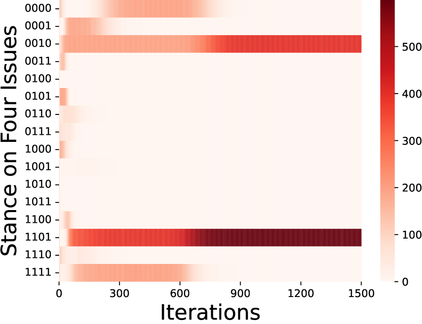
(a) 5-SBM

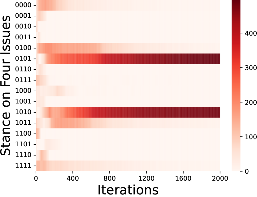
(b) Random Geometric

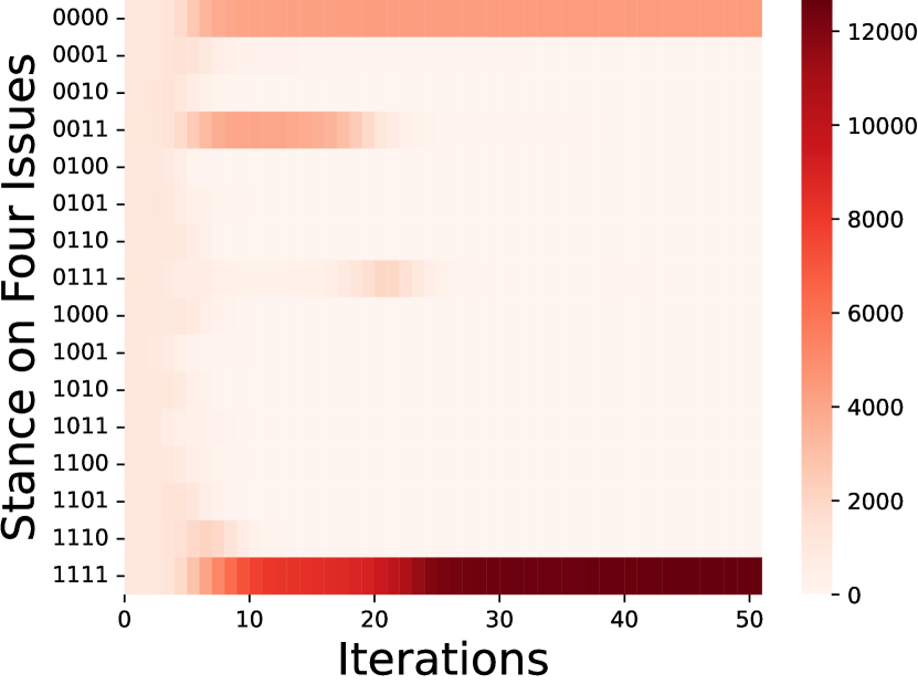
(c) NYU Facebook

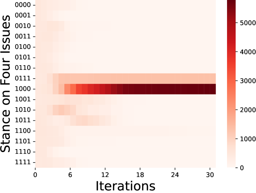
(d) Stanford Facebook

Figure 2. Heat map of “binary opinion profiles” across $m=4$ different issues by iteration of the DeGroot model. Each row corresponds to one of $2^{m}$ difference opinion profiles, and the color at time $t$ indicates the number of nodes whose current opinions match that profile. As predicted by Corollary 2, all individuals eventually sort into just two profiles, leading to perfect ideological alignment.

Theorem 1 provides striking mathematical support for the emergence of ideological alignment. In particular, an an immediate corollary of the result is that, in the limit, individuals will perfectly sort into exactly two groups that simultaneously disagree on all issues –i.e., for each issue, the members of one group will all have opinions on the opposite side of the mean as the other group. We formalize their observation from (DeMarzo et al., 2003) in Corollary 2.

Corollary 2.

Consider a social graph $G$ and $m$ different initial opinion vectors $z_{1}^{(0)},\cdots,z_{m}^{(0)}$ satisfying the assumptions of Theorem 1. Apply the DeGroot opinion dynamics to each vector for $t$ steps to obtain opinions $\mathbf{z}_{1}^{(t)},\cdots,\mathbf{z}_{m}^{(t)}$, and let $\mathbf{s}_{i}^{(t)}=\operatorname{sign}(\mathbf{z}_{i}^{(t)}-\operatorname{mean}(\mathbf{z}_{i}^{(t)})\cdot\vec{\mathbf{1}})$. Consider the matrix $\mathbf{S}^{(t)}=[\mathbf{s}_{1}^{(t)},\ldots,\mathbf{s}_{m}^{(t)}]$. In the limit as $t\rightarrow\infty$, $\mathbf{S}^{(t)}$ will only contain two unique rows.

Each row of $\mathbf{S}^{(t)}$ corresponds to a single node (individual) in $G$. It contains $\{+1,-1\}$ entries indicating if that individual has opinion below or above the mean for each of the $m$ topics at time $t$. The row can thus be viewed an individual’s “binary opinion profile”. The takeaway from Corollary 2 is that, while there are $2^{m}$ possible opinion profiles, for large enough $t$ just two will dominate, becoming adopted by every individual. We visualized this alignment for four social networks in Figure 2. Opinions were initialized randomly, so the rows of $\mathbf{S}^{(0)}$ are distributed evenly between all $2^{m}$ possible binary opinion profiles. However, as $t$ increases, we eventually see convergence to a state where $\mathbf{S}^{(t)}$ has just two unique binary rows. The number of iterations until convergence varies by network.

While an interesting phenomenon, one potential limitation of ideological alignment as a polarization measure is that, like variance-based measures, it converges to the same extreme state for all social networks – albeit to a state that is fully polarized instead of a fully in consensus. In contrast, the other group-based measures of polarization discussed in this paper converge to network dependent quantities, so their dynamics over time will natural differ within different social structure and can be impacted by outside influences that effect that structure, like social media or propaganda.

3.2. Implications for Group-Based Polarization

The foundation of our work is the insight that Theorem 1 actually has implications on the limiting behavior of any group-based measure of polarization. Formally:

Corollary 3.

Let $f(G,\mathbf{z})$ be a group-based polarization metric according to Definition 2 that is continuous with respect to the argument $\mathbf{z}\in\operatorname*{\mathbb{R}}^{n}$. If the conditions of Theorem 1 hold, then

$$\lim_{t\rightarrow\infty}f(G,\mathbf{z}^{(t)})=f(G,\mathbf{v}_{2})$$

where $z^{(t)}$ and $\mathbf{v}_{2}$ are as defined as in Theorem 1.

Corollary 3 implies that, unlike variance-based measures which always converge to zero, under the mild assumptions of Theorem 1, any group-based measure of polarization converges to a value that depends on the social graph $G$. At the same time, the value does not depend on the starting opinions $\mathbf{z}^{(0)}$. With Corollary 3 in place, we analyze several different group-based measures of polarization in the subsequent sections.

4. Statistical Measures

We start with statistical measures that, like variance, consider only the numerical values in an opinion vector $\mathbf{z}$, without taking into account the ordering of entries or their structure with respect to $G$. For example, the following common statistical measure of bimodality incorporates $3^{\text{rd}}$ and $4^{\text{th}}$ moment information from $\mathbf{z}$:

Definition 0 (Sarle’s Bimodality Coefficient).

Consider an opinion vector $\mathbf{z}$ and let $\mathbf{\bar{z}}$ denote $\mathbf{\bar{z}}=\mathbf{z}-\operatorname{mean}(\mathbf{z})$. Then the bimodality $\beta(\mathbf{z})$ is written in terms of the skewness $\gamma$ and kurtosis $\kappa$ as follows:

$$\beta(\mathbf{z})=\frac{\gamma^{2}+1}{\kappa}\textrm{ where }\gamma=\frac{\operatorname{mean}(\mathbf{\bar{z}}^{3})}{\operatorname{mean}(\mathbf{\bar{z}}^{2})^{3/2}}\textrm{ and }\kappa=\frac{\operatorname{mean}(\mathbf{\bar{z}}^{4})}{\operatorname{mean}(\mathbf{\bar{z}}^{2})^{2}}.$$

The bimodality coefficient of Definition 1 has been used as a measure of opinion polarization, e.g. in (DiMaggio et al., 1996), where it was compared against variance-based measures. The measure lies between $0$ and $1$, with $1$ indicating maximum polarization. However, even a random isotropic vector $\mathbf{r}$ (e.g., a vector with i.i.d. random Gaussian entries) will have bimodality $\beta(\mathbf{r})\approx 1/3$, since the skewness of a normal random variable is 0 and the kurtosis is 3. Accordingly, we consider a vector of opinions “polarized” if the bimodality is larger than $1/3$.

Figure 3. Opinion bimodality $\beta(\mathbf{z})$ plotted by iteration of DeGroot’s opinion dynamics model run on the same 5 block SBM graph, and initialized with five randomly generated starting opinion vectors. As predicted by Corollary 3, in all cases opinion bimodality converges to a fixed non-zero equilibrium bimodality that depends on the graph.

We demonstrate Corollary 3 in Figure 3. We generate a Stochastic Block Model (SBM) network (Holland et al., 1983; Abbe, 2017) on $n=1000$ nodes with five communities (blocks). The probability of an edge within a block is $p=1/10$ and the probability of an edge between blocks is $q=1/100$. We then initialize five random starting opinion vectors, each with i.i.d. standard normal entries. We plot the bimodality of opinions as they evolve via the DeGroot dynamics. By 1000 iterations, there is clear convergence to the bimodality of the second eigenvector of the SBM, which, at $.658$, is much larger than the bimodalities of the starting opinions around $1/3$. So, while bimodality evolves in a highly non-monotonic way, it ultimately increases over time.

$1^{\text{st}}$ Quartile	Median	$3^{\text{rd}}$ Quartile
.805	.917	.952

Table 1. Statistics of equilibrium bimodality for 100 college social networks from the Facebook100 data set (Traud et al., 2012).

Increases in bimodality are even more pronounced in real-world social networks. We ran a similar experiment for 100 college social networks from the Facebook100 data set (Traud et al., 2012) and observed that for all but five networks, bimodality increases under the DeGroot dynamics with random starting opinions. The median and quartiles of the equilibrium bimodality (computed directly from the second eigenvector of each network) are included in Table 1. We conclude that the simple bimodality coefficient offers a clear contrast with variance-based measures of polarization that decrease over time.

An informal analysis of SBM graphs offers theoretical support for increases in bimodality in natural social networks with a small number of well connected communities. Specifically, we argue that any SBM with a small number of blocks typically has equilibrium bimodality greater than $1/3$. We thus expect increasing bimodality under the DeGroot model if opinions are randomly initialized.

Observation 1.

For a $k$-block SBM graph, the equilibrium bimodality is approximated by the sample bimodality of a normal random variable when $k$ samples are taken, which has expected value greater than $1/3$ for small $k$.

We sketch a proof of Observation 1: While the bimodality of the normal distribution is $1/3$, the empirical bimodality computed from a finite number of samples tends to over-estimate the true bimodality. While it is difficult to obtain an exact expression for the expectation of the sample bimodality, the sample kurtosis has expectation $3\frac{k-1}{k+1}$ (Joanes and Gill, 1998). Sample kurtosis is thus an underestimate for small $k$, explaining the overestimate of bimodality, which depends on the inverse kurtosis. Now consider the expected symmetric normalized adjacency matrix $\mathbf{\bar{D}}^{-1/2}\mathbf{\bar{A}}\mathbf{\bar{D}}^{-1/2}$ of an SBM graph, where $\mathbf{\bar{D}}=\operatorname*{\mathbb{E}}[\mathbf{D}]$ and $\mathbf{\bar{A}}=\operatorname*{\mathbb{E}}[\mathbf{A}]$. It is not hard to see that the top $k$ eigenvectors of $\mathbf{\bar{D}}^{-1/2}\mathbf{\bar{A}}\mathbf{\bar{D}}^{-1/2}$ can be spanned by $\vec{\mathbf{1}}$ as well as $k$ block indicator vectors, each which is $1$ for the nodes in a single community, and $0$ for all other nodes. Since the actually normalized adjacency matrix $\mathbf{{D}}^{-1/2}\mathbf{{A}}\mathbf{{D}}^{-1/2}$ can be viewed as a perturbed version of $\mathbf{\bar{D}}^{-1/2}\mathbf{\bar{A}}\mathbf{\bar{D}}^{-1/2}$, we roughly expect its first $k$ eigenvectors to also be spanned by $\vec{\mathbf{1}}$ and the $k$ block vectors – a formal statement could be made by appealing to the Davis-Kahan perturbation theorem (Davis and Kahan, 1970). Moreover, the $2^{\text{nd}}$ through the $(k-1)^{\text{st}}$ eigenvalues of $\mathbf{\bar{D}}^{-1/2}\mathbf{\bar{A}}\mathbf{\bar{D}}^{-1/2}$ are all the same, so we roughly expect the second eigenvector of $\mathbf{{D}}^{-1/2}\mathbf{{A}}\mathbf{{D}}^{-1/2}$ to be a random linear combination of the $k$ block indicator vector, plus some scaling of $\vec{\mathbf{1}}$ (which has no impact on bimodality). If the random linear combination is isotropic, the second eigenvector will look exactly like $k$ samples from a random Gaussian distribution, each repeated $n/k$ times. This vector the same bimodality as $k$ random Gaussian samples.

Observation 1 is visualized in Figure 4, which was generated by computing the equilibrium opinion bimodality for 100 random $k$-SBM graphs with $1000$ and $2000$ nodes. While it approaches $1/3$ as $k$ increases, equilibrium bimodality is much larger for small $k$. We also plot the sample bimodality of $k$ i.i.d Gaussian samples (also computed using 100 trials), which as predicted by Observation 1, correlates well with the observed bimodality of the $k$-SBM.

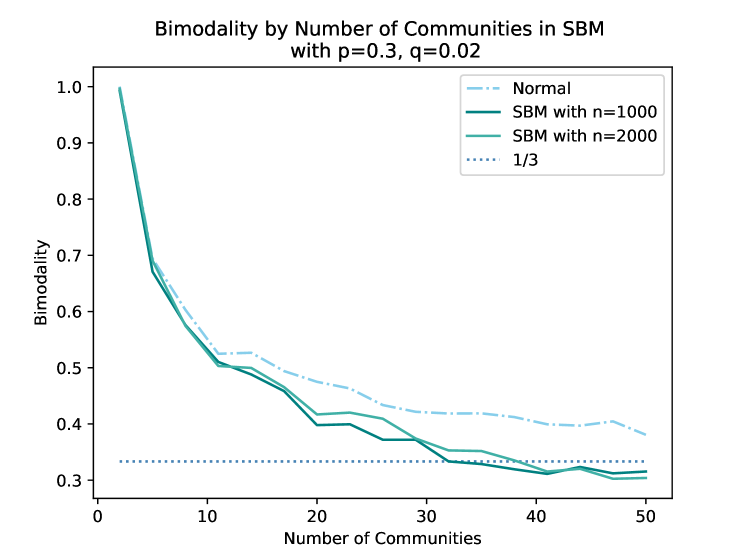
Figure 4. Average equilibrium bimodality of $k$-SBM graphs with intra-block edge probability $3/10$ and inter-block edge probability $2/100$. Bimodality converges to the bimodality of a random normal variable for large $k$, which is $1/3$, but as predicted in Observation 1, can be much larger for small $k$.

5. Local Measures

Another interesting class of group-based polarization measures are those that take into account local structure of the social graph $G$. Such measures are motivated by the fact that individuals are most heavily exposed to the opinions of their social connections – i.e., their neighborhood in $G$. Individuals likely also have a sense of the overall mean opinion in $G$ (e.g., from the news), but do not simultaneously sense all opinions in a social network.

In this section we introduce and study one such measure, which we call average local agreement that takes these considerations into account. In particular, we define the local agreement of a vertex $i$ to be the ratio of $i$’s neighbors whose opinion falls on the same side (above or below) the mean opinion $\operatorname{mean}(\mathbf{z})$ as $i$. We posit that high local agreement correlates with high perceptions of polarization, as individuals who feel more isolated in a group, away from those differing opinion, tends to experience feelings of polarization (Levendusky and Malhotra, 2015).

We formally define average local agreement below. We use $\operatorname{sign}(\mathbf{x})$ to denote the operation that rounds every entry of a vector $\mathbf{x}$ to +1 or -1, taking the convention that if $x_{i}=0$, $[\operatorname{sign}(\mathbf{x})]_{i}=+1$.

Definition 0 (Average Local Agreement).

Let $G$ be a social network on $n$ nodes and let $\mathbf{z}\in\operatorname*{\mathbb{R}}^{n}$ be an opinion vector. Let $\mathbf{s}=\operatorname{sign}(\mathbf{z}-\operatorname{mean}(\mathbf{z})\cdot\vec{\mathbf{1}})$. The average local agreement $\mathcal{L}(G,\mathbf{z})$ equals:

$$\mathcal{L}(G,\mathbf{z}) =\frac{1}{n}\sum_{i=1}^{n}\frac{1}{d_{i}}\sum_{j\in\mathcal{N}(i)}\mathbbm{1}[s_{i}=s_{j}]$$

$$\text{where \,\,}\mathbf{s}=\operatorname{sign}(\mathbf{z}-\operatorname{mean}(\mathbf{z})\cdot\vec{\mathbf{1}}).$$

Recall that $\mathcal{N}(i)$ denotes the neighborhood of node $i$ in $G$, and $\mathbbm{1}[\cdot]$ is an indicator function that evaluates to $1$ if the expression in brackets is true, and to $0$ otherwise.

Like bimodality, average local agreement is a group-based measure as specified in Definition 2. So, as in Corollary 3, we have that in the DeGroot dynamics, under the assumptions of Theorem 1, $\lim_{t\rightarrow\infty}\mathcal{L}(G,\mathbf{z}^{(t)})=\mathcal{L}(G,\mathbf{v}_{2})$, where $z^{(t)}$ and $\mathbf{v}_{2}$ are as defined as in the theorem. Average local agreement is bounded between $[0,1]$ and we expect a value of $1/2$ for randomly initialized opinions. So, any value above $1/2$ is considered “polarized”. As shown in Table 2, we observe very high average local agreement in the limit for real-world social networks. For all but two of the 100 networks in the Facebook100 data set, this measure of polarization converged to a value above $.6$, and was typically well above $.9$. In Figure 5 we also visualize local agreement over time for a random 5-SBM graph and a random geometric graph, as well as the Swarthmore Facebook graph (chosen for its small size). In all cases, “bubbles” of high local agreement visibly emerge, with average local agreement increasing to $.785$, $.954$, and $.941$ for the three graphs, respectively.

$1^{\text{st}}$ Quartile	Median	$3^{\text{rd}}$ Quartile
.904	.947	.960

Table 2. Statistics of the equilibrium average local agreement, $\mathcal{L}(G,\mathbf{v}_{2})$ for the Facebook100 data set (Traud et al., 2012).

	0 Iterations	5 Iterations	Equilibrium	Equilibrium Opinions
5 Block SBM
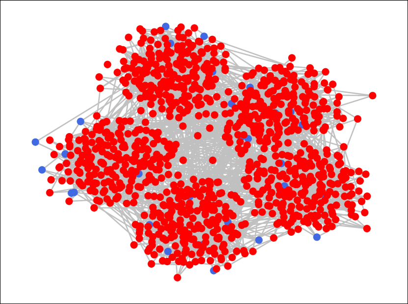
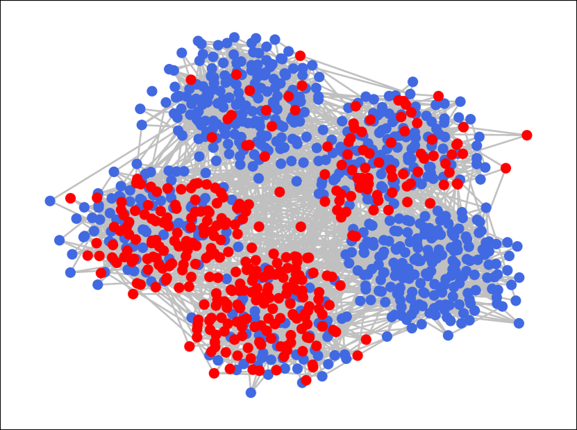
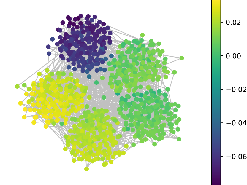
Random Geometric
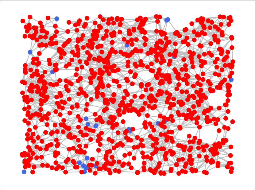
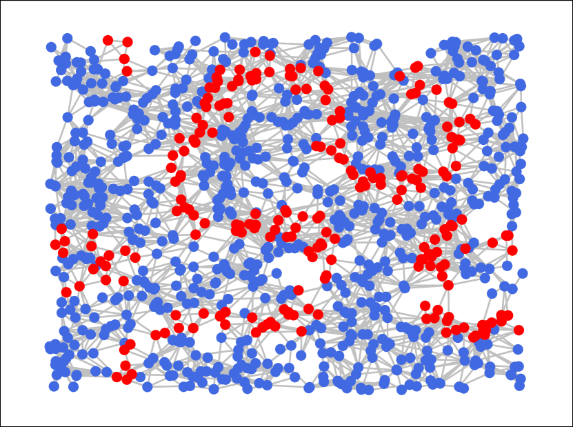
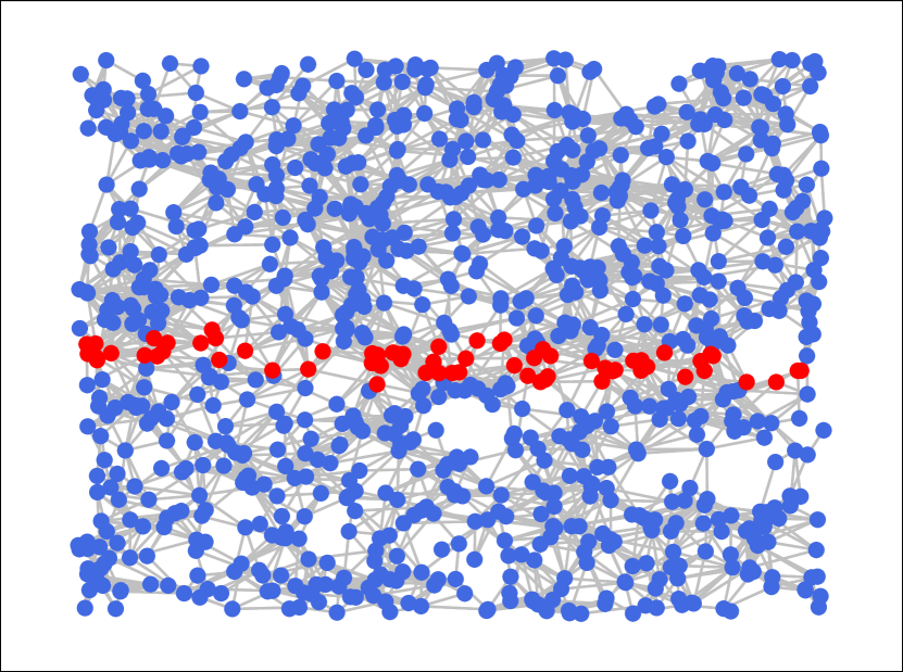
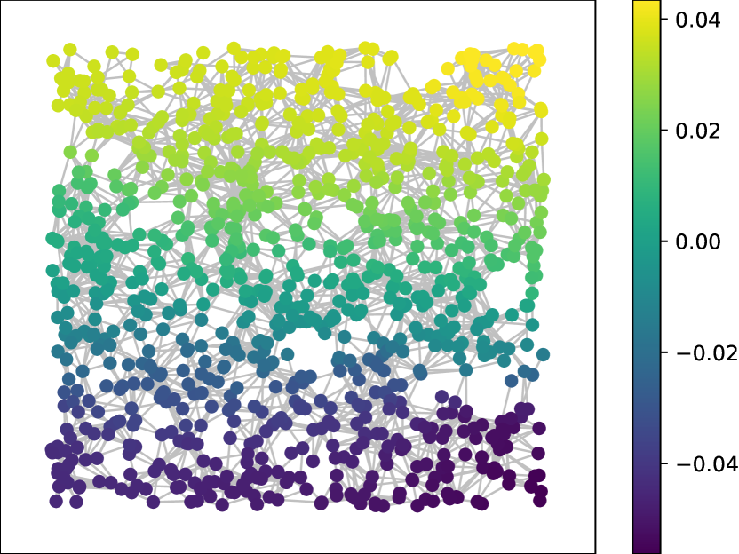
Swarthmore Facebook

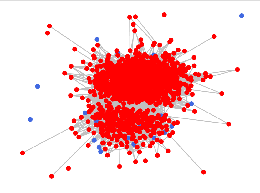
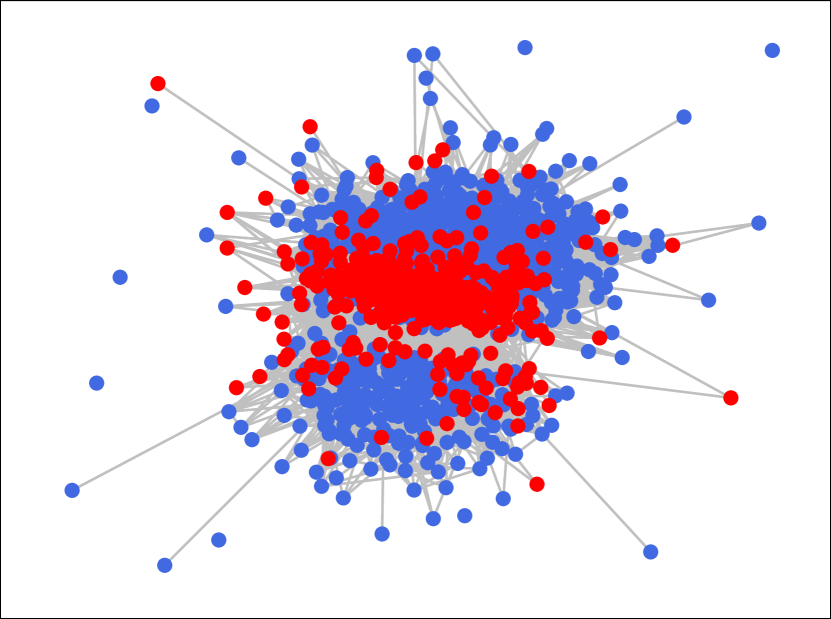
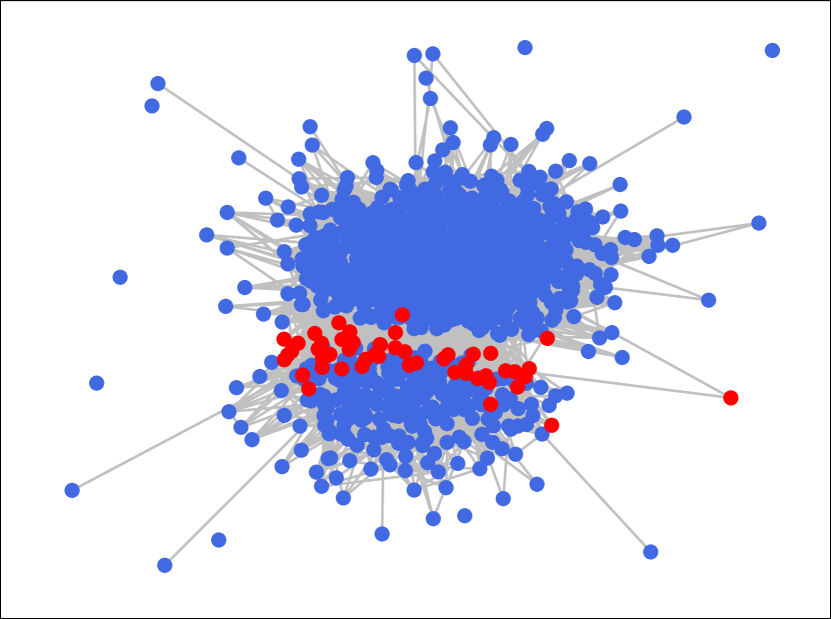
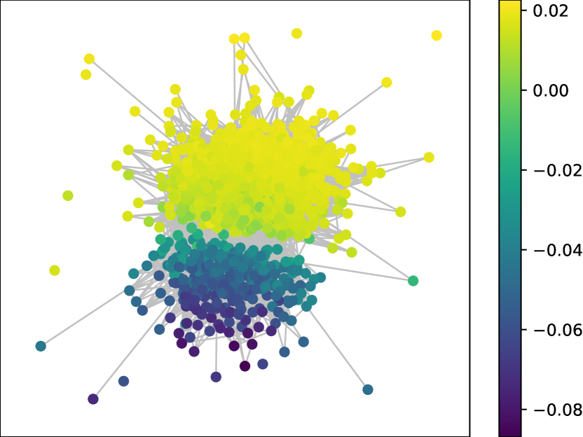
Figure 5. A visualization of local agreement by number of DeGroot iterations for three social networks. Nodes are colored blue for individuals with at least 2/3 of their neighbors on the same side of the mean opinion, and red otherwise. The last column shows the normalized differences from the mean opinion at equilibrium ($\bar{\mathbf{s}}^{*}$ from Theorem 1). In all cases, strong clusters of high local agreement emerge, which may lead to increased perceptions of opinion polarization.

To better understand the steep increase in this group-based polarization metric theoretically, we show that for an unweighted, regular graph $G$, average local agreement has a simple linear algebraic form. Ultimately, the following claim will help us relate the measure to spectral properties of the underlying social graph $G$.

Claim 1.

Let $G$ be an unweighted $d$-regular graph with no self-loops. Let $\mathbf{z}$ be a vector of opinions and let $\mathbf{s}=\operatorname{sign}(\mathbf{z}-\operatorname{mean}(\mathbf{z})\cdot\vec{\mathbf{1}})$. Then, the average local agreement $\mathcal{L}(G,\mathbf{z})$ equals:

$$\mathcal{L}(G,\mathbf{z}) =\frac{\mathbf{s}^{T}\mathbf{A}\mathbf{s}}{2nd}+\frac{1}{2} \text{where \,\,}\mathbf{s} =\operatorname{sign}(\mathbf{z}-\operatorname{mean}(\mathbf{z})\cdot\vec{\mathbf{1}}).$$

Proof.

For a node $i$, let $p_{i}=\sum_{j\in\mathcal{N}(i)}\mathbbm{1}[s_{j}=+1]$ denote the number of nodes in $\mathcal{N}(i)$ that are on the positive side of the mean and let $q_{i}=\sum_{j\in\mathcal{N}(i)}\mathbbm{1}[s_{j}=-1]$ denote the number of nodes on the negative side of the mean. Let $a_{i}$ denote the number of nodes in $\mathcal{N}(i)$ that agree with node $i$ (i.e., are on the same side of the mean) and let $b_{i}$ denote the number of nodes that disagree. We can write:

$$a_{i} =\begin{cases}p_{i}&\text{ if }s_{i}=+1\\ q_{i}&\text{ if }s_{i}=-1\\ \end{cases} b_{i}=\begin{cases}p_{i}&\text{ if }s_{i}=-1\\ q_{i}&\text{ if }s_{i}=+1\\ \end{cases}$$

Observe that the $i^{\text{th}}$ entry of $\mathbf{A}\mathbf{s}$ equals $p_{i}-q_{i}$, and thus:

$$\mathbf{s}^{T}\mathbf{A}\mathbf{s}=\sum_{i=1}^{n}s_{i}(p_{i}-q_{i})=\sum_{i=1}^{n}a_{i}-b_{i}.$$

Next note that $a_{i}+b_{i}=d$ and thus $nd=\sum_{i=1}^{n}a_{i}+b_{i}$. So we have $\mathbf{s}^{T}\mathbf{A}\mathbf{s}+nd=\sum_{i=1}^{n}2a_{i}$. Dividing by $2nd$ gives the result because $\mathcal{L}(G,\mathbf{z})=\frac{1}{n}\sum_{i=1}^{n}\frac{a_{i}}{d}$. ∎

With Claim 1 in place, we make the following observation:

Observation 2.

For an unweighted graph $G$, we can approximate the equilibrium average local agreement $\lim_{t\rightarrow\infty}\mathcal{L}(G,\mathbf{z}^{(t)})$ by

$$\lim_{t\rightarrow\infty}\mathcal{L}(G,\mathbf{z}^{(t)})\approx\frac{\lambda_{2}}{2}+\frac{1}{2},$$

where $\lambda_{2}$ is the second eigenvalue of $G$’s normalized adjacency matrix.

According to this claim, we expect to see high equilibrium local agreement – i.e., increasing polarization – in any graph with a second eigenvalue close to $1$, which includes any graph with strong community, and thus most natural social networks. For example, the Facebook100 networks had an average second eigenvalue of $.871$. Observation 2 predicts that this would lead to a mean equilibrium average local agreement of approximately $.936$, which is extremely close to the observed mean of $.948$.

To establish Observation 2, again assume that $G$ is $d$-regular with no self-loops. Note that for a regular graph, the second eigenvalue of $\mathbf{D}^{-1}\mathbf{A}$ is equal to that of $\mathbf{D}^{-1/2}\mathbf{A}\mathbf{D}^{-1/2}$. By Corollary 3, we have that $\lim_{t\rightarrow\infty}\mathcal{L}(G,\mathbf{z}^{(t)})=\mathcal{L}(G,\mathbf{v}_{2})$. And by Claim 1:

$$\mathcal{L}(G,\mathbf{v}_{2}) =\frac{\operatorname{sign}(\mathbf{v}_{2}^{T})\mathbf{A}\operatorname{sign}(\mathbf{v}_{2})}{2nd}+\frac{1}{2}$$

$$=\frac{\operatorname{sign}(\mathbf{v}_{2}^{T})\mathbf{D}^{-1/2}\mathbf{A}\mathbf{D}^{-1/2}\operatorname{sign}(\mathbf{v}_{2})}{2n}+\frac{1}{2}$$

Observation 2 then immediately follows by noticing that

$$\operatorname{sign}(\mathbf{v}_{2}^{T})\mathbf{D}^{-1/2}\mathbf{A}\mathbf{D}^{-1/2}\operatorname{sign}(\mathbf{v}_{2})\approx n\mathbf{v}_{2}^{T}\mathbf{D}^{-1/2}\mathbf{A}\mathbf{D}^{-1/2}\mathbf{v}_{2}=n\lambda_{2}.$$

The approximation is exact if all entries in the unit vector $\mathbf{v}_{2}$ have magnitude $1/\sqrt{n}$. It tends to hold a close approximation in other networks, which can be formalized via well-known connections between balanced cut problems and the second eigenvector (McSherry, 2001; Spielman, 2019).

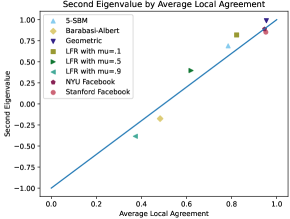
Figure 6. Average local agreement at equilibrium plotted against the second normalized adjacency matrix eigenvalue for several random graphs generated with the NetworkX package (Hagberg et al., 2008), and for the NYU and Stanford Facebook graphs. The values closely align with the linear relationship predicted by Observation 2 (plotted as a solid line).

In Figure 6, we empirically confirm the relationship described in Observation 2 by examining a variety of random graphs with widely varying second eigenvalue. We find that the correlation between average local agreement and second eigenvalue in the Facebook100 data set is statistically significant ($p=5e^{-5}$) with a Pearson correlation of $r=.392$.

Finally, we comment on the rate at which average local agreement converges to its equilibrium value. Since this rate depends on how quickly the normalized difference vector converges to $\bar{s}^{*}$ under the DeGroot model, we expect it to scale linearly with the inverse of the second eigenvalue gap, $\frac{|\lambda_{2}|-|\lambda_{3}|}{|\lambda_{2}|}$. We confirm this relationship on the Facebook100 data set, where we see a statistically significant ($p=7e^{-6}$) correlation between inverse second eigengap and average number of iterations until convergence to the final average local agreement when starting with a random opinion vector. The Pearson correlation coefficient of the relationship is $r=.451$.

In contrast, the rate at which the opinion vector converges to $\mathbf{z}^{*}$ depends inversely on the first eigengap $\frac{|\lambda_{1}|-|\lambda_{2}|}{|\lambda_{1}|}$. As such, when the second eigengap is large compared to the first, we expect local agreement to increase more quickly than opinion variance decreases, which might contribute to perceptions of growing polarization.

6. Conclusion

In this work we established that natural group-based polarization measures display interesting dynamics under the standard DeGroot opinion formation model. Unlike heavily studied variance-based measures, we showed both empirically and theoretically that group-based measures can increase over time, and often do increase quite significantly in natural social networks.

We leave a number of questions for future research. As discussed, recent work on mathematical models of opinion dynamics has sought to understand the impact of outside actors (who can modify the graph $G$ is some way) on individual opinions and polarization (Gaitonde et al., 2021; Abebe et al., 2021). There is little work on how such modifications impact group-based polarization, and if they can accelerate its emergence.

Another challenging question it to determine the “right” group-based measure of polarization for use in opinion dynamics studies. Our work establishes that group-based measures in general are more in line with real-world polarization than variance-based measures, but more in-depth studies of e.g. political opinion surveys would be needed to determine exactly which group-based measures best align with perceived polarization. Currently, there is some experimental evidence for the value of ideological alignment as a meaningful polarization metric (Levendusky, 2009; Fiorina et al., 2005), but statistical measures of bimodality and “local” metrics have received less attention.

References

- (1)
- oed ([n.d.]) [n.d.]. “polarization, n.”. In Oxford English Dictionary. Oxford University Press. https://www.oed.com/view/Entry/146757.
- Abbe (2017) Emmanuel Abbe. 2017. Community detection and stochastic block models: recent developments. The Journal of Machine Learning Research 18, 1 (2017), 6446–6531.
- Abebe et al. (2021) Rediet Abebe, T.-H. Chan, Jon Kleinberg, Zhibin Liang, David Parkes, Mauro Sozio, and Charalampos E. Tsourakakis. 2021. Opinion Dynamics Optimization by Varying Susceptibility to Persuasion via Non-Convex Local Search. ACM Trans. Knowl. Discov. Data 16, 2 (2021).
- Abramowitz and Saunders (2008) Alan I. Abramowitz and Kyle L. Saunders. 2008. Is Polarization a Myth? The Journal of Politics 70, 2 (2008), 542–555.
- Acemoglu and Ozdaglar (2011) Daron Acemoglu and Asuman Ozdaglar. 2011. Opinion Dynamics and Learning in Social Networks. Dynamic Games and Applications 1, 1 (2011), 3–49.
- Bianco and Smyth (2020) W. Bianco and R. Smyth. 2020. The Bicameral Roots of Congressional Deadlock: Analyzing Divided Government Through the Lens of Majority Rule. Social Science Quarterly 101 (2020), 1712–1727.
- Binder (2014) Sarah Binder. 2014. Polarized we govern? https://www.brookings.edu/research/polarized-we-govern/
- Brooks and Porter (2020) Heather Z Brooks and Mason A Porter. 2020. A model for the influence of media on the ideology of content in online social networks. Physical Review Research 2, 2 (2020).
- Carothers and O’Donohue (2019) Thomas Carothers and Andrew O’Donohue (Eds.). 2019. Democracies Divided: The Global Challenge of Political Polarization. Brookings Institution Press.
- Chambers et al. (2006) John R. Chambers, Robert S. Baron, and Mary L. Inman. 2006. Misperceptions in Intergroup Conflict: Disagreeing About What We Disagree About. Psychological Science 17, 1 (2006), 38–45.
- Chitra and Musco (2020) Uthsav Chitra and Christopher Musco. 2020. Analyzing the Impact of Filter Bubbles on Social Network Polarization. In Proceedings of the 13th International Conference on Web Search and Data Mining. 115–123.
- Dandekar et al. (2013a) Pranav Dandekar, Ashish Goel, and David Lee. 2013a. Biased Assimilation, Homophily and the Dynamics of Polarization. Proceedings of the National Academy of Sciences of the United States of America 110 (03 2013). https://doi.org/10.1073/pnas.1217220110
- Dandekar et al. (2013b) Pranav Dandekar, Ashish Goel, and David T Lee. 2013b. Biased assimilation, homophily, and the dynamics of polarization. Proceedings of the National Academy of Sciences 110, 15 (2013), 5791–5796.
- Das et al. (2014) Abhimanyu Das, Sreenivas Gollapudi, and Kamesh Munagala. 2014. Modeling opinion dynamics in social networks. In Proceedings of the \nth7 International Conference on Web Search and Data Mining (WSDM). ACM, 403–412.
- Davis and Kahan (1970) C. Davis and W. Kahan. 1970. The Rotation of Eigenvectors by a Perturbation. III. SIAM J. Numer. Anal. 7, 1 (1970), 1–46.
- Degroot (1974) Morris H. Degroot. 1974. Reaching a Consensus. J. Amer. Statist. Assoc. 69, 345 (1974), 118–121.
- DeMarzo et al. (2003) Peter M. DeMarzo, Dimitri Vayanos, and Jeffrey Zwiebel. 2003. Persuasion Bias, Social Influence, and Unidimensional Opinions. The Quarterly Journal of Economics 118, 3 (2003), 909–968.
- Difranzo and Gloria-Garcia (2017) Dominic Difranzo and Kristine Gloria-Garcia. 2017. Filter bubbles and fake news. XRDS: Crossroads, The ACM Magazine for Students 23 (04 2017), 32–35. https://doi.org/10.1145/3055153
- DiMaggio et al. (1996) Paul DiMaggio, John Evans, and Bethany Bryson. 1996. Have American’s Social Attitudes Become More Polarized? Amer. J. Sociology 102, 3 (1996), 690–755.
- Evans (2003) John H. Evans. 2003. Have Americans’ Attitudes Become More Polarized?—An Update. Social Science Quarterly 84, 1 (2003), 71–90.
- Fiorina and Abrams (2008) Morris P. Fiorina and Samuel J. Abrams. 2008. Political Polarization in the American Public. Annual Review of Political Science 11, 1 (2008), 563–588.
- Fiorina et al. (2005) Morris P. Fiorina, Samuel J. Abrams, and Jeremy C. Pope. 2005. Culture war: The myth of a polarized America. Pearson-Longman.
- French Jr. (1956) John R. P. French Jr. 1956. A formal theory of social power. Psychological Review 63, 3 (1956), 181–194.
- Friedkin and Johnsen (1990) Noah E. Friedkin and Eugene C. Johnsen. 1990. Social influence and opinions. The Journal of Mathematical Sociology 15, 3-4 (1990), 193–206.
- Gaitonde et al. (2020) Jason Gaitonde, Jon Kleinberg, and Eva Tardos. 2020. Adversarial perturbations of opinion dynamics in networks. In Proceedings of the \nth21 ACM Conference on Economics and Computation (EC). 471–472.
- Gaitonde et al. (2021) Jason Gaitonde, Jon Kleinberg, and Éva Tardos. 2021. Polarization in Geometric Opinion Dynamics. Proceedings of the \nth22 ACM Conference on Economics and Computation (EC) (2021).
- Geschke et al. (2019) Daniel Geschke, Jan Lorenz, and Peter Holtz. 2019. The triple-filter bubble: Using agent-based modelling to test a meta-theoretical framework for the emergence of filter bubbles and echo chambers. British Journal of Social Psychology 58, 1 (2019), 129–149.
- Goldman (2002) Alvin Goldman. 2002. Knowledge in a social world. Philosophy and Phenomenological Research 64, 1 (2002).
- Green et al. (2020) Jon Green, Jared Edgerton, Daniel Naftel, Kelsey Shoub, and Skyler J. Cranmer. 2020. Elusive consensus: Polarization in elite communication on the COVID-19 pandemic. Science Advances 6, 28 (2020).
- Hagberg et al. (2008) Aric A. Hagberg, Daniel A. Schult, and Pieter J. Swart. 2008. Exploring Network Structure, Dynamics, and Function using NetworkX. In Proceedings of the 7th Python in Science Conference. 11 – 15.
- Hart et al. (2020) P. Sol Hart, Sedona Chinn, and Stuart Soroka. 2020. Politicization and Polarization in COVID-19 News Coverage. Science Communication 42, 5 (2020), 679–697.
- Ha̧zła et al. (2019) Jan Ha̧zła, Yan Jin, Elchanan Mossel, and Govind Ramnarayan. 2019. A Geometric Model of Opinion Polarization. arXiv:910.05274 (2019).
- Hegselmann and Krause (2002) Rainer Hegselmann and Ulrich Krause. 2002. Opinion dynamics and bounded confidence: Models, analysis and simulation. Journal of Artificial Societies and Social Simulation 5 (2002), 1–24.
- Hegselmann and Krause (2005) Rainer Hegselmann and Ulrich Krause. 2005. Opinion dynamics driven by various ways of averaging. Computational Economics 25, 4 (2005), 381–405.
- Holland et al. (1983) Paul W. Holland, Kathryn Blackmond Laskey, and Samuel Leinhardt. 1983. Stochastic blockmodels: First steps. Social Networks 5, 2 (1983), 109–137.
- Holone (2016) Harald Holone. 2016. The filter bubble and its effect on online personal health information. Croatian medical journal 57, 3 (2016), 298.
- Jackson (2008) Matthew O Jackson. 2008. Social and economic networks. Princeton University Press.
- Jia et al. (2015) Peng Jia, Anahita MirTabatabaei, Noah E Friedkin, and Francesco Bullo. 2015. Opinion dynamics and the evolution of social power in influence networks. SIAM review 57, 3 (2015), 367–397.
- Joanes and Gill (1998) D. N. Joanes and C. A. Gill. 1998. Comparing Measures of Sample Skewness and Kurtosis. Journal of the Royal Statistical Society. Series D (The Statistician) 47, 1 (1998), 183–189.
- Jones (2015) David R. Jones. 2015. Declining Trust in Congress: Effects of Polarization and Consequences for Democracy. The Forum 13, 3 (2015), 375–394. https://doi.org/doi:10.1515/for-2015-0027
- Kleinberg (2003) Jon Kleinberg. 2003. An Impossibility Theorem for Clustering. In Advances in Neural Information Processing Systems 16 (NeurIPS), Vol. 15.
- Layman et al. (2006) Geoffrey C. Layman, Thomas M. Carsey, and Juliana Menasce Horowitz. 2006. Party Polartization in American Politics: Characteristics, Causes, and Consequences. Annual Review of Political Science 9, 1 (2006), 83–110.
- Levendusky (2009) Matthew Levendusky. 2009. The partisan sort. University of Chicago Press.
- Levendusky and Malhotra (2015) Matthew S. Levendusky and Neil Malhotra. 2015. (Mis)perceptions of Partisan Polarization in the American Public. Public Opinion Quarterly 80, S1 (10 2015), 378–391.
- Lorenz (2007) Jan Lorenz. 2007. Continuous Opinion Dynamics Under Bounded Confidence: A Survey. International Journal of Modern Physics C 18, 12 (2007), 1819–1838.
- Martins (2008) André CR Martins. 2008. Continuous opinions and discrete actions in opinion dynamics problems. International Journal of Modern Physics C 19, 04 (2008).
- McCoy and Somer (2019) Jennifer McCoy and Murat Somer. 2019. Toward a Theory of Pernicious Polarization and How It Harms Democracies: Comparative Evidence and Possible Remedies. The ANNALS of the American Academy of Political and Social Science 681 (01 2019), 234–271.
- McCright and Dunlap (2011) Aaron M McCright and Riley E Dunlap. 2011. The politicization of climate change and polarization in the American public’s views of global warming, 2001–2010. The Sociological Quarterly 52, 2 (2011), 155–194.
- McSherry (2001) Frank McSherry. 2001. Spectral Partitioning of Random Graphs. In Proceedings of the \nth42 Annual IEEE Symposium on Foundations of Computer Science (FOCS).
- Monmouth University Polling Institute (2019) Monmouth University Polling Institute. 2019. Americans Feel Divided On Core Values.
- Musco et al. (2018) Cameron Musco, Christopher Musco, and Charalampos E. Tsourakakis. 2018. Minimizing Polarization and Disagreement in Social Networks. In Proceedings of the \nth27 International World Wide Web Conference (WWW). 369–378.
- Noorazar (2020) Hossein Noorazar. 2020. Recent advances in opinion propagation dynamics: a 2020 survey. The European Physical Journal Plus 135, 6 (2020), 1–20.
- Olfati-Saber et al. (2007) Reza Olfati-Saber, J Alex Fax, and Richard M Murray. 2007. Consensus and cooperation in networked multi-agent systems. Proc. IEEE 95, 1 (2007), 215–233.
- Pariser (2011) Eli Pariser. 2011. The filter bubble: what the internet is hiding from you. Penguin UK.
- Pew Research Center (2014) Pew Research Center. 2014. Political Polarization in the American Public. (2014).
- Saveski et al. (2022) Martin Saveski, Nabeel Gillani, Ann Yuan, Prashanth Vijayaraghavan, and Deb Roy. 2022. Perspective-taking to Reduce Affective Polarization on Social Media. In ICWSM’22: International AAAI Conference on Web and Social Media.
- Spielman (2019) Daniel A. Spielman. 2019. Spectral and Algebraic Graph Theory. Yale University. httphttp://cs-www.cs.yale.edu/homes/spielman/sagt/.
- Traud et al. (2012) Amanda L Traud, Peter J Mucha, and Mason A Porter. 2012. Social structure of Facebook networks. Physica A: Statistical Mechanics and its Applications 391, 16 (2012), 4165–4180.
- Urena et al. (2019) Raquel Urena, Gang Kou, Yucheng Dong, Francisco Chiclana, and Enrique Herrera-Viedma. 2019. A review on trust propagation and opinion dynamics in social networks and group decision making frameworks. Information Sciences 478 (2019), 461–475.