Abstract

This work develops a class of probabilistic algorithms for the numerical solution of nonlinear, time-dependent partial differential equations (PDEs). Current state-of-the-art PDE solvers treat the space- and time-dimensions separately, serially, and with black-box algorithms, which obscures the interactions between spatial and temporal approximation errors and misguides the quantification of the overall error. To fix this issue, we introduce a probabilistic version of a technique called method of lines. The proposed algorithm begins with a Gaussian process interpretation of finite difference methods, which then interacts naturally with filtering-based probabilistic ordinary differential equation (ODE) solvers because they share a common language: Bayesian inference. Joint quantification of space- and time-uncertainty becomes possible without losing the performance benefits of well-tuned ODE solvers. Thereby, we extend the toolbox of probabilistic programs for differential equation simulation to PDEs.

1 INTRODUCTION

This work develops a class of probabilistic numerical (PN) algorithms for the solution of initial value problems based on partial differential equations (PDEs). PDEs are a widely-used way of modelling physical interdependencies between temporal and spatial variables. With the recent advent of physics-informed neural networks (Raissi et al.,, 2019), neural operators (Lu et al.,, 2021; Li et al.,, 2021), and neural ordinary/partial differential equations (Chen et al.,, 2018; Gelbrecht et al.,, 2021), PDEs have rapidly gained popularity in the machine learning community, too. Let $F$, $h$, and $g$ be given nonlinear functions. Let the domain $\Omega\subset\mathbb{R}^{d}$ with boundary $\partial\Omega$ be sufficiently well-behaved so that the PDE (below) has a unique solution. $\mathcal{D}$ shall be a differential operator. The reader may think of the Laplacian, $\mathcal{D}=\sum_{i=1}^{d}\frac{\partial^{2}}{\partial x_{i}^{2}}$, but the algorithm is not restricted to this case. The goal is to approximate an unknown function $u:\Omega\rightarrow\mathbb{R}^{L}$ that solves

$$\frac{\partial}{\partial t}u(t,x) =F(t,x,u(t,x),\mathcal{D}u(t,x)),$$ (1)

for $t\in[t_{0},t_{\text{max}}]$ and $x\in\Omega$, subject to initial condition

$$u(t_{0},x) =h(x),\quad x\in\Omega,$$ (2)

and boundary conditions $\mathcal{B}u(t,x)=g(x)$, $x\in\partial\Omega$. The differential operator $\mathcal{B}$ is usually the identity (Dirichlet conditions) or the derivative along normal coordinates (Neumann conditions). Except for only a few problems, PDEs do not admit closed-form solutions, and numerical approximations become necessary. This also affects machine learning strategies such as physics-informed neural networks or neural operators, for example, because they rely on fast generation of training data.

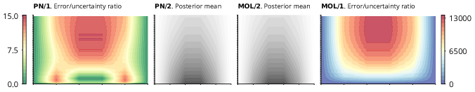
Figure 1: PNMOL fixes bad calibration of the MOL/ODE filter combination: Posterior means and error/uncertainty ratios of PNMOL (left) and MOL with a conventional PN solver (right) on a fine time grid ($y$-axis) and a coarse space grid ($x$-axis) for the heat equation. The means are indistinguishable (*/2). PN w/ MOL is poorly calibrated (error/uncertainty ratios $\sim 10^{5}$; */1), but PNMOL acknowledges all inaccuracies.

One common strategy for solving PDEs, called the method of lines (MOL; Schiesser,, 2012), first discretises the spatial domain $\Omega$ with a grid ${\mathbb{X}}:=(x_{0},...,x_{N})$, and then uses this grid to approximate the differential operator $\mathcal{D}$ with a matrix-vector product

$$(\mathcal{D}u)(t,{\mathbb{X}})\approx Du(t,{\mathbb{X}}),\quad D\in\mathbb{R}^{(N+1)\times(N+1)},$$ (3)

where we use the notation $u(t,{\mathbb{X}})=(u(t,x_{n}))_{n=0}^{N}$. Replacing the differential operator $\mathcal{D}$ with the matrix $D$ turns the PDE into a system of ordinary differential equations (ODEs; more information about $D$ follows). Standard ODE solvers can then numerically solve the resulting initial value problem.

This approach has one central problem. Discretising the spatial domain, and only then applying an ODE solver, turns the PDE solver into a pipeline of two numerical algorithms instead of a single algorithm. This is bad because as a result of this serialisation, the error estimates returned by the ODE solver are unreliable. The solver lacks crucial information about whether the spatial grid consists of, say, $N=4$ or $N=10^{7}$ points. It is intuitive that a coarse spatial grid puts a lower bound on the overall precision, even if the ODE solver uses small time steps. But since this is not “known” to the ODE solver, not even to a probabilistic one, it may waste computational resources by needlessly decreasing its step-size and may deliver (severely) overconfident uncertainty estimates (for example, Fig. 1). This phenomenon will be confirmed by the experiments in Section 7. Such overconfident uncertainty estimates are essentially useless to a practitioner, which complicates the usage of method of lines approaches within probabilistic simulation of differential equations; for example, in the context of latent force inference or inverse problems.

The present work provides a solution to this problem by revealing a way of tracking spatiotemporal correlations in the PDE solutions while preserving the computational advantages of traditional MOL through a probabilistic numerical solver. The main idea of the present paper is the following. The error that is introduced by approximating the differential operator $\mathcal{D}$ with a matrix $D$ can be quantified probabilistically, and its time-evolution acts as a latent force on the resulting ODE. The combined posterior over the PDE solution and the latent force can be computed efficiently with a PN ODE solver. More specifically, we contribute:

Probabilistic discretisation

Sections 2 and 3 present a probabilistic technique for constructing finite-dimensional approximations of $\mathcal{D}$ that quantify the discretisation error. It translates an unsymmetric collocation method (Kansa,, 1990) to the language of Gaussian processes and admits efficient, sparse approximations akin to radial-basis-function-generated finite-difference formulas (Tolstykh and Shirobokov,, 2003).

Calibrated PDE filter

Building on the probabilistic discretisation, Section 4 explains how the discretisation and the ODE solver need not be treated as two separate entities. By applying the idea behind the method of lines to a global Gaussian process prior, it becomes evident how the discretisation uncertainty naturally evolves over time. With a filtering-based probabilistic ODE solver (“ODE filter”), posteriors over the latent error process and the PDE solution can be inferred in linear time, and without ignoring spatial uncertainties like traditional MOL algorithms do.

Section 5 explains hyperparameter choices and calibration. Section 6 discusses connections to existing work. Section 7 demonstrates the advantages of the approach over conventional MOL. Altogether, PNMOL enriches the toolbox of probabilistic simulations of differential equations by a calibrated and efficient PDE solver.

2 PN DISCRETISATION

This section derives how to approximate a differential operator $\mathcal{D}$ by a matrix $D$. Let $u_{x}(z)\sim\operatorname{\mathcal{GP}}(0,\gamma^{2}k_{x})$ be a Gaussian process on $\Omega$ with covariance kernel $k_{x}(z,z^{\prime})$ and output scale $\gamma>0$. The presentation in Section 4 will assume a Gaussian process prior $u(t,x)\sim\operatorname{\mathcal{GP}}(0,\gamma^{2}k_{t}\otimes k_{x})$, thus the notation “$u_{x}$” motivates $u_{x}$ as “the $x$-part of $u(t,x)$”. The boundary operator $\mathcal{B}$ is ignored in the remainder because it can be treated in the same way as $\mathcal{D}$. Complete formulas including $\mathcal{B}$, are in Supplement A.

The objective is to approximate the PDE dynamics in a way that circumvents the differential operator $\mathcal{D}$,

$$f(t,{\mathbb{X}},u_{x}({\mathbb{X}}))\approx F(t,{\mathbb{X}},u_{x}({\mathbb{X}}),(\mathcal{D}u_{x})({\mathbb{X}})),$$ (4)

that is, $\mathcal{D}u_{x}$ disappears from Eq. 1 because $f$ replaces $F$. For linear differential operators $\mathcal{D}$, this reduces to replacing $(\mathcal{D}u_{x})({\mathbb{X}})$ with a matrix-vector product $Du_{x}({\mathbb{X}})$, $D\in\mathbb{R}^{(N+1)\times(N+1)}$ (recall Eq. 3), for example, by using the method proposed below. $\mathcal{D}$ must not be present in the discretised model, because otherwise, the PDE does not translate into a system of ODEs, and we cannot proceed with the method of lines. But with an approximate derivative based on only matrix-vector arithmetic, the computational efficiency of ODE solvers can be exploited to infer an approximate PDE solution.

Since $u$ is a Gaussian process, applying the linear operator $\mathcal{D}$ yields another Gaussian process $\mathcal{D}u_{x}\sim\operatorname{\mathcal{GP}}(0,\mathcal{D}^{2}k_{x})$, where we abbreviate $\mathcal{D}^{2}k_{x}(z,z^{\prime})=\mathcal{D}\mathcal{D}^{*}k_{x}(z,z^{\prime})$ and $\mathcal{D}^{*}$ is the adjoint of $\mathcal{D}$ (in the present context, this means applying $\mathcal{D}$ to $z^{\prime}$ instead of $z$). Conditioning $u_{x}$ on realisations of $u_{x}({\mathbb{X}})$, and then applying $\mathcal{D}$, yields another Gaussian process with moments

$$\hat{m}(z) =W_{\mathbb{X}}(z)u_{x}({\mathbb{X}}),$$ (5a)

$$\hat{k}(z,z^{\prime}) =(\mathcal{D}^{2}k_{x})(z,z^{\prime})-W_{\mathbb{X}}(z)k_{x}({\mathbb{X}},{\mathbb{X}})W_{\mathbb{X}}(z^{\prime})^{\top},$$ (5b)

$$W_{\mathbb{X}}(z) :=(\mathcal{D}k_{x})(z,{\mathbb{X}})k_{x}({\mathbb{X}},{\mathbb{X}})^{-1}.$$ (5c)

Let $\xi_{x}\sim\operatorname{\mathcal{GP}}(0,\gamma^{2}\hat{k})$. $\xi_{x}$ is independent of $u_{x}$, since $\hat{k}$ only depends on $\mathcal{D}$, $k_{x}$, and ${\mathbb{X}}$, not on $u_{x}({\mathbb{X}})$. Then,

$$W_{\mathbb{X}}(z)u_{x}({\mathbb{X}})+\xi_{x}(z)\sim\operatorname{\mathcal{GP}}(0,\mathcal{D}\mathcal{D}^{*}k_{x})$$ (6)

follows, which implies

$$p(\mathcal{D}u_{x}(\cdot))=p(W_{\mathbb{X}}(\cdot)u_{x}({\mathbb{X}})+\xi(\cdot)).$$ (7)

In particular, when evaluated on the grid, we obtain the matrix-vector formulation of the differential operator

$$(\mathcal{D}u_{x})({\mathbb{X}})=W_{\mathbb{X}}({\mathbb{X}})u_{x}({\mathbb{X}})+\xi_{x}({\mathbb{X}}).$$ (8)

Eq. 8 yields $\mathcal{D}u_{x}$ solely as a transformation of values of $u_{x}$ with known, additive Gaussian noise $\xi_{x}$. Altogether, the above derivation identifies the differentiation matrix $D$ and the error covariance $E$

$$D:=W_{\mathbb{X}}({\mathbb{X}}),\quad E:=\hat{k}({\mathbb{X}},{\mathbb{X}}).$$ (9)

If we know $u_{x}({\mathbb{X}})$, we have an approximation to $(\mathcal{D}u_{x})({\mathbb{X}})$ that is wrong with covariance $\gamma^{2}E$. The matrix $E$ makes the approach probabilistic (and new).

There are two possible interpretations for $D$ (and $E$). $D$ appears in a method for solving PDEs $\mathcal{D}u_{x}=f$ with radial basis functions, called unsymmetric collocation, or Kansa’s method (Kansa,, 1990; Hon and Schaback,, 2001; Schaback,, 2007). A related method, called symmetric collocation (Fasshauer,, 1997, 1999), has been built on and translated into a Bayesian probabilistic numerical method by Cockayne et al., (2017). The following derivation shows that a translation is possible for the probabilistic discretisation, respectively unsymmetric collocation, as well: Eq. 7 explains

$$(\mathcal{D}u_{x})({\mathbb{X}})\mid u_{x}({\mathbb{X}}),\xi_{x} \sim\delta\left[Du_{x}({\mathbb{X}})+\xi_{x}\right]$$ (10a)

$$=\mathcal{N}(Du_{x}({\mathbb{X}}),\gamma^{2}E).$$ (10b)

$\delta$ is the Dirac delta. In other words, $D$ and $E$ (respectively $D$ and $\xi$) estimate $\mathcal{D}u_{x}$ from values of $u_{x}$ at a set of grid-points – just like finite difference formulas do. By construction, it is a Bayesian probabilistic numerical algorithm in the technical sense of Cockayne et al., (2019). Supplement B contains a formal proof of this statement.

The limitations of the above probabilistic discretisation are twofold. First, computation of the differentiation matrix $D$ involves inverting the kernel Gram matrix $k_{x}({\mathbb{X}},{\mathbb{X}})$. For large point sets, this matrix is notoriously ill-conditioned (Schaback,, 1995). Second, computation – and application – of $D$ is expensive because $D$ is a dense matrix with as many rows and columns as there are points in ${\mathbb{X}}$. Since loosely speaking, a derivative is a “local” phenomenon (other than e.g. computing integrals), intuition suggests that $\mathcal{D}u_{x}$ can be approximated more cheaply by exploiting this locality. This thought leads to localised differentiation matrices and probabilistic numerical finite differences.

3 PN FINITE DIFFERENCES

The central idea of an efficient approximation of the probabilistic discretisation is to approximate the derivative of $u_{x}$ at each point $x_{n}$ in ${\mathbb{X}}$ individually. This leads to a row-by-row assembly of $D$, which can be sparsified naturally and without losing the ability to quantify numerical discretisation/differentiation uncertainty.

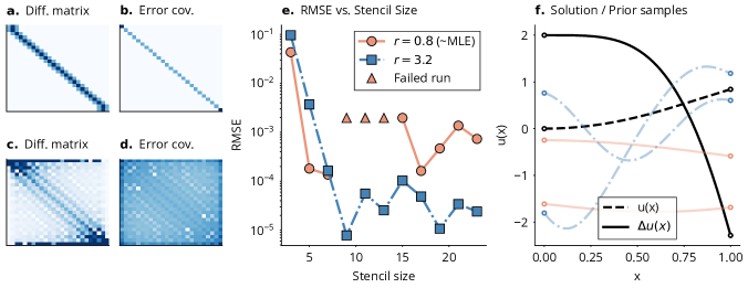
Figure 2: Discretise the Laplacian with a local and global approximation: The target is the Laplacian $\mathcal{D}=\Delta$ of $u(x)=\sin(\|x\|^{2})$ (f). Left: Sparsity pattern of the differentiation matrix and error covariance matrix for the localised approximation (a, b) and the global approximation (c, d) on a mesh with $N=25$ points. The approximation is least certain at the boundaries. Centre: The root-mean-square error between $\Delta u$ and its approximation decreases with an increased stencil size but the approximation breaks down for larger stencils (e), likely due to ill-conditioned kernel Gram matrices. A maximum likelihood estimate of the input scale $r\in\mathbb{R}$ of the square exponential kernel $k(x,y)=e^{-r^{2}\|x-y\|^{2}}$ based on data $u_{x}(x)$ alone does not necessarily lead to well-conditioned system matrices, nor does it generally imply a low RMSE (e). Right: Samples from the prior GP $u_{x}$ for both length scales are shown next to the solution and the target function (f; the colours match the colours in the RMSE plot). Increasing stencil sizes improves the accuracy until stability concerns arise.

Write the matrix $D$ as a vertical stack of $N+1$ row-vectors, $D=(d_{0},...,d_{N})^{\top}$, and denote by $e_{n}$ the $n$th diagonal element of $E$, i.e. the variance of the approximation of $\mathcal{D}u_{x}$ at the $n$th grid-point in ${\mathbb{X}}$. Thus,

$$\mathcal{D}u_{x}(x_{n})\mid u_{x}({\mathbb{X}}),\xi_{x}\sim\delta[d_{n}^{\top}u_{x}({\mathbb{X}})+\xi_{x,n}]$$ (11)

with the scalar random variable $\xi_{x,n}\sim\mathcal{N}(0,\gamma^{2}e_{n})$. If, in Eq. 11, we replace $u_{x}({\mathbb{X}})$ by the values of $u_{x}$ at only a local neighbourhood of $x_{n}$ (a “stencil”),

$$x_{\operatorname{loc}(n)}=\{x_{n-k},...,x_{n},...,x_{n+k}\},$$ (12)

the general form of Eq. 11 is preserved, but $d_{n}$ consists of only $2k+1$ elements, with $k\ll N$,

$$d_{n}=(\mathcal{D}k_{x})(x_{n},{x}_{\operatorname{loc}(n)})k_{x}(x_{\operatorname{loc}(n)},x_{\operatorname{loc}(n)})^{-1}$$ (13)

instead of $N+1$ elements. The error $e_{n}$ becomes

$$e_{n} :=(\mathcal{D}^{2}k_{x})(x_{n},x_{n})-d_{n}k_{x}(x_{\operatorname{loc}(n)},x_{\operatorname{loc}(n)})d_{n}^{\top}.$$ (14)

If the coefficients in the new $d_{n}$ are all embedded into $D$ according to the indices of $x_{\operatorname{loc}(n)}$ in ${\mathbb{X}}$, $D$ becomes sparse and $E$ becomes diagonal. More precisely, $D_{ij}\neq 0$ if and only if $j\in\operatorname{loc}(i)$. On a one-dimensional domain $\Omega$, and with $k=1$, $D$ is a banded matrix with bandwidth 3. Furthermore, due to the point-by-point construction, choosing $k=N/2$ implies that the original $D$ from Section 2 is recovered; however, $E$ remains diagonal. The sparse approximation resolves many of the performance issues that persist with the global approximation (Fig. 2).

The sparsified differentiation matrix is known as the radial-basis-function-generated finite difference matrix (Driscoll and Fornberg,, 2002; Shu et al.,, 2003; Tolstykh and Shirobokov,, 2003; Fornberg and Flyer,, 2015). The correspondence to finite-difference formulas stems from the fact that if $k_{x}$ were a polynomial kernel and the mesh ${\mathbb{X}}$ were equidistant and one-dimensional, the coefficients in $D$ would equal the standard finite difference coefficients (Fornberg,, 1988). The advantage of the more general, kernel-based finite difference approximation over polynomial coefficients is a more robust approximation, especially for non-uniform grid points and in higher dimensions (Tolstykh and Shirobokov,, 2003; Fornberg and Flyer,, 2015). The Bayesian point of view does not only add uncertainty quantification in the form of $E$ but also reveals that a practitioner may choose suitable kernels $k_{x}$ to include prior information into the PDE simulation.

4 PN METHOD OF LINES

The previous two sections have been concerned with approximating the derivative of a function, purely from observations of this function on a grid. Next, we use these strategies to solve time-dependent PDEs. To this end, we combine the probabilistic discretisation with an ODE filter. As opposed to non-probabilistic MOL, this combination quantifies the leak of information between the space discretisation and the ODE solution. Simply put, what is commonly treated as a pipeline of disjoint solvers, becomes more of a single algorithm.

4.1 Spatiotemporal Prior Process

For any function $\varphi=\varphi(t)$, let $\vec{\varphi}$ be the stack of $\varphi$ and its first $\nu$ derivatives, $\vec{\varphi}(t):=(\varphi(t),\dot{\varphi}(t),...,\varphi^{(\nu)}(t))$. This abbreviation is convenient because some stochastic processes (like the integrated Wiener or Matérn process) do not have the Markov property, but the stack of state and derivatives does. The following assumption is integral for the probabilistic method of lines.

Assumption 1.

Assume a Gaussian process prior with separable covariance structure,

$$u=u(t,x)\sim\operatorname{\mathcal{GP}}(0,\gamma^{2}k_{t}\otimes k_{x})$$ (15)

for some output-scale $\gamma>0$. $k_{t}\otimes k_{x}$ is the product kernel $(k_{t}\otimes k_{x})(t,t^{\prime},x,x^{\prime})=k_{t}(t,t^{\prime})k_{x}(x,x^{\prime})$.

Compared to the traditional method of lines, where the temporal and spatial dimensions are treated independently and with black-box methods, Assumption 1 is mild: even though the covariance is separable, the algorithm still starts with a single, global Gaussian process. Assumption 1 allows choosing temporal kernels that eventually lead to a fast algorithm:

Assumption 2.

Assume $k_{t}$ is a covariance kernel that allows conversion to a linear, time-invariant stochastic differential equation (SDE) in the following sense: For any $\upsilon\sim\operatorname{\mathcal{GP}}(0,\gamma^{2}k_{t})$, $\vec{\upsilon}$ solves the SDE

$$\,\textup{d}\vec{\upsilon}(t)=A\vec{\upsilon}(t)\,\textup{d}t+B\,\textup{d}w(t)$$ (16)

subject to Gaussian initial conditions

$$\vec{\upsilon}(t_{0})\sim\mathcal{N}(m_{0},\gamma^{2}C_{0}),$$ (17)

for $A$, $B$, $m_{0}$, and $C_{0}$ that derive from $k_{t}$, and for a one-dimensional Wiener process $w$ with diffusion $\gamma^{2}$.

Assumption 2 is satisfied, for instance, for the integrated Wiener process or the Matérn process; many more examples are given in Chapter 12 of the book by Särkkä and Solin, (2019). Assumptions 1 and 2 unlock the machinery of probabilistic ODE solvers.

Next, we add spatial correlations into the prior SDE model. The following Lemma 3 will simplify the derivations further below (Solin,, 2016).

Lemma 3.

Let $k_{t}$ be a covariance function that satisfies Assumption 2. Let $M\in\mathbb{R}^{q\times q}$ be a matrix. For a process $\varphi\sim\operatorname{\mathcal{GP}}(0,\gamma^{2}k_{t}\otimes M)$, $\vec{\varphi}$ solves

$$\,\textup{d}\vec{\varphi}(t)=(A\otimes I)\vec{\varphi}(t)\,\textup{d}t+(B\otimes I)\,\textup{d}\hat{w}(t),$$ (18)

subject to Gaussian initial conditions

$$\vec{\varphi}(t_{0})\sim\mathcal{N}(m_{0}\otimes\mathbf{1},\gamma^{2}C_{0}\otimes M),$$ (19)

where $\hat{w}$ is a $q$-dimensional Wiener process with constant diffusion $\gamma^{2}M$, and $I\in\mathbb{R}^{q\times q}$ is the identity. $m_{0}\otimes\mathbf{1}$ is a vertical stack of $d$ copies of $m_{0}$.

Lemma 3 suggests that a spatiotemporal prior (Assumption 1) may be restricted to a spatial grid without losing the computational benefits that SDE priors provide. Abbreviate $U(t):=u(t,{\mathbb{X}})$. Lemma 3 gives rise to an SDE representation for $U(t)$ by choosing $M=k_{x}({\mathbb{X}},{\mathbb{X}})$. The same holds for the error model: Recall the definition of the error covariance $E$ from Eq. 9 (or Eq. 14 respectively, if the localised version is used). $\xi\sim\operatorname{\mathcal{GP}}(0,\gamma^{2}k_{t}\otimes E)$ admits a state-space formulation due to Lemma 3. Through

$$Du(t, {\mathbb{X}})+\xi(t)$$ (20a)

$$\sim\operatorname{\mathcal{GP}}(0,\gamma^{2}k_{t}\otimes[Dk_{x}({\mathbb{X}},{\mathbb{X}})D^{\top}+E])$$ (20b)

$$=\operatorname{\mathcal{GP}}(0,\gamma^{2}k_{t}\otimes(\mathcal{D}\mathcal{D}^{*}k_{x})({\mathbb{X}},{\mathbb{X}})])$$ (20c)

it is evident that $\xi$ is an appropriate prior model for the time-evolution of the spatial discretisation error. This error being part of the probabilistic model is the advantage of PNMOL over non-probabilistic versions.

4.2 Information Model

The priors over $U$ and $\xi$ become a probabilistic numerical PDE solution by conditioning $U$ and $\xi$ on “solving the PDE” at a number of grid points as follows. Recall from Eq. 8 how $\mathcal{D}u(t,{\mathbb{X}})$ is approximated by $Du(t,{\mathbb{X}})+\xi$. The residual process

$$r(t):=\dot{U}(t)-F(t,{\mathbb{X}},U(t),DU(t)+\xi)$$ (21)

measures how well realisations of $\vec{U}$ and $\vec{\xi}$ solve the PDE. $\dot{U}$ and $U$ are components in $\vec{U}$, therefore all operations are tractable given the extended state vectors $\vec{U}$ and $\vec{\xi}$. Conditioning $\vec{U}$ and $\vec{\xi}$ on $r(t)=0$ for all $t$ yields a probabilistic PDE solution. However, in practice, we need to discretise the time variable first in order to be able to compute the (approximate) posterior.

4.3 Time-Discretisation

Let $\mathbb{T}:=(t_{0},...,t_{K})$ be a grid on $[t_{0},t_{\text{max}}]$. Define the time-steps $h_{k}:=t_{k+1}-t_{k}$. Restricted to the time grid,

$$\vec{U}(t_{k+1})\mid\vec{U}(t_{k}) \sim\mathcal{N}(\Phi(h_{k})\vec{U}(t_{k}),\gamma^{2}\Sigma_{U}(h_{k}))$$ (22a)

$$\vec{\xi}(t_{k+1})\mid\vec{\xi}(t_{k}) \sim\mathcal{N}(\Phi(h_{k})\vec{\xi}(t_{k}),\gamma^{2}\Sigma_{\xi}(h_{k}))$$ (22b)

with transition matrix

$$\Phi(h_{k}):=\breve{\Phi}(h_{k})\otimes I:=\exp(Ah_{k})\otimes I$$ (23a)

and process noise covariance matrices

$$\Sigma_{U}(h_{k}) :=\breve{\Sigma}(h_{k})\otimes k_{x}({\mathbb{X}},{\mathbb{X}})$$ (24a)

$$\Sigma_{\xi}(h_{k}) :=\breve{\Sigma}(h_{k})\otimes E$$ (24b)

$$\breve{\Sigma}(h_{k}) :=\int_{0}^{h_{k}}\breve{\Phi}(h_{k}-\tau)BB^{\top}\breve{\Phi}(h_{k}-\tau)^{\top}\,\textup{d}\tau.$$ (24c)

$\breve{\Phi}$ and $\breve{\Sigma}$ can be computed efficiently with matrix fractions (Särkkä and Solin,, 2019). Integrated Wiener process priors, their time-discretisations, and practical considerations for implementation of high-orders are discussed in the probabilistic ODE solver literature (e.g. Tronarp et al.,, 2021; Krämer and Hennig,, 2020). On the discrete-time grid, the information model reads

$$\begin{split}&r(t_{k})\mid\vec{U}(t_{k}),\vec{\xi}(t_{k})\\ &\sim\delta[\dot{U}(t_{k})-F(t,{\mathbb{X}},U(t_{k}),DU(t_{k})+\xi(t_{k}))].\end{split}$$ (25)

The complete setup is depicted in Fig. 3.

Figure 3: Graphical visualisation of PNMOL: The states $\vec{\xi}$ and $\vec{U}$ are conditionally independent given $\theta=(k_{x},k_{t},{\mathbb{X}},\mathcal{D},\gamma,\mathbb{T})$. The existence of the bottom row distinguishes PNMOL from other PDE solvers. The dependencies between the $\xi(t_{k})$, indicated by the dashed lines, are optional; removing them improves the efficiency of the algorithm; details are in Section 4.5.

4.4 Inference

Altogether, the probabilistic method of lines targets

$$p\left(\vec{U},\vec{\xi}\,\left|\,[r(t_{k})=0]_{k=0}^{K}\right.\right)$$ (26)

which we will refer to as the probabilistic numerical PDE solution of Eq. 1. The precise form of the PN PDE solution is intractable because $F$ (and therefore the likelihood in Eq. 25) are nonlinear. It can be approximated efficiently with techniques from extended Kalman filtering (Särkkä and Solin,, 2019), which is based on approximating the nonlinear PDE vector field $F$ with a first-order Taylor series. Inference in the linearised model is feasible with Kalman filtering and smoothing. Särkkä and Solin, (2019) summarise the details, and Tronarp et al., (2019) explain specific considerations for ODE solvers.

The role of $\xi$ and its impact on the posterior distribution (i.e. the PDE solution) is comparable to that of a latent force in the ODE (Alvarez et al.,, 2009; Hartikainen et al.,, 2012; Schmidt et al.,, 2021). The coarser ${\mathbb{X}}$ is, the larger is $E$, respectively $\xi$. A large $\xi$ indicates how increasingly severe the misspecification of the ODE becomes. Unlike traditional PDE solvers, inference according to the information model in Eq. 25 embraces latent discretisation errors. It does so by an algorithm that shares similarities with the latent force inference algorithm by Schmidt et al., (2021) (compare Fig. 3 to Schmidt et al., (2021, Fig. 3)), but the sources of misspecification are different in both works.

Inference of $\xi$ is expensive because the complexity of a Gaussian filter scales as $O(Kd^{3})$ where $d$ is the dimension of the state-space model. In the present case, $d=2(N+1)(\nu+1)$ because for $N+1$ spatial grid points, PNMOL tracks $\nu$ time-derivatives of $U$ and $\xi$. Both $U$ and $\xi$ are $(N+1)$-dimensional. If the only purpose of $\xi$ is to incorporate a measure of spatial discretisation uncertainty into the information model of the PDE solver, tracking $\xi$ in the state space is not required, as long as we introduce another approximation.

4.5 White-Noise Approximation

Recall $\xi\sim\operatorname{\mathcal{GP}}(0,\gamma^{2}k_{t}\otimes E)$, i.e. $\xi$ is an integrated Wiener process in time and a Gaussian $\mathcal{N}(0,\gamma^{2}E)$ in space. One may relax the temporal integrated Wiener process prior to a white noise process prior; that is, $\xi(t)$ is independent of $\xi(s)$ for $s\neq t$, and $\xi(t)\sim\mathcal{N}(0,\gamma^{2}E)$ for all $t$. The state-space realisation of a white noise process is trivial because there is no temporal evolution (recall the dashed lines in Fig. 3). To understand the impact of $E$ in the white-noise formulation on the information model, consider the semi-linear PDE

$$F_{\text{semi}}(t,x,u,\mathcal{D}u):=\mathcal{D}u(t,x)+f(u(t,x))$$ (27)

for some nonlinear $f$. Eq. 25 becomes

$$r_{\text{white}}(t_{k}) \mid\vec{U}(t_{k})\sim\mathcal{N}(\rho(\vec{U}(t)),\gamma^{2}E)$$ (28a)

$$\rho(\vec{U}(t)) :=\dot{U}(t)-DU(t)-f(U(t))$$ (28b)

The Dirac likelihood in Eq. 25 becomes a Gaussian with the measurement noise $E$. Versions of Eq. 28 for other nonlinearities are in Supplement D.

The advantage of the white-noise approximation over the latent-force version is that the state-space model is precisely half the size because $\xi$ is not a state variable anymore. Since the complexity of PNMOL depends cubically on the dimension of the state-space, half as many state variables improve the complexity of the algorithm by a factor $2^{3}=8$. Arguably, $\gamma^{2}E$ entering the information model as a measurement covariance may also provide a more intuitive explanation of the impact that the statistical quantification of the discretisation error has on the PDE solution: the larger $E$, the less strictly is a zero PDE residual enforced during inference. The error covariance $E$ regularises the impact of the information model, and, in the limit of $E\rightarrow\infty$, yields the prior as a PDE solution. Intuitively put, for $E>0$, the algorithm puts less trust in the residual information $r(\cdot)$ than for $E=0$.

5 HYPERPARAMETERS

Kernels

As common in the literature on probabilistic ODE solvers, we use temporal integrated Wiener process priors (e.g. Tronarp et al.,, 2019; Bosch et al.,, 2021). In the experiments, the order of integration is $\nu\in\{1,2\}$. Using low order ODE solvers is not unusual for MOL implementations (Cash and Psihoyios,, 1996). Spatial kernels need to be sufficiently differentiable to admit the formula in Eq. 9. In this work, we use squared exponential kernels. Choosing their input scale is not straightforward (recall Fig. 2; we found $r=0.25$ to work well across experiments). Other sufficiently regular kernels, e.g. rational quadratic or Matérn kernels, would work as well. Polynomial kernels recover traditional finite difference weights (Fornberg,, 1988), but like for any other feature-based kernel, $k(x,y)=\Phi(x)^{\top}\Phi(y)$ holds, thus both summands in Eq. 9 (and in Eq. 14) cancel out. The discretisation uncertainty $E$ would be zero. In this case, PNMOL gains similarity to the traditional method of lines combined with a probabilistic ODE solver. (The boundary conditions would be treated slightly differently; we refer to Supplement A.)

Spatial Grid

The spatial grid can be any set of freely scattered points. Spatial neighbourhoods can, for example, be queried from a KD tree (Bentley and Ottmann,, 1979). For the simulations in the present paper, we use equispaced grids. PNMOL’s requirements on the grid differ from, for instance, finite element methods, in that there needs to be no notion of connectivity or triangulation between the grid points. PN finite differences only require stencils; in light of the stability results in Fig. 2, we choose them maximally small.

Output-Scale

The output-scale $\gamma$ calibrates the width of the posterior and can be tuned with quasi-maximum likelihood estimation. Omitting the boundary conditions, this means (recall $r$ from Eq. 25)

$$(\hat{\gamma})^{2}:=\frac{1}{(N+1)(K+1)}\sum_{k=0}^{K}\|\mathbb{E}[r(t_{k})]\|_{\mathbb{C}[r(t_{k})]^{-1}}^{2},$$ (29)

where the mean $\mathbb{E}[r(t_{k})]$ and the covariance between the output-dimensions of $r(\cdot)$ at time $t_{k}$, $\mathbb{C}[r(t_{k})]$, emerge from the same Gaussian approximation that computes the approximate posterior (Supplement C). Eq. 29 uses the Mahalanobis norm $\|x\|_{A}^{2}=x^{\top}Ax$.

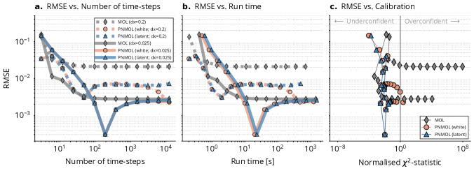
Figure 4: Quantify the global error: Work vs. precision vs. calibration of PNMOL in the latent-force version (blue) and the white-noise version (orange), compared to a traditional PN ODE solver combined with conventional MOL (grey), on the spatial Lotka-Volterra model. Two kinds of curves are shown: one for a coarse (dotted), and one for a fine spatial mesh (solid). A reference is computed by discretising the spatial domain with a ten times finer mesh and solving the ODE with backward differentiation formulas. The RMSE of both methods stagnates once a certain accuracy is reached, but PNMOL appears to reach a slightly lower RMSE for $dx=0.2$ (left, middle; perhaps due to different treatment of boundary conditions; Supplement A). The run time of PNMOL-white is comparable to that of MOL, and the run time of PNMOL-latent is slightly longer (middle). The calibration of PNMOL, measured in the normalised $\chi^{2}$-statistic of the Gaussian posterior (so that the “optimum” is 1, not $d$), remains close to $1$ but is slightly underconfident. With decreasing time-steps, MOL is poorly calibrated.

6 RELATED WORK

Connections to non-probabilistic numerical approximation have been discussed in Sections 2 and 3. Recall from there that the strongest connections are to unsymmetric collocation (Kansa,, 1990; Hon and Schaback,, 2001; Schaback,, 2007), radial-basis-function-generated finite differences (Driscoll and Fornberg,, 2002; Shu et al.,, 2003; Tolstykh and Shirobokov,, 2003; Fornberg and Flyer,, 2015), and collocation methods in general. We refer to Fasshauer, (2007); Fornberg and Flyer, (2015) for a more comprehensive overview. The literature on the method of lines is covered by, e.g., Schiesser, (2012). Dereli and Schaback, (2013); Hon et al., (2014) combine collocation with MOL. None of the above exploits the correlations between spatial and temporal errors. The significance of estimating the interplay of both error sources for MOL has been recognised by Berzins, (1988); Lawson et al., (1991); Berzins et al., (1991).

Cockayne et al., (2017); Owhadi, (2015, 2017); Raissi et al., (2017, 2018) describe a probabilistic solver for PDEs relating to symmetric collocation approaches from numerical analysis. Chen et al., (2021) extend the ideas to non-linear PDEs. Wang et al., (2021) continue the work of Chkrebtii et al., (2016) in constructing an ODE/PDE initial value problem solver that uses (approximate) conjugate Gaussian updating at each time-step. Duffin et al., (2021) solve time-dependent PDEs by discretising the spatial domain with finite elements, and applying ensemble and extended Kalman filtering in time. They build on the paper by Girolami et al., (2021). Conrad et al., (2017); Abdulle and Garegnani, (2021) compute probabilistic PDE solutions by randomly perturbing non-probabilistic solvers. All of the above discard the uncertainty associated with discretising $\mathcal{D}\approx D$. Some papers achieve ODE-solver-like complexity for time-dependent problems (Wang et al.,, 2021; Chkrebtii et al.,, 2016; Duffin et al.,, 2021), while others compute a continuous-time posterior (Cockayne et al.,, 2017; Owhadi,, 2015, 2017; Raissi et al.,, 2017, 2018; Chen et al.,, 2021). PNMOL does both.

The efficiency of the PDE filter builds on recent work on filtering-based probabilistic ODE solvers (Schober et al.,, 2019; Tronarp et al.,, 2019; Kersting et al., 2020b, ; Kersting and Hennig,, 2016; Bosch et al.,, 2021; Krämer and Hennig,, 2020; Tronarp et al.,, 2021) and their applications (Kersting et al., 2020a, ; Schmidt et al.,, 2021). Frank and Enßlin, (2020) apply an ODE filter to solve discretised PDEs. Similar algorithms have been developed for other types of ODEs (Hennig and Hauberg,, 2014; John et al.,, 2019; Krämer and Hennig,, 2021). The papers by Chkrebtii et al., (2016); Conrad et al., (2017); Abdulle and Garegnani, (2020), prominently feature ODEs.

7 EXPERIMENTS

Code

The code for the experiments, and an implementation of the PN discretisation and PN finite differences described in Sections 2 and 3 are on GitHub.

Quantify The Global Error

We investigate how the PN method of lines impacts numerical uncertainty quantification. As a first experiment, we solve a spatial Lotka-Volterra model (Holmes et al.,, 1994), i.e. nonlinear predator-prey dynamics with spatial diffusion, on a range of temporal and spatial resolutions. From the results in Fig. 4, it is evident how the spatial accuracy limits the overall accuracy. But also how traditional ODE filters combined with MOL fail to quantify numerical uncertainty reliably. At any parameter configuration, it is either the spatial or the temporal discretisation that dominates the error. Decreasing the time-step alone lets the error not only stagnate but worsens the calibration because the ODE solver does not know how bad the spatial approximation is.

Which Error Dominates?

To further examine which one of either $\Delta x$ or $\Delta t$ dominates the approximation, we consider a second example: a spatial SIR model (Gai et al.,, 2020). We investigate more formally how increasing either, the time-resolution vs. the space-resolution, leads to a low overall error. The results are in Fig. 5, and confirm the findings from Fig. 4 above.

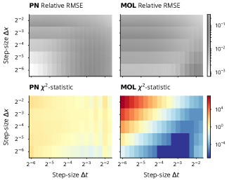
Figure 5: Which error dominates? The relative RMSE is only small if both $\Delta t$ and $\Delta x$ are small, which affects all solvers: PNMOL (top left) as well as traditional MOL combined with PN ODE solvers (top right). PN w/ MOL is severely overconfident for large $\Delta x$ and small $\Delta t$ (bottom right), while PNMOL delivers a calibrated posterior distribution (bottom left).

Traditional PN ODE solvers with conventional MOL are unaware of the true, global approximation error. PNMOL is not, despite being equally accurate.

8 CONCLUSION

We presented probabilistic strategies for discretising PDEs, and for making use of the resulting quantification of spatial discretisation uncertainty in a probabilistic ODE solver. We discussed practical considerations, including sparsification of the differentiation matrices, keeping the dimensionality of the state-space low, and hyperparameter choices. Altogether, and unlike traditional PDE solvers, the probabilistic method of lines unlocks quantification of spatiotemporal correlations in an approximate PDE solution, all while preserving the efficiency of adaptive ODE solvers. This makes it a valuable algorithm in the toolboxes of probabilistic programs and differential equation solvers and may serve as a backbone for latent force models, inverse problems, and differential-equation-centric machine learning.

Acknowledgements

The authors gratefully acknowledge financial support by the German Federal Ministry of Education and Research (BMBF) through Project ADIMEM (FKZ 01IS18052B). They also gratefully acknowledge finan- cial support by the European Research Council through ERC StG Action 757275 / PANAMA; the DFG Cluster of Excellence “Machine Learning - New Perspectives for Science”, EXC 2064/1, project number 390727645; the German Federal Ministry of Education and Re- search (BMBF) through the Tübingen AI Center (FKZ: 01IS18039A); and funds from the Ministry of Science, Research and Arts of the State of Baden- Württemberg. Moreover, the authors thank the Inter- national Max Planck Research School for Intelligent Systems (IMPRS-IS) for supporting Nicholas Krämer.

The authors thank Nathanael Bosch for helpful feed- back on the manuscript.

 

Supplementary Material:
Probabilistic Numerical Method of Lines
for Time-Dependent Partial Differential Equations

 

This supplement explains details regarding: (i) treatment of boundary conditions (Supplement A); (ii) the probabilistic numerical discretisation from Section 2 being a Bayesian probabilistic numerical method (Supplement B); (iii) quasi-maximum-likelihood-estimation of the output-scale $\gamma$ (Supplement C); and (iv) inference schemes for fully non-linear systems of partial differential equations (Supplement D).

Recall the abbreviations from the main paper: partial differential equation (PDE), ordinary differential equation (ODE), probabilistic numerics (PN), method of lines (MOL), probabilistic numerical method of lines (PNMOL).

Appendix A BOUNDARY CONDITIONS

A.1 Setup

In this section, we explain how PNMOL treats boundary conditions. Recall the differential operator $\mathcal{D}$ from Eq. 1, the differentiation matrix $D$ and the error covariance matrix $E$ from Eq. 9, respectively Eqs. 13 and 14. Also recall from Section 4.4 that in the ODE solve, each pair of states $(\vec{U},\vec{\xi})$ is conditioned on a zero PDE residual

$$r(t):=\dot{U}(t)-F(t,{\mathbb{X}},U(t),DU(t)+\xi)\overset{!}{=}0$$ (30)

where $U$, $\dot{U}$, and $\xi$ are components of the extended state vectors $\vec{U}$ and $\xi$. The remainder of this section extends this framework to include boundary conditions $\mathcal{B}u(t,x)=g(x)$ for all $x\in\partial\Omega$ and some function $g$ (Eq. 1).

A.2 Discretised Boundary Conditions

To augment the PDE residual information with boundary conditions, we begin by discretising $\mathcal{B}$ probabilistically; either with global collocation as in Section 2 or with PN finite differences as in Section 3. Below, we show the former, because the latter becomes accessible with the same modifications from Section 3. Let $u_{x}\sim\operatorname{\mathcal{GP}}(0,\gamma^{2}k_{x})$. Defining the differentiation matrix $B$ and the error covariance $R$,

$$B:=(\mathcal{B}k_{x})({\mathbb{X}},{\mathbb{X}})k_{x}({\mathbb{X}},{\mathbb{X}})^{-1},\quad R:=(\mathcal{B}^{2}k_{x})({\mathbb{X}},{\mathbb{X}})-Bk_{x}({\mathbb{X}},{\mathbb{X}})B^{\top},$$ (31)

we have access to boundary conditions: For any $y\in\mathbb{R}^{N+1}$,

$$p((\mathcal{B}u_{x})({\mathbb{X}})\mid u_{x}({\mathbb{X}})=y)\sim\mathcal{N}(By,\gamma^{2}R)$$ (32)

holds. For Dirichlet boundary conditions, $\mathcal{B}$ is the identity, thus $B=I_{N+1}$ is the identity matrix and $R\equiv 0$ is the zero matrix. For Neumann conditions, $B$ is the discretised derivative along normal coordinates, and $R$ is generally nonzero (recall the explanation in Section 5 of the cases in which the error matrix is zero). The derivation surrounding Eq. 32 above suggests how the present framework would deal with boundary conditions that are subject to additive Gaussian noise.

A.3 Latent Force

Define the latent force $\vartheta=\vartheta(t)\sim\operatorname{\mathcal{GP}}(0,\gamma^{2}k_{t}\otimes R)$, which will play a role similar to $\xi$ but for the boundary conditions. $\vartheta$ inherits a stochastic differential equation formulation from $k_{t}$ just like $\xi$ does (recall Lemma 3). Denote the stack of $\vartheta$ and its first $\nu\in\mathbb{N}$ time-derivatives by $\vec{\vartheta}$. Let ${\mathbb{X}}_{B}\subset{\mathbb{X}}$ be the subset of boundary points in ${\mathbb{X}}$. The full information operator (i.e. an extended version of Eq. 30) includes $\left.\mathcal{B}u(t,x)\right|_{\partial\Omega}=g(x)$ as

$$r_{\text{full}}(t):=\begin{pmatrix}\dot{U}(t)-F(t,{\mathbb{X}},U(t),DU(t)+\xi)\\ \mathcal{B}U(t)-g({\mathbb{X}}_{B})-\vartheta(t)\end{pmatrix}\overset{!}{=}0.$$ (33)

$r_{\text{full}}$ depends on $\vec{U}$, $\vec{\xi}$, and $\vec{\vartheta}$. Conditioning $(\vec{U},\vec{\xi},\vec{\vartheta})$ on $r_{\text{full}}(t)=0$ yields a probabilistic PDE solution that knows boundary conditions. Notably, the bottom row in $r_{\text{full}}$ is linear in $\left(\vec{U},\vec{\xi},\vec{\vartheta}\right)$ so there is no linearisation required to enable (approximate) inference.

A.4 Comparison To MOL

Boundary conditions in PNMOL enter through the information operator, i.e. on the same level as the PDE vector field $F$, which is different to conventional MOL: In MOL, one only tracks the state variables in the interior of $\Omega$, i.e. $u(t,{\mathbb{X}}\backslash{\mathbb{X}}_{B})$ because boundary conditions can be inferred from the interior straightforwardly. For Dirichlet conditions, the boundary values are always dictated by $g({\mathbb{X}}_{B})$. Let $\frac{\partial}{\partial n}$ be the directional derivative taken in the direction normal to the boundary $\partial\Omega$. For Neumann conditions, for some small $\lambda>0$, we can approximate

$$\frac{\partial}{\partial n}u(t,x)=\frac{u(t,x)-u(t,x-\lambda n)}{\lambda}\overset{!}{=}g(x).$$ (34)

This viewpoint suggests $u(t,x)=\lambda g(x)+u(t,x-\lambda n)$ and $\lambda$ can be chosen such that $x-\lambda n$ is the nearest neighbor of $x\in{\mathbb{X}}$. While tracking only the state values in the interior of the domain has the advantage that the ODE system emerging from the method of lines is smaller than for PNMOL (which perhaps explains why in Fig. 4, PNMOL achieves a lower error than MOL), MOL has two disadvantages: (i) non-deterministic boundary conditions are not straightforward to include; (ii) the finite difference approximation of Neumann conditions introduces errors. PNMOL does not face the first issue and quantifies the error mentioned by the second issue.

Appendix B DISCRETISATION AS A BAYESIAN PROBABILISTIC NUMERICAL METHOD

Cockayne et al., (2019) introduce a formal definition of Bayesian and non-Bayesian probabilistic numerical methods. More specifically, they define a probabilistic numerical method to be a tuple of an information operator and a belief update operator. A PN method then becomes Bayesian if its output is the pushforward of a specific conditional distribution through the quantity of interest. All of those objects can be derived for the PN discretisation of $\mathcal{D}$. The same is true for the boundary conditions explained in Supplement A but is omitted in the following. The proof of the statement below mirrors the explanation why Bayesian quadrature is a Bayesian PN method in Section 2.2 of the paper by Cockayne et al., (2019).

Proposition 4.

The approximation of $(\mathcal{D}u_{x})({\mathbb{X}})$ with $D$ and $E$ as in Eqs. 7 and 9, using evaluations of $u_{x}$ at a grid, is a Bayesian probabilistic numerical method.

Proof.

The prior measure is the GP prior $\operatorname{\mathcal{GP}}(0,\gamma^{2}k_{x})$ and defined over some separable Banach space of sufficiently differentiable, real-valued functions. The information operator $\mathcal{I}[\varphi]:=\varphi({\mathbb{X}})$ evaluates a function $\varphi$ at the grid ${\mathbb{X}}$. The belief update restricts the prior measure to the set of functions that interpolate $\varphi({\mathbb{X}})$ (this is standard Gaussian process conditioning). The quantity of interest is the derivative $\mathcal{D}u_{x}$, which results in the posterior distribution in Eq. 5. ∎

Appendix C QUASI-MAXIMUM-LIKELIHOOD ESTIMATION OF THE OUTPUT SCALE

Proving the validity of the estimator in Eq. 29 parallels similar statements for similar settings (Tronarp et al.,, 2019; Bosch et al.,, 2021; Krämer and Hennig,, 2021) and consists of two phases: (i) showing that the posterior covariances are of the form $C_{k}=\gamma^{2}\breve{C}_{k}$ for some $\breve{C}_{k}$, $k=0,...,K$; (ii) deriving the maximum likelihood estimators.

To show the first claim, recall the discrete-time transition of $U$ and $\xi$ from Eq. 22 and the information model from Eq. 25. Then, the fully discretised state-space model is

$$\vec{U}(t_{0}) \sim\mathcal{N}(m_{0}\otimes\mathbf{1},\gamma^{2}C_{0}\otimes k_{x}({\mathbb{X}},{\mathbb{X}}))$$ (35a)

$$\vec{\xi}(t_{0}) \sim\mathcal{N}(m_{0}\otimes\mathbf{1},\gamma^{2}C_{0}\otimes E)$$ (35b)

$$\vec{U}(t_{k+1})\mid\vec{U}(t_{k}) \sim\mathcal{N}(\Phi(h_{k})\vec{U}(t_{k}),\gamma^{2}\Sigma_{U}(h_{k}))$$ (35c)

$$\vec{\xi}(t_{k+1})\mid\vec{\xi}(t_{k}) \sim\mathcal{N}(\Phi(h_{k})\vec{\xi}(t_{k}),\gamma^{2}\Sigma_{\xi}(h_{k}))$$ (35d)

$$r(t_{k})\mid\vec{U}(t_{k}),\vec{\xi}(t_{k}) \sim\delta\left(\dot{U}(t_{k})-F(t,{\mathbb{X}},U(t_{k}),DU(t_{k})+\xi(t_{k})).\right)$$ (35e)

All transitions have a process noise that depends multiplicatively on $\gamma^{2}$. The Dirac likelihood is noise-free. Therefore, the posterior covariance depends multiplicatively on $\gamma$ as well (which can be proved by an induction that is identical to the one in Appendix C of the paper by Tronarp et al., (2019)).

To show the second claim, let a linearised observation model be given by

$$r(t_{k})\mid\vec{U}(t_{k}),\vec{\xi}(t_{k}) \sim\delta\left(H\begin{pmatrix}\vec{U}(t_{k})\\ \vec{\xi}(t_{k})\end{pmatrix}+b\right)$$ (36)

for appropriate $H$ and $b$ (which are explained in Supplement D below). Now, the distribution $p(r(t_{k})\mid r(t_{k-1}))$ is Gaussian and thus fully defined by its mean $\mathbb{E}[r(t_{k})]$ and its covariance $\mathbb{C}[r(t_{k})]$. The covariance $\mathbb{C}[r(t_{k})]$ is again of the form $\gamma^{2}\breve{S}_{k}$ for some $\breve{S}_{k}$ because every filtering covariance is, and the information operator is noise-free. Due to the prediction error decomposition (Schweppe,, 1965),

$$p(r(t_{0}),...,r(t_{K})\mid\gamma)=p(r(t_{0})\mid\gamma)\prod_{k=1}^{N}p(r(t_{k})\mid r(t_{k-1}),\gamma).$$ (37)

Recall that the dimension of $r(t_{k})$ is $N+1$ because ${\mathbb{X}}$ consists of $N+1$ grid points. Because everything is Gaussian, the negative log-likelihood (as a function of $x$) decomposes into

$$-\log p(x;r(t_{0}),...,r(t_{K})\mid\gamma)=\frac{1}{2}\left(\sum_{k=0}^{K}\|x-\mathbb{E}[r(t_{k})]\|_{\mathbb{C}[r(t_{k})]^{-1}}^{2}-{(K+1)(N+1)}\log\gamma^{2}\right).$$ (38)

Setting the $\gamma$-derivative of the negative log-likelihood to zero, i.e. maximising it with respect to $\gamma$, yields the MLE from Eq. 29. Overall, the derivation is very similar to those provided by Tronarp et al., (2019); Bosch et al., (2021) for ODE initial value problems, and Krämer and Hennig, (2021) for ODE boundary value problems.

Appendix D FULLY NONLINEAR (WHITE-NOISE) APPROXIMATE INFERENCE

The main paper explained white-noise approximations only using the example of semilinear PDEs.

This section recalls the basic concepts for linear PDEs and the more general case of fully nonlinear PDEs. The latter goes together with an explanation of Taylor-series linearisation of the nonlinear PDE vector field, so it also supports the statements in Section 4.4. The central idea is to regard the PDE vector field $F(t,x,u(t,x),\mathcal{D}u(t,x))$ as a function of $U$ and $\xi$, instead of $u$ and $\mathcal{D}u$, and linearise each non-linearity with a first order Taylor series.

D.1 Linear PDEs

At first, we explain the general idea for a linear PDE

$$F(t,x,u(t,x),\mathcal{D}u(t,x))=Au(t,x)+B\mathcal{D}u(t,x)$$ (39)

for some coefficients $A$ and $B$. If $u$ is scalar-valued, $A$ and $B$ are scalars. If $u$ is vector-valued, $A$ and $B$ are matrices. $\mathcal{D}u=Du+\xi$ allows for recasting the vector field $F$ as a function of $u$ and $\xi$, instead of $u$ and $\mathcal{D}u$,

$$\tilde{F}(t,U(t),\xi(t)):=F(t,{\mathbb{X}},U(t),\xi(t))=AU(t)+BDU(t)+B\xi(t).$$ (40)

Since this equation is linear in $u$ and $\mathcal{D}u$, thus also in $U$ and $\xi$, there is no need for Taylor-series approximation. The linear measurement model emerges as

$$r_{\text{linear}}(t_{k})\mid\vec{U}(t_{k}),\vec{\xi}(t_{k})\sim\delta\left[\dot{U}(t_{k})-AU(t_{k})-BDU(t_{k})-B\xi(t_{k})\right].$$ (41)

If the temporal evolution of $\xi$ is ignored through replacing $k_{t}$ with a white-noise approximation as in Section 4.5, Eq. 41 becomes

$$r_{\text{linear}}(t_{k})\mid\vec{U}(t_{k})\sim\mathcal{N}\left(\dot{U}(t_{k})-AU(t_{k})-BDU(t_{k}),BEB^{\top}\right).$$ (42)

The same principle can be generalised to fully nonlinear problems as follows.

D.2 Nonlinear PDEs

Next, consider a fully nonlinear PDE vector field $F(t,x,u(t,x),\mathcal{D}u(t,x))$. This general setting includes semilinear and quasilinear systems of equations. As before, we discretise the spatial domain using ${\mathbb{X}}$, use $\mathcal{D}u=DU+\xi$, rewrite

$$\tilde{F}(t,U(t),\xi(t)):=F(t,{\mathbb{X}},u(t,{\mathbb{X}}),Du(t,{\mathbb{X}})+\xi(t)),$$ (43)

and infer the solution via $\tilde{F}$. Since $\tilde{F}$ is nonlinear, we have to linearise it before proceeding. Let $\nabla_{U}\tilde{F}$ be the derivative of $\tilde{F}$ with respect to $U$, and $\nabla_{\xi}\tilde{F}$ be its $\xi$-counterpart. We linearise $\tilde{F}$ at some $\eta=(\eta_{U},\eta_{\xi})\in\mathbb{R}^{2(N+1)}$,

$$\tilde{F}(t,U(t),\xi(t)) \approx\tilde{F}(t,\eta_{U},\eta_{\xi})+\nabla_{U}\tilde{F}(t,\eta_{U},\eta_{\xi})(U(t)-\eta_{U})+\nabla_{\xi}\tilde{F}(t,\eta_{U},\eta_{\xi})(\xi(t)-\eta_{\xi})$$ (44)

$$=:H_{U}U(t)+H_{\xi}\xi(t)+b(t).$$ (45)

$\eta_{U}$ and $\eta_{\xi}$ are commonly chosen as the predicted mean of $\xi$ and $U$, which corresponds to extended Kalman filtering (Särkkä and Solin,, 2019). As a result of the linearisation, the information model reads

$$r_{\text{nonlinear}}(t_{k})\mid\vec{U}(t_{k}),\vec{\xi}(t_{k})\sim\delta\left[\dot{U}(t_{k})-H_{U}U(t_{k})-H_{\xi}\xi(t_{k})-b\right],$$ (46)

or, for the white-noise version,

$$r_{\text{nonlinear}}(t_{k})\mid\vec{U}(t_{k})\sim\mathcal{N}\left(\dot{U}(t_{k})-H_{U}U(t_{k})-b,H_{\xi}EH_{\xi}^{\top}\right).$$ (47)

Eqs. 47 and 46 are both linear in the states, and inference is possible with Kalman filtering and smoothing.

Bibliography

- Abdulle and Garegnani, (2020) Abdulle, A. and Garegnani, G. (2020). Random time step probabilistic methods for uncertainty quantification in chaotic and geometric numerical integration. Statistics and Computing, 30(4):907–932.
- Abdulle and Garegnani, (2021) Abdulle, A. and Garegnani, G. (2021). A probabilistic finite element method based on random meshes: A posteriori error estimators and Bayesian inverse problems. Computer Methods in Applied Mechanics and Engineering, 384:113961.
- Alvarez et al., (2009) Alvarez, M., Luengo, D., and Lawrence, N. D. (2009). Latent force models. In AISTATS 2009.
- Bentley and Ottmann, (1979) Bentley, J. L. and Ottmann, T. A. (1979). Algorithms for reporting and counting geometric intersections. IEEE Transactions on Computers, 28(09):643–647.
- Berzins, (1988) Berzins, M. (1988). Global error estimation in the method of lines for parabolic equations. SIAM Journal on Scientific and Statistical Computing, 9(4):687–703.
- Berzins et al., (1991) Berzins, M., Baehmann, P., Flaherty, J., and Lawson, J. (1991). Towards an automated finite element solver for time-dependent fluid-flow problems. The Mathematics of Finite Elements and Application, 7:181–188.
- Bosch et al., (2021) Bosch, N., Hennig, P., and Tronarp, F. (2021). Calibrated adaptive probabilistic ODE solvers. In AISTATS 2021.
- Cash and Psihoyios, (1996) Cash, J. and Psihoyios, Y. (1996). The MOL solution of time dependent partial differential equations. Computers & Mathematics with Applications, 31(11):69–78.
- Chen et al., (2018) Chen, R. T. Q., Rubanova, Y., Bettencourt, J., and Duvenaud, D. K. (2018). Neural ordinary differential equations. In NeurIPS 2018.
- Chen et al., (2021) Chen, Y., Hosseini, B., Owhadi, H., and Stuart, A. M. (2021). Solving and learning nonlinear PDEs with Gaussian processes. Journal of Computational Physics, 447.
- Chkrebtii et al., (2016) Chkrebtii, O. A., Campbell, D. A., Calderhead, B., and Girolami, M. A. (2016). Bayesian solution uncertainty quantification for differential equations. Bayesian Analysis, 11(4):1239–1267.
- Cockayne et al., (2017) Cockayne, J., Oates, C., Sullivan, T., and Girolami, M. (2017). Probabilistic numerical methods for PDE-constrained Bayesian inverse problems. In AIP Conference Proceedings, volume 1853.
- Cockayne et al., (2019) Cockayne, J., Oates, C. J., Sullivan, T. J., and Girolami, M. (2019). Bayesian probabilistic numerical methods. SIAM Review, 61(4):756–789.
- Conrad et al., (2017) Conrad, P. R., Girolami, M., Särkkä, S., Stuart, A., and Zygalakis, K. (2017). Statistical analysis of differential equations: introducing probability measures on numerical solutions. Statistics and Computing, 27(4):1065–1082.
- Dereli and Schaback, (2013) Dereli, Y. and Schaback, R. (2013). The meshless kernel-based method of lines for solving the equal width equation. Applied Mathematics and Computation, 219(10):5224–5232.
- Driscoll and Fornberg, (2002) Driscoll, T. A. and Fornberg, B. (2002). Interpolation in the limit of increasingly flat radial basis functions. Computers & Mathematics with Applications, 43(3-5):413–422.
- Duffin et al., (2021) Duffin, C., Cripps, E., Stemler, T., and Girolami, M. (2021). Statistical finite elements for misspecified models. Proceedings of the National Academy of Sciences, 118(2).
- Evans, (2010) Evans, L. C. (2010). Partial Differential Equations, volume 19. American Mathematical Society.
- Fasshauer, (1997) Fasshauer, G. E. (1997). Solving partial differential equations by collocation with radial basis functions. In Surface Fitting and Multiresolution Methods, pages 131–138. University Press.
- Fasshauer, (1999) Fasshauer, G. E. (1999). Solving differential equations with radial basis functions: multilevel methods and smoothing. Advances in Computational Mathematics, 11(2):139–159.
- Fasshauer, (2007) Fasshauer, G. E. (2007). Meshfree Approximation Methods with MATLAB. World Scientific.
- Fornberg, (1988) Fornberg, B. (1988). Generation of finite difference formulas on arbitrarily spaced grids. Mathematics of Computation, 51(184):699–706.
- Fornberg and Flyer, (2015) Fornberg, B. and Flyer, N. (2015). A Primer on Radial Basis Functions with Applications to the Geosciences. SIAM.
- Frank and Enßlin, (2020) Frank, P. and Enßlin, T. A. (2020). Probabilistic simulation of partial differential equations. arXiv preprint arXiv:2010.06583.
- Gai et al., (2020) Gai, C., Iron, D., and Kolokolnikov, T. (2020). Localized outbreaks in an S-I-R model with diffusion. Journal of Mathematical Biology, 80:1389–1411.
- Gelbrecht et al., (2021) Gelbrecht, M., Boers, N., and Kurths, J. (2021). Neural partial differential equations for chaotic systems. New Journal of Physics, 23(4):043005.
- Girolami et al., (2021) Girolami, M., Febrianto, E., Yin, G., and Cirak, F. (2021). The statistical finite element method (statFEM) for coherent synthesis of observation data and model predictions. Computer Methods in Applied Mechanics and Engineering, 375.
- Hartikainen et al., (2012) Hartikainen, J., Seppänen, M., and Särkkä, S. (2012). State-space inference for non-linear latent force models with application to satellite orbit prediction. ICML 2012.
- Hennig and Hauberg, (2014) Hennig, P. and Hauberg, S. (2014). Probabilistic solutions to differential equations and their application to Riemannian statistics. In AISTATS 2014.
- Holmes et al., (1994) Holmes, E., Lewis, M., Banks, J., and Veit, D. (1994). Partial differential equations in ecology: Spatial interactions and population dynamics. Ecology, 75:17–29.
- Hon and Schaback, (2001) Hon, Y. and Schaback, R. (2001). On unsymmetric collocation by radial basis functions. Applied Mathematics and Computation, 119(2-3):177–186.
- Hon et al., (2014) Hon, Y., Schaback, R., and Zhong, M. (2014). The meshless kernel-based method of lines for parabolic equations. Computers & Mathematics with Applications, 68(12):2057–2067.
- John et al., (2019) John, D., Heuveline, V., and Schober, M. (2019). GOODE: A Gaussian off-the-shelf ordinary differential equation solver. In ICML 2019.
- Kansa, (1990) Kansa, E. J. (1990). Multiquadrics—a scattered data approximation scheme with applications to computational fluid-dynamics—II solutions to parabolic, hyperbolic and elliptic partial differential equations. Computers & Mathematics with Applications, 19(8-9):147–161.
- Kersting and Hennig, (2016) Kersting, H. and Hennig, P. (2016). Active uncertainty calibration in Bayesian ODE solvers. UAI 2016.
- (36) Kersting, H., Krämer, N., Schiegg, M., Daniel, C., Tiemann, M., and Hennig, P. (2020a). Differentiable likelihoods for fast inversion of ’likelihood-free’ dynamical systems. In ICML 2020.
- (37) Kersting, H., Sullivan, T. J., and Hennig, P. (2020b). Convergence rates of Gaussian ODE filters. Statistics and Computing, 30(6):1791–1816.
- Krämer and Hennig, (2020) Krämer, N. and Hennig, P. (2020). Stable implementation of probabilistic ODE solvers. arXiv preprint arXiv:2012.10106.
- Krämer and Hennig, (2021) Krämer, N. and Hennig, P. (2021). Linear-time probabilistic solutions of boundary value problems. In NeurIPS 2021.
- Lawson et al., (1991) Lawson, J., Berzins, M., and Dew, P. M. (1991). Balancing space and time errors in the method of lines for parabolic equations. SIAM Journal on Scientific and Statistical Computing, 12(3):573–594.
- Li et al., (2021) Li, Z., Kovachki, N. B., Azizzadenesheli, K., liu, B., Bhattacharya, K., Stuart, A., and Anandkumar, A. (2021). Fourier neural operator for parametric partial differential equations. In ICLR 2021.
- Lu et al., (2021) Lu, L., Jin, P., Pang, G., Zhang, Z., and Karniadakis, G. E. (2021). Learning nonlinear operators via DeepONet based on the universal approximation theorem of operators. Nature Machine Intelligence, 3:218–229.
- Owhadi, (2015) Owhadi, H. (2015). Bayesian numerical homogenization. Multiscale Modeling & Simulation, 13(3):812–828.
- Owhadi, (2017) Owhadi, H. (2017). Multigrid with rough coefficients and multiresolution operator decomposition from hierarchical information games. SIAM Review, 59(1):99–149.
- Raissi et al., (2017) Raissi, M., Perdikaris, P., and Karniadakis, G. E. (2017). Machine learning of linear differential equations using Gaussian processes. Journal of Computational Physics, 348:683–693.
- Raissi et al., (2018) Raissi, M., Perdikaris, P., and Karniadakis, G. E. (2018). Numerical Gaussian processes for time-dependent and nonlinear partial differential equations. SIAM Journal on Scientific Computing, 40(1):A172–A198.
- Raissi et al., (2019) Raissi, M., Perdikaris, P., and Karniadakis, G. E. (2019). Physics-informed neural networks: A deep learning framework for solving forward and inverse problems involving nonlinear partial differential equations. Journal of Computational Physics, 378:686–707.
- Särkkä and Solin, (2019) Särkkä, S. and Solin, A. (2019). Applied Stochastic Differential Equations. Cambridge University Press.
- Schaback, (1995) Schaback, R. (1995). Error estimates and condition numbers for radial basis function interpolation. Advances in Computational Mathematics, 3(3):251–264.
- Schaback, (2007) Schaback, R. (2007). Convergence of unsymmetric kernel-based meshless collocation methods. SIAM Journal on Numerical Analysis, 45(1):333–351.
- Schiesser, (2012) Schiesser, W. E. (2012). The Numerical Method of Lines: Integration of Partial Differential Equations. Elsevier.
- Schmidt et al., (2021) Schmidt, J., Krämer, N., and Hennig, P. (2021). A probabilistic state space model for joint inference from differential equations and data.
- Schober et al., (2019) Schober, M., Särkkä, S., and Hennig, P. (2019). A probabilistic model for the numerical solution of initial value problems. Statistics and Computing, 29(1):99–122.
- Schweppe, (1965) Schweppe, F. (1965). Evaluation of likelihood functions for Gaussian signals. IEEE Transactions on Information Theory, 11(1):61–70.
- Shu et al., (2003) Shu, C., Ding, H., and Yeo, K. (2003). Local radial basis function-based differential quadrature method and its application to solve two-dimensional incompressible Navier–Stokes equations. Computer methods in applied mechanics and engineering, 192(7-8):941–954.
- Solin, (2016) Solin, A. (2016). Stochastic Differential Equation Methods for Spatio-Temporal Gaussian Process Regression. Doctoral thesis, School of Science.
- Tolstykh and Shirobokov, (2003) Tolstykh, A. and Shirobokov, D. (2003). On using radial basis functions in a “finite difference mode” with applications to elasticity problems. Computational Mechanics, 33(1):68–79.
- Tronarp et al., (2019) Tronarp, F., Kersting, H., Särkkä, S., and Hennig, P. (2019). Probabilistic solutions to ordinary differential equations as non-linear Bayesian filtering: A new perspective. Statistics and Computing, 29(6):1297–1315.
- Tronarp et al., (2021) Tronarp, F., Särkkä, S., and Hennig, P. (2021). Bayesian ODE solvers: The maximum a posteriori estimate. Statistics and Computing, 31(3):1–18.
- Wang et al., (2021) Wang, J., Cockayne, J., Chkrebtii, O., Sullivan, T. J., and Oates, C. J. (2021). Bayesian numerical methods for nonlinear partial differential equations. Statistics and Computing, 31.