Energy-conserving explicit and implicit time integration methods for the multi-dimensional Hermite-DG discretization of the Vlasov-Maxwell equations

Abstract

We study the conservation properties of the Hermite-discontinuous Galerkin (Hermite-DG) approximation of the Vlasov-Maxwell equations. In this semi-discrete formulation, the total mass is preserved independently for every plasma species. Further, an energy invariant exists if central numerical fluxes are used in the DG approximation of Maxwell’s equations, while a dissipative term is present when upwind fluxes are employed. In general, traditional temporal integrators might fail to preserve invariants associated with conservation laws during the time evolution. Hence, we analyze the capability of explicit and implicit Runge-Kutta (RK) temporal integrators to preserve such invariants. Since explicit RK methods can only ensure preservation of linear invariants but do not provide any control on the system energy, we consider modified explicit RK methods in the family of relaxation Runge-Kutta methods (RRK). These methods can be tuned to preserve the energy invariant at the continuous or semi-discrete level, a distinction that is important when upwind fluxes are used in the discretization of Maxwell’s equations since upwind provides a numerical source of energy dissipation that is not present when central fluxes are used. We prove that the proposed methods are able to preserve the energy invariant and to maintain the semi-discrete energy dissipation (if present) according to the discretization of Maxwell’s equations. An extensive set of numerical experiments corroborates the theoretical findings. It also suggests that maintaining the semi-discrete energy dissipation when upwind fluxes are used leads to an overall better accuracy of the method relative to using upwind fluxes while forcing exact energy conservation.

Keyword. 3-D Vlasov-Maxwell equations, Conservation laws, Runge-Kutta temporal integrators, Hermite-Discontinuous Galerkin discretization

1 Introduction

The Vlasov-Maxwell equations for modeling collisionless plasmas in presence of self-consistent electromagnetic fields possess an infinite number of invariants, i.e., quantities that do not change while the physical system evolves in time [15, 1, 3]. These quantities are related to the moments of the particle distribution functions with respect to the independent velocity variable and include terms in their definition that may depend on the electromagnetic fields. Importantly, a few of them express fundamental properties of the physical system such as the conservation of the number of particles, which also entails mass and charge conservation, the conservation of the total momentum and the conservation of the total energy.

Reproducing some (or all) of the conservation properties mentioned above in the discrete setting makes a numerical method very compelling, but at the same time it is a nontrivial task [26]. Indeed, it turns out that for only very few numerical methods we can define discrete invariants that can be calculated from the numerical solution and correspond to the number of particles, the total momentum or the total energy of the physical model.

The majority of the literature on numerical schemes able to preserve key invariants of motion at the fully discrete level has focused on particle-based discretizations. Variational algorithms were introduced in [32, 33, 11] based on least action principles. Energy-conserving time integrators for finite element particle-in-cell discretizations of the Vlasov–Maxwell equations have been recently proposed in [28, 5]. Using the Hamiltonian formulation of some kinetic plasma models, Refs. [22, 39, 30] have focused on the preservation of the phase-space structure, via e.g. symplectic integrators, while ensuring global bounds of the numerical errors of conserved quantities.

In a series of previous works [10, 34, 29], it was shown that the spectral expansion of the plasma distribution function, see also [38], makes it possible to formulate numerical methods for the solution of the kinetic equations that show excellent conservation properties and posses many other desirable properties. Such methods are particularly attractive for problems that involve fluid-kinetic coupling, i.e., the coupling between macroscopic and microscale system dynamics. That is because a suitable choice of the spectral basis makes the fluid-kinetic coupling an intrinsic property of the numerical approximation: the low-order terms of the expansion provide a fluid description of the plasma while additional higher-order terms are able to capture features from the underlying kinetics.

In the present work, we investigate the conservation properties for one such method: the numerical approximation of the system of Vlasov-Maxwell equations provided by the spectral-discontinuous Galerkin method proposed in [29]. The method is based on a spectral expansion in velocity space using asymmetrically-weighted Hermite basis functions and an approximation in physical space using piecewise discontinuous polynomials of a given order. The discontinuous Galerkin (DG) method is also applied to the discretization in space of the time-dependent Maxwell equations. Unlike the work presented in [29], here we treat the fully discrete case and focus on the conservation of the total number of particles and the total energy of the system.

The conservation of the number of particles, which implies mass and charge conservation, is a consequence of the conservative formulation of the method, and holds regardless of the discontinuity of the approximate solution fields. However, the discontinuous nature of the approximate distribution functions and electromagnetic fields plays a major role in the conservation of the total momentum and the total energy. Indeed, the momentum is not conserved and a dissipative term proportional to the square of the jumps of the electromagnetics fields affects the energy conservation when upwind numerical fluxes are used in the discretization of Maxwell’s equations. The total energy is instead conserved when central numerical fluxes are adopted for Maxwell’s equations.

We remark that the work of Ref. [29] does not deal with temporal integration. On the contrary, the present manuscript studies the numerical temporal discretization of the system of ordinary differential equations resulting from the aforementioned DG-Hermite discretization. In particular, we study the effect of time integration on the conservation of mass and energy, i.e., the invariants of the semi-discrete problem. The availability of time discretizations able to satisfy the conservation laws of the continuous or semi-discrete problem is of fundamental importance to ensure numerical solutions that reproduce key physical properties of kinetic models. With this objective in mind, we consider two families of one-step temporal integrators: explicit Runge-Kutta methods and (implicit) Gauss-Legendre methods. First, we show that the implicit Gauss-Legendre schemes are able to preserve both the conserved quantities and the dissipation of the total energy, meaning that the amount of energy dissipated by the fully-discrete scheme equals the temporal approximation of the dissipative term ensuing from the Hermite-DG semi-discrete formulation. Secondly, we study the properties of explicit RK schemes: they ensure the preservation of the number of particles (linear invariant) but do not guarantee any control on the evolution of the total energy. However, in practical implementation of plasma solvers, the explicit schemes are often preferred to the implicit ones despite the superior stability and conservation properties of the latter. The reason is that explicit schemes are computationally cheap, unlike implicit schemes whose computational cost is dominated by the solution of a nonlinear system of equations at each time step. This remark also suggests that the availability of explicit RK methods of arbitrary order able to preserve the conservation and dissipation laws of the continuous or semi-discrete problem could have a significant impact on the efficient solution of kinetic plasma models. We address this issue by resorting to explicit RK methods based on projection. Projection methods, cf. for instance [12, Section 5.3] and [18], belong to the class of extrinsic numerical time integrators and are based on the projection of the numerical solution onto the manifold that is constrained by a given conservation property. The projection methods considered in this work consist in modifying the RK step by suitable scalar factors that depend on the approximate solution and are determined by the given conservation/dissipation law. This approach was originally proposed in [8, pp. 265–266] to derive conservative RK methods. The idea was extended in [9] to a restricted class of fourth-order methods and further developed in [4] via the so-called incremental direction technique (IDT). More recently, an extension of these methods to preserve inner-product norms of the solution has led to the so-called relaxation Runge–Kutta (RRK) methods [27]. We analyze this family of modified RK methods in the context of the Hermite-DG discretization of the Vlasov-Maxwell equations. For the semi-discrete problem considered, this correction guarantees the preservation of the energy invariant and can be tuned to preserve it either at the continuous level, or at the semi-discrete level (this distinction is only relevant when upwind numerical fluxes are used in Maxwell’s equations, since for central fluxes the total energy is conserved at both continuum and semi-discrete levels). With numerical experiments, we show that the latter choice that maintains the semi-discrete energy dissipation when upwind numerical fluxes are used in the discretization of Maxwell’s equations leads to a better overall accuracy of the method relative to a method that uses upwind fluxes but forces exact energy conservation.

The remainder of the paper is organized as follows. In Section 2, we introduce the Vlasov-Maxwell equations as the mathematical model that describes the transport phenomena of different charged particle species in a collisionless plasma under the action of the self-consistent electromagnetic field. Section 3 is devoted to the temporal discretization of the Vlasov-Maxwell equations by using explicit Runge-Kutta methods and implicit Gauss-Legendre methods that are reformulated as a single time-evolution problem. In Section 4, we summarize the space-velocity discretization of the Vlasov-Maxwell equations performed with the Hermite-DG methods introduced in [29]. Next, Section LABEL:sec:invariants pertains to the study of the conservation laws associated with the total number of particles and the total energy and to their characterization as conserved quantities of the ODE resulting from the semi-discrete system of Vlasov-Maxwell equations. In Section LABEL:sec:cons-general, we analyze the capability of Runge-Kutta temporal integrators to preserve the conservative and dissipative relations associated with the different spatial discretizations, and we study modified explicit schemes that preserve mass and total energy of the semi-discrete Vlasov-Maxwell problem. In Section LABEL:sec:numerical:results, we experimentally assess the performance of the proposed methods on the whistler instability test case, on the Orzsag-Tang vortex test case, and in resolving dispersion properties of high frequency waves. Finally, in Section 8 we present some conclusions and final considerations.

Notation and normalization. We normalize the model equations as follows. Time $t$ is normalized to the electron plasma frequency $\omega_{pe}=\sqrt{e^{2}n^{e}_{0}/{}\varepsilon_{0}m^{e}}$, where $e$ is the elementary charge, $m^{e}$ is the electron mass, $\varepsilon_{0}$ is the permittivity of vacuum, and $n^{e}_{0}$ is a reference electron density. The velocity coordinate $v$ is normalized to the speed of light $c$; the spatial coordinate $x$ is normalized to the electron inertial length $d_{e}=c/{\omega_{pe}}$; the magnetic field $\bm{B}$ is normalized to a reference magnetic field $\mathcal{B}_{0}$, and the electric field is normalized to $c\mathcal{B}_{0}$. We denote the quantities associated with a given plasma species by the superscript $s$, which may take the specific values $s=e$ (electrons) and $s=i$ (ions), etc. Accordingly, we denote the mass of the particles of species $s$ by $m^{s}$ and their charge by $q^{s}=\pm e$. We normalize the charge $q^{s}$ and the mass $m^{s}$ to the elementary charge $e$ and the mass $m^{e}$, respectively. Finally, we define the cyclotron frequency of species $s$ as $\omega_{cs}=e\mathcal{B}_{0}/m^{s}$. For simplicity, we maintain the same symbol for each normalized variable and from now on we will only consider normalized quantities.

2 Vlasov-Maxwell equations

The Vlasov-Maxwell equations provide a model for collisionless plasmas [16]. At any time instant $t>0$, the behavior of the particles of species $s$ in the plasma is described by the non-negative distribution function $f^{s}(\bm{x},\bm{v},t)$, where $\bm{x}$ denotes the position in the physical space $\Omega_{x}$ and $\bm{v}$ the position in the velocity space $\Omega_{v}$. The plasma evolves self-consistently under the action of the electric and magnetic fields $\bm{E}(\bm{x},t)$ and $\bm{B}(\bm{x},t)$ generated by particles’ motion (and external sources): the distribution function of species $s$ satisfies the (normalized) Vlasov equation

$$\frac{\partial f^{s}}{\partial t}+\bm{v}\cdot\nabla_{\bm{x}}f^{s}+\frac{q^{s}}{m^{s}}\frac{\omega_{ce}}{\omega_{pe}}\big{(}\bm{E}+\bm{v}\times\bm{B}\big{)}\cdot\nabla_{\bm{v}}f^{s}=0.$$ (1)

Let $\bm{J}$ and $\rho$ denote the self-consistent electric current and charge density, respectively, induced by the plasma particles, namely

$$\rho(\bm{x},t)=\sum_{s=1}^{N_{\text{s}}}q^{s}\int_{\Omega_{v}}f^{s}(\bm{x},\bm{v},t)d\bm{v},\qquad\bm{J}(\bm{x},t)=\sum_{s=1}^{N_{\text{s}}}q^{s}\int_{\Omega_{v}}\bm{v}f^{s}(\bm{x},\bm{v},t)d\bm{v},$$

where $N_{\text{s}}$ denotes the number of plasma species. The electric and magnetic fields $\bm{E}$ and $\bm{B}$ satisfy the time-dependent wave propagation equations

$$\frac{\partial\bm{E}}{\partial t}-\nabla_{\bm{x}}\times\bm{B}=-\frac{\omega_{pe}}{\omega_{ce}}\bm{J},$$ (2)

$$\frac{\partial\bm{B}}{\partial t}+\nabla_{\bm{x}}\times\bm{E}=0,$$ (3)

and the divergence equations

$$\nabla_{\bm{x}}\cdot\bm{E}=\frac{\omega_{pe}}{\omega_{ce}}\rho,$$

$$\nabla_{\bm{x}}\cdot\bm{B}=0.$$

We consider the unbounded velocity space $\Omega_{v}=\mathbbm{R}^{3}$ and we assume that, for $\left|\bm{v}\right|\to\infty$, each distribution function $f^{s}$ decays sufficiently fast, e.g. as $\exp(-\left|\bm{v}\right|^{2})$  [15]. For example, this assumption is physically consistent with near-Maxwellian velocity distribution of a plasma close to thermodynamic equilibrium [17]. Similarly, we consider the closed bounded subset $\Omega_{x}\subset\mathbbm{R}^{3}$ with boundary $\partial\Omega_{x}$, and we assume that suitable problem-dependent boundary conditions for $f^{s}$, $\bm{E}$, and $\bm{B}$ are prescribed at $\partial\Omega_{x}$ for any time $t$ and any $\bm{v}$ in $\Omega_{v}$. Moreover, we consider the plasma evolution in the temporal interval $[0,T]$ and assume that physically meaningful initial conditions are provided for the unknown fields $f^{s}$, $\bm{E}$, $\bm{B}$ at the initial time $t=0$. Since we pursue a numerical approximation of the Vlasov-Maxwell equations based on a spatial discontinuous Galerkin method, we reformulate Eqs. (2)-(3) in conservative form as follows. Let us introduce, for any $t>0$ and $\bm{x}\in\Omega_{x}$, the vector of conservative unknowns $\bm{u}$ and the source term $\bm{S}$,

$$\bm{u}(\bm{x},t):=\left(\begin{array}[]{c}\bm{E}(\bm{x},t)\\[5.0pt] \bm{B}(\bm{x},t)\end{array}\right),\qquad\bm{S}(\bm{x},t)=\left(\begin{array}[]{c}\bm{S}_{\bm{E}}\\[5.0pt] \bm{S}_{\bm{B}}\end{array}\right):=-\frac{\omega_{pe}}{\omega_{ce}}\left(\begin{array}[]{c}\bm{J}(\bm{x},t)\\[5.0pt] \mathbf{0}\end{array}\right),$$ (10)

and the fluxes,

$$\qquad\mathbb{F}(\bm{u}):=\left(\begin{array}[]{c}\mathbb{F}_{\bm{E}}(\bm{u})\\[5.0pt] \mathbb{F}_{\bm{B}}(\bm{u})\end{array}\right),\qquad\nabla_{\bm{x}}\cdot\mathbb{F}(\bm{u})=\left(\begin{array}[]{c}\nabla_{\bm{x}}\cdot\mathbb{F}_{\bm{E}}(\bm{u})\\[5.0pt] \nabla_{\bm{x}}\cdot\mathbb{F}_{\bm{B}}(\bm{u})\end{array}\right)=\left(\begin{array}[]{c}-\nabla_{\bm{x}}\times\bm{B}\\[5.0pt] \nabla_{\bm{x}}\times\bm{E}\end{array}\right),$$ (17)

where the operator $\nabla_{\bm{x}}\,\cdot\,$ denotes here the row-wise divergence in physical space. An explicit form for fluxes $\mathbb{F}$ is given in Section 4.1. With these definitions, Maxwell’s equations (2) and (3) can be written in conservative form as

$$\frac{\partial\bm{u}}{\partial t}+\nabla_{\bm{x}}\cdot\mathbb{F}(\bm{u})={\color[rgb]{0,0,0}\bm{S}(\bm{x},t)}.$$ (18)

3 Temporal discretization of the Vlasov-Maxwell equations

For the numerical approximation of the Vlasov-Maxwell equations, we pursue a method of line approach with Runge-Kutta temporal integrators coupled with the DG-spectral approximation in space-velocity introduced in [29], and summarized in Section 4.

Since the focus of this work is on numerical time integrators, we start by reformulating the Vlasov equation (1) for every plasma species $s$, and the wave propagation equations (2)-(3) as a single time-evolution problem and consider its temporal discretization. To this aim, consider the vector-valued function collecting all the unknowns

$$\mathbf{Y}(\bm{x},\bm{v},t)=\left(\begin{array}[]{c}\big{(}f^{s}(\bm{x},\bm{v},t)\big{)}_{s}\\[5.0pt] \bm{E}(\bm{x},t)\\[5.0pt] \bm{B}(\bm{x},t)\end{array}\right),\qquad t>0,\;\bm{x}\in\Omega_{x},\;\bm{v}\in\Omega_{v},\;s=1,\ldots,N_{\text{s}}\,.$$ (22)

The function $\mathbf{Y}$ satisfies the partial differential equation

$$\dfrac{\partial\mathbf{Y}}{\partial t}=\mathcal{F}(\mathbf{Y};\bm{x},\bm{v},t)\qquad\mbox{in}\quad\Omega_{x}\times\Omega_{v}\times(0,T],$$ (23)

with suitable initial conditions $\mathbf{Y}(\bm{x},\bm{v},0)=\mathbf{Y}_{0}(\bm{x},\bm{v})$, and boundary conditions, as described in Section 2. The operator $\mathcal{F}$ in (23) is defined as

$$\mathcal{F}(\mathbf{Y};\bm{x},\bm{v},t)=\left(\begin{array}[]{c}\big{(}-\bm{v}\cdot\nabla_{\bm{x}}f^{s}-\frac{q^{s}}{m^{s}}\frac{\omega_{ce}}{\omega_{pe}}\big{(}\bm{E}+\bm{v}\times\bm{B}\big{)}\cdot\nabla_{\bm{v}}f^{s}\big{)}_{s}\\[10.00002pt] {\color[rgb]{0,0,0}\bm{S}(\bm{x},t)}-\nabla_{\bm{x}}\cdot\mathbb{F}(\bm{u})\end{array}\right),$$ (26)

where the first term corresponds to the Vlasov equation (1), while the second term is associated with Maxwell’s equations in conservative form (18). The boundary conditions can be introduced in the above setting through additional conditions on the unknown functions $f^{s}$ and $\bm{u}$ or by suitably including them in the discretization in space and velocity that is introduced in Section 4.

For the temporal discretization of problem (23), we split the time integration domain $(0,T]$ into the union of intervals $(t^{\tau},t^{\tau+1}]$, $\tau\in\mathbb{N}_{0}$, with time step $\Delta t^{\tau}=t^{\tau+1}-t^{\tau}$. Let us denote by $\mathbf{Y}^{\tau}(\bm{x},\bm{v})$ the approximation of the function (22) at time $t^{\tau}$, and assume that the initial condition $\mathbf{Y}^{0}(\bm{x},\bm{v})$ is given, for all $\bm{x}\in\Omega_{x}$ and $\bm{v}\in\Omega_{v}$. In the forthcoming formulation of the temporal schemes for (23) we omit, for the sake of better readability, the dependence on the variables $\bm{x}$ and $\bm{v}$. We consider the following two families of approximate one-step temporal integrators:

1. Explicit ${N_{RK}}$-stage Runge-Kutta methods (cf. [20] and references therein).
   The sequence $\{\mathbf{Y}^{\tau}(\bm{x},\bm{v})\}_{\tau}$ of numerical solutions of (23) with initial condition $\mathbf{Y}^{0}$ is obtained as

   $$\mathbf{Y}^{\tau+1}=\varphi_{RK}(\mathbf{Y}^{\tau}) :=\mathbf{Y}^{\tau}+\Delta t^{\tau}\sum_{i=1}^{{N_{RK}}}b_{i}\,\mathcal{F}(\mathcal{Y}_{i}\,;t^{\tau}+c_{i}\Delta t^{\tau}),$$ (27)

   $$\mathcal{Y}_{1} :=\mathbf{Y}^{\tau},$$

   $$\mathcal{Y}_{i} :=\mathbf{Y}^{\tau}+\Delta t^{\tau}\sum_{j=1}^{i-1}a_{ij}\,\mathcal{F}(\mathcal{Y}_{j};t^{\tau}+c_{j}\Delta t^{\tau}),\qquad i=2,\ldots,{N_{RK}}.$$

   The explicit ${N_{RK}}$-stage Runge-Kutta method is, thus, characterized by the Runge-Kutta matrix $(a_{ij})_{1\leq j<i\leq{N_{RK}}}$ and the set of coefficients ${(b_{i})}_{i=1}^{N_{RK}}$, ${(c_{i})}_{i=1}^{N_{RK}}$.

2. Gauss-Legendre methods of order $2{N_{GL}}$ (cf. [21, Chapter IV.5] and references therein).
   Gauss-Legendre temporal integrators are collocation methods based on Gaussian quadrature formulas and belong to the family of implicit Runge-Kutta methods. More specifically, the sequence $\{\mathbf{Y}^{\tau}(\bm{x},\bm{v})\}_{\tau}$ of numerical solutions of (23) with initial condition $\mathbf{Y}^{0}$ is derived as

   $$\mathbf{Y}^{\tau+1}=\varphi_{GL}(\mathbf{Y}^{\tau}) :=\mathbf{Y}^{\tau}+\Delta t^{\tau}\sum_{i=1}^{{N_{GL}}}b_{i}\,\mathcal{F}(\mathcal{Y}_{i}\,;t^{\tau}+c_{i}\Delta t^{\tau}),$$ (28)

   $$\mathcal{Y}_{i} :=\mathbf{Y}^{\tau}+\Delta t^{\tau}\sum_{j=1}^{{N_{GL}}}a_{ij}\,\mathcal{F}(\mathcal{Y}_{j};t^{\tau}+c_{j}\Delta t^{\tau}),\qquad i=1,\ldots,{N_{GL}}\,,$$

   with

   $$a_{ij}:=\int_{0}^{c_{i}}\dfrac{q_{j}(\sigma)}{q_{j}(c_{j})}\,d\sigma,\qquad b_{i}:=\int_{0}^{1}\dfrac{q_{i}(\sigma)}{q_{i}(c_{i})}\,d\sigma,\qquad i,j=1,\ldots,{N_{GL}},$$

   and

   $$q_{i}(\sigma):=\dfrac{\Pi_{j=1}^{{N_{GL}}}(\sigma-c_{j})}{\sigma-c_{i}},\qquad i=1,\ldots,{N_{GL}}.$$

   The Gauss-Legendre method of order $2$ is the implicit midpoint rule. For higher orders, the values of the coefficients $(a_{ij})_{1\leq i,j\leq{N_{GL}}}$, ${(b_{i})}_{i=1}^{N_{GL}}$, and ${(c_{i})}_{i=1}^{N_{GL}}$ in (28) can be found in compendia on numerical methods for ordinary differential equations (ODE), see, e.g., [21, Chapter IV.5].

Throughout, we will adopt the shorthand notation $\mathcal{F}^{N}_{i}:=\mathcal{F}^{N}(\mathcal{Y}_{i};t^{\tau}+c_{i}\Delta t^{\tau})$.

The choice of an explicit or an implicit temporal integrator is dictated by several factors, and it is usually problem-dependent. Explicit methods are computationally attractive since their implementation to solve (23) only requires ${N_{RK}}$ evaluations of the function $\mathcal{F}$ per time step: this allows accurate approximations at a competitive computational cost. However, explicit schemes suffer from time step restrictions due to stability requirements and, as problems become increasingly stiff, implicit methods might become more convenient. Moreover, traditional explicit temporal integrators usually fail to preserve at the discrete level the conservation properties of the continuous system. Indeed such schemes are not even guaranteed to preserve polynomial invariants of degree strictly larger than 1. This might trigger spurious behavior of the approximate problem and yield unphysical solutions, particularly for long-time integration.

Implicit temporal integrators exhibit superior stability properties when compared to explicit schemes. In particular, Gauss-Legendre methods are also symmetric and symplectic, and, hence, are well-suited for the approximation of problems over long temporal intervals. Although the stability properties allow for larger time steps, the implementation costs of implicit methods are dominated by the iterative solvers required for the solution of a nonlinear system of equations at each time step. Therefore, the efficiency of implicit methods strongly relies on the availability of fast linear solvers which, for problems featuring a large number of unknowns, also implies the need for efficient preconditioning strategies. The development of efficient solvers is out of the scope of the present work and might provide an interesting direction for future investigation.

4 Hermite-DG approximation of the Vlasov-Maxwell equations in space and velocity

Concerning the discretization in space and velocity of system (23), we consider the spectral-DG method proposed in [29], where Hermite functions provide the spectral approximation of the Vlasov equation in the velocity space, while a discontinuous Galerkin method is used for the spatial discretization. For reader’s convenience and to introduce the relevant notation, the method described in [29, Section 3] is briefly summarized in this section. Differently from [29], we present the semi-discretization in space and velocity from an equivalent variational formulation perspective.

The spatial domain $\Omega_{x}$ is partitioned into $N_{c}=N_{x}N_{y}N_{z}$ cubic or regular hexahedral cells, with $N_{x}$. $N_{y}$, $N_{z}$ the number of cells in the $x$, $y$, $z$ direction, respectively. We assume that the partition is uniform with mesh size $\Delta x$, $\Delta y$, and $\Delta z$, in each direction, and label the mesh elements by the indices $i,j,k$ running from $1$ to $N_{x}$, $N_{y}$, and $N_{z}$, respectively. For convenience of exposition, the generic mesh cell is labeled by the letter $I$ and the summation over all mesh cells is indicated by $\sum_{I}$, without the summation bounds being specified. With some abuse of notation, we may subindex $I$ as $I_{i,j,k}$. Accordingly, triplets with an half-integer index, e.g. $(i\pm\frac{1}{2},j,k)$, $(i,j\pm\frac{1}{2},k)$ and $(i,j,k\pm\frac{1}{2})$ label the cell interfaces that are orthogonal to the $x$-, $y$-, and $z$-direction, respectively, and delimiting cell $I_{i,j,k}$. With this notation, for example, two consecutive cells in the $x$-direction are denoted by $I_{i,j,k}$ and $I_{i+1,j,k}$ and are separated by the cell interface $\mathsf{f}_{i+\frac{1}{2},j,k}$. The faces are oriented such that the normal vector to each face always points outwards.

For the spatial discretization, we consider multivariate polynomial functions whose restriction to a given mesh cell $I$ is a polynomial of degree at most $N_{DG{}}$. The basis for the local polynomial space $\mathbb{P}_{N_{DG{}}}(I)$ on the mesh element $I$ are denoted by $\{\varphi^{I,l}\}$ for $l=1,\ldots,N_{l}$, so that $\mathbb{P}_{N_{DG{}}}(I)=\mathsf{span}\big{\{}\varphi^{I,l}\}_{l=1}^{N_{l}}$. Here $N_{l}\in\mathbb{N}_{+}$ depends on the polynomial degree $N_{DG{}}$ and on the spatial dimension. We construct the local polynomials $\varphi^{I,l}$ as tensor product of the univariate Legendre polynomials $\{\mathcal{L}_{\zeta}\}_{\zeta=0}^{N_{DG{}}}$ of degree $\zeta$, which are defined in the interval $[-1,1]$ and, then, suitably rescaled and translated on every mesh cell $I$. The polynomials $\mathcal{L}_{\zeta}$ form an orthogonal basis for $\mathbb{P}_{N_{DG{}}}([-1,1])$ [13].

Concerning the spectral approximation in velocity of the Vlasov equation, we consider, as in [29, Section 3.1], the univariate asymmetrically weighted Hermite functions defined as

$$\psi_{\zeta}(\xi^{s}_{\beta})=\big{(}\pi\,2^{\zeta}\,\zeta!\big{)}^{-\frac{1}{2}}\mathcal{H}_{\zeta}(\xi^{s}_{\beta})\exp\big{(}-(\xi^{s}_{\beta})^{2}\big{)},\qquad\psi^{\zeta}(\xi^{s}_{\beta})=\big{(}2^{\zeta}\,\zeta!\big{)}^{-\frac{1}{2}}\mathcal{H}_{\zeta}(\xi^{s}_{\beta}),$$ (29)

where $\mathcal{H}_{\zeta}(\xi^{s}_{\beta})$ is the $\zeta$-th univariate Hermite polynomial in the velocity direction $v_{\beta}$ for $\beta(\zeta)\in\{x,y,z\}$, $\zeta\in\{n,m,p\}$ and $n=0,\ldots,N_{v_{x}}$, $m=0,\ldots,N_{v_{y}}$, $p=0,\ldots,N_{v_{z}}$. Moreover, ${\bm{\xi}}^{s}=\big{(}\xi^{s}_{x},\xi^{s}_{y},\xi^{s}_{z}\big{)}^{T}$, with $\xi^{s}_{\beta}=\frac{v_{\beta}-u^{s}_{\beta}}{\alpha^{s}_{\beta}}$ with the quantities $u^{s}_{\beta}\in\mathbb{R}$ and $\alpha^{s}_{\beta}\in\mathbb{R}$ constant factors that depend on the plasma species (and that are specified by the user). The Hermite functions $\Psi_{n,m,p}$ and $\Psi^{n,m,p}$ are given by the tensor product of the univariate Hermite functions (29) as

$$\Psi_{n,m,p}({\bm{\xi}}^{s})=\psi_{n}(\xi^{s}_{x})\psi_{m}(\xi^{s}_{y})\psi_{p}(\xi^{s}_{z})\quad\textrm{and}\quad\Psi^{n,m,p}({\bm{\xi}}^{s})=\psi^{n}(\xi^{s}_{x})\psi^{m}(\xi^{s}_{y})\psi^{p}(\xi^{s}_{z}).$$

The Hermite-DG variational formulation of the Vlasov-Maxwell system requires the introduction of the following finite dimensional spaces:

$$\mathcal{H}^{N} :=\textrm{span}\Big{\{}\Psi_{n,m,p},\,\textrm{for\leavevmode\nobreak\ }(n,m,p)\in\big{\{}(0,0,0),\ldots,(N_{v_{x}},N_{v_{y}},N_{v_{z}})\big{\}}\Big{\}},$$ (30)

$$\mathcal{\widetilde{H}}^{N} :=\textrm{span}\Big{\{}\Psi^{n,m,p},\,\textrm{for\leavevmode\nobreak\ }(n,m,p)\in\big{\{}(0,0,0),\ldots,(N_{v_{x}},N_{v_{y}},N_{v_{z}})\big{\}}\Big{\}},$$

$$\mathcal{V}^{N} :=\textrm{span}\Big{\{}\bm{\varphi}^{I,l},\,\textrm{for\leavevmode\nobreak\ }I\equiv I_{i,j,k},(i,j,k)\in\big{\{}(1,1,1),\ldots(N_{x},N_{y},N_{z})\big{\}},\,\,l=1,\dots,N_{l}\Big{\}}.$$

4.1 Semi-discrete variational formulation

For any time $t\in[0,T]$, we assume that the numerical distribution function $f^{s,N}(\cdot,\cdot,t)$ belongs to $\mathcal{H}^{N}\times\mathcal{V}^{N}$ for any plasma species $s$ and therefore it can be written as a linear combination of the Hermite and DG basis functions as

$$f^{s,N}(\bm{x},\bm{v},t)=\sum_{n,m,p}\sum_{I,l}C_{n,m,p}^{s,I,l}(t)\Psi_{n,m,p}({\bm{\xi}}^{s})\varphi^{I,l}(\bm{x}),\qquad\forall\,t>0,\,\bm{x}\in\Omega_{x},\,\bm{v}\in\Omega_{v}\,,$$ (31)

where, to ease the notation, we did not specify the summation bounds. Similarly, we take the numerical electromagnetic fields ${\bm{E}}^{N}$ and ${\bm{B}}^{N}$ in the finite-dimensional space $\mathcal{V}^{N}$. Hence, they admit the expansions

$${\bm{E}}^{N}(\bm{x},t) =\sum_{I,l}{\bm{E}}^{I,l}(t)\,\varphi^{I,l}(\bm{x}),\qquad\forall\,t>0,\,\bm{x}\in\Omega_{x}\,,$$ (32)

$${\bm{B}}^{N}(\bm{x},t) =\sum_{I,l}{\bm{B}}^{I,l}(t)\,\varphi^{I,l}(\bm{x}),\qquad\forall\,t>0,\,\bm{x}\in\Omega_{x}\,,$$ (33)

where ${\bm{E}}^{I,l}(t)=\big{(}E_{x}^{I,l}(t),E_{y}^{I,l}(t),E_{z}^{I,l}(t)\big{)}^{T}$ and ${\bm{B}}^{I,l}(t)=\big{(}B_{x}^{I,l}(t),B_{y}^{I,l}(t),B_{z}^{I,l}(t)\big{)}^{T}$ are the DG expansion coefficients of the spatial components of the electric and magnetic fields, ${\bm{E}}^{N}=(E_{x}^{N},E_{y}^{N},E_{z}^{N})^{T}$ and ${\bm{B}}^{N}=(B_{x}^{N},B_{y}^{N},B_{z}^{N})$, respectively.

The semi-discrete variational formulation of the Hermite-DG method reads as: For every species $s$, and any time $t\in(0,T]$, find $f^{s,N}(\cdot,\cdot,t)\in\mathcal{H}^{N}\times\mathcal{V}^{N}$ and ${\bm{E}}^{N}(\cdot,t),{\bm{B}}^{N}(\cdot,t)\in\mathcal{V}^{N}$ such that

$$\mathcal{A}\big{(}(f^{s,N},{\bm{E}}^{N},{\bm{B}}^{N}),(\Psi,\varphi)\big{)} =0\phantom{\mathcal{L}(\varphi)f^{s,N}_{0}{\bm{E}}^{N}_{0}{\bm{B}}^{N}_{0}}\forall\,(\Psi,\varphi)\in\mathcal{\widetilde{H}}^{N}\times\mathcal{V}^{N},$$ (34a)

$$\mathcal{B}\big{(}({\bm{E}}^{N},{\bm{B}}^{N}),\varphi\big{)} =\mathcal{L}(\varphi)\phantom{0f^{s,N}_{0}{\bm{E}}^{N}_{0}{\bm{B}}^{N}_{0}}\forall\,\varphi\in\mathcal{V}^{N},$$ (34b)

$$f^{s,N}(\cdot,\cdot,0) =f^{s,N}_{0}\phantom{0\mathcal{L}(\varphi){\bm{E}}^{N}_{0}{\bm{B}}^{N}_{0}}\textrm{in\leavevmode\nobreak\ }\Omega_{x}\times\Omega_{v}\,,$$ (34c)

$${\bm{E}}^{N}(\cdot,0) ={\bm{E}}^{N}_{0}\phantom{0\mathcal{L}(\varphi)f^{s,N}_{0}{\bm{B}}^{N}_{0}}\textrm{in\leavevmode\nobreak\ }\Omega_{x}\,,$$ (34d)

$${\bm{B}}^{N}(\cdot,0) ={\bm{B}}^{N}_{0}\phantom{0\mathcal{L}(\varphi)f^{s,N}_{0}{\bm{E}}^{N}_{0}}\textrm{in\leavevmode\nobreak\ }\Omega_{x}\,,$$ (34e)

where $$f^{s,N}_{0} {\bm{E}}^{N}_{0} {\bm{B}}^{N}_{0} f^{s}(\cdot,\cdot,0) \bm{E}(\cdot,0) \bm{B}(\cdot,0) \mathcal{H}^{N}\times\mathcal{V}^{N} \mathcal{V}^{N} \mathcal{V}^{N} \partial\Omega_{x}$$, and are the orthogonal projections of the initial conditions , and onto the spaces , and , respectively, and suitable boundary conditions are prescribed on .

To define the multilinear form $\mathcal{A}$ in (34a), we first introduce the auxiliary vector function

$$\bm{g}^{s,N}_{\Psi}(\bm{x},t):=\int_{\Omega_{v}}\bm{v}\,f^{s,N}(\bm{x},\bm{v},t)\Psi({\bm{\xi}})\,d{\bm{\xi}},\quad\forall\,\Psi\in\mathcal{\widetilde{H}}^{N}.$$

Then, for any $f^{s,N}\in\mathcal{H}^{N}\times\mathcal{V}^{N}$, ${\bm{E}}^{N}\in\mathcal{V}^{N}$, ${\bm{B}}^{N}\in\mathcal{V}^{N}$, and $(\Psi,\varphi)\in\mathcal{\widetilde{H}}^{N}\times\mathcal{V}^{N}$, we define

$$\mathcal{A}\big{(}\big{(}f^{s,N},{\bm{E}}^{N},{\bm{B}}^{N}\big{)},(\Psi,\varphi)\big{)}:=\sum_{I}\left(\int_{I}\int_{\Omega_{v}}\dfrac{\partial f^{s,N}}{\partial t}\,\Psi({\bm{\xi}})\,\varphi(\bm{x})\,d{\bm{\xi}}d\bm{x}-\int_{I}\bm{g}^{s,N}_{\Psi}\cdot\nabla_{\bm{x}}\varphi(\bm{x})\,d\bm{x}\right.$$

Concerning the discretization of Maxwell’s equations in (34b), we first consider the fluxes of the conservative formulation (18), and observe that, if we partition the vector flux $\mathbb{F}(\bm{u})$ in a column-wise form, so that

$$\nabla_{\bm{x}}\cdot\mathbb{F}(\bm{u})=\dfrac{\partial}{\partial x}\mathbf{F}_{x}(\bm{u})+\dfrac{\partial}{\partial y}\mathbf{F}_{y}(\bm{u})+\dfrac{\partial}{\partial z}\mathbf{F}_{z}(\bm{u}),$$ (35)

we can write $\mathbf{F}_{x}(\bm{u})=\mathbbm{F}_{x}\bm{u}$, $\mathbf{F}_{y}(\bm{u})=\mathbbm{F}_{y}\bm{u}$, and $\mathbf{F}_{z}(\bm{u})=\mathbbm{F}_{z}\bm{u}$, with flux matrices $\mathbbm{F}_{x},\mathbbm{F}_{y},\mathbbm{F}_{z}\in\mathbb{R}^{6\times 6}$ defined as in [29, Eqs. (50)-(52)]. Let $\bm{n}=(n_{x},n_{y},n_{z})^{T}$ be a generic vector in $\mathbb{R}^{3}$. We use the notation $\mathbb{F}(\bm{u})\bm{n}$ to indicate $\mathbb{F}(\bm{u})\bm{n}:=\mathbf{F}_{x}(\bm{u})n_{x}+\mathbf{F}_{y}(\bm{u})n_{y}+\mathbf{F}_{z}(\bm{u})n_{z}$, and use an analogous definition for $\mathbb{F}_{\bm{E}}(\bm{u})\bm{n}$ and $\mathbb{F}_{\bm{B}}(\bm{u})\bm{n}$. Using [29, Eq. (53)], one has $\mathbb{F}_{\bm{E}}(\bm{u})\bm{n}\cdot\bm{E}=\mathbb{F}_{\bm{B}}(\bm{u})\bm{n}\cdot\bm{B}=\bm{n}\cdot\big{(}\bm{E}\times\bm{B}\big{)}$.

Let $\bm{U}(t):=(({\bm{E}}^{N})^{T},({\bm{B}}^{N})^{T})^{T}$ denote the DG approximation of the vector-valued function $\bm{u}$ in (10). The bilinear form associated with the discretization of Maxwell’s equations is

$$\mathcal{B}\big{(}({\bm{E}}^{N},{\bm{B}}^{N}),\varphi\big{)} :=\mathcal{B}_{\bm{E}}\big{(}({\bm{E}}^{N},{\bm{B}}^{N}),\varphi\big{)}+\mathcal{B}_{\bm{B}}\big{(}({\bm{E}}^{N},{\bm{B}}^{N}),\varphi\big{)},\qquad\qquad\forall\,{\bm{E}}^{N},\,{\bm{B}}^{N},\,\varphi\in\mathcal{V}^{N},$$ (36)

where Figure 6: X mode test: relative error in the conservation of the total energy (top left); wave spectrum computed from $E_{y}(\bm{x},t)$ for methods with central fluxes, i.e., IMC (top right), RKC (bottom left), and MRKC (bottom right).

Figure 7: X mode test: wave spectrum computed from $E_{y}(\bm{x},t)$ for methods with upwind fluxes, i.e., IMU (top left), RKU (top right), MRKU0 (bottom left), and MRKU1 (bottom right).

7.3 Orszag-Tang vortex

In the last test, we investigate the performance of the proposed methods in conserving the total energy when solving the Orszag-Tang vortex problem. In the Orszag-Tang vortex problem [35], two large-scale vortices are initialized and evolve by forming smaller and smaller current sheets and other filamentary structures. In collisionless plasma, the Orszag-Tang initial conditions lead to development of turbulence via breaking (reconnection) of the current sheet formed by the initial evolution [see e.g. 36]. The overall energy dissipation in such a case is thought to be dominated by kinetic effects that become significant at small scales [see e.g. 40, and references therein]. Therefore, this test is an example of the complex, multi-scale problem involving transition between the large-scale, fluid-like behavior of the plasma and the small-scale, dissipative processes involving kinetic physics.

We consider temporal and spatial discretizations with different resolutions: in particular, the time steps $\Delta t\in\{0.05,0.025\}$, and DG polynomial spaces $N_{DG}=1$ (linear) and $N_{DG}=2$ (quadratic). All other numerical parameters and initial conditions are fixed and are outlined below. The computational domain in physical space is two dimensional ($N_{z}=1$) with $\Omega_{x}=[0,L_{x}]\times[0,L_{y}]$, $L_{x}=L_{y}=50$, and periodic boundary conditions. It is discretized with a uniform grid with $N_{x}=N_{y}=108$ elements. We set $N_{v_{x}}=N_{v_{y}}=N_{v_{z}}=3$ for the velocity Hermite expansion. The initial magnetic field is set to

$$B_{x}(\bm{x}) =-\delta B\sin(k_{y}y+4.1),$$

$$B_{y}(\bm{x}) =\delta B\sin(2k_{x}x+2.3),$$

$$B_{z}(\bm{x}) =1,$$

with $\delta B=0.2$, $k_{x}=2\pi/L_{x}$, $k_{y}=2\pi/L_{y}$. The values $4.1$ and $2.3$ are arbitrary phases that remove any artificial symmetry in the initial setup. The distribution functions for electrons and ions are initialized to be shifted Maxwellian distributions with spatially uniform density (species superscripts are omitted for clarity),

$$f(\bm{x},\bm{v},t)=\prod_{\beta\in\{x,y,z\}}\frac{1}{v_{T_{\beta}}\sqrt{2\pi}}\exp\left[-\frac{(v_{\beta}-U_{\beta}(\bm{x}))^{2}}{2v_{T_{\beta}}^{2}}\right],$$

with electron and ion velocities

$$U^{e}_{x}(\bm{x}) =U^{i}_{x}(\bm{x})=-\delta Bv_{a}\sin(k_{y}y+0.5),$$

$$U^{e}_{y}(\bm{x}) =U^{i}_{y}(\bm{x})=\delta Bv_{a}\sin(k_{x}x+1.4),$$

$$U^{e}_{z}(\bm{x}) =-\frac{\delta B\omega_{ce}}{\omega_{pe}}\left(2k_{x}\cos(2k_{x}x+2.3)+k_{y}\cos(k_{y}y+4.1)\right),$$

$$U^{i}_{z}(\bm{x}) =0,$$

where $v_{a}=0.1$ and $\omega_{pe}/\omega_{ce}=2$. The values $0.5$ and $1.4$ are random phases and $U_{z}^{e}$ was chosen to satisfy Ampère’s law at time $t=0$. Other parameters include $m_{i}/m_{e}=25$ and the artificial collision rate $\nu=1$. The species-dependent parameters used in the definition of the Hermite functions are set as follows: $\alpha_{\beta}^{e}=\sqrt{2}v_{T_{\beta}}^{e}=0.25$, $u_{\beta}^{e}=0$ and $\alpha_{\beta}^{i}=\sqrt{2}v_{T_{\beta}}^{e}/\sqrt{m_{i}/m_{e}}=0.05$, $u_{\beta}^{i}=0$ with $\beta\in\{x,y,z\}$.

Similarly to the previous numerical tests, we study the seven methods summarized in Table LABEL:tab:methods. As a qualitative measure of the performances of the proposed methods, we report in Fig. 7.3 the plasma current along the $z$-axis at the final simulation time $t=1000$. All runs with $N_{DG}=2$ (third and fourth columns) show visually indistinguishable solutions. We note that further increasing the temporal, spatial, or velocity resolution does not lead to visible changes in the results (more refined runs are not reported here). All runs with $N_{DG}=1$ (first and second columns), except for the MRKU0 method, produce qualitatively similar plots, but slightly smeared due to the spatial discretization error. The MRKU0 method with $N_{DG}=1$ (sixth row, first and second columns) produce results polluted by high amplitude oscillations, which make the results unreliable. The nature of those oscillations could be related to the unphysical modes which were present in the X-mode test in the previous section, see the bottom left panel of Fig. 4.1.

Figure 8: Orszag-Tang vortex benchmark: out of plane current at $t=1000$ for IMC (first row), RKC (second row), MRKC (third row), IMU (fourth row), RKU (fifth row), MRKU0 (sixth row), MRKU1 (seventh row) with $N_{DG}=1$ (first and second column), $N_{DG}=2$ (third and fourth column), $\Delta t=0.05$ (first and third column), $\Delta t=0.025$ (second and fourth column).

Concerning the energy conservation in the Orszag-Tang vortex test, we distinguish the case of central fluxes in the spatial approximation of Maxwell’s equations (Fig. 9) and upwind fluxes (Fig. 10). The results for central fluxes are similar to the results obtained with the same numerical methods in the whistler instability test in Fig. LABEL:fig:whistler_x:central:energy. In the left panel of Fig. 9, the error in the conservation of energy for the IMC scheme is shown: energy is conserved up to the nonlinear solver tolerance. The middle panel illustrates the performances of the RKC scheme, where the error in the energy conservation depends on the accuracy of the temporal discretization (the error is independent on $N_{DG}$ and scales as the Runge-Kutta order producing a reduction of the error by a factor of $\sim 8=2^{3}$ shown with the two sided black arrow). The right panel shows the results obtained with the MRKC scheme, which confirm that the conservation of energy is satisfied to machine precision.

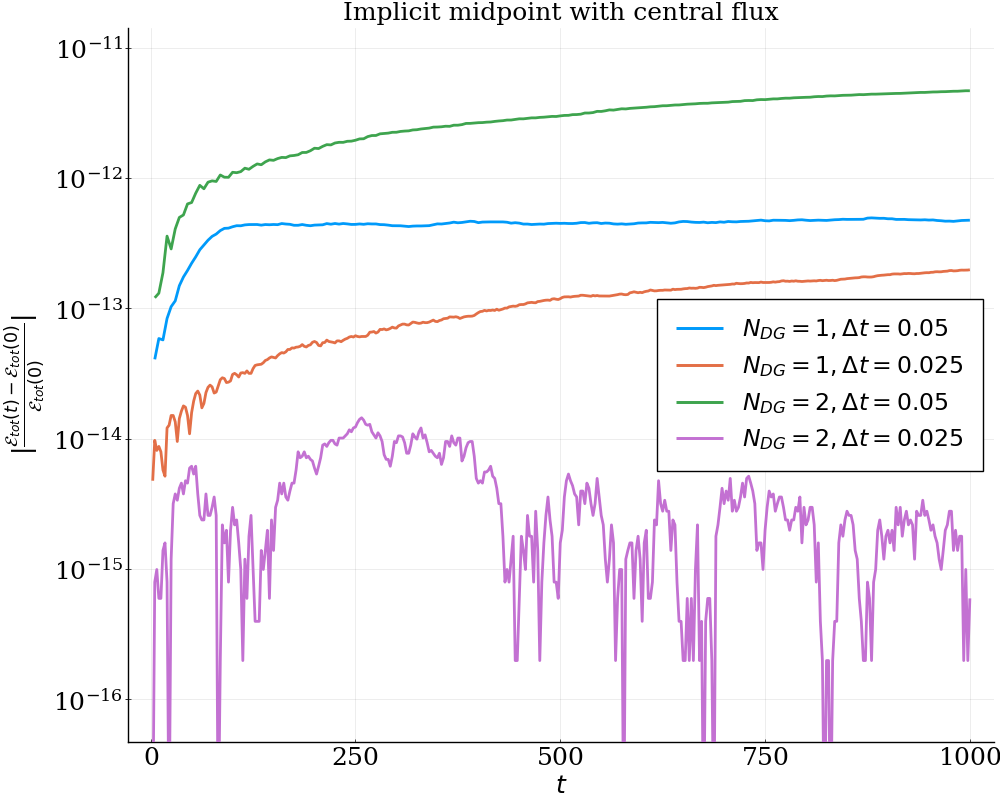
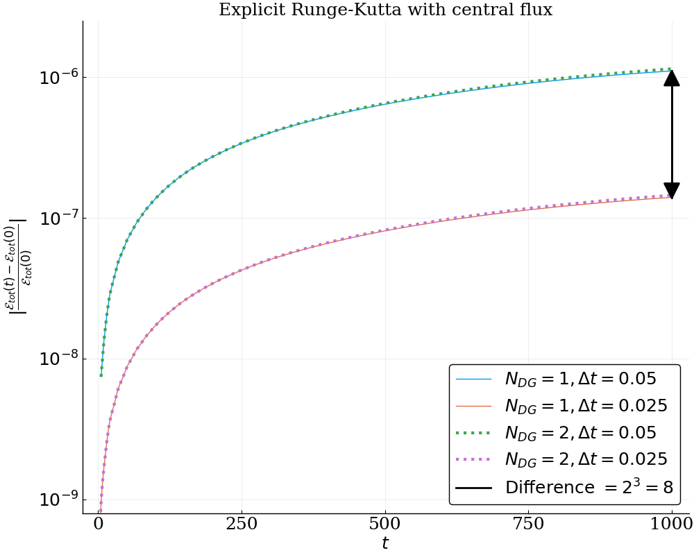
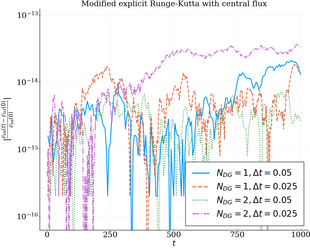
Figure 9: Orszag-Tang vortex benchmark: time evolution of relative error in energy conservation for IMC (left), RKC (middle), and MRKC (right) for different spatial and temporal resolution.

The results for the methods based on upwind fluxes are shown in Fig. 10, and are similar to the ones obtained in the whistler instability test in Fig. LABEL:fig:whistler_x:upwind:energy. The MRKU0 method (left panel) conserves the energy to machine precision although the plot of the current in Fig. 7.3 shows unsatisfactory results (at least for $N_{DG}=1$). All other upwind methods, i.e., IMU, RKU, MRKU1 dissipate energy. The middle panel of Fig. 10 has results with $N_{DG}=1$ and the right panel has $N_{DG}=2$. As before, the effect of the temporal discretization is small compared to the spatial discretization error for $N_{DG}=1$ and the curves associated with different methods and different $\Delta t$ coincide. For $N_{DG}=2$ (right panel), the energy error in some of the methods differ for $t<400$. In general, RKU has an energy error that is one to two orders of magnitude larger than that of IMU and MRKU1, showing that in this case the correction for upwind based Runge-Kutta methods is important. The correct third order scaling of RKU is also recovered, as shown by comparing the curves with $\Delta t=0.05$ and $\Delta t=0.025$. The energy errors for IMU and MRKU1 essentially coincide, irrespective of $\Delta t$. For $t>400$, the energy error becomes dominated by the spatial discretization error and all the curves essentially overlap (cf. Fig. LABEL:fig:whistler_x:upwind:energy).

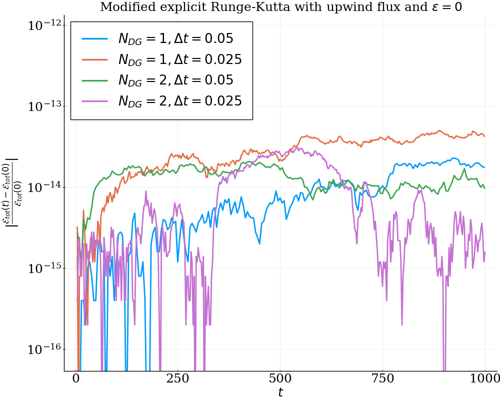
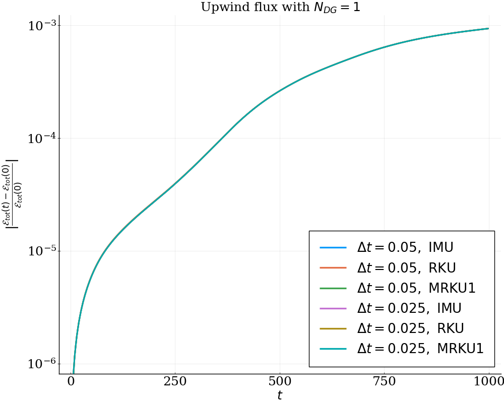
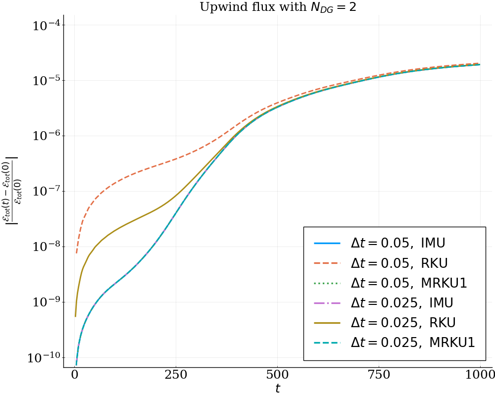
Figure 10: Orszag-Tang vortex benchmark: time evolution of relative error in energy conservation for MRKU0 (left), IMU, RKU, MRKU1 with $N_{DG}=1$ (middle), and IMU, RKU, MRKU1 with $N_{DG}=2$ (right), for different resolution.

Finally, we look at how the electromagnetic energy $\mathcal{E}_{\bm{E},\bm{B}}$ defined in (LABEL:eq:calEBE) changes over time for various methods. The evolution of the electromagnetic energy for runs with $N_{DG}=2$ looks essentially identical for all methods and time steps (not shown here). Therefore, we use a run with $N_{DG}=2$, $\Delta t=0.025$ and the IMC method as a reference in the following results. The left panel in Fig. 11 shows the evolution of $\mathcal{E}_{\bm{E},\bm{B}}$ for runs with central flux and $N_{DG}=1$. One can see that the central flux based methods reproduce the correct dynamics of the electromagnetic energy (as seen by comparing them against the more resolved reference solution). At the same time, IMU, RKU, and MRKU1 with $N_{DG}=1$ consistently dissipate electromagnetic energy for different time step sizes, as shown in the middle panel in Fig. 11. The right panel in Fig. 11 shows the evolution of $\mathcal{E}_{\bm{E},\bm{B}}$ for the MRKU0 method with $N_{DG}=1$. This method conserves the total energy but it overestimates the energy stored in the electromagnetic field. This additional energy is probably related to the unphysical small scale fluctuations observed in the current plots in Fig. 7.3.

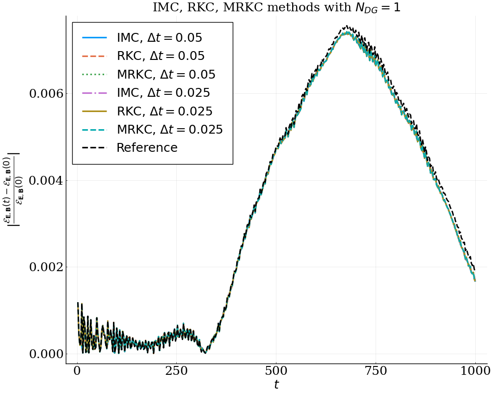
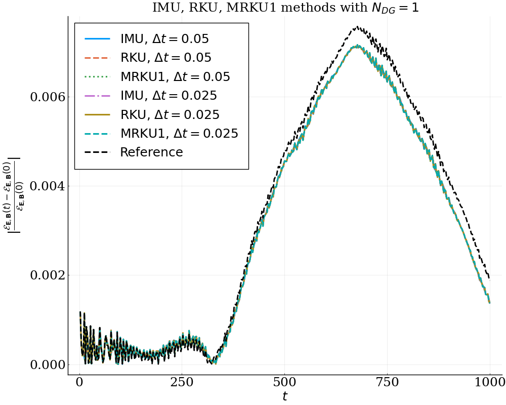
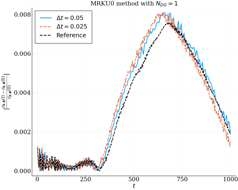
Figure 11: Orszag-Tang vortex benchmark: time evolution of relative change in electromagnetic energy $\mathcal{E}_{\mathbf{E},\mathbf{B}}$ for $N_{DG}=1$ and IMC, RKC, MRKC (left), IMU, RKU, MRKU1 (middle), MRKU0 (right), for different $\Delta t$ against reference solution (IMC with $N_{DG}=2$, $\Delta t=0.025$).

7.4 Notes on momentum conservation and positivity

The total momentum is a conserved quantity of the Vlasov-Maxwell system at the continuum and for periodic boundary conditions. However, as shown in [29, Theorem 5.2], the Hermite-DG discretization of the problem does not exactly conserve the discrete total momentum. If the solution fields are sufficiently regular, the error in the conservation of the discrete momentum decreases according to the order of the semi-discrete approximation. In this section we show that, once we introduce a discretization in time, such violation of the momentum conservation is independent of the temporal integrator. We consider the discrete total momentum defined as

$$P=\sqrt{P_{x}^{2}+P_{y}^{2}+P_{z}^{2}},$$

where

$$P_{x}=\sum_{I,l}\left(\int_{I}\left|\varphi^{I,l}(\bm{x})\right|^{2}d\bm{x}\right)\left(\left(\frac{\omega_{ce}}{\omega_{pe}}\right)^{2}\left(E_{y}^{I,l}B_{z}^{I,l}-B_{y}^{I,l}E_{z}^{I,l}\right)+\sum_{s}m^{s}\alpha_{x}^{s}\alpha_{y}^{s}\alpha_{z}^{s}\left(u_{x}^{s}C^{s,I,l}_{0,0,0}+\frac{\alpha_{x}^{s}}{\sqrt{2}}C^{s,I,l}_{1,0,0}\right)\right),$$

and $P_{y}$ and $P_{z}$ are defined similarly. Figure 12 shows the evolution of the discrete total momentum (the initial momentum is zero) for different test cases and temporal integrators. The left panel shows results for the whistler instability test with $N_{DG}=1$ and $\Delta t=0.01$, where the error in the explicit methods is of the order of machine precision and in the implicit method is of the order of the tolerance of the nonlinear solver. The middle panel shows results for the high frequency electromagnetic waves test, where the error is essentially independent of the time integration strategy. The right panel shows results for the OT test with $N_{DG}=2$ and $\Delta t=0.025$, where the error is also independent of the time integration strategy.

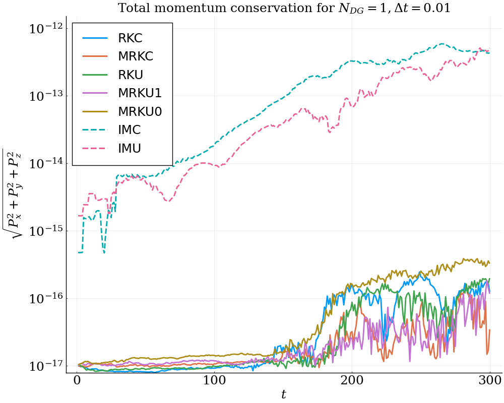
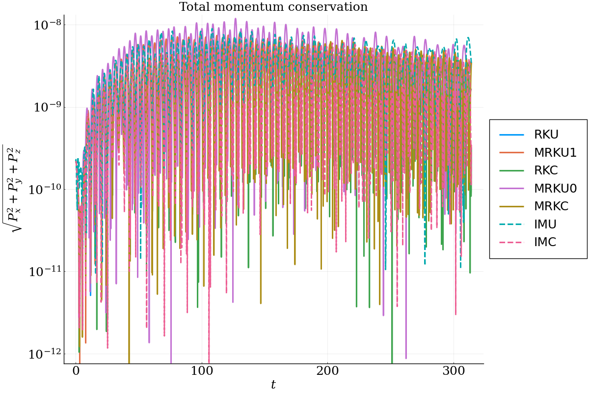
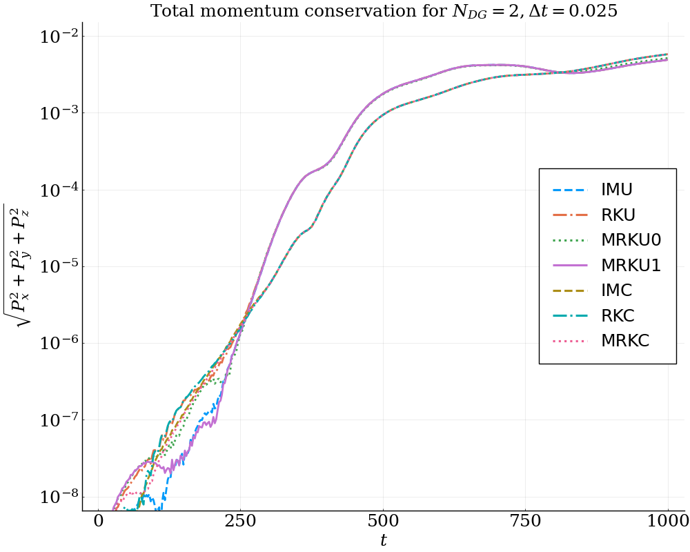
Figure 12: Time evolution of total momentum for different time integration strategies for: whistler instability test with $N_{DG}=1$ and $\Delta t=0.01$ (left); high frequency electromagnetic waves test (middle); OT test with $N_{DG}=2$ and $\Delta t=0.025$ (right).

Another important issue, common to spectral methods, is that the positivity of the distribution function is not guaranteed in the method considered. As an example, in the most difficult test studied in the paper (the OT test), the reconstructed distribution function has regions with negative values for sufficiently large velocities, whose magnitude at late times and at $v>3v_{T}$ (where $v_{T}$ is the thermal velocity) is $\sim 2$% of the (positive) peak value. The error associated with the lack of positivity of the distribution function is fairly insensitive to the time discretization strategy.

We note that the algorithm presented here can be considered as a reduced kinetic model where the distribution function is typically represented with only a few polynomials per velocity direction ($4$ in the OT test). The negativity of the reconstructed distribution function at some values of the velocity has no obvious consequences for the algorithm, as long as it does not introduce significant errors in the first $N_{v}$ moments of the distribution. Additionally, adding more Hermite moments mitigates the positivity problem effectively.

8 Conclusions

We presented the analysis of the conservation properties of the fully-discrete numerical approximation of the Vlasov-Maxwell equations provided by the spectral-discontinuous Galerkin method proposed in [29]. Here the velocity space of the Vlasov equation is expanded in asymmetrically weighted Hermite functions while the spatial part of the Vlasov equation and Maxwell’s equations are discretized with the DG method. The number of particles is conserved in the semi-discrete formulation of the method, while the total energy is conserved if Maxwell’s equations are discretized with central fluxes and dissipates when upwind fluxes are used. Such conservation and dissipation properties are maintained at the fully discrete level by (implicit) Gauss-Legendre temporal integrators but not by explicit Runge-Kutta schemes. Hence, we have adopted modified RK schemes, known as incremental direction techniques (IDT) [4] and relaxation Runge-Kutta methods (RRK) [27], and analyzed them in the context of the Hermite-DG discretization of the Vlasov-Maxwell equations. These are explicit Runge-Kutta methods that maintain the properties of the semi-discrete system by applying a correction step to the regular Runge-Kutta algorithm. The idea behind the method is to tie the correction step to the conservation of a particular quantity (the total energy in this case).

For upwind fluxes in Maxwell’s equations, which provide numerical energy dissipation associated with the DG jumps at the cell interfaces, one might be tempted to apply the Runge-Kutta correction step in a way that forces exact conservation of the total energy (i.e. the conservation property of the system at the continuum level and not at the semi-discrete level). Indeed, we have tested this possibility numerically [Eq. (LABEL:eq:gamma:def) with $\varepsilon=0$, scheme MRKU0 in Table 1] against an approach where the correction step is chosen to preserve the upwind energy dissipation [Eq. (LABEL:eq:gamma:def) with $\varepsilon=1$, scheme MRKU1 in Table 1; this is equivalent to enforcing energy conservation at the semi-discrete level such that to preserve upwind energy dissipation]. In all our numerical experiments, MRKU0 consistently showed lower accuracy of the overall solution relative to MRKU1 when used in conjunction with linear polynomials ($N_{DG}=1$) for DG. For instance, in the Orszag-Tang decaying turbulence test, Fig. 7.3, one can see spurious oscillations in the MRKU0 solution (sixth row, first two columns) that are not present in any of the other methods. These oscillations disappear when one increases the order of the spatial discretization ($N_{DG}=2$, sixth row, third and fourth columns in Fig. 7.3). These results suggest that preserving the properties of the semi-discrete formulation of the method at the fully-discrete level and controlling the numerical dissipation through the accuracy of the spatial discretization might provide a better algorithm when upwind fluxes are used in Maxwell’s equations. For central fluxes, the total energy is a conserved quantity of the evolution problem ensuing from the Hermite-DG discretization since the terms associated with the jumps at cell interfaces disappear. In this case, the modified RK scheme ensures energy conservation at the fully-discrete level.

In closing, we note that explicit time integrators that can conserve energy at the discrete level, such as those discussed in this paper, are very important for plasma physics applications since these methods are much less computationally expensive than the implicit time integrators that also typically can conserve energy. Depending on the application, implicit methods might still be preferable for their overall better numerical stability. Future work might seek the development of energy-conserving semi-implicit methods that combine the advantages of the two classes of schemes and achieve energy conservation in the discrete, while relaxing the computational cost of fully-implicit schemes (as done recently in the area of Particle-In-Cell methods [31]).

Declarations

Funding. The work of GLD, OK, GM was supported by the Laboratory Directed Research and Development - Exploratory and Research (LDRD-ER) Program of Los Alamos National Laboratory under project number 20170207ER. Los Alamos National Laboratory is operated by Triad National Security, LLC, for the National Nuclear Security Administration of U.S. Department of Energy (Contract No. 89233218CNA000001). Computational resources for the SPS-DG simulations were provided by the Los Alamos National Laboratory Institutional Computing Program.

VR’s contributions were supported by DOE grant DE-SC0019315.

Data availability statement. Data sharing not applicable to this article as no datasets were generated or analysed during the current study.

References

- [1] J. A. Bittencourt. Fundamentals of Plasma Physics. Springer-Verlag New York, 2004.
- [2] P. Bogacki and L. F. Shampine. A 3 (2) pair of Runge-Kutta formulas. Applied Mathematics Letters, 2(4):321–325, 1989.
- [3] T. J. M. Boyd and J. J. Sanderson. The Physics of Plasmas. Cambridge University Press, 2003.
- [4] M. Calvo, D. Hernández-Abreu, J. Montijano, and L. Rández. On the preservation of invariants by explicit Runge–Kutta methods. SIAM Journal on Scientific Computing, 28(3):868–885, 2006.
- [5] M. Campos Pinto, K. Kormann, and E. Sonnendrücker. Variational framework for structure-preserving electromagnetic particle-in-cell methods. J. Sci. Comput., 91(2):Paper No. 46, 39, 2022.
- [6] C. Z. Cheng and G. Knorr. The integration of the Vlasov equation in configuration space. Journal of Computational Physics, 22(3):330 – 351, 1976.
- [7] G. J. Cooper. Stability of Runge-Kutta methods for trajectory problems. IMA J. Numer. Anal., 7(1):1–13, 1987.
- [8] K. Dekker and J. G. Verwer. Stability of Runge-Kutta methods for stiff nonlinear differential equations, volume 2 of CWI Monographs. North-Holland Publishing Co., Amsterdam, 1984.
- [9] N. Del Buono and C. Mastroserio. Explicit methods based on a class of four stage fourth order Runge–Kutta methods for preserving quadratic laws. Journal of Computational and Applied Mathematics, 140(1):231–243, 2002. Int. Congress on Computational and Applied Mathematics 2000.
- [10] G. L. Delzanno. Multi-dimensional, fully-implicit, spectral method for the Vlasov-Maxwell equations with exact conservation laws in discrete form. Journal of Computational Physics, 301:338–356, 2015.
- [11] James W. Eastwood. The virtual particle electromagnetic particle-mesh method. Computer Physics Communications, 64(2):252–266, 1991.
- [12] E. Eich-Soellner and C. Führer. Numerical methods in multibody dynamics. European Consortium for Mathematics in Industry. B. G. Teubner, Stuttgart, 1998.
- [13] D. Funaro. Polynomial approximation of differential equations, volume 8. Springer Science & Business Media, 2008.
- [14] S. P. Gary. Theory of space plasma microinstabilities. Cambridge University Press, 2005.
- [15] R. T. Glassey. The Cauchy problem in kinetic theory, volume 52. SIAM, 1996.
- [16] R. J. Goldston and P. H. Rutherford. Introduction to Plasma Physics. CRC Press, 1995.
- [17] H. Grad. On the kinetic theory of rarefied gases. Communications on Pure and Applied Mathematics, 2(4):331–407, 1949.
- [18] V. Grimm and G. R. W. Quispel. Geometric integration methods that preserve Lyapunov functions. BIT, 45(4):709–723, 2005.
- [19] E. Hairer, C. Lubich, and G. Wanner. Geometric numerical integration. Structure-preserving algorithms for ordinary differential equations, volume 31 of Springer Series in Computational Mathematics. Springer, Heidelberg, 2010.
- [20] E. Hairer, S. P. Nørsett, and G. Wanner. Solving ordinary differential equations I. Nonstiff problems, volume 8 of Springer Series in Computational Mathematics. Springer-Verlag, Berlin, second edition, 1993.
- [21] E. Hairer and G. Wanner. Solving ordinary differential equations II. Stiff and differential-algebraic problems, volume 14 of Springer Series in Computational Mathematics. Springer-Verlag, Berlin, 2010.
- [22] Y. He, Y. Sun, J. Liu, and H. Qin. Volume-preserving algorithms for charged particle dynamics. Journal of Computational Physics, 281:135–147, 2015.
- [23] J. S. Hesthaven and T. Warburton. High–order nodal discontinuous Galerkin methods for the Maxwell eigenvalue problem. Philosophical Transactions of the Royal Society of London. Series A: Mathematical, Physical and Engineering Sciences, 362(1816):493–524, 2004.
- [24] A. Iserles. A first course in the numerical analysis of differential equations. Cambridge Texts in Applied Mathematics. Cambridge University Press, Cambridge, 1996.
- [25] G. Joyce, G. Knorr, and H. K. Meier. Numerical integration methods of the Vlasov equation. Journal of Computational Physics, 8(1):53–63, 1971.
- [26] J. Juno, A. Hakim, J. TenBarge, E. Shi, and W. Dorland. Discontinuous Galerkin algorithms for fully kinetic plasmas. Journal of Computational Physics, 353:110–147, 2018.
- [27] D. I. Ketcheson. Relaxation Runge-Kutta methods: conservation and stability for inner-product norms. SIAM J. Numer. Anal., 57(6):2850–2870, 2019.
- [28] K. Kormann and E. Sonnendrücker. Energy-conserving time propagation for a structure-preserving particle-in-cell vlasov–maxwell solver. Journal of Computational Physics, 425:109890, 2021.
- [29] O. Koshkarov, G. Manzini, G. L. Delzanno, C. Pagliantini, and V. Roytershteyn. The multi-dimensional Hermite-discontinuous Galerkin method for the Vlasov–Maxwell equations. Computer Physics Communications, 264:107866, 2021.
- [30] M. Kraus, K. Kormann, P. J. Morrison, and E. Sonnendrücker. Gempic: geometric electromagnetic particle-in-cell methods. Journal of Plasma Physics, 83(4):905830401, 2017.
- [31] G. Lapenta. Exactly energy conserving semi-implicit particle in cell formulation. Journal of Computational Physics, 334:349–366, 2017.
- [32] H. R. Lewis. Energy-conserving numerical approximations for vlasov plasmas. Journal of Computational Physics, 6(1):136–141, 1970.
- [33] H. R. Lewis. Variational algorithms for numerical simulation of collisionless plasma with point particles including electromagnetic interactions. Journal of Computational Physics, 10(3):400–419, 1972.
- [34] G. Manzini, G. L. Delzanno, J. Vencels, and S. Markidis. A Legendre-Fourier spectral method with exact conservation laws for the Vlasov-Poisson system. Journal of Computational Physics, 317:82–107, 2016.
- [35] S. A. Orszag and C.-M. Tang. Small-scale structure of two-dimensional magnetohydrodynamic turbulence. Journal of Fluid Mechanics, 90(1):129–143, 1979.
- [36] T. N. Parashar, M. A. Shay, P. A. Cassak, and W. H. Matthaeus. Kinetic dissipation and anisotropic heating in a turbulent collisionless plasma. Physics of Plasmas, 16(3):032310, 2009.
- [37] D. Sármány, M. A. Botchev, and J. J. W. van der Vegt. Dispersion and dissipation error in high-order Runge-Kutta discontinuous Galerkin discretisations of the Maxwell equations. Journal of Scientific Computing, 33(1):47–74, 2007.
- [38] J. W. Schumer and J. P. Holloway. Vlasov simulations using velocity-scaled Hermite representations. J. Comput. Phys., 144(2):626–661, 1998.
- [39] M. Tao. Explicit high-order symplectic integrators for charged particles in general electromagnetic fields. Journal of Computational Physics, 327:245–251, 2016.
- [40] M. Wan, W.H. Matthaeus, H. Karimabadi, V. Roytershteyn, M. Shay, P. Wu, W. Daughton, B. Loring, and S.C. Chapman. Intermittent Dissipation at Kinetic Scales in Collisionless Plasma Turbulence. Physical Review Letters, 109(19):195001, nov 2012.