Boosting Federated Learning in Resource-Constrained Networks

Abstract

FL enables a set of client devices to collaboratively train a model without sharing raw data. This process, though, operates under the constrained computation and communication resources of edge devices. These constraints combined with systems heterogeneity force some participating clients to perform fewer local updates than expected by the server, thus slowing down convergence. Exhaustive tuning of hyperparameters in FL, furthermore, can be resource-intensive, without which the convergence is adversely affected. In this work, we propose GeL, the guess and learn algorithm. GeL enables constrained edge devices to perform additional learning through guessed updates on top of gradient-based steps. These guesses are gradientless, , participating clients leverage them for free. Our generic guessing algorithm (i) can be flexibly combined with several state-of-the-art algorithms including FedProx, FedNova or FedYogi; and (ii) achieves significantly improved performance when the learning rates are not best tuned. We conduct extensive experiments and show that GeL can boost empirical convergence by up to 40% in resource-constrained networks while relieving the need for exhaustive learning rate tuning.

1 Introduction

FL (McMahan et al. 2017) has emerged as an attractive technique for training machine learning (ML) models in a network of remote devices. federated learning (FL) allows participating nodes to collaboratively train a single model without sharing raw data, thus ensuring a certain level of privacy while exploiting edge resources. This paradigm has recently received considerable attention from academia and industry (Yang et al. 2018; Bonawitz et al. 2019; Federated 2019; Caldas et al. 2019; Yang et al. 2021).

More specifically, in FL, a central server broadcasts a global model to participating client devices. The server requests the clients to train for a fixed number of steps $\tau$ or epochs $E$ and waits for a stipulated amount of time to receive the locally trained models (McMahan et al. 2017; Bonawitz et al. 2019). These models are then aggregated to compose the new global model to be iteratively trained again by a new set of clients. However, clients at the edge are heterogeneous, both in compute and communication capabilities. Slow clients are often discarded from training for not meeting the deadlines due to poor network connection, lack of memory, or CPU overuse (Bonawitz et al. 2019; Kairouz et al. 2020). In the same time frame, faster clients are able to perform more local updates. Such systems heterogeneity results in slower convergence which can make FL training excessively slow, with training tasks possibly taking up to a few days (Bonawitz et al. 2019).

We regard the capacity of the $i$-th client as its computational budget $\tau_{i}$. This refers to the number of local updates such a client is able to perform in a given round, depending on its system constraints. Typically, we expect $\tau_{i}<\tau$ and $\tau_{i}$ to vary across clients. Previous research has focused on mitigating client-drift under heterogeneous budgets (Li et al. 2020b; Karimireddy et al. 2020) and on finding the best aggregation rules to combine updates from heterogeneous clients (Wang et al. 2020). Other approaches rely on oversampling to ensure that a sufficient number of clients perform the expected number of steps (Bonawitz et al. 2019), which wastes resources due to discarded models and may induce bias towards fast clients (Huba et al. 2022).

In this work, we take an orthogonal approach and design GeL, a novel guess and learn algorithm. GeL enables constrained clients at the network edge to perform additional local learning through guessed updates, compensating for undone work ($\tau-\tau_{i}$). Instead of $\tau_{i}$ local updates, clients in GeL perform $(\tau_{i}+\tau^{\prime}_{i})$ updates, with $\tau_{i}$ gradient-based updates and $\tau^{\prime}_{i}$ guessed updates. The power of GeL lies in the fact that these guesses come for free, without entailing any extra gradient computations. By virtually achieving the expected steps $\tau$, GeL alleviates the impact of systems heterogeneity and boosts convergence. Figure 1 illustrates how GeL operates.

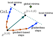
Figure 1: Server broadcasts $\boldsymbol{x}^{(t,0)}$ to clients for local training in round $t$. Clients perform extra gradientless updates, accelerating convergence of the aggregate model $\boldsymbol{x}^{(t+1,0)}$.

When clients train for $\tau_{i}$ local steps, they accumulate local momentum which contains useful information relevant to the next update. GeL exploits this local momentum to perform the guesses. More precisely, clients in GeL take additional steps in the direction of the accumulated momentum (guessed updates). Our generic guessing procedure features two advantages. First, it can be flexibly applied on top of several FL algorithms, including FedProx (Li et al. 2020b), FedNova (Wang et al. 2020) and FedYogi (Reddi et al. 2021). Such combinations leverage GeL (for fast empirical convergence) while tackling specific problems (, client-drift using FedProx) in the face of constrained computational and network budgets. Second, it relieves the need for exhaustive tuning of learning rates.

The guessing procedure significantly improves the performance of bad learning rate parameters, which otherwise would achieve deteriorated test performance. A crucial component of any ML training pipeline is hyperparameter optimization (HPO) (Lavesson and Davidsson 2006; Mantovani et al. 2015; Probst, Bischl, and Boulesteix 2018; Weerts, Mueller, and Vanschoren 2020), particularly learning rate (Keskar et al. 2017; Nar and Sastry 2018; Wu, Ma, and E 2018; Charles and Konečný 2020). However, when training on decentralized data, this tuning of hyperparameters is notoriously expensive and time-consuming (Kairouz et al. 2020). Adaptive optimizers like FedYogi (Reddi et al. 2021) increase the range of well-performing parameter values but still require grid inspection of different client and server learning rates $(\eta_{l},\eta)$. Our empirical results show that the FedYogi + GeL combination improves the test performance across a large set of values in this grid, thus significantly relieving the need for exhaustive tuning of learning rates.

Contributions

• We introduce GeL, a novel algorithm that compensates for limitations of constrained devices and varying system capabilities in FL by enabling guessed model updates for free ($\S$3.1).

• Based on the general theoretical framework of Wang  (2020), we provide a convergence analysis along with insights about the guessing in GeL ($\S\S$ 3.2 and 3.3).

• We conduct extensive experiments on three different learning tasks and demonstrate that GeL converges up to 30% faster in the number of communication rounds than the FedAvg baseline with client momentum ($\S$4.2).

• We show that GeL can be flexibly combined with state-of-the-art FL algorithms (FedProx, FedNova and FedYogi) while boosting their empirical performance by up to 40% ($\S\S$ 4.3 and 4.5).

• We demonstrate the benefits of GeL in improving test performance across a range of learning rate values. Our results show that using GeL eases tuning while achieving fast empirical convergence ($\S\S$ 4.4 and 4.5).

2 Related work and background

Computation heterogeneity in FL.

Heterogeneity in Federated Learning has received wide attention  (Bonawitz et al. 2019; Kairouz et al. 2020; Li et al. 2020a; Wang et al. 2021). FedAvg (McMahan et al. 2017) is the standard algorithm for federated training, though it was not particularly designed to address heterogeneity. FedProx (Li et al. 2020b) introduces a proximal penalty to keep client models close to the server model. In the presence of varying compute budgets, Wang  (2020) show that federated optimization algorithms can converge to an inconsistent objective function. To tackle this, FedNova aggregates normalized gradients to ensure consistency. Other approaches, such as HeteroFL (Diao, Ding, and Tarokh 2021) and AdaptCL (Zhou et al. 2021), allow clients to have heterogeneous models, enabling slower clients to train on smaller architectures and meet reporting deadlines. On similar lines, AQFL (Abdelmoniem and Canini 2021) adapts quantization levels on client devices to address heterogeneity. While these approaches are orthogonal, GeL differs in not only attenuating the impact of heterogeneity but also relieving the need for exhaustive learning rate tuning as we discuss next.

Hyperparameter tuning in FL.

HP selection in FL is a challenging problem (Zhou et al. 2023; Khodak et al. 2021). FedEx (Khodak et al. 2021) enhances tuning algorithms (Bergstra and Bengio 2012; Li et al. 2017) by using the weight-sharing technique of Neural Architecture Search (NAS), but still requires search-based techniques for certain global HPs. FLoRA (Zhou et al. 2023) achieves one-shot HPO in FL by aggregating loss surfaces from clients, yet at considerable client-side overheads.

Learning rate is a crucial HP (Nar and Sastry 2018; Charles and Konečný 2020). Adaptive optimizers like Adam (Kingma and Ba 2017) and Yogi (Zaheer et al. 2018) are less sensitive to learning rate tuning, thus representing robust alternatives to algorithms based on stochastic gradient descent (SGD). The FedOpt framework (Reddi et al. 2021) proposes FL equivalents of adaptive optimizers and studies their sensitivity to client ($\eta_{l}$) and server learning rates ($\eta$).

Thereby, an algorithm is considered as easy to tune if it produces good performance across several choices of parameter values (Reddi et al. 2021). We analyze GeL in the FedOpt framework and demonstrate improved performance across various $(\eta_{l},\eta)$ combinations for FedAvg and FedYogi, thus reducing the need for exhaustive tuning. Moreover, combining FedYogi with GeL produces significantly faster empirical convergence, as we show in $\S$4.5.

Utility of momentum.

Although vanilla SGD provides reasonable performance, the robust and fast convergence of momentum-based optimizers has been critical to the success of deep learning applications (Sutskever et al. 2013; Cutkosky and Orabona 2019). In the context of FL, Wang  (2020) report that using SGD with momentum (SGDM) as the client-side optimizer (ClientOpt) can effectively improve performance. We refer to the version of the FedAvg algorithm that uses SGDM as the ClientOpt as FedAvgCM. To illustrate the performance difference when using momentum, we experiment and chart in Figure 2 the learning curves for three different tasks using FedAvg and FedAvgCM algorithms. Notably, using momentum speeds up convergence with respect to the vanilla version by nearly $2\times$ in communication rounds. In this work, we exploit momentum to achieve client-side guessing in the face of limited computational budgets, as described next.

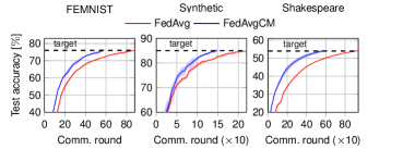
Figure 2: Using client-side momentum achieves target accuracy nearly 2$\times$ faster in communication rounds.

Notation.

$\boldsymbol{x}_{i}^{(t,k)}$ refers to the model parameters in round $t$ after $k$ local steps of training at client $i$. $\boldsymbol{g}_{i}^{(t,k)}$ is the stochastic gradient of the loss function computed using $\boldsymbol{x}_{i}^{(t,k)}$ on a mini-batch of data. $\boldsymbol{x}^{(t,0)}$ (without subscript $i$ and $k=0$) refers to the server model in round $t$.

3 GeL

Recall that, in FL, participating clients are often limited in their capacity to contribute to the training process. We refer to this limitation by their computational budget $\tau_{i}$, which dictates the number of model update steps that the client performs when participating in a training round. Given the computational budget constraints of clients $[\tau_{1},\tau_{2},\ldots,\tau_{C}]$ selected for a training round, the goal of GeL is to maximize the amount of progress made towards the optimal global model.

3.1 GeL: Guess and Learn Algorithm

GeL achieves its goal by guessing future model update steps for every client. The number of such updates is given by $[\tau^{\prime}_{1},\tau^{\prime}_{2},\ldots,\tau^{\prime}_{C}]$. Therefore, each client virtually performs $[\tau_{1}+\tau^{\prime}_{1},\tau_{2}+\tau^{\prime}_{2},\ldots,\tau_{C}+\tau^{\prime}_{C}]$ total learning steps, thereby boosting convergence. These guessed updates do not require any extra gradient computation but only a model update step, a much faster computation than a forward plus a backward pass through the deep model.

In order to perform the guessing, GeL leverages optimizers that accumulate a running first moment of gradients on the client side. In this work, we present our analysis and results using the SGDM (SGD with momentum) as the ClientOpt, although other choices like Adam and Yogi are also possible. On the server side, one is free to choose any server-side optimizer (ServerOpt). Therefore, GeL can be flexibly combined with several federated algorithms, including FedProx and FedNova. Table 3 (Appendix A) provides a complete list of all algorithms and their corresponding GeL versions along with the client and server optimizers used by each. We detail next the procedure for guessed steps.

The SGDM optimizer maintains a running moment of gradients, also known as velocity ($\boldsymbol{v}$), as follows:

$$\boldsymbol{v}_{i}^{(t,k+1)}=\alpha\boldsymbol{v}_{i}^{(t,k)}-\eta_{l}\boldsymbol{g}_{i}^{(t,k)}$$ (1)

where $\alpha$ is the momentum decay factor and $\eta_{l}$ is the client learning rate. The weights of the model are then updated using the current momentum instead of the current gradient:

$$\boldsymbol{x}_{i}^{(t,k+1)}=\boldsymbol{x}_{i}^{(t,k)}+\boldsymbol{v}_{i}^{(t,k+1)}$$ (2)

Upon training for $\tau_{i}$ local steps, clients produce $\boldsymbol{x}_{i}^{(t,\tau_{i})}$ as the final local model. At this point, the clients have exhausted their computational budgets $\tau_{i}$ and no more gradients can be computed. Notably, the accumulated momentum $\boldsymbol{v}_{i}^{(t,\tau_{i})}$ still contains useful information for the next update. In the absence of the next gradient, the value of the gradient can be substituted with a proxy.

$$\boldsymbol{v}_{i}^{(t,\tau_{i}+1)}=\alpha\boldsymbol{v}_{i}^{(t,\tau_{i})}-\eta_{l}\boldsymbol{g}_{i}^{(proxy)}$$ (3)

In GeL, we use $\boldsymbol{g}_{i}^{(proxy)}=0$. This can be interpreted as deriving the subsequent update steps solely from the accumulated momentum. Repeating this for $k$ steps, we have

$$\boldsymbol{v}_{i}^{(t,\tau_{i}+k)}=\alpha\boldsymbol{v}_{i}^{(t,\tau_{i}+k-1)}\ldots=\alpha^{k}\boldsymbol{v}_{i}^{(t,\tau_{i})}$$ (4)

Consequently, the model will be updated as follows:

$$\boldsymbol{x}_{i}^{(t,\tau_{i}+\tau^{\prime}_{i})} =\boldsymbol{x}_{i}^{(t,\tau_{i})}+\sum_{k=1}^{\tau^{\prime}_{i}}\boldsymbol{v}_{i}^{(t,\tau_{i}+k)}\text{ \hskip 22.76219pt (from eqn.~{}\ref{eqn:mom_model_update_on_clients})}$$

$$=\boldsymbol{x}_{i}^{(t,\tau_{i})}+\left(\sum_{k=1}^{\tau^{\prime}_{i}}\alpha^{k}\right)\boldsymbol{v}_{i}^{(t,\tau_{i})}\text{\hskip 5.69054pt (from eqn.~{}\ref{eqn:recurrence_v})}$$

The final model after $\tau^{\prime}_{i}$ guessed steps is:

$$\boldsymbol{x}_{i}^{(t,\tau_{i}+\tau^{\prime}_{i})}=\underbrace{\boldsymbol{x}_{i}^{(t,\tau_{i})}}_{\begin{subarray}{c}\text{Last model before the}\\ \text{budget is exhausted}\end{subarray}}+\underbrace{\left(\alpha\frac{1-\alpha^{\tau^{\prime}_{i}}}{1-\alpha}\right)\boldsymbol{v}_{i}^{(t,\tau_{i})}}_{\begin{subarray}{c}\text{Nudge in the direction}\\ \text{ of momentum.}\end{subarray}}\\$$ (5)

The guessed learning steps are effectively a nudge in the direction of momentum with the corresponding step size $\frac{\alpha(1-\alpha^{\tau^{\prime}_{i}})}{1-\alpha}$ decided by the number of guessed steps $\tau^{\prime}_{i}$. More importantly, the number of guessed updates $\tau^{\prime}_{i}$ can be chosen differently for different clients, possibly depending on their actual work $\tau_{i}$. Recall from $\S$1 that the server requests a fixed number of learning steps $\tau$ in the stipulated time window. One approach to establishing $\tau^{\prime}_{i}$ is to assign it the value of the remaining work, $\tau^{\prime}_{i}=\tau-\tau_{i}$. This strategy also homogenizes the total virtual work $\tau_{i}+\tau^{\prime}_{i}$ across the clients. We demonstrate the results with this strategy in $\S$4. The pseudocode for GeL is presented in Algorithm algo:GeL (Appendix B).

3.2 Convergence analysis of GeL

We now present the convergence result for the FedAvgCM + GeL algorithm. This result is based on the general theoretical framework of Wang , (2020) which subsumes a suite of FL algorithms whose accumulated local changes $(\boldsymbol{x}_{i}^{(t,\tau_{i})}-\boldsymbol{x}_{i}^{(t,0)})$ can be written as a linear combination of gradients. More precisely, algorithms for which

$$\Delta_{i}^{(t)}=\boldsymbol{x}_{i}^{(t,\tau_{i})}-\boldsymbol{x}_{i}^{(t,0)}=-\eta_{l}\boldsymbol{G}_{i}^{(t)}\boldsymbol{a}_{i}$$

where matrix $\boldsymbol{G}_{i}^{(t)}=[\boldsymbol{g}_{i}^{(t,0)},\boldsymbol{g}_{i}^{(t,1)},\ldots,\boldsymbol{g}_{i}^{(t,\tau_{i-1})}]\in\mathbb{R}^{d\times\tau_{i}}$ stacks all local gradients and $\boldsymbol{a}_{i}\in\mathbb{R}^{\tau_{i}}$ defines the coefficients of this linear combination are subsumed by the general theoretical framework.

Since the guessed step is derived solely out of the first moment of gradients (a linear combination), the accumulated updates in FedAvgCM + GeL algorithm obey the above structure. We derive the accumulated update and the gradient coefficient vector $\boldsymbol{a}_{i}$ in an elaborate proof in Appendix C.3, leading to:

$$\boldsymbol{x}_{i}^{(t,\tau_{i}+\tau^{\prime}_{i})}-\boldsymbol{x}_{i}^{(t,0)}=-\eta_{l}\sum_{k=0}^{\tau_{i}-1}\left[\frac{1-\alpha^{\tau^{\prime}_{i}+\tau_{i}-k}}{1-\alpha}\right]\boldsymbol{g}_{i}^{(t,k)}$$

Lemma 1 (Accumulated updates in FedAvgCM + GeL).

When performing $\tau_{i}$ gradient steps and $\tau^{\prime}_{i}$ guessed steps, the accumulated updates in the FedAvgCM + GeL algorithm form a linear combination of gradients with the gradient coefficients, given by

$$\boldsymbol{a}_{i}=[1-\alpha^{\tau^{\prime}_{i}+\tau_{i}},1-\alpha^{\tau^{\prime}_{i}+\tau_{i}-1},...,1-\alpha^{\tau^{\prime}_{i}+1}]/(1-\alpha)$$ (6)

Based on Lemma 1 and the above theoretical framework, we show that FedAvgCM + GeL algorithm converges at the rate $\mathcal{O}(1/\sqrt{m\bar{\tau}T})$, where $\bar{\tau}=\frac{1}{m}\sum_{i=1}^{m}\tau_{i}$ and $T$ is the number of communication rounds (proof in Appendix C).

3.3 Discussion and insights

The presented analysis serves two purposes: (i) it confirms that the guessed updates in GeL do not jeopardize the convergence by showing that FedAvgCM + GeL has a similar asymptotic convergence rate to standard FedAvg, with slightly different constants in the inequality; and (ii) it provides interesting insights into understanding GeL.

Guesses in GeL are derived out of gradients computed until the budget $\tau_{i}$ and accumulated in the momentum vector. We showed that the final update in GeL forms a linear combination of gradients with the coefficients described in eqn. 6. We contrast these with the coefficients for two instances of the FedAvgCM algorithm (, no GeL), one performing $\tau_{i}$ gradient-based steps, and the other $\tau_{i}+\tau^{\prime}_{i}$ gradient-based steps in Figure 3.

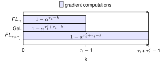
Figure 3: Gradient coefficients of different algorithms (only numerators shown, the denominator is $1-\alpha$ for all).

Interestingly, the coefficients in GeL correspond exactly to the coefficients that would have resulted for all gradients $\boldsymbol{g}_{i}^{(t,k)}$ with $k\leq\tau_{i}-1$, had the client performed all $\tau_{i}+\tau^{\prime}_{i}$ steps as actual gradient-based steps. In essence, GeL computes the sequential inter-dependent gradients in a regular way. However, once computed, it cleverly combines them using coefficients that would have resulted if a greater number of actual gradients were computed. This simple modification results in notable speedups, as we demonstrate in $\S$4.

We note that in GeL no momentum state is transferred between the server and the clients or vice-versa. Hence, GeL does not incur additional communication overhead. Clients remain stateless and reset their momentum to zero when commencing the training for the current round. Consequently, the accumulated momentum is local to the current training round for every client. Finally, GeL is also compatible with model compression (Wang et al. 2018; Sattler et al. 2020; Li et al. 2020c), differential privacy (Wei et al. 2020) and secure aggregation (Bonawitz et al. 2016; So, Güler, and Avestimehr 2021).

4 Experimental results

We present our experimental setup in $\S$4.1. Section 4.2 compares GeL to the FedAvgCM baseline, while $\S\S$ 4.3 and 4.5 evaluate GeL combined with different algorithms. The performance of GeL under untuned learning rate settings is studied in $\S\S$ 4.4 and 4.5.

4.1 Experimental setup

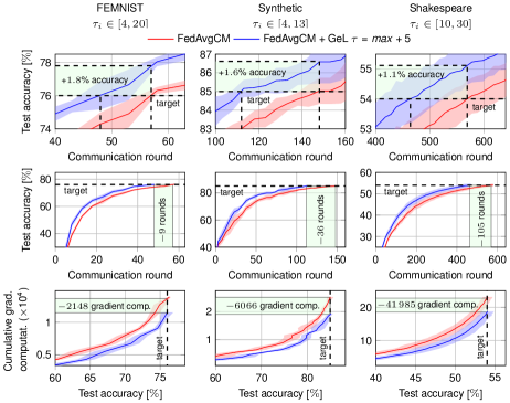
Figure 4: GeL performance compared to FedAvgCM across datasets. GeL achieves target accuracy faster than FedAvgCM (row-2), and superior accuracy when FedAvgCM reaches target (row-1). Needing fewer communication rounds, GeL significantly reduces gradient computations compared to FedAvgCM (row-3).

Datasets And Models We evaluate all algorithms on three different learning tasks – image classification on the FEMNIST dataset, text generation on the Shakespeare dataset, and cluster identification on the Synthetic dataset. These datasets are taken from the LEAF benchmark (Caldas et al. 2019) for FL, used in several previous works (McMahan et al. 2017; Li et al. 2020b; Reddi et al. 2021; Charles et al. 2021). The datasets also exhibit a natural non-IID partitioning, each writer is a separate client in the FEMNIST dataset. We use the same models as McMahan  (2017) and Li  (2020b) in our experiments for all 3 learning tasks. Table 4 (Appendix D) summarizes the learning tasks, datasets, and models.

Hyperparameters

We tune the client learning rate $(\eta_{l})$ for the FedAvgCM baseline. FedProx, FedNova, and GeL use the same tuned learning rate for fairness. The FedAvg algorithm in Figure 2 has a separately tuned client learning rate due to the absence of client momentum. Default server learning rate $\eta=1$ is used in all experiments except for the FedOpt framework ($\S$4.5), where we tune both the client and server learning rates $(\eta_{l},\eta)$. The number of selected clients $(C)$ per round is fixed at 20. Batch sizes of 5, 20, and 20 are used for the Synthetic, FEMNIST, and Shakespeare datasets, respectively. We set the momentum parameter ($\alpha$) to 0.9 and use $\beta_{1}=0.9$ and $\beta_{2}=0.99$ for the Yogi optimizer. The adaptivity parameter of the Yogi optimizer is fixed at $10^{-3}$. More details on hyperparameter tuning are in Appendix E.

Client budgets

Following Li  (2020b), we perform the budget assignment every round in two steps: (1) clients are selected uniformly at random; and (2) each selected client uniformly randomly samples budgets from a range $\tau_{i}\in[a,b]$. This resembles realistic FL settings where client budgets are not only heterogeneous but may also vary across rounds for any individual client. We set the server’s expected $\tau$ to $b+5$. This means that the server expects each client to perform $b+5$ local update steps. The budget ranges ($\tau_{i}$) along with the desired value of $\tau$ are stated on top of the charts (Figure 4) per dataset. All our experiments use these budgetary constraints.

Metrics

We evaluate the performance of GeL along four metrics: top-1 test accuracy, speedup, network savings, and the number of gradient computations. The performance speedup is measured in rounds of communication to achieve a predefined target accuracy. We set these accuracy targets similar to the ones used in previous works  (McMahan et al. 2017; Caldas et al. 2019; Abdelmoniem and Canini 2021). The network savings, presented alongside speedups, highlight the reduced communication costs. Finally, we measure the evolution of test accuracy against the cumulative number of gradients computed by all participating clients until the target accuracy has been reached. This metric specifically showcases the role of GeL in maximizing progress under stringent computational budget constraints. We run each experiment with 5 random seeds and present the average values and the 95% confidence interval.

We will provide an open-source implementation of GeL for reusability and reproducibility.

4.2 GeL against FedAvgCM

Dataset	Target	$\eta_{l}$		Comm. rounds until target accuracy		Speed up	# Model	Network
	accuracy			FedAvgCM	GeL		parameters	savings
FEMNIST	76%	$0.02$	tuned	57	48	18.8%	$6.1\text{\times}{10}^{5}$	$1.08\text{\,}\mathrm{GiB}\text{/}$
		$0.01$	untuned	95	69	37.7%		$3.11\text{\,}\mathrm{GiB}\text{/}$
Synthetic	85%	$0.01$	tuned	148	112	32.1%	$305$	$0.58\text{\,}\mathrm{MiB}\text{/}$
		$0.005$	untuned	176	135	30.4%		$0.66\text{\,}\mathrm{MiB}\text{/}$
Shakespeare	54%	$0.3$	tuned	569	464	22.6%	$8.2\text{\times}{10}^{5}$	$3.73\text{\,}\mathrm{GiB}\text{/}$
		$0.15$	untuned	820	639	28.3%		$6.44\text{\,}\mathrm{GiB}\text{/}$

Table 1: Performance comparison of GeL to FedAvgCM. GeL reaches the target accuracy up to 20-38% faster in communication rounds in both tuned and untuned scenarios. In addition, we report the economy of resources in GeL in terms of network savings.

Recall from Section 2 that momentum enables significant speedup for all the learning tasks. Consequently, we consider the FedAvgCM algorithm as the baseline instead of the standard FedAvg algorithm throughout our experiments. We refer to the application of GeL on FedAvgCM as FedAvgCM + GeL (Table 3, Appendix A). Figure 4 presents the performance results, with rows 1 and 2 showing the test accuracy versus communication rounds, and row 3 illustrating the evolution of test accuracy with respect to total gradients computed by the system.

As described in $\S$3, GeL performs $\tau^{\prime}_{i}=\tau-\tau_{i}$ guessed updates for every client. By just performing these free learning steps, GeL speeds up convergence to target accuracy by up to 30% in rounds of communication (speedup column of Table 1). Notably, even for the challenging Shakespeare dataset, GeL requires over 100 fewer rounds to converge. Furthermore, when both GeL and FedAvgCM reach the target accuracy, GeL achieves higher accuracy in all learning tasks, with a notable increase of approximately 2% for the FEMNIST dataset (row-1 of Figure 4). In terms of computation, GeL consistently requires significantly fewer gradient computations compared to FedAvgCM to achieve equal accuracy across all learning tasks. This translates to thousands of saved computations, reaching up to $42\,000$ for the Shakespeare dataset (row-3 of Figure 4).

We also demonstrate that GeL is not very sensitive to large values of $\tau^{\prime}_{i}$ by setting $\tau^{\prime}_{i}=\infty$ in Section F.1. Additionally, we assess GeL under different budget ranges in Section F.2.

4.3 GeL applied to FedProx and FedNova

The FedProx and FedNova algorithms were designed to address compute heterogeneity (Section 2). We investigate their combination with GeL and examine whether GeL can accelerate their convergence.

Datasets	FedProx				FedNova
	Comm. rounds until		Speedup	GeL	Comm. rounds until		Speedup	GeL
	target accuracy			accuracy	target accuracy			accuracy
	Default	Default		beyond	Default	Default		beyond
		+ GeL		target [%]		+ GeL		target [%]
FEMNIST $\tau_{i}\in[4,20]$	49	38	28.9%	+2.19	63	55	11.5%	+1.04
Synthetic $\tau_{i}\in[4,13]$	157	112	40.2%	+1.18	118	103	14.6%	+0.94
Shakespeare $\tau_{i}\in[10,30]$	605	478	26.6%	+1.26	578	478	20.9%	+1.17

Table 2: GeL enhances existing FL algorithms by achieving earlier target accuracy (Speedup) and surpassing their accuracy (GeL accuracy beyond target) when measured at the round when the baseline (FedProx or FedNova) achieves the target.

FedProx + GeL

The gradients in the FedProx algorithm account for the proximal term along with the regular loss function. This being the only difference to FedAvgCM, guessed updates in GeL (eq. 5) can be directly applied on top of FedProx algorithm. Table 2 summarizes the results under the column FedProx. FedProx + GeL takes significantly fewer communication rounds to reach the same target accuracy as FedProx, achieving between 26 and 40% speedup across the learning tasks. In addition, FedProx + GeL reaches up to 2.19% higher test accuracy by the round when default FedProx achieves target accuracy. These findings show that GeL can be seamlessly combined with FedProx to boost the convergence of the latter.

FedNova + GeL

Similar to FedProx, GeL can also be easily applied on top of the FedNova algorithm (Wang et al. 2020). Table 2 summarizes the results under column FedNova. With a simple modification resulting from guessed updates, GeL boosts default FedNova by 10-20%. Moreover, it reaches nearly 1% higher target accuracy for all datasets by the round when default FedNova reaches the target accuracy. We also observe that the results of default FedNova are not significantly different from baseline FedAvgCM in Table 1. We speculate a modest objective inconsistency (which FedNova is designed to resolve) observed in practice as a reason for this behavior. However, the results still indicate that GeL can be beneficially combined with FedNova to speed up convergence.

4.4 GeL in untuned learning rate settings

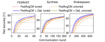
Figure 5: Impact of GeL on performance with tuned and untuned learning rate ($\eta_{l}$). GeL boosts convergence even when using a sub-optimal learning rate.

As motivated in $\S\S$ 1 and 2, tuning learning rates is an arduous task in FL. Interestingly, GeL presents an alternative to exact tuning: gradients can be computed using untuned learning rates, but combined using coefficients that maximize progress. In $\S$4.5, we present the final test performance after very long executions of the algorithms and show the effectiveness of GeL in improving poor test performance of bad parameter values. In this section, we focus on the speedup achieved by GeL when comparing two sets of learning rate values: the best and a non-best learning rate that still achieves the target accuracy. We set the non-best learning rate to a value equal to half of the best one, although in practice this could be arbitrary.

Figure 5 and Table 1 demonstrate the results. In the untuned setting, GeL converges nearly 38% faster for the FEMNIST dataset. For the Synthetic dataset, GeL converges in even fewer rounds than the tuned FedAvgCM baseline. Finally, for the challenging Shakespeare dataset, the speedup rises to 28% in the untuned case from 22% in the tuned case, taking over 150 fewer communication rounds to reach the same accuracy.

Intuitively, GeL exhibits this behavior because lower learning rates provide more room for improvement through guessing. In other words, when step sizes are small, learning can smoothly progress in the direction of momentum, which GeL precisely exploits. Furthermore, the amplified speed-up leads to nearly double network savings in data volume compared to the tuned case (for FEMNIST and Shakespeare datasets), as indicated in Table 1. These results demonstrate that GeL achieves significant performance boosts without requiring perfectly tuned learning rates, making it a cost-effective alternative to expensive tuning.

4.5 GeL in FedOpt framework

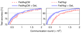
Figure 6: FedOpt framework. GeL enhances the empirical convergence of both FedAvgCM and FedYogi.

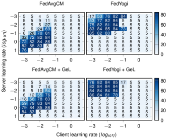
Figure 7: Test accuracy grid for the FEMNIST dataset. GeL enhances performance for many parameter values, relieving exhaustive tuning. While it also impacts a few combinations, these are on the extreme and arguably not the safest.

In this section, we analyze the impact of server-side optimization on GeL performance. We evaluate FedAvgCM and FedYogi algorithms on the FEMNIST dataset with tuned client ($\eta_{l}$) and server learning ($\eta$) rates, following the procedure outlined in (Reddi et al. 2021). See Appendix E for more details on tuning. We observe in Figure 6 that the guessing mechanism in GeL continues to expedite empirical convergence, leading to higher accuracy within a fixed number of communication rounds. Furthermore, algorithms in the FedOpt framework achieve better accuracies than previously, emphasizing the benefits of tuning both client and server learning rates. This however comes at a significant cost of tuning.

As previously established, we deem an algorithm as easy to tune in case it produces good performance across several choices of parameter values. GeL, in particular, through guessing updates can restore the performance of bad parameter values. To justify this, we chart in Figure 7 the test accuracy grids upon running 1000 rounds of training on the FEMNIST dataset. Note that GeL improves the test performance for many $(\eta_{l},\eta)$ values, providing good performance over a large set. This is especially evident for the FedYogi + GeL combination. While it hurts the performance of a few parameters, we argue that these parameters are the ones with very high learning rate values. Hence, they are not the safest choice as they are susceptible to overshooting and divergence. In conclusion, GeL alleviates the strong need for exhaustive tuning, serving as a practical alternative.

5 Conclusion

We designed GeL, our guess and learn algorithm that addresses slow convergence in challenging heterogeneous FL settings. The novelty of GeL lies in its gradient-free guessing, thus speeding up convergence at no cost, while compensating for low-budget clients. We demonstrated the wide applicability of GeL by successfully implementing it on top of several state-of-the-art algorithms. In one of the most promising findings of the paper, we highlighted the utility of GeL as a practical alternative to exhaustive tuning. Future research directions include exploring the applicability of GeL in other FL setups, asynchronous FL (Huba et al. 2022) for controlling the staleness of updates.

Organization of the Appendix

Appendix A presents an exhaustive list of algorithms considered in this work, their GeL versions along with their respective client and server optimizers. Appendix B provides the pseudocode of GeL. In Appendix C, we present the complete convergence result of FedAvgCM + GeL including the proof of Lemma 1. Appendix D provides additional details on the learning tasks while Appendix E elaborates on the hyperparameter tuning. Lastly, in Appendix F, we present additional results and discussion assessing the impact of (i) a large number of guessed updates, and (ii) varying client budget distributions $(\tau_{i})$.

Appendix A Algorithm List

We present the list of algorithms considered in this work along with their GeL versions in Table 3.

Algorithm	ClientOpt ($\eta_{l}$)		ServerOpt ($\eta$)
	Default	Algorithm + GeL
FedAvg (McMahan et al. 2017)	SGD	SGDM with guessed updates	SGD
FedAvgCM (Reddi et al. 2021)	SGDM	SGDM with guessed updates	SGD
FedProx (Li et al. 2020b)	Proximal SGDM	Proximal SGDM with guessed updates	SGD
FedNova (Wang et al. 2020)	SGDM	SGDM with guessed updates	SGD
FedYogi (Reddi et al. 2021)	SGD	SGDM with guessed updates	Yogi

Table 3: List of algorithms referred in this paper and their GeL versions. Vanilla SGD is referred as just SGD while SGDM stands for the SGD with momentum optimizer. We adopt the acronym name FedAvgCM. Further, we consider the version of FedNova with the above client and server optimizers due to its superior performance while it can use any client optimizer (Wang et al. 2020).

Appendix B Pseudocode of GeL

We provide the pseudocode of GeL in Algorithm 1 and describe it below. Similar to FedAvg, the server then selects a subset of clients and broadcasts the global model $\boldsymbol{x}^{(t,0)}$ along with the desired number of local steps $\tau$ for training in the current round (lines 4-7). After initialization (lines 12-13), the clients train on their local data only up to their computational budget $\tau_{i}$ instead of $\tau$ (lines 14-18). For the remaining undone steps $\tau-\tau_{i}$, the clients compensate by performing an equivalent number of guessed update steps $\tau^{\prime}_{i}$ (lines 19-20). Note that this is computed as a single operation (line 20) instead of iterative steps. It also does not entail any gradient computations, hence is a relatively cheap operation. Finally, the server aggregates received model updates (line 8) and produces the new global model using a ServerOpt of its choice (line 9).

1 Server Executes:

2 Initialise $\boldsymbol{x}^{(0,0)}$

3 for $t=0,1,2,\dots$ do

4      $S^{(t)}\leftarrow$ Server randomly selects $C$ clients

5      for each $i\in S^{(t)}$ in parallel do

6           $\Delta_{i}^{(t)}=$ ClientUpdate$\left(i,\boldsymbol{x}^{(t,0)},\tau\right)$

7          

8           end for

9          $\Delta^{(t)}=\sum_{i\in S^{(t)}}p_{i}\Delta_{i}^{(t)}$

10           $\boldsymbol{x}^{(t+1,0)}=\text{\acs{ServerOpt}}(\boldsymbol{x}^{(t,0)},-\Delta^{(t)},\eta,t)$

11          

12           end for

          ClientUpdate($i,\boldsymbol{x}^{(t,0)},\tau$):

            $\vartriangleright$ Client $i$

           $\boldsymbol{v}_{i}^{(t,0)}=0$

            $\vartriangleright$ initialize momentum

           $\boldsymbol{x}_{i}^{(t,0)}=\boldsymbol{x}^{(t,0)}$

            $\vartriangleright$ initialize model

           $\vartriangleright$ Compute up to budget $\tau_{i}$

13           for step $k=1$ to $\tau_{i}$ do

14                Compute $\boldsymbol{g}_{i}^{(t,k-1)}$

15                $\boldsymbol{v}_{i}^{(t,k)}=\alpha\boldsymbol{v}_{i}^{(t,k-1)}-\eta_{l}\boldsymbol{g}_{i}^{(t,k-1)}$

16                $\boldsymbol{x}_{i}^{(t,k)}=\boldsymbol{x}_{i}^{(t,k-1)}+\boldsymbol{v}_{i}^{(t,k)}$

17               

18                end for

               

                $\vartriangleright$ Guessed update step

19                Choose $\tau^{\prime}_{i}=\tau-\tau^{\prime}_{i}$ or simply use $\tau^{\prime}_{i}=\infty$

20                $\boldsymbol{x}_{i}^{(t,\tau_{i}+\tau^{\prime}_{i})}=\boldsymbol{x}_{i}^{(t,\tau_{i})}+\alpha\frac{1-\alpha^{\tau^{\prime}_{i}}}{1-\alpha}\boldsymbol{v}_{i}^{(t,\tau_{i})}$

21                $\Delta_{i}^{(t)}=\boldsymbol{x}_{i}^{(t,\tau_{i}+\tau^{\prime}_{i})}-\boldsymbol{x}_{i}^{(t,0)}$

22                return $\Delta_{i}^{(t)}$ to the server

Algorithm 1 GeL. The $C$ clients are indexed by $i$; $\tau$ is the number of steps expected by the server; $\tau_{i}$ and $\tau^{\prime}_{i}$ are the computational budget and number of guessed updates; $p_{i}$ is the weight; $\eta_{l}$ and $\eta$ refer to the client and the server learning rate respectively. The server can choose any ServerOpt while the client must use an optimizer that accumulates the first moment of gradients (SGDM shown below).

Appendix C Detailed convergence analysis for FedAvgCM + GeL algorithm

In this section, we detail the convergence result for the FedAvgCM + GeL algorithm presented in $\S$3.2. To begin, we first revisit the federated optimization setting.

C.1 The federated optimization setting

The goal of FL is to minimize the following objective function with a total of $m$ clients:

$$\min_{\boldsymbol{x}\in\mathbb{R}^{d}}\left[F(\boldsymbol{x}):=\sum_{i=1}^{m}p_{i}F_{i}(\boldsymbol{x})\right]$$ (7)

where $F_{i}(\boldsymbol{x})=\frac{1}{n_{i}}\sum_{\xi\in\mathcal{D}_{i}}f_{i}(\boldsymbol{x};\xi)$ is the local objective function on the $i^{th}$ client, $p_{i}=n_{i}/n$ denotes the relative sample size and $n=\sum_{i=1}^{m}n_{i}$. The function $f_{i}$ represents the loss function (possibly non-convex) on client $i$ defined by the learning model $\boldsymbol{x}$ and samples $\xi$ taken from the local dataset $\mathcal{D}_{i}$.

Learning occurs in repetitions of communication rounds where in the $t$-th communication round, the server selects a subset $S^{(t)}$of available clients and broadcasts the global model $\boldsymbol{x}^{(t,0)}$ for local training. Generally, the number of clients selected $|S^{(t)}|=C$ is kept fixed across communication rounds. Further, the server requests a fixed computation in a number of steps $\tau$ and waits a stipulated time window to receive updates from the selected clients (McMahan et al. 2017; Bonawitz et al. 2019). However, as described in Section 1, each client manages to perform only a portion of the requested computation, which we denote $\tau_{i}$. It corresponds to the computational budget of the $i$-th client, , the number of local learning steps that this client is able to perform in the stipulated time window. Thus, each client performs a different number of local steps $\{\tau_{i}\}_{i=1}^{C}$.

C.2 Heterogeneous federated optimization framework

Wang , (2020) proposed the general theoretical framework to analyze federated algorithms under heterogeneous client budgets. In this framework, FL algorithms can be expressed using a general rule as follows:

$$\boldsymbol{x}^{(t+1,0)}=\boldsymbol{x}^{(t,0)}-\tau_{\text{eff}}\sum_{i=1}^{m}w_{i}.\eta_{l}\boldsymbol{d}_{i}^{(t)}$$ (8)

which optimizes

$$\widetilde{F}(\boldsymbol{x})=\sum_{i=1}^{m}w_{i}F_{i}(\boldsymbol{x})$$ (9)

where $\boldsymbol{d}_{i}^{(t)}$ is the normalized gradient, $w_{i}$’s are aggregation weights and $\tau_{\text{eff}}$ is the effective step size. The normalized gradient is defined as

$$\boldsymbol{d}_{i}^{(t)}=\frac{\boldsymbol{G}_{i}^{(t)}\boldsymbol{a}_{i}}{||\boldsymbol{a}_{i}||_{1}}$$

where the matrix $\boldsymbol{G}_{i}^{(t)}=[\boldsymbol{g}_{i}^{(t,0)},\boldsymbol{g}_{i}^{(t,1)},\ldots,\boldsymbol{g}_{i}^{(t,\tau_{i-1})}]\in\mathbb{R}^{d\times\tau_{i}}$ stacks all local stochastic gradients, the vector $\boldsymbol{a}_{i}\in\mathbb{R}^{\tau_{i}}$ defines the coefficients of these gradients and $||\boldsymbol{a}_{i}||_{1}$ is the $\ell_{1}$ norm of the vector $\boldsymbol{a}_{i}$. Any FL algorithm whose accumulated local changes $\Delta_{i}^{(t)}=\boldsymbol{x}_{i}^{(t,\tau_{i})}-\boldsymbol{x}_{i}^{(t,0)}$ can be written as a linear combination of local gradients is subsumed by this formulation.

Previous FL algorithms can be shown to be special cases of this formulation obtained by substituting appropriate values of $w_{i}$, $\tau_{\text{eff}}$, and $\boldsymbol{a}_{i}$. Specifically, given the value of $\boldsymbol{a}_{i}$, Wang (2020) show that FL algorithms take on the following values for $w_{i}$ and $\tau_{\text{eff}}$,

$$w_{i}=\frac{p_{i}||\boldsymbol{a}_{i}||_{1}}{\sum_{i=1}^{m}p_{i}||\boldsymbol{a}_{i}||_{1}}$$

$$\tau_{\text{eff}}=\sum_{i=1}^{m}p_{i}||\boldsymbol{a}_{i}||_{1}.$$

Note that the specification of $\boldsymbol{a}_{i}$ defines all variables in the general update rule of equation 8.

C.3 Proof of Lemma 1: Accumulated updates in FedAvgCM + GeL algorithm

Now we prove that the update rule for the FedAvgCM + GeL algorithm forms a linear combination of gradients, allowing us to apply the above general theoretical framework. To begin, recall the SGD with momentum equation 1 and equation 2:

$$\begin{split}\boldsymbol{v}_{i}^{(t,k+1)}&=\alpha\boldsymbol{v}_{i}^{(t,k)}-\eta_{l}\boldsymbol{g}_{i}^{(t,k)}\\ \boldsymbol{x}_{i}^{(t,k+1)}&=\boldsymbol{x}_{i}^{(t,k)}+\boldsymbol{v}_{i}^{(t,k+1)}\end{split}$$

By a simple recursion, we get:

$$\begin{split}\boldsymbol{v}_{i}^{(t,k)}&=\alpha\boldsymbol{v}_{i}^{(t,k-1)}-\eta_{l}\boldsymbol{g}_{i}^{(t,k-1)}\\ &=-\eta_{l}\sum_{j=0}^{k-1}\alpha^{k-1-j}\boldsymbol{g}_{i}^{(t,j)}\hskip 14.22636pt(\text{where }\boldsymbol{v}_{i}^{(t,0)}=0)\end{split}$$

Hence:

$$\begin{split}\boldsymbol{x}_{i}^{(t,\tau_{i})}-\boldsymbol{x}_{i}^{(t,0)}&=\sum_{k=1}^{\tau_{i}}\boldsymbol{v}_{i}^{(t,k)}\\ &=-\eta_{l}\sum_{k=1}^{\tau_{i}}\sum_{j=0}^{k-1}\alpha^{k-1-j}\boldsymbol{g}_{i}^{(t,j)}\end{split}$$

Moreover, recall from equation 5 that:

$$\begin{split}\boldsymbol{x}_{i}^{(t,\tau_{i}+\tau^{\prime}_{i})}&-\boldsymbol{x}_{i}^{(t,\tau_{i})}=\left(\alpha\frac{1-\alpha^{\tau^{\prime}_{i}}}{1-\alpha}\right)\boldsymbol{v}_{i}^{(t,\tau_{i})}\\ &=-\eta_{l}\left(\alpha\frac{1-\alpha^{\tau^{\prime}_{i}}}{1-\alpha}\right)\sum_{j=0}^{\tau_{i}-1}\alpha^{\tau_{i}-1-j}\boldsymbol{g}_{i}^{(t,j)}\end{split}$$

By combining the two equations above, we have:

$$\begin{split}&\boldsymbol{x}_{i}^{(t,\tau_{i}+\tau^{\prime}_{i})}-\boldsymbol{x}_{i}^{(t,0)}=\\ &-\eta_{l}\left(\alpha\frac{1-\alpha^{\tau^{\prime}_{i}}}{1-\alpha}\right)\sum_{j=0}^{\tau_{i}-1}\alpha^{\tau_{i}-1-j}\boldsymbol{g}_{i}^{(t,j)}\\ &-\eta_{l}\sum_{k=1}^{\tau_{i}}\sum_{j=0}^{k-1}\alpha^{k-1-j}\boldsymbol{g}_{i}^{(t,j)}\end{split}$$

Rewriting the second term on the right-hand side:

$$\begin{split}&\boldsymbol{x}_{i}^{(t,\tau_{i}+\tau^{\prime}_{i})}-\boldsymbol{x}_{i}^{(t,0)}=\\ &-\eta_{l}\left(\alpha\frac{1-\alpha^{\tau^{\prime}_{i}}}{1-\alpha}\right)\sum_{j=0}^{\tau_{i}-1}\alpha^{\tau_{i}-1-j}\boldsymbol{g}_{i}^{(t,j)}\\ &-\eta_{l}\sum_{j=0}^{\tau_{i}-1}g_{i}^{(t,j)}\sum_{k=0}^{\tau_{i}-j-1}\alpha^{k}\end{split}$$

Putting the coefficients together:

$$\begin{split}&\boldsymbol{x}_{i}^{(t,\tau_{i}+\tau^{\prime}_{i})}-\boldsymbol{x}_{i}^{(t,0)}=\\ &-\eta_{l}\sum_{j=0}^{\tau_{i}-1}\left[\left(\alpha\frac{1-\alpha^{\tau^{\prime}_{i}}}{1-\alpha}\right)\alpha^{\tau_{i}-1-j}+\left(\sum_{k=0}^{\tau_{i}-j-1}\alpha^{k}\right)\right]\boldsymbol{g}_{i}^{(t,j)}\\ &=-\eta_{l}\sum_{j=0}^{\tau_{i}-1}\left[\left(\alpha\frac{1-\alpha^{\tau^{\prime}_{i}}}{1-\alpha}\right)\alpha^{\tau_{i}-1-j}+\frac{1-\alpha^{(\tau_{i}-j)}}{1-\alpha}\right]\boldsymbol{g}_{i}^{(t,j)}\\ &=-\eta_{l}\sum_{j=0}^{\tau_{i}-1}\left[\frac{\alpha^{\tau_{i}-j}-\alpha^{\tau^{\prime}_{i}+\tau_{i}-j}+1-\alpha^{\tau_{i}-j}}{1-\alpha}\right]\boldsymbol{g}_{i}^{(t,j)}\\ &=-\eta_{l}\sum_{j=0}^{\tau_{i}-1}\left[\frac{1-\alpha^{\tau^{\prime}_{i}+\tau_{i}-j}}{1-\alpha}\right]\boldsymbol{g}_{i}^{(t,j)}\end{split}$$

Thus, the update rule of FedAvgCM + GeL can be expressed as a linear combination of gradients where the coefficient of $\boldsymbol{g}_{i}^{(t,j)}$ is $\frac{1-\alpha^{\tau^{\prime}_{i}+\tau_{i}-j}}{1-\alpha}$. With this, we obtain the coefficient vector $\boldsymbol{a}_{i}$:

$$\boldsymbol{a}_{i}=[1-\alpha^{\tau^{\prime}_{i}+\tau_{i}},1-\alpha^{\tau^{\prime}_{i}+\tau_{i}-1},...,1-\alpha^{\tau^{\prime}_{i}+1}]/(1-\alpha)$$ (10)

This proves our Lemma 1 presented in Section 3.2. Thus, FedAvgCM + GeL can also be expressed using the update rule Equation 8 which leads us to the following result.

C.4 Final convergence result

(Wang et al. 2020) show that for FL algorithms whose update rule follows Equation 8, thus subsuming FedAvgCM + GeL, the following convergence result holds under standard assumptions in the federated optimization literature (Bottou, Curtis, and Nocedal 2018; Wang et al. 2020; Karimireddy et al. 2021).

Assumption 1 (Smoothness).

$||\nabla F_{i}(\boldsymbol{x})-\nabla F_{i}(\hat{y})||\leq L||\boldsymbol{x}-\hat{y}||,\forall i\in\{1,2,\ldots,m\}$.

Assumption 2 (Unbiased gradients and bounded variance).

$\mathbb{E}_{\xi}[g_{i}(\boldsymbol{x}|\xi)]=\nabla F_{i}(\boldsymbol{x})$ and $\mathbb{E}_{\xi}[||g_{i}(\boldsymbol{x}|\xi)-\nabla F_{i}(\boldsymbol{x})||^{2}]\leq\sigma^{2},\forall i\in\{1,2,\ldots,m\},\sigma^{2}\geq 0$

Assumption 3 (Bounded Dissimilarity).

For any set of weights $\{w_{i}\geq 0\}_{i=1}^{m},\sum_{i=1}^{m}w_{i}=1$, there exist constants $\beta^{2}\geq 1,\kappa^{2}\geq 0$ such that $\sum_{i=1}^{m}w_{i}||\nabla F_{i}(\boldsymbol{x})||^{2}\leq\beta^{2}||\sum_{i=1}^{m}w_{i}\nabla F_{i}(\boldsymbol{x})||^{2}+\kappa^{2}$

Theorem 2 (Convergence to the $\widetilde{F}(\boldsymbol{x})$’s Stationary Point).

Under Assumptions 1 to 3, any federated optimization algorithm that follows the update rule (8), will converge to a stationary point of a surrogate objective $\smash{\widetilde{F}}(\boldsymbol{x})=\sum_{i=1}^{m}w_{i}F_{i}(\boldsymbol{x})$. More specifically, if the total communication rounds $T$ is pre-determined and the learning rate $\eta_{l}$ is small enough $\eta_{l}=\sqrt{m/\overline{\tau}T}$ where $\overline{\tau}=\frac{1}{m}\sum_{i=1}^{m}\tau_{i}$, then the optimization error will be bounded as follows:

$$\min_{t\in[T]}\mathbb{E}\|\nabla\smash{\widetilde{F}}(\boldsymbol{x}^{(t,0)})\|^{2}\leq\mathcal{O}\left(\frac{\overline{\tau}/\tau_{\text{eff}}}{\sqrt{m\overline{\tau}T}}\right)+$$

$$\mathcal{O}\left(\frac{A\sigma^{2}}{\sqrt{m\overline{\tau}T}}\right)+\mathcal{O}\left(\frac{mB\sigma^{2}}{\overline{\tau}T}\right)+\mathcal{O}\left(\frac{mC\kappa^{2}}{\overline{\tau}T}\right)$$ (11)

where $\mathcal{O}$ swallows all constants (including $L$), and quantities $A,B,C$ are defined as follows:

$$A=m\tau_{\text{eff}}\sum_{i=1}^{m}\frac{w_{i}^{2}||\boldsymbol{a}_{i}||_{2}^{2}}{||\boldsymbol{a}_{i}||_{1}^{2}},B=\sum_{i=1}^{m}w_{i}(||\boldsymbol{a}_{i}||_{2}^{2}-a_{i,-1}^{2}),$$

$$C=\max_{i}\{||\boldsymbol{a}_{i}||_{1}^{2}-||\boldsymbol{a}_{i}||_{1}a_{i,-1}\}$$ (12)

Thus, it follows that FedAvgCM + GeL also converges at an asymptotic rate of $\mathcal{O}(1/\sqrt{m\bar{\tau}T})$ where we substitute $\boldsymbol{a}_{i}$ from our derivation in Equation 10. We also note that the algorithm converges to a surrogate objective $\widetilde{F}(\boldsymbol{x})$ (equation 9) over the true objective (equation 7). The mismatch between objectives arises from heterogeneous $\tau_{i}$ and is not due to GeL. Traditional algorithms like FedAvg, FedProx also face this inconsistency in the scenario of heterogeneous steps. This was one of the critical findings of the general theoretical framework presented in Section C.2. However, our empirical results in $\S$4 indicate a modest impact of this inconsistency as all algorithms manage to converge to a similar accuracy after appropriate tuning. Additionally, one way to get exact convergence is to use GeL on top of FedNova (Wang et al. 2020), which eliminates the objective inconsistency. Results for GeL combined with FedNova are also presented in $\S$4.3

Appendix D Additional task details

Table 4 provides additional details regarding the 3 tasks from the LEAF (Caldas et al. 2019) benchmark evaluated in this work.

Task	Dataset	ML	Model	Total	Total	Median Client	Target
		Technique		Clients	Samples	Samples	Accuracy
Image	FEMNIST	CNN	2 Conv2D	$3597$	$734\,463$	$161$	$76\text{\,}\%$
Classification			Layers
Cluster	Synthetic	Traditional	Logistic	1000	$96\,374$	$22$	$85\text{\,}\%$
Identification		ML	Regression
Next Word	Shakespeare	RNN	Stacked	$660$	$3\,678\,451$	$3059$	$54\text{\,}\%$
Prediction			LSTM

Table 4: Summary of FL benchmarks used in this work.

Appendix E Hyperparameter tuning

E.1 Fixed parameters

In our experiments, the number of selected clients $C$ is set to 20 while we also use a fixed batch size of 20 for the FEMNIST and Shakespeare datasets and 5 for the Synthetic dataset. In all instances of the SGDM optimizer, the momentum parameter is set to 0.9. Similarly, we let $\beta_{1}=0.9$ and $\beta_{2}=0.99$ for the Yogi optimizer. Lastly, we fix the adaptivity parameter to $10^{-3}$ since it was shown to perform nearly as well as other values (Reddi et al. 2021), saving significant tuning effort.

E.2 Tuning learning rate

We tune the client learning rate $(\eta_{l})$ for the FedAvg and the FedAvgCM algorithms for all datasets. We tried several values to obtain the following final search space, where Table 5 lists the best $\eta_{l}$.

FEMNIST:

$$\eta_{l}\in\{0.001,0.005,0.01,0.02,0.03,0.06\}$$

Synthetic:

$$\eta_{l}\in\{0.001,0.005,0.01,0.02,0.05,0.08,0.1\}$$

Shakespeare:

$$\eta_{l}\in\{0.01,0.05,0.1,0.3,0.5,0.6,0.8\}$$

Dataset	FedAvg	FedAvgCM
	$\eta_{l}$	$\eta_{l}$
FEMNIST	0.06	0.02
Synthetic	0.1	0.01
Shakespeare	0.8	0.3

Table 5: The best obtained learning rate for the FedAvg and FedAvgCM algorithm on different datasets.

For the experiments using the FedOpt framework ($\S$4.5), we tune both the client $(\eta_{l})$ and the server learning rate $(\eta)$ for the FedAvgCM and FedYogi algorithms. Similar to (Reddi et al. 2021), we select the best parameters as the ones that minimize the average training loss over the last 100 rounds of training. We run 1000 rounds of training on the FEMNIST dataset over the following grid:

$$\eta_{l}\in\{10^{-3},10^{-2.5},\dots,10^{0.5}\}$$

$$\eta\in\{10^{-3},10^{-2.5},\dots,10^{1}\}$$

We chart the test accuracy obtained on this grid in Figure 7. We report the best values obtained in Table 6 and use these values in our experiments of $\S$4.5.

Dataset	FedAvgCM		FedYogi
	$\eta_{l}$	$\eta$	$\eta_{l}$	$\eta$
FEMNIST	-$\nicefrac{{3}}{{2}}$	0	-$\nicefrac{{3}}{{2}}$	-2

Table 6: The base-10 logarithm of the client ($\eta_{l}$) and server ($\eta$) learning rate combinations after tuning.

E.3 FedProx proximal parameter $\mu$

The proximal term $\mu$ restricts the trajectory of the local updates by constraining them to be closer to the global model, thus a large value of $\mu$ can slow down convergence by forcing the updates to stay close to the starting point. In our settings, clients do not perform excessive local steps (restricted by computational budgets) and hence, the client models will not drift far away from the server model. We set $\mu$ to a fixed value of $0.01$ from the limited set of candidates $\{0.001,0.01,0.1,1.0\}$ used in previous works (Li et al. 2020b).

Appendix F Additional experimental results

F.1 Guessing to the limit

The initial motivation of GeL is to compensate for resource-constrained clients that are not able to compute as many learning steps as requested by the server. Thus, in our experiments, we always set the number of guessed updates $\tau^{\prime}_{i}=\tau-\tau_{i}$. Doing so also equalized the amount of (virtual) total work across nodes, with part of this work done by gradientless steps. One might wonder what would be the consequence if the clients guess too many steps. To answer this, rewriting the nudge in equation 5,

$$\frac{\alpha}{1-\alpha}-\frac{\alpha^{\tau^{\prime}_{i}+1}}{1-\alpha}.$$

observe that the guessed updates only impact an exponentially decreasing term with parameter $\alpha<1$. Hence even doing a large number of guessed updates will not yield a vastly different nudge parameter from doing a small finite number. In fact, setting $\tau^{\prime}_{i}=\infty$ turns the second term to zero, yielding a constant step size of $\alpha/(1-\alpha)$. Charted in Figure 8 are the learning curves for GeL with a number of guesses set to infinity along with GeL and FedAvgCM baseline from Figure 4. They confirm that GeL performs similarly with such a large number of guessed updates, corroborating our theoretical justification. In essence, one can set a number of guessed updates equal to the compensatory number $\tau^{\prime}_{i}=\tau-\tau_{i}$ or let all clients guess infinite steps. This finding reveals that GeL does not require exhaustive tuning for the number of guessed updates, as both the above values tend to work well in practice. We further explore the impact of the number of guessed updates in correlation to the client budgets in the following section.

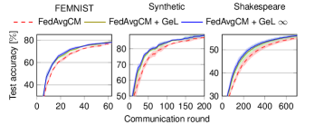
Figure 8: GeL with infinite guessed updates. Guessing too much does not hurt. Therefore, GeL does not require tuning the number of guesses.

F.2 Impact of budget range $\tau_{i}$

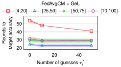
Figure 9: Impact of changing budgets on the FEMNIST dataset. $\tau^{\prime}_{i}=0$ yields the baseline FedAvgCM algorithm.

We now address the incidental question of how client budget ranges affect the performance of GeL. Intuitively, in order for guessing to be effective, GeL needs the clients to have accumulated momentum through at least some local steps. Hence, in an extreme case where clients do only one local step, GeL would be no better than the baseline. Similarly, on the other extreme where all clients manage to complete the expected amount of work, GeL would not bring significant improvements. However, in the more realistic average case, we show that GeL is effective in boosting the baseline.

We empirically confirm this by running the experiment with different ranges including [4, 20], [25, 50], [50, 75], and a wider range [10, 100] on the FEMNIST dataset. We vary the number of guesses $(\tau^{\prime}_{i})$ as [0, 10, 100] and chart the rounds to target accuracy in Figure 9. When $\tau^{\prime}_{i}=0$, we get the baseline. As we increase $\tau^{\prime}_{i}$, we control the effect of GeL. Encouragingly enough, even a large number of guesses does not lead to divergence. We observe that (i) under stringent budget conditions [4, 20], GeL speeds up convergence from 54 (baseline with 0 guesses) to 42 rounds; (ii) when the budgets increase to [25, 50], the impact of GeL reduces; (iii) when the budgets are too high [50, 75], both the baseline and GeL suffer from client drift needing more rounds than the [25, 50] case. GeL, however, does not worsen the baseline. Finally, we note that stringent resource constraints are likely to induce low-budget clients where GeL brings the most speed up.

References

- Abdelmoniem and Canini (2021) Abdelmoniem, A. M.; and Canini, M. 2021. Towards Mitigating Device Heterogeneity in Federated Learning via Adaptive Model Quantization. In 1st Workshop on Machine Learning and Systems (EuroMLSys), 96–103.
- Bergstra and Bengio (2012) Bergstra, J.; and Bengio, Y. 2012. Random Search for Hyper-Parameter Optimization. Journal of Machine Learning Research, 13(10): 281–305.
- Bonawitz et al. (2019) Bonawitz, K.; Eichner, H.; Grieskamp, W.; Huba, D.; Ingerman, A.; Ivanov, V.; Kiddon, C.; Konečný, J.; Mazzocchi, S.; McMahan, B.; Van Overveldt, T.; Petrou, D.; Ramage, D.; and Roselander, J. 2019. Towards Federated Learning at Scale: System Design. In MLSys.
- Bonawitz et al. (2016) Bonawitz, K. A.; Ivanov, V.; Kreuter, B.; Marcedone, A.; McMahan, H. B.; Patel, S.; Ramage, D.; Segal, A.; and Seth, K. 2016. Practical Secure Aggregation for Federated Learning on User-Held Data. In NIPS Workshop on Private Multi-Party Machine Learning.
- Bottou, Curtis, and Nocedal (2018) Bottou, L.; Curtis, F. E.; and Nocedal, J. 2018. Optimization methods for large-scale machine learning. Siam Review, 60(2): 223–311.
- Caldas et al. (2019) Caldas, S.; Duddu, S. M. K.; Wu, P.; Li, T.; Konečnỳ, J.; McMahan, H. B.; Smith, V.; and Talwalkar, A. 2019. Leaf: A benchmark for federated settings. In 2nd Intl. Workshop on Federated Learning for Data Privacy and Confidentiality (FL-NeurIPS).
- Charles et al. (2021) Charles, Z.; Garrett, Z.; Huo, Z.; Shmulyian, S.; and Smith, V. 2021. On large-cohort training for federated learning. Advances in neural information processing systems, 34: 20461–20475.
- Charles and Konečný (2020) Charles, Z.; and Konečný, J. 2020. On the Outsized Importance of Learning Rates in Local Update Methods. arXiv:2007.00878.
- Cutkosky and Orabona (2019) Cutkosky, A.; and Orabona, F. 2019. Momentum-Based Variance Reduction in Non-Convex SGD. In Wallach, H.; Larochelle, H.; Beygelzimer, A.; d'Alché-Buc, F.; Fox, E.; and Garnett, R., eds., Advances in Neural Information Processing Systems, volume 32. Curran Associates, Inc.
- Diao, Ding, and Tarokh (2021) Diao, E.; Ding, J.; and Tarokh, V. 2021. Hetero{FL}: Computation and Communication Efficient Federated Learning for Heterogeneous Clients. In International Conference on Learning Representations.
- Federated (2019) Federated, T. 2019. Machine Learning on Decentralized Data. TensorFlow. https://www.tensorflow.org/federated.
- Huba et al. (2022) Huba, D.; Nguyen, J.; Malik, K.; Zhu, R.; Rabbat, M.; Yousefpour, A.; Wu, C.-J.; Zhan, H.; Ustinov, P.; Srinivas, H.; Wang, K.; Shoumikhin, A.; Min, J.; and Malek, M. 2022. PAPAYA: Practical, Private, and Scalable Federated Learning. In Marculescu, D.; Chi, Y.; and Wu, C., eds., Proceedings of Machine Learning and Systems, volume 4, 814–832.
- Kairouz et al. (2020) Kairouz, P.; McMahan, H. B.; Avent, B.; Bellet, A.; Bennis, M.; Bhagoji, A. N.; Bonawitz, K.; Charles, Z.; Cormode, G.; Cummings, R.; et al. 2020. Advances and open problems in federated learning. Foundations and Trends in Machine Learning, 14(1–2).
- Karimireddy et al. (2021) Karimireddy, S. P.; Jaggi, M.; Kale, S.; Mohri, M.; Reddi, S. J.; Stich, S. U.; and Suresh, A. T. 2021. Mime: Mimicking Centralized Stochastic Algorithms in Federated Learning. arXiv:2008.03606.
- Karimireddy et al. (2020) Karimireddy, S. P.; Kale, S.; Mohri, M.; Reddi, S. J.; Stich, S. U.; and Suresh, A. T. 2020. SCAFFOLD: Stochastic Controlled Averaging for Federated Learning. In ICML.
- Keskar et al. (2017) Keskar, N. S.; Mudigere, D.; Nocedal, J.; Smelyanskiy, M.; and Tang, P. T. P. 2017. On Large-Batch Training for Deep Learning: Generalization Gap and Sharp Minima. arXiv:1609.04836.
- Khodak et al. (2021) Khodak, M.; Tu, R.; Li, T.; Li, L.; Balcan, M.-F. F.; Smith, V.; and Talwalkar, A. 2021. Federated Hyperparameter Tuning: Challenges, Baselines, and Connections to Weight-Sharing. In Ranzato, M.; Beygelzimer, A.; Dauphin, Y.; Liang, P.; and Vaughan, J. W., eds., Advances in Neural Information Processing Systems, volume 34, 19184–19197. Curran Associates, Inc.
- Kingma and Ba (2017) Kingma, D. P.; and Ba, J. 2017. Adam: A Method for Stochastic Optimization. arXiv:1412.6980.
- Lavesson and Davidsson (2006) Lavesson, N.; and Davidsson, P. 2006. Quantifying the Impact of Learning Algorithm Parameter Tuning. In Proceedings of the 21st National Conference on Artificial Intelligence - Volume 1, AAAI’06, 395–400. AAAI Press. ISBN 9781577352815.
- Li et al. (2017) Li, L.; Jamieson, K.; DeSalvo, G.; Rostamizadeh, A.; and Talwalkar, A. 2017. Hyperband: A Novel Bandit-Based Approach to Hyperparameter Optimization. J. Mach. Learn. Res., 18(1): 6765–6816.
- Li et al. (2020a) Li, T.; Sahu, A. K.; Talwalkar, A.; and Smith, V. 2020a. Federated Learning: Challenges, Methods, and Future Directions. IEEE Signal Processing Magazine, 37(3): 50–60.
- Li et al. (2020b) Li, T.; Sahu, A. K.; Zaheer, M.; Sanjabi, M.; Talwalkar, A.; and Smith, V. 2020b. Federated Optimization in Heterogeneous Networks. In MLSys.
- Li et al. (2020c) Li, Z.; Kovalev, D.; Qian, X.; and Richtárik, P. 2020c. Acceleration for Compressed Gradient Descent in Distributed and Federated Optimization. In Proceedings of the 37th International Conference on Machine Learning, ICML’20. JMLR.org.
- Mantovani et al. (2015) Mantovani, R. G.; Rossi, A. L. D.; Vanschoren, J.; Bischl, B.; and Carvalho, A. C. P. L. F. 2015. To tune or not to tune: Recommending when to adjust SVM hyper-parameters via meta-learning. In 2015 International Joint Conference on Neural Networks (IJCNN), 1–8.
- McMahan et al. (2017) McMahan, B.; Moore, E.; Ramage, D.; Hampson, S.; and y Arcas, B. A. 2017. Communication-efficient learning of deep networks from decentralized data. In AISTATS. PMLR.
- Nar and Sastry (2018) Nar, K.; and Sastry, S. S. 2018. Step Size Matters in Deep Learning. In Proceedings of the 32nd International Conference on Neural Information Processing Systems, NIPS’18, 3440–3448. Red Hook, NY, USA: Curran Associates Inc.
- Probst, Bischl, and Boulesteix (2018) Probst, P.; Bischl, B.; and Boulesteix, A.-L. 2018. Tunability: Importance of Hyperparameters of Machine Learning Algorithms. arXiv:1802.09596.
- Reddi et al. (2021) Reddi, S. J.; Charles, Z.; Zaheer, M.; Garrett, Z.; Rush, K.; Konečný, J.; Kumar, S.; and McMahan, H. B. 2021. Adaptive Federated Optimization. In International Conference on Learning Representations.
- Sattler et al. (2020) Sattler, F.; Wiedemann, S.; Müller, K.-R.; and Samek, W. 2020. Robust and Communication-Efficient Federated Learning From Non-i.i.d. Data. IEEE Transactions on Neural Networks and Learning Systems, 31(9): 3400–3413.
- So, Güler, and Avestimehr (2021) So, J.; Güler, B.; and Avestimehr, A. S. 2021. Turbo-Aggregate: Breaking the Quadratic Aggregation Barrier in Secure Federated Learning. IEEE Journal on Selected Areas in Information Theory, 2(1): 479–489.
- Sutskever et al. (2013) Sutskever, I.; Martens, J.; Dahl, G.; and Hinton, G. 2013. On the importance of initialization and momentum in deep learning. In Dasgupta, S.; and McAllester, D., eds., Proceedings of the 30th International Conference on Machine Learning, Proceedings of Machine Learning Research, 1139–1147. Atlanta, Georgia, USA: PMLR.
- Wang et al. (2018) Wang, H.; Sievert, S.; Liu, S.; Charles, Z.; Papailiopoulos, D.; and Wright, S. 2018. ATOMO: Communication-efficient Learning via Atomic Sparsification. In Bengio, S.; Wallach, H.; Larochelle, H.; Grauman, K.; Cesa-Bianchi, N.; and Garnett, R., eds., Advances in Neural Information Processing Systems, volume 31. Curran Associates, Inc.
- Wang et al. (2021) Wang, J.; Charles, Z.; Xu, Z.; Joshi, G.; McMahan, H. B.; y Arcas, B. A.; Al-Shedivat, M.; Andrew, G.; Avestimehr, S.; Daly, K.; Data, D.; Diggavi, S.; Eichner, H.; Gadhikar, A.; Garrett, Z.; Girgis, A. M.; Hanzely, F.; Hard, A.; He, C.; Horvath, S.; Huo, Z.; Ingerman, A.; Jaggi, M.; Javidi, T.; Kairouz, P.; Kale, S.; Karimireddy, S. P.; Konecny, J.; Koyejo, S.; Li, T.; Liu, L.; Mohri, M.; Qi, H.; Reddi, S. J.; Richtarik, P.; Singhal, K.; Smith, V.; Soltanolkotabi, M.; Song, W.; Suresh, A. T.; Stich, S. U.; Talwalkar, A.; Wang, H.; Woodworth, B.; Wu, S.; Yu, F. X.; Yuan, H.; Zaheer, M.; Zhang, M.; Zhang, T.; Zheng, C.; Zhu, C.; and Zhu, W. 2021. A Field Guide to Federated Optimization. arXiv:2107.06917.
- Wang et al. (2020) Wang, J.; Liu, Q.; Liang, H.; Joshi, G.; and Poor, H. V. 2020. Tackling the Objective Inconsistency Problem in Heterogeneous Federated Optimization. In NeurIPS.
- Weerts, Mueller, and Vanschoren (2020) Weerts, H. J. P.; Mueller, A. C.; and Vanschoren, J. 2020. Importance of Tuning Hyperparameters of Machine Learning Algorithms. arXiv:2007.07588.
- Wei et al. (2020) Wei, K.; Li, J.; Ding, M.; Ma, C.; Yang, H. H.; Farokhi, F.; Jin, S.; Quek, T. Q. S.; and Poor, H. V. 2020. Federated Learning With Differential Privacy: Algorithms and Performance Analysis. IEEE Transactions on Information Forensics and Security, 15: 3454–3469.
- Wu, Ma, and E (2018) Wu, L.; Ma, C.; and E, W. 2018. How SGD Selects the Global Minima in Over-parameterized Learning: A Dynamical Stability Perspective. In Bengio, S.; Wallach, H.; Larochelle, H.; Grauman, K.; Cesa-Bianchi, N.; and Garnett, R., eds., Advances in Neural Information Processing Systems, volume 31. Curran Associates, Inc.
- Yang et al. (2021) Yang, C.; Wang, Q.; Xu, M.; Chen, Z.; Bian, K.; Liu, Y.; and Liu, X. 2021. Characterizing Impacts of Heterogeneity in Federated Learning upon Large-Scale Smartphone Data. In Proceedings of the Web Conference 2021, 935–946.
- Yang et al. (2018) Yang, T.; Andrew, G.; Eichner, H.; Sun, H.; Li, W.; Kong, N.; Ramage, D.; and Beaufays, F. 2018. Applied Federated Learning: Improving Google Keyboard Query Suggestions. arXiv:1812.02903.
- Zaheer et al. (2018) Zaheer, M.; Reddi, S.; Sachan, D.; Kale, S.; and Kumar, S. 2018. Adaptive Methods for Nonconvex Optimization. In Bengio, S.; Wallach, H.; Larochelle, H.; Grauman, K.; Cesa-Bianchi, N.; and Garnett, R., eds., Advances in Neural Information Processing Systems, volume 31. Curran Associates, Inc.
- Zhou et al. (2021) Zhou, G.; Xu, K.; Li, Q.; Liu, Y.; and Zhao, Y. 2021. AdaptCL: Efficient Collaborative Learning with Dynamic and Adaptive Pruning. arXiv:2106.14126.
- Zhou et al. (2023) Zhou, Y.; Ram, P.; Salonidis, T.; Baracaldo, N.; Samulowitz, H.; and Ludwig, H. 2023. Single-shot General Hyper-parameter Optimization for Federated Learning. In The Eleventh International Conference on Learning Representations.