Valley and spin accumulation in ballistic and hydrodynamic channels

Abstract

A theory of the valley and spin Hall effects and resulting accumulation of the valley and spin polarization is developed for ultraclean channels made of two-dimensional semiconductors where the electron mean free path due to the residual disorder or phonons exceeds the channel width. Both ballistic and hydrodynamic regimes of the electron transport are studied. The polarization accumulation is determined by interplay of the anomalous velocity, side-jump and skew scattering effects. In the hydrodynamic regime, where the electron-electron scattering is dominant, the valley and spin current generation and dissipation by the electron-electron collisions are taken into account. The accumulated polarization magnitude and its spatial distribution depend strongly on the transport regime. The polarization is much larger in the hydrodynamic regime as compared to the ballistic one. Significant valley and spin polarization arises in the immediate vicinity of the channel edges due to the side-jump and skew scattering mechanisms.

I Introduction

Transport of spin and valley degrees of freedom is of particular interest owing to fascinating fundamental physics Dyakonov (2017); Dyakonov and Perel’ (1971a, b); Hirsch (1999); Murakami et al. (2003); Sinova et al. (2004); Wunderlich et al. (2005); Kavokin et al. (2005); Leyder et al. (2007); Mak et al. (2014); Ubrig et al. (2017); Lundt et al. (2019). Spin-orbit interaction drives anomalous transport where the electric current transversal to the external electric field is generated in spin-polarized media Hall (1881); Nagaosa et al. (2010) and related phenomena, particularly, the spin Hall effect (SHE) and valley Hall effect (VHE). Because of the VHE, the particles in different valleys of the Brillouin zone propagate in opposite directions and accumulate at the opposite edges of the sample. The VHE can be used for non-magnetic valley manipulation.

The rise of a novel material system, transition metal dichalcogenide monolayers Mak et al. (2010); Splendiani et al. (2010); Kormanyos et al. (2015); Kolobov and Tominaga (2016); Wang et al. (2018) with multivalley band structure, spin-valley locking and chiral selection rules for optical transitions Xiao et al. (2012); Mak et al. (2012); Xu et al. (2014) boosted experimental and theoretical studies of the VHE Xiao et al. (2012); Mak et al. (2014); Konabe and Yamamoto (2014); Jin et al. (2018); Onga et al. (2017); Unuchek et al. (2019); Lundt et al. (2019); Kulig et al. (2018); Kalameitsev et al. (2019); Ubrig et al. (2017); Glazov and Golub (2020a, b). The microscopic mechanisms of the effect have been debated in the literature until recently. However, in Refs. Glazov and Golub (2020a, b) we have shown that regardless the origin of the drag force – caused by the real or synthetic electric field, phonon or photon drag, or the Seebeck effect – which results in the direct flow of the particles, the VHE is related solely to the scattering. Namely, the asymmetric or skew scattering by impurities and phonons and the side-jumps in the course of the scattering result in the valley current transversal to the direct current and eventually lead to the valley accumulation at the sample edges. The anomalous velocity arising in the presence of the external potential field Xiao et al. (2010); Kuga et al. (2008); Yao and Niu (2008); Xiao et al. (2012); Li et al. (2015); Onga et al. (2017); Kalameitsev et al. (2019); Kovalev and Savenko (2019); Gianfrate et al. (2020), e.g., where the current is induced by the electric field, is compensated by the part of the side-jump contribution, that is by the anomalous velocity resulting from defect or phonon-induced force field. Similar compensation takes place for the spin Hall effect in semiconductors as well Dyakonov (2017); Sinitsyn et al. (2007); Sinitsyn (2007); Ado et al. (2015).

Recent progress in nanotechnology has made it possible to create two-dimensional electron systems with ultrahigh mobility where the electron mean free path $l$ exceeds by far the width of the channel $w$ de Jong and Molenkamp (1995); Titov et al. (2013); Bandurin et al. (2016); Moll et al. (2016); Gusev et al. (2018); Krishna Kumar et al. (2017); Ku et al. (2020); Sulpizio et al. (2019); Berdyugin et al. (2019); Gusev et al. (2020). In this case, the electron momentum dissipation takes place mainly at the channel edges. Moreover, the electron-electron interaction can give rise to a novel – hydrodynamic – regime of the electron transport where electrons behave collectively as a viscous fluid Gurzhi (1963, 1968); Müller et al. (2009); Andreev et al. (2011); Torre et al. (2015); Pellegrino et al. (2017); Narozhny et al. (2015); Alekseev (2016); Levitov and Falkovich (2016); Kashuba et al. (2018); Lucas (2017), see Refs. Narozhny et al. (2017); Lucas and Fong (2018) for review and Refs. Alekseev et al. (2018); Alekseev and Semina (2018, 2019) for discussion of other non-diffusive regimes of the electron transport in ultraclean channels. Description of anomalous transport in such ultrahigh mobility systems is a pressing problem. In recent works Apostolov et al. (2019); Hasdeo et al. (2021); Funaki et al. (2021); tatara1 some aspects of the electron anomalous transport have been addressed, however, the consistent theory of the VHE and SHE in the ballistic and hydrodynamic regimes is absent to the best of our knowledge. Our paper aims to fill this gap.

Here we present the theory of the valley and spin Hall effects and accumulation of polarization in electron channels with long mean free path, $l\gg w$, addressing both ballistic (where electron-electron collisions are unimportant) and hydrodynamic (where the electron-electron scattering length $l_{ee}\ll w$) transport regimes. We calculate all contributions to the VHE and SHE: skew-scattering, side-jump, and anomalous velocity, and discuss their interplay. We uncover the role of the scattering by the sample edges and introduce the impurity stripe model to address the edge scattering microscopically. We study a role of electron-electron collisions in the valley current generation and dissipation. We demonstrate that different mechanisms of the VHE and SHE can manifest themselves in the different parts of the channel.

The paper is organized as follows. After brief introduction in Sec. I, we present in Sec. II the basic description of the normal electron transport in ultraclean channels outlining the ballistic and hydrodynamic regimes. We also present a model of the impurity stripes (Sec. II.2) enabling simple microscopic approach to the edge scattering. Section III contains the theory of the VHE and SHE and polarization accumulation inside the channel. Both ballistic (Sec. III.2) and hydrodynamic (Sec. III.4) regimes are addressed. The electron-electron scattering effects on the spin and valley current relaxation and generation are addressed in Sec. III.3. In Sec. IV the spin and valley accumulation in the impurity stripes is studied. The obtained results are summarized in Sec. V and the paper is concluded with Sec. VI.

II Electron transport in ultraclean channels

This section contains preliminaries about the normal electron transport in narrow channels. In particular, we present the model of the diffusive scattering at the channel edges and calculate the electron distribution function in the presence of the longitudinal electric field and the longitudinal conductivity both in the ballistic and in hydrodynamic regimes.

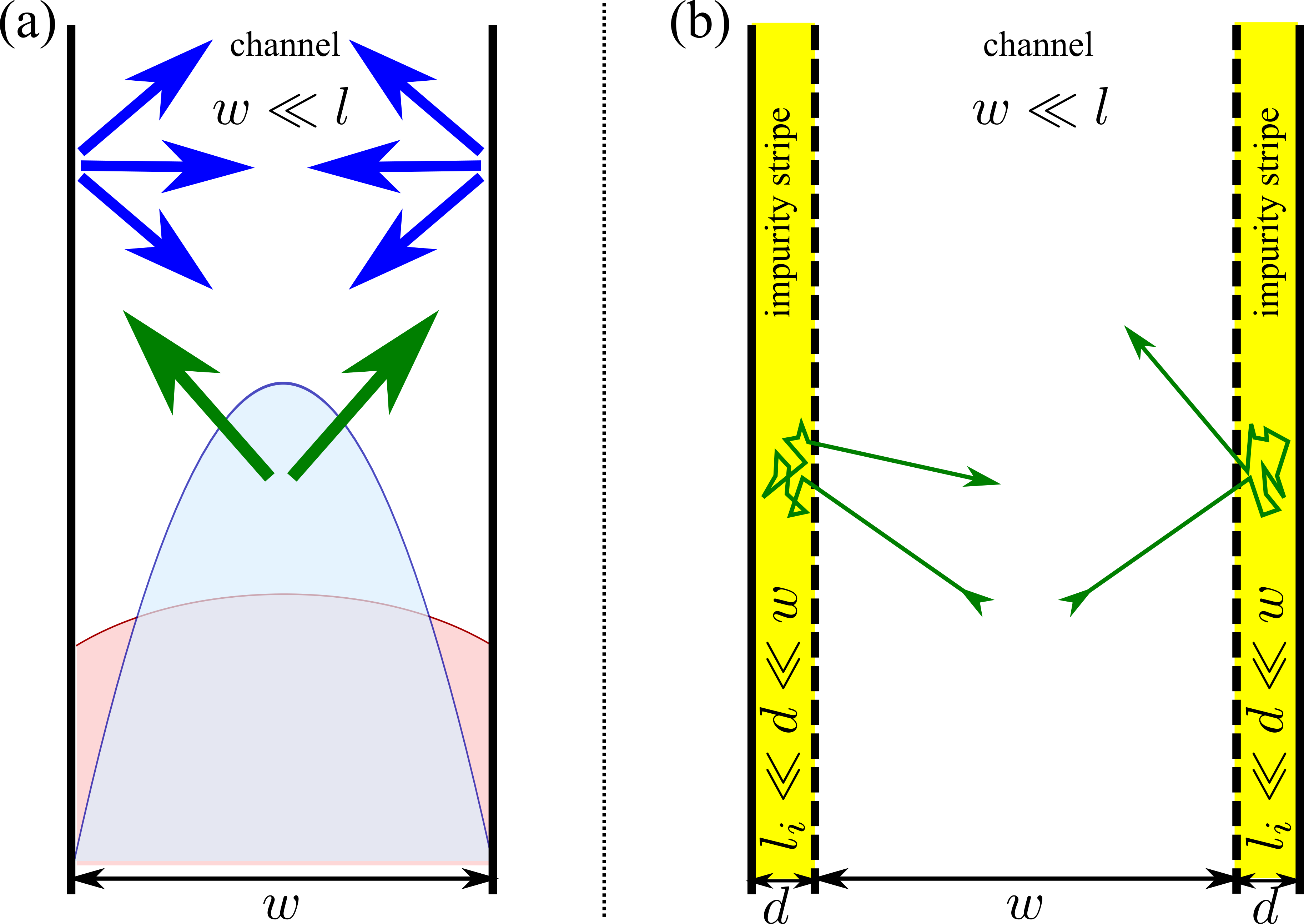
Figure 1: (a) Schematic illustration of the narrow channel and diffusive scattering at the edges. Green arrows show the directions of incident electron velocities and blue arrows show the directions of the scattered electrons velocities. Light red and blue profiles show the steady-state distribution of the electron velocity in the ballistic and hydrodynamic regimes, respectively. (b) Model of the impurity stripes shown by yellow areas at the channel edges. Green lines show typical electron trajectories: ballistic inside the channel and diffusive in the impurity stripes.

II.1 Diffusive scattering

We consider a channel with the two-dimensional electron gas, Fig. 1(a). The motion of electrons is bounded along the $x$-axis and the motion along the $y$-axis is free. We assume that the channel width $w$ is by far smaller than the electron mean free path $l$ caused by the scattering by a static short-range disorder. In this regime, the main source of the electron momentum relaxation is the scattering by the edges of the channel. Usually, a phenomenological description of diffusive edge scattering is employed where the following boundary condition for the electron distribution function $f_{\bm{p}}(x)$ is used Fuchs (1938); Reuter and Sondheimer (1948); Fal’kovskii (1970):

$$f_{\bm{p}}(\pm w/2)=\begin{cases}\mathrm{const},\leavevmode\nobreak\ \leavevmode\nobreak\ p_{x}>0,\leavevmode\nobreak\ \leavevmode\nobreak\ x=-w/2,\\ \mathrm{const},\leavevmode\nobreak\ \leavevmode\nobreak\ p_{x}<0,\leavevmode\nobreak\ \leavevmode\nobreak\ x=w/2.\end{cases}$$ (1)

Here $\bm{p}$ is the electron wavevector. This condition means that the electrons travelling from the edge, i.e., scattered by the edge, have random directions of their momentum as shown in Fig. 1(a).

In the presence of the static electric field $\bm{E}\parallel y$ the electron distribution function acquires a linear-in-$\bm{E}$ correction which can be found from the kinetic equation ll10_eng ; Fal’kovskii (1970)

$$v_{x}\frac{\partial\delta f_{\bm{p}}(x)}{\partial x}+\frac{\delta f_{\bm{p}}(x)}{\tau}-eE_{y}v_{y}f_{0}^{\prime}=Q_{ee}\{\delta f_{\bm{p}}\},$$ (2)

where $\bm{v}=(v_{x},v_{y})=\hbar\bm{p}/m$ is the electron velocity, $m$ is its effective mass, $\tau$ is the momentum relaxation time (related to the residual impurities or phonons), $f_{0}$ is the equilibrium Fermi-Dirac distribution function, and prime denotes the derivative over the energy. The quantity $Q_{ee}\{\delta f_{\bm{p}}\}$ in the right-hand side is the electron-electron collision integral.

We start from the ballistic regime where the electron-electron scattering can be neglected, $Q_{ee}\{\delta f_{\bm{p}}\}=0$. The solution of Eq. (2) with the boundary condition (1) readily yields

$$\delta f_{\bm{p}}(x)=eE_{y}l(-f_{0}^{\prime})\sin{\varphi_{\bm{p}}}\\ \times\quantity{1-\exp[-{{x+\text{sgn}(\cos{\varphi_{\bm{p}}})w/2}\over l\cos{\varphi_{\bm{p}}}}]}.$$ (3)

Here $\varphi_{\bm{p}}$ is the angle between the momentum and $x$-axis, $l=v\tau$ is the mean free path in respect to the scattering in the “bulk” of the sample.

In the narrow ultraclean channels with $w\ll l$, we have from Eq. (3) up to the first order in $w/l$:

$$\delta f_{\bm{p}}(x)\approx eE_{y}(-f_{0}^{\prime})\sin{\varphi_{\bm{p}}}{{x+\text{sgn}(\cos{\varphi_{\bm{p}}})w/2}\over\cos{\varphi_{\bm{p}}}}.$$ (4)

In this regime the channel conductivity relating the two-dimensional current density ($\mathcal{L}$ is the normalization length along the $y$-axis)

$$j_{y}=\frac{1}{w\mathcal{L}}\int_{-w/2}^{w/2}\sum_{\bm{p}}v_{y}\delta f_{\bm{p}}(x)dx,$$ (5)

with the electric field component $E_{y}$ as

$$j_{y}=\sigma_{yy}E_{y}$$ (6)

takes the following form:

$$\sigma_{yy}^{b}=\frac{2}{\pi}\sigma_{0}\frac{w}{l}\ln{\left(\frac{l}{w}\right)},\quad\sigma_{0}=\frac{e^{2}N\tau}{m},$$ (7)

Here and in what follows we omit the factor describing the spin and valley degeneracy of the electron states, $N$ is the total two-dimensional electron density.

Equation (7) shows that the channel width $w$ plays a role of the effective mean free path $l_{\rm eff}$. Strictly speaking, $l_{\rm eff}\sim w\ln{(l/w)}$. The logarithmic factor $\ln{(l/w)}$ accounts for the contribution of the electrons at the grazing incidence at the edges: These electrons travel large distance $\sim w/\cos{\varphi_{\bm{p}}}$ between the consecutive collisions between the edges.

The analysis above is valid for a ballistic channel. Let us now turn to the opposite limit of very strong electron-electron scattering where the hydrodynamic regime is realized. Here we assume that (i) the relaxation of the second angular harmonic of the distribution function is controlled by frequent electron-electron collisions and (ii) the corresponding relaxation length $l_{2}\equiv l_{ee}={v\tau_{ee}}$, where $\tau_{ee}$ is the electron-electron scattering time, is the smallest parameter of the problem: $l_{2}\ll w\ll l$. In this situation we can keep only first and second angular harmonics in the electron distribution function $\delta f_{\bm{p}}(x)$ Gurzhi (1968):

$$\delta f_{\bm{p}}(x)=\sin{\varphi_{\bm{p}}}\,F_{1}^{s}(x)+\sin{2\varphi_{\bm{p}}}\,F_{2}^{s}(x),$$ (8)

where $F_{n}^{s}(x)$ are the coordinate-dependent harmonics of the distribution function whose dependence on the electron energy is omitted for brevity. In the presence of electric field $\bm{E}\parallel y$ we have the following set of coupled equations

$$\frac{l}{2}\frac{\partial F_{2}^{s}}{\partial x}+F_{1}^{s}=-eE_{y}lf_{0}^{\prime},\quad\frac{l_{2}}{2}\frac{\partial F_{1}^{s}}{\partial x}+F_{2}^{s}=0.$$ (9)

We stress that $l$ here is due to the residual disorder and $l_{2}$ is due to the electron-electron scattering. Equations (9) can be conveniently combined into one equation for $F_{1}^{s}(x)$:

$$-\eta\frac{\partial^{2}F_{1}^{s}}{\partial x^{2}}+\frac{F_{1}^{s}}{\tau}=-evE_{y}f_{0}^{\prime},$$ (10)

where the viscosity

$$\eta=\frac{vl_{2}}{4}.$$ (11)

In what follows we completely neglect the disorder in the channel setting $\tau\to\infty$. Hence, following Refs. Gurzhi (1968); Alekseev (2016) we obtain

$$\delta f_{\bm{p}}(x)=-\frac{eE_{y}v_{y}f_{0}^{\prime}}{2\eta}\left\{\left[\left(\frac{w}{2}\right)^{2}-x^{2}\right]+\frac{2l_{2}v_{x}}{v}x\right\}.$$ (12)

Naturally, Eq. (12) contains the first and second angular harmonics of the distribution function; as expected, the second harmonic is much smaller than the first one. The electron velocity distribution corresponds in this case to the Poiseuille flow. Accordingly, the longitudinal conductivity can be written as Alekseev (2016)

$$\sigma_{yy}^{h}=\sigma_{0}\frac{w^{2}}{12\eta\tau}.$$ (13)

Here the role of grazing electrons is drastically reduced because of the electron-electron collisions: Although conserving the total momentum of the colliding pair, they efficiently change the incidence angle of the electron at the edge. In the hydrodynamic regime the role of the effective mean free path is played by $l_{\rm eff}\sim w^{2}/l_{2}\gg w$ yielding $\sigma^{h}_{yy}\gg\sigma^{b}_{yy}$. This relation is natural, because due to the efficient electron-electron collisions for the most of electrons the momentum dissipation is indirect and, hence, inefficient: Via multiple collisions, the momentum is transferred from electrons in the bulk of the channel to those near the edges where the dissipation occurs. The smaller $l_{2}$ is, the more efficient is the suppression of the edge scattering resulting in larger conductivity $\sigma^{h}_{yy}$.

II.2 Impurity stripe model

Microscopic derivation of the diffusive boundary condition (1) is quite involved Greene (1966); Fal’kovskii (1970); Andreev (1972); Pellegrino et al. (2017); Kiselev and Schmalian (2019). On the other hand, as we demonstrate below, the edge scattering is crucial for the anomalous transport and VHE. Thus, it is instructive to introduce a simple model of the edge which allows us to derive the results above without explicit use of Eq. (1). To that end we introduce the impurity stripe model of the edge: We assume that there are narrow stripes of the width $d\ll w$ in the vicinity of each edge with high concentration of the scattering centers, i.e., impurities, so that the mean free path in these impurity stripes $l_{i}=v\tau_{i}\ll d$ ($\tau_{i}$ is the electron scattering time in the impurity stripe), Fig. 1(b). We also assume that the electron-electron scattering is irrelevant in the impurity stripe, $\tau_{i}\ll\tau_{ee}$. Thus, the electron motion in the impurity stripe is diffusive rather than ballistic. At the same time, the boundary conditions at the outer edges of the impurity stripes are unimportant and, for simplicity, we can assume specular reflection from these edges. Corresponding distribution functions can be found solving the kinetic equation (2) in different regions of the channel and joining the solutions at $x=\pm w/2$.

In the limit $l_{i}\to 0$ the solution for the $\delta f_{\bm{p}}$ within the channel, Eq. (3) (in the ballistic regime) or Eq. (12) (in the hydrodynamic regime), is not affected by the presence of the impurity stripes. By contrast, within the impurity stripes we obtain

$$\delta f_{\bm{p}}(x)=-eE_{y}l_{i}f_{0}^{\prime}\sin{\varphi_{\bm{p}}}\\ +\begin{cases}{\delta}f_{\bm{p}}^{<}(x),\quad-d-\frac{w}{2}\leqslant x\leqslant-\frac{w}{2},\\ {\delta}f_{\bm{p}}^{>}(x),\quad\frac{w}{2}\leqslant x\leqslant\frac{w}{2}+d,\end{cases}$$ (14)

where for the ballistic channel ($w\ll l$)

$${\delta}f_{\bm{p}}^{<,b}(x)=eE_{y}l_{i}f_{0}^{\prime}\frac{\sin{\varphi_{\bm{p}}}}{\cos{\varphi_{\bm{p}}}}\\ \times\begin{cases}0,\quad v_{x}>0,\\ \frac{w}{l_{i}}\exp[\left(-\frac{x+w/2}{l_{i}\cos{\varphi_{\bm{p}}}}\right)],\quad v_{x}<0,\end{cases}$$ (15a)

while for the hydrodynamic channel

$${\delta}f_{\bm{p}}^{<,h}(x)=eE_{y}l_{i}f_{0}^{\prime}\sin{\varphi_{\bm{p}}}\cos{\varphi_{\bm{p}}}\\ \times\begin{cases}0,\quad v_{x}>0,\\ \frac{4w}{l_{i}}\exp[\left(-\frac{x+w/2}{l_{i}\cos{\varphi_{\bm{p}}}}\right)],\quad v_{x}<0,\end{cases}$$ (15b)

Within the stripe at the right edge of the channel the solution $\delta f^{>}_{\bm{p}}(x)$ can be obtained from Eq. (15) by natural replacements $w/2\to-w/2$, $v_{x}\to-v_{x}$:

$${\delta}f_{\bm{p}}^{>,b}(x)=-eE_{y}l_{i}f_{0}^{\prime}\frac{\sin{\varphi_{\bm{p}}}}{\cos{\varphi_{\bm{p}}}}\\ \times\begin{cases}0,\quad v_{x}<0,\\ \frac{w}{l_{i}}\exp\left(-\frac{x-w/2}{l_{i}\cos{\varphi_{\bm{p}}}}\right),\quad v_{x}>0,\end{cases}$$ (16a)

and

$${\delta}f_{\bm{p}}^{>,h}(x)=-eE_{y}l_{i}f_{0}^{\prime}\sin{\varphi_{\bm{p}}}\cos{\varphi_{\bm{p}}}\\ \times\begin{cases}0,\quad v_{x}<0,\\ \frac{4w}{l_{i}}\exp\left(-\frac{x-w/2}{l_{i}\cos{\varphi_{\bm{p}}}}\right),\quad v_{x}>0,\end{cases}$$ (16b)

Up to $l_{i}/l\ll 1$ corrections, the distribution function is continuous at $x=\pm w/2$. One can check that the contributions of the impurity stripes to the channels conductivity are negligible at $d\ll w$. Note that in the case of ballistic channel corresponding expressions (15a) and (16a) are inapplicable for grazing angles where $|\cos{\varphi_{\bm{p}}}|\lesssim w/l$. In such situation the ratio $\sin{\varphi_{\bm{p}}}/\cos{\varphi_{\bm{p}}}$ should be replaced by the full expression [cf. Eq. (3)]

$$\frac{\sin{\varphi_{\bm{p}}}}{|\cos{\varphi_{\bm{p}}}|}\to\sin{\varphi_{\bm{p}}}\left[1-\exp(-{w\over l|\cos{\varphi_{\bm{p}}}|})\right].$$ (17)

The first term in Eq. (14) is responsible for the field-induced electric current in the stripe. The second contribution, ${\delta}f_{\bm{p}}^{<}(x)$, is related to the electrons entering the impurity stripe from the channel. One can check that this contribution is responsible for the momentum dissipation in the channel. Indeed, the momentum loss per unit length in both impurity stripes takes the form

$$\dot{P}_{y}=\frac{2}{\mathcal{L}}\int_{-w/2-d}^{-w/2}\sum_{\bm{p}\bm{p}^{\prime}}{\delta}f_{\bm{p}}^{<}(x)(p^{\prime}_{y}-p_{y})W^{(i)}_{\bm{p}^{\prime},\bm{p}}dx,$$ (18)

where the factor $2$ accounts for both left and right stripes, Fig. 1(b), and $W^{(i)}_{\bm{p}^{\prime},\bm{p}}$ is the rate of the transitions from the state $\bm{p}\to\bm{p}^{\prime}$ in the impurity stripe due to the scattering. Evaluating the integral and sum in Eq. (18) we obtain

$$\dot{P_{y}}=-eE_{y}Nw,$$ (19)

which equals to the electric force (per unit length) applied to the electrons in the channel taken with the opposite sign.

III Valley Hall effect in the channel

III.1 Mechanisms of the VHE and SHE

We now turn to the anomalous transport of electrons and study the valley and spin Hall effects. We employ the model discussed in Ref. Glazov and Golub (2020a) and consider the transition metal dichalcogenide monolayer with two valleys $\bm{K}_{\pm}$ in the Brillouin zone. In the case of the spin Hall effect, the spin-up, $\uparrow$, and spin-down, $\downarrow$, states can be mapped onto the valleys $\bm{K}_{+}$ and $\bm{K}_{-}$ because of the same properties of the corresponding Bloch functions under time-reversal. For specificity, in what follows, we use the term valley and discuss valley currents and valley polarization accumulation bearing in mind that the same results hold for the spin currents and spin polarization accumulation. The effective Hamiltonian in the corresponding valley in the simplest two-band approximation (two-dimensional Dirac model) takes the form Xiao et al. (2012); Kormanyos et al. (2015)

$$\mathcal{H}_{\pm}=\begin{bmatrix}0&\pm\gamma k_{\mp}\\ \pm\gamma k_{\pm}&-E_{g}\end{bmatrix},\quad\gamma=\frac{\hbar p_{cv}}{m_{0}}{\in\mathbb{R}.}$$ (20)

Here $E_{g}$ is the bandgap, $p_{cv}$ is the interband momentum matrix element, $k_{\pm}=k_{x}\pm\mathrm{i}k_{y}$, $x$ and $y$ are the axes in the 2D plane. The same model can be used for the SHE since the Hamiltonians $\mathcal{H}_{\pm}$ in Eq. (20) describes two spin branches in a quantum well. Importantly, the band mixing is chiral and depends on the valley or spin branch: For the one state ($\bm{K}_{+}$ or spin-$\uparrow$) the coupling is $\propto k_{x}-\mathrm{i}k_{y}$, and for the other state ($\bm{K}_{-}$ or spin-$\downarrow$) it is $\propto k_{x}+\mathrm{i}k_{y}$. In quantum wells such form of the two-band Hamiltonian is a direct consequence of the spin-orbit coupling in the valence band, heavy-light hole splitting, and the $\bm{k}\cdot\bm{p}$-mixing of the bands ivchenko05a . In the case of transition-metal dichalcogenides it results from the specific form of the Bloch functions at the $\bm{K}_{\pm}$ points stemming from the broken sublattice symmetry and can be considered as an effective valley-orbit coupling. The generalization of the model to account for both spin and valley degrees of freedom is straightforward. In what follows we consider degenerate electrons with the Fermi energy $\varepsilon_{F}$ reckoned from the conduction band mininum being small as compared to $E_{g}$ and spin-orbit splitting of the bands. Hence, we include the interband mixing in the lowest non-vanishing order in $\gamma k/E_{g}$. We also assume that the electrons scatter by a residual static short-range disorder with the potential in the conduction band, $V_{c}(\bm{r})$, and in the valence band, $V_{v}(\bm{r})$, given by

$$V_{c,v}(\bm{r})=\sum_{i}U_{c,v}\delta(\bm{r}-\bm{R}_{i}),$$ (21)

where $\bm{R}_{i}$ are the random positions of the defects, and $U_{c,v}$ are the parameters describing the scattering potential in the conduction $U_{c}$ and valence $U_{v}$ bands, respectively. For the screened Coulomb impurities $U_{c}=U_{v}$. The disorder-induced momentum relaxation rate can be calculated using the Fermi’s golden rule ll3_eng $\tau^{-1}=(2\pi/\hbar)N_{imp}\sum_{\bm{k}^{\prime}}|U_{c}|^{2}\delta(\varepsilon_{k}-\varepsilon_{k}^{\prime})$ with $\varepsilon_{k}={\hbar^{2}k^{2}}/{2m}$ being the electron kinetic energy, $m$ its effective mass, and reads daviesBOOK

$$\frac{1}{\tau}=\frac{2\pi}{\hbar}g|U_{c}|^{2}N_{imp},$$ (22)

where $g=m/(2\pi\hbar^{2})$ is the density of states (per valley) and $N_{imp}$ is the density of the residual impurities.

The analysis shows that there are the following contributions to the VHE and SHE Sinitsyn et al. (2007); Sinitsyn (2007); Ado et al. (2015); Glazov and Golub (2020a) (we present the expressions for the $\bm{K}_{+}$ valley or spin-$\uparrow$, the expressions for the $\bm{K}_{-}$ valley or spin-$\downarrow$ differ by the sign):

1. Anomalous velocity contribution

   $$\bm{v}_{a}=-{2\xi e\over\hbar}\hat{\bm{z}}\times\bm{E},\quad\xi=\frac{\gamma^{2}}{E_{g}^{{2}}},$$ (23)

   arising in the external electric field.

2. Side-jump accumulation contribution related to the electron wavepacket shift at the scattering  Karplus and Luttinger (1954); Belinicher et al. (1982); Sturman (2019); Glazov and Golub (2020a).

   $$\bm{R}_{\bm{k}^{\prime}\bm{k}}\equiv(X_{\bm{k}^{\prime}\bm{k}},Y_{\bm{k}^{\prime}\bm{k}})\\ =\xi\frac{U_{v}}{U_{c}}[(\bm{k}^{\prime}-\bm{k})\times\hat{\bm{z}}]+\xi[(\bm{k}^{\prime}-\bm{k})\times\hat{\bm{z}}],$$ (24)

   resulting in the anomalous side-jump current $\propto\sum_{\bm{k}\bm{k}^{\prime}}W_{\bm{k}\bm{k}^{\prime}}\bm{R}_{\bm{k}^{\prime}\bm{k}}$ with $W_{\bm{k}\bm{k}^{\prime}}$ being the electron scattering rate. The first term in Eq. (24) is associated with the wavevector dependence of the matrix element phase and the second term in responsible for the Bloch electron coordinate.

3. Side-jump contribution related the anomalous distribution formed as a result of the work of the electric field $e\bm{E}\bm{R}_{\bm{k}^{\prime}\bm{k}}$ in the course of scattering which results in the scattering asymmetry.

4. The skew (asymmetric) scattering by single impurities or impurity pairs (coherent scattering) characterized by the asymmetric scattering probability

   $$W_{\bm{k}^{\prime}\bm{k}}^{as}=\xi S_{imp}[\bm{k}\times\bm{k}^{\prime}]_{z}\delta(\varepsilon_{k}-\varepsilon_{k^{\prime}}),$$ (25)

   with

   $$S_{imp}={{2\pi}U_{v}\over\tau}-\frac{U_{v}}{U_{c}}\frac{\hbar}{g\varepsilon_{k}\tau^{2}}.$$ (26)

   Here the first term is responsible for the skew-scattering by single impurity, while the second term describes the two-impurity coherent scattering Glazov and Golub (2020a); Ado et al. (2015).

Importantly, the parameter $\xi$ introduced in Eq. (23) controls the strength of the effective valley- or spin-orbit coupling; accordingly the spin and valley Hall effects are proportional to $\xi$. Hereafter we consider only $\xi$-linear regime.

While in diffusive systems the anomalous velocity contribution 1 is compensated by a part of the side-jump contributions 2, 3 Dyakonov (2017); Sinitsyn et al. (2007); Glazov and Golub (2020a, b), for narrow channels, as we show below, such compensation generally is absent and all effects should be taken into account.

We stress that the mechanisms 1–4 result in the valley or spin current flowing in the bulk of the sample (along the $x$-axis in the geometry of Fig. 1). However, the current cannot flow through the sample edges, and it should be compensated by the “diffusive” current which arises due to the accumulated valley polarization. The theory for the “bulk” spin or valley Hall conductivity developed in Ref. Glazov and Golub (2020a) and standard model of the polarization accumulation at the sample edges Dyakonov and Perel’ (1971b, a); Dyakonov (2017) cannot be directly applied to our situation because the motion of the electrons is ballistic rather than diffusive. Hence, our goal is to find the steady-state distribution of the electron valley polarization across the narrow channel accounting for all the contributions to the valley Hall effect introduced above.

To find the valley (spin) polarization we apply the generalized kinetic equation for the distribution function which accounts for also the anomalous contributions to the electron velocity. Namely, we introduce $\Delta f_{\bm{p}}^{\pm}(x)$, the non-equilibrium part of the distribution function related to the valley Hall effect in the $\bm{K}_{\pm}$ valley. In the case of SHE signs $\pm$ denote the spin branches. Note that this part of the distribution function is even at $k_{y}\to-k_{y}$ in our geometry, in contrast to the part $\delta f_{\bm{p}}$ introduced in Sec. II and arising as a linear (normal) response to the electric field $\bm{E}\parallel y$, see Fig. 1. Naturally, $\Delta f_{\bm{p}}^{+}(x)=-\Delta f_{\bm{p}}^{-}(x)$. Since we are interested in the effects at sufficiently low temperatures where the electron gas is degenerate, the energy dependence of $\Delta f_{\bm{p}}^{\pm}(x)$ is unimportant. Thus, it is convenient to introduce the energy-integrated distribution function which depends on the direction of the momentum $\varphi$ and coordinate $x$ only:

$$\Delta F_{\varphi}^{\pm}(x)=g\int_{0}^{\infty}\Delta f_{\bm{p}}^{\pm}(x)d\varepsilon_{p}.$$ (27)

Accordingly, the kinetic equation takes the form [cf. Refs. Sundaram and Niu (1999); Sekine and Nagaosa (2020); König and Levchenko (2021)]

$$\frac{\partial}{\partial x}\left[v_{x}\Delta F_{\varphi}^{\pm}(x)+\left(v_{a}^{\pm}+v_{sj}^{\pm}\right)N_{1}\right]+\frac{\Delta F_{\varphi}^{\pm}-\overline{\Delta F_{\varphi}^{\pm}}}{\tau}\\ =Q_{ee}\{\Delta F^{\pm}_{\varphi}\}+G^{\pm}(\varphi,x).$$ (28)

Here $v_{x}=v\cos{\varphi}$ where $v$ is the Fermi velocity, $N_{1}$ is the electron density per valley, $v_{sj}^{\pm}{\equiv v_{sj}^{\pm}(x)}$ is the contribution to the anomalous velocity caused by the side-jump, overline denotes the averaging over angle $\varphi$ of the electron momentum, and

$${G^{\pm}(\varphi,x)=G_{sk}^{\pm}(\varphi,x)+G_{adist}^{\pm}(\varphi,x),}$$ (29)

is the generation rate due to (i) the skew scattering, $G^{\pm}_{sk}$, and (ii) the side-jump induced anomalous distribution, $G^{\pm}_{adist}$. We assume that both valleys are equally occupied, $2N_{1}=N$, and the system is electrically neutral, thus the valley Hall current generated in the bulk of the channel is compensated by the diffusive current arising due to the valley polarization gradient rather than by Hall electric field. In Eq. (28) the valley (or spin) relaxation processes are disregarded assuming that the corresponding valley (spin) relaxation time $\tau_{v}\gg\tau$ and the corresponding valley relaxation length $l_{v}=v\tau_{v}$ exceeds by far both the mean free path and channel width. Equation (28) clearly demonstrates the continuity of the electron flow: Integrating it over $\varphi$ we immediately see that the divergence of the total velocity (including the anomalous contributions) is zero, as expected for $l_{v}\to\infty$, i.e., where the valley polarization is conserved.

Equation (28) is valid both inside the channel and in the impurity stripes, in the latter case with the replacement $\tau\to\tau_{i}$. It is, however, instructive to consider separately the effects arising in the bulk of the channel and in the impurity stripes. In this section, we focus on the valley Hall effect in the bulk of the channel. The theory of the valley accumulation in the impurity stripes is presented below in Sec. IV.

Let us now derive explicit expressions for the particular terms in Eq. (28). Here we present only the scattering-unrelated contributions and contributions due to the impurities within the channel; the VHE and SHE due to the electron-electron collisions are studied in Secs. III.3 and III.4. We start from the anomalous contributions to the electron velocity. We recall that the field-induced anomalous velocity $v_{a}^{+}$ is given by Eq. (23), $v_{a}^{-}=-v_{a}^{+}$; naturally it is independent of the scattering mechanisms. The anomalous velocity contribution due to the side-jump accumulation effect (at the impurity scattering) can be derived following Ref. Glazov and Golub (2020a) with the result

$$v_{sj}^{\pm}(x)=\pm\frac{2\pi}{\hbar N_{1}}\sum_{\bm{p}\bm{p}^{\prime}}X_{\bm{p}^{\prime}\bm{p}}|M_{\bm{p}^{\prime}\bm{p}}|^{2}\delta(\varepsilon_{p^{\prime}}-\varepsilon_{p})\delta f_{\bm{p}}(x).$$ (30)

Here $M_{\bm{p}^{\prime}\bm{p}}$ is the matrix element of the electron scattering by the static disorder described by Eq. (21), $\delta f_{\bm{p}}(x)$ is the non-equilibrium distribution function arising in the linear order in $\bm{E}$ and given by Eq. (4) for ballistic channels and Eq. (12) for the hydrodynamic channels.

We turn next to the description of the generation terms. The generation rate of the anomalous distribution related to the side-jump effect can be recast as Glazov and Golub (2020a)

$$G_{adist}^{\pm}(\varphi,x)=\pm{2\pi\over\hbar}g\int_{0}^{\infty}d\varepsilon_{p}\sum_{\bm{p}^{\prime}}|M_{\bm{p}^{\prime}\bm{p}}|^{2}\\ \times(-eE_{y}Y_{\bm{p}^{\prime}\bm{p}})\delta^{\prime}(\varepsilon_{p^{\prime}}-\varepsilon_{p})[f_{0}(\varepsilon_{p^{\prime}})-f_{0}(\varepsilon_{p})].$$ (31)

Finally, the generation rate due to the skew scattering takes the form

$$G_{sk}^{\pm}(\varphi,x)=\pm\xi S_{imp}g\\ \times\int_{0}^{\infty}d\varepsilon_{p}\sum_{\bm{p}^{\prime}}[\bm{p}^{\prime}\times\bm{p}]_{z}\delta(\varepsilon_{p}-\varepsilon_{p^{\prime}})\delta f_{\bm{p}^{\prime}}(x).$$ (32)

Equation (28) together with expressions Eqs. (23), (30), (31), (32), and the boundary conditions of vanishing currents at the channels edges allow us to determine the distribution function $\Delta F_{\varphi}^{\pm}(x)$, and, in particular, the profile of the electron density in the valley

$$\Delta N^{\pm}(x)=\overline{\Delta F^{\pm}_{\varphi}(x)}.$$ (33)

Naturally, the total, valley averaged, electron distribution $\Delta F^{+}_{\varphi}(x)+\Delta F^{-}_{\varphi}(x)$ is unaffected. Thus, two equations (28) for $\Delta F^{\pm}_{\varphi}(x)$ can be reduced to a single equation for the valley (spin) imbalance distribution or valley pseudospin (spin)

$$S_{\varphi}(x)=\frac{1}{2}\left[\Delta F^{+}_{\varphi}(x)-\Delta F^{-}_{\varphi}(x)\right]$$

as

$$\frac{\partial}{\partial x}\left[v_{x}S_{\varphi}(x)+\left(v_{a}^{+}+v_{sj}^{+}\right)N_{1}\right]+\frac{S_{\varphi}-\overline{S_{\varphi}}}{\tau}\\ =Q_{ee}\{S_{\varphi}\}+G^{+}(\varphi,x).$$ (34)

Since we are interested in $\xi$-linear contributions to $\Delta N^{\pm}(x)=\pm\overline{S_{\varphi}(x)}$, it is instructive to calculate the skew-scattering, anomalous velocity, and side-jump effects separately because these effects are additive. Below we present the results for the ballistic and hydrodynamic channels.

III.2 Ballistic regime

In this section we study the anomalous transport of electrons in ballistic channels neglecting the electron-electron scattering, i.e., at $Q_{ee}\equiv 0$.

Let us start with anomalous contributions. The anomalous velocity results in the flux of electrons in a given valley or with a given spin along the $x$-axis. As mentionned above, at the channel edges the flux should vanish. Therefore, the density gradient should appear in such a way, that the “diffusive” current caused by this density gradient compensates the anomalous one. One can readily check that the distribution function $S_{\varphi}(x)$ in the form

$$S^{a}_{\varphi}(x)=2\frac{v_{a}^{+}x}{vl}N_{1}-2\cos{\varphi}\frac{v_{a}^{+}}{v}N_{1},$$ (35)

satisfies Eq. (34) with the boundary conditions of vanishing current. Indeed, the density gradient results, due to the drift term $v\cos{\varphi}\partial/\partial x$, in the anisotropic current-carrying distribution of electrons which compensates the current due to the anomalous velocity. Correspondingly, the anomalous velocity results in the valley accumulation profile in the form

$$\Delta N^{\pm,a}(x)=\pm\frac{4\xi e}{v\hbar}E_{y}N_{1}\frac{x}{l}.$$ (36)

The side-jump accumulation also results in the anomalous velocity inside the channel. Evaluating sum in Eq. (30) we arrive at the coordinate-independent side-jump accumulation current. Kinetic equation (28) can be solved exactly in the same way as above with the result

$$\Delta N^{\pm,sj}(x)=\mp\left(1+\frac{U_{v}}{U_{c}}\right)\frac{w}{\pi l}\ln{(l/w)}\frac{4\xi e}{v\hbar}E_{y}N_{1}\frac{x}{l}.$$ (37)

The remaining contributions to the valley accumulation stem from the generation terms in the right-hand side of Eq. (28). Calculation shows that in the leading order in $l/w$ the functions $G_{adist}^{\pm}(\varphi,x)$ and $G_{sk}^{\pm}(\varphi,x)$ are the coordinate-independent and contain only the first angular harmonics resulting in $G^{\pm}(x)=\pm G\cos{\varphi}$. Hence, the solution of Eq. (28) can be recast as

$$S_{\varphi}(x)=G\frac{x}{v}.$$ (38)

Particularly, for the side-jump anomalous distribution effect we arrive at

$$\Delta N^{\pm,adist}(x)=\mp\left(1+\frac{U_{v}}{U_{c}}\right)\frac{2\xi e}{v\hbar}E_{y}N_{1}\frac{x}{l},$$ (39)

while for the skew scattering

$$\Delta N^{\pm,sk}(x)=\\ \pm 4{S_{imp}g\tau\frac{\varepsilon_{F}\tau}{\hbar}}\frac{w}{l}\frac{\ln{(l/w)}}{\pi}\frac{\xi e}{v\hbar}E_{y}N_{1}\frac{x}{l}.$$ (40)

Here we took into account that the electron Fermi energy $\varepsilon_{F}=N_{1}/g$.

Let us now briefly discuss the obtained results. We note that the density profile is a linear function of the coordinate. This is general feature of the narrow ballistic channels: Since the characteristic decay length of the distribution function in the kinetic theory is the mean free path, for the channels with $w\ll l,l_{v}$ it is sufficient to keep in the distribution function only the coordinate-independent and $x$-linear terms.

Furthermore, the magnitude of the $\Delta N^{\pm}$ strongly depends on the mechanism of the valley Hall effect. It is particularly clear if one compares the two side-jump contributions: the side-jump accumulation and the anomalous distribution. Indeed, the former is smaller than the latter by a factor $(w/l)\ln{l/w}\ll 1$, cf. Eqs. (37) and (39). This small factor accounts for the fraction of the momentum lost within the channel. Correspondingly, the smallness of the side-jump accumulation effect is because there is almost no momentum dissipation in the channel: The field-induced anisotropic current-carrying distribution, $\delta f_{\bm{p}}(x)\propto\sin{\varphi}E_{y}$, Eq. (4) is determined mainly by the momentum loss at the sample edges, while the side-jump accumulation current is further proportional to the scattering rate in the bulk of the channel, Eq. (30). At the same time, the anomalous distribution contribution, Eq. (31), contains the equilibrium distribution function and, therefore, is parameterically larger. For the same reason, unlike the case of diffusive two-dimensional systems, a compensation of the anomalous velocity contribution with the side-jump contributions is absent in the ultraclean channels.

Naturally, the skew-scattering contribution also contains a small factor $(w/l)\ln{l/w}\ll 1$ since it is also determined by the scattering in the channel. Note that the ratio of the skew-scattering and side-jump accumulation contributions,

$${\frac{\Delta N^{\pm,sk}}{\Delta N^{\pm,sj}}\propto S_{imp}g\tau\frac{\varepsilon_{F}\tau}{\hbar}\propto gU_{c}\frac{\varepsilon_{F}\tau}{\hbar},}$$ (41)

can be either large or small depending on the strength of the scattering Glazov and Golub (2020a). At the same time, the ratio $\Delta N^{\pm,sk}/\Delta N^{\pm,adist}$ (as well as the ratio $\Delta N^{\pm,sj}/\Delta N^{\pm,adist}$) contains additional small factor $w/l\ln{(l/w)}$, as discussed above.

To conclude this part, we present the leading (in the small parameter $(w/l)\ln{l/w}\ll 1$) contribution to the spin or valley polarization accumulation in narrow ballistic channel caused by the anomalous velocity and side-jump induced anomalous distribution, Eqs. (36) and (39):

$$\Delta N^{\pm,b}=\pm\left(1-\frac{U_{v}}{U_{c}}\right)\frac{2\xi e}{v\hbar}E_{y}N_{1}\frac{x}{l}.$$ (42)

Corresponding valley polarization profile is shown in Fig. 3 by the red line.

The parametric difference between the side-jump accumulation and skew-scattering, on the one hand, and the side-jump anomalous distribution and the anomalous velocity, on the other hand, is even more pronounced in the hydrodynamic regime, see Sec. III.4 below. Remarkably, the side-jump accumulation and the skew scattering provide a non-trivial valley distribution in the impurity stripes, as shown in Sec. IV.

III.3 Electron-electron scattering effects on valley current

Here we address the effects of the electron-electron collisions on the anomalous transport properties of the electron gas. Before turning to the solution of Eq. (28) with account for frequent electron-electron collisions, which is presented in next Sec. III.4, we briefly discuss the role of electron-electron collisions in the valley current generation and relaxation, leaving the presentation of the complete theory for a separate paper. Same analysis equally applies to the spin current generation and relaxation due to the electron-electron scattering.

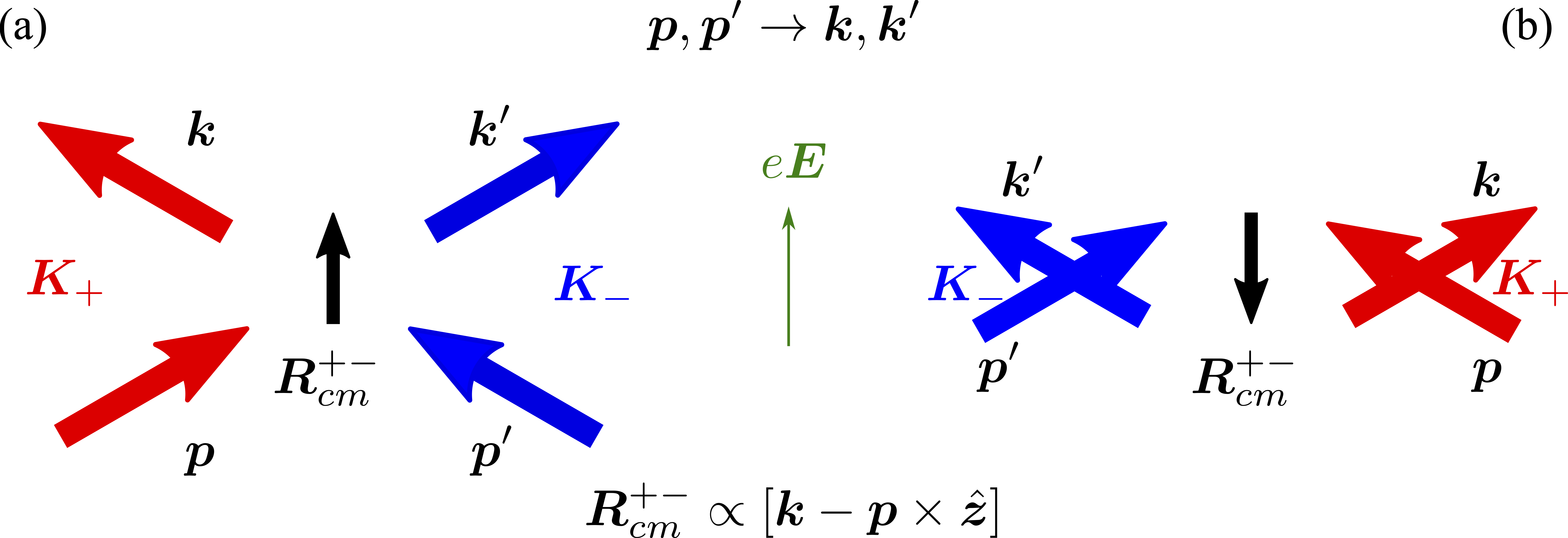
Figure 2: Valley or spin current dissipation and generation at the electron-electron scattering. The process of the electron-electron collision from the initial state $\bm{p},\bm{p}^{\prime}$ to the final state $\bm{k},\bm{k}^{\prime}$ is shown. Thick solid arrows show the electron momenta before and after the collision, color denotes the valleys/spins (red corresponds to the $\bm{K}_{+}$ valley/spin-$\uparrow$ and blue corresponds to the $\bm{K}_{-}$ valley/spin-$\downarrow$). The processes in (a) and (b) differ by the direction of the transferred wavevector $\bm{k}-\bm{p}$ and, accordingly, by the direction of the center of mass shift, $\bm{R}^{+-}_{cm}$, Eq. (45). The collision with positive work of the field ${2}e\bm{E}\cdot\bm{R}^{+-}_{cm}>0$ [panel (a)] reduces the potential energy of the electron pair in the external field and is more efficient than the collision with ${2}e\bm{E}\cdot\bm{R}^{+-}_{cm}<0$ [panel (b)].

To start, let us analyze the role of the skew-scattering and side-jump effects at the electron-electron collisions. To that end, we consider the matrix element of the Coulomb scattering of an electron pair from the states $\bm{k},\bm{k}^{\prime}$ to the states $\bm{p},\bm{p}^{\prime}$. Let $\sigma_{i}$ be the valley index of the $i$th electron, $i=1,2$. The matrix element of the direct scattering process reads Boguslawski (1980); Ş. C. Bădescu et al. (2005); Glazov and Kulakovskii (2009); Badalyan and Vignale (2009)

$$M_{\sigma_{1}\sigma_{2}}(\bm{k},\bm{k}^{\prime}\to\bm{p},\bm{p}^{\prime})=V(q)\delta_{\bm{k}+\bm{k}^{\prime},\bm{p}+\bm{p}^{\prime}}\\ \times\left(1+\mathrm{i}\xi\sigma_{1}[\bm{p}\times\bm{k}]_{z}+\mathrm{i}\xi\sigma_{2}[\bm{p}^{\prime}\times\bm{k}^{\prime}]_{z}\right),$$ (43)

where $V(q)$ is the matrix element of the appropriately screened Coulomb interaction. In Eq. (43) we took into account only $\xi$-linear contributions, see Refs. Glazov and Kulakovskii (2009); Glazov (2010) for the full expression derived in the extended Kane model. The analysis of the skew scattering effect at the electron-electron collisions is presented in Appendix A. It is shown that the skew scattering contribution is absent due to the energy and momentum conservation laws, however, it can result in the valley Hall effect in bilayers, cf. Badalyan and Vignale (2009); Glazov et al. (2011).

It is straightforward to derive, following Refs. Pesin (2018); Chen et al. (2014), the coordinate shifts of the electrons at the Coulomb scattering. In our case the individual shifts of the electronic wavepackages are given by [cf. Eq. (24)]

$$\bm{R}^{\sigma_{1}}_{\bm{p}\bm{k}}=2\xi\sigma_{1}[(\bm{p}-\bm{k})\times\hat{\bm{z}}];\leavevmode\nobreak\ \bm{R}^{\sigma_{2}}_{\bm{p}^{\prime}\bm{k}^{\prime}}=2\xi\sigma_{2}[(\bm{p}^{\prime}-\bm{k}^{\prime})\times\hat{\bm{z}}].$$ (44)

Particularly, for two electrons belonging to the same valley, $\sigma_{1}=\sigma_{2}$, the net shift of the pair, i.e., the shift of their center-of-mass,

$$\bm{R}_{cm}^{\sigma\sigma}=\frac{1}{2}\left(\bm{R}^{\sigma}_{\bm{p}\bm{k}}+\bm{R}^{\sigma}_{\bm{p}^{\prime}\bm{k}^{\prime}}\right)\propto[\bm{p}+\bm{p}^{\prime}-\bm{k}-\bm{k}^{\prime}]\times\hat{\bm{z}}$$

vanishes because of the momentum conservation. Such collisions contribute neither to the net electric current nor to the valley Hall effect. If the electrons are in the opposite valleys, the net shift of the pair can be non-zero, see below. Noteworthy, the side-jump accumulation-induced valley Hall current is contributed by the difference of the shifts for particles at the opposite valleys, $\bm{R}_{diff}=\bm{R}^{\sigma}_{\bm{p}\bm{k}}-\bm{R}^{-\sigma}_{\bm{p}^{\prime}\bm{k}^{\prime}}\propto[\bm{p}+\bm{p}^{\prime}-\bm{k}-\bm{k}^{\prime}]\times\hat{\bm{z}}$, which vanishes because of the momentum conservation.

Importantly, the electron-electron collisions in different valleys (or with opposite spins) result in the side-jump-induced anomalous distribution. It originates from the fact that the electron-electron collisions cause the relaxation of the valley and spin currents Glazov and Ivchenko (2002); D’Amico and Vignale (2002, 2003); Glazov and Ivchenko (2004); Weber et al. (2005). The valley current relaxation is schematically shown in Fig. 2: In the course of collision between electrons in different valleys the $x$-component of the valley current changes despite the total momentum conservation. With account for the electron shifts in the external field the relaxation becomes different for the valley current flowing along the $+x$ and $-x$, cf. panels (a) and (b) of Fig. 2, and valley current can be generated.

To analyze the effect quantitatively, we consider the pair with $\sigma_{1}=+$ and $\sigma_{2}=-$ and calculate the shift of its center of mass at the scattering $\bm{p},\bm{p}^{\prime}\to\bm{k},\bm{k}^{\prime}$ as

$$\bm{R}^{+-}_{cm}=\frac{1}{2}\left(\bm{R}^{+}_{\bm{k}\bm{p}}+\bm{R}^{-}_{\bm{k}^{\prime}\bm{p}^{\prime}}\right)=2\xi[\bm{k}-\bm{p}\times\hat{\bm{z}}].$$ (45)

Taking into account the work of the electric field at the scattering from $\bm{p},\bm{p}^{\prime}\to\bm{k},\bm{k}^{\prime}$ being equal to $2e\bm{E}\cdot\bm{R}^{+-}_{cm}$ we obtain the generation rate of anomalous distribution in the $\bm{K}_{+}$ valley as [cf. Ref. Pesin (2018)]

$$G_{ee,adist}^{+}=\sum_{\bm{p}\bm{p}^{\prime}\bm{k}^{\prime}}\frac{{2}e\bm{E}\cdot\bm{R}^{+-}_{cm}}{k_{B}T}W_{0}(\bm{k},\bm{k}^{\prime};\bm{p},\bm{p}^{\prime})\\ \times f(\varepsilon_{k})f(\varepsilon_{k^{\prime}})[1-f(\varepsilon_{p})][1-f(\varepsilon_{p^{\prime}})],$$ (46)

where $W_{0}(\bm{k},\bm{k}^{\prime};\bm{p},\bm{p}^{\prime})=2|V_{\bm{k}-\bm{p}}|^{2}$ is the symmetric scattering probability, cf. Appendix A. In the $\bm{K}_{-}$ valley the generation rate of the anomalous distribution has the same form as Eq. (46) but the sign is opposite: $G_{ee,adist}^{-}=-G_{ee,adist}^{+}$: Physically the collisions with $e\bm{E}\cdot\bm{R}^{+-}_{cm}>0$ are accompanied by the reduction of the electron pair potential energy [Fig. 2(a)] and are more efficient as compared with the collisions with $e\bm{E}\cdot\bm{R}^{+-}_{cm}<0$ [Fig. 2(b)] where the potential energy of the pair is increased.

In order to find $\Delta f_{\bm{k}}^{\pm,adist:ee}$ we need to determine its relaxation rate. The corresponding electron-electron collision integral reads Glazov and Ivchenko (2002, 2003):

$$Q\{\Delta f^{+},f_{0}\}=\sum_{\bm{p}\bm{p}^{\prime}\bm{k}^{\prime}}W_{0}(\bm{k},\bm{k}^{\prime};\bm{p},\bm{p}^{\prime})\\ \times[\Delta f^{+,ee,adist}_{\bm{k}}F(\bm{k}^{\prime};\bm{p},\bm{p}^{\prime})\\ -\Delta f^{+,ee,adist}_{\bm{p}}F(\bm{p}^{\prime};\bm{k},\bm{k}^{\prime})],$$ (47)

with

$$F(\bm{k}^{\prime};\bm{p},\bm{p}^{\prime})=f^{0}(\varepsilon_{k^{\prime}})[1-f^{0}(\varepsilon_{p})-f^{0}(\varepsilon_{p^{\prime}})]+f^{0}(\varepsilon_{p})f^{0}(\varepsilon_{p^{\prime}}).$$

Comparing Eqs. (46) and (47) we obtain that the generation and dissipation can be balanced provided that

$$\Delta f_{\bm{k}}^{\pm,ee,adist}=\mp{4}\xi e\bm{E}\cdot[\bm{k}\times\hat{\bm{z}}]f_{0}^{\prime}$$ (48)

yielding the bulk valley Hall current (per electron)

$$\bm{v}_{ee,adist}^{\pm}=\frac{{4}\xi e}{\hbar}\hat{\bm{z}}\times\bm{E}.$$ (49)

For further calculations is it convenient to introduce the relaxation time approximation for the electron-electron scattering. In terms of previously introduced generation rates of anomalous distribution this process can be expressed as

$$G_{adist}^{\pm}=\mp\frac{8\xi e}{\hbar}E_{y}N_{1}\frac{\cos{\varphi}}{v\tau_{ee}},$$ (50)

while the electron-electron collision integral can be recast at the same approximation as

$$Q_{ee}\{S_{\varphi}\}=-\frac{S-S_{\varphi}}{\tau_{ee}}.$$ (51)

We abstain from the detailed discussion of the applicability of the relaxation time approximation for the electron-electron collisions in the two-dimensional electron gas with arbitrary degeneracy since typical energy transferred in the collision is $\sim k_{B}T$ and corresponds to the thermal spread of the electron distribution Gantmakher and Levinson (1987); Glazov and Ivchenko (2002, 2004).

III.4 Hydrodynamic regime

Now we have all prerequisites to turn to the hydrodynamic regime of the VHE in ultraclean channels. The electron-electron collisions result in the spin and valley current relaxation. Therefore, in the hydrodynamic regime in the kinetic equation (34) for $S_{\varphi}(x)$, the relaxation times of the first and second angular harmonics are comparable and controlled by the fast electron-electron collisions. It makes purely hydrodynamic description of the valley accumulation inapplicable, in general. Particularly, in the decomposition of $S_{\varphi}(x)$ over the angular harmonics of $\varphi$

$$S_{\varphi}(x)=S_{0}(x)+\cos{\varphi}\,S_{1}(x)+\cos{2\varphi}\,S_{2}(x),$$ (52)

cf. Eq. (8), higher harmonics omitted above are not necessarily small. We make sure, however, that these omitted harmonics are unimportant in our situation due to the specific form of the field-induced $\delta f_{\bm{p}}(x)$, Eq. (12), where the second angular harmonic is already smaller than the first one.

We stress that the simplified kinetic equation (34) is valid at low enough temperatures where $k_{B}T\ll\varepsilon_{F}$ such that the thermal spread of the electron distribution function is practically unimportant. On the other hand, the electron-electron scattering free path $l_{ee}=v\tau_{ee}$ should be smaller than both the mean free path and the channel width:

$$\tau_{ee}\ll\frac{w}{v}\ll\tau.$$

Taking into account that $\tau_{ee}^{-1}=\Lambda(k_{B}T)^{2}/\hbar\varepsilon_{F}$, where $\Lambda\sim 1$ is the dimensionless factor which just slightly depends on the temperature Chaplik (1971); Giuliani and Quinn (1982); Zheng and Das Sarma (1996); Glazov and Ivchenko (2004); Alekseev and Dmitriev (2020), we obtain the following conditions on the system parameters

$$\sqrt{\frac{\hbar v}{l}\varepsilon_{F}}\ll\sqrt{\frac{\hbar v}{w}\varepsilon_{F}}\ll k_{B}T\ll\varepsilon_{F}.$$ (53)

The condition $k_{B}T\ll\varepsilon_{F}$ is, in fact, unessential for the basic physics described below but simplifies the kinetic equation and its solution.

Note that, on the one hand, we neglected impurity scattering within the channel in calculation of the $\delta f_{\bm{p}}(x)$ as in Eq. (12), Sec. II. On the other hand, we account for the impurity scattering to evaluate the side-jump and skew-scattering effects. It is legitimate since the weak scattering gives rise to small corrections to the normal part of the distribution function, but its effect on anomalous transport can be considerable.

Hence, under approximations formulated above, we obtain from Eqs. (34) and (52) the set of equations for the three functions $S_{0,1,2}(x)$:

$$\frac{d}{dx}\left[\frac{v}{2}S_{1}+\left(v_{a}^{+}+v_{sj}^{+}\right)N_{1}\right]=0,$$ (54a)

$$l_{1}\frac{d}{dx}\left(S_{0}+\frac{1}{2}S_{2}\right)+S_{1}=C(x),$$ (54b)

$$\frac{l_{2}}{2}\frac{dS_{1}}{dx}+S_{2}=0.$$ (54c)

Here, as above, the valley relaxation is completely neglected $l_{v}\to\infty$, $l_{1}$ is the relaxation length of the first angular harmonics of the valley distribution, which accounts for the electron-electron collisions, and $l_{2}$ is the relaxation length of the second angular harmonics of the valley distribution function related to the viscosity by Eq. (11). In the simplest possible relaxation time approximation, Eq. (51), $l_{1}=l_{2}=v\tau_{ee}$, but generally $l_{1}$ and $l_{2}$ can be somewhat different. We recall that Eq. (54a) is just a continuity equation for the valley polarization which accounts for the anomalous velocity. The function

$$C(x)=\frac{2l_{1}}{v}\overline{\cos{\varphi}G_{\varphi}^{+}(x)},$$ (55)

in Eq. (54b) describes the generation of the valley Hall current due to the side-jump anomalous distribution and the skew-scattering. We neglected the generation of the second angular harmonics in Eq. (54c) due to the smallness of the second harmonics in the normal distribution function $\delta f_{\bm{p}}$. Equations (54) should be supplemented with the boundary conditions requiring the absence of the valley current at the channels edges:

$$\left.\frac{v}{2}S_{1}+\left(v_{a}^{+}+v_{sj}^{+}\right)N_{1}\right|_{x=\pm w/2}=0.$$ (56)

As a result, the solution of Eq. (54a) takes a particularly simple form

$$S_{1}(x)=-2\frac{v_{a}^{+}+v_{sj}^{+}}{v}N_{1},$$ (57)

which means that the “diffusive” current in the channel compensates the anomalous current, see corresponding analysis for the ballistic case, Eq. (35). Combining Eqs. (54b) and (54c) we obtain the first-order differential equation for the valley population imbalance $S_{0}(x)$ which can be readily solved as

$$S_{0}(x)=\int_{0}^{x}\left[C(x^{\prime})-S_{1}(x^{\prime})+\frac{l_{1}l_{2}}{4}\frac{d^{2}S_{1}(x^{\prime})}{dx^{\prime 2}}\right]\frac{dx^{\prime}}{l_{1}},$$ (58)

where we took into account that $S_{0}(x)$ is an odd function of the coordinate.

Now we present the results for the valley accumulation in the hydrodynamic regime calculated for all relevant mechanisms of the effect after Eq. (58). As in Sec. III.2, we start from the anomalous contributions to the valley accumulation. The anomalous velocity contribution can be readily derived as

$$\Delta N^{\pm,a}(x)=\pm S_{0}(x)=\pm{4}\frac{\xi e}{v\hbar}E_{y}N_{1}\frac{x}{l_{1}}.$$ (59)

This expression has the same form as Eq. (36) with the replacement of $l\to l_{1}\ll l$, resulting in the enhancement of the effect. This is because of the electron-electron interaction which shortens the relaxation time of $S_{1}$: As a result, to compensate the same anomalous current a higher density gradient is needed. The side-jump accumulation effect also results in the contribution to the anomalous velocity which is derived from Eqs. (12) and (30) in the form

$$v_{sj}^{+}(x)=-{\xi\over\hbar}\left(1+{U_{v}\over U_{c}}\right)eE_{y}\frac{v}{2\eta l}\left[\left(\frac{w}{2}\right)^{2}-x^{2}\right].$$ (60)

Note that here $l$ is the mean free path due to the rare electron-impurity collisions. Making use of Eqs. (57) and (58) we arrive at

$$\Delta N^{\pm,sj}(x)=\pm S_{0}(x)=\mp{2\xi e\over v\hbar}\left(1+{U_{v}\over U_{c}}\right)E_{y}N_{1}\frac{x}{l_{1}}\\ \times\frac{v}{2\eta l}\left\{\left[\left(\frac{w}{2}\right)^{2}-\frac{x^{2}}{3}\right]-\frac{l_{1}l_{2}}{2}\right\}.$$ (61)

Provided that the electron-electron collisions control both $l_{1}$ and $l_{2}$, we have $l_{1}l_{2}\ll w^{2}$ and the second term in curly brackets in negligible in the considered hydrodynamic regime. Using the definition of viscosity, Eq. (11), Eq. (61) can be rewritten as

$$\Delta N^{\pm,sj}(x)\\ =\mp\left(1+{U_{v}\over U_{c}}\right){\xi e\over v\hbar}E_{y}N_{1}\frac{x}{l_{1}}\frac{4}{ll_{2}}\left[\left(\frac{w}{2}\right)^{2}-\frac{x^{2}}{3}\right].$$ (62)

The profile of accumulated density thus deviates from the simple linear one, because of the parabolic coordinate dependence of $\delta f_{\bm{p}}(x)$ in the hydrodynamic regime.

Now we turn to the remaining contributions due to the anomalous distribution formed due to the side-jump effect and due to the skew scattering. First we make use of Eqs. (48) and (49) to calculate the profile of the electron density due to the anomalous distribution generated at the electron-electron scattering. Straightforward calculation shows that

$$\Delta N^{\pm,ee,adist}(x)=\mp{8}\frac{\xi e}{v\hbar}E_{y}N_{1}\frac{x}{l_{1}}.$$ (63)

It is twice larger than the contribution due to the anomalous velocity, Eq. (59). Hence, a half of $\Delta N^{\pm,ee,adist}$ compensates $\Delta N^{\pm,a}$. Such compensation, surprising as it may seem, follows directly from comparison of Eqs. (49) and (23). Thus, one half of electron-electron scattering induced anomalous distribution remains

$$\Delta N^{\pm,ee}(x)=\mp{4}\frac{\xi e}{v\hbar}E_{y}N_{1}\frac{x}{l_{1}}.$$ (64)

The anomalous distribution effect due to the impurities can be calculated exactly as in Sec. III.2 with the result

$$\Delta N^{\pm,adist}(x)=\mp\left(1+\frac{U_{v}}{U_{c}}\right)\frac{{2}\xi e}{v\hbar}E_{y}N_{1}\frac{x}{l}.$$ (65)

Note that unlike the anomalous velocity contribution, Eq. (59), here the profile is controlled by the impurity-induced mean free path exactly as in Eq. (39). Finally, for the skew scattering contribution we obtain

$$\Delta N^{\pm,sk}(x)=\\ \pm S_{imp}g\tau\frac{\varepsilon_{F}\tau_{1}}{\hbar}\frac{\xi e}{v\hbar}E_{y}N_{1}\frac{x}{l_{1}}\frac{4}{ll_{2}}\left[\left(\frac{w}{2}\right)^{2}-\frac{x^{2}}{3}\right].$$ (66)

The profile of the valley polarization is the same as for the side-jump accumulation effect. Ratio of the skew-scattering to the side-jump accumulation can be estimated as (at $U_{c}\sim U_{v}$)

$$\left|\frac{gS_{imp}\tau}{1+{U_{v}}/{U_{c}}}\frac{\varepsilon_{F}\tau_{1}}{\hbar}\right|\sim g|U_{c}|\frac{\varepsilon_{F}\tau_{1}}{\hbar},$$

and is a product of small, $g|U_{c}|\ll 1$, and large, $\varepsilon_{F}\tau_{1}/\hbar$, factors. Thus, these contributions can be comparable.

It is worth to note that contribution due to the impurity-induced side-jump accumulation, Eq. (62) and, generally, the contribution caused by the skew scattering, Eq. (66) exceed by far the contribution due to the impurity-induced anomalous distribution, Eq. (65) because $l_{1}l_{2}\ll w$. On the other hand, the remaining contribution from the electron-electron anomalous distribution (with account for compensation of the anomalous velocity), Eq. (64), can be larger or smaller as compared to Eqs. (62) and Eqs. (66) depending on the parameter

$$r=\frac{w^{2}}{ll_{1}},$$ (67)

which is a product of a small $w/l\ll 1$ and large $w/l_{1}\gg 1$ factors. If $r\ll 1$, the contribution due to the electron-electron scattering induced anomalous distribution, Eq. (64), is dominant. On the contrary, if $r\gg 1$, the impurity-induced contributions, Eqs. (62) and (66) dominate. Combining Eqs. (62), (64), and (66) we obtain the leading contribution to the valley polarization in the hydrodynamic regime in the form

$$\Delta N^{\pm,h}(x)=\mp{\xi e\over v\hbar}E_{y}N_{1}\frac{x}{l_{1}}\\ \times\left\{{4}+\left(\mathcal{C}_{sj}+\mathcal{C}_{sk}\right)\frac{4}{ll_{2}}\left[\left(\frac{w}{2}\right)^{2}-\frac{x^{2}}{3}\right]\right\},$$ (68)

with $\mathcal{C}_{sj}=1+U_{v}/U_{c}$ and $\mathcal{C}_{sk}=-S_{imp}g\tau\varepsilon_{F}\tau_{1}/\hbar$. The valley (spin) polarization profile is shown in Fig. 3 by the blue line.

III.5 Discussion

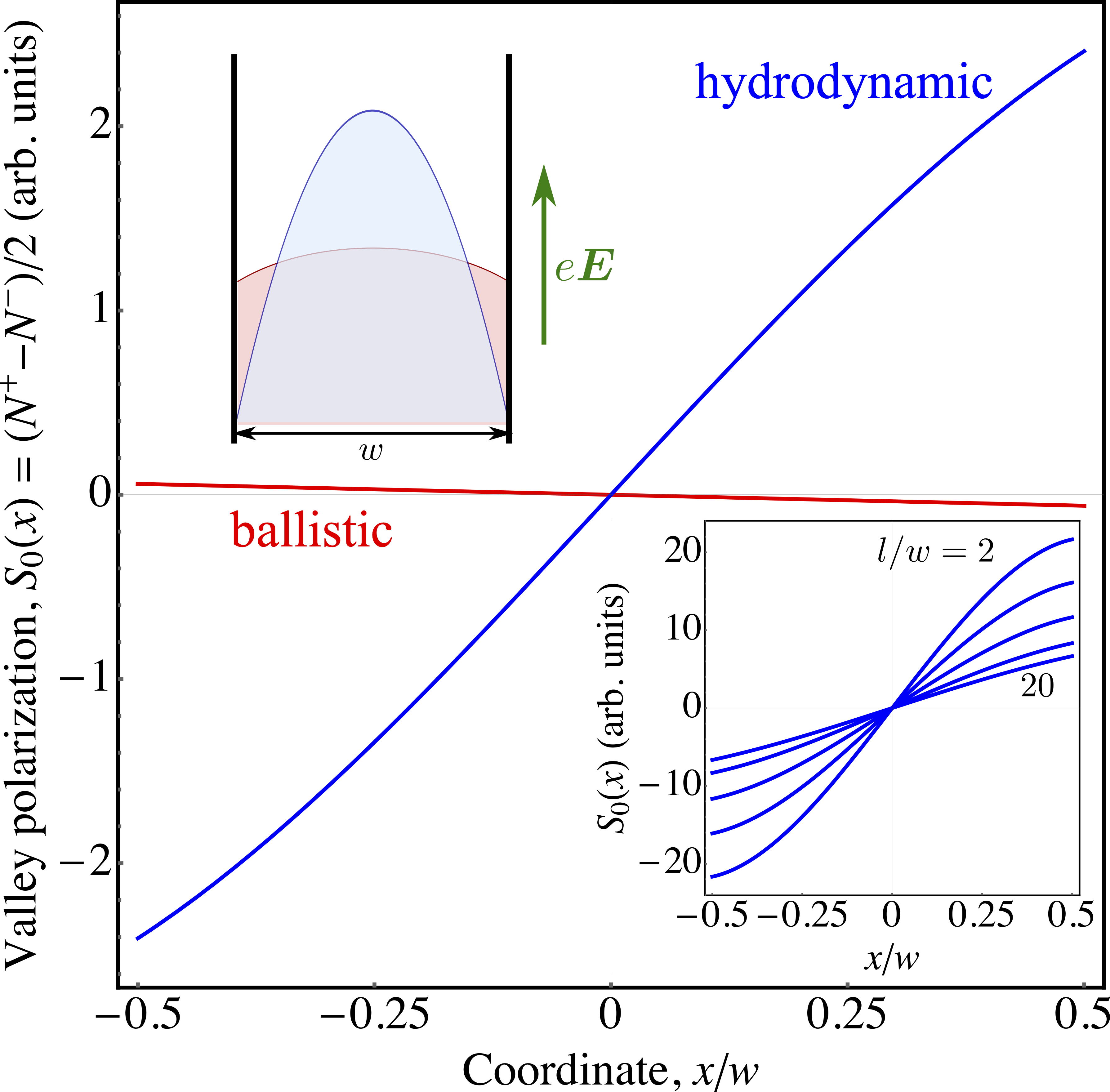
Figure 3: Spin or valley polarization calculated after Eq. (42) (blue line, ballistic channel) and Eq. (68) (red line, hydrodynamic channel). The parameters are $\mathcal{C}_{sj}=1.8$, $C_{sk}=2.2$, and $l/w=5$, $l_{1}=l_{2}=0.3w$. Top left inset shows the schematics of the channel, velocity profiles and direction of the applied field, cf. Fig. 1. Bottom right inset shows the valley polarization in the hydrodynamic channel calculated after Eq. (68) at $\mathcal{C}_{sj}=1.8$, $C_{sk}=2.2$, $l_{1}=l_{2}=0.1w$ and different ratios $l/w=2,3,5,10,20$.

Here we summarize and briefly discuss the obtained results for the valley accumulation within the channel. The valley polarization $S_{0}(x)=[N^{+}(x)-N^{-}(x)]/2$ is plotted in Fig. 3 by the red line for the ballistic regime and blue line for the hydrodynamic regime. In the ballistic regime where the electron-electron scattering is negligible the main contribution to the valley polarization is given by the combination of the anomalous velocity and side-jump induced anomalous distribution effects due to the residual disorder, Eq. (42). Corresponding valley polarization is linear in the coordinate, see the red curve in Fig. 3. By contrast, in the hydrodynamic regime, the anomalous velocity is compensated by the anomalous distribution induced by the electron-electron collisions. The resulting valley polarization is driven by the remaining part of the electron-electron scattering induced anomalous distribution, as well as by the side-jump accumulation and skew scattering due to the residual disorder, Eq. (68). Here the dependence is more complicated, it is linear at $x\ll w$ and saturates near the edge boundaries, blue curve in Fig. 3.

Let us compare the valley polarization magnitude for the ballistic and hydrodynamic channels in more detail. Generally, the distributions of electrons in $\bm{K}_{\pm}$ valleys can be recast in the form

$$N^{+}(x)=-N^{-}(x)=S_{0}(x)=\mathcal{C}\frac{\xi e}{v\hbar}E_{y}N_{1}\mathcal{D}(x),$$ (69)

where the coefficient $\mathcal{C}\sim 1$ depends on the mechanism, the factor $\xi eE_{y}N_{1}/(v\hbar)$ is the same for all mechanisms, and the function $\mathcal{D}(x)$ describes the coordinate distribution:

$$\mathcal{D}(x)=\frac{x}{l}\times\begin{cases}1,\quad\mbox{ball},\\ \frac{1}{l_{1}l_{2}}\left[\left(\frac{w}{2}\right)^{2}-\frac{x^{2}}{3}\right],\quad\frac{w^{2}}{ll_{1}}\gg 1,\quad\mbox{hyd},\\ \frac{l}{l_{1}},\quad\quad\frac{w^{2}}{ll_{1}}\ll 1,\quad\mbox{hyd},\end{cases}$$ (70)

for the leading contributions in the ballistic (bal) and hydrodynamic (hyd) regimes. Importantly, the valley accumulation in the hydrodynamic regime is parametrically larger than in ballistic regime because $l_{1}$, $l_{2}\sim v\tau_{ee}\ll w$. The difference of the signs of the slopes of the accumulated polarization for the ballistic and hydrodynamic channels results from the fact that in the the anomalous velocity dominates in ballistic channel for the parameters of our calculation.

Interestingly, in the hydrodynamic regime the magnitude and shape of the valley polarization depend on the ratio $l/w$ (at fixed $l_{1}/w,l_{2}/w$), see Eqs. (68), (70) and the bottom right inset in Fig. 3. This is because with increase in $l/w$ the role of the impurity scattering within the channel is suppressed. Thus, corresponding side-jump and skew-scattering contributions become less important. These contributions provide non-linear shape of the valley polarization arising from the specific shape of the electron distribution in the Poiseuille flow [Eq. (12)], see the second term in curly brackets of Eq. (68). Hence, in accordance with the bottom right inset in Fig. 3 increase in $l/w$ makes the valley polarization smaller and its coordinate dependence closer to a linear one. Note that for fixed system parameters (mean free paths, $\xi$, $N_{1}$ and $\mathcal{C}_{sj},\mathcal{C}_{sk}$) the valley polarization increases $\propto w$ in the ballistic case or as $w^{3}$ or $w$ in the hydrodynamic case depending on $w^{2}/ll_{1}$, Eq. (70).

IV Valley and spin accumulation in impurity stripes

IV.1 Model

Let us now turn to the valley and spin Hall and accumulation effects in the impurity stripes. Here the spin or valley imbalance has two sources: (i) the VHE or SHE induced by the electric field acting on the electrons within the stripes and (ii) the VHE or SHE resulting from the electrons which were driven by the field in the channel and enter the stripes to loose their momentum. The latter is associated with the $\delta f_{\bm{p}}^{\lessgtr}(x)$ contributions in the distribution function of electrons in the stripe, see Eqs. (14). The contribution (i) can be readily evaluated because the electron motion within the stripe is diffusive. Thus, the anomalous Hall current can be calculated after Ref. Glazov and Golub (2020a) with the result

$$j^{\pm}_{x}=\mp\sigma_{\rm VH}E_{y},$$ (71)

where $\sigma_{\rm VH}$ for all relevant mechanisms is given in the Tab. I of Ref. Glazov and Golub (2020a). Since no current flows through the stripe boundaries the density gradient forms inducing the diffusive current and compensating the valley or spin Hall current. To calculate the distribution function and polarization we use the kinetic Eq. (34) with $Q_{ee}\equiv 0$ and $\tau\to\tau_{i}$:

$$\frac{\partial}{\partial x}\left[v_{x}S_{\varphi}(x)+\left(v_{a}^{+}+v_{sj}^{+}\right)N_{1}\right]+\frac{S_{\varphi}-\overline{S_{\varphi}}}{\tau_{i}}\\ =G^{+}(\varphi,x).$$ (72)

For the polarization distribution caused by the VHE or SHE within the stripe, Eq. (71), we have [cf. Eq. (35)]

$$\Delta N^{\pm}_{i,1}(x)=\frac{2j_{\rm VH}}{evl_{i}}\left(x-\frac{w}{2}\right)=\mp\frac{2\sigma_{\rm VH}}{evl_{i}}\left(x-\frac{w}{2}\right),$$ (73)

for $w/2\leqslant x\leqslant w/2+d$ [right impurity stripe, see Fig. 1(b)]; for the left impurity stripe where $-d-w/2\leqslant x\leqslant-w/2$ the distribution is the same with the replacement of $x-w/2$ by $x+w/2$. We stress that Eq. (73) is derived for the long spin or valley relaxation length in the impurity stripes, $l_{v,i}\gg d$.

We now address the contribution (ii) related to the electrons entering the impurity stripe from the channel. As previously, we use the term valley to denote both the valley and spin degrees of freedom. The contribution to the valley Hall effect and valley accumulation has two origins: the side-jump accumulation and the skew-scattering. Hereafter we consider the right stripe, $w/2\leqslant x\leqslant w/2+d$, for specificity, and the valley polarization in the left stripe can be obtained by the mirror reflection.

We use Eq. (30) to evaluate the velocity due to the side-jump accumulation effect with the result

$$v_{sj}^{\pm}(x)=\pm V_{a}\times\begin{cases}\mathcal{F}_{1}\left(\frac{x-w/2}{l_{i}}\right),\leavevmode\nobreak\ \leavevmode\nobreak\ \mbox{ball},\\ \mathcal{F}_{-1}\left(\frac{x-w/2}{l_{i}}\right),\leavevmode\nobreak\ \mbox{hyd},\end{cases}$$ (74)

where ‘ball’ and ‘hyd’ refers to the ballistic and hydrodynamic regime of the electron propagation within the channel and the corresponding form of $\delta f^{>}_{\bm{p}}(x)$, Eqs. (16a) and (16b), respectively,

$$V_{a}=-\left(1+\frac{U_{v}}{U_{c}}\right)\frac{\xi eE_{y}}{\hbar}\frac{w}{l_{i}}\times\begin{cases}1,\leavevmode\nobreak\ \leavevmode\nobreak\ \mbox{ball},\\ 4,\leavevmode\nobreak\ \leavevmode\nobreak\ \mbox{hyd},\end{cases}$$ (75)

and we introduced the set of functions (their properties are presented in Appendix B)

$$\mathcal{F}_{n}(z)=\int_{-\pi/2}^{\pi/2}\frac{\sin^{2}{\varphi}}{\cos^{n}{\varphi}}\exp(-\frac{z}{\cos{\varphi}})\frac{d\varphi}{\pi},\quad z>0.$$ (76)

One can readily check that $S_{\varphi}(x)$ in the form

$$S^{sj,>}_{\varphi}(x)=-\frac{2V_{a}}{v}N_{1}\sin^{2}\varphi\exp(-\frac{x-w/2}{l_{i}\cos{\varphi}})\\ \times\begin{cases}\cos^{-2}{\varphi},\quad\mbox{ball},\\ 1,\quad\mbox{hyd},\end{cases}$$ (77)

satisfies Eq. (72) with $G^{+}\equiv 0$, $v_{a}^{+}\equiv 0$ and $v_{sj}^{+}$ given by Eq. (74), see Appendix C for details. Particularly, for the accumulated valley distribution we have

$$\Delta N^{\pm,sj}_{i,>}(x)=\pm\overline{S^{sj,>}_{\varphi}(x)}\\ =\mp\frac{V_{a}}{v}N_{1}\begin{cases}\mathcal{F}_{2}\left(\frac{x-w/2}{l_{i}}\right),\quad\mbox{ball},\\ \mathcal{F}_{0}\left(\frac{x-w/2}{l_{i}}\right),\quad\mbox{hyd}.\\ \end{cases}$$ (78)

The generation term due to the skew scattering can be recast in the following form by virtue of Eq. (32)

$$G^{+}(\varphi,x)=\cos{\varphi}\,G_{sk}\begin{cases}\mathcal{F}_{1}\left(\frac{x-w/2}{l_{i}}\right),\quad\mbox{ball},\\ \mathcal{F}_{-1}\left(\frac{x-w/2}{l_{i}}\right),\quad\mbox{hyd}.\end{cases}$$ (79)

where the parameter $G_{sk}$ is given by

$$G_{sk}=\frac{2\xi e}{\hbar}E_{y}N_{1}S_{imp}^{\prime}g\tau_{i}\frac{\varepsilon_{F}\tau_{i}}{\hbar}\frac{w}{l_{i}^{2}}\times\begin{cases}1,\leavevmode\nobreak\ \leavevmode\nobreak\ \mbox{ball},\\ 4,\leavevmode\nobreak\ \leavevmode\nobreak\ \mbox{hyd}.\end{cases}$$ (80)

Note that in Eq. (80) we introduced $S_{imp}^{\prime}$ responsible for the skew scattering by the disorder in the impurity stripe. It has a form similar to Eq. (26) but with the parameters of the impurity stripe:

$$S_{imp}^{\prime}={{2\pi}U_{v}\over\tau_{i}}-\frac{U_{v}}{U_{c}}\frac{\hbar}{g\varepsilon_{F}\tau_{i}^{2}}.$$ (81)

In this situation where $G^{+}\propto\cos{\varphi}$, the solution of Eq. (72) reads [see Appendix C]

$$S^{sj,>}_{\varphi}(x)=-\frac{1}{v\cos{\varphi}}\int_{x}^{\infty}G^{+}(\varphi,x^{\prime})dx^{\prime}.$$ (82)

Accordingly,

$$\Delta N^{\pm,sk}_{i,>}(x)=\pm\overline{S^{sj,>}_{\varphi}(x)}\\ =\mp\frac{G_{sk}l_{i}}{v}\begin{cases}\mathcal{F}_{0}\left(\frac{x-w/2}{l_{i}}\right),\quad\mbox{ball},\\ \mathcal{F}_{-2}\left(\frac{x-w/2}{l_{i}}\right),\quad\mbox{hyd}.\end{cases}$$ (83)

Equations (73), (78), and (83) give the valley accumulation in the right impurity stripe. As already mentioned, the results for the left stripe can be obtained by the mirror reflection.

IV.2 Discussion

Let us analyse the magnitudes of the effects in more detail. To that end we present the valley Hall conductivity $\sigma_{\rm VH}$ in Eqs. (71) and (73) as Glazov and Golub (2020a)

$$\sigma_{\rm VH}=\mathcal{C}_{\rm VH}\frac{\xi e^{2}}{\hbar}\xi N_{1},$$ (84)

where $\mathcal{C}_{\rm VH}$ is the dimensionless coefficient on the order of unity determined by the details of the scattering. As a result, for $\Delta N^{\pm}_{i,1}$ we obtain

$$\Delta N_{i,1}^{\pm}(x)=\mp 2\mathcal{C}_{\rm VH}\frac{\xi e}{v\hbar}E_{y}N_{1}\frac{x-w/2}{l_{i}}.$$ (85)

Naturally, this contribution related to the VHE on the electrons resident in the impurity stripe depends linearly on the coordinate, and its slope is determined by $1/l_{i}$. The contributions due to the electrons entering the stripe, Eqs. (78), and (83), can be combined in the similar form

$$\Delta N_{i,2}^{\pm}(x)=\pm\mathcal{C}^{\prime}\frac{\xi e}{v\hbar}E_{y}N_{1}\frac{w}{l_{i}}\mathcal{F}\left(\frac{x-w/2}{l_{i}}\right).$$ (86)

Here $\mathcal{C}^{\prime}$ is the coefficient (typically, on the order of unity) describing the side-jump accumulation and skew-scattering effects [cf. Eq. (68)] and $\mathcal{F}(x)$ is the appropriate coordinate-dependent function. Since the impurity stripes are short and characterized by small mean free path $l_{i}\ll d\ll w$ the factor $w/l_{i}\gg 1$ in Eq. (86). Therefore the dominant contribution to the valley accumulation in the stripes comes from the electrons entering the stripe from the channel and loose their momentum in the stripe, $|\Delta N_{i,2}^{\pm}(x)|\gg|\Delta N_{i,1}^{\pm}(x)|$.

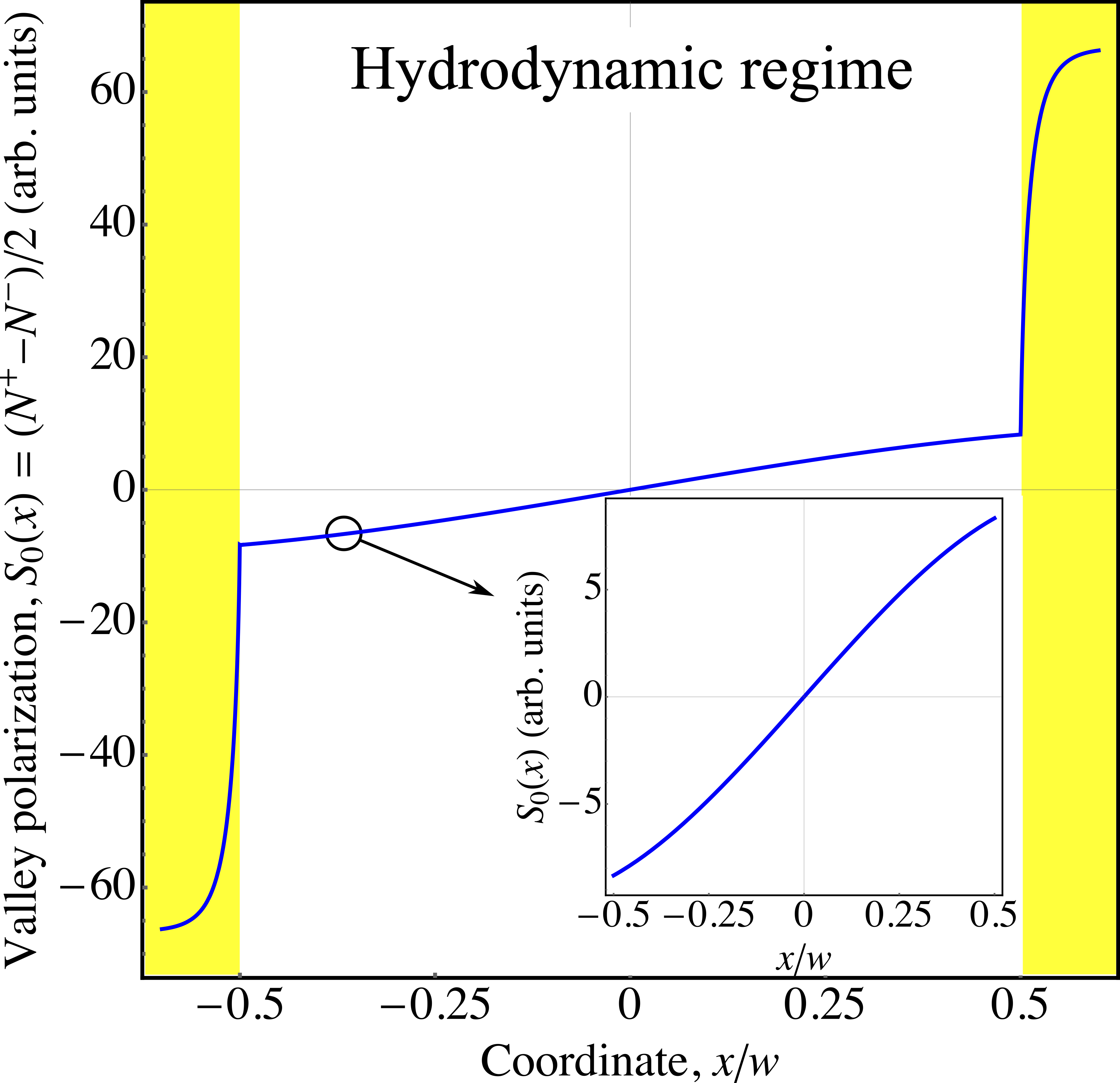
Figure 4: Spin or valley polarization in the ultraclean channel in the hydrodynamic regime calculated after Eq. (68) (inside the channel) and Eq. (78) (in the impurity stripes shown by yellow shaded areas). Shaded areas show the impurity stripes. For the illustrative purposes we took into account only the side-jump contributions. Inset shows the zoom-in of the valley polarization inside the channel, cf. Fig. 3. The parameters are $l/w=10$, $l_{1}=l_{2}=w/10$, $d=w/10$, $l_{i}=d/3$.

We compare now the results for the valley accumulation within the channel and the impurity stripes assuming that the dimensionless coefficients $\mathcal{C}$, $\mathcal{C}^{\prime}$, …are about the same. In the ballistic regime the comparison is straightforward: Making use of Eqs. (69) and (70) we obtain that the valley accumulation in the channel is suppressed by the factor $l_{i}/l$ as compared with the valley accumulation in the impurity stripe. In the hydrodynamic regime the situation is more complex: The profile of the valley polarization within the channel is controlled by the parameter $r$, Eq. (67). The corresponding ratio of the valley density in the channel and in the impurity edge is determined by another ratio

$$R=\begin{cases}\frac{l_{i}}{l}\left(\frac{w}{l_{ee}}\right)^{2},\quad r\gg 1,\\ \frac{l_{i}}{l_{ee}},\quad r\ll 1.\end{cases}$$

This ratio $R$ can, in general, be large or small. For very long impurity-induced mean free path $r\ll 1$ and $R\ll 1$ as well, since in any case $l_{i}\ll l_{ee}$ and the accumulation in the impurity stripes dominates. For moderate mean free paths where $r\gg 1$ the parameter $R\gtrsim 1$ and the valley polarization in the channel can be dominant.

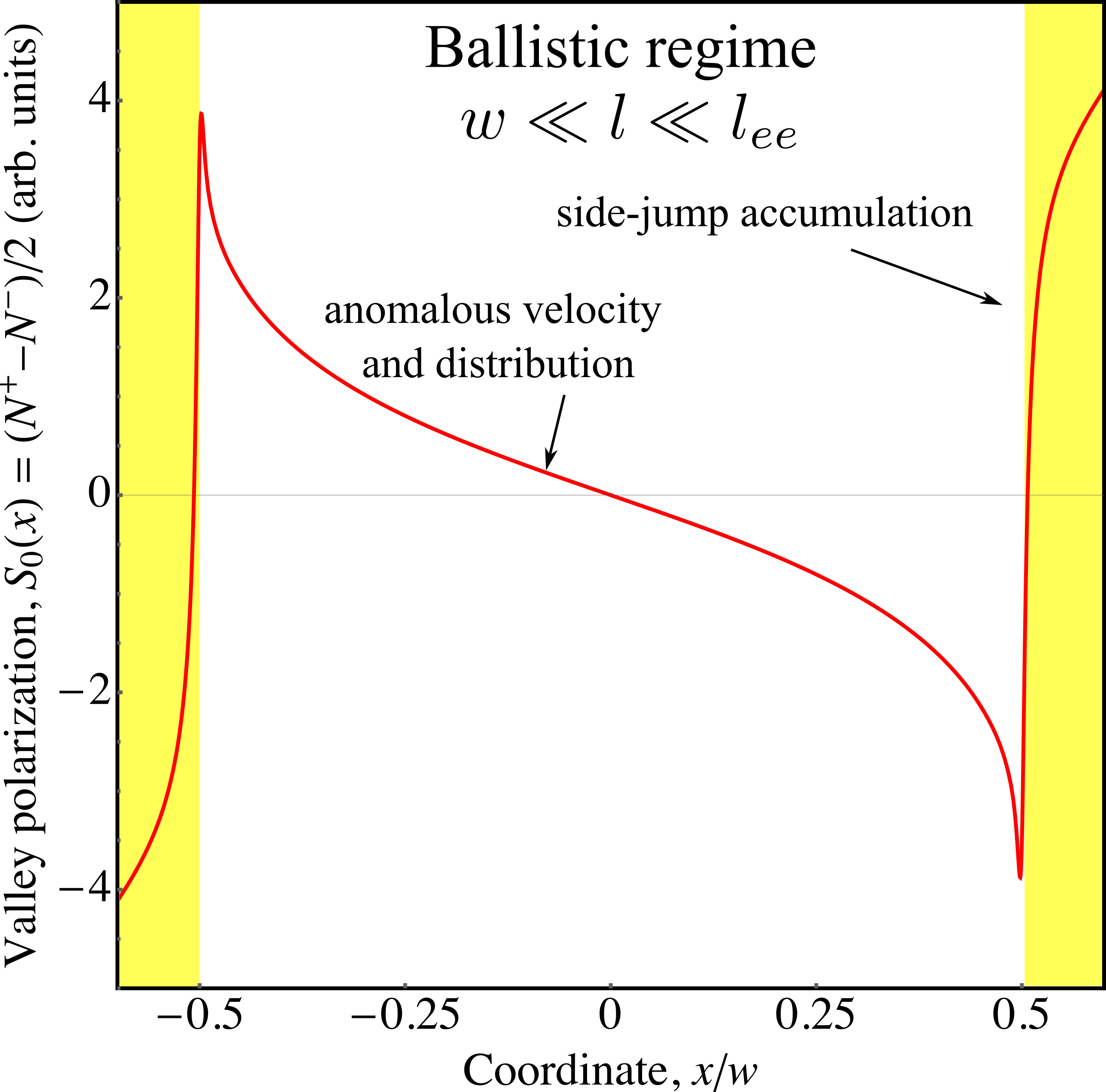
Figure 5: Spin or valley polarization in the ultraclean channel in the ballistic regime calculated after Eq. (105), see Appendix D. For illustrative purposes we disregard skew scattering and take $U_{v}=U_{c}$ which results in the cancellation of the anomalous velocity in the channel. Parameters are $w/l=1/5$, $l_{i}/l=1/10$, the mean free path changes between $l$ and $l_{i}$ at the channel edges on the length $\chi=l/20$. Yellow shaded areas demonstrate impurity stripes.

The dependence of the valley polarization on the coordinate $x$ should be continuous across the whole system “channel+impurity stripes”. Thus, to construct the complete solution the constants should be added to $\Delta N^{\pm}_{>}(x)$ and $\Delta N^{\pm}_{<}(x)$ to match the solutions within the channels and in the impurity stripes. Such a procedure works in the case of hydrodynamic regime where the solutions within the impurity stripe are given by the smooth functions $\mathcal{F}_{0}$ and $\mathcal{F}_{-2}$, see Eqs. (78) and (83) and Appendix B. Corresponding valley polarization shown in Fig. 4 is calculated using Eq. (68) (inside the channel) and Eq. (78) (in the impurity stripes) and matching the valley polarization $S_{0}$ at the channel-stripe boundaries in the hydrodynamic regime. In this case, the parameter $R\ll 1$, and the valley accumulation in the impurity stripes is largest.

In the ballistic regime such simple matching of solutions is impossible: If follows from Eq. (78) that the side-jump contribution diverges at the boundary between the impurity stripe and the channel. Indeed, function $\mathcal{F}_{2}(|x\pm w/2|/l)\propto|x\pm w/2|^{-1}$, Eq. (97a), making it impossible to match the solutions. Partially, this divergence results from using the simplified form of the distribution functions inside the impurity stripes, Eqs. (15a) and (16a). These simplified solutions are inapplicable for $|\cos{\varphi}|\ll w/l$. Replacing the approximate solutions by their exact form, see Eq. (17), we weaken the singularity: For $|x\pm w/2|/l\ll w/l$ function $\mathcal{F}_{2}$ is replaced by $\mathcal{F}_{1}$ which has only logarithmic divergence. Eq (97b). This logarithmic divergence comes from the simplification of our model where the momentum relaxation time abruptly changes between the channel and impurity stripe. This divergence, together with the jump of the side-jump accumulation contribution to the velocity, results in the divergence of the valley occupancy at the edge. To overcome the divergence, we need to take into account that the transition between the channel and impurity stripe is not abrupt, but the scattering time $\tau$ (and the mean free path $l$) continuously changes between $\tau$ and $\tau_{i}$ ($l$ and $l_{i}$) as a function of coordinate. While the detailed analysis of the effects in ballistic channels will be reported elsewhere, we briefly summarize the calculations in Appendix D. The calculated of the valley polarization in the ballistic channel are presented in Fig. 5. One clearly see the pronounced features in the valley polarization arising in the vicinity of the channel edges, confirming our qualitative analysis presented above.

V Summary

We developed the theory of the valley and spin Hall effects and polarization accumulation in the ultraclean channels made from two-dimensional semiconductors where the mean free path of the electron $l$ exceeds by far the channel width $w$. In this case the electron conductivity is controlled by the edge scattering. We considered two regimes of the electron transport: ballistic, where the electrons rarely scatter off residual disorder, and hydrodynamic, where the electron-electron collisions are efficient such that the electron-electron scattering free path $l_{ee}\ll w$. Correspondingly, in the former regime the electrons are practically ballistic, while in the latter regime the electrons can be considered as a viscous fluid.

Under conditions of the valley or spin Hall effect the electric field applied along the channel results in the transversal valley or spin current. The latter gives rise to the gradient of the valley or spin polarization – inhomogeneous polarization accumulation – which compensates the transversal valley current.

We identified the key mechanisms of the polarization accumulation related to the (i) anomalous velocity in the external electric field, (ii) side-jump, and (iii) skew-scattering and analyzed their contributions to the valley and spin accumulation effect. These mechanisms stem from the effective spin-orbit coupling resulting from the mixing of the conduction and valence bands. Generally, all these mechanisms are equally important and manifest themselves at different parts of the channel.

At the ballistic regime, the valley or spin accumulation inside the channel is mainly controlled by the anomalous velocity and side-jump induced anomalous distribution, while the contributions of the side-jump accumulation and skew scattering are smaller by the factor $\sim w/l$.

At the hydrodynamic regime, additional contributions to the effect result from the electron-electron collisions which both provide efficient dissipation of the valley current, and contribute to the side-jump anomalous distribution effect. As a result, the anomalous velocity contribution inside the channel is compensated. We show that the valley or spin accumulation in hydrodynamic channels is controlled by an interplay of the side-jump accumulation and skew scattering by the residual impurities in the channel, as well as by the electron-electron scattering induced anomalous distribution. At the same time, the anomalous distribution effect due to the impurities is suppressed by the factor $w^{2}/l_{ee}^{2}$.

Importantly, the significant accumulation of the valley or spin polarization takes place in the immediate vicinity of the channel edges. The physical reason is related to the fact, that the electron momentum relaxation is provided by the edges. To calculate the valley accumulation near the edge we suggested the impurity stripe model, which assumes that in the narrow stripes near the channels edges the impurity density is so high that the electron transport becomes diffusive. The calculated distribution of the polarization near the edge depends on the transport regime in the channel.

Note that additional contribution to the valley or spin accumulation in the channel may result from the rotational viscosity of the electrons which transforms a curl of the velocity to the valley or spin polarization de2013non ; PhysRevB.96.020401 ; Takahashi:2020um . This effect requires spin or valley relaxation and deserves further studies.

Regarding the observation of spin or valley Hall effect in ultraclean channels, we expect that the effect is easier to observe in conventional GaAs-based Hall bar samples where the mean free path due to the residual disorder exceeds tens of microns. However, the progress in 2D material technology makes us confident that the structures based on transition metal dichalcogenide monolayers with $l\gg w$ will also be available opening up prospects to study ballistic and hydrodynamic transport in such systems.

VI Conclusion

To conclude, the theory of the spin and valley accumulation in ultraclean two-dimensional semiconductor channels is proposed. The theory is considers both ballistic and hydrodynamic regimes of the electron transport and the model takes into account all relevant contributions to the valley and spin Hall effect. We demonstrate that the main contribution to the valley and spin accumulation appear in the vicinity of the channel edges where the momentum relaxation occurs.

Appendix A Skew scattering at the electron-electron collisions

The absence of the skew scattering induced VHE for the collisions of the electrons belonging to the same valley, $\sigma_{1}=\sigma_{2}$, is straightforward to show. Indeed, despite the presence of asymmetric terms in Eq. (43), the valley Hall current cannot be generated because of the momentum conservation law: The transversal to the $y$-axis component of the electron momentum cannot appear due to the electron-electron scattering.

Thus, the case of interest for us is then the electrons are in the opposite valleys. To analyze the effect in this case, we introduce the antisymmetrized states as

$$|\bm{k}+,\bm{k}^{\prime}-\rangle=\frac{1}{2\sqrt{\mathcal{S}}}\left[e^{\mathrm{i}\bm{k}\bm{r}_{1}+\mathrm{i}\bm{k}^{\prime}\bm{r}_{2}}\mathcal{U}_{\bm{k},+}(\bm{r}_{1})\mathcal{U}_{\bm{k}^{\prime},-}(\bm{r}_{2})-e^{{\mathrm{i}\bm{k}\bm{r}_{2}+\mathrm{i}\bm{k}^{\prime}\bm{r}_{1}}}\mathcal{U}_{\bm{k}^{\prime},-}(\bm{r}_{1})\mathcal{U}_{\bm{k},+}(\bm{r}_{2})\right],$$ (87a)

$$|\bm{k}-,\bm{k}^{\prime}+\rangle=\frac{{-1}}{2\sqrt{\mathcal{S}}}\left[e^{\mathrm{i}\bm{k}\bm{r}_{1}+\mathrm{i}\bm{k}^{\prime}\bm{r}_{2}}\mathcal{U}_{\bm{k},-}(\bm{r}_{1})\mathcal{U}_{\bm{k}^{\prime},+}(\bm{r}_{2})-e^{{\mathrm{i}\bm{k}\bm{r}_{2}+\mathrm{i}\bm{k}^{\prime}\bm{r}_{1}}}\mathcal{U}_{\bm{k}^{\prime},+}(\bm{r}_{1})\mathcal{U}_{\bm{k},-}(\bm{r}_{2})\right].$$ (87b)

Here $\mathcal{S}$ is the normalization area, $\pm$ in the brackets denote the valley, $\mathcal{U}_{\bm{k},\sigma}(\bm{r})$ is the corresponding Bloch function, and the overall minus sign in Eq. (87b) is introduced for convenience. Making use of Eq. (43) we derive the matrix elements of the electron-electron scattering

$$M\begin{pmatrix}\bm{p}+,\bm{k}+\\ \bm{p}^{\prime}-,\bm{k}^{\prime}-\end{pmatrix}=\delta_{\bm{k}+\bm{k}^{\prime},\bm{p}+\bm{p}^{\prime}}V(\bm{p}-\bm{k})\{1+\mathrm{i}\xi[\bm{p}\times\bm{k}]_{z}-\mathrm{i}\xi[\bm{p}^{\prime}\times\bm{k}^{\prime}]_{z}\},$$ (88a)

$$M\begin{pmatrix}\bm{p}-,\bm{k}+\\ \bm{p}^{\prime}+,\bm{k}^{\prime}-\end{pmatrix}=\delta_{\bm{k}+\bm{k}^{\prime},\bm{p}+\bm{p}^{\prime}}V(\bm{p}^{\prime}-\bm{k})\{1+\mathrm{i}\xi[\bm{p}^{\prime}\times\bm{k}]_{z}-\mathrm{i}\xi[\bm{p}\times\bm{k}^{\prime}]_{z}\}.$$ (88b)

The asymmetry of the scattering rates appears, similarly to the case of impurities or phonons, beyond the Born approximation. The derivation of the full collision integral is quite involved. Here, for illustrative purposes we consider the non-degenerate electron gas in order to neglect the occupancies of the final and intermediate states and greatly simplify the analysis.

To calculate the in-scattering rate to the state $|\bm{k}+,\bm{k}-\rangle$ we need to take into account that the transitions are possible from both $|\bm{p}+,\bm{p}^{\prime}-\rangle$ and $|\bm{p}-,\bm{p}^{\prime}+\rangle$ states. As an intermediate states one has two possible pairs $|\bm{k}_{1}+,\bm{k}_{1}^{\prime}-\rangle$ or $|\bm{k}_{1}-,\bm{k}_{1}^{\prime}+\rangle$. Following Ref. Sturman (1984) we obtain

$$Q_{|\bm{k}+,\bm{k}-\rangle}^{in}=\sum_{\bm{p},\bm{p}^{\prime},\sigma=\pm}W\begin{pmatrix}\bm{k}+,&\bm{p}\sigma\\ \bm{k}^{\prime}-,&\bm{p}-\sigma\end{pmatrix}f_{\bm{p},\sigma}f_{\bm{p}^{\prime},-\sigma},$$ (89)

where $f_{\bm{p},\sigma}$ is the electron distribution function in the valley $\sigma$, and

$$W\begin{pmatrix}\bm{k}+,&\bm{p}\sigma\\ \bm{k}^{\prime}-,&\bm{p}^{\prime}-\sigma\end{pmatrix}=\frac{2\pi}{\hbar}\delta_{\bm{k}+\bm{k}^{\prime},\bm{p}+\bm{p}^{\prime}}\delta(E_{\bm{k}}+E_{\bm{k}^{\prime}}-E_{\bm{p}}-E_{\bm{p}^{\prime}})\times\\ \left[\left|M\begin{pmatrix}\bm{k}+,&\bm{p}\sigma\\ \bm{k}^{\prime}-,&\bm{p}^{\prime}-\sigma\end{pmatrix}\right|^{2}+{2\pi}\sum_{\bm{k}_{1},\bm{k}_{1}^{\prime},\sigma_{1}}\delta_{\bm{k}+\bm{k}^{\prime},\bm{k}_{1}+\bm{k}_{1}^{\prime}}\delta(E_{\bm{k}}+E_{\bm{k}^{\prime}}-E_{\bm{k}_{1}}-E_{\bm{k}_{1}^{\prime}})\right.\\ \left.\times\imaginary\left\{M\begin{pmatrix}\bm{k}+,&\bm{k}_{1}\sigma_{1}\\ \bm{k}^{\prime}-,&\bm{k}_{1}^{\prime}-\sigma_{1}\end{pmatrix}M\begin{pmatrix}\bm{k}_{1}\sigma_{1},&\bm{p}\sigma\\ \bm{k}_{1}^{\prime}-\sigma_{1},&\bm{p}^{\prime}-\sigma\end{pmatrix}M\begin{pmatrix}\bm{p}\sigma,&\bm{k}+\\ \bm{p}-\sigma,&\bm{k}^{\prime}-\end{pmatrix}\right\}\right].$$ (90)

Analogously, the out-scattering term takes the form

$$Q_{|\bm{k}+,\bm{k}-\rangle}^{out}=\sum_{\bm{p},\bm{p}^{\prime},\sigma=\pm}W\begin{pmatrix}\bm{p}\sigma,&\bm{k}+\\ \bm{p}^{\prime}-\sigma,&\bm{k}^{\prime}-\end{pmatrix}f_{\bm{k},+}f_{\bm{k}^{\prime},-}.$$ (91)

Analysis of Eqs. (88) and (90) demonstrates that

$$W\begin{pmatrix}\bm{k}+,&\bm{p}+\\ \bm{k}^{\prime}-,&\bm{p}^{\prime}-\end{pmatrix}=W_{0}(\bm{k}\bm{k}^{\prime};\bm{p}\bm{p}^{\prime})$$ (92a)

$$+W_{1}(\bm{k}\bm{k}^{\prime};\bm{p}\bm{p}^{\prime})\left\{[\bm{p}\times\bm{k}]_{z}-[\bm{p}^{\prime}\times\bm{k}^{\prime}]_{z}\right\},$$

$$W\begin{pmatrix}\bm{k}+,&\bm{p}-\\ \bm{k}^{\prime}-,&\bm{p}^{\prime}+\end{pmatrix}=W_{0}(\bm{k}\bm{k}^{\prime};\bm{p}^{\prime}\bm{p})$$ (92b)

$$+W_{1}(\bm{k}\bm{k}^{\prime};\bm{p}^{\prime}\bm{p})\left\{[\bm{p}^{\prime}\times\bm{k}]_{z}-[\bm{p}\times\bm{k}^{\prime}]_{z}\right\}.$$

where $W_{0}(\bm{k}\bm{k}^{\prime};\bm{p}^{\prime}\bm{p})$ and $W_{1}(\bm{k}\bm{k}^{\prime};\bm{p}^{\prime}\bm{p})$ are the symmetric functions of the scattering angles. Terms $\propto W_{1}$ describe the skew effect at the electron-electron scattering. Note that the asymmetric sum over $\bm{p},\bm{p}^{\prime}$ in Eq. (91) vanishes and the kinetic equation can be brought to the form

$$\frac{\partial f_{\bm{k}}^{+}}{\partial t}+Q_{\bm{k}}\{f^{+},f^{-}\}=0,$$ (93)

where

$$Q_{\bm{k}}\{f^{+},f^{-}\}=2\sum_{\bm{p}\bm{p}^{\prime}\bm{k}^{\prime}}\frac{2\pi}{\hbar}|V_{\bm{p}-\bm{k}}|^{2}\delta_{\bm{k}+\bm{k}^{\prime},\bm{p}+\bm{p}^{\prime}}\\ \times\delta(E_{\bm{k}}+E_{\bm{k}^{\prime}}-E_{\bm{p}}-E_{\bm{p}^{\prime}})(f_{\bm{k}}^{+}f_{\bm{k}^{\prime}}^{-}-f_{\bm{p}}^{+}f_{\bm{p}^{\prime}}^{-})\\ -2\sum_{\bm{p}\bm{p}^{\prime}\bm{k}^{\prime}}W_{1}(\bm{k}\bm{k}^{\prime};\bm{p}\bm{p}^{\prime})\left\{[\bm{p}\times\bm{k}]_{z}-[\bm{p}^{\prime}\times\bm{k}^{\prime}]_{z}\right\}f_{\bm{p}}^{+}f_{\bm{p}^{\prime}}^{-}.$$ (94)

First lines in Eq. (94) describe standard (symmetric) electron-electron scattering in agreement with Refs. Glazov and Ivchenko (2002); D’Amico and Vignale (2002); Glazov and Ivchenko (2003). Last line in Eq. (94) describes the skew-scattering effect at the electron-electron collisions. One can show, however, that due to the energy and momentum conservation the valley Hall effect is absent, provided that $\bm{f}_{\bm{p}}^{+}=\bm{f}_{\bm{p}}^{-}=f_{0}(E_{\bm{p}})(1+\bm{u}\cdot\bm{p})$ (with $\bm{u}$ being a constant vector, i.e., for the current-carrying distribution). Indeed, in such a case the energy and momentum conservation laws yield $f_{\bm{p}}^{+}f_{\bm{p}^{\prime}}^{-}=f_{\bm{k}}^{+}f_{\bm{k}^{\prime}}^{-}$ and the summation over $\bm{p}$ and $\bm{p}^{\prime}$ in the asymmetric term vanishes.

Appendix B Properties of functions $\mathcal{F}_{n}(z)$

The functions $\mathcal{F}_{n}(z)$ are defined as [cf Eq. (76)]

$$\mathcal{F}_{n}(z)=\int_{-\pi/2}^{\pi/2}\frac{\sin^{2}{\varphi}}{\cos^{n}{\varphi}}\exp(-\frac{z}{\cos{\varphi}})\frac{d\varphi}{\pi},\quad z>0.$$ (95)

For $z>0$ the integral converges because at $\cos{\varphi}\to 0$ the exponent rapidly vanishes.

At $z\to\infty$ the leading contribution to the integral results from $\varphi\to 0$ where the $\cos{\varphi}$ reaches its maximum. As a result it is possible to replace $\exp(-z/\cos{\varphi})$ by $\exp[-z(1+\varphi^{2}/2)]$ and $\sin^{2}{\varphi}/\cos^{n}{\varphi}$ by $\varphi^{2}$. As a result

$$\mathcal{F}_{n}(z)\approx\int_{-\infty}^{\infty}\varphi^{2}\exp[-{z}\left(1+\frac{\varphi^{2}}{2}\right)]\frac{d\varphi}{\pi}\\ =\sqrt{\frac{2}{\pi z^{3}}}e^{-z},\quad z\to\infty.$$ (96)

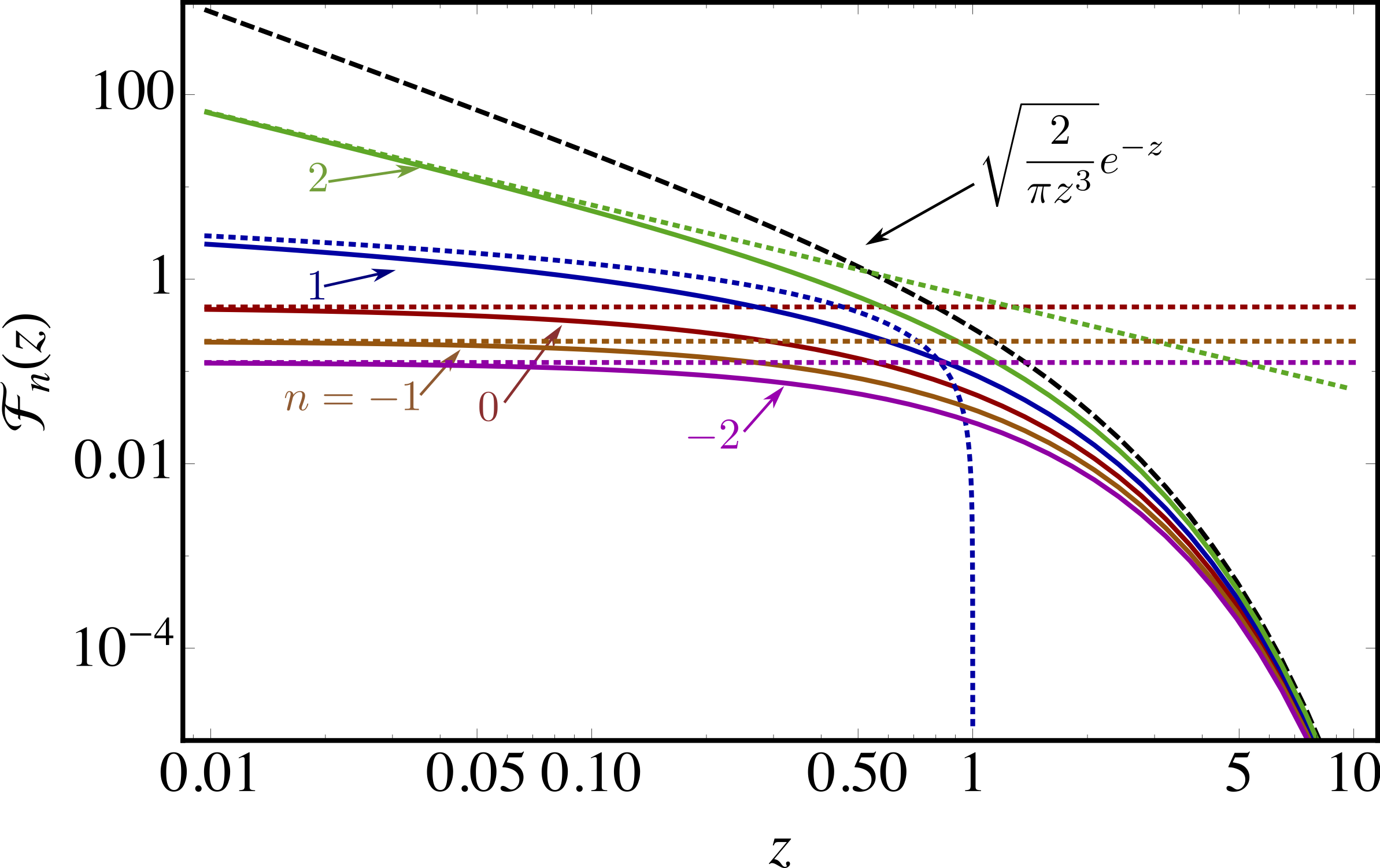
Figure 6: Functions $\mathcal{F}_{n}(z)$ calculated numerically after Eq. (95) (solid lines) and their asymptotics: large-$z$, Eq. (96) (black dashed), and small-$z$, Eqs. (97) (dotted).

At $z\to 0$ for $n>0$ the main contribution to the integral comes from the points where $\cos{\varphi}\to 0$, i.e., at $\varphi\approx\pm\pi/2$. Changing the integration variable and assuming that $\alpha=|\varphi\mp\pi/2|\ll 1$ we have for $n>1$

$$\mathcal{F}_{n}(z)\approx\frac{2}{\pi}\int_{0}^{1}\frac{\exp(-\frac{z}{\alpha})}{\alpha^{n}}d\alpha\\ \approx\frac{2(n-2)!}{\pi z^{n-1}},\quad z\to 0,\leavevmode\nobreak\ \leavevmode\nobreak\ n>1.$$ (97a)

For $$n=1$$ the leading contribution is logarithmic

$$\mathcal{F}_{1}(z)\approx\frac{2}{\pi}\ln{1/z},\quad z\to 0.$$ (97b)

For $$n<0$$ the divergence is absent and

$$\mathcal{F}_{n}(0)=\frac{\Gamma\left[(1-n)/2\right]}{2\sqrt{\pi}\Gamma\left[(2-n)/2\right]},$$ (97c)

where $\Gamma(x)$ is the $\Gamma$-function. The plots of relevant functions $\mathcal{F}_{n}(z)$ for $n=-2,\ldots,2$ are shown in Fig. 6 together with their asymptotics.

Appendix C Solution of kinetic equation in impurity stripes

Here we present the analytical solution of kinetic Eq. (72) describing the valley accumulation in the impurity stripes. We consider the right stripe, $x\geqslant w/2$ for specificity.

First, we address the effect of the anomalous velocity. Let us assume, in agreement with Eq. (74), that

$$v_{a}^{+}(x)=\int_{-\pi/2}^{\pi/2}\Phi(\varphi)\exp(-\frac{x-w/2}{l_{i}\cos{\varphi}})\frac{d\varphi}{\pi},$$ (98)

where $\Phi(\varphi)$ is an arbitrary function of the angle $\varphi$. Let us check that

$$S_{\varphi}(x)=-\frac{2N_{1}}{v\cos{\varphi}}\Phi(\varphi)\exp(-\frac{x-w/2}{l_{i}\cos{\varphi}})\Theta(\cos{\varphi})$$ (99)

satisfies Eq. (72) (with $G^{+}=0$). Indeed,

$$\overline{S_{\varphi}}=-\frac{N_{1}}{v}\int_{-\pi/2}^{\pi/2}\frac{\Phi(\varphi)}{\cos{\varphi}}\exp(-\frac{x-w/2}{l_{i}\cos{\varphi}})\frac{d\varphi}{\pi}\\ =\frac{N_{1}}{\tau_{i}}\frac{\partial v_{a}(x)}{\partial x},$$ (100)

while

$$\frac{\partial}{\partial x}v_{x}S_{\varphi}(x)=\frac{2N_{1}}{l_{i}\cos{\varphi}}\Phi(\varphi)\exp(-\frac{x-w/2}{l_{i}\cos{\varphi}})\Theta(\cos{\varphi})\\ =-\tau_{i}^{-1}S_{\varphi}(x).$$ (101)

Hence

$$\frac{\partial}{\partial x}\left[v_{x}S_{\varphi}(x)+v_{a}^{+}(x)N_{1}\right]=-\frac{1}{\tau_{i}}\left(S_{\varphi}(x)-\overline{S_{\varphi}(x)}\right)$$

and Eq. (72) is fulfilled.

Second, we consider the effect of the generation. In accordance with Eq. (79) we take $G^{+}(\varphi,x)=\cos{\varphi}\mathcal{G}(x)$ with $\mathcal{G}(x)$ being an arbitrary function of coordinate. We take $S_{\varphi}(x)$ to be $\varphi$-independent, as a result the cosine terms in Eq.  (72) cancel and we have

$$v\frac{\partial S_{\varphi}}{\partial x}=\mathcal{G}(x),$$

which yields Eq. (82) of the main text.

The solutions obtained above vanish at $x\to\infty$ (for the right stripe). Corresponding solutions for $x\to-\infty$ can be obtained by the mirror symmetry. To obtain the solution in the whole system one has to add arbitrary constants to $S_{0}(x)=\overline{S_{\varphi}(x)}$ in order to make $S_{0}(x)$ continuous at $x=\pm w/2$.

Appendix D Valley accumulation for arbitrary $l(x)$

Our goal is to solve the kinetic equation for the valley accumulation in the channel with arbitrary dependence of the impurity induced mean free path $l(x)$ [cf. Eqs. (34) and (72)]:

$$\frac{\partial}{\partial x}\left[\cos{\varphi}S_{\varphi}(x)+V_{a}(x)\right]+\frac{S_{\varphi}-\overline{S_{\varphi}}}{l(x)}=g(\varphi,x),$$ (102)

and determine the profile of the valley polarization $\overline{S}_{\varphi}(x)$. Here $V_{a}(x)=N_{1}[v_{a}^{+}+v_{sj}^{+}(x)]/v$ and $g(\varphi,x)=G^{+}(\varphi,x)/v$ are the reduced anomalous velocity and generation rate, respectively. The electron-electron collisions are neglected. To solve Eq. (102) for arbitrary $l(x)$, $V_{a}(x)$ and $g(x)$ it is convenient to pass to the new variable $y$ defined by

$$\frac{dy}{dx}=\frac{1}{l(x)},\quad y(x)=\int_{0}^{x}\frac{dx^{\prime}}{l(x^{\prime})}.$$ (103)

In this case the dependence of $l(x)$ vanishes. Next, we pass from Eq. (102) to the integral equation for $S_{0}(y)\equiv\overline{S_{\varphi}(y)}$ as

$$S_{0}(y)-\int_{-\infty}^{\infty}S_{0}(y_{1})Q(y-y_{1})dy_{1}=R(y),$$ (104)

where the kernel

$$Q(y)=\int_{-\pi/2}^{\pi/2}\frac{\exp(-\frac{|y|}{\cos{\varphi}})}{\cos{\varphi}}=\frac{1}{\pi}K_{0}(|y|),$$

with $K_{0}(y)$ being the modified Bessel function, and

$$R(y)=\int_{-\infty}^{\infty}\left[-\frac{dV_{a}}{dy}+g(\varphi,y)\right]Q(y-y_{1})dy_{1}.$$

Equation (104) can be solved by the Fourier transform

$$S_{0}(y)=\int_{-\infty}^{\infty}\frac{d\xi}{2\pi}e^{\mathrm{i}\xi y}S(\xi),\leavevmode\nobreak\ \leavevmode\nobreak\ S(\xi)=\frac{R(\xi)}{1-\frac{1}{\sqrt{1+\xi^{2}}}},$$ (105)

where $R(\xi)=\int_{-\infty}^{\infty}R(y)\exp(-\mathrm{i}\xi y)$.

References

- Dyakonov (2017) M. I. Dyakonov, ed., Spin physics in semiconductors, 2nd ed., Springer Series in Solid-State Sciences 157 (Springer International Publishing, 2017).
- Dyakonov and Perel’ (1971a) M. I. Dyakonov and V. I. Perel’, “Current induced spin orientation of electrons in semiconductors,” Phys. Lett. A 35A, 459 (1971a).
- Dyakonov and Perel’ (1971b) M.I. Dyakonov and V.I Perel’, “Possibility of Orienting Electron Spins with Current,” JETP Lett. 13, 657 (1971b).
- Hirsch (1999) J. E. Hirsch, “Spin Hall effect,” Phys. Rev. Lett. 83, 1834 (1999).
- Murakami et al. (2003) Shuichi Murakami, Naoto Nagaosa, and Shou-Cheng Zhang, “Dissipationless quantum spin current at room temperature,” Science 301, 1348 (2003).
- Sinova et al. (2004) Jairo Sinova, Dimitrie Culcer, Q. Niu, N. A. Sinitsyn, T. Jungwirth, and A. H. MacDonald, “Universal intrinsic spin Hall effect,” Phys. Rev. Lett. 92, 126603 (2004).
- Wunderlich et al. (2005) J. Wunderlich, B. Kaestner, J. Sinova, and T. Jungwirth, “Experimental observation of the spin-Hall effect in a two-dimensional spin-orbit coupled semiconductor system,” Phys. Rev. Lett. 94, 47204 (2005).
- Kavokin et al. (2005) Alexey Kavokin, Guillaume Malpuech, and Mikhail Glazov, “Optical Spin Hall Effect,” Phys. Rev. Lett. 95, 136601 (2005).
- Leyder et al. (2007) C. Leyder, M. Romanelli, J. Ph. Karr, E. Giacobino, T. C. H. Liew, M. M. Glazov, A. V. Kavokin, G. Malpuech, and A. Bramati, “Observation of the optical spin Hall effect,” Nat Phys 3, 628–631 (2007).
- Mak et al. (2014) K. F. Mak, K. L. McGill, J. Park, and P. L. McEuen, “The valley Hall effect in MoS2 transistors,” Science 344, 1489–1492 (2014).
- Ubrig et al. (2017) Nicolas Ubrig, Sanghyun Jo, Marc Philippi, Davide Costanzo, Helmuth Berger, Alexey B. Kuzmenko, and Alberto F. Morpurgo, “Microscopic Origin of the Valley Hall Effect in Transition Metal Dichalcogenides Revealed by Wavelength-Dependent Mapping,” Nano Letters 17, 5719–5725 (2017).
- Lundt et al. (2019) Nils Lundt, Łukasz Dusanowski, Evgeny Sedov, Petr Stepanov, Mikhail M. Glazov, Sebastian Klembt, Martin Klaas, Johannes Beierlein, Ying Qin, Sefaattin Tongay, Maxime Richard, Alexey V. Kavokin, Sven Höfling, and Christian Schneider, “Optical valley Hall effect for highly valley-coherent exciton-polaritons in an atomically thin semiconductor,” Nature Nanotechnology 14, 770–775 (2019).
- Hall (1881) E. H. Hall, “XXXVIII. On the new action of magnetism on a permanent electric current,” The London, Edinburgh, and Dublin Philosophical Magazine and Journal of Science 5, 157 (1881).
- Nagaosa et al. (2010) Naoto Nagaosa, Jairo Sinova, Shigeki Onoda, A. H. MacDonald, and N. P. Ong, “Anomalous Hall effect,” Rev. Mod. Phys. 82, 1539–1592 (2010).
- Mak et al. (2010) Kin Fai Mak, Changgu Lee, James Hone, Jie Shan, and Tony F. Heinz, “Atomically thin MoS2: A new direct-gap semiconductor,” Phys. Rev. Lett. 105, 136805 (2010).
- Splendiani et al. (2010) Andrea Splendiani, Liang Sun, Yuanbo Zhang, Tianshu Li, Jonghwan Kim, Chi-Yung Chim, Giulia Galli, and Feng Wang, “Emerging photoluminescence in monolayer MoS2,” Nano Letters 10, 1271 (2010).
- Kormanyos et al. (2015) Andor Kormanyos, Guido Burkard, Martin Gmitra, Jaroslav Fabian, Viktor Zólyomi, Neil D Drummond, and Vladimir Fal’ko, “ theory for two-dimensional transition metal dichalcogenide semiconductors,” 2D Materials 2, 022001 (2015).
- Kolobov and Tominaga (2016) Alexander V. Kolobov and Junji Tominaga, Two-Dimensional Transition-Metal Dichalcogenides (Springer International Publishing, 2016).
- Wang et al. (2018) Gang Wang, Alexey Chernikov, Mikhail M. Glazov, Tony F. Heinz, Xavier Marie, Thierry Amand, and Bernhard Urbaszek, “Colloquium: Excitons in atomically thin transition metal dichalcogenides,” Rev. Mod. Phys. 90, 021001 (2018).
- Xiao et al. (2012) Di Xiao, Gui-Bin Liu, Wanxiang Feng, Xiaodong Xu, and Wang Yao, “Coupled spin and valley physics in monolayers of MoS2 and other group-VI dichalcogenides,” Phys. Rev. Lett. 108, 196802 (2012).
- Mak et al. (2012) Kin Fai Mak, Keliang He, Jie Shan, and Tony F. Heinz, “Control of valley polarization in monolayer MoS2 by optical helicity,” Nat Nano 7, 494–498 (2012).
- Xu et al. (2014) Xiaodong Xu, Wang Yao, Di Xiao, and Tony F. Heinz, “Spin and pseudospins in layered transition metal dichalcogenides,” Nat Phys 10, 343–350 (2014).
- Konabe and Yamamoto (2014) Satoru Konabe and Takahiro Yamamoto, “Valley photothermoelectric effects in transition-metal dichalcogenides,” Phys. Rev. B 90, 075430 (2014).
- Jin et al. (2018) Chenhao Jin, Jonghwan Kim, M. Iqbal Bakti Utama, Emma C. Regan, Hans Kleemann, Hui Cai, Yuxia Shen, Matthew James Shinner, Arjun Sengupta, Kenji Watanabe, Takashi Taniguchi, Sefaattin Tongay, Alex Zettl, and Feng Wang, “Imaging of pure spin-valley diffusion current in WS2-WSe2 heterostructures,” Science 360, 893–896 (2018).
- Onga et al. (2017) Masaru Onga, Yijin Zhang, Toshiya Ideue, and Yoshihiro Iwasa, “Exciton Hall effect in monolayer MoS2,” Nature Materials 16, 1193 (2017).
- Unuchek et al. (2019) Dmitrii Unuchek, Alberto Ciarrocchi, Ahmet Avsar, Zhe Sun, Kenji Watanabe, Takashi Taniguchi, and Andras Kis, “Valley-polarized exciton currents in a van der Waals heterostructure,” Nature Nanotechnology 14, 1104 (2019).
- Kulig et al. (2018) Marvin Kulig, Jonas Zipfel, Philipp Nagler, Sofia Blanter, Christian Schüller, Tobias Korn, Nicola Paradiso, Mikhail M. Glazov, and Alexey Chernikov, “Exciton diffusion and halo effects in monolayer semiconductors,” Phys. Rev. Lett. 120, 207401 (2018).
- Kalameitsev et al. (2019) A. V. Kalameitsev, V. M. Kovalev, and I. G. Savenko, “Valley acoustoelectric effect,” Phys. Rev. Lett. 122, 256801 (2019).
- Glazov and Golub (2020a) M. M. Glazov and L. E. Golub, “Valley Hall effect caused by the phonon and photon drag,” Phys. Rev. B 102, 155302 (2020a).
- Glazov and Golub (2020b) M. M. Glazov and L. E. Golub, “Skew Scattering and Side Jump Drive Exciton Valley Hall Effect in Two-Dimensional Crystals,” Physical Review Letters 125, 157403 (2020b).
- Xiao et al. (2010) Di Xiao, Ming-Che Chang, and Qian Niu, “Berry phase effects on electronic properties,” Rev. Mod. Phys. 82, 1959–2007 (2010).
- Kuga et al. (2008) Shun-ichi Kuga, Shuichi Murakami, and Naoto Nagaosa, “Spin Hall effect of excitons,” Phys. Rev. B 78, 205201 (2008).
- Yao and Niu (2008) Wang Yao and Qian Niu, “Berry phase effect on the exciton transport and on the exciton Bose-Einstein condensate,” Phys. Rev. Lett. 101, 106401 (2008).
- Li et al. (2015) Yun-Mei Li, Jian Li, Li-Kun Shi, Dong Zhang, Wen Yang, and Kai Chang, “Light-Induced Exciton Spin Hall Effect in van der Waals Heterostructures,” Phys. Rev. Lett. 115, 166804 (2015).
- Kovalev and Savenko (2019) V. M. Kovalev and I. G. Savenko, “Quantum anomalous valley Hall effect for bosons,” Phys. Rev. B 100, 121405 (2019).
- Gianfrate et al. (2020) A. Gianfrate, O. Bleu, L. Dominici, V. Ardizzone, M. De Giorgi, D. Ballarini, G. Lerario, K. W. West, L. N. Pfeiffer, D. D. Solnyshkov, D. Sanvitto, and G. Malpuech, “Measurement of the quantum geometric tensor and of the anomalous Hall drift,” Nature 578, 381–385 (2020).
- Sinitsyn et al. (2007) N. A. Sinitsyn, A. H. MacDonald, T. Jungwirth, V. K. Dugaev, and Jairo Sinova, “Anomalous Hall effect in a two-dimensional Dirac band: The link between the Kubo-Streda formula and the semiclassical Boltzmann equation approach,” Phys. Rev. B 75, 045315 (2007).
- Sinitsyn (2007) N. A. Sinitsyn, “Semiclassical theories of the anomalous Hall effect,” Journal of Physics: Condensed Matter 20, 023201 (2007).
- Ado et al. (2015) I. A. Ado, I. A. Dmitriev, P. M. Ostrovsky, and M. Titov, “Anomalous Hall effect with massive Dirac fermions,” EPL 111, 37004 (2015).
- de Jong and Molenkamp (1995) M. J. M. de Jong and L. W. Molenkamp, “Hydrodynamic electron flow in high-mobility wires,” Phys. Rev. B 51, 13389–13402 (1995).
- Titov et al. (2013) M. Titov, R. V. Gorbachev, B. N. Narozhny, T. Tudorovskiy, M. Schütt, P. M. Ostrovsky, I. V. Gornyi, A. D. Mirlin, M. I. Katsnelson, K. S. Novoselov, A. K. Geim, and L. A. Ponomarenko, “Giant magnetodrag in graphene at charge neutrality,” Phys. Rev. Lett. 111, 166601 (2013).
- Bandurin et al. (2016) D. A. Bandurin, I. Torre, R. Krishna Kumar, M. Ben Shalom, A. Tomadin, A. Principi, G. H. Auton, E. Khestanova, K. S. Novoselov, I. V. Grigorieva, L. A. Ponomarenko, A. K. Geim, and M. Polini, “Negative local resistance caused by viscous electron backflow in graphene,” Science 351, 1055–1058 (2016).
- Moll et al. (2016) Philip J. W. Moll, Pallavi Kushwaha, Nabhanila Nandi, Burkhard Schmidt, and Andrew P. Mackenzie, “Evidence for hydrodynamic electron flow in PdCoO2,” Science 351, 1061–1064 (2016).
- Gusev et al. (2018) G. M. Gusev, A. D. Levin, E. V. Levinson, and A. K. Bakarov, “Viscous electron flow in mesoscopic two-dimensional electron gas,” AIP Advances 8, 025318 (2018).
- Krishna Kumar et al. (2017) R. Krishna Kumar, D. A. Bandurin, F. M. D. Pellegrino, Y. Cao, A. Principi, H. Guo, G. H. Auton, M. Ben Shalom, L. A. Ponomarenko, G. Falkovich, K. Watanabe, T. Taniguchi, I. V. Grigorieva, L. S. Levitov, M. Polini, and A. K. Geim, “Superballistic flow of viscous electron fluid through graphene constrictions,” Nature Physics 13, 1182–1185 (2017).
- Ku et al. (2020) Mark J. H. Ku, Tony X. Zhou, Qing Li, Young J. Shin, Jing K. Shi, Claire Burch, Laurel E. Anderson, Andrew T. Pierce, Yonglong Xie, Assaf Hamo, Uri Vool, Huiliang Zhang, Francesco Casola, Takashi Taniguchi, Kenji Watanabe, Michael M. Fogler, Philip Kim, Amir Yacoby, and Ronald L. Walsworth, “Imaging viscous flow of the Dirac fluid in graphene,” Nature 583, 537–541 (2020).
- Sulpizio et al. (2019) Joseph A. Sulpizio, Lior Ella, Asaf Rozen, John Birkbeck, David J. Perello, Debarghya Dutta, Moshe Ben-Shalom, Takashi Taniguchi, Kenji Watanabe, Tobias Holder, Raquel Queiroz, Alessandro Principi, Ady Stern, Thomas Scaffidi, Andre K. Geim, and Shahal Ilani, “Visualizing Poiseuille flow of hydrodynamic electrons,” Nature 576, 75–79 (2019).
- Berdyugin et al. (2019) A. I. Berdyugin, S. G. Xu, F. M. D. Pellegrino, R. Krishna Kumar, A. Principi, I. Torre, M. Ben Shalom, T. Taniguchi, K. Watanabe, I. V. Grigorieva, M. Polini, A. K. Geim, and D. A. Bandurin, “Measuring Hall viscosity of graphene’s electron fluid,” Science 364, 162–165 (2019).
- Gusev et al. (2020) G. M. Gusev, A. S. Jaroshevich, A. D. Levin, Z. D. Kvon, and A. K. Bakarov, “Stokes flow around an obstacle in viscous two-dimensional electron liquid,” Scientific Reports 10, 7860 (2020).
- Gurzhi (1963) R. N. Gurzhi, “Minimum of resistance in impurity-free conductors,” JETP 17, 521 (1963).
- Gurzhi (1968) R. N. Gurzhi, “Hydrodynamic effects in solids at low temperatures,” Soviet Physics Uspekhi 11, 255–270 (1968).
- Müller et al. (2009) Markus Müller, Jörg Schmalian, and Lars Fritz, “Graphene: A nearly perfect fluid,” Phys. Rev. Lett. 103, 025301 (2009).
- Andreev et al. (2011) A. V. Andreev, Steven A. Kivelson, and B. Spivak, “Hydrodynamic description of transport in strongly correlated electron systems,” Phys. Rev. Lett. 106, 256804 (2011).
- Torre et al. (2015) Iacopo Torre, Andrea Tomadin, Andre K. Geim, and Marco Polini, “Nonlocal transport and the hydrodynamic shear viscosity in graphene,” Phys. Rev. B 92, 165433 (2015).
- Pellegrino et al. (2017) Francesco M. D. Pellegrino, Iacopo Torre, and Marco Polini, “Nonlocal transport and the hall viscosity of two-dimensional hydrodynamic electron liquids,” Phys. Rev. B 96, 195401 (2017).
- Narozhny et al. (2015) B. N. Narozhny, I. V. Gornyi, M. Titov, M. Schütt, and A. D. Mirlin, “Hydrodynamics in graphene: Linear-response transport,” Phys. Rev. B 91, 035414 (2015).
- Alekseev (2016) P. S. Alekseev, “Negative magnetoresistance in viscous flow of two-dimensional electrons,” Phys. Rev. Lett. 117, 166601 (2016).
- Levitov and Falkovich (2016) Leonid Levitov and Gregory Falkovich, “Electron viscosity, current vortices and negative nonlocal resistance in graphene,” Nature Physics 12, 672–676 (2016).
- Kashuba et al. (2018) Oleksiy Kashuba, Björn Trauzettel, and Laurens W. Molenkamp, “Relativistic Gurzhi effect in channels of Dirac materials,” Phys. Rev. B 97, 205129 (2018).
- Lucas (2017) Andrew Lucas, “Stokes paradox in electronic Fermi liquids,” Phys. Rev. B 95, 115425 (2017).
- Narozhny et al. (2017) Boris N. Narozhny, Igor V. Gornyi, Alexander D. Mirlin, and Jörg Schmalian, “Hydrodynamic approach to electronic transport in graphene,” Annalen der Physik 529, 1700043 (2017).
- Lucas and Fong (2018) Andrew Lucas and Kin Chung Fong, “Hydrodynamics of electrons in graphene,” Journal of Physics: Condensed Matter 30, 053001 (2018).
- Alekseev et al. (2018) P. S. Alekseev, A. P. Dmitriev, I. V. Gornyi, V. Yu. Kachorovskii, B. N. Narozhny, and M. Titov, “Nonmonotonic magnetoresistance of a two-dimensional viscous electron-hole fluid in a confined geometry,” Phys. Rev. B 97, 085109 (2018).
- Alekseev and Semina (2018) P. S. Alekseev and M. A. Semina, “Ballistic flow of two-dimensional interacting electrons,” Phys. Rev. B 98, 165412 (2018).
- Alekseev and Semina (2019) P. S. Alekseev and M. A. Semina, “Hall effect in a ballistic flow of two-dimensional interacting particles,” Phys. Rev. B 100, 125419 (2019).
- Apostolov et al. (2019) S. S. Apostolov, D. A. Pesin, and A. Levchenko, “Magnetodrag in the hydrodynamic regime: Effects of magnetoplasmon resonance and Hall viscosity,” Phys. Rev. B 100, 115401 (2019).
- Hasdeo et al. (2021) Eddwi H. Hasdeo, Johan Ekström, Edvin G. Idrisov, and Thomas L. Schmidt, “Electron hydrodynamics of two-dimensional anomalous Hall materials,” Phys. Rev. B 103, 125106 (2021).
- Funaki et al. (2021) Hiroshi Funaki, Riki Toshio, and Gen Tatara, “Vorticity-induced anomalous Hall effect in electron fluid,” preprint arXiv:2103.00861 (2021)
- (69) Gen Tatara, Hydrodynamic theory of vorticity-induced spin transport, Phys. Rev. B 104, 184414 (2021). .
- Fuchs (1938) K. Fuchs, “The conductivity of thin metallic films according to the electron theory of metals,” Mathematical Proceedings of the Cambridge Philosophical Society, 34, 100–108 (1938).
- Reuter and Sondheimer (1948) G.E.H. Reuter and E.H. Sondheimer, “The theory of the anomalous skin effect in metals,” Proc. Roy. Soc. A 195, 336 (1948).
- Fal’kovskii (1970) L. A. Fal’kovskii, “Diffuse Boundary Condition for Conduction Electrons,” JETP Lett. 11, 138 (1970).
- (73) L.D. Landau and E.M. Lifshitz, Physical Kinetics, (Butterworth-Heinemann, Oxford, 1981).
- Greene (1966) R. F. Greene, “Boundary conditions for electron distributions at crystal surfaces,” Phys. Rev. 141, 687–689 (1966).
- Andreev (1972) A. F. Andreev, “Interaction of conduction electrons with a metal surface,” Sov. Phys.-Uspekhi, 14, 609–615 (1972).
- Kiselev and Schmalian (2019) Egor I. Kiselev and Jörg Schmalian, “Boundary conditions of viscous electron flow,” Phys. Rev. B 99, 035430 (2019).
- (77) E. L. Ivchenko, Optical spectroscopy of semiconductor nanostructures, (Alpha Science, Harrow UK, 2005).
- (78) L. D. Landau and E. M. Lifshitz, Quantum Mechanics: Non-Relativistic Theory, (Butterworth-Heinemann, Oxford, 1977).
- (79) J. Davies, The physics of low-dimensional semiconductors. (Cambridge University Press, 1998).
- Karplus and Luttinger (1954) Robert Karplus and J. M. Luttinger, “Hall effect in ferromagnetics,” Phys. Rev. 95, 1154–1160 (1954).
- Belinicher et al. (1982) V. I. Belinicher, E. L. Ivchenko, and B. I. Sturman, “Kinetic theory of the displacement photovoltaic effect in piezoelectrics,” JETP 56, 359 (1982).
- Sturman (2019) B. I. Sturman, “Ballistic and shift currents in the bulk photovoltaic effect theory,” Physics-Uspekhi 63 (2019).
- Sundaram and Niu (1999) Ganesh Sundaram and Qian Niu, “Wave-packet dynamics in slowly perturbed crystals: Gradient corrections and berry-phase effects,” Phys. Rev. B 59, 14915–14925 (1999).
- Sekine and Nagaosa (2020) Akihiko Sekine and Naoto Nagaosa, “Quantum kinetic theory of thermoelectric and thermal transport in a magnetic field,” Phys. Rev. B 101, 155204 (2020).
- König and Levchenko (2021) Elio J. König and Alex Levchenko, “Quantum kinetics of anomalous and nonlinear Hall effects in topological semimetals,” preprint arXiv:2102.05675 (2021).
- Boguslawski (1980) P. Boguslawski, “Electron-electron spin-flip scattering and spin relaxation in III-V and II-VI semiconductors,” Solid State Commun. 33, 389 (1980).
- Ş. C. Bădescu et al. (2005) Ş. C. Bădescu, Y. B. Lyanda-Geller, and T. L. Reinecke, “Asymmetric exchange between electron spins in coupled semiconductor quantum dots,” Phys. Rev. B 72, 161304 (2005).
- Glazov and Kulakovskii (2009) M. M. Glazov and V. D. Kulakovskii, “Spin-orbit effect on electron-electron interaction and the fine structure of electron complexes in quantum dots,” Phys. Rev. B 79, 195305 (2009).
- Badalyan and Vignale (2009) S. M. Badalyan and G. Vignale, “Spin Hall Drag in Electronic Bilayers,” Phys. Rev. Lett. 103, 196601 (2009).
- Glazov (2010) M M Glazov, “The fine structure of two-electron states in single and double quantum dots,” Journal of Physics: Condensed Matter 22, 025301 (9pp) (2010).
- Glazov et al. (2011) M. M. Glazov, M. A. Semina, S. M. Badalyan, and G. Vignale, “Spin-current generation from Coulomb-Rashba interaction in semiconductor bilayers,” Phys. Rev. B 84, 033305 (2011).
- Pesin (2018) D. A. Pesin, “Two-Particle Collisional Coordinate Shifts and Hydrodynamic Anomalous Hall Effect in Systems without Lorentz Invariance,” Phys. Rev. Lett. 121, 226601 (2018).
- Chen et al. (2014) Jing-Yuan Chen, Dam T. Son, Mikhail A. Stephanov, Ho-Ung Yee, and Yi Yin, “Lorentz invariance in chiral kinetic theory,” Phys. Rev. Lett. 113, 182302 (2014).
- Glazov and Ivchenko (2002) M. M. Glazov and E. L. Ivchenko, “Precession spin relaxation mechanism caused by frequent electron–electron collisions,” JETP Letters 75, 403 (2002).
- D’Amico and Vignale (2002) Irene D’Amico and Giovanni Vignale, “Coulomb interaction effects in spin-polarized transport,” Phys. Rev. B 65, 085109 (2002).
- D’Amico and Vignale (2003) Irene D’Amico and Giovanni Vignale, “Spin Coulomb drag in the two-dimensional electron liquid,” Phys. Rev. B 68, 045307 (2003).
- Glazov and Ivchenko (2004) M. M. Glazov and E. L. Ivchenko, “Effect of electron-electron interaction on spin relaxation of charge carriers in semiconductors,” JETP 99, 1279 (2004).
- Weber et al. (2005) C. P. Weber, N. Gedik, J. E. Moore, J. Orenstein, J. Stephens, and D. D. Awschalom, “Observation of spin Coulomb drag in a two dimensional electron gas,” Nature 437, 1330 (2005).
- Glazov and Ivchenko (2003) M. M. Glazov and E. L. Ivchenko, “D’yakonov-Perel’ Spin Relaxation under Electron-Electron Collisions In QWs,” in Optical Properties of 2D Systems with Interacting Electrons, edited by W. J. Ossau and R. Suris (Springer, 2003) p. 181.
- Gantmakher and Levinson (1987) V. F. Gantmakher and Y. B. Levinson, Carrier Scattering in Metals and Semiconductors (North-Holland Publishing Company, 1987).
- Chaplik (1971) A. V. Chaplik, “Energy spectrum and electron scattering processes in inversion layers,” JETP 33, 997 (1971).
- Giuliani and Quinn (1982) Gabriele F. Giuliani and John J. Quinn, “Lifetime of a quasiparticle in a two-dimensional electron gas,” Phys. Rev. B 26, 4421–4428 (1982).
- Zheng and Das Sarma (1996) Lian Zheng and S. Das Sarma, “Coulomb scattering lifetime of a two-dimensional electron gas,” Phys. Rev. B 53, 9964–9967 (1996).
- Alekseev and Dmitriev (2020) P. S. Alekseev and A. P. Dmitriev, “Viscosity of two-dimensional electrons,” Phys. Rev. B 102, 241409 (2020).
- Sturman (1984) B. I. Sturman, “Collision integral for elastic scattering of electrons and phonons,” Soviet Physics Uspekhi 27, 881–884 (1984).
- (106) S. De Groot and P. Mazur, Non-Equilibrium Thermodynamics, (Dover Books on Physics. Dover Publications, 2013).
- (107) R. J. Doornenbal, M. Polini, and R. A. Duine, Spin–vorticity coupling in viscous electron fluids, Journal of Physics: Materials 2, 015006 (2019).
- (108) M. Matsuo, Y. Ohnuma, and S. Maekawa, Theory of spin hydrodynamic generation, Phys. Rev. B 96, 020401 (2017).
- (109) R. Takahashi, H. Chudo, M. Matsuo, K. Harii, Y. Ohnuma, S. Maekawa, and E. Saitoh, Giant spin hydrodynamic generation in laminar flow. Nature Communications 11, 3009 (2020).