Data splitting improves statistical performance
in overparameterized regimes

Abstract

While large training datasets generally offer improvement in model performance, the training process becomes computationally expensive and time consuming. Distributed learning is a common strategy to reduce the overall training time by exploiting multiple computing devices. Recently, it has been observed in the single machine setting that overparameterization is essential for benign overfitting in ridgeless regression in Hilbert spaces. We show that in this regime, data splitting has a regularizing effect, hence improving statistical performance and computational complexity at the same time. We further provide a unified framework that allows to analyze both the finite and infinite dimensional setting. We numerically demonstrate the effect of different model parameters.

1 Introduction

Modern machine learning applications often involve learning statistical models of great complexity and datasets of massive size become increasingly available. However, while increasing the size of the training datasets generally offers improvement in model performance, the training process is very computation-intensive and thus time-consuming. Indeed, hardware architectures have physical limits in terms of storage, memory, processing speed and communication. A central challenge is thus to design efficient large-scale algorithms.

Distributed learning and parallel computing is a common and simple approach to deal with large datasets. The $n$ observations are evenly split to $M$ machines (or local nodes, workers), each having access to only a subset of $n/M$ training samples. Each machine performs local computations to fit a model and transmits it to a central node for merging. This simple divide and conquer approach having been proposed in e.g. [MMM⁺09] for striking best balance between accuracy and communication is highly communication efficient: Only one communication step is performed to only one central node.

The field of distributed learning has gained increasing attention in different regimes in the last years, with the aim of establishing conditions for the distributed estimator to be consistent or minimax optimal, see e.g. [CX14], [MTJ11], [XSC19], [FWWZ19], [SLS18], [BFL⁺18], [FGW21], [BX21]. We give a more detailed overview over approaches that are most closely related to our approach. For a general overview we refer to [BBL11] and the recent review [GLW⁺21].

The learning properties of distributed (kernel) ridge regression are well understood. The authors in [ZDW15] show optimal learning rates with appropriate regularization, if the number of machines increases sufficiently slowly with the sample size, though under restrictive assumptions on the eigenfunctions of the kernel integral operator. This has been alleviated in [LGZ17]. However, in these works the number of machines saturates if the target is very smooth, meaning that large parallelization seems not possible in this regime. This is somewhat counterintuitive as smooth signals are easier to reconstruct. To overcome this issue, the authors [CLZ17] utilize additional unlabeled data, leading to a slight improvement.

These works have been extended to more general spectral regularization algorithms for nonparametric least square regression in (reproducing kernel) Hilbert spaces in [GLZ17], [MB18], including gradient descent [LZ18] and stochastic gradient descent [LC18].

Finally, we mention [ZDW13], [DS21], [RN16] who study averaged empirical risk minimization in the underparameterized regime, the latter in the high dimensional limit.

We consider distributed ridgeless regression over Hilbert spaces with (local) overparameterization. This setting has been investigated recently in e.g. [BLLT20], [CL20], [Sha21], [MVSS20] in the single machine context with the aim of establishing conditions when benign or harmless overfitting occurs. This serves as a proxy to understand neural network learning where the phenomenon of benign overfitting was first observed [BMR21, Bel21]. Indeed, wide networks that are trained with gradient descent can be accurately approximated by linear functions in a Hilbert space. Our results are a step towards understanding the statistical effects in distributed settings in deep learning.

Contributions. 1. We provide a unified framework that allows to simultaneously analyze the finite and infinite dimensional distributed ridgeless regression problem. All our bounds are optimal.
2. We show that in the presence of overparameterization the number of data splits has a regularizing effect that trades off bias and variance. While overparameterization induces an additional bias, averaging reduces variance sufficiently. Hence, data splitting improves statistical accuracy (for an increasing number of splits until the optimal number is achieved) and scales to large data sets at once. Our approach fits into the line of communication efficient distributed algorithms and is easy to implement.
3. To precisely quantify the interplay of statistical accuracy, computational complexity and signal strength we work in a general random-effects model. We find that the numerical speed up is high for low signal strength and improves efficiency. A similar phenomenon is observed in [SD20] for distributed ridge regression. In addition, we do not observe a saturation effect for the number of machines as described above for kernel ridge regression.
4. The spectral properties of the covariance operator also highly impact the learning properties of distributed ridgeless regression. The spectral decay needs to be sufficiently fast for a high statistical accuracy. Note that this is known for the single machine setting from [BLLT20].

Organization. In Section 2 we define the mathematical framework needed to present our main results in Section 3. Section 5 is devoted to a discussion with a more detailed comparison to related work. Some numerical illustrations can be found in Section 6 while the Appendix contains all proofs and additional material.

Notation. By ${\mathcal{L}}({\mathcal{H}}_{1},{\mathcal{H}}_{2})$ we denote the space of bounded linear operators between real Hilbert spaces ${\mathcal{H}}_{1}$, ${\mathcal{H}}_{2}$. We write ${\mathcal{L}}({\mathcal{H}},{\mathcal{H}})={\mathcal{L}}({\mathcal{H}})$. For $\Gamma\in{\mathcal{L}}({\mathcal{H}})$ we denote by $\Gamma^{T}$ the adjoint operator and for compact $\Gamma$ by $(\lambda_{j}(\Gamma))_{j}$ the sequence of eigenvalues. If $\beta\in{\mathcal{H}}$ we write $\beta\otimes\beta:=\langle\cdot,\beta\rangle\beta$. We let $[n]=\{1,...,n\}$. For two positive sequences $(a_{n})_{n}$, $(b_{n})_{n}$ we write $a_{n}\lesssim b_{n}$ if $a_{n}\leq cb_{n}$ for some $c>0$ and $a_{n}\simeq b_{n}$ if both $a_{n}\lesssim b_{n}$ and $b_{n}\lesssim a_{n}$.

2 Setup

In this section we provide the mathematical framework for our analysis. More specifically, we introduce distributed ridgeless regression and state the main assumptions on our model.

2.1 Linear Regression

We consider a linear regression model over a real separable Hilbert space ${\mathcal{H}}$ in random design. More precisely, we are given a random covariate vector $x\in{\mathcal{H}}$ and a random output $y\in\mathbb{R}$ following the model

$$y=\IfEqCase{a}{{a}{\mathopen{}\mathclose{{}\left\langle\beta^{*},x}\right\rangle}{0}{\langle\beta^{*},x\rangle}{1}{\big{\langle}\beta^{*},x\big{\rangle}}{2}{\Big{\langle}\beta^{*},x\Big{\rangle}}{3}{\bigg{\langle}\beta^{*},x\bigg{\rangle}}{4}{\Bigg{\langle}\beta^{*},x\Bigg{\rangle}}}[]+\epsilon\;,$$ (2.1)

where $\epsilon\in\mathbb{R}$ is a noise variable. The true regression parameter $\beta^{*}\in{\mathcal{H}}$ minimizes the least squares test risk, i.e.

$${\mathcal{R}}(\beta^{*})=\min_{\beta\in{\mathcal{H}}}{\mathcal{R}}(\beta)\;,\qquad{\mathcal{R}}(\beta):=\mathbb{E}[(y-\IfEqCase{a}{{a}{\mathopen{}\mathclose{{}\left\langle\beta,x}\right\rangle}{0}{\langle\beta,x\rangle}{1}{\big{\langle}\beta,x\big{\rangle}}{2}{\Big{\langle}\beta,x\Big{\rangle}}{3}{\bigg{\langle}\beta,x\bigg{\rangle}}{4}{\Bigg{\langle}\beta,x\Bigg{\rangle}}}[])^{2}]\;,$$

where the expectation is taken with respect to the joint distribution of the pair $(x,y)\in{\mathcal{H}}\times\mathbb{R}$. This framework covers many common supervised learning tasks, e.g. learning in reproducing kernel Hilbert spaces [RV15].

For our analysis we need to impose some distributional assumptions. To this end, we recall that a positive definite operator $\Gamma\in{\mathcal{L}}({\mathcal{H}})$ is trace class (and hence compact), if

$$\mathop{\rm Tr}\limits(\Gamma)=\sum_{j\in\mathbb{N}}\lambda_{j}(\Gamma)<\infty\;,$$

see e.g. [Ree12].

Definition 2.1 (Hilbert space valued subgaussian random variable).

Let $z$ be a random variable in ${\mathcal{H}}$ and let $\Gamma:{\mathcal{H}}\to{\mathcal{H}}$ be a bounded, linear and self-adjoint positive definite trace class operator. Given some $\sigma>0$ we say that $z$ is $(\sigma^{2},\Gamma)$-subgaussian if for all $v\in{\mathcal{H}}$ one has

$$\mathbb{E}\mathopen{}\mathclose{{}\left[e^{\IfEqCase{a}{{a}{\mathopen{}\mathclose{{}\left\langle v,z-\mathbb{E}[z]}\right\rangle}{0}{\langle v,z-\mathbb{E}[z]\rangle}{1}{\big{\langle}v,z-\mathbb{E}[z]\big{\rangle}}{2}{\Big{\langle}v,z-\mathbb{E}[z]\Big{\rangle}}{3}{\bigg{\langle}v,z-\mathbb{E}[z]\bigg{\rangle}}{4}{\Bigg{\langle}v,z-\mathbb{E}[z]\Bigg{\rangle}}}[]}}\right]\leq e^{\frac{\sigma^{2}}{2}\IfEqCase{a}{{a}{\mathopen{}\mathclose{{}\left\langle\Gamma v,v}\right\rangle}{0}{\langle\Gamma v,v\rangle}{1}{\big{\langle}\Gamma v,v\big{\rangle}}{2}{\Big{\langle}\Gamma v,v\Big{\rangle}}{3}{\bigg{\langle}\Gamma v,v\bigg{\rangle}}{4}{\Bigg{\langle}\Gamma v,v\Bigg{\rangle}}}[]}\;.$$

Note that (taking ${\mathcal{H}}=\mathbb{R}$) this definition includes the special case of real valued variables. On ${\mathcal{H}}$, we define the covariance operator $\Sigma$ by $\Sigma u:=\mathbb{E}[\IfEqCase{a}{{a}{\mathopen{}\mathclose{{}\left\langle u,x}\right\rangle}{0}{\langle u,x\rangle}{1}{\big{\langle}u,x\big{\rangle}}{2}{\Big{\langle}u,x\Big{\rangle}}{3}{\bigg{\langle}u,x\bigg{\rangle}}{4}{\Bigg{\langle}u,x\Bigg{\rangle}}}[]x]$, where $\mathbb{E}$ denotes expectation w.r.t. the marginal distribution. We assume

Assumption 2.2.

1. $\mathbb{E}[x]=0$ and $\mathbb{E}[||x||^{2}]<\infty$.

2. $x$ is $(\sigma_{x}^{2},\Sigma)$-subgaussian and has independent components.

3. The covariance $\Sigma$ possesses an orthonormal basis of eigenvectors $v_{j}$ with eigenvalues $\lambda_{1}\geq\lambda_{2}\geq...$  (counted according to multiplicity).

4. Conditionally on $x$, the noise $\varepsilon$ in equation (2.1) is centered and $(\tau^{2},id)$-subgaussian, where $id$ denotes the identity on $\mathbb{R}$.

Note that 1. and 3. imply that $\Sigma$ is trace class (and also positive and self-adjoint). Indeed, this easily follows from

$$\mathbb{E}[||x||^{2}]=\sum_{j\in\mathbb{N}}\IfEqCase{a}{{a}{\mathopen{}\mathclose{{}\left\langle v_{j},\Sigma v_{j}}\right\rangle}{0}{\langle v_{j},\Sigma v_{j}\rangle}{1}{\big{\langle}v_{j},\Sigma v_{j}\big{\rangle}}{2}{\Big{\langle}v_{j},\Sigma v_{j}\Big{\rangle}}{3}{\bigg{\langle}v_{j},\Sigma v_{j}\bigg{\rangle}}{4}{\Bigg{\langle}v_{j},\Sigma v_{j}\Bigg{\rangle}}}[]=\sum_{j\in\mathbb{N}}\lambda_{j}<\infty\;.$$

To derive an estimator $\hat{\beta}\in{\mathcal{H}}$ for $\beta^{*}$ we are given an i.i.d. dataset

$$D:=\{(x_{1},y_{1}),...,(x_{n},y_{n})\}\subset{\mathcal{H}}\times\mathbb{R}\;,$$

following the above model (2.1), with i.i.d. noise ${\mathbf{\varepsilon}}=(\varepsilon_{1},...,\varepsilon_{n})\in\mathbb{R}^{n}$. The corresponding random vector of outputs is denoted as ${\mathbf{Y}}=(y_{1},\ldots,y_{n})^{T}\in\mathbb{R}^{n}$ and we arrange the data $x_{j}\in{\mathcal{H}}$ into a data matrix ${\mathbf{X}}\in{\mathcal{L}}({\mathcal{H}},\mathbb{R}^{n})$ by setting $({\mathbf{X}}v)_{j}=\langle x_{j},v\rangle$ for $v\in{\mathcal{H}},1\leq j\leq n$. If ${\mathcal{H}}=\mathbb{R}^{d}$, then ${\mathbf{X}}$ is a $n\times d$ matrix (with row vectors $x_{j}$).

2.2 Distributed Ridgeless Regression

In the distributed setting, our data are evenly divided into $M$ local disjoint subsets

$$D=D_{1}\cup...\cup D_{M}$$

of size $|D_{m}|=\frac{n}{M}$, for $m=1,...,M$. To each local dataset we associate a local design matrix ${\mathbf{X}}_{m}\in{\mathcal{L}}({\mathcal{H}},\mathbb{R}^{\frac{n}{M}})$ with local output vector ${\mathbf{Y}}_{m}\in\mathbb{R}^{\frac{n}{M}}$ and a local noise vector ${\mathbf{\varepsilon}}_{m}\in\mathbb{R}^{\frac{n}{M}}$.

In addition to the above distributional assumptions we require:

Assumption 2.3.

Let $m\in[M]$. Almost surely, the projection of the local data ${\mathbf{X}}_{m}$ on the space orthogonal to any eigenvector of $\Sigma$ spans a space of dimension $\frac{n}{M}$.

More precisely, recall that the data matrix ${\mathbf{X}}_{m}$ is built up from $n/M$ row vectors $x_{k}\in{\mathcal{H}}$. The above assumption means that those row vectors almost surely are in general position: Only with zero probability the orthogonal projections of those vectors are linearly dependent in each hyperplane $H_{j}:=\{x\in{\mathcal{H}};\langle x,v_{j}\rangle=0\}$ orthogonal to the eigenvector $v_{j}$ of $\Sigma$. In particular, data vectors $x_{j}$ are collinear to some $v_{j}$ with zero probability.

Note that Assumptions 2.2 and 2.3 are satisfied if $x,y$ are jointly gaussian with zero mean and rank$(\Sigma)>n/M$.

We define the local minimum norm estimator $\hat{\beta}_{m}$ as the solution to the optimization problem

$$\min_{\beta\in{\mathcal{H}}} \;\;||\beta||^{2}\quad\mbox{ such that }$$

$$||{\mathbf{X}}_{m}\beta-{\mathbf{Y}}_{m}||^{2} =\min_{\tilde{\beta}\in{\mathcal{H}}}||{\mathbf{X}}_{m}\tilde{\beta}-{\mathbf{Y}}_{m}||^{2}\;.$$

It is well known that $\hat{\beta}_{m}$ has a closed form expression (see [EHN96]) given by

$$\hat{\beta}_{m}={\mathbf{X}}_{m}^{T}({\mathbf{X}}_{m}{\mathbf{X}}_{m}^{T})^{\dagger}{\mathbf{Y}}_{m}\;,$$ (2.2)

where $({\mathbf{X}}_{m}{\mathbf{X}}_{m}^{T})^{\dagger}$ denotes the pseudoinverse of the bounded linear operator ${\mathbf{X}}_{m}{\mathbf{X}}_{m}^{T}$.

In the case that dim$({\mathcal{H}})=d<\frac{n}{M}$ and ${\mathbf{X}}_{m}$ has rank $d$, there is a unique solution to the normal equations. However, under Assumption 2.3 we find many local interpolating solutions $\beta\in{\mathcal{H}}$ to the normal equations with ${\mathbf{X}}_{m}\beta={\mathbf{Y}}_{m}$.

The final estimator is defined as the uniform average

$$\bar{\beta}_{M}=\frac{1}{M}\sum_{j=1}^{M}\beta_{m}\;.$$ (2.3)

We aim at finding optimal bounds for the excess risk

$${\mathcal{R}}(\bar{\beta}_{M})-{\mathcal{R}}(\beta^{*})=||\Sigma^{\frac{1}{2}}(\bar{\beta}_{M}-\beta^{*})||^{2}\;,$$

in high probability, as a function of the number of local nodes $M$ and under various model assumptions.

3 Main Results

In this section we state our main results. We first derive a general upper bound and consider the infinite and finite dimensional settings in more detail. We complete our presentation with matching lower bounds.

3.1 A General Error Bound

Before stating our error bounds we briefly describe the underlying error decomposition in bias and variance. For an estimator $\hat{\beta}\in{\mathcal{H}}$ let us define the bias by

$$\widehat{{\rm Bias}}(\hat{\beta}):=||\Sigma^{1/2}(\mathbb{E}_{\epsilon}[\hat{\beta}]-\beta^{*})||^{2}$$

and the variance as

$$\widehat{{\rm Var}}(\hat{\beta}):=\mathbb{E}_{\epsilon}\mathopen{}\mathclose{{}\left[||\Sigma^{1/2}(\hat{\beta}-\mathbb{E}_{\epsilon}[\hat{\beta}])||^{2}}\right]\;,$$

where $\mathbb{E}_{\varepsilon}[\cdot]$ denotes the conditional expectation given the input data. We then have the following preliminary bound for the excess risk whose full proof is given in Appendix A.

Lemma 3.1.

Let $\bar{\beta}_{M}$ be defined by (2.3) and denote by $\hat{\Sigma}_{m}=\frac{M}{n}X_{m}^{T}X_{m}$ the local empirical covariance operator. The excess risk can be bounded almost surely by

$$\mathbb{E}_{\epsilon}\mathopen{}\mathclose{{}\left[||\Sigma^{\frac{1}{2}}(\bar{\beta}_{M}-\beta^{*})||^{2}}\right]=\widehat{{\rm Bias}}(\bar{\beta}_{M})+\widehat{{\rm Var}}(\bar{\beta}_{M})\;,$$

where

$$\widehat{{\rm Bias}}(\bar{\beta}_{M})\leq\frac{1}{M}\sum_{m=1}^{M}\mathopen{}\mathclose{{}\left|\IfEqCase{a}{{a}{\mathopen{}\mathclose{{}\left\langle\beta^{*},(\Sigma-\hat{\Sigma}_{m})\beta^{*}}\right\rangle}{0}{\langle\beta^{*},(\Sigma-\hat{\Sigma}_{m})\beta^{*}\rangle}{1}{\big{\langle}\beta^{*},(\Sigma-\hat{\Sigma}_{m})\beta^{*}\big{\rangle}}{2}{\Big{\langle}\beta^{*},(\Sigma-\hat{\Sigma}_{m})\beta^{*}\Big{\rangle}}{3}{\bigg{\langle}\beta^{*},(\Sigma-\hat{\Sigma}_{m})\beta^{*}\bigg{\rangle}}{4}{\Bigg{\langle}\beta^{*},(\Sigma-\hat{\Sigma}_{m})\beta^{*}\Bigg{\rangle}}}[]}\right|\;,$$

$$\widehat{{\rm Var}}(\bar{\beta}_{M})\leq\frac{8\tau^{2}}{M^{2}}\sum_{m=1}^{M}\mathop{\rm Tr}\limits\mathopen{}\mathclose{{}\left[\mathopen{}\mathclose{{}\left(X_{m}^{\dagger}}\right)^{T}\Sigma X_{m}^{\dagger}}\right]\;.$$

We are interested in finding conditions such that bias and variance (and thus the excess risk) converge to zero with high probability. To this end, we also take the hardness of the learning problem into account. This can be quantified via a classical a-priori assumption on the minimizer $\beta^{*}$.

Assumption 3.2 (General random-effects model).

Let $\Theta\in{\mathcal{L}}({\mathcal{H}})$ be compact. Let $\beta^{*}$ be randomly sampled (independently of $\varepsilon$) with mean $\mathbb{E}_{\beta^{*}}[\beta^{*}]=0$ and covariance $\mathbb{E}_{\beta^{*}}[\beta^{*}(\beta^{*})^{T}]=\Theta$.

This assumption is a slight generalization of the classical concept of a source condition in inverse problems [MP03] and learning in (reproducing kernel) Hilbert spaces [BPR07, BM18, LRRC20]; see also [RMR20], [SD20] for the context of (distributed) high dimensional ridge(less) regression. We give some specific examples in Assumptions 3.12, 3.6 below.

For bounding the variance we follow the approach in [CL20], [BLLT20] and choose an index $k\in\mathbb{N}$ and split the spectrum of $\Sigma$ accordingly. For a suitable choice of $k$ (called effective dimension) it will be crucial to control two notions of the effective ranks, see e.g. [KL17, BLLT20]

Definition 3.3 (Effective Ranks).

For $k\geq 0$ with $\lambda_{k+1}>0$ we define

$$r_{k}(\Sigma):=\frac{\sum_{j>k}\lambda_{j}(\Sigma)}{\lambda_{k+1}(\Sigma)}\;,\quad R_{k}(\Sigma)=\frac{\mathopen{}\mathclose{{}\left(\sum_{j>k}\lambda_{j}(\Sigma)}\right)^{2}}{\sum_{j>k}\lambda_{j}^{2}(\Sigma)}\;.$$

Definition 3.4 (Effective Dimension).

Let $a>1$ and $M\in[n]$. Define the effective dimension as

$$k^{*}=k^{*}_{\frac{n}{M}}:=\min\mathopen{}\mathclose{{}\left\{k\geq 0\;:\;r_{k}(\Sigma)\geq a\frac{n}{M}}\right\}\;,$$

where the minimum of the empty set is defined as $\infty$.

Our main result gives an upper bound for the bias and variance in terms of the source condition, effective ranks and effective dimension.

Theorem 3.5.

Suppose Assumptions 2.2, 2.3 and 3.2 are satisfied and let $\delta\in(0,1]$. There exists a universal constant $c_{1}>0$ such that for all $\frac{n}{M}\geq\frac{1}{c_{1}}\log(2/\delta)$, with probability at least $1-\delta$

$$\mathbb{E}_{\beta^{*}}[\widehat{{\rm Bias}}(\bar{\beta}_{M})]\leq\frac{4\sigma_{x}}{c_{1}}\log^{\frac{1}{2}}\mathopen{}\mathclose{{}\left(\frac{2M}{\delta}}\right)\mathop{\rm Tr}\limits[\Sigma\Theta]\sqrt{\frac{M}{n}}\;.$$

Additionally, there exist $c_{2}>1$ such that, if

$$k_{\frac{n}{M}}^{*}\leq\frac{n}{c_{2}M}\;,$$

with probability at least $1-7Me^{-\frac{n}{c_{2}M}}$

$$\widehat{{\rm Var}}(\bar{\beta}_{M})\leq 8c_{2}\tau^{2}\mathopen{}\mathclose{{}\left(\frac{k_{\frac{n}{M}}^{*}}{n}+\frac{n}{M^{2}}\;\frac{1}{R_{k_{\frac{n}{M}}^{*}}(\Sigma)}}\right)\;.$$ (3.1)

Theorem 3.5 reveals that the excess risk of the averaged local interpolants converges to zero if

$$\mathop{\rm Tr}\limits[\Sigma\Theta]\sqrt{\frac{M_{n}}{n}}\to 0\;,\;\;\frac{k_{\frac{n}{M_{n}}}^{*}}{n}\to 0\;,$$

$$\frac{n}{M_{n}^{2}}\;\frac{1}{R_{k_{\frac{n}{M_{n}}}^{*}}(\Sigma)}\to 0\;,$$

for $M_{n}\leq n$. This imposes restrictions on the decay of the eigenvalues of $\Sigma$. Moreover, the convergence of the bias depends on the prior assumption on $\beta^{*}$.

In the following two subsections we discuss the infinite dimensional and finite dimensional cases in more detail.

3.2 Infinite Dimension

We refine the excess risk bound under more specific assumptions on $\beta^{*}$ and the spectral decay of the covariance.

Source Condition. The a-priori assumption on $\beta^{*}$ from Assumption 3.2 can be expressed via an increasing source function $\Phi:\mathbb{R}_{+}\to\mathbb{R}_{+}$ by setting $\Theta=\Phi(\Sigma)$, describing how coefficients of $\beta^{*}$ vary along the eigenvectors of $\Sigma$, see e.g. [RMR20]. Recall that the bias in Theorem 3.5 depends on

$$\mathop{\rm Tr}\limits[\Sigma\Theta]=\mathop{\rm Tr}\limits[\Sigma\Phi(\Sigma)]=\sum_{j=1}^{\infty}\lambda_{j}\Phi(\lambda_{j})\;.$$

Thus, the bias is finite if the map $x\mapsto x\Phi(x)$ is non-decreasing while the sequence of eigenvalues $(\lambda_{j})_{j\in\mathbb{N}}$ is decreasing.

Assumption 3.6 (Source Condition).

Assume that $\Phi(x)=x^{\alpha}$, for $\alpha\geq 0$.

This particular choice of source function goes under the name Hölder-type source condition and is a standard assumption in inverse problems [MP03] and nonparametric regression [BPR07, BM18, LRRC20]. Indeed, it has a direct characterization in terms of smoothness, where a larger exponent $\alpha$ corresponds to a smoother regression function. In this regard, this assumption also quantifies the easiness of the learning problem: Larger values of $\alpha$ indicate an easier problem, as smoother functions are easier to recover.

Eigenvalue Decay. Finally, to control the variance in Theorem 3.5 we impose a specific spectral assumption for the covariance:

Assumption 3.7.

Assume that $\lambda_{j}(\Sigma)=j^{-(1+\varepsilon_{n})}$ for some positive sequence $(\varepsilon_{n})_{n\in\mathbb{N}}$ with $M_{n}\lesssim\varepsilon_{n}n$.

Polynomially decaying eigenvalues are a common assumption in ridgeless regression. Indeed, it is shown for the single machine setting in [BLLT20] that under this assumption, the excess risk of the least-norm interpolant converges to zero and benign overfitting occurs.

Our main result in this section is a refined upper bound for the excess risk under the two additional assumptions made above. The proof is given in Appendix A.2.

Proposition 3.8.

In addition to all assumptions of Theorem 3.5, suppose that Assumptions 3.7, 3.6 hold. Set

$$C_{\alpha,n}=\frac{1}{\alpha}\mathbb{1}\{\alpha>0\}+\frac{1}{\varepsilon_{n}}\mathbb{1}\{\alpha=0\}$$

and assume that $\frac{n}{M}\geq\frac{1}{c^{2}_{1}}\log(2/\delta)$. With probability at least $1-\delta-7Me^{-\frac{n}{c_{2}M}}$ we have

$$\mathbb{E}_{\beta^{*},\epsilon}\mathopen{}\mathclose{{}\left[||\Sigma^{\frac{1}{2}}(\bar{\beta}_{M}-\beta^{*})||^{2}}\right] \leq c_{3}\sigma_{x}\log^{\frac{1}{2}}\mathopen{}\mathclose{{}\left(\frac{2M}{\delta}}\right)C_{\alpha,n}\sqrt{\frac{M}{n}}+c_{4}\tau^{2}\frac{\varepsilon_{n}}{M}\;,$$

for some $c_{3}>0$, $c_{4}>0$.

The above result offers the following insights:
1. The dependence of our error approximations on the number of machines reveals an interesting accuracy-complexity trade-off. Indeed, data splitting has a regularizing effect, where the number of local nodes $M$ acts as an explicit regularization parameter: The bias term is increasing as $\sqrt{M}$ while the variance is decreasing as $1/M$.
2. The source condition controls the bias: The smoother the solution, i.e. the larger $\alpha>0$, the smaller the bias. Notably, we observe a phase transition to the case where $\alpha=0$ (low smoothness, harder problem). The bias is multiplied by a factor $1/\varepsilon_{n}$ for a sequence $\varepsilon_{n}\to 0$ and hence grows with $n$ while for $\alpha>0$ the factor is $1/\alpha$ that is constant in $n$ and decreasing with $\alpha$.
3. Eigenvalue decay, reflected in the sequence $(\varepsilon_{n})_{n}$ controls the variance: Ideally, we want $\varepsilon_{n}\to 0$ to achieve fast decay of the variance. However, even increasing $(\varepsilon_{n})_{n}$ is possible as long as we ensure that $\varepsilon_{n}/M_{n}\to 0$.
Balancing both terms allows to establish learning rates for different smoothness regimes (see Appendix A.2):

Corollary 3.9 (Learning rate high smoothness).

Suppose all assumptions of Proposition 3.8 are satisfied and let $\alpha>0$. For

$$\frac{1}{\sqrt{n}}\lesssim\varepsilon_{n}\lesssim n\;,$$ (3.2)

the value

$$M_{n}=C_{\tau,\sigma_{x}}\mathopen{}\mathclose{{}\left(\alpha\varepsilon_{n}\sqrt{n}}\right)^{2/3}$$

with $C_{\tau,\sigma_{x}}=\mathopen{}\mathclose{{}\left(\frac{c_{4}\tau^{2}}{c_{3}\sigma_{x}}}\right)^{2/3}$ trades-off bias and variance and with the same probability as above, we have

$$\mathbb{E}_{\beta^{*},\epsilon}\mathopen{}\mathclose{{}\left[||\Sigma^{\frac{1}{2}}(\bar{\beta}_{M_{n}}-\beta^{*})||^{2}}\right] \leq\frac{C^{\prime}_{\tau,\sigma_{x}}}{\alpha^{2/3}}\log^{\frac{1}{2}}\mathopen{}\mathclose{{}\left(\frac{4M_{n}}{\delta}}\right)\mathopen{}\mathclose{{}\left(\frac{\varepsilon_{n}}{n}}\right)^{1/3}\;,$$ (3.3)

for some $C^{\prime}_{\tau,\sigma_{x}}>0$.

Corollary 3.10 (Learning rate low smoothness).

Suppose all assumptions of Proposition 3.8 are satisfied and let $\alpha=0$. For

$$\frac{1}{\sqrt{n}}\lesssim\varepsilon^{2}_{n}\lesssim n\;,$$ (3.4)

the value

$$M_{n}=C_{\tau,\sigma_{x}}\mathopen{}\mathclose{{}\left(\varepsilon^{2}_{n}\sqrt{n}}\right)^{2/3}$$

with $C_{\tau,\sigma_{x}}=\mathopen{}\mathclose{{}\left(\frac{c_{4}\tau^{2}}{c_{3}\sigma_{x}}}\right)^{2/3}$ trades-off bias and variance and with the same probability as above, we have

$$\mathbb{E}_{\beta^{*},\epsilon}\mathopen{}\mathclose{{}\left[||\Sigma^{\frac{1}{2}}(\bar{\beta}_{M_{n}}-\beta^{*})||^{2}}\right] \leq C^{\prime}_{\tau,\sigma_{x}}\log^{\frac{1}{2}}\mathopen{}\mathclose{{}\left(\frac{4M_{n}}{\delta}}\right)\mathopen{}\mathclose{{}\left(\frac{1}{\varepsilon_{n}n}}\right)^{1/3}\;,$$

for some $C^{\prime}_{\tau,\sigma_{x}}>0$.

3.3 Finite Dimension

In this section we investigate the finite dimensional setting in more detail and assume $dim({\mathcal{H}})=d<\infty$, where we are mostly interested in the global overparameterized case $d>n$. To highlight the effects of all characteristics effecting model performance, we make two particularly simple structural assumptions. More specifically, we assume the covariance $\Sigma$ to follow a strong and weak features model:

Assumption 3.11 (Strong-weak-features model).

Let $F\in[d]$ and $\rho_{1}\geq\rho_{2}>0$. Suppose that $\lambda_{j}(\Sigma)=\rho_{1}$ for all $j\in[F]$ and $\lambda_{j}(\Sigma)=\rho_{2}$ for all $F+1\leq j\leq d$. Without loss of generality, we assume that $||\Sigma||=1$, i.e. $\rho_{1}=1$.

Elements in the eigenspace associated to the larger eigenvalue $\rho_{1}$ are called strong features while elements in the eigenspace associated to the smaller eigenvalue are called weak features, see e.g. [RMR20].

Furthermore, we work in a standard random-effects model, see [SD20], [DW18], [DE17].

Assumption 3.12 (Random-effects model).

Define the signal-to-noise-ratio as

$${\rm SNR}=\mathbb{E}[||\beta^{*}||^{2}]/\tau^{2}\;.$$

The coordinates of $\beta^{*}$ are independent, have zero mean and variance $\frac{{\rm SNR}}{d}$, i.e. $\Theta=\frac{{\rm SNR}}{d}\;Id_{d}$.

The next result presents an upper bound for the excess risk under both assumptions. The proof is provided in Appendix A.3.

Proposition 3.13.

In addition to all assumptions of Theorem 3.5, suppose Assumptions 3.12, 3.11 hold. Assume that the weak features satisfy $\rho_{2}d\leq F$ and that

$$a\frac{n}{M}<\mathopen{}\mathclose{{}\left(1-\rho_{2}}\right)F+\rho_{2}d\;.$$ (3.5)

If $\frac{n}{M}\geq\frac{1}{c_{1}}\log(2/\delta)$, then with probability at least $1-\delta-7Me^{-\frac{n}{c_{2}M}}$, the excess risk satisfies for some $c,\tilde{c}>0$

$$\mathbb{E}_{\beta^{*},\epsilon}\mathopen{}\mathclose{{}\left[||\Sigma^{\frac{1}{2}}(\bar{\beta}_{M}-\beta^{*})||^{2}}\right] \leq c\sigma_{x}\frac{{\rm SNR}}{d}\;F\log^{\frac{1}{2}}\mathopen{}\mathclose{{}\left(\frac{2M}{\delta}}\right)\sqrt{\frac{M}{n}}+\tilde{c}\tau^{2}C_{\rho_{2}}\;\frac{n}{M^{2}}\;\frac{1}{F}\;,$$ (3.6)

where we set $C_{\rho_{2}}=\frac{1}{(1-\rho_{2})^{2}}$.

We comment on two additional assumptions required: First, (3.5) ensures sufficient local overparameterization and thus local interpolation. Indeed, assume that the number of strong features is a fraction of the dimension, i.e. $F=d/K$ for some $K>1$, then (3.5) can be rewritten as

$$1\leq\frac{1}{\tilde{c}}<\frac{d}{n/M}\;,$$

where for $K$ large enough

$$\tilde{c}=\frac{1}{a}\mathopen{}\mathclose{{}\left(\frac{1}{K}+\rho_{2}\mathopen{}\mathclose{{}\left(1-\frac{1}{K}}\right)}\right)\leq 1\;.$$

Second, the assumption $\rho_{2}d\leq F$ ensures that the strength $\rho_{2,n}$ of weak features is small enough and consequently they do not contribute much, while the amount $F$ of strong features is sufficiently high.

The above result shows how the various model parameters determine statistical accuracy:
1. As above, we observe that data splitting has a regularizing effect: The bias term is increasing as $\sqrt{M}$ while averaging significantly reduces the variance by $1/M^{2}$.
2. The signal-to-noise ratio ${\rm SNR}$ and the ratio $F/d\leq 1$ of the number of strong features to the dimension control the bias: The bias is small, if both quantities are small.
3. The variance is controlled by the number $F$ of strong features. The more strong features, the faster the variance decreases.

Thus, the excess risk is characterized by the interplay of all these parameters. Minimizing the rhs in (3.6) in $M$ allows to trade-off these different contributions.

Corollary 3.14 (Optimal number of nodes).

Suppose all assumptions of Proposition 3.13 are satisfied. Let $(\rho_{2,n})_{n}$ be decreasing and assume

$$\frac{{\rm SNR}}{n^{3/2}}\lesssim\frac{d}{F^{2}}\lesssim{\rm SNR}\;n\;.$$ (3.7)

The optimal number of local nodes $M_{n}$ is given by

$$M_{n}=A\;\mathopen{}\mathclose{{}\left(\frac{dn^{3/2}}{{\rm SNR}\cdot F^{2}}}\right)^{2/5}\;,$$ (3.8)

where $A=c^{\prime}\;\mathopen{}\mathclose{{}\left(\frac{1}{1-\rho_{2,n}}}\right)^{4/5}$, for some $c^{\prime}>0$, depends on $\tau^{2},\sigma_{x}^{2}$. The excess risk satisfies with probability at least $1-\delta-7M_{n}e^{-\frac{n}{c_{2}M_{n}}}$

$$\mathbb{E}_{\beta^{*},\epsilon}\mathopen{}\mathclose{{}\left[||\Sigma^{\frac{1}{2}}(\bar{\beta}_{M_{n}}-\beta^{*})||^{2}}\right]$$

$$\;\;\;\;\leq c^{\prime\prime}\log^{\frac{1}{2}}\mathopen{}\mathclose{{}\left(\frac{4M_{n}}{\delta}}\right)\;\frac{n}{FM_{n}^{2}}\;,$$ (3.9)

for some $c^{\prime\prime}>0$.

The proof of Corollary 3.14 is given in Appendix A.3. We comment on the above result in more detail.

The optimal number $M_{n}$ of local nodes depends on various model parameters: We immediately observe that a large number $F$ of strong features decreases the error while it also decreases the optimal number of machines (recall that the larger $M_{n}$, the more computational savings). Notably, $M_{n}$ additionally depends on the spectral gap $1-\rho_{2}$ showing that computational savings are enforced with a small spectral gap, see Fig. 1. Moreover, we find that the numerical speed up is high for a low ${\rm SNR}$ and thus improves efficiency. A similar phenomenon is observed in [SD20] for distributed ridge regression in finite dimension.

When does the error converges to zero? We consider now a high dimensional and infinite-worker limit. More specifically, we let $n\to\infty$, $d_{n}\to\infty$, $M_{n}\to\infty$. We are interested in the case of overparameterization, i.e. $n\lesssim d_{n}$. Recall that $M_{n}$ cannot grow faster that $n$ (otherwise there would be less than one sample per machine). For this to hold, (3.8) imposes $n\lesssim d_{n}\lesssim n\cdot F^{2}_{n}$. Note we also have to require $F_{n}\lesssim d_{n}$. Thus,

$$M_{n}\simeq\mathopen{}\mathclose{{}\left(\frac{d_{n}}{n}}\right)^{2/5}\;\mathopen{}\mathclose{{}\left(\frac{n}{F^{4/5}_{n}}}\right)\;.$$

Hence, $M_{n}\to\infty$ if $n/F_{n}^{4/5}\to\infty$ and $1\lesssim d_{n}/n$. These assumptions are satisfied for e.g. $d_{n}\simeq n^{\gamma}$, $F_{n}\simeq n^{\delta}$ with $\gamma>1$, $\delta\in(0,5/4)$ and $\max\{1,\delta,2\delta-3/2\}\leq\gamma\leq 2\delta+1$. The learning rate in this case is

$$\lesssim\;\mathopen{}\mathclose{{}\left(\frac{F_{n}}{d_{n}}}\right)^{4/5}\mathopen{}\mathclose{{}\left(\frac{1}{nF_{n}}}\right)^{1/5}$$

$$\lesssim\mathopen{}\mathclose{{}\left(\frac{1}{nF_{n}}}\right)^{1/5}$$

$$\simeq\mathopen{}\mathclose{{}\left(\frac{1}{n}}\right)^{(1+\delta)/5}$$

$$\to 0\;,$$ (3.10)

converging to zero.

3.4 Lower Bound

Finally, we give a matching lower bound for the excess risk for the distributed estimator with the optimal choice of local nodes. All proofs of this section are provided in Appendix A.4.
The derivation of our result requires a lower bound for the noise variance:

Assumption 3.15.

The conditional noise variance is almost surely bounded below by some constant $\sigma^{2}>0$, i.e. $\mathbb{E}[\varepsilon^{2}|x]\geq\sigma^{2}$.

We start with a general lower bound for the excess risk in terms of the effective ranks and the effective dimension.

Theorem 3.16.

Suppose Assumptions 3.15,2.2, 2.3 are satisfied. With probability at least $1-10Me^{-\frac{1}{c}\frac{n}{M}}$

$$\mathbb{E}_{\varepsilon}[||\Sigma^{1/2}(\bar{\beta}_{M}-\beta^{*})||^{2}] \geq c_{a}\sigma^{2}\mathopen{}\mathclose{{}\left(\frac{k^{*}_{\frac{n}{M}}}{n}+\frac{n}{M^{2}}\frac{1}{R_{k^{*}}(\Sigma)}}\right)\;,$$ (3.11)

for some $c_{a}>0$.

Note that the lower bound for the excess risk is of the order of the variance bound (3.1). We emphasize that the optimal number $M_{n}$ of splits is derived by trading-off bias and variance. Hence, for this value, the bound (3.11) is optimal. We give now the explicit optimal rates in the special settings from Sections 3.2, 3.3.

Corollary 3.17 (Optimal rate infinite dimension).

Suppose all Assumptions of Theorem 3.16 are satisfied. Let $n$ sufficiently large and recall the definition of $M_{n}$ from Corollary 3.9. With probability at least $1-10M_{n}e^{-\frac{1}{c}\frac{n}{M_{n}}}$, the excess risk is lower bounded by

$$\mathbb{E}_{\varepsilon}[||\Sigma^{1/2}(\bar{\beta}_{M_{n}}-\beta^{*})||^{2}] \geq\frac{\tilde{C}_{\tau,\sigma_{x},\sigma}}{\alpha^{2/3}}\mathopen{}\mathclose{{}\left(\frac{\varepsilon_{n}}{n}}\right)^{1/3}\;,$$

for some $\tilde{C}_{\tau,\sigma_{x},\sigma}>0$. Hence, under the Assumptions of Corollary 3.9, the rate of convergence is optimal (up to a log-factor) as it matches the upper bound (3.3). Note that we also obtain the optimal bound from Corollary 3.10 in the low smoothness regime (see Appendix A.4).

Corollary 3.18 (Optimal rate finite dimension).

Recall the strong-weak-features model from Section 3.3 and suppose all Assumptions of Theorem 3.16 are satisfied. With probability at least $1-10Me^{-\frac{1}{c}\frac{n}{M}}$, the excess risk is lower bounded by

$$\mathbb{E}_{\varepsilon}[||\Sigma^{1/2}(\bar{\beta}_{M}-\beta^{*})||^{2}] \geq\tilde{c}_{a}\sigma^{2}\tilde{C}_{\rho_{2}}\frac{n}{FM^{2}}\;,$$

for some $\tilde{C}_{\rho_{2}}>0$, $\tilde{c}_{a}>0$. Moreover, under the assumptions of Corollary 3.14, this lower bound matches the upper bound for the optimal $M_{n}$ and hence is optimal (up to a log-factor).

4 Remarks about efficiency

In addition to the non-asymptotic bounds on bias and variance we are interested in the possible gain in efficiency of data splitting compared to the single machine setting. To this end, let us introduce the ratio of the excess risks for the single machine estimator $\bar{\beta}_{1}$ and the distributed estimator $\bar{\beta}_{M}$, $M>1$.

Definition 4.1.

We define the relative prediction efficiencies by

$${\rm\widehat{Eff}}(M) =\frac{\mathbb{E}_{\epsilon}\mathopen{}\mathclose{{}\left[||\Sigma^{1/2}(\bar{\beta}_{1}-\beta^{*})||^{2}}\right]}{\mathbb{E}_{\epsilon}\mathopen{}\mathclose{{}\left[||\Sigma^{1/2}(\bar{\beta}_{M}-\beta^{*})||^{2}}\right]}\;.$$

4.1 Quadratic increase in efficiency in finite dimension

We consider the setting of Section 3.3. To bound the relative prediction efficiency in this case recall that from Proposition 3.13 and Corollary 3.18 we have in the single machine setting a lower and upper bound for the excess risk: With probability at least $1-10e^{-\frac{n}{c}}$

$$\frac{n}{F}\lesssim\mathbb{E}_{\beta^{*},\epsilon}\mathopen{}\mathclose{{}\left[||\Sigma^{\frac{1}{2}}(\bar{\beta}_{1}-\beta^{*})||^{2}}\right]\lesssim\max\mathopen{}\mathclose{{}\left\{\frac{F}{d\sqrt{n}},\frac{n}{F}}\right\}\;.$$

Note that $\max\mathopen{}\mathclose{{}\left\{\frac{F}{d\sqrt{n}},\frac{n}{F}}\right\}=\frac{n}{F}$ if $\frac{d}{F^{2}}\gtrsim n^{-3/2}$. In this case, the bound is optimal.

Moreover, Proposition 3.13 and Corollary 3.18 show that with probability at least $1-10M_{opt}e^{-\frac{1}{c}\frac{n}{M_{opt}}}$, the excess risk in the optimally distributed setting enjoys the optimal bound

$$\mathbb{E}_{\varepsilon}[||\Sigma^{1/2}(\bar{\beta}_{M_{opt}}-\beta^{*})||^{2}]\simeq\frac{n}{FM_{opt}^{2}}\;,$$

where we denote by $M_{opt}$ the optimal number of splits from (3.8).

As a result, we obtain:

Corollary 4.2.

If all assumptions of Proposition 3.13, Corollary 3.14 and Corollary 3.18 are satisfied, the relative prediction efficiency increases quadratically in the number of optimal splits, with probability at least $1-10M_{opt}e^{-\frac{1}{c}\frac{n}{M_{opt}}}$

$${\rm\widehat{Eff}}(M_{opt})\simeq M_{opt}^{2}\;.$$

4.2 Linear increase in efficiency in infinite dimension

We consider the setting of Section 3.2. Note that we obtain for the single machine setting with probability at least $1-\delta-7e^{-\frac{n}{c_{2}}}$

$$\varepsilon_{n}\lesssim\mathbb{E}_{\beta^{*},\epsilon}\mathopen{}\mathclose{{}\left[||\Sigma^{\frac{1}{2}}(\bar{\beta}_{1}-\beta^{*})||^{2}}\right]\lesssim\max\mathopen{}\mathclose{{}\left\{\varepsilon_{n},\frac{C_{\alpha,n}}{\sqrt{n}}}\right\}\;,$$

with

$$C_{\alpha,n}=\frac{1}{\alpha}\mathbb{1}\{\alpha>0\}+\frac{1}{\varepsilon_{n}}\mathbb{1}\{\alpha=0\}\;.$$

This follows from Proposition 3.8 and Corollary 3.17 (in particular (A.13), (A.4)). This bound is optimal if $\frac{C_{\alpha,n}}{\sqrt{n}}\lesssim\varepsilon_{n}$.

Similarly, denoting by $M_{opt}$ the optimal number of splits from Corollaries 3.9, 3.10, with probability at least $1-\delta-7M_{opt}e^{-\frac{n}{c_{2}M_{opt}}}$

$$\frac{\varepsilon_{n}}{M_{opt}}\lesssim\mathbb{E}_{\beta^{*},\epsilon}\mathopen{}\mathclose{{}\left[||\Sigma^{\frac{1}{2}}(\bar{\beta}_{M_{opt}}-\beta^{*})||^{2}}\right]\lesssim\frac{\varepsilon_{n}}{M_{opt}}\;.$$

As a result, optimal data splitting leads to a linear increase in efficiency:

Corollary 4.3.

Let all assumptions of Corollaries 3.9, 3.10, 3.17 be satisfied and assume that $\frac{C_{\alpha,n}}{\sqrt{n}}\lesssim\varepsilon_{n}$. Then, with probability at least $1-\delta-7M_{opt}e^{-\frac{n}{c_{2}M_{opt}}}$

$${\rm\widehat{Eff}}(M_{opt})\simeq M_{opt}\;.$$

5 Discussion

Comparison to averaged ordinary least squares (AOLS). To understand the regularizing effect of the number of data-splits we compare our approach to AOLS, i.e. (2.2), (2.3) in the underparameterized regime. This has been studied in e.g. [RN16]. Since OLS is unbiased, AOLS is unbiased, too, and the risk behaves fundamentally different as a function of $M$. In particular, there is no trade-off between bias and variance. The performance in this setting for fixed $d$ as $n\to\infty$ is comparable to the single machine setting. However, in the high dimensional limit $d/n\to\gamma\in(0,1)$, data splitting incurs a loss in accuracy that increases linearly with $M$ and we trade accuracy for speed. Notably, in the overparameterized regime, we observe an additional bias and hence an increase in efficiency until the optimum $M_{n}$ is achieved (see Fig. 1), see Section 4 for a more extended discussion.

Comparison to distributed Ridge Regression (DRR). The learning properties of the distributed ridgeless estimator also changes with additional regularization as for (kernel) ridge regression. This setting is extensively investigated in kernel learning e.g. [ZDW15], [LGZ17], [MB18]. In this setup, the averaged estimator suffers no loss in accuracy, i.e. no increase in efficiency, if appropriately regularized, provided the number of machines grows sufficiently slowly with the sample size.
The work [SD20] investigates DRR in the high dimensional limit and finds that the efficiency is generally high when the signal strength is low. Note that we observe a similar phenomenon in Corollary 3.14 through the signal-to-noise-ratio ${\rm SNR}$. A low ${\rm SNR}$ increases the optimal number $M_{n}$. Moreover, the authors show that even in the limit of many machines, DRR does not lose all efficiency. We show in (3.3) that in the infinite worker limit, the risk converges to zero if $d_{n}$ increases.

6 Numerical Illustration

In this section we present some numerical examples, illustrating our main findings. Additional numerical results are presented in Appendix C.
Simulated data. We illustrate the findings of Section 3.3 in the strong-weak-features model. In a first experiment we generate $n=200$ i.i.d. training points $x_{j}\sim{\mathcal{N}}(0,\Sigma)$, with $d=600$, $\rho_{1}=1$, $\rho_{2}=10^{-4}$. The target $\beta^{*}$ is simulated according to Assumption 3.12 with ${\rm SNR}=0.1$. We illustrate the effect of the number $F$ of strong features on the relative efficiency compared to the non-distributed setting, i.e. the ratio of the test risk of $\bar{\beta}_{M}$ and $\bar{\beta}_{1}$. The number of the strong features is $F=100,150,200$. The left plot in Fig. 1 shows that the efficiency for larger $F$ is generally higher. Interestingly, for fixed $F$, efficiency increases until the optimal number of splits is achieved. In other words, $M$ acts as a regularization parameter. As predicted by Corollary 3.14, the optimal number of splits decreases as $F$ increases. In a second experiment, we investigate the interplay of the spectral gap $\rho_{1}-\rho_{2}$ and the optimal splits. The strength $\rho_{2}$ of weak features varies between $10^{-3}$ and $10^{-1}$. The right plot in Fig. 1 plots the test error for different values of the spectral gap for an increasing number of machines. We clearly observe the regularizing effect of data splitting in the presence of overparameterization. Moreover, as predicted by Corollary 3.14, the optimal number of splits decreases as the spectral gap increases.
Real data. We utilize the million song dataset [BMEL⁺], consisting of $463,715$ training samples, $n_{test}=51,630$ test samples and $d=90$ features. To illustrate the effect of splitting we elaborate two different settings: The left plot shows data splitting in the presence of global overparameterization. We subsampled $n=45$ training samples and report the average test error with $100$ repetitions. We observe a better accuracy with splitting. In the second setting, the total sample size is larger than the number of parameter. As long as there is local underparameterization, the test error increases. However, after a certain number of splits $M=n/d=15$, local overparameterization appears and the test error starts to decrease.

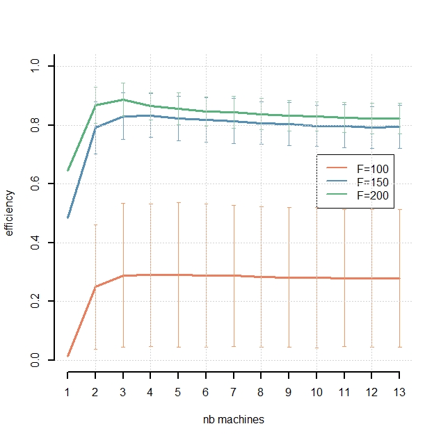
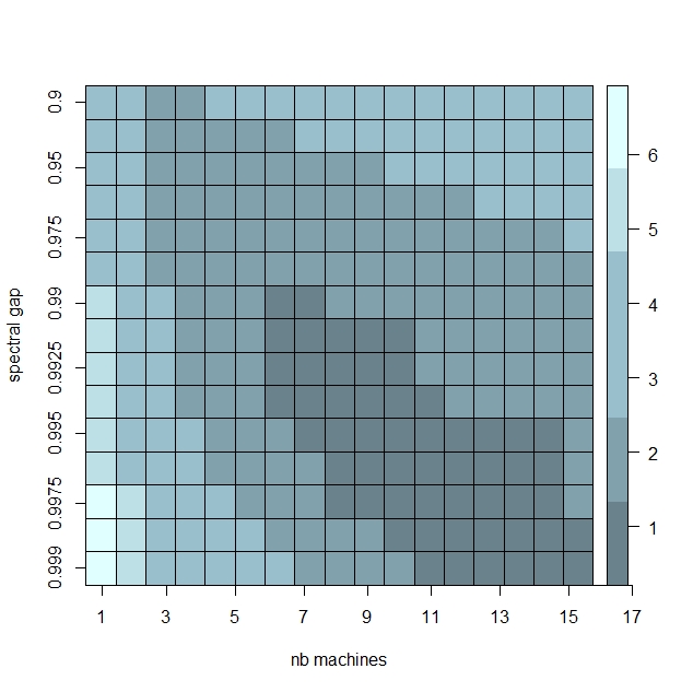
Figure 1: Left: Interplay between number of strong features and efficiency. Right: Interplay between spectral gap and optimal number of machines.

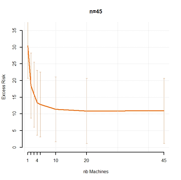
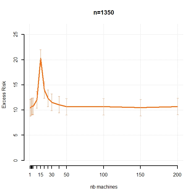
Figure 2: MSDYear dataset. Left: Data splitting reduces the test error in the presence of overparameterization. Right: The test error has a peak for $M=n/d$ and decreases as local overparameterization increases.

Appendix A Proofs of Section 3

In this section we provide all proofs of our results in Section 3.

A.1 Proofs of Section 3.1

Lemma A.1.

Let $n\in\mathbb{N}$, $\beta\in{\mathcal{H}}$. Define the empirical covariance operator by $\hat{\Sigma}=\frac{1}{n}{\mathbf{X}}^{T}{\mathbf{X}}$ and denote by

$$\tilde{\Pi}:=Id-{\mathbf{X}}^{T}({\mathbf{X}}{\mathbf{X}}^{T})^{\dagger}{\mathbf{X}}$$

the orthogonal projection onto the nullspace of ${\mathbf{X}}$. We have almost surely

$$||\Sigma^{1/2}\tilde{\Pi}\beta||^{2}\leq\mathopen{}\mathclose{{}\left|\IfEqCase{a}{{a}{\mathopen{}\mathclose{{}\left\langle\beta,(\Sigma-\hat{\Sigma})\beta}\right\rangle}{0}{\langle\beta,(\Sigma-\hat{\Sigma})\beta\rangle}{1}{\big{\langle}\beta,(\Sigma-\hat{\Sigma})\beta\big{\rangle}}{2}{\Big{\langle}\beta,(\Sigma-\hat{\Sigma})\beta\Big{\rangle}}{3}{\bigg{\langle}\beta,(\Sigma-\hat{\Sigma})\beta\bigg{\rangle}}{4}{\Bigg{\langle}\beta,(\Sigma-\hat{\Sigma})\beta\Bigg{\rangle}}}[]}\right|\;.$$

Proof of Lemma A.1.

For the proof we will use the following facts that can be found in e.g. [Ree12]:

• For all $\beta\in{\mathcal{H}}$ it holds: $||\beta||^{2}=\mathop{\rm Tr}\limits[\beta\otimes\beta]$.

• The trace is invariant under cyclic permutations: $\mathop{\rm Tr}\limits[ABC]=\mathop{\rm Tr}\limits[CAB]=\mathop{\rm Tr}\limits[BCA]$.

• If $A,B,C$ are self-adjoint, then the trace is invariant under any permutation:

  $$\mathop{\rm Tr}\limits[ABC]=\mathop{\rm Tr}\limits[(ABC)^{T}]=\mathop{\rm Tr}\limits[CBA]=\mathop{\rm Tr}\limits[ACB]\;.$$

• If $A$ has rank one, then $|\mathop{\rm Tr}\limits[A]|=||A||$. In particular, $\beta\otimes\beta$ has rank one and $|\mathop{\rm Tr}\limits[\beta\otimes\beta A]|=|\mathop{\rm Tr}\limits[A\beta\otimes\beta]|=||\beta\otimes\beta A||$.

First observe that

$$||\Sigma^{1/2}\tilde{\Pi}\beta^{*}||^{2} \stackrel{{\scriptstyle(a)}}{{=}}\mathopen{}\mathclose{{}\left|\mathop{\rm Tr}\limits\mathopen{}\mathclose{{}\left[\Sigma^{1/2}\tilde{\Pi}\beta\otimes\Sigma^{1/2}\tilde{\Pi}\beta}\right]}\right|$$

$$=\mathopen{}\mathclose{{}\left|\mathop{\rm Tr}\limits\mathopen{}\mathclose{{}\left[\Sigma^{1/2}\tilde{\Pi}(\beta\otimes\beta)\tilde{\Pi}\Sigma^{1/2}}\right]}\right|$$

$$\stackrel{{\scriptstyle(b)}}{{=}}\mathopen{}\mathclose{{}\left|\mathop{\rm Tr}\limits\mathopen{}\mathclose{{}\left[\tilde{\Pi}\Sigma\tilde{\Pi}(\beta\otimes\beta)}\right]}\right|$$

$$\stackrel{{\scriptstyle(d)}}{{=}}||\tilde{\Pi}\Sigma\tilde{\Pi}(\beta\otimes\beta)||=:\bullet\;.$$

Since $\tilde{\Pi}$ is an orthogonal projection onto the nullspace of ${\mathbf{X}}$ we have $||\tilde{\Pi}||\leq 1$ and

$$\tilde{\Pi}{\mathbf{X}}^{T}=0\;,\quad\tilde{\Pi}\hat{\Sigma}=0\;.$$

Hence, we find

$$\bullet =||\tilde{\Pi}(\Sigma-\hat{\Sigma})\tilde{\Pi}(\beta\otimes\beta)||$$

$$\leq||\tilde{\Pi}||\;||(\Sigma-\hat{\Sigma})\tilde{\Pi}(\beta\otimes\beta)||$$

$$\stackrel{{\scriptstyle(d)}}{{=}}|\mathop{\rm Tr}\limits[(\Sigma-\hat{\Sigma})\tilde{\Pi}(\beta\otimes\beta)]|$$

$$\stackrel{{\scriptstyle(c)}}{{=}}|\mathop{\rm Tr}\limits[\tilde{\Pi}(\Sigma-\hat{\Sigma})(\beta\otimes\beta)]|$$

$$\stackrel{{\scriptstyle(d)}}{{=}}||\tilde{\Pi}(\Sigma-\hat{\Sigma})(\beta\otimes\beta)||$$

$$\leq||(\Sigma-\hat{\Sigma})(\beta\otimes\beta)||$$

$$\stackrel{{\scriptstyle(d)}}{{=}}|\mathop{\rm Tr}\limits[(\Sigma-\hat{\Sigma})(\beta\otimes\beta)]|$$

$$=\mathopen{}\mathclose{{}\left|\IfEqCase{a}{{a}{\mathopen{}\mathclose{{}\left\langle\beta,(\Sigma-\hat{\Sigma})\beta}\right\rangle}{0}{\langle\beta,(\Sigma-\hat{\Sigma})\beta\rangle}{1}{\big{\langle}\beta,(\Sigma-\hat{\Sigma})\beta\big{\rangle}}{2}{\Big{\langle}\beta,(\Sigma-\hat{\Sigma})\beta\Big{\rangle}}{3}{\bigg{\langle}\beta,(\Sigma-\hat{\Sigma})\beta\bigg{\rangle}}{4}{\Bigg{\langle}\beta,(\Sigma-\hat{\Sigma})\beta\Bigg{\rangle}}}[]}\right|\;.$$

∎

The next Proposition is useful for bounding the bias in Lemma 3.1. We follow the lines of [NDR20], Lemma B.1, where a similar result is shown for gaussian variables. We extend this to the subgaussian setting.

Proposition A.2.

Suppose Assumption 2.2 is satisfied and let $\beta\in{\mathcal{H}}$. There exists a universal constant $c>0$ such that for any $\delta\geq 2e^{-c^{2}n}$, with probability at least $1-\delta$ we have

$$\mathopen{}\mathclose{{}\left|\IfEqCase{a}{{a}{\mathopen{}\mathclose{{}\left\langle\beta,(\Sigma-\hat{\Sigma})\beta}\right\rangle}{0}{\langle\beta,(\Sigma-\hat{\Sigma})\beta\rangle}{1}{\big{\langle}\beta,(\Sigma-\hat{\Sigma})\beta\big{\rangle}}{2}{\Big{\langle}\beta,(\Sigma-\hat{\Sigma})\beta\Big{\rangle}}{3}{\bigg{\langle}\beta,(\Sigma-\hat{\Sigma})\beta\bigg{\rangle}}{4}{\Bigg{\langle}\beta,(\Sigma-\hat{\Sigma})\beta\Bigg{\rangle}}}[]}\right|\leq\frac{4\sigma_{x}}{c}\;\log^{\frac{1}{2}}(2/\delta)\;\frac{||\Sigma^{\frac{1}{2}}\beta||^{2}}{\sqrt{n}}\;.$$

Proof of Proposition A.2.

Set $B^{2}:=\IfEqCase{a}{{a}{\mathopen{}\mathclose{{}\left\langle\Sigma\beta,\beta}\right\rangle}{0}{\langle\Sigma\beta,\beta\rangle}{1}{\big{\langle}\Sigma\beta,\beta\big{\rangle}}{2}{\Big{\langle}\Sigma\beta,\beta\Big{\rangle}}{3}{\bigg{\langle}\Sigma\beta,\beta\bigg{\rangle}}{4}{\Bigg{\langle}\Sigma\beta,\beta\Bigg{\rangle}}}[]$. We then write

$$\mathopen{}\mathclose{{}\left|\IfEqCase{a}{{a}{\mathopen{}\mathclose{{}\left\langle\beta,(\Sigma-\hat{\Sigma})\beta}\right\rangle}{0}{\langle\beta,(\Sigma-\hat{\Sigma})\beta\rangle}{1}{\big{\langle}\beta,(\Sigma-\hat{\Sigma})\beta\big{\rangle}}{2}{\Big{\langle}\beta,(\Sigma-\hat{\Sigma})\beta\Big{\rangle}}{3}{\bigg{\langle}\beta,(\Sigma-\hat{\Sigma})\beta\bigg{\rangle}}{4}{\Bigg{\langle}\beta,(\Sigma-\hat{\Sigma})\beta\Bigg{\rangle}}}[]}\right| =\mathopen{}\mathclose{{}\left|\IfEqCase{a}{{a}{\mathopen{}\mathclose{{}\left\langle\beta,\hat{\Sigma}\beta}\right\rangle}{0}{\langle\beta,\hat{\Sigma}\beta\rangle}{1}{\big{\langle}\beta,\hat{\Sigma}\beta\big{\rangle}}{2}{\Big{\langle}\beta,\hat{\Sigma}\beta\Big{\rangle}}{3}{\bigg{\langle}\beta,\hat{\Sigma}\beta\bigg{\rangle}}{4}{\Bigg{\langle}\beta,\hat{\Sigma}\beta\Bigg{\rangle}}}[]-\IfEqCase{a}{{a}{\mathopen{}\mathclose{{}\left\langle\beta,\Sigma\beta}\right\rangle}{0}{\langle\beta,\Sigma\beta\rangle}{1}{\big{\langle}\beta,\Sigma\beta\big{\rangle}}{2}{\Big{\langle}\beta,\Sigma\beta\Big{\rangle}}{3}{\bigg{\langle}\beta,\Sigma\beta\bigg{\rangle}}{4}{\Bigg{\langle}\beta,\Sigma\beta\Bigg{\rangle}}}[]}\right|$$

$$=\mathopen{}\mathclose{{}\left|\frac{1}{n}\sum_{j=1}^{n}\IfEqCase{a}{{a}{\mathopen{}\mathclose{{}\left\langle\beta,(x_{j}\otimes x_{j})\beta}\right\rangle}{0}{\langle\beta,(x_{j}\otimes x_{j})\beta\rangle}{1}{\big{\langle}\beta,(x_{j}\otimes x_{j})\beta\big{\rangle}}{2}{\Big{\langle}\beta,(x_{j}\otimes x_{j})\beta\Big{\rangle}}{3}{\bigg{\langle}\beta,(x_{j}\otimes x_{j})\beta\bigg{\rangle}}{4}{\Bigg{\langle}\beta,(x_{j}\otimes x_{j})\beta\Bigg{\rangle}}}[]-B^{2}}\right|$$

$$=\mathopen{}\mathclose{{}\left|\frac{B^{2}}{n}\mathopen{}\mathclose{{}\left(\sum_{j=1}^{n}\frac{\IfEqCase{a}{{a}{\mathopen{}\mathclose{{}\left\langle\beta,x_{j}}\right\rangle}{0}{\langle\beta,x_{j}\rangle}{1}{\big{\langle}\beta,x_{j}\big{\rangle}}{2}{\Big{\langle}\beta,x_{j}\Big{\rangle}}{3}{\bigg{\langle}\beta,x_{j}\bigg{\rangle}}{4}{\Bigg{\langle}\beta,x_{j}\Bigg{\rangle}}}[]^{2}}{B^{2}}-1}\right)}\right|\;.$$ (A.1)

We next show that for any $j=1,...,n$, the real valued variables $z_{j}:=\frac{\IfEqCase{a}{{a}{\mathopen{}\mathclose{{}\left\langle\beta,x_{j}}\right\rangle}{0}{\langle\beta,x_{j}\rangle}{1}{\big{\langle}\beta,x_{j}\big{\rangle}}{2}{\Big{\langle}\beta,x_{j}\Big{\rangle}}{3}{\bigg{\langle}\beta,x_{j}\bigg{\rangle}}{4}{\Bigg{\langle}\beta,x_{j}\Bigg{\rangle}}}[]}{B}$ are $(\sigma_{x}^{2},id)$-subgaussian. Indeed, by Assumption 2.2 and Definition 2.1 we find for all $\alpha\in\mathbb{R}$

$$\mathbb{E}\mathopen{}\mathclose{{}\left[e^{\alpha z_{j}}}\right] =\mathbb{E}\mathopen{}\mathclose{{}\left[e^{\IfEqCase{a}{{a}{\mathopen{}\mathclose{{}\left\langle\frac{\alpha}{B}\beta,x_{j}}\right\rangle}{0}{\langle\frac{\alpha}{B}\beta,x_{j}\rangle}{1}{\big{\langle}\frac{\alpha}{B}\beta,x_{j}\big{\rangle}}{2}{\Big{\langle}\frac{\alpha}{B}\beta,x_{j}\Big{\rangle}}{3}{\bigg{\langle}\frac{\alpha}{B}\beta,x_{j}\bigg{\rangle}}{4}{\Bigg{\langle}\frac{\alpha}{B}\beta,x_{j}\Bigg{\rangle}}}[]}}\right]$$

$$\leq e^{\frac{\sigma_{x}^{2}}{2}\IfEqCase{a}{{a}{\mathopen{}\mathclose{{}\left\langle\Sigma\frac{\alpha}{B}\beta,\frac{\alpha}{B}\beta}\right\rangle}{0}{\langle\Sigma\frac{\alpha}{B}\beta,\frac{\alpha}{B}\beta\rangle}{1}{\big{\langle}\Sigma\frac{\alpha}{B}\beta,\frac{\alpha}{B}\beta\big{\rangle}}{2}{\Big{\langle}\Sigma\frac{\alpha}{B}\beta,\frac{\alpha}{B}\beta\Big{\rangle}}{3}{\bigg{\langle}\Sigma\frac{\alpha}{B}\beta,\frac{\alpha}{B}\beta\bigg{\rangle}}{4}{\Bigg{\langle}\Sigma\frac{\alpha}{B}\beta,\frac{\alpha}{B}\beta\Bigg{\rangle}}}[]}$$

$$=e^{\frac{\sigma_{x}^{2}}{2}\alpha^{2}}\;.$$ (A.2)

For bounding (A.1) with high probability we use the fact that for any $j=1,...,n$ the random variable $z_{j}^{2}-1$ is $16\sigma_{x}^{2}$-subexponential. Indeed, this follows from (A.1) and results in [Ver18, Section 2] that are condensed in [BLLT20, Lemma S.4]. Next, Bernstein’s inequality for the independent and mean zero subexponential variables $z_{1},...,z_{n}$ in [Ver18, Theorem 2.8.2] shows that there exists a universal constant $c>0$ such that for all $t\geq 0$, with probability at least

$$1-2\exp\mathopen{}\mathclose{{}\left(-c^{2}\min\mathopen{}\mathclose{{}\left\{\frac{t^{2}}{16\sigma_{x}^{2}n},\frac{t}{4\sigma_{x}}}\right\}}\right)$$

we have

$$\mathopen{}\mathclose{{}\left|\frac{B^{2}}{n}\mathopen{}\mathclose{{}\left(\sum_{j=1}^{n}\frac{\IfEqCase{a}{{a}{\mathopen{}\mathclose{{}\left\langle\beta,x_{j}}\right\rangle}{0}{\langle\beta,x_{j}\rangle}{1}{\big{\langle}\beta,x_{j}\big{\rangle}}{2}{\Big{\langle}\beta,x_{j}\Big{\rangle}}{3}{\bigg{\langle}\beta,x_{j}\bigg{\rangle}}{4}{\Bigg{\langle}\beta,x_{j}\Bigg{\rangle}}}[]^{2}}{B^{2}}-1}\right)}\right|\leq\frac{B^{2}}{n}\;t\;.$$

Assuming that $t\leq 4\sigma_{x}n$ we find that

$$\min\mathopen{}\mathclose{{}\left\{\frac{t^{2}}{16\sigma_{x}^{2}n},\frac{t}{4\sigma_{x}}}\right\}=\frac{t^{2}}{16\sigma_{x}^{2}n}\;.$$

Setting now $\delta=2e^{-\frac{c^{2}}{16\sigma_{x}^{2}}\frac{t^{2}}{n}}$ we finally get

$$\mathopen{}\mathclose{{}\left|\IfEqCase{a}{{a}{\mathopen{}\mathclose{{}\left\langle\beta,(\Sigma-\hat{\Sigma})\beta}\right\rangle}{0}{\langle\beta,(\Sigma-\hat{\Sigma})\beta\rangle}{1}{\big{\langle}\beta,(\Sigma-\hat{\Sigma})\beta\big{\rangle}}{2}{\Big{\langle}\beta,(\Sigma-\hat{\Sigma})\beta\Big{\rangle}}{3}{\bigg{\langle}\beta,(\Sigma-\hat{\Sigma})\beta\bigg{\rangle}}{4}{\Bigg{\langle}\beta,(\Sigma-\hat{\Sigma})\beta\Bigg{\rangle}}}[]}\right|\leq\frac{4\sigma_{x}}{c}\frac{||\Sigma^{\frac{1}{2}}\beta||^{2}}{\sqrt{n}}\log^{\frac{1}{2}}(2/\delta)\;.$$

with probability at least $1-\delta$, for all $\delta\geq 2e^{-c^{2}n}$. ∎

The next result establishes a bound for the single machine variance. This is a first step for bounding the variance from Lemma 3.1 in the distributed setting.

Proposition A.3.

Let $n\in\mathbb{N}$ and suppose Assumption 2.2 is satisfied. Define

$$\widehat{C}:=({\mathbf{X}}{\mathbf{X}}^{T})^{-1}{\mathbf{X}}\Sigma{\mathbf{X}}^{T}({\mathbf{X}}{\mathbf{X}}^{T})^{-1}\;.$$

There exists a universal constant $c>1$ and a $0\leq k_{n}^{*}\leq\frac{n}{c}$ such that with probability at least $1-7e^{-\frac{n}{c}}$ it holds

$$\mathop{\rm Tr}\limits[\widehat{C}]\leq c\mathopen{}\mathclose{{}\left(\frac{k_{n}^{*}}{n}+n\;\frac{\sum_{j>k_{n}^{*}}\lambda_{j}^{2}}{\mathopen{}\mathclose{{}\left(\sum_{j>k_{n}^{*}}\lambda_{j}}\right)^{2}}}\right)\;,$$

where $(\lambda_{j})_{j\in\mathbb{N}}$ are the eigenvalues of $\Sigma$, arranged in decreasing order.

Proof of Proposition A.3.

The proof follows from [BLLT20, Lemma 6] and [BLLT20, Lemma 11]. ∎

Combining now the above results allows to prove Lemma 3.1.

Proof of Lemma 3.1.

We first derive a bound for the bias. Linearity of the expectation and (2.1) yields

$$\mathbb{E}_{\varepsilon}[\bar{\beta}_{M}]=\frac{1}{M}\sum_{m=1}^{M}X_{m}^{T}(X_{m}X_{m}^{T})^{\dagger}\mathbb{E}_{\varepsilon}[Y_{m}]=\frac{1}{M}\sum_{m=1}^{M}X_{m}^{T}(X_{m}X_{m}^{T})^{\dagger}X_{m}\beta^{*}\;,$$ (A.3)

since, conditionally on the inputs ${\mathbf{X}}$, the noise is centered. Hence

$$\beta^{*}-\mathbb{E}_{\epsilon}[\bar{\beta}_{M}] =\frac{1}{M}\sum_{m=1}^{M}\tilde{\Pi}_{m}\beta^{*}\;,$$

where we denote by

$$\tilde{\Pi}_{m}:=Id-{\mathbf{X}}_{m}^{T}({\mathbf{X}}_{m}{\mathbf{X}}_{m}^{T})^{\dagger}{\mathbf{X}}_{m}$$

the orthogonal projection onto the nullspace of ${\mathbf{X}}_{m}$. Convexity and Lemma A.1 allow to deduce

$$\widehat{{\rm Bias}}(\bar{\beta}_{M}) =||\Sigma^{1/2}(\mathbb{E}_{\epsilon}[\bar{\beta}_{M}]-\beta^{*})||^{2}$$

$$\leq\frac{1}{M}\sum_{m=1}^{M}||\Sigma^{1/2}\tilde{\Pi}_{m}\beta^{*}||^{2}$$

$$\leq\frac{1}{M}\sum_{m=1}^{M}\mathopen{}\mathclose{{}\left|\IfEqCase{a}{{a}{\mathopen{}\mathclose{{}\left\langle\beta^{*},(\Sigma-\hat{\Sigma}_{m})\beta^{*}}\right\rangle}{0}{\langle\beta^{*},(\Sigma-\hat{\Sigma}_{m})\beta^{*}\rangle}{1}{\big{\langle}\beta^{*},(\Sigma-\hat{\Sigma}_{m})\beta^{*}\big{\rangle}}{2}{\Big{\langle}\beta^{*},(\Sigma-\hat{\Sigma}_{m})\beta^{*}\Big{\rangle}}{3}{\bigg{\langle}\beta^{*},(\Sigma-\hat{\Sigma}_{m})\beta^{*}\bigg{\rangle}}{4}{\Bigg{\langle}\beta^{*},(\Sigma-\hat{\Sigma}_{m})\beta^{*}\Bigg{\rangle}}}[]}\right|\;.$$

Next, we derive a bound for the variance. By definition of the variance, (2.2) and (A.3) we find

$$\widehat{{\rm Var}}(\bar{\beta}_{M}) =\mathbb{E}_{\epsilon}\mathopen{}\mathclose{{}\left[||\Sigma^{1/2}(\bar{\beta}_{M}-\mathbb{E}_{\epsilon}[\bar{\beta}_{M}])||_{2}^{2}}\right]$$

$$=\mathbb{E}_{\varepsilon}\Big{[}||\Sigma^{1/2}\Big{(}\frac{1}{M}\sum_{m=1}^{M}\hat{\beta}^{(m)}-X_{m}^{T}(X_{m}X_{m}^{T})^{\dagger}X_{m}\beta^{*}\Big{)}||^{2}\Big{]}$$

$$=\mathbb{E}_{\varepsilon}\Big{[}||\Sigma^{1/2}\Big{(}\frac{1}{M}\sum_{m=1}^{M}X_{m}^{T}(X_{m}X_{m}^{T})^{\dagger}(Y_{m}-X_{m}\beta^{*})\Big{)}||^{2}\Big{]}$$

$$=\mathbb{E}_{\varepsilon}\Big{[}||\Sigma^{1/2}\Big{(}\frac{1}{M}\sum_{m=1}^{M}X_{m}^{T}(X_{m}X_{m}^{T})^{\dagger}\varepsilon_{m}\Big{)}||^{2}\Big{]}$$

$$=\mathbb{E}_{\varepsilon}\Big{[}||\Sigma^{1/2}\Big{(}\frac{1}{M}\sum_{m=1}^{M}X_{m}^{\dagger}\varepsilon_{m}\Big{)}||^{2}\Big{]}\;.$$

In the last step we use $X_{m}^{T}(X_{m}X_{m}^{T})^{\dagger}=X_{m}^{\dagger}$. Recall that for any $\beta\in{\mathcal{H}}$ we may write $||\beta||^{2}=\mathop{\rm Tr}\limits[\beta\otimes\beta]$. Hence,

$$||\Sigma^{1/2}\Big{(}\frac{1}{M}\sum_{m=1}^{M}X_{m}^{\dagger}\varepsilon_{m}\Big{)}||^{2}$$

$$\mathop{\rm Tr}\limits\mathopen{}\mathclose{{}\left[\mathopen{}\mathclose{{}\left(\frac{1}{M}\sum_{m=1}^{M}\Sigma^{1/2}X_{m}^{\dagger}\varepsilon_{m}}\right)\otimes\mathopen{}\mathclose{{}\left(\frac{1}{M}\sum_{m^{\prime}=1}^{M}\Sigma^{1/2}X_{m^{\prime}}^{\dagger}\varepsilon_{m^{\prime}}}\right)}\right]$$

$$=\frac{1}{M^{2}}\sum_{m,m^{\prime}=1}^{M}\mathop{\rm Tr}\limits\mathopen{}\mathclose{{}\left[\Sigma^{1/2}X_{m}^{\dagger}\varepsilon_{m}\otimes\varepsilon_{m^{\prime}}(X_{m^{\prime}}^{\dagger})^{T}\Sigma^{1/2}}\right]\;.$$

By linearity of the trace and independence, taking the expectation gives $\mathbb{E}_{\varepsilon}[\varepsilon_{m}\otimes\varepsilon_{m^{\prime}}]=0$ for any $m\not=m^{\prime}$ and the sum reduces to

$$\mathbb{E}_{\varepsilon}\Big{[}||\Sigma^{1/2}\Big{(}\frac{1}{M}\sum_{m=1}^{M}X_{m}^{\dagger}\varepsilon_{m}\Big{)}||^{2}\Big{]} =\frac{1}{M^{2}}\sum_{m=1}^{M}\mathbb{E}_{\varepsilon}\Big{[}\mathop{\rm Tr}\limits\Big{[}\Sigma^{1/2}X_{m}^{\dagger}\varepsilon_{m}\otimes\varepsilon_{m}(X_{m}^{\dagger})^{T}\Sigma^{1/2}\Big{]}\Big{]}$$

$$=\frac{1}{M^{2}}\sum_{m=1}^{M}\mathbb{E}_{\varepsilon}\Big{[}||\Sigma^{1/2}X_{m}^{\dagger}\varepsilon_{m}||^{2}\Big{]}$$

$$=\frac{1}{M^{2}}\sum_{m=1}^{M}\mathbb{E}_{\varepsilon}\Big{[}\IfEqCase{a}{{a}{\mathopen{}\mathclose{{}\left\langle\varepsilon_{m},C_{m}\varepsilon_{m}}\right\rangle}{0}{\langle\varepsilon_{m},C_{m}\varepsilon_{m}\rangle}{1}{\big{\langle}\varepsilon_{m},C_{m}\varepsilon_{m}\big{\rangle}}{2}{\Big{\langle}\varepsilon_{m},C_{m}\varepsilon_{m}\Big{\rangle}}{3}{\bigg{\langle}\varepsilon_{m},C_{m}\varepsilon_{m}\bigg{\rangle}}{4}{\Bigg{\langle}\varepsilon_{m},C_{m}\varepsilon_{m}\Bigg{\rangle}}}[]\Big{]}\;,$$ (A.4)

where we set

$$C_{m}:=\mathopen{}\mathclose{{}\left(X_{m}^{\dagger}}\right)^{T}\Sigma X_{m}^{\dagger}\;.$$

To proceed, we apply a conditional subgaussian version of the Hanson-Wright inequality taken from [PG19, Lemma 35]. This gives almost surely conditional on the data $X_{m}$, for all $t\geq 0$, with probability at least $1-e^{-t}$ (w.r.t. the noise)

$$\IfEqCase{a}{{a}{\mathopen{}\mathclose{{}\left\langle\varepsilon_{m},C_{m}\varepsilon_{m}}\right\rangle}{0}{\langle\varepsilon_{m},C_{m}\varepsilon_{m}\rangle}{1}{\big{\langle}\varepsilon_{m},C_{m}\varepsilon_{m}\big{\rangle}}{2}{\Big{\langle}\varepsilon_{m},C_{m}\varepsilon_{m}\Big{\rangle}}{3}{\bigg{\langle}\varepsilon_{m},C_{m}\varepsilon_{m}\bigg{\rangle}}{4}{\Bigg{\langle}\varepsilon_{m},C_{m}\varepsilon_{m}\Bigg{\rangle}}}[] \leq\tau^{2}\mathop{\rm Tr}\limits[C_{m}]+2\tau^{2}t||C_{m}||+2\tau^{2}\sqrt{t^{2}||C_{m}||^{2}+t\mathop{\rm Tr}\limits[C_{m}^{2}]}$$

$$\leq 4\tau^{2}\mathop{\rm Tr}\limits[C_{m}]\;(t+1)\;,$$

where we use that $||C_{m}||\leq\mathop{\rm Tr}\limits[C_{m}]$ and $\mathop{\rm Tr}\limits[C_{m}^{2}]\leq||C_{m}||\mathop{\rm Tr}\limits[C_{m}]\leq\mathop{\rm Tr}\limits[C_{m}]^{2}$. From [BM18, Lemma C.1] we obtain after integration for the conditional expectation

$$\mathbb{E}_{\varepsilon}\mathopen{}\mathclose{{}\left[\IfEqCase{a}{{a}{\mathopen{}\mathclose{{}\left\langle\varepsilon_{m},C_{m}\varepsilon_{m}}\right\rangle}{0}{\langle\varepsilon_{m},C_{m}\varepsilon_{m}\rangle}{1}{\big{\langle}\varepsilon_{m},C_{m}\varepsilon_{m}\big{\rangle}}{2}{\Big{\langle}\varepsilon_{m},C_{m}\varepsilon_{m}\Big{\rangle}}{3}{\bigg{\langle}\varepsilon_{m},C_{m}\varepsilon_{m}\bigg{\rangle}}{4}{\Bigg{\langle}\varepsilon_{m},C_{m}\varepsilon_{m}\Bigg{\rangle}}}[]}\right]\leq 8\tau^{2}\mathop{\rm Tr}\limits[C_{m}]\;.$$

Inserting the last bound into (A.1) finally gives almost surely

$$\widehat{{\rm Var}}(\bar{\beta}_{M})\leq\frac{8\tau^{2}}{M^{2}}\sum_{m=1}^{M}\mathop{\rm Tr}\limits[C_{m}]\;.$$

∎

Finally, we give the proof of our main result, a general upper bound for distributed ridgeless regression.

Proof of Theorem 3.5.

We start with bounding the bias term.
Bounding the Bias. Recall that by Lemma 3.1 we have almost surely

$$\widehat{{\rm Bias}}(\bar{\beta}_{M})\leq\frac{1}{M}\sum_{m=1}^{M}\mathopen{}\mathclose{{}\left|\IfEqCase{a}{{a}{\mathopen{}\mathclose{{}\left\langle\beta^{*},(\Sigma-\hat{\Sigma}_{m})\beta^{*}}\right\rangle}{0}{\langle\beta^{*},(\Sigma-\hat{\Sigma}_{m})\beta^{*}\rangle}{1}{\big{\langle}\beta^{*},(\Sigma-\hat{\Sigma}_{m})\beta^{*}\big{\rangle}}{2}{\Big{\langle}\beta^{*},(\Sigma-\hat{\Sigma}_{m})\beta^{*}\Big{\rangle}}{3}{\bigg{\langle}\beta^{*},(\Sigma-\hat{\Sigma}_{m})\beta^{*}\bigg{\rangle}}{4}{\Bigg{\langle}\beta^{*},(\Sigma-\hat{\Sigma}_{m})\beta^{*}\Bigg{\rangle}}}[]}\right|\;.$$

Proposition A.2 gives for all $\delta\geq 2e^{-c^{2}\frac{n}{M}}$, with probability at least $1-\delta$

$$\mathopen{}\mathclose{{}\left|\IfEqCase{a}{{a}{\mathopen{}\mathclose{{}\left\langle\beta^{*},(\Sigma-\hat{\Sigma}_{m})\beta^{*}}\right\rangle}{0}{\langle\beta^{*},(\Sigma-\hat{\Sigma}_{m})\beta^{*}\rangle}{1}{\big{\langle}\beta^{*},(\Sigma-\hat{\Sigma}_{m})\beta^{*}\big{\rangle}}{2}{\Big{\langle}\beta^{*},(\Sigma-\hat{\Sigma}_{m})\beta^{*}\Big{\rangle}}{3}{\bigg{\langle}\beta^{*},(\Sigma-\hat{\Sigma}_{m})\beta^{*}\bigg{\rangle}}{4}{\Bigg{\langle}\beta^{*},(\Sigma-\hat{\Sigma}_{m})\beta^{*}\Bigg{\rangle}}}[]}\right|\leq\frac{4\sigma_{x}}{c}\;\log^{\frac{1}{2}}(2/\delta)\;||\Sigma^{\frac{1}{2}}\beta^{*}||^{2}\sqrt{\frac{M}{n}}\;,$$

for some universal constant $c>0$. Performing now a union bound and invoking Assumption 3.2 finally gives with probability at least $1-\delta$

$$\mathbb{E}_{\beta^{*}}[\widehat{{\rm Bias}}(\bar{\beta}_{M})]\leq\frac{4\sigma_{x}}{c}\;\log^{\frac{1}{2}}(2M/\delta)\;\mathop{\rm Tr}\limits[\Sigma\Theta]\sqrt{\frac{M}{n}}\;,$$

where we use that

$$\mathbb{E}_{\beta^{*}}[||\Sigma^{\frac{1}{2}}\beta^{*}||^{2}]=\mathop{\rm Tr}\limits\mathopen{}\mathclose{{}\left[\mathbb{E}_{\beta^{*}}[\Sigma\beta^{*}\otimes\beta^{*}]}\right]=\mathop{\rm Tr}\limits[\Sigma\Theta]\;.$$

Bounding the Variance. Applying Lemma 3.1 once more we have almost surely

$$\widehat{{\rm Var}}(\bar{\beta}_{M})\leq\frac{8\tau^{2}}{M^{2}}\sum_{m=1}^{M}\mathop{\rm Tr}\limits[C_{m}]\;.$$

With Lemma A.3 together with a union bound we get with probability at least $1-7Me^{-\frac{n}{c_{2}M}}$

$$\widehat{{\rm Var}}(\bar{\beta}_{M}) \leq\frac{8c_{2}\tau^{2}}{M^{2}}\sum_{m=1}^{M}\mathopen{}\mathclose{{}\left(\frac{M}{n}k_{n/M}^{*}+\frac{n}{M}\;\frac{\sum_{j>k_{n/M}^{*}}\lambda_{j}^{2}}{\mathopen{}\mathclose{{}\left(\sum_{j>k_{n/M}^{*}}\lambda_{j}}\right)^{2}}}\right)$$

$$=8c_{2}\tau^{2}\mathopen{}\mathclose{{}\left(\frac{k_{n/M}^{*}}{n}+\frac{n}{M^{2}}\;\frac{\sum_{j>k_{n/M}^{*}}\lambda_{j}^{2}}{\mathopen{}\mathclose{{}\left(\sum_{j>k_{n/M}^{*}}\lambda_{j}}\right)^{2}}}\right)\;,$$

for some constant $c_{2}>1$ and $0\leq k_{n/M}^{*}\leq\frac{n}{c_{2}M}$. ∎

A.2 Proofs of Section 3.2

This section establishes a refined upper bound for the excess risk in the infinite dimensional setting under the specific Assumptions 3.6, 3.7. We start with a preliminary Lemma that is needed to estimate the variance.

Lemma A.4.

Suppose all assumptions of Theorem 3.5 are satisfied. Assume that $\lambda_{j}(\Sigma)=j^{-(1+\varepsilon_{n})}$ for a positive sequence $(\varepsilon_{n})_{n\in\mathbb{N}}$. We have

1. $\frac{k_{\frac{n}{M}}^{*}}{n}\leq a\;\frac{\varepsilon_{n}}{M}$.

2. For any $n$ sufficiently large, $\frac{n}{M^{2}}\;\frac{1}{R_{k_{\frac{n}{M}}^{*}}(\Sigma)}\leq\frac{6}{a}\;\frac{\varepsilon_{n}}{M}$. If $M\lesssim n\varepsilon_{n}$, then $k^{*}_{\frac{n}{M}}\gtrsim 1$.

Proof of Lemma A.4.

1. We follow the lines of [BLLT20], Proof of Theorem 31, by lower bounding the effective rank $r_{k}(\Sigma)$. With Lemma 14 in [MNR19] we may write

   $$r_{k}(\Sigma) =(k+1)^{1+\varepsilon_{n}}\sum_{j>k}j^{-(1+\varepsilon_{n})}$$

   $$\geq(k+1)^{1+\varepsilon_{n}}\int_{k+1}^{\infty}t^{-(1+\varepsilon_{n})}$$

   $$=\frac{k+1}{\varepsilon_{n}}\;.$$

   By Definition 3.4, the effective dimension $k^{*}_{\frac{n}{M}}$ is the smallest number satisfying $r_{k^{*}_{\frac{n}{M}}}(\Sigma)\geq a\frac{n}{M}$. Hence, $k^{*}_{\frac{n}{M}}\leq a\varepsilon_{n}\frac{n}{M}$.

2. A short calculation shows that

   $$R_{k}(\Sigma)\geq\frac{k}{\varepsilon_{n}^{2}}\mathopen{}\mathclose{{}\left(1-\frac{1}{k+1}}\right)^{2\varepsilon_{n}}\;,\quad r_{k}(\Sigma)\leq\frac{2k}{\varepsilon_{n}}e^{\varepsilon_{n}}\;.$$

   Following the arguments in the proof of Theorem 31 in [BLLT20] we find also in the distributed setting that $k^{*}_{\frac{n}{M}}\geq\frac{a\varepsilon}{3}\frac{n}{M}$ for sufficiently large $n$. Hence,

   $$R_{k^{*}_{\frac{n}{M}}}(\Sigma)\geq\frac{a\varepsilon_{n}}{6}\frac{n}{M}\;.$$

∎

The second preliminary Lemma will help to bound the bias.

Lemma A.5.

Suppose Assumption 3.7 is satisfied. Let $\alpha\geq 0$. Then

$$\mathop{\rm Tr}\limits[\Sigma^{1+\alpha}]\;=\;\sum_{j=1}^{\infty}\mathopen{}\mathclose{{}\left(\frac{1}{j}}\right)^{(1+\alpha)(1+\varepsilon_{n})}\;\leq\;\frac{1}{\alpha+\varepsilon_{n}(1+\alpha)}\;\leq\;\mathopen{}\mathclose{{}\left\{{\begin{array}[]{cc}\alpha=0&:\;\frac{1}{\varepsilon_{n}}\\ \alpha>0&:\;\frac{1}{\alpha}\\ \end{array}}}\right.\;.$$

Proof of Lemma A.5.

Let $\beta=(1+\alpha)(1+\varepsilon_{n})$. The infinite sum can easily be bounded by an integral

$$\sum_{j=1}^{\infty}\mathopen{}\mathclose{{}\left(\frac{1}{j}}\right)^{\beta} \leq\int_{1}^{\infty}t^{-\beta}dt=\frac{1}{\beta-1}\;,$$

see e.g. Lemma 14 in [MNR19]. ∎

Combining now Lemma A.4 and Lemma A.5 with Theorem 3.5 gives the main result in this section.

Proof of Proposition 3.8.

For bounding the bias we apply Lemma A.5

$$\mathop{\rm Tr}\limits[\Sigma\Theta]=\mathop{\rm Tr}\limits[\Sigma^{1+\alpha}]=\sum_{j\in\mathbb{N}}\lambda^{1+\alpha}_{j}(\Sigma)\leq\frac{1}{\alpha}\mathbb{1}\{\alpha>0\}+\frac{1}{\varepsilon_{n}}\mathbb{1}\{\alpha=0\}=:C_{\alpha,n}\;.$$

Combining this with Lemma A.4, Lemma 3.1 and Theorem 3.5 leads to

$$\mathbb{E}_{\beta^{*},\epsilon}\mathopen{}\mathclose{{}\left[||\Sigma^{\frac{1}{2}}(\bar{\beta}_{M}-\beta^{*})||^{2}}\right]$$

$$\leq\frac{4\sigma_{x}}{c_{1}}\log^{\frac{1}{2}}\mathopen{}\mathclose{{}\left(\frac{2M}{\delta}}\right)\mathop{\rm Tr}\limits[\Sigma^{1+\alpha}]\sqrt{\frac{M}{n}}+8c_{2}\tau^{2}\mathopen{}\mathclose{{}\left(a\;\frac{\varepsilon_{n}}{M}+\frac{6}{a}\;\frac{\varepsilon_{n}}{M}}\right)$$

$$\leq\frac{4\sigma_{x}}{c_{1}}C_{\alpha,n}\log^{\frac{1}{2}}\mathopen{}\mathclose{{}\left(\frac{2M}{\delta}}\right)\sqrt{\frac{M}{n}}+8c_{2}c_{a}\tau^{2}\frac{\varepsilon_{n}}{M}\;,$$

holding with probability at least $1-\delta-7Me^{-\frac{n}{c_{2}M}}$, for any $\delta\geq 2e^{-c_{1}^{2}\frac{n}{M}}$. Here, we set $c_{a}=\max\{a,6/a\}$. The result follows with $c_{3}=4/c_{1}$ and $c_{4}=8c_{2}c_{a}$. ∎

Proof of Corollary 3.9 and Corollary 3.10.

We determine the maximum number of local nodes by balancing bias and variance. To this end, firstly note that $1\leq\log^{\frac{1}{2}}\mathopen{}\mathclose{{}\left(\frac{4M_{n}}{\delta}}\right)$. Setting now

$$A:=c_{3}\sigma_{x}\frac{C_{\alpha,n}}{\sqrt{n}}\;,\quad B:=c_{4}\tau^{2}\varepsilon_{n}\;,$$

we find that

$$A\sqrt{M}=\frac{B}{M}\quad\Longleftrightarrow\quad M=\mathopen{}\mathclose{{}\left(\frac{B}{A}}\right)^{2/3}\;.$$

Hence, the value

$$M_{n}:=C_{\tau,\sigma_{x}}\mathopen{}\mathclose{{}\left(\frac{\varepsilon_{n}\sqrt{n}}{C_{\alpha,n}}}\right)^{2/3}\;,\quad C_{\tau,\sigma_{x}}=\mathopen{}\mathclose{{}\left(\frac{c_{4}\tau^{2}}{c_{3}\sigma_{x}}}\right)^{2/3}$$

trades off bias and variance and the excess risk is bounded as

$$\mathbb{E}_{\beta^{*},\epsilon}\mathopen{}\mathclose{{}\left[||\Sigma^{\frac{1}{2}}(\bar{\beta}_{M_{n}}-\beta^{*})||^{2}}\right] \leq 2c_{4}\tau^{2}\log^{\frac{1}{2}}\mathopen{}\mathclose{{}\left(\frac{4M_{n}}{\delta}}\right)\frac{\varepsilon_{n}}{M_{n}}$$

$$=C^{\prime}_{\tau,\sigma_{x}}\log^{\frac{1}{2}}\mathopen{}\mathclose{{}\left(\frac{4M_{n}}{\delta}}\right)\mathopen{}\mathclose{{}\left(\frac{C^{2}_{\alpha,n}\varepsilon_{n}}{n}}\right)^{1/3}\;,$$

where $C^{\prime}_{\tau,\sigma_{x}}=\frac{2c_{4}\tau^{2}}{C_{\tau,\sigma_{x}}}$. ∎

A.3 Proofs of Section 3.3

In this section we provide the proofs for our results in finite dimension with $dim({\mathcal{H}})=d<\infty$ from Section 3.3. We start with two preliminary Lemmata.

Lemma A.6.

Suppose Assumption 3.12 holds. Then

$$\mathop{\rm Tr}\limits[\Sigma\Theta]\leq\frac{2\cdot{\rm SNR}}{d}\;F\;.$$

Proof of Lemma A.6.

By Assumption 3.12 with $\Theta=\frac{{\rm SNR}}{d}\;Id_{d}$ and since $d\rho_{2}\leq F$ we easily obtain

$$\mathop{\rm Tr}\limits[\Sigma\Theta] =\frac{{\rm SNR}}{d}\;\mathop{\rm Tr}\limits[\Sigma]$$

$$=\frac{{\rm SNR}}{d}\;\mathopen{}\mathclose{{}\left(\sum_{j=1}^{F}\rho_{1}+\sum_{j=F+1}^{d}\rho_{2}}\right)$$

$$=\frac{{\rm SNR}}{d}\;\mathopen{}\mathclose{{}\left(F\rho_{1}+(d-F)\rho_{2}}\right)$$

$$=\frac{{\rm SNR}}{d}\;\mathopen{}\mathclose{{}\left((\rho_{1}-\rho_{2})F+d\rho_{2}}\right)$$

$$\leq\frac{{\rm SNR}}{d}\;(\rho_{1}-\rho_{2}+1)F$$

$$\leq\frac{2{\rm SNR}}{d}\;F\;.$$

In the last step we use that $\rho_{1}=1$ and $-\rho_{2}\leq 0$. ∎

Lemma A.7.

Suppose Assumptions of Theorem 3.5 are satisfied. If additionally Assumption 3.11 holds, then with probability at least $1-7Me^{-\frac{n}{c_{2}M}}$

$$\widehat{{\rm Var}}(\bar{\beta}_{M}) \leq 16c_{2}\tau^{2}\;\frac{1}{(\rho_{1}-\rho_{2})^{2}}\;\frac{n}{M^{2}}\;\frac{1}{F}\;.$$

Proof of Lemma A.7.

We bound the first term $\frac{k_{\frac{n}{M}}^{*}}{n}$ in the variance. To this end, let $k<F$ and consider

$$r_{k}(\Sigma) =\frac{1}{\lambda_{k+1}}\sum_{j>k}\lambda_{j}(\Sigma)$$

$$=\frac{1}{\lambda_{k+1}}\mathopen{}\mathclose{{}\left(\sum_{j=k+1}^{F}\lambda_{j}(\Sigma)+\sum_{j=F+1}^{d}\lambda_{j}(\Sigma)}\right)$$

$$=\frac{1}{\rho_{1}}\mathopen{}\mathclose{{}\left(\rho_{1}(F-k)+\rho_{2}(d-F)}\right)$$

$$=\frac{1}{\rho_{1}}\mathopen{}\mathclose{{}\left((\rho_{1}-\rho_{2})F+\rho_{2}d-\rho_{1}k}\right)$$

$$=\mathopen{}\mathclose{{}\left(1-\frac{\rho_{2}}{\rho_{1}}}\right)F+\frac{\rho_{2}}{\rho_{1}}d-k\;.$$ (A.5)

Thus,

$$r_{k}(\Sigma)\geq a\frac{n}{M}\quad\Longleftrightarrow\quad k\leq\mathopen{}\mathclose{{}\left(1-\frac{\rho_{2}}{\rho_{1}}}\right)F+\frac{\rho_{2}}{\rho_{1}}d-a\frac{n}{M}\;.$$

The right hand side is non-negative if we require

$$a\frac{n}{M}<\mathopen{}\mathclose{{}\left(1-\frac{\rho_{2}}{\rho_{1}}}\right)F+\frac{\rho_{2}}{\rho_{1}}d\;.$$ (A.6)

By the definition 3.4 of the effective dimension and from (A.3) we obtain

$$k^{*}_{\frac{n}{M}} =\min\mathopen{}\mathclose{{}\left\{k\geq 0\;:\;r_{k}(\Sigma)\geq a\frac{n}{M}}\right\}$$

$$=\min\mathopen{}\mathclose{{}\left\{k\geq 0\;:\;k\leq\mathopen{}\mathclose{{}\left(1-\frac{\rho_{2}}{\rho_{1}}}\right)F+\frac{\rho_{2}}{\rho_{1}}d-a\frac{n}{M}}\right\}$$

$$=0\;,$$ (A.7)

provided (A.6) is satisfied.

Next, we derive an upper bound for the second term in the variance. Recall that by Definition 3.3

$$\frac{1}{R_{k^{*}}(\Sigma)}=\frac{1}{R_{0}(\Sigma)}=\frac{\sum_{j=1}^{d}\lambda_{j}^{2}(\Sigma)}{\mathopen{}\mathclose{{}\left(\sum_{j=1}^{d}\lambda_{j}(\Sigma)}\right)^{2}}\;.$$

By Assumption 3.11 and for $\rho_{2}^{2}d\leq F$ we may write

$$\sum_{j=1}^{d}\lambda_{j}^{2}(\Sigma) =\sum_{j=1}^{F}\lambda_{j}^{2}(\Sigma)+\sum_{j=F+1}^{d}\lambda_{j}^{2}(\Sigma)$$

$$=\theta^{4}\mathopen{}\mathclose{{}\left(\rho_{1}^{2}F+\rho_{2}^{2}(d-F)}\right)$$

$$=\theta^{4}\mathopen{}\mathclose{{}\left((\rho_{1}^{2}-\rho_{2}^{2})F+\rho_{2}^{2}d}\right)$$ (A.8)

$$\leq\theta^{4}\mathopen{}\mathclose{{}\left(1+\rho_{1}^{2}-\rho_{2}^{2}}\right)F$$

$$\leq\theta^{4}\mathopen{}\mathclose{{}\left(1+\rho_{1}^{2}}\right)F\;.$$

Moreover, since $\rho_{1}>\rho_{2}>0$ we obtain

$$\sum_{j=1}^{d}\lambda_{j}(\Sigma) =\sum_{j=1}^{F}\lambda_{j}(\Sigma)+\sum_{j=F+1}^{d}\lambda_{j}(\Sigma)$$

$$=\theta^{2}\mathopen{}\mathclose{{}\left((\rho_{1}-\rho_{2})F+\rho_{2}d}\right)$$ (A.9)

$$\geq\theta^{2}(\rho_{1}-\rho_{2})F\;.$$

Hence,

$$\frac{n}{M^{2}}\;\frac{1}{R_{k_{\frac{n}{M}}^{*}}(\Sigma)}\leq\frac{n}{M^{2}}\;\frac{\theta^{4}\mathopen{}\mathclose{{}\left(1+\rho_{1}^{2}}\right)F}{\theta^{4}(\rho_{1}-\rho_{2})^{2}F^{2}}=\frac{1+\rho_{1}^{2}}{(\rho_{1}-\rho_{2})^{2}}\;\frac{n}{M^{2}}\;\frac{1}{F}\;.$$ (A.10)

Combining now (A.3) and (A.10) finally gives with probability at least $1-7Me^{-\frac{n}{c_{2}M}}$

$$\widehat{{\rm Var}}(\bar{\beta}_{M}) \leq 8c_{2}\tau^{2}\;\frac{1+\rho_{1}^{2}}{(\rho_{1}-\rho_{2})^{2}}\;\frac{n}{M^{2}}\;\frac{1}{F}$$

$$=16c_{2}\tau^{2}\;\frac{1}{(\rho_{1}-\rho_{2})^{2}}\;\frac{n}{M^{2}}\;\frac{1}{F}\;,$$

where in the last step we use $1+\rho_{1}^{2}=2$. ∎

Proposition A.8 (Restatement of Proposition 3.13).

In addition to all assumptions of Theorem 3.5, suppose Assumptions 3.12, 3.11 hold. Assume that the weak features satisfy $\rho_{2}d\leq F$ and that

$$a\frac{n}{M}<\mathopen{}\mathclose{{}\left(1-\rho_{2}}\right)F+\rho_{2}d\;.$$ (A.11)

If $\frac{n}{M}\geq\frac{1}{c_{1}}\log(2/\delta)$, then with probability at least $1-\delta-7Me^{-\frac{n}{c_{2}M}}$, the excess risk satisfies for some $c,\tilde{c}>0$

$$\mathbb{E}_{\beta^{*},\epsilon}\mathopen{}\mathclose{{}\left[||\Sigma^{\frac{1}{2}}(\bar{\beta}_{M}-\beta^{*})||^{2}}\right] \leq\;c\sigma_{x}\frac{{\rm SNR}}{d}\;F\log^{\frac{1}{2}}\mathopen{}\mathclose{{}\left(\frac{2M}{\delta}}\right)\sqrt{\frac{M}{n}}+\tilde{c}\tau^{2}C_{\rho_{2}}\;\frac{n}{M^{2}}\;\frac{1}{F}\;,$$ (A.12)

where we set $C_{\rho_{2}}=\frac{1}{(1-\rho_{2})^{2}}$.

Proof of Proposition 3.13.

The proof follows directly from Lemma A.6, Lemma A.7 and Theorem 3.5. Hence, if $\log(2/\delta)\leq c_{1}^{2}\frac{n}{M}$, we find with probability at least $1-\delta-7Me^{-\frac{n}{c_{2}M}}$

$$\mathbb{E}_{\beta^{*},\epsilon}\mathopen{}\mathclose{{}\left[||\Sigma^{\frac{1}{2}}(\bar{\beta}_{M}-\beta^{*})||^{2}}\right] \leq\frac{4\sigma_{x}}{c_{1}}\log^{\frac{1}{2}}\mathopen{}\mathclose{{}\left(\frac{2M}{\delta}}\right)\frac{2\cdot{\rm SNR}}{d}\;F\sqrt{\frac{M}{n}}+16c_{2}\tau^{2}\frac{1}{(\rho_{1}-\rho_{2})^{2}}\;\frac{n}{M^{2}}\;\frac{1}{F}\;.$$

Setting $c=8/c_{1}$ and $\tilde{c}=16c_{2}$ proves our result. ∎

Proof of Corollary 3.14.

We need to determine the minimum of the function $h:\mathbb{R}_{+}\to\mathbb{R}_{+}$, given by

$$h(M)=C_{1}\sqrt{M}+\frac{C_{2}}{M^{2}}\;,\quad C_{1}>0\;,C_{2}>0\;.$$

A short calculation shows that the optimum is achieved at

$$M_{opt}=\mathopen{}\mathclose{{}\left(\frac{4C_{2}}{C_{1}}}\right)^{2/5}\;,$$

with value

$$h(M_{opt})=5C_{2}\mathopen{}\mathclose{{}\left(\frac{C_{1}}{4C_{2}}}\right)^{4/5}=5C_{2}\frac{1}{M^{2}_{opt}}\;.$$

Setting now

$$C_{1}:=c\sigma_{x}\;\frac{{\rm SNR}\cdot F}{d\sqrt{n}}\;,\quad C_{2}:=\tilde{c}\tau^{2}C_{\rho_{2,n}}\;\frac{n}{F}$$

gives for the optimal number of local nodes

$$M_{opt}=M_{n}=A\;\mathopen{}\mathclose{{}\left(\frac{dn^{3/2}}{{\rm SNR}\cdot F^{2}}}\right)^{2/5}\;,\quad A:=c^{\prime}\mathopen{}\mathclose{{}\left(\frac{1}{1-\rho_{2,n}}}\right)^{4/5}\;,$$

where $c^{\prime}=(4\tilde{c}\tau^{2})/(c\sigma_{x})$ and

$$\mathbb{E}_{\beta^{*},\epsilon}\mathopen{}\mathclose{{}\left[||\Sigma^{\frac{1}{2}}(\bar{\beta}_{M_{n}}-\beta^{*})||^{2}}\right] \leq 5\log^{\frac{1}{2}}\mathopen{}\mathclose{{}\left(\frac{2M_{n}}{\delta}}\right)\;C_{2}\mathopen{}\mathclose{{}\left(\frac{C_{1}}{4C_{2}}}\right)^{4/5}$$

$$=\tilde{c}^{\prime}\;C^{3/5}_{\rho_{2,n}}\log^{\frac{1}{2}}\mathopen{}\mathclose{{}\left(\frac{2M_{n}}{\delta}}\right)\;\frac{n}{FM_{n}^{2}}$$

$$\leq c^{\prime\prime}\log^{\frac{1}{2}}\mathopen{}\mathclose{{}\left(\frac{2M_{n}}{\delta}}\right)\;\mathopen{}\mathclose{{}\left(\frac{{\rm SNR}}{d(1-\rho_{2,n})^{2}}}\right)^{4/5}\;\mathopen{}\mathclose{{}\left(\frac{F}{d}}\right)^{4/5}\mathopen{}\mathclose{{}\left(\frac{1}{nF}}\right)^{1/5}\;,$$

where $\tilde{c}^{\prime}=5\tilde{c}\tau^{2}$ and $c^{\prime\prime}=2(c\sigma_{x})^{4/5}\cdot(\tilde{c}\tau^{2})^{1/5}$.

Note that this bound only makes sense if $1\lesssim M_{n}\lesssim n$. A short calculation shows that

$$1\lesssim M_{n}\mbox{ if }\frac{d}{F^{2}}\gtrsim\frac{{\rm SNR}}{n^{3/2}}$$

and

$$M_{n}\lesssim\mbox{ if }\frac{d}{F^{2}}\lesssim{\rm SNR}\;n\;.$$

∎

A.4 Proofs of Section 3.4

We first recall a lower bound for the variance in the single machine setting.

Proposition A.9 (Lemma 10 and Lemma 11 in [BLLT20]).

Define

$$\widehat{C}:=({\mathbf{X}}{\mathbf{X}}^{T})^{-1}{\mathbf{X}}\Sigma{\mathbf{X}}^{T}({\mathbf{X}}{\mathbf{X}}^{T})^{-1}\;.$$

There exists a constant $c>0$ such that for any $0\leq k\leq n/c$ and any $a>1$ with probability at least $1-10e^{-n/c}$, if $r_{k}(\Sigma)\geq a\;n$, then

$$\mathop{\rm Tr}\limits[\widehat{C}]\geq\frac{1}{ca}\min_{l\leq k}\mathopen{}\mathclose{{}\left(\frac{l}{n}+\frac{a^{2}n\sum_{j>l}\lambda_{j}^{2}}{(\lambda_{k+1}r_{k}(\Sigma))^{2}}}\right)\;.$$

Moreover, for

$$k^{*}:=\min\mathopen{}\mathclose{{}\left\{k:r_{k}(\Sigma)\geq a\;n}\right\}$$

and if $k^{*}<\infty$, then

$$\min_{l\leq k^{*}}\mathopen{}\mathclose{{}\left(\frac{l}{a\;n}+\frac{a\;n\sum_{j>l}\lambda_{j}^{2}}{(\lambda_{k+1}r_{k}(\Sigma))^{2}}}\right)=\frac{k^{*}}{a\;n}+\frac{a\;n}{R_{k^{*}}(\Sigma)}\;.$$

Proof of Theorem 3.16.

From Lemma 3.1 and its proof, in particular by (A.1), and by Assumption 3.15 we may lower bound the excess risk by the variance and find

$$\mathbb{E}_{\varepsilon}[||\Sigma^{1/2}(\bar{\beta}_{M}-\beta^{*})||^{2}] \geq\frac{1}{M^{2}}\sum_{m=1}^{M}\mathbb{E}_{\varepsilon}\Big{[}\mathop{\rm Tr}\limits\Big{[}\Sigma^{1/2}X_{m}^{\dagger}\varepsilon_{m}\otimes\varepsilon_{m}(X_{m}^{\dagger})^{T}\Sigma^{1/2}\Big{]}\Big{]}$$

$$=\frac{1}{M^{2}}\sum_{m=1}^{M}\mathop{\rm Tr}\limits\Big{[}\Sigma^{1/2}X_{m}^{\dagger}\mathbb{E}_{\varepsilon}[\varepsilon_{m}\otimes\varepsilon_{m}](X_{m}^{\dagger})^{T}\Sigma^{1/2}\Big{]}$$

$$\geq\frac{\sigma^{2}}{M^{2}}\sum_{m=1}^{M}\mathop{\rm Tr}\limits\Big{[}C_{m}\Big{]}\;,$$

where $C_{m}=({\mathbf{X}}_{m}^{\dagger})^{T}\Sigma{\mathbf{X}}_{m}^{\dagger}$. Recall that by definition of $k^{*}_{\frac{n}{M}}$ from Definition 3.4 we have $r_{k^{*}_{\frac{n}{M}}}(\Sigma)\geq a\frac{n}{M}$. Hence, we may apply Proposition A.9 and obtain with probability at least $1-10Me^{-\frac{1}{c}\frac{n}{M}}$

$$\mathbb{E}_{\varepsilon}[||\Sigma^{1/2}(\bar{\beta}_{M}-\beta^{*})||^{2}] \geq\frac{\sigma^{2}}{caM^{2}}\sum_{m=1}^{M}\mathopen{}\mathclose{{}\left(\frac{Mk^{*}_{\frac{n}{M}}}{n}+\frac{a^{2}n}{M}\frac{\sum_{j>k^{*}}\lambda_{j}^{2}}{(\lambda_{k^{*}+1}r_{k^{*}}(\Sigma))^{2}}}\right)$$

$$=\frac{\sigma^{2}}{ca}\mathopen{}\mathclose{{}\left(\frac{k^{*}_{\frac{n}{M}}}{n}+\frac{a^{2}n}{M^{2}}\frac{\sum_{j>k^{*}}\lambda_{j}^{2}}{(\lambda_{k^{*}+1}r_{k^{*}}(\Sigma))^{2}}}\right)$$

$$\geq c_{a}\sigma^{2}\mathopen{}\mathclose{{}\left(\frac{k^{*}_{\frac{n}{M}}}{n}+\frac{a^{2}n}{M^{2}}\frac{\sum_{j>k^{*}}\lambda_{j}^{2}}{(\lambda_{k^{*}+1}r_{k^{*}}(\Sigma))^{2}}}\right)\;,$$

where we set $c_{a}:=\frac{1}{ca}$ and use that $a>1$. ∎

Proof of Corollary 3.17.

The proof of Lemma A.4 shows that $r_{k}(\Sigma)\geq\frac{k+1}{\varepsilon_{n}}$, for any $k$. A similar calculation gives as upper bound

$$r_{k}(\Sigma) =(k+1)^{1+\varepsilon_{n}}\sum_{j>k}j^{-(1+\varepsilon_{n})}$$

$$\leq\int_{k}^{\infty}t^{-(1+\varepsilon_{n})}dt$$

$$=\frac{(k+1)^{1+\varepsilon_{n}}}{\varepsilon_{n}k^{\varepsilon_{n}}}$$

$$\leq\frac{(2k)^{1+\varepsilon_{n}}}{\varepsilon_{n}k^{\varepsilon_{n}}}$$

$$\leq\frac{4k}{\varepsilon_{n}}\;,$$

where we use that $1\leq k$ and $2^{1+\varepsilon_{n}}\leq 4$, since $\varepsilon_{n}\leq 1$ for $n$ sufficiently large. In particular,

$$a\frac{n}{M}\leq\frac{k^{*}+1}{\varepsilon_{n}}\leq r_{k^{*}}(\Sigma)\leq\frac{4k^{*}}{\varepsilon_{n}}\;.$$ (A.13)

Thus, $k^{*}\geq\frac{a}{4}\frac{n}{M}\varepsilon_{n}$.

High Smoothness $\alpha>0$. Moreover, the definition of $M_{n}$ in Corollary 3.9 gives

$$\frac{k^{*}_{\frac{n}{M_{n}}}}{n}\geq\frac{a}{4}\frac{\varepsilon_{n}}{M_{n}}=\frac{a}{4C_{\tau,\sigma_{x}}}\alpha^{-2/3}\mathopen{}\mathclose{{}\left(\frac{1}{n}}\right)^{1/3}\;.$$

Hence, applying Theorem 3.16 gives with probability at least $1-10Me^{-\frac{1}{c}\frac{n}{M}}$

$$\mathbb{E}_{\varepsilon}[||\Sigma^{1/2}(\bar{\beta}_{M_{n}}-\beta^{*})||^{2}] \geq c_{a}\sigma^{2}\mathopen{}\mathclose{{}\left(\frac{k^{*}_{\frac{n}{M_{n}}}}{n}+\frac{a^{2}n}{M_{n}^{2}}\frac{\sum_{j>k^{*}}\lambda_{j}^{2}}{(\lambda_{k^{*}+1}r_{k^{*}}(\Sigma))^{2}}}\right)$$

$$\geq c_{a}\sigma^{2}\frac{k^{*}_{\frac{n}{M_{n}}}}{n}$$ (A.14)

$$\geq\frac{\tilde{C}_{\tau,\sigma_{x},\sigma}}{\alpha^{2/3}}\mathopen{}\mathclose{{}\left(\frac{\varepsilon_{n}}{n}}\right)^{1/3}\;,$$

with $\tilde{C}_{\tau,\sigma_{x},\sigma}=\frac{ac_{a}\sigma^{2}}{4C_{\tau,\sigma_{x}}}$.

Low Smoothness $\alpha=0$. The result in this regime follows from the same arguments as above by inserting the definition of $M_{n}$ in Corollary 3.10 in the above equations. Indeed, one easily finds with (A.13) and (A.4)

$$\mathbb{E}_{\varepsilon}[||\Sigma^{1/2}(\bar{\beta}_{M_{n}}-\beta^{*})||^{2}] \geq c_{a}\sigma^{2}\frac{k^{*}_{\frac{n}{M_{n}}}}{n}$$

$$\geq\tilde{C}_{\tau,\sigma_{x},\sigma}\mathopen{}\mathclose{{}\left(\frac{1}{\varepsilon_{n}n}}\right)^{1/3}\;,$$

for some $\tilde{C}_{\tau,\sigma_{x},\sigma}>0$. ∎

Proof of Corollary 3.18.

Applying Theorem 3.16 gives with probability at least $1-10Me^{-\frac{1}{c}\frac{n}{M}}$

$$\mathbb{E}_{\varepsilon}[||\Sigma^{1/2}(\bar{\beta}_{M}-\beta^{*})||^{2}] \geq c_{a}\sigma^{2}\mathopen{}\mathclose{{}\left(\frac{k^{*}_{\frac{n}{M}}}{n}+\frac{a^{2}n}{M^{2}}\frac{\sum_{j>k^{*}}\lambda_{j}^{2}}{(\lambda_{k^{*}+1}r_{k^{*}}(\Sigma))^{2}}}\right)$$

$$\geq c_{a}\sigma^{2}\frac{a^{2}n}{M^{2}}\frac{\sum_{j>k^{*}}\lambda_{j}^{2}}{\mathopen{}\mathclose{{}\left(\sum_{j>k^{*}}\lambda_{j}}\right)^{2}}\;.$$

From (A.3) we have

$$\sum_{j=1}^{d}\lambda_{j}^{2}(\Sigma) =\theta^{4}\mathopen{}\mathclose{{}\left((\rho_{1}^{2}-\rho_{2}^{2})F+\rho_{2}^{2}d}\right)$$

$$\geq\theta^{4}(\rho_{1}^{2}-\rho_{2}^{2})F\;.$$

Moreover, (A.3) gives with $\rho_{2}d\leq F$

$$\sum_{j=1}^{d}\lambda_{j}(\Sigma) =\theta^{2}\mathopen{}\mathclose{{}\left((\rho_{1}-\rho_{2})F+\rho_{2}d}\right)$$

$$\leq\theta^{2}\mathopen{}\mathclose{{}\left(\rho_{1}-\rho_{2}+1}\right)F\;.$$

Hence,

$$\mathbb{E}_{\varepsilon}[||\Sigma^{1/2}(\bar{\beta}_{M}-\beta^{*})||^{2}] \geq c_{a}\sigma^{2}\frac{a^{2}n}{FM^{2}}\frac{\rho^{2}_{1}-\rho_{2}^{2}}{(\rho_{1}-\rho_{2}+1)^{2}}$$

$$=\tilde{c}_{a}\sigma^{2}\tilde{C}_{\rho_{1},\rho_{2}}\frac{n}{FM^{2}}\;,$$

where we set $\tilde{c}_{a}=c_{a}a^{2}$ and $\tilde{C}_{\rho_{1},\rho_{2}}=\frac{\rho^{2}_{1}-\rho_{2}^{2}}{(\rho_{1}-\rho_{2}+1)^{2}}$. ∎

Appendix B Additional Results

In this section we collect some additional results. We first analyze the finite dimensional setting under a more general source condition and investigate the impact of the hardness of the problem on the number of optimal machines. In addition, we give a general lower bound in finite dimension under general distributional assumptions.

B.1 General source condition in the strong-weak-features model (finite dimension)

In this section we analyze the setting of Section 3.3 under a more general prior assumption. Here, the covariance of $\beta^{*}$ will have a specific structure, described by a source function $\Phi:\mathbb{R}_{+}\to\mathbb{R}_{+}$, with $t\mapsto t\Phi(t)$ non-decreasing.

Assumption B.1 (Source Condition).

Assume that $\beta^{*}\sim{\mathcal{N}}(0,\frac{R^{2}}{d}\Phi(\Sigma))$, for some $R>0$. Note that $R^{2}$ can be intepreted as the expected signal strength.

Lemma B.2.

Suppose Assumption 3.11 is satisfied. Let $\rho_{2}\Phi(\rho_{2})d\leq F$. Then

$$\mathop{\rm Tr}\limits[\Sigma\Phi(\Sigma))]\;\leq\;(\rho_{1}\Phi(\rho_{1})+1)F\;.$$

Proof of Lemma B.2.

We write

$$\mathop{\rm Tr}\limits[\Sigma\Phi(\Sigma))] =\sum_{j=1}^{F}\rho_{1}\Phi(\rho_{1})+\sum_{j=F+1}^{d}\rho_{2}\Phi(\rho_{2})$$

$$=(\rho_{1}\Phi(\rho_{1})-\rho_{2}\Phi(\rho_{2}))F+\rho_{2}\Phi(\rho_{2})d$$

$$\leq(\rho_{1}\Phi(\rho_{1})-\rho_{2}\Phi(\rho_{2})+1)F$$

$$\leq(\rho_{1}\Phi(\rho_{1})+1)F\;.$$

∎

Proposition B.3.

In addition to all assumptions of Theorem 3.5, suppose that Assumptions B.1 and 3.11 are satisfied. Assume that $\rho_{2}\Phi(\rho_{2})d\leq F$. For any $\delta\geq 2e^{-c_{1}^{2}\frac{n}{M}}$, with probability at least $1-\delta-7Me^{-\frac{n}{c_{2}M}}$ we have

$$\mathbb{E}_{\beta^{*},\epsilon}\mathopen{}\mathclose{{}\left[||\Sigma^{\frac{1}{2}}(\bar{\beta}_{M}-\beta^{*})||^{2}}\right] \leq c_{3}C_{\rho_{1}}\log^{\frac{1}{2}}\mathopen{}\mathclose{{}\left(\frac{2M}{\delta}}\right)\frac{R^{2}F}{d}\sqrt{\frac{M}{n}}+c_{4}\;\Delta^{-1}(\rho_{1},\rho_{2})\;\frac{n}{M^{2}}\;\frac{1}{F}\;,$$

where $C_{\rho_{1}}=\rho_{1}\Phi(\rho_{1})+1$ and $\Delta(\rho_{1},\rho_{2}):=(\rho_{1}-\rho_{2})^{2}$ and for some $c_{1},c_{2},c_{3},c_{4}>0$.

Proof of Proposition B.3.

We combine Theorem 3.5, Lemma A.7 and Lemma B.2. This gives with probability at least $1-\delta-7Me^{-\frac{n}{c_{2}M}}$

$$\mathbb{E}_{\beta^{*},\epsilon}\mathopen{}\mathclose{{}\left[||\Sigma^{\frac{1}{2}}(\bar{\beta}_{M}-\beta^{*})||^{2}}\right] \leq\frac{4\sigma_{x}}{c_{1}}\log^{\frac{1}{2}}\mathopen{}\mathclose{{}\left(\frac{2M}{\delta}}\right)\mathop{\rm Tr}\limits[\Sigma\Theta]\sqrt{\frac{M}{n}}+16c_{2}\tau^{2}\;\frac{1}{(\rho_{1}-\rho_{2})^{2}}\;\frac{n}{M^{2}}\;\frac{1}{F}$$

$$\leq\frac{4\sigma_{x}}{c_{1}}(\rho_{1}\Phi(\rho_{1})+1)\frac{R^{2}F}{d}\log^{\frac{1}{2}}\mathopen{}\mathclose{{}\left(\frac{2M}{\delta}}\right)\sqrt{\frac{M}{n}}+16c_{2}\tau^{2}\;\frac{1}{(\rho_{1}-\rho_{2})^{2}}\;\frac{n}{M^{2}}\;\frac{1}{F}\;.$$

The results follows by setting $C_{\rho_{1}}:=\rho_{1}\Phi(\rho_{1})+1$, $\Delta(\rho_{1},\rho_{2}):=\Delta:=(\rho_{1}-\rho_{2})^{2}$, $c_{3}:=4\sigma_{x}/c_{1}$ and $c_{4}:=16c_{2}\tau^{2}$. ∎

Corollary B.4 (Optimal number of machines).

Suppose all assumptions of Proposition B.3 are satisfied. Let $(\rho_{2,n})_{n}$ be decreasing and $\rho_{2,n}\Phi(\rho_{2,n})d_{n}\leq F_{n}$. Denote $\Delta_{n}:=(\rho_{1}-\rho_{2,n})^{2}$ and assume

$$n^{-3/2}\lesssim\frac{d_{n}}{\Delta_{n}F_{n}^{2}}\lesssim n\;.$$ (B.1)

The optimal number of local nodes $M_{n}$ is given by

$$M_{n}=A\cdot\mathopen{}\mathclose{{}\left(\frac{d_{n}n^{3/2}}{R^{2}\Delta_{n}\cdot F_{n}^{2}}}\right)^{2/5}\;,$$ (B.2)

where $A=\mathopen{}\mathclose{{}\left(\frac{4c_{4}}{c_{3}C_{\rho_{1}}}}\right)^{2/5}$. The excess risk satisfies with probability at least $1-\delta-7M_{n}e^{-\frac{n}{c_{2}M_{n}}}$

$$\mathbb{E}_{\beta^{*},\epsilon}\mathopen{}\mathclose{{}\left[||\Sigma^{\frac{1}{2}}(\bar{\beta}_{M_{n}}-\beta^{*})||^{2}}\right] \leq c^{\prime}\log^{\frac{1}{2}}\mathopen{}\mathclose{{}\left(\frac{2M_{n}}{\delta}}\right)\;\mathopen{}\mathclose{{}\left(\frac{R^{2}F_{n}}{d_{n}}}\right)^{4/5}\;\mathopen{}\mathclose{{}\left(\frac{1}{F_{n}\cdot n\Delta_{n}}}\right)^{1/5}\;,$$ (B.3)

where $c^{\prime}=(5c_{4})/A^{2}$.

Proof of Corollary B.4.

We need to determine the minimum of the function $h:\mathbb{R}_{+}\to\mathbb{R}_{+}$, given by

$$h(M)=C_{1}\sqrt{M}+\frac{C_{2}}{M^{2}}\;,\quad C_{1}>0\;,C_{2}>0\;.$$

A short calculation shows that the optimum is achieved at

$$M_{opt}=\mathopen{}\mathclose{{}\left(\frac{4C_{2}}{C_{1}}}\right)^{2/5}\;,$$

with value

$$h(M_{opt})=5C_{2}\mathopen{}\mathclose{{}\left(\frac{C_{1}}{4C_{2}}}\right)^{4/5}=5C_{2}\frac{1}{M^{2}_{opt}}\;.$$

Setting now

$$C_{1}:=c_{3}\;C_{\rho_{1}}\frac{R^{2}F}{d\sqrt{n}}\;,\quad C_{2}:=c_{4}\;\frac{n}{\Delta_{n}\cdot F}$$

gives for the optimal number of local nodes

$$M_{opt}=M_{n}=A\cdot\mathopen{}\mathclose{{}\left(\frac{dn^{3/2}}{R^{2}\Delta_{n}\cdot F^{2}}}\right)^{2/5}\;,\quad A:=\mathopen{}\mathclose{{}\left(\frac{4c_{4}}{c_{3}C_{\rho_{1}}}}\right)^{2/5}\;,$$

and

$$\mathbb{E}_{\beta^{*},\epsilon}\mathopen{}\mathclose{{}\left[||\Sigma^{\frac{1}{2}}(\bar{\beta}_{M_{n}}-\beta^{*})||^{2}}\right] \leq 5c_{4}\log^{\frac{1}{2}}\mathopen{}\mathclose{{}\left(\frac{2M_{n}}{\delta}}\right)\;\frac{n}{F\cdot\Delta_{n}M_{n}^{2}}$$

$$=c^{\prime}\log^{\frac{1}{2}}\mathopen{}\mathclose{{}\left(\frac{2M_{n}}{\delta}}\right)\;\mathopen{}\mathclose{{}\left(\frac{R^{2}F}{d}}\right)^{4/5}\;\mathopen{}\mathclose{{}\left(\frac{1}{F\cdot n\Delta_{n}}}\right)^{1/5}\;,$$

where $c^{\prime}=(5c_{4})/A^{2}$. Moreover, for our bounds to be meaningful we have to require that $1\lesssim M_{n}\lesssim n$. This is satisfied if

$$n^{-3/2}\lesssim\frac{d_{n}}{\Delta_{n}F_{n}^{2}}\lesssim n\;.$$

∎

The two conditions

• $n^{-3/2}\lesssim\frac{d_{n}}{\Delta_{n}F_{n}^{2}}\lesssim n$

• $\rho_{2,n}\Phi(\rho_{2,n})d_{n}\leq F_{n}$

from Corollary B.4 determine the number of optimal splits and the learning rate of the distributed minimum norm interpolant. In particular, the a-priori assumption on $\beta^{*}$ through the source function $\Phi$ has an influence on the possible number of splits and hence on the efficiency of averaging. We discuss three special examples in more detail below. In all cases, we exclusively focus on the overparameterized regime where $n\lesssim d_{n}$ and $1\lesssim F_{n}\lesssim d_{n}$. Suppose that

$$d_{n}\simeq n^{\gamma}\;,\quad\gamma>1\mbox{\; and \; }F_{n}\simeq n^{\delta}\;,\quad 0\leq\delta\leq\gamma\;.$$

Condition $(II)$ from above sets now restrictions on the decay of the strength of the weak features.

Easy Case.

We let $\Phi(t)=t$. Condition $(II)$ can be rewritten as $\rho_{2,n}\lesssim\mathopen{}\mathclose{{}\left(\frac{1}{n}}\right)^{\frac{1}{2}(\gamma-\delta)}$. To meet condition $(I)$ we need to distinguish two cases:

• If $\gamma\leq 2\delta$, we have $\max\{1,2\delta-3/2\}<\gamma\leq 2\delta$ and $\delta>1/2$. In particular, the number of strong features needs to grow at as $F_{n}\gtrsim\sqrt{n}$.

• If $\gamma\geq 2\delta$, we have $\max\{1,2\delta\}<\gamma\leq 2\delta+1$ and $\delta<\gamma/2$. Here, the number of strong features can not grow faster that $n^{\gamma/2}$.

Isotropic Case.

We let $\Phi(t)=1$. Condition $(II)$ can be rewritten as $\rho_{2,n}\lesssim\mathopen{}\mathclose{{}\left(\frac{1}{n}}\right)^{\gamma-\delta}$. Compared to the easy case, the strength of the weak features $\rho_{2,n}$ needs to decay faster. Condition $(I)$ holds under the same assumptions as in the easy case.

Hard Case.

We let $\Phi(t)=t^{-1}$. Condition $(II)$ reduces to $F_{n}\simeq d_{n}$, i.e., the number of strong features needs to grow as fast as the dimension. In this case, the optimal number of machines scales as $M_{n}\simeq n^{\frac{2}{5}(\frac{3}{2}-\delta)}$. To ensure $1\lesssim M_{n}\lesssim n$, the growth of $d_{n}$ can not be too fast: $\gamma=\delta\in(1,3/2]$.

B.2 A universal lower bound (finite dimension)

We aim at deriving a lower bound for the distributed ridgeless regression estimator under fairly general distributional assumptions if $dim({\mathcal{H}})=d<\infty$.

Assumption B.5.

1. The input $x\in\mathbb{R}^{d}$ is strongly square integrable: $\mathbb{E}[||x||^{2}]<\infty$.

2. The covariance matrix $\Sigma\in\mathbb{R}^{d\times d}$ is invertible.

3. $\mathbb{E}[y^{2}]<\infty$.

4. The conditional variance is bounded from below: For some $\tilde{\tau}\geq 0$ we assume $\mathbb{V}[y|x]\geq\tilde{\tau}^{2}$ almost surely.

5. For any $m=1,...,M$, the local data matrix $X_{m}\in\mathbb{R}^{\frac{n}{M}\times d}$ has almost surely full rank, i.e., $\mathop{\rm rank}[X_{m}]=\min\{\frac{n}{M},d\}$.

Under these assumptions we have the following lower bound for the ridgeless distributed estimator in finite dimension.

Theorem B.6 (Lower bound).

Let $\bar{\beta}_{M}$ be defined by (2.3). The excess risk satisfies

$$\mathbb{E}\mathopen{}\mathclose{{}\left[||\Sigma^{1/2}(\bar{\beta}_{M}-\beta^{*})||^{2}}\right]\geq\frac{\tilde{\tau}^{2}}{M}\;\frac{\min\{d,\frac{n}{M}\}}{\max\{d,\frac{n}{M}\}+1-\min\{d,\frac{n}{M}\}}\;.$$

Thus, we observe peaks at $d=\frac{n}{M}$ with height at least $\tilde{\tau}^{2}\frac{d}{M}$, see Fig. fig:3.

We consider functions of the form $f_{\beta}:{\mathcal{H}}\to\mathbb{R}$, $\beta\in{\mathcal{H}}$, with $f_{\beta}(x):=\IfEqCase{a}{{a}{\mathopen{}\mathclose{{}\left\langle\beta,x}\right\rangle}{0}{\langle\beta,x\rangle}{1}{\big{\langle}\beta,x\big{\rangle}}{2}{\Big{\langle}\beta,x\Big{\rangle}}{3}{\bigg{\langle}\beta,x\bigg{\rangle}}{4}{\Bigg{\langle}\beta,x\Bigg{\rangle}}}[]$ and define for any estimator $\hat{\beta}\in{\mathcal{H}}$ the quantity

$$\tilde{\mathcal{E}}:=\mathbb{E}[(f_{\hat{\beta}}(x)-\mathbb{E}_{Y|X}[f_{\hat{\beta}}(x)])^{2}]\;.$$

One easily verifies that

$$\tilde{\mathcal{E}}\leq\mathbb{E}[{\mathcal{R}}(\hat{\beta})]-{\mathcal{R}}(\beta^{*})\;.$$ (B.4)

Thus, finding a lower bound for $\tilde{\mathcal{E}}$ leads to a lower bound for the excess risk.

Proof of Theorem B.6.

Define the centered output variables $\tilde{Y}_{m}:=Y_{m}-\mathbb{E}_{Y_{m}|X}[Y_{m}]$, $m=1,...,M$ and set

$$Cov(Y_{m},X_{m}):=\mathbb{E}_{Y_{m}|X_{m}}[\tilde{Y}_{m}\otimes\tilde{Y}_{m}]\;.$$

We then write

$$\tilde{\mathcal{E}}(X) :=\mathbb{E}_{Y,x|X}[(f_{\bar{\beta}_{0}}(x)-\mathbb{E}_{Y|X}[f_{\bar{\beta}_{0}}(x)])^{2}]$$

$$=\mathbb{E}_{Y,x|X}\mathopen{}\mathclose{{}\left[\mathopen{}\mathclose{{}\left(\IfEqCase{a}{{a}{\mathopen{}\mathclose{{}\left\langle x,\frac{1}{M}\sum_{m=1}^{M}X_{m}^{\dagger}\tilde{Y}_{m}}\right\rangle}{0}{\langle x,\frac{1}{M}\sum_{m=1}^{M}X_{m}^{\dagger}\tilde{Y}_{m}\rangle}{1}{\big{\langle}x,\frac{1}{M}\sum_{m=1}^{M}X_{m}^{\dagger}\tilde{Y}_{m}\big{\rangle}}{2}{\Big{\langle}x,\frac{1}{M}\sum_{m=1}^{M}X_{m}^{\dagger}\tilde{Y}_{m}\Big{\rangle}}{3}{\bigg{\langle}x,\frac{1}{M}\sum_{m=1}^{M}X_{m}^{\dagger}\tilde{Y}_{m}\bigg{\rangle}}{4}{\Bigg{\langle}x,\frac{1}{M}\sum_{m=1}^{M}X_{m}^{\dagger}\tilde{Y}_{m}\Bigg{\rangle}}}[]}\right)^{2}}\right]$$

$$=\mathbb{E}_{Y,x|X}\mathopen{}\mathclose{{}\left[\mathopen{}\mathclose{{}\left(\frac{1}{M}\sum_{m=1}^{M}\IfEqCase{a}{{a}{\mathopen{}\mathclose{{}\left\langle x,X_{m}^{\dagger}\tilde{Y}_{m}}\right\rangle}{0}{\langle x,X_{m}^{\dagger}\tilde{Y}_{m}\rangle}{1}{\big{\langle}x,X_{m}^{\dagger}\tilde{Y}_{m}\big{\rangle}}{2}{\Big{\langle}x,X_{m}^{\dagger}\tilde{Y}_{m}\Big{\rangle}}{3}{\bigg{\langle}x,X_{m}^{\dagger}\tilde{Y}_{m}\bigg{\rangle}}{4}{\Bigg{\langle}x,X_{m}^{\dagger}\tilde{Y}_{m}\Bigg{\rangle}}}[]}\right)^{2}}\right]$$

$$=\frac{1}{M^{2}}\sum_{m=1}^{M}\sum_{m^{\prime}=1}^{M}\mathbb{E}_{Y,x|X}\mathopen{}\mathclose{{}\left[\IfEqCase{a}{{a}{\mathopen{}\mathclose{{}\left\langle x,X_{m}^{\dagger}\tilde{Y}_{m}}\right\rangle}{0}{\langle x,X_{m}^{\dagger}\tilde{Y}_{m}\rangle}{1}{\big{\langle}x,X_{m}^{\dagger}\tilde{Y}_{m}\big{\rangle}}{2}{\Big{\langle}x,X_{m}^{\dagger}\tilde{Y}_{m}\Big{\rangle}}{3}{\bigg{\langle}x,X_{m}^{\dagger}\tilde{Y}_{m}\bigg{\rangle}}{4}{\Bigg{\langle}x,X_{m}^{\dagger}\tilde{Y}_{m}\Bigg{\rangle}}}[]\IfEqCase{a}{{a}{\mathopen{}\mathclose{{}\left\langle x,X_{m^{\prime}}^{\dagger}\tilde{Y}_{m^{\prime}}}\right\rangle}{0}{\langle x,X_{m^{\prime}}^{\dagger}\tilde{Y}_{m^{\prime}}\rangle}{1}{\big{\langle}x,X_{m^{\prime}}^{\dagger}\tilde{Y}_{m^{\prime}}\big{\rangle}}{2}{\Big{\langle}x,X_{m^{\prime}}^{\dagger}\tilde{Y}_{m^{\prime}}\Big{\rangle}}{3}{\bigg{\langle}x,X_{m^{\prime}}^{\dagger}\tilde{Y}_{m^{\prime}}\bigg{\rangle}}{4}{\Bigg{\langle}x,X_{m^{\prime}}^{\dagger}\tilde{Y}_{m^{\prime}}\Bigg{\rangle}}}[]}\right]\;.$$

Note that by definition of $\tilde{Y}_{m}$ and linearity we have

$$\mathbb{E}_{Y,x|X}\mathopen{}\mathclose{{}\left[\IfEqCase{a}{{a}{\mathopen{}\mathclose{{}\left\langle x,X_{m}^{\dagger}\tilde{Y}_{m}}\right\rangle}{0}{\langle x,X_{m}^{\dagger}\tilde{Y}_{m}\rangle}{1}{\big{\langle}x,X_{m}^{\dagger}\tilde{Y}_{m}\big{\rangle}}{2}{\Big{\langle}x,X_{m}^{\dagger}\tilde{Y}_{m}\Big{\rangle}}{3}{\bigg{\langle}x,X_{m}^{\dagger}\tilde{Y}_{m}\bigg{\rangle}}{4}{\Bigg{\langle}x,X_{m}^{\dagger}\tilde{Y}_{m}\Bigg{\rangle}}}[]}\right]=0\;.$$

Thus, by independence and Assumption B.5 we find

$$\tilde{\mathcal{E}}(X) =\frac{1}{M}\sum_{m=1}^{M}\mathbb{E}_{Y,x|X}\mathopen{}\mathclose{{}\left[\IfEqCase{a}{{a}{\mathopen{}\mathclose{{}\left\langle x,X_{m}^{\dagger}\tilde{Y}_{m}}\right\rangle}{0}{\langle x,X_{m}^{\dagger}\tilde{Y}_{m}\rangle}{1}{\big{\langle}x,X_{m}^{\dagger}\tilde{Y}_{m}\big{\rangle}}{2}{\Big{\langle}x,X_{m}^{\dagger}\tilde{Y}_{m}\Big{\rangle}}{3}{\bigg{\langle}x,X_{m}^{\dagger}\tilde{Y}_{m}\bigg{\rangle}}{4}{\Bigg{\langle}x,X_{m}^{\dagger}\tilde{Y}_{m}\Bigg{\rangle}}}[]^{2}}\right]$$

$$=\frac{1}{M}\sum_{m=1}^{M}\mathbb{E}_{Y,x|X}\mathopen{}\mathclose{{}\left[\IfEqCase{a}{{a}{\mathopen{}\mathclose{{}\left\langle x,X_{m}^{\dagger}\tilde{Y}_{m}}\right\rangle}{0}{\langle x,X_{m}^{\dagger}\tilde{Y}_{m}\rangle}{1}{\big{\langle}x,X_{m}^{\dagger}\tilde{Y}_{m}\big{\rangle}}{2}{\Big{\langle}x,X_{m}^{\dagger}\tilde{Y}_{m}\Big{\rangle}}{3}{\bigg{\langle}x,X_{m}^{\dagger}\tilde{Y}_{m}\bigg{\rangle}}{4}{\Bigg{\langle}x,X_{m}^{\dagger}\tilde{Y}_{m}\Bigg{\rangle}}}[]^{2}}\right]$$

$$=\frac{1}{M}\sum_{m=1}^{M}\mathbb{E}_{x}\mathopen{}\mathclose{{}\left[\IfEqCase{a}{{a}{\mathopen{}\mathclose{{}\left\langle(X_{m}^{\dagger})^{T}x,Cov(Y_{m},X_{m})(X_{m}^{\dagger})^{T}x}\right\rangle}{0}{\langle(X_{m}^{\dagger})^{T}x,Cov(Y_{m},X_{m})(X_{m}^{\dagger})^{T}x\rangle}{1}{\big{\langle}(X_{m}^{\dagger})^{T}x,Cov(Y_{m},X_{m})(X_{m}^{\dagger})^{T}x\big{\rangle}}{2}{\Big{\langle}(X_{m}^{\dagger})^{T}x,Cov(Y_{m},X_{m})(X_{m}^{\dagger})^{T}x\Big{\rangle}}{3}{\bigg{\langle}(X_{m}^{\dagger})^{T}x,Cov(Y_{m},X_{m})(X_{m}^{\dagger})^{T}x\bigg{\rangle}}{4}{\Bigg{\langle}(X_{m}^{\dagger})^{T}x,Cov(Y_{m},X_{m})(X_{m}^{\dagger})^{T}x\Bigg{\rangle}}}[]}\right]$$

$$\geq\frac{\tilde{\tau}^{2}}{M}\sum_{m=1}^{M}\mathbb{E}_{x}\mathopen{}\mathclose{{}\left[||(X_{m}^{\dagger})^{T}x||^{2}}\right]$$

$$=\frac{\tau^{2}}{M}\sum_{m=1}^{M}Tr\mathopen{}\mathclose{{}\left[(X_{m}^{\dagger})^{T}\mathbb{E}_{x}\mathopen{}\mathclose{{}\left[x\otimes x}\right]X_{m}^{\dagger}}\right]$$

$$=\frac{\tau^{2}}{M}\sum_{m=1}^{M}Tr\mathopen{}\mathclose{{}\left[(X_{m}^{\dagger})^{T}\Sigma X_{m}^{\dagger}}\right]\;.$$ (B.5)

We proceed by introducing the whitened data matrices

$$W_{m}:=X_{m}\Sigma^{-1/2}\;.$$

We then distinguish the two cases:
(I) $d\geq b=\frac{n}{M}$: Following the arguments in [Hol20] (Proof of Theorem 3) shows that

$$\mathbb{E}_{X}\mathopen{}\mathclose{{}\left[Tr\mathopen{}\mathclose{{}\left[(X_{m}^{\dagger})^{T}\Sigma X_{m}^{\dagger}}\right]}\right]\geq\mathbb{E}_{X}\mathopen{}\mathclose{{}\left[Tr\mathopen{}\mathclose{{}\left[(W_{m}W_{m}^{T})^{-1}}\right]}\right]\geq\frac{b}{d+1-b}\;.$$

Combining this with (B.2) gives by independence

$$\tilde{\mathcal{E}} =\mathbb{E}_{X}[\tilde{\mathcal{E}}(X)]$$

$$\geq\frac{\tilde{\tau}^{2}}{M}\frac{b}{d+1-b}$$

$$=\frac{\tilde{\tau}^{2}}{M}\frac{b}{d+1-b}\;.$$

The result follows from (B.4).
(II) $d\leq b=\frac{n}{M}$: A short calculation shows that

$$Tr\mathopen{}\mathclose{{}\left[(X_{m}^{\dagger})^{T}\Sigma X_{m}^{\dagger}}\right]=Tr\mathopen{}\mathclose{{}\left[(W_{m}^{T}W_{m})^{-1}}\right]\;.$$

Following again [Hol20] (Proof of Theorem 3) we readily obtain

$$\mathbb{E}_{X}\mathopen{}\mathclose{{}\left[Tr\mathopen{}\mathclose{{}\left[(X_{m}^{\dagger})^{T}\Sigma X_{m}^{\dagger}}\right]}\right]=\mathbb{E}_{X}\mathopen{}\mathclose{{}\left[Tr\mathopen{}\mathclose{{}\left[(W_{m}^{T}W_{m})^{-1}}\right]}\right]\geq\frac{d}{b+1-d}\;.$$

We conclude as above to obtain the result. ∎

Appendix C Additional Numerical Results

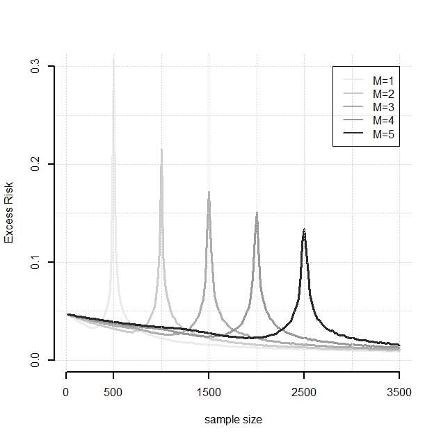
Figure 3: Double descent for MSDYear dataset from Section 6 with $d=90$ features. We observe peaks whenever $d=\frac{n}{M}$, as Theorem B.6 predicts.

Simulated Data.

In a final experiment we investigate the effect of decay of the eigenvalues on the (normalized) relative prediction efficiency, defined in Definition 4.1. We generate $n=200$ i.i.d. training points $x_{j}\sim{\mathcal{N}}(0,\Sigma)$, with $d=400$, $\lambda_{j}(\Sigma)=j^{-(1+\varepsilon)}$, with $\varepsilon=0.1,0.5,1,1.5$. The target $\beta^{*}$ is simulated according to Assumption 3.12 with ${\rm SNR}=1$. As expected from our main results, faster decay (larger $\varepsilon$) allows larger parallelization, that is, the optimal number of splits (largest efficiency) increases with faster decay.

  

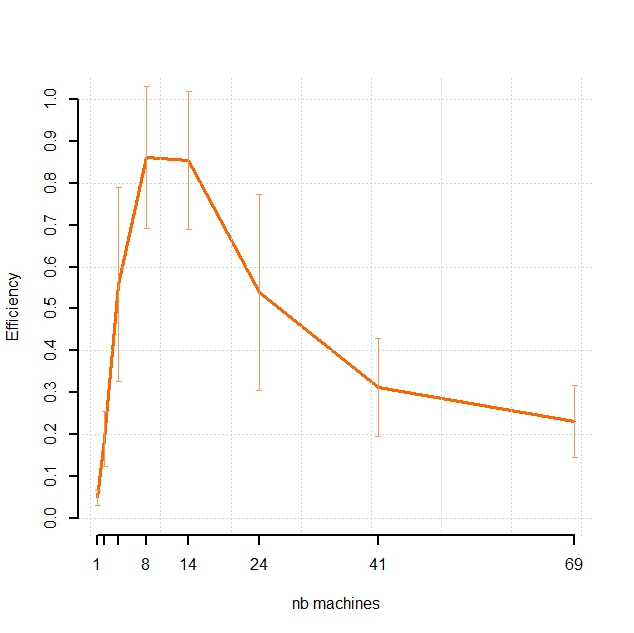
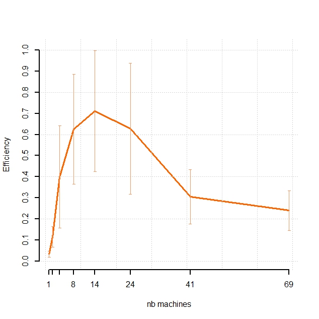
Figure 4: Left: $\varepsilon=0.1$ Right: $\varepsilon=0.5$.

  

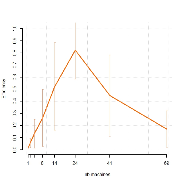
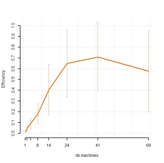
Figure 5: Left: $\varepsilon=1$ Right: $\varepsilon=1.5$.

References

• [BBL11] Ron Bekkerman, Mikhail Bilenko, and John Langford. Scaling up machine learning: Parallel and distributed approaches. Cambridge University Press, 2011.
• [Bel21] Mikhail Belkin. Fit without fear: remarkable mathematical phenomena of deep learning through the prism of interpolation. arXiv e-prints, pages arXiv–2105, 2021.
• [BFL+18] Heather Battey, Jianqing Fan, Han Liu, Junwei Lu, and Ziwei Zhu. Distributed testing and estimation under sparse high dimensional models. Annals of statistics, 46(3):1352, 2018.
• [BLLT20] Peter L Bartlett, Philip M Long, Gábor Lugosi, and Alexander Tsigler. Benign overfitting in linear regression. Proceedings of the National Academy of Sciences, 2020.
• [BM18] Gilles Blanchard and Nicole Mücke. Optimal rates for regularization of statistical inverse learning problems. Foundations of Computational Mathematics, 18(4):971–1013, 2018.
• [BMEL+] Thierry Bertin-Mahieux, Daniel PW Ellis, EE LabROSA, Brian Whitman, and Paul Lamere. The million song dataset.
• [BMR21] Peter L Bartlett, Andrea Montanari, and Alexander Rakhlin. Deep learning: a statistical viewpoint. arXiv preprint arXiv:2103.09177, 2021.
• [BPR07] Frank Bauer, Sergei Pereverzev, and Lorenzo Rosasco. On regularization algorithms in learning theory. Journal of complexity, 23(1):52–72, 2007.
• [BX21] Yajie Bao and Weijia Xiong. One-round communication efficient distributed m-estimation. In International Conference on Artificial Intelligence and Statistics, pages 46–54. PMLR, 2021.
• [CL20] Geoffrey Chinot and Matthieu Lerasle. Benign overfitting in the large deviation regime. arXiv e-prints, pages arXiv–2003, 2020.
• [CLZ17] Xiangyu Chang, Shao-Bo Lin, and Ding-Xuan Zhou. Distributed semi-supervised learning with kernel ridge regression. The Journal of Machine Learning Research, 18(1):1493–1514, 2017.
• [CX14] Xueying Chen and Min-ge Xie. A split-and-conquer approach for analysis of extraordinarily large data. Statistica Sinica, pages 1655–1684, 2014.
• [DE17] Lee H Dicker and Murat A Erdogdu. Flexible results for quadratic forms with applications to variance components estimation. The Annals of Statistics, 45(1):386–414, 2017.
• [DS21] Edgar Dobriban and Yue Sheng. Distributed linear regression by averaging. The Annals of Statistics, 49(2):918–943, 2021.
• [DW18] Edgar Dobriban and Stefan Wager. High-dimensional asymptotics of prediction: Ridge regression and classification. The Annals of Statistics, 46(1):247–279, 2018.
• [EHN96] Heinz Werner Engl, Martin Hanke, and Andreas Neubauer. Regularization of inverse problems, volume 375. Springer Science & Business Media, 1996.
• [FGW21] Jianqing Fan, Yongyi Guo, and Kaizheng Wang. Communication-efficient accurate statistical estimation. Journal of the American Statistical Association, pages 1–11, 2021.
• [FWWZ19] Jianqing Fan, Dong Wang, Kaizheng Wang, and Ziwei Zhu. Distributed estimation of principal eigenspaces. Annals of statistics, 47(6):3009, 2019.
• [GLW+21] Yuan Gao, Weidong Liu, Hansheng Wang, Xiaozhou Wang, Yibo Yan, and Riquan Zhang. A review of distributed statistical inference. Statistical Theory and Related Fields, pages 1–11, 2021.
• [GLZ17] Zheng-Chu Guo, Shao-Bo Lin, and Ding-Xuan Zhou. Learning theory of distributed spectral algorithms. Inverse Problems, 33(7):074009, 2017.
• [Hol20] David Holzmüller. On the universality of the double descent peak in ridgeless regression. stat, 1050:5, 2020.
• [KL17] Vladimir Koltchinskii and Karim Lounici. Concentration inequalities and moment bounds for sample covariance operators. Bernoulli, 23(1):110–133, 2017.
• [LC18] Junhong Lin and Volkan Cevher. Optimal distributed learning with multi-pass stochastic gradient methods. In International Conference on Machine Learning, pages 3092–3101. PMLR, 2018.
• [LGZ17] Shao-Bo Lin, Xin Guo, and Ding-Xuan Zhou. Distributed learning with regularized least squares. The Journal of Machine Learning Research, 18(1):3202–3232, 2017.
• [LRRC20] Junhong Lin, Alessandro Rudi, Lorenzo Rosasco, and Volkan Cevher. Optimal rates for spectral algorithms with least-squares regression over hilbert spaces. Applied and Computational Harmonic Analysis, 48(3):868–890, 2020.
• [LZ18] Shao-Bo Lin and Ding-Xuan Zhou. Distributed kernel-based gradient descent algorithms. Constructive Approximation, 47(2):249–276, 2018.
• [MB18] Nicole Mücke and Gilles Blanchard. Parallelizing spectrally regularized kernel algorithms. The Journal of Machine Learning Research, 19(1):1069–1097, 2018.
• [MMM+09] Gideon Mann, Ryan McDonald, Mehryar Mohri, Nathan Silberman, and Daniel D Walker. Efficient large-scale distributed training of conditional maximum entropy models. In Proceedings of the 22nd International Conference on Neural Information Processing Systems, pages 1231–1239, 2009.
• [MNR19] Nicole Mücke, Gergely Neu, and Lorenzo Rosasco. Beating sgd saturation with tail-averaging and minibatching. In Advances in Neural Information Processing Systems, pages 12568–12577, 2019.
• [MP03] Peter Mathé and Sergei V Pereverzev. Geometry of linear ill-posed problems in variable hilbert scales. Inverse problems, 19(3):789, 2003.
• [MTJ11] Lester Mackey, Ameet Talwalkar, and Michael I Jordan. Divide-and-conquer matrix factorization. Advances in neural information processing systems, 24, 2011.
• [MVSS20] Vidya Muthukumar, Kailas Vodrahalli, Vignesh Subramanian, and Anant Sahai. Harmless interpolation of noisy data in regression. IEEE Journal on Selected Areas in Information Theory, 1(1):67–83, 2020.
• [NDR20] Jeffrey Negrea, Gintare Karolina Dziugaite, and Daniel Roy. In defense of uniform convergence: Generalization via derandomization with an application to interpolating predictors. In International Conference on Machine Learning, pages 7263–7272. PMLR, 2020.
• [PG19] Stephen Page and Steffen Grünewälder. Ivanov-regularised least-squares estimators over large rkhss and their interpolation spaces. J. Mach. Learn. Res., 20:120–1, 2019.
• [Ree12] Michael Reed. Methods of modern mathematical physics: Functional analysis. Elsevier, 2012.
• [RMR20] Dominic Richards, Jaouad Mourtada, and Lorenzo Rosasco. Asymptotics of ridge (less) regression under general source condition. arXiv preprint arXiv:2006.06386, 2020.
• [RN16] Jonathan D Rosenblatt and Boaz Nadler. On the optimality of averaging in distributed statistical learning. Information and Inference: A Journal of the IMA, 5(4):379–404, 2016.
• [RV15] Lorenzo Rosasco and Silvia Villa. Learning with incremental iterative regularization. Advances in Neural Information Processing Systems 28, pages 1630–1638, 2015.
• [SD20] Yue Sheng and Edgar Dobriban. One-shot distributed ridge regression in high dimensions. In International Conference on Machine Learning, pages 8763–8772. PMLR, 2020.
• [Sha21] Zong Shang. Benign overfitting without concentration, 2021.
• [SLS18] Chengchun Shi, Wenbin Lu, and Rui Song. A massive data framework for m-estimators with cubic-rate. Journal of the American Statistical Association, 113(524):1698–1709, 2018.
• [Ver18] Roman Vershynin. High-dimensional probability: An introduction with applications in data science, volume 47. Cambridge university press, 2018.
• [XSC19] Ganggang Xu, Zuofeng Shang, and Guang Cheng. Distributed generalized cross-validation for divide-and-conquer kernel ridge regression and its asymptotic optimality. Journal of computational and graphical statistics, 28(4):891–908, 2019.
• [ZDW13] Yuchen Zhang, John C Duchi, and Martin J Wainwright. Communication-efficient algorithms for statistical optimization. The Journal of Machine Learning Research, 14(1):3321–3363, 2013.
• [ZDW15] Yuchen Zhang, John Duchi, and Martin Wainwright. Divide and conquer kernel ridge regression: A distributed algorithm with minimax optimal rates. The Journal of Machine Learning Research, 16(1):3299–3340, 2015.