Multi-label Classification with Partial Annotations using Class-aware Selective Loss

Abstract

Large-scale multi-label classification datasets are commonly, and perhaps inevitably, partially annotated. That is, only a small subset of labels are annotated per sample. Different methods for handling the missing labels induce different properties on the model and impact its accuracy. In this work, we analyze the partial labeling problem, then propose a solution based on two key ideas. First, un-annotated labels should be treated selectively according to two probability quantities: the class distribution in the overall dataset and the specific label likelihood for a given data sample. We propose to estimate the class distribution using a dedicated temporary model, and we show its improved efficiency over a naïve estimation computed using the dataset’s partial annotations. Second, during the training of the target model, we emphasize the contribution of annotated labels over originally un-annotated labels by using a dedicated asymmetric loss. With our novel approach, we achieve state-of-the-art results on OpenImages dataset (e.g. reaching 87.3 mAP on V6). In addition, experiments conducted on LVIS and simulated-COCO demonstrate the effectiveness of our approach. Code is available at https://github.com/Alibaba-MIIL/PartialLabelingCSL.

1 Introduction

Recently, a remarkable progress has been made in multi-label classification [7, 29, 4, 16]. Dedicated loss functions were proposed in [2, 27], as well as transformers based approaches [16, 19, 5]. In many common cases, such as [15, 8, 6, 14, 11], as the amounts of samples and labels in the data increase, it becomes impractical to fully annotate each image. For example, OpenImages dataset [15] consists of 9 million training images and having 9,600 classes. An exhaustive annotation process would require annotating more than 86 billion labels. As a result, partially labeled data is inevitable in realistic large-scale multi-label classification tasks. A partially labeled image is annotated with a subset of positive labels and a subset of negative labels, where the rest un-annotated labels are considered as unknown (Figure 1). Typically, the majority of the labels are un-annotated. For example, on average, a picture in OpenImages is annotated with only 7 labels. Thus, the question of how to treat the numerous un-annotated labels may have a considerable impact on the learning process.

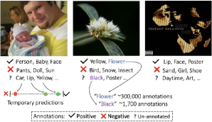
Figure 1: Challenges in partial annotation. (1) “Lip” and “Yellow” are clearly present in the left image but were not annotated as positive labels. The middle and right images are annotated with “Yellow” and “Lip” respectively, while not being dominant labels in those images. (2) The deficiency of positive annotations is a key challenge: classes that frequently appear in images (e.g. “Black”, “Lip”) may be annotated much less comparing with infrequent classes (“Flower”, “Guitar”) (3) Most labels are un-annotated. How to exploit a temporary model’s predictions for the un-annotated labels when training a target model?

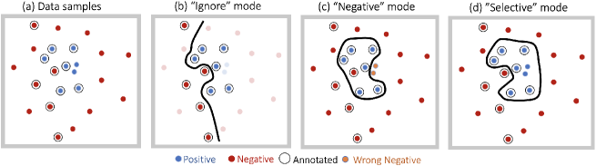
Figure 2: Illustration of training modes for handling partial labeling. (a) In a partially labeled dataset, only a portion of the samples are annotated for a given class. (b) Ignore mode exploits only a subset of the samples which may lead to a limited decision boundary. (c) Negative mode treats all un-annotated labels as negatives. It may produce suboptimal decision boundary as it adds noise of un-annotated positive labels. Also, annotated and un-annotated negative samples contribute similarly to the optimization process. (d) Our approach aims at mitigating these drawbacks by predicting the probability of a label being present in the image.

The basic training mode for handling the un-annotated labels is simply to ignore their contribution in the loss function, as proposed in [6]. We denote this mode as Ignore. While ignoring the un-annotated labels is a reasonable choice, it may lead to a poor decision boundary as it exploits only a fraction of the data, see Figure 2(b). Moreover, in a typical multi-label dataset, the probability of a label being negative is very high. Consequently, treating the un-annotated labels as negative may improve the discriminative power as it enables the exploitation of the entire data [14]. However, this training mode, denoted as Negative, has two main drawbacks: adding label noise to the training, and inducing a high imbalance between negative and positive samples [2]. This mode is illustrated in Figure 2(c).

While treating the un-annotated labels as negative can be useful for many classes, it may significantly harm the learning of labels that tend to appear frequently in the images although not being sufficiently annotated. For example, color classes are labeled in only a small number of samples in OpenImages [15], e.g. class “Black” is annotated in 1,688 samples, which is only $0.02\%$ of the samples, while they are probably present in most of the images (see an example in Figure 1). Consequently, such classes are trained with many wrong negative samples. Thus, it would be worthwhile to first identify the frequent classes in the data and treat them accordingly. While in fully annotated multi-label datasets (e.g. MS-COCO [18]) the class frequencies can be directly inferred by counting the number of their annotations, in partially annotated datasets it is not straightforward. Counting the number of positive annotations per class is misleading as the numbers are usually not proportional to the true class frequencies. In OpenImages, assumably infrequent classes like “Boat” and “Snow” are annotated in more than 100,000 samples, while frequent classes as colors are annotated in only $\sim$1,500 images. Therefore, the class distribution is required to be estimated from the data.

In this paper, we propose a Selective approach that aims at mitigating the weaknesses raised by the primary training modes (Figure 2). In particular, we will select one of the primary mode (Ignore or Negative) for each label individually by utilizing two probabilistic conditions, termed as label likelihood and label prior. The label likelihood quantifies the probability of a label being present in a specific image. The label prior represents the probability of a label being present in the data. To acquire a reliable label prior, we propose a method for estimating the class distribution. To that end, we train a classification model using Ignore mode and evaluate it on a representative dataset. Then, when training the final model, to handle the high negative-positive imbalance, we adopt the asymmetric loss [2], which enables focusing on the hard samples, while at the same time controlling the impact from the positive and negative samples. We further suggest decoupling the focusing levels of the annotated and un-annotated terms in the loss to emphasize the contributions from the annotated negative samples.

Extensive experiments were conducted on three datasets: OpenImages [15] (V3 and V6) and LVIS [8] which are partially annotated datasets with 9,600 and 1,203 classes, respectively. In addition, we simulated partially annotated versions of the MS-COCO [18] for exploring and verifying our approach. Results and comparisons demonstrate the effectiveness of our proposed scheme. Specifically, on OpenImages (V6) we achieve a state-of-the-art result of $87.34\%$ mAP score. The contributions of the paper can be summarized as follows:

• Introducing a novel selective scheme for handling partially labeled data, that treat each un-annotated label separately based on two probabilistic quantities: label likelihood and label prior. Our approach outperforms previous methods in several partially labeled benchmarks.

• We identify a key challenge in partially labeled data, regarding the inaccuracy of calculating the class distribution using the annotations, and offer an effective approach for estimating the class distribution from the data.

• A partial asymmetric loss is proposed to dynamically control the impact of the annotated and un-annotated negative samples.

2 Related Work

Several methods had been proposed to tackle the partial labeling challenge. [6] offered a partial binary cross-entropy (CE) loss to weigh each sample according to the proportion of known labels, where the un-annotated labels are simply ignored in the loss computation. In [14] they proposed to involve also the un-annotated labels in the loss, treating them as negative while smoothing their contribution by incorporating a temperature parameter in their sigmoid function. An interactive approach was presented in [11] whose loss is composed of cross-entropy for the annotated labels and a smoothness term as a regularization. A curriculum learning strategy was also used in [6] to complete the missing labels. Instead of using the same training mode for all classes, in this paper we propose adjusting the training mode, either as Ignore or Negative for each class individually, relying on probabilistic based conditions. Also, we introduce a key challenge in partial labeling, concerning the inability to infer the class distribution directly from the number of annotations, and suggest an estimation procedure to handle this.

Other methods were proposed in [30, 28, 26] to cope with partial labels, for example by a low-rank empirical risk minimization [30] or by learning structured semantic correlations [28]. However, they are not scalable to large datasets and their optimization procedures are not well adapted to deep neural networks.

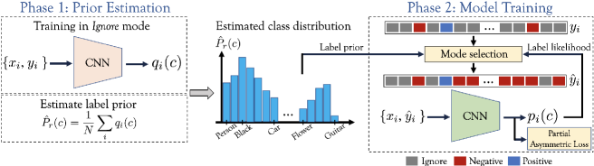
Figure 3: Proposed approach. First, a class distribution estimation phase is performed to obtain a reliable label prior using a temporary network trained with the Ignore mode. Then, the target model is trained using a Selective approach which assigns a Negative or Ignore mode for each label based on its estimated prior and likelihood.

Positive Unlabeled (PU) is also related to partial labeling [1, 12, 9]. The difference is that PU learning approaches use only positive and un-annotated labels without any negative annotations.

3 Learning from Partial Annotations

3.1 Problem Formulation

Given a partially annotated multi-label dataset with $C$ classes, each sample $\mathbf{x}\in\mathcal{X}$, corresponding to a specific image, and is annotated by a label vector $\mathbf{y}=\{y_{c}\}_{c=1}^{C}$, where $y_{c}\in\{-1,0,1\}$ denotes whether the class $c$ is present in the image (‘$1$’), absent (‘$-1$’) or unknown (‘$0$’). For a given image, we denote the sets of positive and negative labels as $\mathcal{P}_{\mathbf{x}}=\{c|y_{c}=1\}$, and $\mathcal{N}_{\mathbf{x}}=\{c|y_{c}=-1\}$, respectively. The set of un-annotated labels is denoted by $\mathcal{U}_{\mathbf{x}}=\{c|y_{c}=0\}$. Note that typically, $|\mathcal{P}_{\mathbf{x}}\cup\mathcal{N}_{\mathbf{x}}|\ll|\mathcal{U}_{\mathbf{x}}|$. A general form of the partially annotated multi-label classification loss can be defined as follows,

$$\mathcal{L}(\mathbf{x})=\sum_{c\in\mathcal{P}_{\mathbf{x}}}\mathcal{L}_{c}^{+}(\mathbf{x})+\sum_{c\in\mathcal{N}_{\mathbf{x}}}\mathcal{L}_{c}^{-}(\mathbf{x})+\sum_{c\in\mathcal{U}_{\mathbf{x}}}\mathcal{L}_{c}^{u}(\mathbf{x})$$ (1)

where $\mathcal{L}_{c}^{+}(\mathbf{x})$, $\mathcal{L}_{c}^{-}(\mathbf{x})$ and $\mathcal{L}_{c}^{u}(\mathbf{x})$ are the loss terms of the positive, negative and un-annotated labels for sample $\mathbf{x}$, respectively. Given a set of $N$ labeled samples $\{\mathbf{x}_{i},\mathbf{y}_{i}\}_{i=1}^{N}$, our goal is to train a neural-network model $f(\mathbf{x};\boldsymbol{\theta})$, parametrized by $\boldsymbol{\theta}$, to predict the presence or absence of each class given an input image. We denote by $\mathbf{p}=\{p_{c}\}_{c=1}^{C}$ the class prediction vector, computed by the model: $p_{c}=\sigma(z_{c})$ where $\sigma(\cdot)$ is the sigmoid function, and $z_{c}$ is the output logit corresponding to class $c$.

For example, applying the binary CE loss while considering only the annotated labels is defined by setting the loss terms as $\mathcal{L}_{c}^{+}(\mathbf{x})=\log(p_{c})$, $\mathcal{L}_{c}^{-}(\mathbf{x})=\log(1-p_{c})$ and $\mathcal{L}_{c}^{u}(\mathbf{x})=0$.

3.2 How to Treat the Un-annotated Labels?

Typically, the number of un-annotated labels is much higher than the annotated ones. Therefore, the question of how to treat the un-annotated labels may have a considerable impact on the learning process. Herein, we will first define the two primary training modes and detail their strengths and limitations. Then, in light of these insights, we will propose a class aware mechanism which may better handle the un-annotated labels.

Mode Ignore. The basic scheme for handling the un-annotated labels is simply to ignore them, as suggested in [6]. In this mode we set $\mathcal{L}_{c}^{u}(\mathbf{x})=0$. This way the training data is not contaminated with wrong annotations. However, its drawback is that it enables to use only a subset of the data. For example, in OpenImages dataset, the number of samples with either positive or negative annotations for the class “Cat” is only $\sim 0.9\%$ of the training data. This may lead to a sub-optimal classification boundary when the annotated negative labels do not sufficiently cover the space of the negative class. See illustration in Figure 2(b).

Mode Negative. In typical multi-label datasets, the chance of a specific label to appear in an image is very low. For example, in the fully-annotated MS-COCO dataset [18], a label is annotated as negative with a probability of $\sim 0.96$. Based on this prior assumption, a reasonable choice would be to treat the un-annotated labels as negative, i.e. setting $\mathcal{L}_{c}^{u}(\mathbf{x})=\mathcal{L}_{c}^{-}(\mathbf{x})$. This working mode was also suggested in [14]. While this mode enables the utilization of the entire dataset, it suffers from two main limitations. First, it may wrongly annotate positive labels as negative annotations, adding label noise to the training. Secondly, this mode inherently triggers a high imbalance between negative and positive samples. Balancing them, for example by down-weighting the contribution of the negative samples, may diminish the impact of the valuable annotated negative samples. These weaknesses are illustrated in Figure 2(c).

The question of which mode to choose has no unequivocal answer. It depends on various conditions and may have its origin in the annotation scheme used. In section 5.1, we will show that different partial annotation procedures can lead to favor different loss modes (See Figure 6). Moreover, as discussed in the next section, the used mode can influence each class differently, depends upon the class presence frequency in the data and the number of available annotations.

3.3 Class Distribution in Partial Annotation

As aforementioned, in multi-label datasets the majority of labels are present in only a small fraction of the data. For example, in MS-COCO, $89\%$ of the classes appear in less than $5\%$ of the data. Thus, treating all un-annotated labels as negative may improve the discriminative power for many classes, as more real negative samples are involved in the training, while the added label noise is negligible. However, this may significantly harm the learning of classes whose number of positive annotations in the dataset is much lower than the actual number of samples they appear in. Consider the case of the class “Person” in MS-COCO. It is present in $55\%$ of the data (45,200 samples). Now, suppose that only a subset of 1,000 positive annotations are available, and the rest are switched to negative. It means that during the training, most of the prediction errors are due to wrong annotations. In this case, the optimization will be degraded and the network confidence will be decayed considerably. Hence, it will be beneficial to first identify the frequent labels and handle them differently in the loss.

3.3.1 Positive Annotations Deficiency

To identify the frequent labels, we need to reliably acquire their distribution in the data. While in fully annotated datasets it can be easily obtained by counting the number of annotations per class and normalizing by the total number of samples, in partially annotated datasets it is not straightforward. While one may suggest counting the number of positive annotations for each class, the resulted numbers are misleading and are usually not proportional to the true class frequencies. For example, in OpenImages (V6), we found that many common and general classes which are frequently present in images are labeled with very few positive annotations. For example, general classes such as “Daytime”, “Event” or “Design” are labeled in only 1,709, 1,517 and 1,394 images (out of 9M), respectively. Color classes which massively appear in images are also rarely annotated. “Black” and “White” classes are labeled in only 1,688 and 1,497 images, respectively. We may assume that classes such as “Daytime” or “White” are present in much more than $0.02\%$ of the samples. Similarly, in LVIS dataset, the classes “Person” and “Shirt” are annotated in only 1,928 and 1,942 samples, respectively, while they practically appear in much more images (note that in MS-COCO, which shares the same images with LVIS, the class “Person” appears in $55\%$ of the samples).

Note that the labels are not necessarily annotated according to their dominance in the image. In Figure 1, we show examples of three images and corresponding annotations of the classes “Lip” and “Yellow”. As can be seen, the left image was not annotated with neither “Lip” nor “Yellow” although these labels are present and dominant in it. Also, “Lip” is annotated in only 1,121 images which is highly deficient in view of the fact that the class “Human face” is annotated in 327,899 images.

According to the above-mentioned observations, the number of positive annotations cannot be used to measure the class frequencies in partially labeled datasets. In section 4.2, we will propose a simple yet effective approach for estimating the class distribution from the data.

4 Proposed Approach

In this section we will present our method which aims at mitigating the issues raised in training partially annotated data. An overview of the proposed approach is summarized in Figure 3.

To mitigate the high negative-positive imbalance problem, we adopt the asymmetric loss (ASL) proposed in [2] as the base loss for the multi-label classification task. It enables to dynamically focus on the hard samples while at the same time controlling the contribution propagated from the positive and negative samples. First, let us denote the basic term of the focal loss [17] for a given class $c$, by:

$$\mathcal{L}_{\scaleto{F}{3.5pt}}(p_{c},\gamma)=(1-p_{c})^{\gamma}\log p_{c}$$ (2)

where $\gamma$ is the focusing parameter, which adjusts the decay rate of the easy samples. Then, we define the partially annotated loss as follows,

$$\begin{split}\mathcal{L}(\mathbf{x})&=\smashoperator[lr]{\sum_{c\in\mathcal{P}_{\mathbf{x}}}^{}}\mathcal{L}_{\scaleto{F}{3.5pt}}(p_{c},\gamma^{+})\\ &+\smashoperator[lr]{\sum_{c\in\mathcal{N}_{\mathbf{x}}}^{}}\mathcal{L}_{\scaleto{F}{3.5pt}}(1-p_{c},\gamma^{-})+\smashoperator[lr]{\sum_{c\in\mathcal{U}_{\mathbf{x}}}^{}}\omega_{c}\mathcal{L}_{\scaleto{F}{3.5pt}}(1-p_{c},\gamma^{u})\end{split}$$ (3)

where $\gamma^{+}$, $\gamma^{-}$ and $\gamma^{u}$ are the focusing parameters for the positive, negative and un-annotated labels, respectively. $\omega_{c}$ is the selectivity parameter and it is introduced in section 4.1. We usually set $\gamma^{+}<\gamma^{-}$ to decay the positive term with a lower rate than the negative one because the positive samples are infrequent compared to the negative samples. In addition, as for a given class, the negative annotated samples are verified ground-truth we are interested in preserving their contribution to the loss. Therefore, we suggest decoupling of the focusing parameter of the annotated negative labels from the un-annotated one, allowing us to set a lower decay rate for the annotated negative labels: $\gamma^{-}<\gamma^{u}$. This way, the impact of the annotated negative samples on establishing the classification boundary for each class is higher (see Figure 2(d)). We term this form of asymmetric loss as Partial-ASL (P-ASL).

4.1 Class-aware Selective Loss

As described in section 3.1, both Ignore and Negative modes are supported by inadequate assumptions for the partial annotation problem. In this section, we propose a selective approach for adjusting the mode per individual class. The core idea is to examine the probability of each un-annotated label being present in a given sample $\mathbf{x}$. Un-annotated labels that are suspected as positive will be ignored. The others will be treated as negative.

For that purpose, we define two probabilistic values: label likelihood and label prior, and detail their usage in the following section. These two quantities are complementary to each other. The label likelihood enables to dynamically ignore the loss contribution of a label in a given image by inspecting its visual content. The label prior extracts useful information of the estimated class frequencies in the data and uses it regardless of the specific image content.

Label likelihood. Defined by the conditional probability of an un-annotated label $c$ of being positive given the image and the model parameters. i.e.

$$P(y_{c}=1|\mathbf{x};\boldsymbol{\theta});\quad\forall c\in\mathcal{U}_{\mathbf{x}}$$ (4)

It can be simply estimated by the network prediction $\{p_{c}\}_{c\in\mathcal{U}_{\mathbf{x}}}$ throughout the training. A high $p_{c}$ may imply that the un-annotated label $c$ appears in the image, and treating it as negative may lead to an error. Accordingly, the label $c$ should be ignored. In practice, we allow for $K$ un-annotated labels with top prediction values to be ignored. i.e.

$$\Omega_{L}=\big{\{}c\in\mathcal{U}_{\mathbf{x}}\mid c\in\text{TopK}(\{p_{c}\})\big{\}}$$ (5)

where the $\text{TopK}(\cdot)$ operator returns the indices of the top $K$ elements of the input vector. The algorithm scheme is illustrated in Figure 4. Note that this implementation enables us to “walk” on a continuous scale between the Negative and Ignore modes. Setting $K=0$ corresponds to Negative mode, as no un-annotated label is ignored. $K=C$ equivalents to the Ignore mode, as all un-annotated labels are ignored.

Label prior. Defined by the probability of a label $c$ being present in an image. It can also be viewed as the actual label presence frequency in the data. We are interested in the label prior for the un-annotated labels,

$$P(y_{c}=1);\quad\forall c\in\mathcal{U}_{\mathbf{x}}.$$ (6)

According to section 3.3, the label prior should be estimated from the data, as the class distribution is hidden in partially annotated datasets. In the next section (4.2), we will introduce the scheme for estimating the label prior. Meanwhile, let us denote by $\hat{P}_{r}(c)$ the label prior estimator for class $c$. We are interested in disabling the loss contribution of labels with high prior values. These labels are formally defined by the following set,

$$\Omega_{P}=\big{\{}c\in\mathcal{U}_{\mathbf{x}}\mid\hat{P}_{r}(c)>\eta\big{\}}$$ (7)

where $\eta\in[0,1]$ represents the minimum fraction of the data determining a label to be ignored.

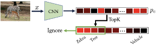
Figure 4: Using the label likelihood. Un-annotated labels with highest network confidence may be related to positive items in the image. Thus, we ignore them in the loss computation.

Finally, we denote the set of labels whose loss contribution are ignored, as the union of the two previously computed sets,

$$\Omega_{\text{Ignore}}=\Omega_{L}\cup\Omega_{P}.$$ (8)

Accordingly, we set the parameter $\omega_{c}$ in equation (3) as follows,

$$\omega_{c}=\begin{cases}0\quad c\in\Omega_{\text{Ignore}}\\ 1\quad c\notin\Omega_{\text{Ignore}}\\ \end{cases}$$ (9)

Note that we have explored other alternatives for implementing the label prior in the loss function. In particular, in appendix B we compare a soft method that integrates the label prior by setting $\omega_{c}=\exp(-\alpha\hat{P}_{r}(c));\forall c\notin\Omega_{L}$, and show that using a hard decision mechanism, as proposed in equation (9), produces better results.

4.2 Estimating the Class Distribution

We aim at estimating the class distribution in a representative dataset $\mathcal{X}$. For that, we first need to assess the presence of each class in every image in the data, i.e. we would like to first approximate the probability of a class $c$ being present in an image $\mathbf{x}\in\mathcal{X}$: $P(y_{c}=1|\mathbf{x})$. To that end, we propose training a model parametrized by $\boldsymbol{\theta}$, for predicting each class in a given image, i.e. $P(y_{c}=1|\mathbf{x};\boldsymbol{\theta})$. Afterwards, the model is applied on the sample set $\mathcal{X}$ (e.g. the training data). The label prior can then be estimated by calculating the expectation,

$$\vspace{-0.15cm}P(y_{c}=1;\mathbf{\theta})=\frac{1}{|\mathcal{X}|}\sum_{\mathbf{x}\in\mathcal{X}}P(y_{c}=1|\mathbf{x};\boldsymbol{\theta}).\vspace{-0.1cm}$$ (10)

For estimating the label priors, we train the model in Ignore mode. While the discriminative power of the Negative mode may be stronger for majority of the labels, it may fail to provide a reliable prediction values for frequent classes with small number of positive annotations. Propagating abundance of gradient errors from wrong negative annotations will decay the expected returned prediction for those classes and will fail to approximate $P(y_{c}=1|\mathbf{x})$. Consequently, our suggested estimation for the class distribution is given by,

$$\hat{P}_{r}(c)=P(y_{c}=1;\mathbf{\boldsymbol{\theta}_{\text{Ignore}}}),$$ (11)

where $\boldsymbol{\theta}_{\text{Ignore}}$ denotes the model parameters trained in Ignore mode. In section 5.2, we will empirically show the effectiveness of the Ignore mode in ranking the class frequencies and the inapplicability of the Negative mode to do that. To qualitatively show the estimation effectiveness, we present in Figure 5 the top 20 frequent classes in OpenImages (V6) as estimated by our proposed procedure. Note that all the top classes are commonly present in images such as colors (“White”, “Black”, “Blue” etc.) or general classes such as “Photograph”, “Light”, “Daytime” or “Line”. In appendix D, we show the next top 60 estimated classes. Also, in appendix E, we provides the top 20 estimated frequent classes for LVIS dataset.

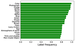
Figure 5: Estimating the class distribution in OpenImages. Top 20 frequent classes estimated by the Ignore model. Top classes are all related to common labels such as colors or general concepts.

5 Experimental Study

In this section, we will experimentally demonstrate the insights discussed in the previous sections. We will mainly utilize the fully annotated MS-COCO dataset [18] to validate and demonstrate the effectiveness of our approach by simulating partial annotation under specific case studies. The evaluation metric used in the experiments is the mean average precision (mAP). Training details are provided in appendix A.

5.1 Impact of Annotation Schemes

As aforementioned in section 3.2, the scheme used for annotating the dataset can substantially induce the learning process. Specifically, the choice of how to treat the un-annotated labels is highly influenced by the annotation scheme. To demonstrate that, we simulate two partial annotation schemes on the original fully annotated MS-COCO dataset [18]. MS-COCO includes 80 classes, 82,081 training samples, and 40,137 validation samples, following the 2014 split. The two simulated annotation schemes are detailed as follows:

Fixed per class (FPC). For each class, we randomly sample a fixed number of positive annotations, denoted by $N_{s}$, and the same number of negative annotations. The rest of the annotations are dropped.

Random per annotation (RPA). We omit each annotation with probability $p$. Note that this simulation preserves the true class distribution of the data.

In Figure 6, we show results obtained using each one of the simulation schemes for each primary mode (Ignore and Negative) while varying $N_{s}$ and $p$ values. As can be seen, while in RPA (Figure 6(a)), the Ignore mode consistently shows better results, in FPC (Figure 6(b)), the Negative mode is superior. Note that as we keep more of the annotated labels (by either increasing $N_{s}$ or decreasing $p$), the gap between the two training modes is reduced, catching the maximal result. The phenomenons observed in the two case studies we simulated are also related in real practical procedures for partially annotating multi-label datasets. While in the FPC simulation, the class distribution is completely vanished and cannot be inferred by the number of positive annotations ($N_{s}$ for $c=1,...,C$), the RPA scheme preserves the class distribution.

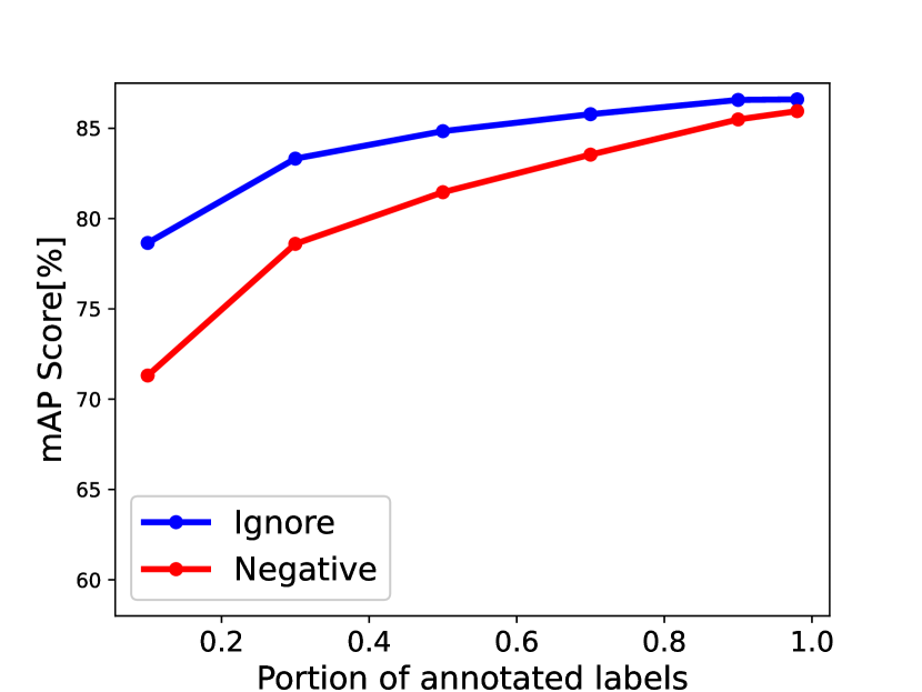
(a)

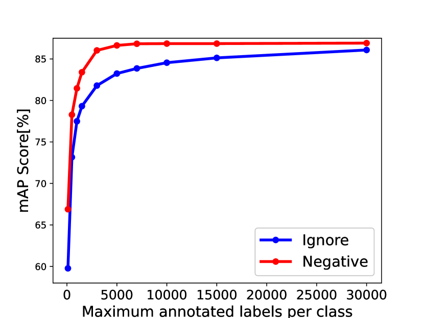
(b)

Figure 6: Impact of annotation schemes. mAP results obtained using the RPA (a) and the FPC (b) simulation schemes for each primary mode. While in RPA, Ignore mode consistently shows better results, in FPC, the Negative mode is superior.

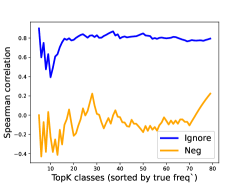
Figure 7: Spearman correlation between the true class distribution and the estimated distribution. Unlike the Negative mode, training a model using Ignore mode is well suited for estimating the class distribution.

5.2 Estimating the Label Prior

To demonstrate the estimation quality of the class distribution obtained by the approach proposed in section 4.2, we follow the FPC simulation scheme applied on the MS-COCO dataset (as described in section 5.1), where a constant number of 1,000 annotations remained for each class. Because MS-COCO is a fully annotated dataset, we can compare the estimated class distribution (i.e. the label prior) to the true class distribution inferred by the original number of annotations. In particular, we measure the similarity between the original class frequencies and the estimated ones using the Spearman correlation test. In figure 7, we show the Spearman correlation scores while varying the number of top-ranked classes. We also show the results obtained with Negative mode as a reference. Specifically, the Spearman correlation computed over all the 80 classes, with the estimator obtained using the Ignore mode is $0.81$, demonstrating the estimator’s effectiveness. In the next section, we will show how it benefits the overall classification results. Also, in appendix C we present the top frequent classes measured by our estimator and compare them to those obtained by the original class frequencies in MS-COCO.

6 Benchmark Results

In this section, we will report our main results on the partially annotated multi-label datasets: OpenImages [15], and LVIS [8]. The results on MS-COCO dataset are presented in appendix C. We will present a comparison to previous methods which handle partial annotations, among other baseline approaches in multi-label classification. The evaluation metric used in the experiments is the mean average precision (mAP). In particular, we report the standard per-class mAP denoted as mAP(C), and overall mAP denoted as mAP(O), which considers the number of samples in each class. The training details and the loss hyper-parameters used are provided in appendix A.

Method	mAP(C)	mAP(O)
CE, Ignore	85.38	93.15
wCE [6], Ignore	85.22	93.05
CE, Negative	85.35	91.14
SE(LS) [14], Negative	85.70	91.20
ASL [2], Negative	85.85	91.29
P-ASL, Negative	86.28	92.34
P-ASL, Selective ($\Omega_{L}$)	86.36	93.25
P-ASL, Selective ($\Omega_{P}$)	86.46	93.27
P-ASL, Selective ($\Omega_{\text{Ignore}}$)	86.72	93.57

Table 1: OpenImages (V6) results. The Selective approach with P-ASL improves both mAP(C) and mAP(O) scores.

Backbone	mAP(C)	mAP(O)
OFA-595 [3]	85.40	92.87
ResNet-50 [10]	86.15	93.16
TResNet-M [23]	86.72	93.57
TResNet-L [23]	87.34	93.77

Table 2: OpenImages (V6) results for different backbones. Using TResNet-L model we achieve top results on OpenImages V6.

Method	Group 1	Group 2	Group 3	Group 4	Group 5	All classes
Latent Noise (visual) [21]	69.37	70.41	74.79	79.20	85.51	75.86
CNN-RNN [25]	68.76	69.70	74.18	78.52	84.61	75.16
Curriculum Labeling [6]	70.37	71.32	76.23	80.54	86.81	77.05
IMCL [11]	70.95	72.59	77.64	81.83	87.34	78.07
P-ASL, Selective (ours)	73.19	78.61	85.11	87.70	90.61	83.03

Table 3: Results for OpenImages (V3). Comparing the mAP score obtained using our Selective approach to previous multi-label classification methods.

6.1 OpenImages V6

Openimages V6 is a large-scale multi-label dataset [15], consists of 9 million training images, 41,620 validation samples, and 125,456 test samples. It is a partially annotated dataset, with 9,600 trainable classes. In Table 1, we present the mAP results obtained by our proposed Selective method and compare them to other approaches. Interestingly, Ignore mode produces better results than Negative mode, as OpenImages contains many under-annotated frequent classes such as colors and other general classes (see Figure 5). Using Negative mode adds a massive label noise and harms the learning of many common classes. In Table 2, we present results for different network architectures. Specifically, using TResNet-L [23], we achieve state-of-the-art result of $87.34$ mAP score.

To show the impact of decoupling the focusing parameters of the annotated and un-annotated loss terms in P-ASL as proposed in equation (3), we varied the negative focusing parameter $\gamma_{-}$, while fixing $\gamma_{u}=7$. The results are presented in Figure 8. The case of $\gamma_{-}=7$ represents the standard ASL [2]. As can be seen, the mAP score increases as we lower $\gamma_{-}$, up to 2. It indicates that lowering the decay rate for the annotated negative term boosts their contribution to the loss.

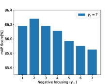
Figure 8: Impact of decoupling the focusing parameters. We set the un-annotated focusing to $\gamma_{u}=7$ and varied the annotated negative focusing $\gamma_{-}$.

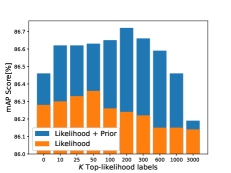
Figure 9: Ablation study of the Selective approach components. mAP results are shown for different numbers of top likelihood labels, $K$. We show results for the case of using only the likelihood condition $\Omega_{L}$, and with both conditions $\Omega_{L}\cup\Omega_{P}$.

In Figure 9, we show the mAP scores while varying the number of top likelihood classes, $K$ as defined in equation (5). Note that setting $K=0$ is equivalent to use Negative mode. Training with high enough $K$ becomes similar to training using Ignore mode. The highest mAP results are obtained with both the likelihood and prior conditions.

6.2 OpenImages V3

To be compatible with previously published results, we used the OpenImages V3 which contains 5,000 trainable classes. We follow the comparison setting described in [11]. Also, for a fair comparison we used the ResNet-101 [10] backbone, pre-trained on the ImageNet dataset. In Table 3, we show the mAP score results obtained using previous approaches and compared them to our Selective method. As shown, our method significantly outperforms previous approaches that deal with partial annotation in a multi-label setting.

6.3 LVIS

LVIS is a partially labeled dataset originally annotated for object detection and image segmentation, that was adopted as a multi-label classification benchmark. It consists of 100,170 images for training and 19,822 images for testing. It contains 1,203 classes. In Table 4, we present a comparison between different approaches on the LVIS dataset. As can be seen, in this case, the Negative mode is better, compared to the Ignore mode. This can be related to the fact that most of the labels are related to specific objects which do no appear frequently in the images. The most frequent class is “Person”. Therefore we also added its average precision to Table 4. Note that the Ignore model better learns the class “Person” compared to the one trained with Negative mode. Using the P-ASL with the Selective mode, we were able to obtain superior mAP results as well as top average precision even for the most frequent class, “Person”.

Method	mAP(C)	mAP(O)	Person-AP
CE, Ignore	74.49	95.70	99.81
wCE [6], Ignore	74.15	95.20	99.80
CE, Negative	77.82	96.66	97.20
SE [14], Negative	77.81	96.60	97.28
ASL [2], Negative	78.32	96.77	98.43
P-ASL,Selective	78.57	96.80	99.81

Table 4: Results for LVIS. The Selective approach with P-ASL improves both mAP(C) and mAP(O) scores. Also, it provides top result for the frequent class ”Person”.

7 Conclusion

In this paper, we presented a novel technique for handling partially labeled data in multi-label classification. We observed that ignoring the un-annotated labels in the loss or treating them as negative should be determined individually for each class. We proposed a selective mechanism that uses the label likelihood computed throughout the training, and the label prior which is obtained by estimating the class distribution from the data. The un-annotated labels are further softened via a partial asymmetric loss. Extensive experiments analysis shows that our proposed approach outperforms other previous methods on partially labeled datasets, including OpenImages, LVIS, and simulated-COCO.

Appendix A Training Details

Unless stated otherwise, all experiments were conducted with the following training configuration. As a default, we used the TResNet-M model [23], pre-trained on ImageNet-21k dataset [22]. The model was fine-tuned using Adam optimizer [13] and 1-cycle cosine annealing policy [24] with a maximal learning rate of 2e-4 for training OpenImages and MS-COCO, and 6e-4 for training LVIS. We used true-weight-decay [20] of 3e-4 and standard ImageNet augmentations. For fair comparison to previously published results on OpenImages V3, we also trained a ResNet-101 model, pre-trained on ImageNet.

In the OpenImages experiments we used the following hyper-parameters: $\eta=0.05$, $K=200$, $\gamma_{u}=7$, $\gamma_{-}=2$ and $\gamma_{+}=1$. In LVIS we used: $\gamma_{u}=1$, $\gamma_{-}=0$ and $\gamma_{+}=0$.

Appendix B Soft Label Prior

Herein, we will explore a soft alternative for integrating the label prior in the loss. We follow equation (3) and define the un-annotaetd weights by

$$\omega_{c}=\exp(-\alpha\hat{P}_{r}(c))$$ (12)

where $\alpha$ is the decay factor. In Table 5 we compare the soft label prior to the configuration used in section 4.1.

Method	mAP(C)	mAP(O)
P-ASL, Selective	86.72	93.57
P-ASL, Selective (soft)	86.62	93.59

Table 5: OpenImages (V6) results using soft label prior. We used $\alpha=10$.

As the soft label prior provided with lower mAP(C) results, we did not use it in our experiments.

Appendix C Results on MS-COCO

In this section, we will present the results obtained on a partially annotated version of MS-COCO, based on the fixed per class (FPC) simulation scheme. Note that in this experiment, the class distribution measured by the number of annotations is no longer meaningful, as all classes have the same number of annotations. The mAP results, as well as the average precision (AP) scores for the class ”Person”, are presented in Figure 10. The Negative mode produces higher mAP (computed over all the classes) compared to the Ignore mode. However, as the frequent class ”Person” is present in most of the images, the Negative mode is inferior, especially in the cases of a small number of annotations. Using the Selective approach, top results can be achieved for both mAP and the person AP. In Figure 11, we show the top 10 frequent classes obtained using our procedure for estimating the class distribution as described in section 4.2, and compared them to those obtained using the original class frequencies in MS-COCO. As can be seen, most of the frequent classes measured by the original distribution are also highly ranked by our estimator.

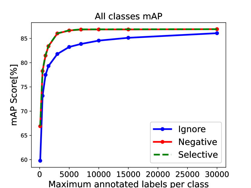
(a)

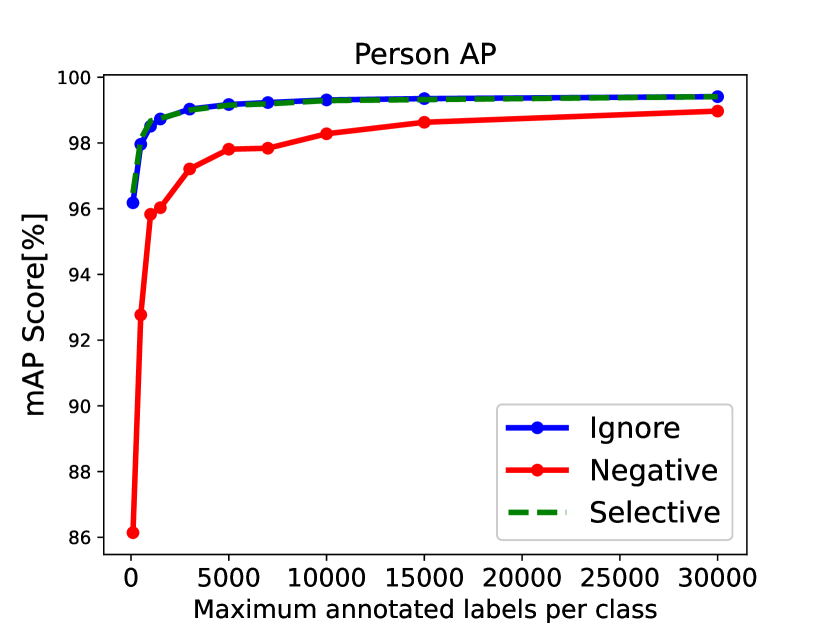
(b)

Figure 10: Results on MS-COCO (FPC). .

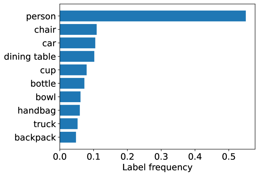
(a) Original top frequencies

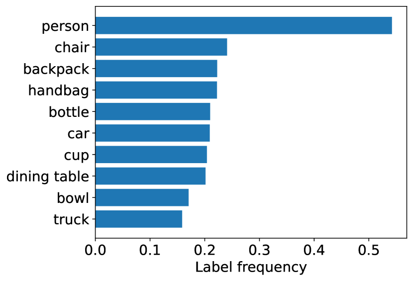
(b) Estimated top frequencies

Figure 11: Class frequency estimation in MS-COCO. Top frequent classes measured by (a) original class distribution and (b) estimated class distribution. The estimated top 10 frequent classes are included in the original top classes.

Appendix D Frequent classes in OpenImages

We add more results of the class distribution estimated by our approach (detailed in 4.2) for OpenImages dataset. See Figure 12.

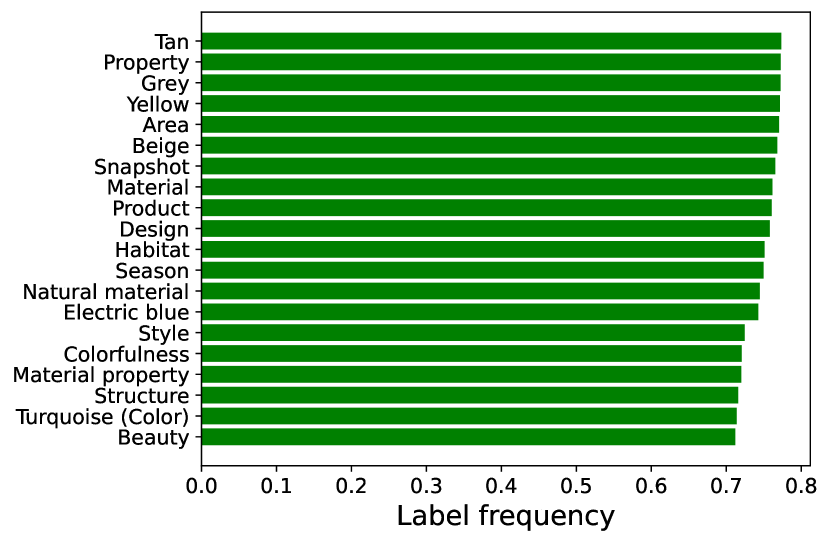
(a)

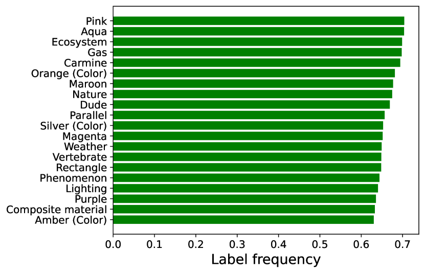
(b)

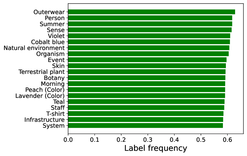
(c)

Figure 12: Estimating the calss distribution in OpenImages. Additional top 60 frequent classes as estimated by our approach.

Appendix E Frequent classes in LVIS

In Figure 13 we plot the top frequent classes in LVIS, obtained by our estimator detailed in section 4.2. Also in LVIS, it can be seen that the most estimated frequent classes are related to common objects as ”Person”, ”Shirt”, ”Trousers”, ”Shoe”, etc.

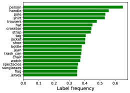
Figure 13: Estimating the calss distribution in LVIS. Top 20 frequent classes estimated by the Ignore model.

References

- [1] Jessa Bekker and Jesse Davis. Learning from positive and unlabeled data: A survey. CoRR, abs/1811.04820, 2018.
- [2] Emanuel Ben-Baruch, Tal Ridnik, Nadav Zamir, Asaf Noy, Itamar Friedman, Matan Protter, and Lihi Zelnik-Manor. Asymmetric loss for multi-label classification. arXiv preprint arXiv:2009.14119, 2020.
- [3] Han Cai, Chuang Gan, Tianzhe Wang, Zhekai Zhang, and Song Han. Once for all: Train one network and specialize it for efficient deployment. In International Conference on Learning Representations, 2020.
- [4] Zhao-Min Chen, Xiu-Shen Wei, Peng Wang, and Yanwen Guo. Multi-label image recognition with graph convolutional networks. In Proceedings of the IEEE Conference on Computer Vision and Pattern Recognition, pages 5177–5186, 2019.
- [5] Xing Cheng, Hezheng Lin, Xiangyu Wu, Fan Yang, Dong Shen, Zhongyuan Wang, Nian Shi, and Honglin Liu. Mltr: Multi-label classification with transformer, 2021.
- [6] Thibaut Durand, Nazanin Mehrasa, and Greg Mori. Learning a deep convnet for multi-label classification with partial labels. In Proceedings of the IEEE Conference on Computer Vision and Pattern Recognition, pages 647–657, 2019.
- [7] Bin-Bin Gao and Hong-Yu Zhou. Multi-label image recognition with multi-class attentional regions. arXiv preprint arXiv:2007.01755, 2020.
- [8] Agrim Gupta, Piotr Dollár, and Ross Girshick. Lvis: A dataset for large vocabulary instance segmentation, 2019.
- [9] Zayd Hammoudeh and Daniel Lowd. Learning from positive and unlabeled data with arbitrary positive shift, 2020.
- [10] Kaiming He, Xiangyu Zhang, Shaoqing Ren, and Jian Sun. Deep residual learning for image recognition. In Proceedings of the IEEE conference on computer vision and pattern recognition, pages 770–778, 2016.
- [11] D. Huynh and E. Elhamifar. Interactive multi-label CNN learning with partial labels. IEEE Conference on Computer Vision and Pattern Recognition, 2020.
- [12] Liwei Jiang, Dan Li, Qisheng Wang, Shuai Wang, and Songtao Wang. Improving positive unlabeled learning: Practical aul estimation and new training method for extremely imbalanced data sets, 2020.
- [13] Diederik P. Kingma and Jimmy Ba. Adam: A method for stochastic optimization, 2017.
- [14] Kaustav Kundu and Joseph Tighe. Exploiting weakly supervised visual patterns to learn from partial annotations. In NeurIPS, 2020.
- [15] Alina Kuznetsova, Hassan Rom, Neil Alldrin, Jasper Uijlings, Ivan Krasin, Jordi Pont-Tuset, Shahab Kamali, Stefan Popov, Matteo Malloci, Alexander Kolesnikov, and et al. The open images dataset v4. International Journal of Computer Vision, 128(7):1956–1981, Mar 2020.
- [16] Jack Lanchantin, Tianlu Wang, Vicente Ordonez, and Yanjun Qi. General multi-label image classification with transformers, 2020.
- [17] Tsung-Yi Lin, Priya Goyal, Ross B. Girshick, Kaiming He, and Piotr Dollár. Focal loss for dense object detection. CoRR, abs/1708.02002, 2017.
- [18] Tsung-Yi Lin, Michael Maire, Serge Belongie, Lubomir Bourdev, Ross Girshick, James Hays, Pietro Perona, Deva Ramanan, C. Lawrence Zitnick, and Piotr Dollár. Microsoft coco: Common objects in context, 2014.
- [19] Shilong Liu, Lei Zhang, Xiao Yang, Hang Su, and Jun Zhu. Query2label: A simple transformer way to multi-label classification, 2021.
- [20] Ilya Loshchilov and Frank Hutter. Decoupled weight decay regularization. arXiv preprint arXiv:1711.05101, 2017.
- [21] Ishan Misra, C. Lawrence Zitnick, Margaret Mitchell, and Ross Girshick. Seeing through the human reporting bias: Visual classifiers from noisy human-centric labels, 2016.
- [22] Tal Ridnik, Emanuel Ben-Baruch, Asaf Noy, and Lihi Zelnik-Manor. Imagenet-21k pretraining for the masses, 2021.
- [23] Tal Ridnik, Hussam Lawen, Asaf Noy, Emanuel Ben Baruch, Gilad Sharir, and Itamar Friedman. Tresnet: High performance gpu-dedicated architecture. In Proceedings of the IEEE/CVF Winter Conference on Applications of Computer Vision, pages 1400–1409, 2021.
- [24] Leslie N. Smith. A disciplined approach to neural network hyper-parameters: Part 1 – learning rate, batch size, momentum, and weight decay, 2018.
- [25] Jiang Wang, Yi Yang, Junhua Mao, Zhiheng Huang, Chang Huang, and Wei Xu. Cnn-rnn: A unified framework for multi-label image classification, 2016.
- [26] Baoyuan Wu, Fan Jia, Wei Liu, Bernard Ghanem, and Siwei Lyu. Multi-label learning with missing labels using mixed dependency graphs, 2018.
- [27] Tong Wu, Qingqiu Huang, Ziwei Liu, Yu Wang, and Dahua Lin. Distribution-balanced loss for multi-label classification in long-tailed datasets, 2020.
- [28] Hao Yang, Joey Tianyi Zhou, and Jianfei Cai. Improving multi-label learning with missing labels by structured semantic correlations, 2016.
- [29] Renchun You, Zhiyao Guo, Lei Cui, Xiang Long, Yingze Bao, and Shilei Wen. Cross-modality attention with semantic graph embedding for multi-label classification. In AAAI, pages 12709–12716, 2020.
- [30] Hsiang-Fu Yu, Prateek Jain, Purushottam Kar, and Inderjit S. Dhillon. Large-scale multi-label learning with missing labels, 2013.