Nulling and subpulse drifting in PSR J1727$-$2739

Abstract

In this paper, we investigate the emission properties of PSR J1727$-$2739, whose mean pulse profile has two main components, by analysing five single-pulse observations made using the Parkes 64-m radio telescope with a central frequency of 1369 MHz between 2014 April and October. The total observation time is about 6.1 hours which contains 16718 pulses after removal of radio frequency interference (RFI). Previous studies reveal that PSR J1727$-$2739 exhibits both nulling and subpulse drifting. We estimate the nulling fraction to be 66%$\pm$1.4%, which is consistent with previously published results. In addition to the previously known subpulse drifting in the leading component, we also explore the drifting properties for the trailing component. We observe two distinct drift modes whose vertical drift band separations ($P_{3}$) are consistent with earlier studies. We find that both profile components share the same drift periodicity $P_{3}$ in a certain drift mode, but the measured horizontal separations ($P_{2}$) are quite different for them. That is, PSR J1727$-$2739 is a pulsar showing both changes of drift periodicity $P_{3}$ between different drift modes and drift rate variations between components in a given drift mode. Pulsars exhibiting nulling along with drift mode changing, such as PSR J1727$-$2739, give an unique opportunity to investigate the physical mechanism of these phenomena.

1 Introduction

The radio emission of pulsars usually remains stable in intensity and polarization. However, some pulsars show remarkable emission variations, such as nulling, mode-changing, and subpulse drifting. Pulse nulling is the abrupt cessation of pulsed radio emission for a number of spin periods (Ritchings, 1976; Rankin, 1986; Wang et al., 2007; Gajjar et al., 2012). The degree of nulling in a pulsar is known as the nulling fraction (NF), which is the fraction of pulses with no detectable emission. The observed NF for nulling pulsars ranges from less than 1% to more than 95% (Wang et al., 2007; Gajjar et al., 2014; Gajjar et al., 2017; Wang et al., 2020). This phenomenon was first discovered by Backer (1970a). To date, pulse nulling has been reported in more than 200 pulsars (Wang et al., 2020). For some pulsars, their mean pulse profiles switch between two or more quasi-stable emission states. This phenomenon is referred to as mode changing. It was first observed in PSR J1239+2453 (Backer, 1970b). The typical time-scale of nulling and mode changing is several seconds to hours. In some cases, transitions between emission states are periodic. Periodic nulling has been observed in many pulsars (Herfindal & Rankin, 2007, 2009; Rankin & Wright, 2008; Rankin et al., 2013; Gajjar et al., 2014; Gajjar et al., 2017; Basu et al., 2017; Basu & Mitra, 2018; Basu et al., 2019b; Basu & Mitra, 2019). Recently, periodic mode changing also has been reported in some pulsars (Mitra & Rankin, 2017; Basu & Mitra, 2019; Yan et al., 2019, 2020).

Another well-known emission variation is subpulse drifting. Subpulse drifting is the regular phase drifting of subpulses. Since it was discovered by Drake & Craft (1968), subpulse drifting has been observed in about 120 pulsars (Weltevrede et al., 2006, 2007; Basu et al., 2016, 2019a). The drift patterns are separated horizontally across the pulse phase by $P_{2}$ (in units of degree) and vertically across time by $P_{3}$ (in units of pulse period $P_{1}$). The drift rate $\bigtriangleup\phi$ which represents the drift speed is then given by: $\bigtriangleup\phi=P_{2}/P_{3}$ (in units of °/$P_{1}$) (Smits et al., 2005; Wen et al., 2016).

Many studies reveal that nulling, mode changing and subpulse drifting may be closely linked to each other. Some pulsars show evidence of interaction between nulling and subpulse drifting. For example, the subpulse of PSR B0809+74 was found to drift more slowly after the null states (van Leeuwen et al., 2003). Janssen & van Leeuwen (2004) reported that, for PSR B0818$-$13, the subpulse drift appears to speed up during the nulls. Gajjar et al. (2017) studied the nulling–drifting interaction in PSR J1840$-$0840. They found that this pulsar tends to start nulling after the end of a drift band. Then, when the pulsar switches back on, it often starts at the beginning of a new drift band in both pulse profile components. Studies of the interaction between nulling and subpulse drifting can provide insights into the properties of pulsar magnetosphere (Redman et al., 2005; Force & Rankin, 2010). Wang et al. (2007) show clear evidence of a close relationship between nulling and mode changing. It is suggested that nulling and mode changing are different manifestations of the same physical process.

PSR J1727$-$2739 was discovered by Hobbs et al. (2004) in the Parkes Multibeam Pulsar Survey. This pulsar has a characteristic age of $1.86\times 10^{7}$ yr and a spin period of 1.29 s. It is known to show both nulling and subpulse drifting. Wen et al. (2016) studied nulling and subpulse drifting properties for PSR J1727$-$2739 using a 2-hr observation. They found that this pulsar shows nulls with lengths lasting from 6 to 281 pulses and separated by burst phases ranging from 2 to 133 pulses, and they measured a NF of 68%. Two distinct subpulse drift modes were identified, with vertical spacing between the drift bands $P_{3}$ of 9.7 $\pm$ 1.6 and 5.2 $\pm$ 0.9 pulse periods, respectively. In this paper, we carry out a detailed investigation of the single-pulse behaviour of PSR J1727$-$2739 with observations lasting for 6.1 hr. The observations and data processing are given in Section 2. Details of the results are presented in Section 3. The final conclusions and implications of our results are discussed in Section 4.

2 Observations

The observational data analysed here were downloaded from the Parkes Pulsar Data Archive that is freely available online (Hobbs et al., 2011). The observations were carried out using the Parkes 64-m radio telescope from April 1 to October 27 in 2014 at 5 epochs (see Table 1 for exact observing dates) with the center beam of the multibeam receiver (Staveley-Smith et al., 1996) and the Parkes digital filterbank systems PDFB3 and PDFB4 (Manchester et al., 2013). The total bandwidth was 256 MHz centred at 1369 MHz with 512 channels across the band. For each observation, the data were sampled every 256 $\mu$s. The total integration time is 6.1 hr for all observations.

We used the DSPSR package (van Straten & Bailes, 2011) to de-disperse and fold the data with the ephemeris from the ATNF Pulsar Catalogue V1.64 (Manchester et al., 2005). The single-pulse integrations were produced, which were recorded using the PSRFITS data format (Hotan et al., 2004) with 1024 phase bins per rotation period. Band edges (5 per cent on each side) and strong narrow-band and impulsive RFI were removed from the archive files using PAZ and PAZI programs of the PSRCHIVE packages (Hotan et al., 2004). After the RFI-excision procedure, a total of 16718 pulses were obtained from all observations. Then the RFI excised data were processed using the PSRCHIVE packages. The analysis of fluctuation spectra was performed with the PSRSALSA package (Weltevrede, 2016) which is available online. We followed Yan et al. (2011) to carry out polarization calibration using the PSRCHIVE program PAC.

3 Results

In this section, we present details of the nulling and subpulse drifting of PSR J1727$-$2739.

3.1 Nulling

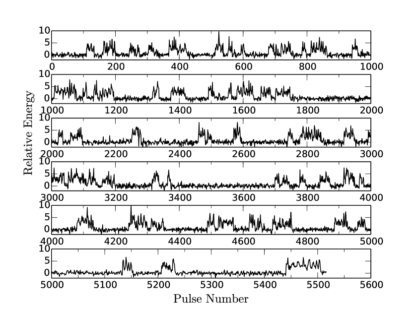
Figure 1: Pulse energy variations for the 2014-04-01 observation (see Table 1 for details). Note that pulses contaminated by RFI have been clipped. The total number of pulses displayed in this plot is 5444.

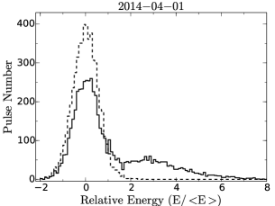
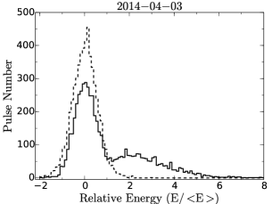
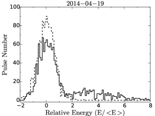
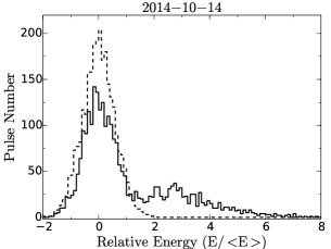
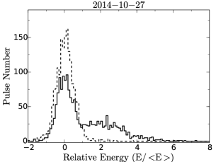
Figure 2: Pulse energy distributions for the on-pulse (solid histogram) and off-pulse (dashed histogram) regions for all observations (see Table 1 for details).

Table 1: Nulling fractions for 5 observations of PSR J1727$-$2739. Note that the symbols $\rm T_{obs}$, $\rm N_{tot}$ and $\rm N_{null}$ represent the duration, the total number of pulses and the number of null pulses of the observation, respectively. RMS_off in the last column is the mean rms of the single-pulse baseline noise.

Date	$\rm T_{obs}$	$\rm N_{tot}$	$\rm N_{null}$	NF	RMSoff
(yyyy-mm-dd)	(min)			(%)
2014-04-01	119	5444	3674	$66\pm 1.1$	$1.55\pm 0.06$
2014-04-03	120	5522	3546	$64\pm 1.1$	$1.31\pm 0.04$
2014-04-19	30	1356	1015	$73\pm 2.3$	$1.77\pm 0.06$
2014-10-14	58	2683	1819	$69\pm 1.6$	$1.58\pm 0.06$
2014-10-27	39	1713	1022	$62\pm 1.9$	$1.21\pm 0.05$

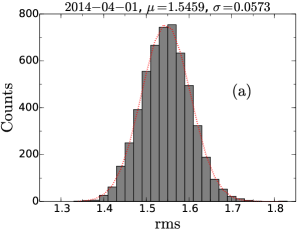
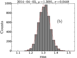
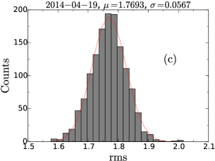
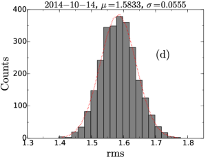
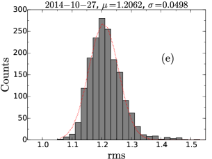
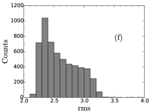
Figure 3: Distributions of the rms of the baseline noise for observations of this study (panels (a) to (e)) and Wen et al. (2016) (panel (f)). The red dotted lines are Gaussian distributions that have been fitted to the rms histograms.

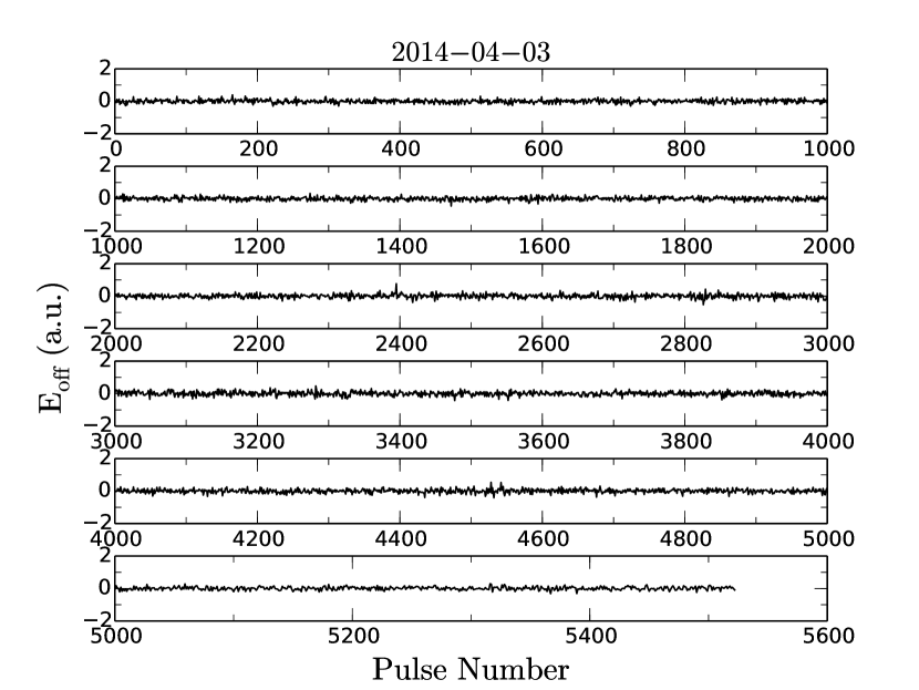
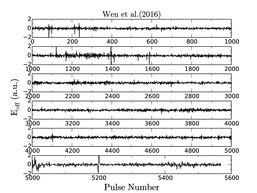
Figure 4: Off-pulse energy variations with time for the 2014-04-03 observation (left) and the observation of Wen et al. (2016) (right).

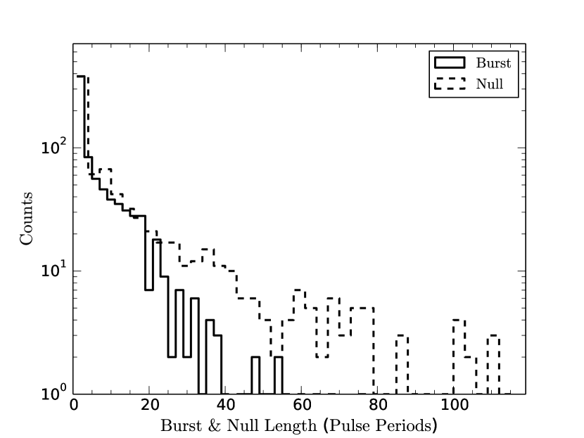
Figure 5: Distributions of the durations of the burst (solid line) and null (dashed line) states.

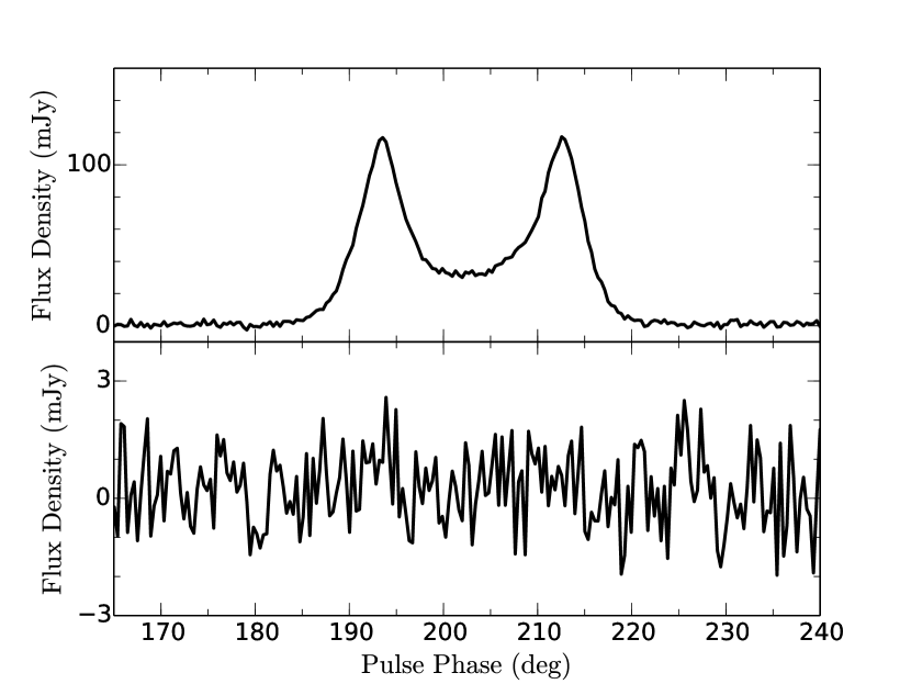
Figure 6: Mean pulse profiles of null (lower) and burst pulses (upper) for the 2014-04-01 observation (see Table 1 for details).

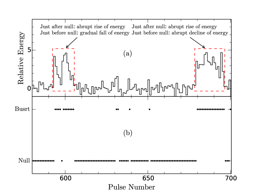
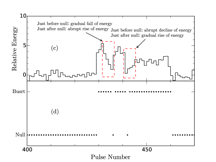
Figure 7: Panels (a) and (c) show on-pulse energy vs. pulse number for two pulse sequences. Panels (b) and (d) show the identified burst or null states for each pulse.

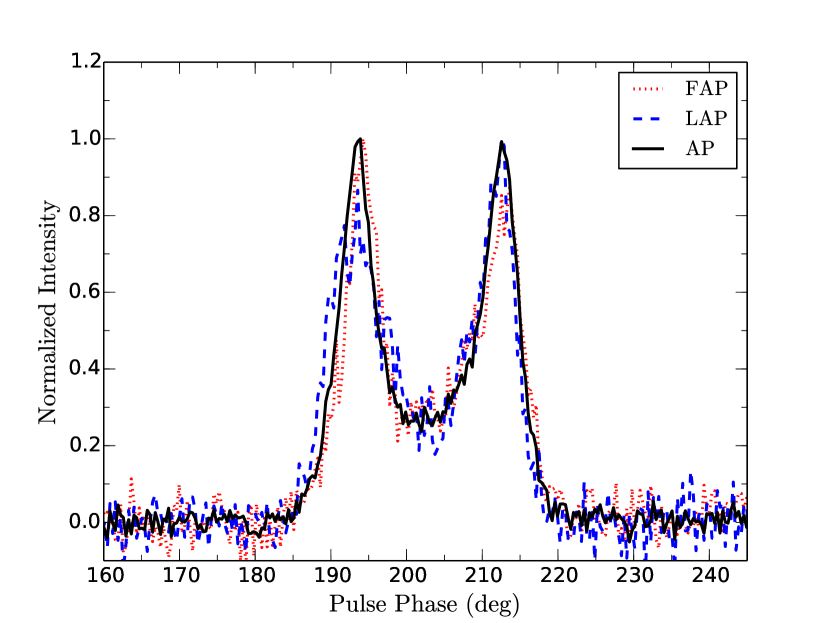
Figure 8: Integrated profiles for the first active pulses (dotted line) and the last active pulses (dashed line) of the burst states. The solid line shows the mean pulse profile of all burst pulses. All profiles are normalized by their respective peak intensities.

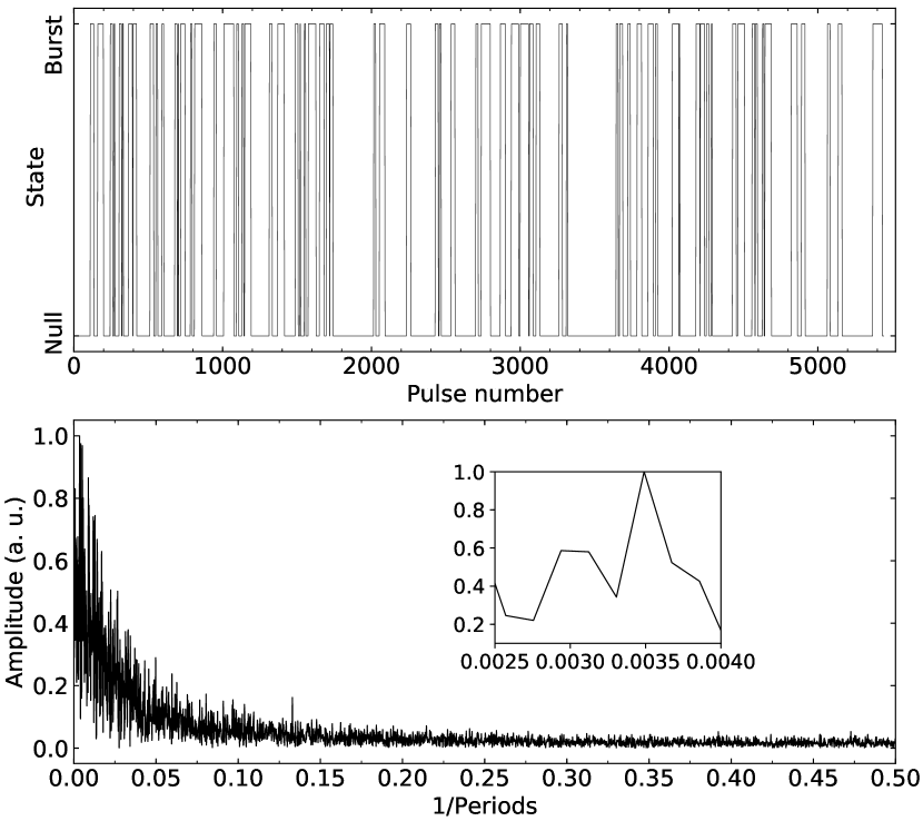
Figure 9: Low-frequency quasi-periodic fluctuations in the pulse energy of PSR J1727$-$2739. The upper panel shows the identified emission states (null or burst) corresponding to each spin period for the 2014-04-03 observation (see Table 1 for details). The lower panel shows the Fourier spectrum of the one-zero sequence (see the text for details) for the same observation. The inset plot exhibits the zoom in on the strongest spectral feature.

The pulse energy variations with time of PSR J1727$-$2739 are presented in Fig. 1 which shows many blocks of consecutive strong pulses separated by frequent nulls. The pulse energy distributions for the on-pulse and off-pulse windows are shown in Fig. 2. We obtained the on-pulse energy for each single pulse by summing the intensities of the pulse phase bins within the on-pulse window of the mean pulse profile. The on-pulse window was defined as the total longitude range over which significant pulsed emission is seen. Similarly, the off-pulse energy was estimated using an off-pulse window of the same length. In Fig. 2, the on-pulse energy histograms show a clear bimodal distribution with two peaks, one at the zero energy and the other at the mean pulse energy. The two distribution modes belong to null and burst states, respectively.

To estimate the baseline noise level of each observation, we first normalized individual pulses with the peak intensity of the mean pulse profile in the corresponding day. Then the rms of the off-pulse region were estimated for all normalized single pulses. The rms distributions for all five observations are given in Fig. 3 (see panels (a) – (e)). The rms distribution of each of our observation can be fitted with a Gaussian function. The best fitted $\mu$ and $\sigma$ are the mean rms and its uncertainty, respectively, which are presented in Table  1. For comparison, using the same method, we estimated the rms distribution for the observation of Wen et al. (2016) which is shown in panel (f) of Fig. 3. Surprisingly, this distribution does not follow a Gaussian form. To explore the possible reason of the deviation from a Gaussian distribution, we compare the temporal variations of the off-pulse energy for observations of this study and Wen et al. (2016), and the results are shown in Fig. 4. We can clearly see that the observation of Wen et al. (2016) shows random and significant fluctuations in off-pulse energy, which is probably due to the presence of strong RFI. We thefore suggest that the deviation from a Gaussian distribution for the rms distribution of Wen et al. (2016) probably arises from the relatively strong RFI. The five distributions of our observations have slightly different mean values of the rms. To reduce the effect of different baseline rms noise levels between different observations, we calculate the NF for every observation separately. Following earlier studies (Ritchings, 1976; Wang et al., 2007; Wen et al., 2016), we estimated the NF of each observation by subtracting a scaled version of the off-pulse histogram from the on-pulse histogram so that the sum of the difference counts in bins with $E<0$ was zero. The NF uncertainty is then given by $\sqrt{n_{\rm p}}/N$, where $n_{\rm p}$ is the number of null pulses and $N$ is the total number of pulses (Wang et al., 2007). The results for the five observations are listed in Table 1. The weighted average of NF of the five observations is $66\%\pm 1.4\%$ which is in good agreement with the previous work (Wen et al., 2016).

Identifying the burst and null states is required for further investigation of the properties of the burst and null pulses. We followed Bhattacharyya et al. (2010) to identify null pulses. First, we calculated the uncertainty of the on-pulse energy $\sigma_{\rm ep}=\sqrt{n_{\rm on}}$ $\sigma_{\rm off}$ for each individual pulse, where $n_{\rm on}$ is the number of on-pulse longitude bins and $\sigma_{\rm off}$ is the rms of the off-pulse region for individual pulses. Then, the pulses with on-pulse energies lower than a threshold of $3\sigma_{\rm ep}$ are classified as null pulses and the others as burst pulses.

The length distributions of identified burst and null are shown in Fig. 5. Both burst and null lengths clearly cluster between two to five pulse periods, which means that the pulsar switches frequently between burst and null states within several spin periods. Backer (1970a) investigated the nulling phenomenon in four pulsars and he divided the nulls into two types according to their duration: Type I nulls have a width between three and ten pulses periods, whereas Type II nulls have a width of only one or two pulses. In this paper, we refer to Type I nulls as long nulls and Type II nulls as short nulls. Both types of nulls are observed in PSR J1727$-$2739.

After the separation of null and burst states, the mean pulse profile obtained from the null and the burst pulses are presented in Fig. 6. In the lower panel, the average profile of null pulses does not exhibit any significant emission component. This implies the absence of any detectable emission during the null state.

The transitional patterns between burst and null states help to understand the triggering and transition mechanism. In PSR B0818$-$41, it was reported that the transitions from bursts to nulls are gradual, while the transitions from nulls to bursts are abrupt (Bhattacharyya et al., 2010). Wen et al. (2016) found an extra transitional pattern in PSR J1727$-$2739, in which the transitions from bursts to nulls can be gradual or abrupt. However, they did not report the transitional pattern of short nulls. Two examples of the zoom-in view of pulse energy variations with time to illustrate the transitional patterns are presented in Fig. 7. All transitional patterns reported by Wen et al. (2016) are shown in the upper part of Fig. 7. In the lower part, two short nulls show totally different transitional patterns. The left short null shows that the transition from a burst to a null is gradual and the transitions from a null to a burst is abrupt, whereas the right short null shows that the transition from a burst to a null is abrupt and the transition from a null to a burst is gradual.

Differences in the shape of the average pulse profiles for the first active pulse (FAP) after a null and the last active pulse (LAP) before a null have been reported in several pulsars (e.g., Deich et al., 1986; Gajjar et al., 2014). We derived the average pulse profiles of the FAP and LAP for PSR J1727$-$2739 and the result is shown in Fig. 8. For the FAP profile, the peak intensities of the leading and trailing components are 1 and 0.87, respectively, and the difference between the two peaks is 0.13. For the LAP profile, the peak intensities of the leading and trailing components are 0.86 and 1, respectively, and the difference between the two peaks is 0.14. For comparison, the rms values of baseline noise are 0.04 and 0.06 for the FAP and LAP proflies, respectively. Our results are in good agreement with those of Wen et al. (2016). The observed profile shape differences between the LAP and FAP imply that the plasma conditions in the magnetosphere may be different at the start and end of burst states.

Basu et al. (2017) reported that the transitions between the burst and null states of PSR J1727$-$2739 show a long periodicity of $206\pm 33P_{1}$. To investigate if the long periodicity exists in our data, we carried out a similar analysis to Gajjar et al. (2017) for the three relatively longer observations (2014-04-01, 2014-04-03 and 2014-10-14). We set burst pulses as ones and null pulses as zeros, then a Fourier transform was performed on this one-zero sequence and the results of the 2014-04-03 observation are given in Fig. 9. Note that, following Gajjar et al. (2017), short bursts and short nulls that last for only one or two periods were ignored in the one-zero sequence. A very clear quasi-periodic feature can be seen at very low frequency in Fig. 9. Results of the three longer observations were averaged and we finally obtained an average periodicity of $243\pm 65P_{1}$. This is consistent with the result of Basu et al. (2017) within the uncertainties.

3.2 Subpulse drifting

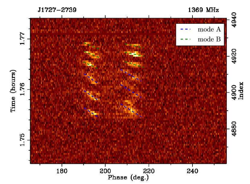
Figure 10: A single-pulse stack showing an example of the rapid switching between different drift modes in the leading and trailing components. The drift bands are indicated by dashed lines.

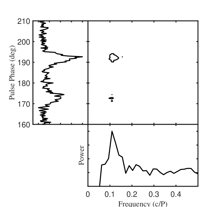
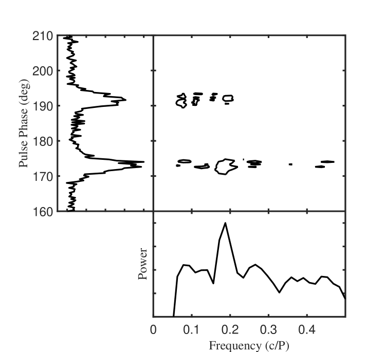
Figure 11: Contour plots for the power spectrum of the flux density as a function of pulse phase for two drift sequences. The upper plot shows a 0.1 c/$P_{1}$ periodicity, while the lower plot shows a 0.2 c/$P_{1}$ periodicity. The left side panels present the power integrated over frequency. The lower side panels give the power integrated over pulse phase. Power at frequencies lower than 0.05 c/$P_{1}$ has been set to zero.

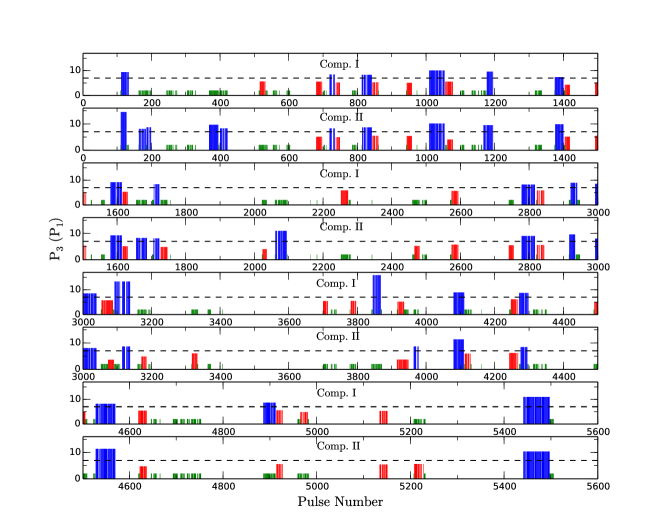
Figure 12: Drift sequences showing observed $P_{3}$ values. Comp. I and Comp. II represent the leading and trailing components, respectively. The modes A and B are plotted with blue and red bars, respectively. Green bars gives burst sequences showing no detection of subpulse drifting. The blank areas correspond to nulls. $P_{3}=7$ is plotted with horizontal dashed-lines, which is the selected threshold for drift mode separation.

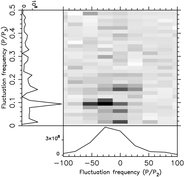
Figure 13: The 2DFS with side panels showing horizontally (left) and vertically (bottom) integrated power for two drift sequences. The left plot shows the mode A of a sequece of 76 pulses with $P_{3}=10.5\pm 0.1~{}P_{1}$ and $P_{2}=14\aas@@fstack{\circ}3\pm 1\aas@@fstack{\circ}3$ in the leading component. The right plot shows the mode B of a sequence of 17 pulses with $P_{3}=5.2\pm 0.1~{}P_{1}$ and $P_{2}=19\aas@@fstack{\circ}6\pm 2\aas@@fstack{\circ}4$ in the trailing component.

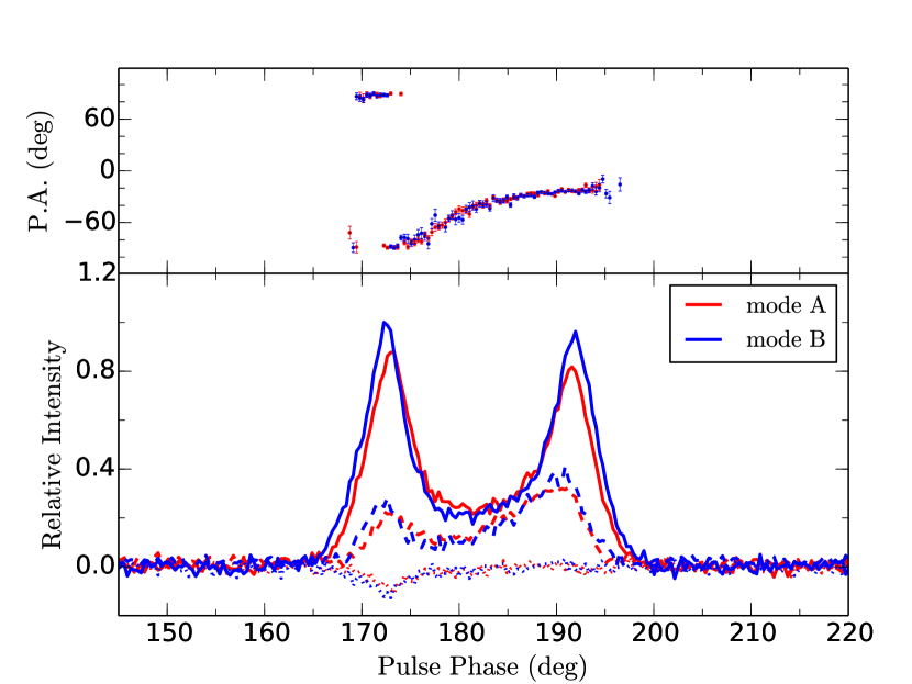
Figure 14: Polarization profiles of different drift modes. For each mode, the lower panel shows the pulse profile for total intensity (solid line), linearly polarized intensity (dashed line), and circularly polarized intensity (dotted line). The upper panel gives the position angles of the linearly polarized emission.

Table 2: Drift parameters for different drift modes. $\rm N_{\rm S}$ stands for number of sequences.

Drift	$P_{\rm 3,l}$	$P_{\rm 2,l}$	$P_{\rm 3,t}$	$P_{\rm 2,t}$	$\Delta\phi_{\rm l}$	$\Delta\phi_{\rm t}$	Number of	Number of	$\rm W_{50}$	$\rm W_{10}$
mode	$(P_{\rm 1})$	$(\degr)$	$(P_{\rm 1})$	$(\degr)$			sequences	pulses	$(\degr)$	$(\degr)$
A	$9.7\pm 0.4$	$16.8\pm 2.8$	$10.0\pm 0.3$	$22.4\pm 3.7$	$1.7\pm 0.1$	$2.2\pm 0.1$	103	2264	$23.8\pm 0.3$	$29.5\pm 0.9$
B	$5.3\pm 0.2$	$16.9\pm 3.0$	$5.1\pm 0.1$	$23.4\pm 4.1$	$3.2\pm 0.1$	$4.6\pm 0.1$	97	1605	$24.5\pm 0.4$	$30.7\pm 0.6$
C	$-$	$-$	$-$	$-$	$-$	$-$	$-$	1083	$24.5\pm 0.4$	$31.2\pm 0.7$

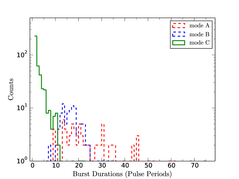
Figure 15: Burst duration distributions of different drift modes.

Based on the leading profile component, Wen et al. (2016) carried out a detailed analysis of the subpulse drifting for PSR J1727$-$2739 at 1518 MHz. They reported that this pulsar shows two distinct drift modes, together with a non-drift mode. The two drift modes were also detected at 610 MHz by Basu et al. (2021). Wen et al. (2016) also noticed the existence of an irregular drifting in the trailing component. However, no further detailed measurements had been performed, probably due to the poor S/N of their data. Fig. 10 shows a single pulse stack which exhibits clear subpulse drifting in both the leading and the trailing components.

In order to identify different drift modes, following earlier studies (Smits et al., 2005; Wen et al., 2016), we used the phase-averaged power spectrum (PAPS) to analyse our data. A candidate drift sequence was first selected visually. Then we computed the PAPS, which is the sum of the amplitudes of the Discrete Fourier Transform (DFT) of each phase bin in a selected pulse-phase window, for this candidate drift sequence. The start and end of the sequence were then adjusted until the peak S/N of PAPS (i.e., the peak value in the PAPS divided by the rms of the rest of the PAPS) was maximized. The reciprocal of the frequency of the PAPS peak was calculated as the drift periodicity $P_{3}$. As is shown in Fig. 10, drifting can be clearly seen in both profile components, we therefore performed the PAPS analysis for both the leading and the trailing components. Fig. 11 gives results of the PAPS analysis of two drift sequences that belong to two different drift modes. The upper half of Fig. 11 shows the PAPS of a sequence of 31 pulses with a peak around 0.1 c/$P_{1}$, which corresponds to $P_{3}\sim$ 10$P_{1}$ for the trailing component. The lower half shows the PAPS of a sequence of 30 pulses with a peak around 0.2 c/$P_{1}$, which corresponds to $P_{3}\sim$ 5$P_{1}$ for the leading component.

Fig. 12 shows the $P_{3}$ values of both components for the 2014-04-01 observation. In agreement with (Wen et al., 2016), the $P_{3}$ values of the leading component can be grouped into two distinct classes, viz., $P_{3}\sim$ 10 $P_{1}$ ( blue in Fig. 12) and $P_{3}\sim$ 5 $P_{1}$ ( red in Fig. 12). The trailing component shows a very similar distribution of $P_{3}$ to the leading component, which means that the trailing component also shows two drift modes with similar periodicities to those of the leading component. This indicates that the drift modes of both components have a common origin. By the PAPS technique, we can divide all burst pulse sequences into different drift modes according to their $P_{3}$ values. Here, we defined pulse sequences with the leading or trailing component showing $P_{3}\sim$10 $P_{1}$ as drift mode A, and those with the leading or trailing component showing $P_{3}\sim$ 5$P_{1}$ as drift mode B. Pulse sequences without any detection of subpulse drifting in either component were classified as drift mode C for convenience. Based on Fig. 12, we tried to find evidence of interactions between nulling and subpulse drifting in PSR J1727$-$2739. We found clues about links between nulling and subpulse drifting. About 67% of the drift sequences of mode A follow behind nulls, while more than 80% of the drift sequences of mode B precede nulls.

After the drift mode separation, we carried out an analysis of fluctuation spectra for each drift sequence to investigate the $P_{2}$ periodicities using the PSRSALSA package. Fig. 13 presents two examples of the resulted two-dimensional fluctuation spectrum (2DFS, Edwards & Stappers (2002)). Table 2 shows a summary of the drift parameters for different modes. Columns (2) and (3) give the values of $P_{3}$ and $P_{2}$, respectively, for the leading component. Columns (4) and (5) show the values of $P_{3}$ and $P_{2}$, respectively, for the trailing component. Columns (6) and (7) present the drift rate $\bigtriangleup\phi$ for the leading and trailing components, respectively. Columns (8) and (9) give the number of sequences and the number of pulses, respectively. The last two columns show the pulse width at 50 per cent of the peak flux density and pulse width at 10 per cent of the peak flux density, respectively. Note that all values of $P_{3}$ and $P_{2}$ in Table 2 were averaged over drift sequences in corresponding drift modes. Although both components have very similar $P_{3}$ in the same drift mode, the $P_{2}$ we measured of the trailing component is larger than that of the leading component by a factor of 1.3. Thus, the drift rate of the trailing component is significantly larger than that of the leading component in the same drift mode. This means that the drift rate changes not only between drift modes but also between profile components. Like PSR B0031$-$07 where $P_{2}$ for three different drift modes are the same (Huguenin et al., 1970; Smits et al., 2005), the $P_{2}$ of PSR J1727$-$2739 measured by us remains unchanged in different drift modes. However, Wen et al. (2016) reported that the measured $P_{2}$ for mode A is larger than that for mode B by a factor of 1.43. In our data, 43% of burst pulses was in the drift mode A and 30% was in the drift mode B. By comparison, Wen et al. (2016) found that the occurrence rate was 49% for mode A and 29% for mode B.

Fig. 14 shows the polarization profiles of different drift modes. In general, there is no significant difference between these polarization profiles. Their PA swings look identical. This implies that different drift modes come from the same region in the magnetosphere. The length distributions of different drift modes are shown in Fig. 15. Our results are consistent with those of Wen et al. (2016). The length of the mode B clearly cluster between 5 to 35 pulse periods, whereas the length of the drift mode A is more evenly distributed.

4 Discussion and conclusions

In this paper, we have conducted a detailed analysis of new single-pulse observations of PSR J1727$-$2739 with the Parkes 64-m radio telescope at 1369 MHz. New results on the properties of nulling and subpulse drifting for this pulsar have been reported.

In agreement with previous work (Wen et al., 2016), we estimate the NF to be $66\%\pm 1.4\%$ for PSR J1727$-$2739 at 1369 MHz. To investigate whether the observed nulls are real nulls or weak modes, we separated all the nulls and burst pulses. We did not find any detectable emission in the average profile of null pulses. This suggests that the observed nulls are true nulls and are not weak modes. The previously reported transitional patterns between bursts and nulls of PSR J1727$-$2739 were also observed in this paper. Furthermore, we observed the transitional patterns between bursts and short nulls that had not been published previously (Fig. 7). We confirm the existence of the long periodicity in the transitions between the burst and null states which was discovered by Basu et al. (2017) and our measured periodicity is $243\pm 65P_{1}$. A study of periodic nulling and periodic amplitude modulations have been carried out in a large number of pulsars by Basu et al. (2020c).

The pattern of arrangement of nulls varies significantly from pulsar to pulsar. Even if two pulsars have the same NF, their null lengths can be very different (Gajjar et al., 2012). Based on a detailed analysis of nulling for 36 pulsars, Basu et al. (2017) concluded that the most dominant nulls lasted for a short duration, less than five periods. Consistent with such results, we found that the burst and null lengths of PSR J1727$-$2739 show similar distributions (Fig. 5) that cluster between two and five pulse periods. However, Wen et al. (2016) presented significantly different distributions of burst and null lengths. In Wen et al. (2016), PSR J1727$-$2739 shows clustering at burst length of around 20 pulse periods while the null length distribution seems to have a favour of around 5$-$35 pule periods. Such differences probably result from the relatively low S/N of the data of Wen et al. (2016). In the case of lower S/N, it becomes difficult to identify true null pulses from burst pulses. Differences in identification of true null and burst pulses can cause large differences in the obtained null length and burst length distributions, specially near the short nulls and short bursts (Gajjar, 2017; Cordes, 2013). Here, we classified pulses with on-pulse energy below the threshold $3\sigma_{\rm ep}$ as null pulses, whereas Wen et al. (2016) used a threshold of $5\sigma_{\rm ep}$. We also tried to use $5\sigma_{\rm ep}$ as the threshold, but the derived average profile of null pulses shows an obvious emission component. We therefore chose $3\sigma_{\rm ep}$, which is more suitable for our data, as the threshold for identification of null and burst pulses.

Consistent with previously published results, we observe two distinct drift modes in PSR J1727$-$2739: mode A (with $P_{3}\sim$ 10$P_{1}$) and mode B (with $P_{3}\sim$ 5$P_{1}$). Compared with Wen et al. (2016), we have some new findings about the drifting behaviour of PSR J1727$-$2739. Apart from the previously known subpulse drifting in the leading component, we found that the trailing component also shows subpulse drifting. In a given drift mode, the drift periodicity $P_{3}$ is constant across all profile components, but the measured $P_{2}$ values are quite different for both components. Contrary to the previous results, we find that the periodicity $P_{2}$ remains unchanged between drift modes A and B for each profile component. Our results show that the drift rate of the trailing component is larger than that of the leading component in either drift mode. The polarization properties and the PA swings are very similar for the two drift modes and this suggests that different drift modes originate from the same emission region. Such polarization behaviour remaining unchanged with the same PA swing in different emission modes has also been reported in PSRs J1822$-$2256 (Basu & Mitra, 2018), B0329+54 (Brinkman et al., 2019), J2006$-$0807 (Basu et al., 2019b) and J2321+6024 (Rahaman et al., 2021).

The subpulse drifting phenomenon is traditionally explained by the carousel model (Ruderman & Sutherland, 1975; van Leeuwen & Timokhin, 2012), in which discrete emission regions rotate around the magnetic axis. When the line of sight passes through the emission region, drifting subpulses can be seen. The carousel model was successful in interpreting subpulse drifting behaviour of many pulsars (Bhattacharyya et al., 2007; Rankin et al., 2013; Rankin & Rosen, 2014; Bilous, 2018). In the original carousel model, the drift rate remains constant, and thus it is difficult to explain the observed multiple drift modes in a pulsar based on the original carousel model. There are several models exploring the mode changing behaviour in pulsars, such as reconfiguration of pulsar magnetosphere (Timokhin, 2010), multiple magnetospheric states incorporating the apparent motion of the visible point (Yuen, 2019), the ion-proton pulsar polar cap model (Jones, 2020) and the partially screened gap (PSG) model (Gil et al., 2003; Szary et al., 2015) in which the perturbations in the magnetic field due to Hall and thermal drift oscillations change the sparking configuration (Geppert et al., 2021). To explain the three distinct drift modes observed in the conal triple pulsar PSR B1918+19 in the carousel framework, Rankin et al. (2013) explored the view that the observed drift bands result from the first-order alias of a faster drift of subbeams equally spaced around the cones. They found that in PSR B1918+19 the three drift modes have a common circulation period of $12P_{1}$ which is also the periodicity of the quasi-periodic nulls. It is possible to extend the Rankin et al. (2013) model for the drift modes of PSR J1727$-$2739 as well, but unlike PSR B1918+19, PSR J1727$-$2739 has a very long null periodicity which is much longer than the periodicity $P_{3}$ of the drift modes.

PSR J2321+6024 is a drifting pulsar showing three distinct drift modes that have different $P_{3}$ values. Rahaman et al. (2021) used the PSG model to explained the change of drift periodicity of PSR J2321+6024, where a changing surface non-dipolar magnetic field structure is required. By simulation analysis, Basu et al. (2020a) showed that the different types of drifting phase behaviour can be explained by the PSG model using some assumptions of spark dynamics in a non-dipolar inner acceleration region (IAR). These studies imply that the PSG model is a very promising model for explaining the change of $P_{3}$ during drift mode changing and drifting phase behaviour. Thus, the PSG model is a very potential model to account for the drifting behaviour of PSR J1727$-$2739.

There is increasing evidence that nulling, mode changing and subpulse drifting are closely linked to each other. The presence of both nulling and subpulse drifting have been seen in a number of pulsars, such as PSRs B0031$-$07 (Vivekanand & Joshi, 1997; Smits et al., 2005; McSweeney et al., 2017), J1822$-$2256 (Basu & Mitra, 2018), B1944+17 (Deich et al., 1986; Kloumann & Rankin, 2010), B2000+40 (Basu et al., 2020b), J2006$-$0807 (Basu et al., 2019b), B2034+19 (Rankin, 2017), J2321+6024 (Wright & Fowler, 1981; Rahaman et al., 2021) and B2303+30 (Redman et al., 2005). Some pulsars show changes in the drift rate after the null states (van Leeuwen et al., 2003; Janssen & van Leeuwen, 2004). Some pulsars exhibit memory of subpulse phases across nulls (Unwin et al., 1978; Gajjar et al., 2017). The interactions between nulling and subpulse drifting suggest that both nulls and subpulse drifting result from intrinsic changes in the pulsar magnetosphere. Based on observations of 23 pulsars, Wang et al. (2007) proposed that both nulling and mode changing result from changes in the magnetospheric current distribution. Studies of nulling, mode changing and subpulse drifting, and their interactions could provide a fundamental clue to the underlying switching mechanism of changes between different magnetospheric states. We found that PSR J1727$-$2739 tends to start mode A sequences after nulls and to start mode B sequences before nulls.

PSR J1727$-$2739 falls in a rare category of pulsars showing nulling along with drift mode changing, which can provide unique opportunity to understand the links between these phenomena. Although we found evidence of interactions between nulling and subpulse drifting in PSR J1727$-$2739, more comprehensive studies based on more sensitive, longer and multifrequency observations for this kind pulsars would certainly provide intriguing details to understand the true nature and origin of these phenomena.

Data Availability

The data underlying this article are available in the Parkes Pulsar Data Archive at https://data.csiro.au, and can be accessed with the source name J1727$-$2739.

References

- Backer (1970a) Backer D. C., 1970a, Nature, 228, 42
- Backer (1970b) Backer D. C., 1970b, Nature, 228, 1297
- Basu & Mitra (2018) Basu R., Mitra D., 2018, MNRAS, 476, 1345
- Basu & Mitra (2019) Basu R., Mitra D., 2019, MNRAS, 487, 4536
- Basu et al. (2016) Basu R., Mitra D., Melikidze G. I., Maciesiak K., Skrzypczak A., Szary A., 2016, ApJ, 833, 29
- Basu et al. (2017) Basu R., Mitra D., Melikidze G. I., 2017, ApJ, 846, 109
- Basu et al. (2019a) Basu R., Mitra D., Melikidze G. I., Skrzypczak A., 2019a, MNRAS, 482, 3757
- Basu et al. (2019b) Basu R., Paul A., Mitra D., 2019b, MNRAS, 486, 5216
- Basu et al. (2020a) Basu R., Mitra D., Melikidze G. I., 2020a, MNRAS, 496, 465
- Basu et al. (2020b) Basu R., Lewandowski W., Kijak J., 2020b, MNRAS, 499, 906
- Basu et al. (2020c) Basu R., Mitra D., Melikidze G. I., 2020c, ApJ, 889, 133
- Basu et al. (2021) Basu R., Mitra D., Melikidze G. I., 2021, ApJ, 917, 48
- Bhattacharyya et al. (2007) Bhattacharyya B., Gupta Y., Gil J., Sendyk M., 2007, MNRAS, 377, L10
- Bhattacharyya et al. (2010) Bhattacharyya B., Gupta Y., Gil J., 2010, MNRAS, 408, 407
- Bilous (2018) Bilous A. V., 2018, A&A, 616, A119
- Brinkman et al. (2019) Brinkman C., Mitra D., Rankin J., 2019, MNRAS, 484, 2725
- Cordes (2013) Cordes J. M., 2013, ApJ, 775, 47
- Deich et al. (1986) Deich W. T. S., Cordes J. M., Hankins T. H., Rankin J. M., 1986, ApJ, 300, 540
- Drake & Craft (1968) Drake F. D., Craft H. D., 1968, Nature, 220, 231
- Edwards & Stappers (2002) Edwards R. T., Stappers B. W., 2002, A&A, 393, 733
- Force & Rankin (2010) Force M. M., Rankin J. M., 2010, MNRAS, 406, 237
- Gajjar (2017) Gajjar V., 2017, arXiv e-prints, p. arXiv:1706.05407
- Gajjar et al. (2012) Gajjar V., Joshi B. C., Kramer M., 2012, MNRAS, 424, 1197
- Gajjar et al. (2014) Gajjar V., Joshi B. C., Wright G., 2014, MNRAS, 439, 221
- Gajjar et al. (2017) Gajjar V., Yuan J. P., Yuen R., Wen Z. G., Liu Z. Y., Wang N., 2017, ApJ, 850, 173
- Geppert et al. (2021) Geppert U., Basu R., Mitra D., Melikidze G. I., Szkudlarek M., 2021, MNRAS, 504, 5741
- Gil et al. (2003) Gil J., Melikidze G. I., Geppert U., 2003, A&A, 407, 315
- Herfindal & Rankin (2007) Herfindal J. L., Rankin J. M., 2007, MNRAS, 380, 430
- Herfindal & Rankin (2009) Herfindal J. L., Rankin J. M., 2009, MNRAS, 393, 1391
- Hobbs et al. (2004) Hobbs G., et al., 2004, MNRAS, 352, 1439
- Hobbs et al. (2011) Hobbs G., et al., 2011, PASA, 28, 202
- Hotan et al. (2004) Hotan A. W., van Straten W., Manchester R. N., 2004, PASA, 21, 302
- Huguenin et al. (1970) Huguenin G. R., Taylor J. H., Troland T. H., 1970, ApJ, 162, 727
- Janssen & van Leeuwen (2004) Janssen G. H., van Leeuwen J., 2004, A&A, 425, 255
- Jones (2020) Jones P. B., 2020, MNRAS, 492, 5987
- Kloumann & Rankin (2010) Kloumann I. M., Rankin J. M., 2010, MNRAS, 408, 40
- Manchester et al. (2005) Manchester R. N., Hobbs G. B., Teoh A., Hobbs M., 2005, AJ, 129, 1993
- Manchester et al. (2013) Manchester R. N., et al., 2013, PASA, 30, e017
- McSweeney et al. (2017) McSweeney S. J., Bhat N. D. R., Tremblay S. E., Deshpande A. A., Ord S. M., 2017, ApJ, 836, 224
- Mitra & Rankin (2017) Mitra D., Rankin J., 2017, MNRAS, 468, 4601
- Rahaman et al. (2021) Rahaman S. k. M., Basu R., Mitra D., Melikidze G. I., 2021, MNRAS, 500, 4139
- Rankin (1986) Rankin J. M., 1986, ApJ, 301, 901
- Rankin (2017) Rankin J. M., 2017, JA&A, 38, 53
- Rankin & Rosen (2014) Rankin J., Rosen R., 2014, MNRAS, 439, 3860
- Rankin & Wright (2008) Rankin J. M., Wright G. A. E., 2008, MNRAS, 385, 1923
- Rankin et al. (2013) Rankin J. M., Wright G. A. E., Brown A. M., 2013, MNRAS, 433, 445
- Redman et al. (2005) Redman S. L., Wright G. A. E., Rankin J. M., 2005, MNRAS, 357, 859
- Ritchings (1976) Ritchings R. T., 1976, MNRAS, 176, 249
- Ruderman & Sutherland (1975) Ruderman M. A., Sutherland P. G., 1975, ApJ, 196, 51
- Smits et al. (2005) Smits J. M., Mitra D., Kuijpers J., 2005, A&A, 440, 683
- Staveley-Smith et al. (1996) Staveley-Smith L., et al., 1996, PASA, 13, 243
- Szary et al. (2015) Szary A., Melikidze G. I., Gil J., 2015, MNRAS, 447, 2295
- Timokhin (2010) Timokhin A. N., 2010, MNRAS, 408, L41
- Unwin et al. (1978) Unwin S. C., Readhead A. C. S., Wilkinson P. N., Ewing M. S., 1978, MNRAS, 182, 711
- van Leeuwen & Timokhin (2012) van Leeuwen J., Timokhin A. N., 2012, ApJ, 752, 155
- van Leeuwen et al. (2003) van Leeuwen A. G. J., Stappers B. W., Ramachandran R., Rankin J. M., 2003, A&A, 399, 223
- van Straten & Bailes (2011) van Straten W., Bailes M., 2011, PASA, 28, 1
- Vivekanand & Joshi (1997) Vivekanand M., Joshi B. C., 1997, ApJ, 477, 431
- Wang et al. (2007) Wang N., Manchester R. N., Johnston S., 2007, MNRAS, 377, 1383
- Wang et al. (2020) Wang P. F., et al., 2020, A&A, 644, A73
- Weltevrede (2016) Weltevrede P., 2016, A&A, 590, A109
- Weltevrede et al. (2006) Weltevrede P., Edwards R. T., Stappers B. W., 2006, A&A, 445, 243
- Weltevrede et al. (2007) Weltevrede P., Stappers B. W., Edwards R. T., 2007, A&A, 469, 607
- Wen et al. (2016) Wen Z. G., Wang N., Yuan J. P., Yan W. M., Manchester R. N., Yuen R., Gajjar V., 2016, A&A, 592, A127
- Wright & Fowler (1981) Wright G. A., Fowler L. A., 1981, A&A, 101, 356
- Yan et al. (2011) Yan W. M., et al., 2011, MNRAS, 414, 2087
- Yan et al. (2019) Yan W. M., Manchester R. N., Wang N., Yuan J. P., Wen Z. G., Lee K. J., 2019, MNRAS, 485, 3241
- Yan et al. (2020) Yan W. M., Manchester R. N., Wang N., Wen Z. G., Yuan J. P., Lee K. J., Chen J. L., 2020, MNRAS, 491, 4634
- Yuen (2019) Yuen R., 2019, MNRAS, 486, 2011