BICEP/Keck and Cosmological Attractors

Abstract

We discuss implications of the latest BICEP/Keck data release for inflationary models, with special emphasis on the cosmological attractors which can describe all presently available inflation-related observational data. These models are compatible with any value of the tensor to scalar ratio $r$, all the way down to $r=0$. Some of the string theory motivated models of this class predict $10^{{-3}}\leq r\leq 10^{{-2}}$. The upper part of this range can be explored by the ongoing BICEP/Keck observations.

1 Introduction

The new data release from BICEP/Keck considerably strengthened bounds on the tensor to scalar ratio $r$ BICEPKeck:2021gln : $r_{0.05}=0.014^{+0.010}_{-0.011}$ ($r_{0.05}<0.036$ at 95% confidence). The main results are illustrated in BICEPKeck:2021gln by a figure describing combined constraints on $n_{s}$ and $r$, which we reproduce here in Fig. 1. These new results have important implications for the development of inflationary cosmology. In particular, the standard version of natural inflation Freese:1990rb , as well as the full class of monomial potentials $V\sim\phi^{n}$, are now strongly disfavored.

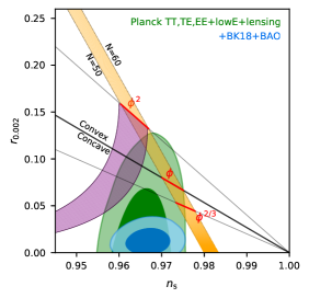
Figure 1: BICEP/Keck results for $n_{s}$ and $r$ BICEPKeck:2021gln . The $1\sigma$ and $2\sigma$ areas are represented by dark blue and light blue colors. The purple region shows natural inflation, and the orange band corresponds to inflation driven by scalar field with canonical kinetic terms and monomial potentials.

Additional information can be obtained for the hilltop models. The simplest models $V=V_{0}(1-\phi^{4}/m^{4})$ represented by the green band in Fig. 8 of the Planck2018 data release Planck:2018jri lead to a universal prediction $n_{s}=1-3/N_{e}$ for all sub-Planckian values of the mass parameter $m\lesssim 1$. This prediction is strongly disfavored by the Planck2018 data for the number of e-foldings $N_{e}\sim 50-60$. These models could provide a good match to the Planck data for $m\gtrsim 10$. However, in that case they predict post-inflationary collapse of the universe, which cannot be avoided without a substantial modification of such models, strongly modifying their predictions Kallosh:2019jnl .

More complicated versions of the hilltop models, such as the new inflation model with the Coleman-Weinberg potential $V\sim 1+{\phi^{4}\over m^{4}}(2\log{\phi^{2}\over m^{2}}-1)$, are marginally compatible with the Planck2018 data Kallosh:2019jnl , though only for $m\gg 1$. Now they are strongly disfavored by the results of the recent BICEP/Keck data release, as we show in Fig. 2.

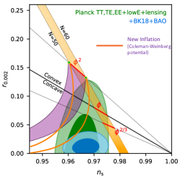
Figure 2: Models of the type of new inflation Linde:1981mu ; Albrecht:1982wi based on the Coleman-Weinberg hilltop potential are marginally compatible with Planck2018 data, but strongly disfavored by the BICEP/Keck data BICEPKeck:2021gln .

However, one can recover these losses by making a relatively simple generalization of the kinetic term of the scalar field. After this generalization, most of the improved models, which we called “cosmological attractors,” become compatible with all presently available inflation-related observational data, almost independently of the choice of the scalar potential prior to the generalization.

2 $\alpha$-attractors

2.1 T-models

We will begin with describing $\alpha$-attractors Kallosh:2013hoa ; Ferrara:2013rsa ; Kallosh:2013yoa ; Galante:2014ifa ; Kallosh:2015zsa ; Kallosh:2019eeu ; Kallosh:2019hzo . The simplest example is given by the theory

$${{\cal L}\over\sqrt{-g}}={R\over 2}-{(\partial_{\mu}\phi)^{2}\over 2\bigl{(}1-{\phi^{2}\over 6\alpha}\bigr{)}^{2}}-V(\phi)\,.$$ (1)

Here $\phi(x)$ is the scalar field, the inflaton. In the limit $\alpha\to\infty$ the kinetic term becomes the standard canonical term $-{(\partial_{\mu}\phi)^{2}\over 2}$. The new kinetic term has a singularity at $|\phi|=\sqrt{6\alpha}$. However, one can get rid of the singularity and recover the canonical normalization by solving the equation ${\partial\phi\over 1-{\phi^{2}\over 6\alpha}}=\partial\varphi$, which yields $\phi=\sqrt{6\alpha}\,\tanh{\varphi\over\sqrt{6\alpha}}$. The full theory, in terms of the canonical variables, becomes a theory with a plateau potential

$${{\cal L}\over\sqrt{-g}}={R\over 2}-{(\partial_{\mu}\varphi)^{2}\over 2}-V\big{(}\sqrt{6\alpha}\,\tanh{\varphi\over\sqrt{6\alpha}}\big{)}\,.$$ (2)

We called such models T-models due to their dependence on the $\tanh{\varphi\over\sqrt{6\alpha}}$. Asymptotic value of the potential at the plateau at large $\varphi>0$ is given by

$$V(\varphi)=V_{0}-2\sqrt{6\alpha}\,V^{\prime}_{0}\ e^{-\sqrt{2\over 3\alpha}\varphi}\ .$$ (3)

Here $V_{0}=V(\phi)|_{\phi=\sqrt{6\alpha}}$ is the height of the plateau potential, and $V^{\prime}_{0}=\partial_{\phi}V|_{\phi=\sqrt{6\alpha}}$. The coefficient $2\sqrt{6\alpha}\,V^{\prime}_{0}$ in front of the exponent can be absorbed into a redefinition (shift) of the field $\varphi$. Therefore all inflationary predictions of this theory in the regime with $e^{-\sqrt{2\over 3\alpha}\varphi}\ll 1$ are determined only by two parameters, $V_{0}$ and $\alpha$, i.e. they do not depend on any other features of the potential $V(\phi)$. That is why they are called attractors.

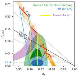
Figure 3: The figure illustrating the main results of the BICEP/Keck BICEPKeck:2021gln superimposed with the predictions of $\alpha$-attractor T-models with the potential $\tanh^{2n}{\varphi\over\sqrt{6\alpha}}$ Kallosh:2013yoa ; Kallosh:2015zsa . Each of these models starts at some $\phi^{2n}$ (at $\alpha\rightarrow\infty$) and is forced to go down with decreasing $\alpha$ Kallosh:2013yoa into the area favored by the BICEP/Keck.

To illustrate advantages of this class of models, we show in Fig. 3 predictions of the models with monomial potentials $\phi^{2n}$ after the modification of the kinetic term shown in (1). At large $\alpha$, predictions of all of these models coincide with the predictions shown in Fig. 1, and these models are ruled out, but at smaller $\alpha$ they all run towards the dark blue area favored by the latest BICEP/Keck data release. Fig. 3 illustrates the main advantage of the cosmological attractors: At large $N_{e}$, their predictions for $A_{s}$, $n_{s}$ and $r$ coincide in the small $\alpha$ limit, nearly independently of the detailed choice of the potential $V(\phi)$:

$$A_{s}={V_{0}\,N_{e}^{2}\over 18\pi^{2}\alpha}\ ,\qquad n_{s}=1-{2\over N_{e}}\ ,\qquad r={12\alpha\over N^{2}_{e}}\ .$$ (4)

These models are compatible with the presently available observational data for sufficiently small $\alpha$.

Importantly, these results depend on the height of the inflationary plateau, which is given by $V_{0}=V(\phi)|_{\phi=\sqrt{6\alpha}}$, but they do not depend on any other details of behavior of the potential $V(\phi)$ in (1). This explains, in particular, stability of the predictions of these models with respect to quantum corrections Kallosh:2016gqp .

The amplitude of inflationary perturbations in these models matches the Planck normalization $A_{s}\approx 2.01\times 10^{{-9}}$ for ${V_{0}\over\alpha}\sim 10^{{-10}}$, $N_{e}=60$, or for ${V_{0}\over\alpha}\sim 1.5\times 10^{{-10}}$, $N_{e}=50$. For the simplest model $V={m^{2}\over 2}\phi^{2}$ one finds

$$V=3m^{2}\alpha\tanh^{2}{\varphi\over\sqrt{6\alpha}}\ .$$ (5)

This simplest model is shown by the prominent vertical yellow band in Fig. 8 of the paper on inflation in the Planck2018 data release Planck:2018jri . In this model, the condition ${V_{0}\over\alpha}\sim 10^{{-10}}$ reads $m\sim 0.6\times 10^{{-5}}$. The small magnitude of this parameter accounts for the small amplitude of perturbations $A_{s}\approx 2.01\times 10^{{-9}}$. No other parameters are required to describe all presently available inflation-related data in this model. If the inflationary gravitational waves are discovered, their amplitude can be accounted for by the choice of the parameter $\alpha$ in (4).

2.2 E-models

The second family of $\alpha$-attractors called E-models is given by

$${{\cal L}\over\sqrt{-g}}={R\over 2}-{3\alpha\over 4}\,{(\partial\rho)^{2}\over\rho^{2}}-V(\rho)\ .$$ (6)

As before, one can go to canonical variables, $\rho=e^{-\sqrt{2\over 3\alpha}\varphi}$, which yields

$${{\cal L}\over\sqrt{-g}}={R\over 2}-{1\over 2}(\partial\varphi)^{2}-V(e^{-\sqrt{2\over 3\alpha}\varphi}).$$ (7)

We consider $V(\rho)$ not singular at $\rho=0$, e.g. $V(\rho)=V_{0}(1-\rho)^{2}$. In canonical variables it gives

$$V=V_{0}\Bigl{(}1-e^{-\sqrt{2\over 3\alpha}\varphi}\Bigr{)}^{2}.$$ (8)

For the particular case $\alpha=1$ this potential coincides with the potential of the Starobinsky model Starobinsky:1980te . In the small $\alpha$ limit the predictions of the E-models coincide with the predictions of the T-models (4).

Fig. 4 shows a combination of predictions of the simplest T-model (5) and the simplest E-model (8). Predictions of both of these models at large $\alpha$ coincide with the predictions of the model $\phi^{2}$, and then go down into the blue area with decreasing $\alpha$. T-model band goes straight, E-model band first slightly bends to the right, to larger values of $n_{s}$, but later reaches the same attractor value as in the T-model. Their predictions are consistent with the Planck/BICEP/Keck bound $r<0.036$ for $\alpha\lesssim 7$. Note that both models can describe any value of $r\ll 1$, all the way down to the ultimate attractor point $r=0$.

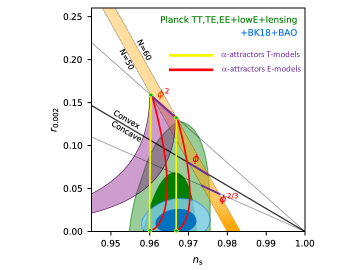
Figure 4: The BICEP/Keck BICEPKeck:2021gln figure superimposed with the predictions of the simplest $\alpha$-attractor T-model with the potential $\tanh^{2}{\varphi\over\sqrt{6\alpha}}$ and E-models (yellow lines for $N_{e}=50,60$) with the potential $\big{(}1-e^{-\sqrt{{2\over 3\alpha}}\varphi}\big{)}^{2}$ (red lines for $N_{e}=50,60$).

3 Other examples of cosmological attractors

3.1 Pole inflation, D-brane inflation

$\alpha$-attractors represent a special version of a more general class of attractors, the so-called pole inflation models Galante:2014ifa . It is obtained by slightly generalizing equation (6):

$${{\cal L}\over\sqrt{-g}}={R\over 2}-{a_{q}\over 2}{(\partial\rho)^{2}\over\rho^{q}}-V(\rho)\ .$$ (9)

Here the pole of order $q$ is at $\rho=0$ and the residue at the pole is $a_{q}$. For $q=2$, $a_{2}={3\alpha\over 2}$, this equation describes E-models of $\alpha$-attractors, but here we consider general values of $q$. For $q\not=2$ one can always rescale $\rho$ to make $a_{q}=1$. Just as in the theory of $\alpha$-attractors, one can make a transformation to the canonical variables $\varphi$ and find that the asymptotic behavior of the potential $V(\varphi)$ during inflation is determined only by $V(0)$ and the first derivative ${dV(\rho)\over d\rho}|_{\rho=0}$ . The value of $n_{s}$ for this family of attractors is given by

$$n_{s}=1-{\beta\over N_{e}}\,,\qquad\beta={q\over q-1}\ .$$ (10)

We will discuss here the models with $q>2$, $\beta<2$, which provide spectral index $n_{s}$ slightly greater than the $\alpha$-attractors result $n_{s}=1-{2\over N_{e}}$ .

For $\alpha$-attractors the plateau of the potential is reached exponentially. For $q>2$ the approach to the plateau is controlled by negative powers of $\varphi$. Some of these models described in Kallosh:2018zsi ; Kallosh:2019eeu ; Kallosh:2019hzo have interpretation in terms of Dp-brane inflation Dvali:1998pa ; Kachru:2003sx . The ${\rm Dp}-{\overline{\rm Dp}}$ brane inflation plateau potentials are

$$V_{Dp-\bar{D}p}\sim{|\varphi|^{k}\over m^{k}+|\varphi|^{k}}=\Big{(}1+{m^{k}\over|\varphi|^{k}}\Big{)}^{-1}\,,\qquad k=7-p={2\over 2-q}\ .$$ (11)

Their attractor formula for the $n_{s}$ is given in (10), whereas the formula for $r$ depends on the parameter $m$ in the potential. For ${\rm D3}-{\overline{\rm D3}}$ inflation for small $m$ one has

$$V=V_{0}\ {\varphi^{4}\over m^{4}+\varphi^{4}}\ ,\qquad n_{s}=1-{5\over 3N_{e}}\ ,\qquad r={4m^{{4\over 3}}\over(3N_{e})^{5\over 3}}\ .$$ (12)

For ${\rm D5}-{\overline{\rm D5}}$ brane inflation one has

$$V=V_{0}\ {\varphi^{2}\over m^{2}+\varphi^{2}}\ ,\qquad n_{s}=1-{3\over 2N_{e}}\ ,\qquad r={\sqrt{2}\,m\over N_{e}^{3\over 2}}\ .$$ (13)

In Fig. (5) we give a combined plot of the predictions of the simplest $\alpha$-attractor models and Dp-brane inflation for $n_{s}$ and $\log_{10}r$, for $N_{e}=50$ and $60$. Kallosh:2019hzo . In the small $m$ limit, the predicted values of $r$ for Dp-brane inflation, and for pole inflation in general, can take extremely small values, all the way down to $r\to 0$.

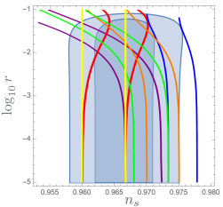
Figure 5: A combined plot of the predictions of the simplest $\alpha$-attractor models and Dp-brane inflation for $N_{e}=50$ and $60$ Kallosh:2019hzo . From left to right, we show predictions of T-models and E-models (yellow and red lines) and of ${\rm Dp}-{\overline{\rm Dp}}$ brane inflation with $p=3,4,5,6$ (purple, green, orange and blue lines) for potentials in eq. (11) with $k=4,3,2,1$. The blue data background corresponds to Planck 2018 results including BAO.

The potentials which appear in the pole inflation scenario may have an alternative interpretation, not related to Dp-branes. For example, a quadratic model $V\sim{\varphi^{2}\over m^{2}+\varphi^{2}}$ was proposed in Dong:2010in as an example of a flattening mechanism for the $\varphi^{2}$ potential due to the inflaton interactions with heavy scalar fields. Similar potentials with flattening may also appear in axion theories in the strong coupling regime DAmico:2017cda .

Independently of their interpretation, the pole inflation models may serve as a powerful tool for parametrization of all observational data since all data for $n_{s}$ and $r$ can be sorted out using vertical $\beta$ stripes with $n_{s}=1-{\beta\over N_{e}}$ Kallosh:2019eeu ; Kallosh:2019hzo . As illustrated by Fig. (5), just a few of such stripes may completely cover all possible values of $n_{s}$ and $r$ compatible with the observational data. This parametrization works especially well in the small $r$ limit, which is the top priority for parametrizing the results of the ongoing and planned search for the inflationary gravitational waves.

3.2 $\xi$-atttractors

Cosmological attractors may also appear in the theories describing non-minimal coupling of scalar fields to gravity Kallosh:2013tua of the form

$${{\cal L}_{\rm J}\over\sqrt{-g}}={1\over 2}\big{(}1+\xi f(\phi)\big{)}R-{1\over 2}(\partial\phi)^{2}-\lambda^{2}f^{2}(\phi)\ .$$ (14)

where $f(\phi)$ is an arbitrary function. In the particular case $V(\phi)=\lambda^{2}f^{2}(\phi)=\lambda^{2}\phi^{4}$, these models coincide with the Higgs inflation model Salopek:1988qh ; Bezrukov:2007ep . Examples of these inflationary models with $V(\phi)\sim\phi^{8},\phi^{6},\phi^{4},\phi^{2},\phi,\phi^{2/3}$ were studied in Kallosh:2013tua and the $n_{s}-r$ plots were given, see Fig. 6. The plots start at $\xi=0$, were there is no non-minimal coupling, and then all models are pushed to smaller $r$ with increasing positive $\xi$. At $\xi\rightarrow\infty$ all models reach the attractor point where $r\approx 3\times 10^{-3}$, as in the Starobinsky model.

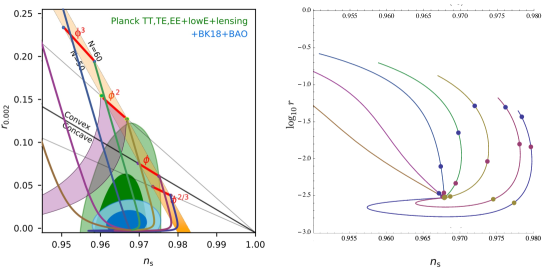
Figure 6: Attractor trajectories for monomial models $V(\phi)\sim\phi^{8},\phi^{6},\phi^{4},\phi^{2},\phi,\phi^{2/3}$, for $N_{e}=60$. In the left panel, the results of Kallosh:2013tua are superimposed with the BICEP/Keck results represented by Fig. 1. The right panel shows the same attractor trajectories, but with the vertical axis corresponding to $\log_{10}r$. This more clearly shows the behavior of these trajectories near the attractor point at large $\xi$ and small $r$. The points on the trajectories shown at the right panel correspond to $\log\xi=-1,0,1$, from top down.

A comparison between Fig. 6 for $\xi$-attractors and the closely related Fig. 3 for the $\alpha$-attractors reveals important similarities and differences. In both cases, the attractor mechanism “saves” the monomial models, making them compatible with the data. But this happens differently for the $\alpha$-attractors and the $\xi$-attractors.

The $\xi$-attractor trajectories in the left panel first go down as straight lines parallel to each other, but then they move to the attractor point almost horizontally, spanning large range of values of $n_{s}$ from $0.96$ to $0.98$ for $r\lesssim 0.01$. This makes such models more robust with respect to future precision data on $n_{s}$.

On the other hand, the values of $r$ for $\xi$-attractors do not go much below $3\times 10^{-3}$, which corresponds to the attractor point for $r$ in the limit $\xi\to\infty$. This is a crucial difference as compared to $\alpha$-attractors, which can describe small $r$ all the way down to $r=0$, corresponding to the attractor point in the limit $\alpha\to 0$.

Thus, if gravitational waves with $r\gtrsim 3\times 10^{-3}$ are not found, it would disfavor $\xi$-attractors, but such result would be quite compatible with $\alpha$-attractors. This particular limitation of $\xi$-attractors disappears if one considers a more general class of models with nonminimal coupling of scalars to gravity

$${{\cal L}_{\rm J}\over\sqrt{-g}}=\frac{1}{2}\Omega(\phi)R-\frac{1}{2}K_{\rm J}(\phi)(\partial\phi)^{2}-V_{\rm J}(\phi)\,.$$ (15)

One can show that for certain relations between $\Omega(\phi)$, $K_{\rm J}(\phi)$ and $V_{\rm J}(\phi)$ this theory in the Einstein frame becomes equivalent to the theory of $\alpha$-attractors Galante:2014ifa . Therefore in this more general context one can describe any small values of $r$.

4 Special cases

So far we presented T- and E-models with a continuous value of $\alpha$, which at small $\alpha$ reach the attractor point with cosmological predictions depending on the number of e-foldings and $\alpha$ as shown in (4). One can implement these models in the minimal ${\cal N}=1$ supergravity, where the parameter $3\alpha$ is given by $3\alpha={1\over 2}|{\cal R}_{K}|$. Here $|{\cal R}_{K}|$ is the curvature of Kähler   geometry Ferrara:2013rsa . In the context of the Poincaré hyperbolic disk geometry, representing an Escher disk, $R^{2}_{\rm Esher}=3\alpha$ defines the size of the disk Kallosh:2015zsa .

The most interesting B-mode targets in this class of cosmological attractor models are the ones with the discrete values of $3\alpha=7,6,5,4,3,2,1$ Ferrara:2016fwe ; Kallosh:2017ced ; Gunaydin:2020ric ; Kallosh:2021vcf . These models of Poincaré disks are inspired by string theory, M-theory and maximal supergravity. They are known in cosmology community, see Fig. 7, which shows the plot of R. Flauger presented in his talk at CMB-S4 collaboration meeting in 2021.

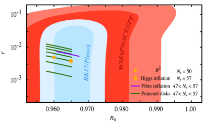
Figure 7: This figure (courtesy of R. Flauger) shows the 7 Poincaré disks of the T-model of $\alpha$-attractors as green lines, as well as Higgs inflation, $R^{2}$ inflation and fibre inflation Cicoli:2008gp . The predictions are for $47<N_{e}<57$.

Fig. 8 shows more detailed plots for the 7 disk predictions for T- and E-models Kallosh:2019hzo . These predictions correspond to the most interesting range $10^{{-2}}\lesssim r\lesssim 10^{{-3}}$.

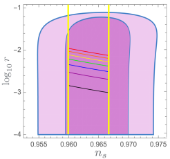
Figure 8: $\alpha$-attractor benchmarks for T-models (left panel) and E-models (right panel) show the discrete values of $3\alpha=7,6,5,4,3,2,1$ from the top going down Kallosh:2019hzo . Dark pink area corresponds to $n_{s}$ and $r$ favored by Planck2018 after taking into account all CMB-related data. The predictions are for $50<N_{e}<60$.

The upper B-mode target with $3\alpha=7$, $r\sim 0.01$ is very close to the range that can be explored by BICEP/Keck, if not now, then within the next five years, when the authors of BICEPKeck:2021gln hope to reach accuracy $\sigma(r)\sim 0.003$. To illustrate what this might entail, we add to Fig. 4 two dashed lines, which show predictions for $3\alpha=7$ for the simplest T-models (yellow dashed line) and E-model (red dashed line) Kallosh:2021vcf . As one can see, these predictions are positioned right at the center of the dark blue ellipse in Fig. 9.

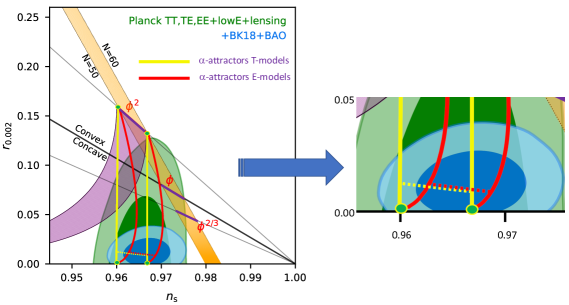
Figure 9: BICEP/Keck results and the predictions for the simplest T-model (yellow dashed line) and E-model (red dashed line) for $3\alpha=7$. These dashed lines go through the center of the dark blue area favored by the combination of the Planck, BICEP and Keck results.

5 Discussion

The new BICEP/Keck constraints on the tensor to scalar ratio $r$ strongly disfavor several popular inflationary models, such as natural inflation, the models with monomial potentials, and the Coleman-Weinberg potentials. However, some of these models have powerful theoretical motivation and can have interesting generalizations. For example, the authors of natural inflation proposed the natural chain inflation scenario Freese:2021noj which may be compatible with the data. The simplest models of axion monodromy scenario Silverstein:2008sg ; McAllister:2014mpa lead to monomial potentials, but allow for various modifications changing the predicted values of $n_{s}$ and $r$, see e.g. Wenren:2014cga ; DAmico:2021vka .

A particularly interesting inflationary model, which fit the Planck/BICEP/Keck data, is the fibre inflation model based on string theory Cicoli:2008gp with the prediction $r\sim 0.007$ indicated by a purple line in Fig. 7. Other examples of inflationary models which can be compatible with the current and future data can be found, in particular, in Enckell:2018uic ; Ellis:2020lnc ; Hazra:2021eqk .

It is most interesting that some models proposed many decades ago and based on entirely different ideas, such as the Starobinsky model Starobinsky:1980te , the Higgs inflation model Salopek:1988qh ; Bezrukov:2007ep , and the GL model Goncharov:1983mw ; Linde:2014hfa , require just a single parameter to successfully account for all presently available data. In this paper we described a broad class of cosmological attractors Kallosh:2013hoa ; Ferrara:2013rsa ; Kallosh:2013yoa ; Galante:2014ifa ; Kallosh:2015zsa ; Kallosh:2019eeu ; Kallosh:2019hzo , which generalized the three models mentioned above.

As discussed in Section 2, $\alpha$-attractors, such as T-models (2) and E-models (7), provide a good fit to the Planck and BICEP/Keck data and have ample flexibility to describe any  value of $r$ below the BICEP/Keck bound $0.036$. A broad class of pole inflation models (9), D-brane models (11), and models describing general non-minimal coupling of scalar fields to gravity (15) also can describe inflation at very small $r$, all the way down to $r=0$.

On the other hand, some string theory inspired versions of $\alpha$-attractors described in Section 4 predict a discrete spectrum of 7 different values of r in the range from $10^{-2}$ to $10^{{-3}}$. The upper one of these predictions is shown in Fig. 9 by the dashed lines going through the center of the dark blue area favored by the combination of the Planck, BICEP and Keck results.

At present, the error bars of the BICEP/Keck estimate $r=0.014\pm 0.01$ are large, $\sigma(r)\sim 0.009$. However, the authors of BICEPKeck:2021gln expect that within the next few years they may improve the accuracy up to $\sigma(r)\sim 0.003$. This suggests that the model describing the first discrete target $r\approx 10^{-2}$ for $\alpha$-attractors with $3\alpha=7$ may be either confirmed or ruled out. It will take much more time and probably a satellite mission to reach $r\approx 10^{-3}$, corresponding to the last Poincaré disk in Figs. 7, 8 with $3\alpha=1$.

Addendum: After this paper was submitted, a new set of constraints on $r$ and $n_{s}$ was given in Tristram:2021tvh after a somewhat different analysis of Planck data. The main results of Tristram:2021tvh are very similar to those reported in BICEPKeck:2021gln . According to Tristram:2021tvh , the 2$\sigma$ upper bound on $r$ changes from $r<0.036$ BICEPKeck:2021gln to $r<0.032$. The 1$\sigma$ bound on $n_{s}$ presented in Tristram:2021tvh is shifted to smaller values of $n_{s}$ by $\Delta n_{s}\sim-0.003$. This does not affect conclusions of our paper. If anything, the new constraints given in Tristram:2021tvh make the match between the observations and the predictions of cosmological attractors even better. One can see it by comparing Fig. 9 with Fig. 10, which shows the results of Tristram:2021tvh and the predictions of the simplest T- and E-models of $\alpha$-attractors.

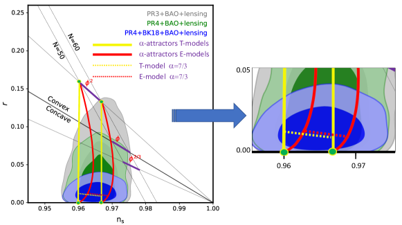
Figure 10: Results of Tristram:2021tvh and the predictions for the simplest T-model (yellow dashed line) and E-model (red dashed line) for $3\alpha=7$. These dashed lines go through the center of the dark blue area favored by the combination of the Planck, BICEP and Keck results according to Tristram:2021tvh .

References

- (1) BICEP/Keck collaboration, Improved Constraints on Primordial Gravitational Waves using Planck, WMAP, and BICEP/Keck Observations through the 2018 Observing Season, Phys. Rev. Lett. 127 (2021) 151301 [2110.00483].
- (2) K. Freese, J.A. Frieman and A.V. Olinto, Natural inflation with pseudo - Nambu-Goldstone bosons, Phys. Rev. Lett. 65 (1990) 3233.
- (3) Planck collaboration, Planck 2018 results. X. Constraints on inflation, Astron. Astrophys. 641 (2020) A10 [1807.06211].
- (4) R. Kallosh and A. Linde, On hilltop and brane inflation after Planck, JCAP 09 (2019) 030 [1906.02156].
- (5) A.D. Linde, A New Inflationary Universe Scenario: A Possible Solution of the Horizon, Flatness, Homogeneity, Isotropy and Primordial Monopole Problems, Phys. Lett. B108 (1982) 389.
- (6) A. Albrecht and P.J. Steinhardt, Cosmology for Grand Unified Theories with Radiatively Induced Symmetry Breaking, Phys. Rev. Lett. 48 (1982) 1220.
- (7) R. Kallosh and A. Linde, Universality Class in Conformal Inflation, JCAP 1307 (2013) 002 [1306.5220].
- (8) S. Ferrara, R. Kallosh, A. Linde and M. Porrati, Minimal Supergravity Models of Inflation, Phys. Rev. D88 (2013) 085038 [1307.7696].
- (9) R. Kallosh, A. Linde and D. Roest, Superconformal Inflationary -Attractors, JHEP 11 (2013) 198 [1311.0472].
- (10) M. Galante, R. Kallosh, A. Linde and D. Roest, Unity of Cosmological Inflation Attractors, Phys. Rev. Lett. 114 (2015) 141302 [1412.3797].
- (11) R. Kallosh and A. Linde, Escher in the Sky, Comptes Rendus Physique 16 (2015) 914 [1503.06785].
- (12) R. Kallosh and A. Linde, B-mode Targets, Phys. Lett. B 798 (2019) 134970 [1906.04729].
- (13) R. Kallosh and A. Linde, CMB Targets after PlanckCMB targets after the latest data release, Phys. Rev. D100 (2019) 123523 [1909.04687].
- (14) R. Kallosh and A. Linde, Cosmological Attractors and Asymptotic Freedom of the Inflaton Field, JCAP 1606 (2016) 047 [1604.00444].
- (15) A.A. Starobinsky, A New Type of Isotropic Cosmological Models Without Singularity, Phys. Lett. 91B (1980) 99.
- (16) R. Kallosh, A. Linde and Y. Yamada, Planck 2018 and Brane Inflation Revisited, JHEP 01 (2019) 008 [1811.01023].
- (17) G.R. Dvali and S.H.H. Tye, Brane inflation, Phys. Lett. B 450 (1999) 72 [hep-ph/9812483].
- (18) S. Kachru, R. Kallosh, A.D. Linde, J.M. Maldacena, L.P. McAllister and S.P. Trivedi, Towards inflation in string theory, JCAP 0310 (2003) 013 [hep-th/0308055].
- (19) X. Dong, B. Horn, E. Silverstein and A. Westphal, Simple exercises to flatten your potential, Phys. Rev. D84 (2011) 026011 [1011.4521].
- (20) G. D’Amico, N. Kaloper and A. Lawrence, Monodromy Inflation in the Strong Coupling Regime of the Effective Field Theory, Phys. Rev. Lett. 121 (2018) 091301 [1709.07014].
- (21) R. Kallosh, A. Linde and D. Roest, Universal Attractor for Inflation at Strong Coupling, Phys. Rev. Lett. 112 (2014) 011303 [1310.3950].
- (22) D.S. Salopek, J.R. Bond and J.M. Bardeen, Designing Density Fluctuation Spectra in Inflation, Phys. Rev. D40 (1989) 1753.
- (23) F.L. Bezrukov and M. Shaposhnikov, The Standard Model Higgs boson as the inflaton, Phys. Lett. B659 (2008) 703 [0710.3755].
- (24) S. Ferrara and R. Kallosh, Seven-disk manifold, -attractors, and modes, Phys. Rev. D94 (2016) 126015 [1610.04163].
- (25) R. Kallosh, A. Linde, T. Wrase and Y. Yamada, Maximal Supersymmetry and B-Mode Targets, JHEP 04 (2017) 144 [1704.04829].
- (26) M. Gunaydin, R. Kallosh, A. Linde and Y. Yamada, M-theory Cosmology, Octonions, Error Correcting Codes, JHEP 01 (2021) 160 [2008.01494].
- (27) R. Kallosh, A. Linde, T. Wrase and Y. Yamada, IIB String Theory and Sequestered Inflation, 2108.08492.
- (28) M. Cicoli, C.P. Burgess and F. Quevedo, Fibre Inflation: Observable Gravity Waves from IIB String Compactifications, JCAP 0903 (2009) 013 [0808.0691].
- (29) K. Freese, A. Litsa and M.W. Winkler, Natural Chain Inflation, 2109.11556.
- (30) E. Silverstein and A. Westphal, Monodromy in the CMB: Gravity Waves and String Inflation, Phys. Rev. D78 (2008) 106003 [0803.3085].
- (31) L. McAllister, E. Silverstein, A. Westphal and T. Wrase, The Powers of Monodromy, JHEP 09 (2014) 123 [1405.3652].
- (32) D. Wenren, Tilt and Tensor-to-Scalar Ratio in Multifield Monodromy Inflation, 1405.1411.
- (33) G. D’Amico, N. Kaloper and A. Westphal, Double Monodromy Inflation: A Gravity Waves Factory for CMB-S4, LiteBIRD and LISA, 2101.05861.
- (34) V.-M. Enckell, K. Enqvist, S. Rasanen and L.-P. Wahlman, Higgs- inflation - full slow-roll study at tree-level, JCAP 01 (2020) 041 [1812.08754].
- (35) J. Ellis, M.A.G. Garcia, N. Nagata, N.D. V., K.A. Olive and S. Verner, Building models of inflation in no-scale supergravity, Int. J. Mod. Phys. D 29 (2020) 2030011 [2009.01709].
- (36) D.K. Hazra, D. Paoletti, I. Debono, A. Shafieloo, G.F. Smoot and A.A. Starobinsky, Inflation Story: slow-roll and beyond, 2107.09460.
- (37) A.B. Goncharov and A.D. Linde, Chaotic Inflation in Supergravity, Phys. Lett. B139 (1984) 27.
- (38) A. Linde, Does the first chaotic inflation model in supergravity provide the best fit to the Planck data?, JCAP 1502 (2015) 030 [1412.7111].
- (39) M. Tristram et al., Improved limits on the tensor-to-scalar ratio using BICEP and Planck, 2112.07961.