SEA: Graph Shell Attention in Graph Neural Networks

Abstract

A common issue in Graph Neural Networks (GNNs) is known as over-smoothing. By increasing the number of iterations within the message-passing of GNNs, the nodes’ representations of the input graph align with each other and become indiscernible. Recently, it has been shown that increasing a model’s complexity by integrating an attention mechanism yields more expressive architectures. This is majorly contributed to steering the nodes’ representations only towards nodes that are more informative than others. Transformer models in combination with GNNs result in architectures including Graph Transformer Layers (GTL), where layers are entirely based on the attention operation. However, the calculation of a node’s representation is still restricted to the computational working flow of a GNN. In our work, we relax the GNN architecture by means of implementing a routing heuristic. Specifically, the nodes’ representations are routed to dedicated experts. Each expert calculates the representations according to their respective GNN workflow. The definitions of distinguishable GNNs result from $k$-localized views starting from the central node. We call this procedure Graph Shell Attention (SEA), where experts process different subgraphs in a transformer-motivated fashion. Intuitively, by increasing the number of experts, the models gain in expressiveness such that a node’s representation is solely based on nodes that are located within the receptive field of an expert. We evaluate our architecture on various benchmark datasets showing competitive results compared to state-of-the-art models.

Introduction

The modeling flow of Graph Neural Networks (GNNs) has been proven to be a convenient tool in a variety of real-world applications building on top of graph data (Wu et al. 2021). These range from predictions in social networks over property predictions in molecular graph structures to content recommendations in online platforms. From a machine learning perspective, we can categorize them into various theoretical problems that are known as node classification, graph classification/regression - encompassing binary decisions or modeling a continuous-valued function -, and relation prediction. In our work, we propose a novel framework and show its applicability on graph-level classification and regression, as well as on node-level classification tasks.

The high-level intuition behind GNNs is that by increasing the number of iterations $k=1,\ldots,K$, a node’s representation processes, contains, and therefore relies more and more on its $k$-hop neighborhood. However, a well-known issue with the vanilla GNN architecture refers to a problem called over-smoothing (Hoory, Linial, and Wigderson 2006; Xu et al. 2018a). Suppose we are given a GNN-motivated model, the information flow between two nodes $u,v\in\mathcal{V}$, where $\mathcal{V}$ denotes a set of nodes, is proportional to the reachability of node $v$ on a $k$-step random walk starting from $u$. Hence, by increasing the layers within the GNN architecture, the information flow of every node approaches the stationary distribution of random walks over the graph. As a consequence, the localized information flow is getting lost. On graph data that follow strong connectivity, it takes $k=O(log|\mathcal{V}|)$ steps for a random walk starting from an arbitrary node to converge to an (almost) uniform distribution. Consequently, increasing the number of iterations within the GNN message-passing results in representations for all the nodes in the input graph that align and become indiscernible.

One strategy for increasing a GNN’s expressiveness is by adding an attention mechanism into the architecture. Recently, it has been shown how the Transformer model (Vaswani et al. 2017) can be applied on graph data (Dwivedi and Bresson 2021) yielding competitive results to state-of-the-art models. Generally, multi-headed attention shows vying results whenever we have prior knowledge to indicate that some neighbors might be more informative than others.

Our framework further improves the representational capacity by adding an expert motivated heuristic into the GNN architecture. More specifically, to compute a node’s representation, a routing module first decides upon an expert that is responsible for a node’s computation. The experts differ in how their $k$-hop localized neighborhood is processed and capture various depths of GNNs. We refer to the different substructures that individual experts process by Graph Shells. As each expert attends to a specific subgraph of the input graph, we introduce the concept of Graph Shell Attention (SEA). Hence, whereas a vanilla GNN lacks in over-smoothing the representations for all nodes, we introduce additional degrees of freedom in our architecture to simultaneously capture short- and long-term dependencies being processed by respective experts.

In summary, our contributions are as follows:

• Integration of expert-routing mechanism into Transformer motivated models applied on graph data;

• Novel Graph Shell Attention (SEA) models relaxing the vanilla GNN definition;

Related Work

In recent years, the AI community proposed various forms of (self-)attention in numerous domains. Attention itself refers to a mechanism in neural networks where a model learns to make predictions by selectively attending to a given set of data. The success of these models dates back to Vaswani et al. (Vaswani et al. 2017) by introducing the Transformer model. It relies on scaled dot-product attention, i.e., given a query matrix $Q$, a key matrix $K$, and a value matrix $V$, the output is a weighted sum of the value vectors, where the dot-product of the query with corresponding keys determines the weight that is assigned to each value.

Transformer architectures have also been successfully applied to graph data. A thorough work by Dwivedi et al. (Dwivedi and Bresson 2021) evaluates transformer-based GNNs. They conclude that the attention mechanism in Transformers applied on graph data should only aggregate the information from the local neighborhood, ensuring graph sparsity. As in Natural Language Processing (NLP), where a positional encoding is applied, they propose to use Laplacian eigenvectors as the positional encodings for further improvements. In their results, they outperform baseline GNNs on the graph representation task. A similar work (Kreuzer et al. 2021) proposes a full Laplacian spectrum to learn the position of each node within a graph. Yun et al. (Yun et al. 2019) proposed Graph Transformer Networks (GTN) that is capable of learning on heterogeneous graphs. The target is to transform a given heterogeneous input graph into a meta-path-based graph and apply a convolution operation afterward. Hence, the focus of their attention framework is on interpreting generated meta-paths. Another transformer-based architecture that has been introduced by Hu et al. (Hu et al. 2020b) is Heterogeneous Graph Transformer (HGT). Notably, their architecture can capture graph dynamics w.r.t the information flow in heterogeneous graphs. Specifically, they take the relative temporal positional encoding into account based on differences of temporal information given for the central node and the message-passing nodes. By including the temporal information, Zhou et al. (Zhou et al. 2020) built a transformer-based generative model for generating temporal graphs by directly learning from the dynamic information in networks. The work of Ngyuen et al. (Nguyen, Nguyen, and Phung 2019) proposes another idea for positional encoding. The authors of this work introduced a graph transformer for arbitrary homogeneous graphs with a coordinate embedding-based positional encoding scheme.

In (Ying et al. 2021), the authors introduced a transformer motivated architecture where various encodings are aggregated to compute the hidden representations. They propose graph structural encodings subsuming a spatial encoding, an edge encoding, and a centrality encoding.

Furthermore, a work exploring the effectiveness of large-scale pre-trained GNN models is proposed by the GROVER model (Rong et al. 2020). The authors include an additional GNN applied in the attention sublayer to produce vectors for $Q$, $K$, and $V$. Moreover, they apply single long-range residual connections and two branches of feedforward networks to produce node and edge representations separately. In a self-supervised fashion, they first pre-train their model on $10$ million unlabeled molecules before using the resulting node representations in downstream tasks.

Typically, all the models are built in a way such that the same parameters are used for all inputs. To gain more expressiveness, the motivation of the mixture of experts (MoE) heuristic (Shazeer et al. 2017) is to apply different parameters w.r.t to the input data. Recently, Google proposed Switch Transformer (Fedus, Zoph, and Shazeer 2021), enabling training above a trillion parameter networks but keeping the computational cost in the inference step constant. In our work, we will show how we can apply MoE motivated heuristics in the scope of GNN models.

Preliminaries

In this section, we provide definitions and recap on the general message-passing paradigm combined with Graph Transformer Layers (GTLs) (Dwivedi and Bresson 2021).

Notation

Let $\mathcal{G}=(\mathcal{V},\mathcal{E})$ be an undirected graph where $\mathcal{V}$ denotes a set of nodes and $\mathcal{E}$ denotes a set of edges connecting nodes. We define $\mathcal{N}_{k}(u)$ to be the $k$-hop neighborhood of a node $u\in\mathcal{V}$, i.e., $N_{k}(u)=\{v\in\mathcal{V}:d_{\mathcal{G}}(u,v)\leq k\}$, where $d_{G}(u,v)$ denotes the hop-distance between $u$ and $v$ on $\mathcal{G}$. For $N_{1}(u)$ we will simply write $N(u)$ and omit the index $k$. The induced subgraph by including the $k$-hop neighbors starting from node $u$ is denoted by $\mathcal{G}_{u}^{k}$. Moreover, in the following we will use a real-valued representation vector $h_{u}\in\mathbb{R}^{d}$ for a node $u$, where $d$ denotes the embedding dimensionality.

Graph Neural Networks

Given a graph $\mathcal{G}=(\mathcal{V},\mathcal{E})$ with node attributes $X_{\mathcal{V}}=\{X_{u}|u\in\mathcal{V}\}$ and edge attributes $X_{\mathcal{E}}=\{X_{uv}|(u,v)\in\mathcal{E}\}$, a GNN aims to learn an embedding vector $h_{u}$ for each node $u\in\mathcal{V}$, and a vector $h_{\mathcal{G}}$ for the entire graph $\mathcal{G}$. For an $L$-layer GNN, a neighborhood aggregation scheme is performed to capture the $L$-hop information surrounding each node. The $l$-th layer of a GNN is formalized as follows:

$$h_{u}^{l+1} =\textsc{update}^{l}(h_{u}^{l},m_{N(u)}^{l})$$ (1)

$$m_{N(u)}^{l} =\textsc{aggregate}^{l}(\{(h_{v}^{l}):v\in N(u)\}),$$ (2)

where $N(u)$ is the $1$-hop neighborhood set of $u$, $h_{u}^{(l)}$ denotes the representation of node $u$ at the $l$-th layer, and $h_{u}^{(0)}$ is initialized as the node attribute $X_{u}$. Since $h_{u}$ summarizes the information of central node $u$, it is also referred as patch embedding in the literature. A graph’s embedding $h_{\mathcal{G}}$ is derived by a permutation-invariant readout function:

$$h_{\mathcal{G}}=\textsc{readout}(\{h_{u}|u\in\mathcal{V}\})$$ (3)

A common heuristic for the readout function is to choose a function $\textsc{readout}(\cdot)\in\{mean(\cdot),sum(\cdot),max(\cdot)\}$.

Transformer

The vanilla Transformer architecture as proposed by Vaswani et al. (Vaswani et al. 2017) was originally introduced in the scope of Natural Language Processing (NLP) and consists of a composition of Transformer layers. Each Transformer layer has two parts: a self-attention module and a position-wise feedforward network (FFN). Let $H=[h_{1}^{T},\ldots,h_{n}^{T}]^{T}\in\mathbb{R}^{n\times d}$ denote the input of the self-attention module where $d$ is the hidden dimension and $h_{i}\in\mathbb{R}^{1\times d}$ is the hidden representation at position $i$ of an input sequence. The input $H$ is projected by three matrices $W_{Q}\in\mathbb{R}^{d\times d_{Q}}$, $W_{K}\in\mathbb{R}^{d\times d_{K}}$, and $W_{V}\in\mathbb{R}^{d\times d_{V}}$ to get the corresponding representation $Q,K,V$. The self-attention is calculated as:

$$\begin{split}Q=HW_{Q}\qquad K=HW_{K}\qquad V=HW_{V},\\ A=\frac{QK^{T}}{\sqrt{d_{k}}},\quad Attn(H)=\operatorname{softmax}(A)V\end{split}$$ (4)

Notably, in NLP as well as in computer vision tasks, the usage of transformer models were boosters behind a large number of state-of-the-art systems. Recently, the Transformer architecture has also been modified to be applicable to graph data (Dwivedi and Bresson 2021), which we will briefly recap in the next section.

Graph Transformer Layer

Figure 1: Vanilla Graph Transformer Layer with edge features (Dwivedi and Bresson 2021); $\lambda$ denotes the Laplacian eigenvectors for positional encodings

Generally, in NLP, the words in an input sequence can be represented as a fully connected graph that includes all connections between the input words. However, such an architecture does not leverage graph connectivity. Therefore, it can perform poorly whenever the graph topology is important and has not been encoded in the input data in any other way. These thoughts lead to the work (Dwivedi and Bresson 2021), where a general Graph Transformer Layer (GTL) has been introduced.

For the sake of completeness, we will recap on the most important equations. A layer update for layer $l$ within a GTL including edge features is defined as:

$$\hat{h}_{u}^{l+1} =O_{h}^{l}\bigparallel_{k=1}^{H}(\sum_{v\in\mathcal{N}_{u}}w_{uv}^{k,l}V^{k,l}h_{v}^{l}),$$ (5)

$$\hat{e}_{uv}^{l+1} =O_{e}^{l}\bigparallel_{k=1}^{H}(\hat{w}_{uv}^{k,l}),\text{where},$$ (6)

$$w_{uv}^{k,l} =\operatorname{softmax}_{v}(\hat{w}_{uv}^{k,l}),$$ (7)

$$\hat{w}_{uv}^{k,l} =(\frac{Q^{k,l}h_{u}^{l}\cdot K^{k,l}h_{v}^{l}}{\sqrt{d_{k}}})\cdot E^{k,l}e_{uv}^{l},$$ (8)

where $Q^{k,l},K^{k,l},V^{k,l},E^{k,l}\in\mathbb{R}^{d_{k}\times d}$, and $O_{h}^{l},O_{e}^{l}\in\mathbb{R}^{d\times d}$. The operator $\bigparallel$ denotes the concatenation of attention heads $k=1,\ldots,H$. Subsequently, the outputs $\hat{h}_{u}^{l+1}$ and $\hat{e}_{uv}^{l+1}$ are passed to feedforward networks and succeeded by residual connections and normalization layers as in the vanilla Transformer architecture (Vaswani et al. 2017). The full architecture of GTLs is illustrated in figure 1.

Positional Encoding. Using the Laplacian eigenvectors as the positional encoding for nodes within a graph is a common heuristic (Dwivedi and Bresson 2021). From spectral analysis, the eigenvectors are computed by the factorization of the Laplacian matrix:

$$\Delta=I-D^{-1/2}AD^{-1/2}=U^{T}\Lambda U,$$ (9)

where $A$ denotes the $n\times n$ adjacency matrix, $D$ denotes the degree matrix. The decomposition yields $\Lambda,U$ corresponding to the eigenvalues and eigenvectors. For the positional encoding, we use the $k$ smallest eigenvectors of a node. In our models, we also apply the Laplacian Positional Encoding (LPE).

Methodology

In this section, we introduce our Graph Shell Attention (SEA) architecture for graph data. SEA builds on top of the message-passing paradigm of Graph Neural Networks (GNNs) and integrates an expert heuristic.

Over-smoothing in GNNs is a well-known issue (Xu et al. 2018a) and exacerbates the problem when we build deeper GNN models which generate similar representations for all nodes in the graph. Applying the same number of iterations for each node inhibits the expressiveness of short- and long-term dependencies simultaneously. Therefore, our architecture loosens up the strict workflow that is applied for each node equally. We gain expressiveness by routing each node representation towards dedicated experts, which only process nodes in their $k$-localized receptive field.

Graph Shells

In our approach, we exploit the graph transformer architecture, including Graph Transformer Layers (GTLs) (Dwivedi and Bresson 2021) and extend it by a set of experts. A routing layer decides upon which expert is most relevant for the computation of a node’s representation. Intuitively, the expert’s computation for a node representation differs in how $k$-hop neighbors are stored and processed within GTLs.

Generally, starting from a central node, Graph Shells refer to subgraphs that include only nodes that have at maximum a $k$-hop distance ($k$-neighborhood). More formally, the $i$-th expert comprises the information given in the $i$-th neighborhood $N_{i}(u)=\{v\in\mathcal{V}:d_{G}(u,v)\leq i)\}$, where $u\in\mathcal{V}$ denotes the central node. We refer to the subgraph $\mathcal{G}_{u}^{i}$ as the expert’s receptive field. Notably, increasing the number of iterations within GNNs correlate with the number of experts being used.

In the following, we introduce three variants on how experts process graph shells.

SEA-gnn

For the definition of the first graph shell model, we exploit the GNN architecture. Hence, the shells described by each expert are given by construction. From the formal definition expressed in eqs. 1 and 2, the information for the $l$-th expert is defined by the $l$-th iteration of the GNN. For $N$ experts, we set the maximal number of hops to be $L=N$. Figure 2(a) illustrates this graph shell model. From left to right, the information of nodes being reachable by more hops is processed. Experts storing information after few hops refer to short-term dependencies, whereas experts processing more hops yields information of long-term dependencies.

SEA-aggregated

For the computation of the hidden representation $h_{u}^{l+1}$ for node $u$ on layer $l+1$, the second model employs an aggregated value from the previous iteration. According to the message-passing paradigm of a vanilla GNN, the aggregation function of eq. 2 considers the $1$-hop neighbors $N_{1}(u)$. For SEA-aggregated, we send the aggregated value $m_{N_{1}}(u)^{l}$ to all its $1$-hop neighbors. For a node $v\in N_{1}(u)$, the values received by $v$ are processed according to another aggregation function which can be chosen among $\textsc{Aggregate}_{\mu}\in\{mean(\cdot),sum(\cdot),max(\cdot)\}$. Formally:

$$h_{u}^{l+1}=\textsc{Aggregate}_{\mu}^{l}((m_{N(v)}^{l}):v\in N(u)\})$$ (10)

Figure 2(b) illustrates this graph shell model. In the first iteration, there are no proceeding layers. Hence, the first expert processes in the same way as the first model. The representations for the second expert are computed by taking the aggregated values of the first shell into account. Sending values to neighboring nodes is illustrated by a full-colored shell.

SEA-k-hop

For this model we relax the aggregate function defined in eq. 2. Given a graph $\mathcal{G}$, we also consider $k$-hop linkages in the graph connecting a node $u$ with all entities having a maximum distance of $d_{\mathcal{G}}(u,v)=k$. The relaxations of eqs. 1 and 2 can then be written as:

$$h_{u}^{l+1} =\textsc{update}^{l}(h_{u}^{l},m_{N_{k}(u)}^{l})$$ (11)

$$m_{N_{k}(u)}^{l} =\textsc{aggregate}^{l}(\{(h_{v}^{l}):v\in N_{k}(u)\}),,$$ (12)

where $N_{k}(u)$ denotes the $k$-hop neighborhood set. This approach allows for processing each $N_{1}(u),\ldots,N_{k}(u)$ with their own submodules, i.e., for each $k$-hop neighbors we use respective feedforward networks to compute $Q,K,V$ in GTLs. Notably, this definition can be interpreted as a generalization of the vanilla GNN architecture, which is given by setting $k=1$. Figure 2(c) shows the $k$-hop graph shell model with $k=2$. From the first iteration on, we take the $k$-hop neighbors into account to calculate a node’s representation. Dotted edges illustrate the additional information flow.

(a) Experts compute graph shell information up to $l$-hops

(b) Experts use aggregated values of previous iterations

(c) Experts take $k$-hop connections into account (here: k=2)

Figure 2: Three variants of SEA models; for each model, the respective fields of $3$ experts are shown from left to right

SEA: Shell Attention

By endowing our models with experts referring to various graph shells, we gain expressiveness. A routing module decides to which graph shell the attention is steered. We apply a single expert strategy (Fedus, Zoph, and Shazeer 2021).

Figure 3: Routing mechanism to $N$ experts

Originally introduced for language modeling and machine translation, Shazeer et al. (Shazeer et al. 2017) proposed a Mixture-of-Experts (MoE) layer. The general idea relies on a routing mechanism for token representations $x$ to determine the best expert from a set $\{E_{i}(x)\}_{i=1}^{N}$ of $N$ experts. The router module consists of a single linear transformation whose output is normalized via softmaxing over the available $N$ experts. Hence, the probability of choosing the $i$-th expert for node $u$ is given as:

$$p_{i}(u)=\frac{\exp(r(u)_{i})}{\sum_{j}^{N}\exp(r(u)_{j})},\quad r(u)=h_{u}^{T}W_{r}$$ (13)

where $r(\cdot)$ denotes the routing operation for a node $u$ with $W_{r}\in\mathbb{R}^{d\times N}$ being the routing’s learnable weight matrix. The idea is to select the expert $E_{i\ast}(\cdot)$ that is the most representative for a node’s representation, i.e, where $i\ast=\underset{i=1,\ldots,N}{\operatorname*{arg\,max}}\leavevmode\nobreak\ p_{i}(u)$. A node’s representation calculated by the chosen expert is then used as input for an expert’s individual linear transformation:

$$h_{u,i\ast}=E_{i\ast}(u)^{T}W_{i\ast}+b_{i\ast},$$ (14)

where $W_{i\ast}\in\mathbb{R}^{d\times d}$ denotes the weight matrix of expert $E_{i\ast}(\cdot)$, $b_{i\ast}$ denotes the bias term. The node’s representation according to expert $E_{i\ast}(\cdot)$, is denoted by $h_{u,i\ast}$. The architecture on how the routing mechanism is integrated into our model is shown in figure 3.

Evaluation

Experimental Setting

Datasets

ZINC (Irwin et al. 2012) is one of the most popular real-world molecular dataset consisting of 250K graphs. A subset consisting of $10$K train, $1$K validation, and $1$K test graphs is used in the literature as benchmark (Dwivedi et al. 2020). The task is to regress a molecular property known as the constrained solubility. For each molecular graph, the node features are types of heavy atoms, and edge features are types of bonds between them.

We also evaluate our models on ogbg-molhiv (Hu et al. 2020a). Each graph within the dataset represents a molecule, where nodes are atoms and edges are chemical bonds. The task is to predict the target molecular property that is cast as binary label, i.e., whether a molecule inhibits HIV replication or not. It is known that this dataset suffers from a de-correlation between validation and test set performance.

A benchmark dataset generated by the Stochastic Block Model (SBM) (Abbe 2018) is PATTERN. The graphs within this dataset do not have explicit edge features. The task is to classify the nodes into $2$ communities. The size of this dataset encompasses 14K graphs.

The benchmark datasets are summarized in table 1.

Domain	Dataset	#Graphs	Task
Chemistry: Real-world molecular graphs	ZINC	12K	Graph Regression
	OGBG-MOLHIV	41K	Graph Classification
Mathematical Modeling: Stochastic Block Models	PATTERN	14K	Node Classification

Table 1: Summary dataset statistics

Implementation Details

Our implementation builds upon PyTorch (Paszke et al. 2019), DGL (Wang et al. 2019), and OGB (Hu et al. 2020a). We trained our models on a single GPU, an NVIDIA GeForce RTX 2080 Ti.

Model Configuration

We use the Adam optimizer (Kingma and Ba 2015) with an initial learning rate selected in $\{10^{-3},10^{-4}\}$. We apply the same learning rate decay strategy for all models that half the learning rate if the validation loss does not improve over a fixed number of $5$ epochs.

We tune the pairing $(\#\text{heads},\text{hidden dimension})\in\{(4,32),(8,64),(8,56))\}$ and use $\textsc{readout}\in\{sum\}$ as function for inference on the whole graph information. Batch Normalization and Layer Normalization are disabled, whereas residual connections are activated per default. For dropout we tuned the value to be $\in\{0,0.01,0.05,0.07,0.1\}$ and a weight decay $\in\{0,\text{5e-5}\}$. For the number of graph shells, i.e, number of experts being used, we report values $\in\{4,6,8,10,12\}$. As aggregation functions we use $\textsc{Aggregate}\in\{sum\}$ and $\textsc{Aggregate}_{\mu}\in\{mean\}$. For LPE, the $8$ smallest eigenvectors are used.

Prediction Tasks

In the following series of experiments, we investigate the performance of the Graph Shell Attention mechanism on graph-level prediction tasks for the datasets ogbg-molhiv (Hu et al. 2020a) and ZINC (Irwin et al. 2012), and a node-level classification task on PATTERN (Abbe 2018). We use commonly used metrics for the prediction tasks, i.e., mean absolute error (MAE) for ZINC, the ROC-AUC score on ogbg-molhiv, and the accuracy on PATTERN.

Competitors. We evaluate our architectures against state-of-the-art GNN models achieving competitive results. Our report subsumes the vanilla GCN (Kipf and Welling 2017), GAT (Veličković et al. 2017) that includes additional attention heuristics, or more recent GNN architectures building on top of Transformer-enhanced models like SAN (Kreuzer et al. 2021) and Graphormer (Ying et al. 2021). Moreover, we include GIN (Xu et al. 2018a) that is more discriminative towards graph structures compared to GCN (Kipf and Welling 2017), GraphSage (Hamilton, Ying, and Leskovec 2017), and DGN (Beaini et al. 2020) being more discriminative than standard GNNs w.r.t the Weisfeiler-Lehman 1-WL test.

	ZINC
Model	#params.	MAE
GCN (Kipf and Welling 2017)	505K	0.367
GIN (Xu et al. 2018b)	509K	0.526
GAT (Veličković et al. 2017)	531K	0.384
SAN (Kreuzer et al. 2021)	508K	0.139
Graphormer-Slim (Ying et al. 2021)	489K	0.122
Vanilla GTL	83K	0.227
SEA-GNN	347K	0.212
SEA-aggregated	112K	0.215
SEA-$2$-hop	430K	0.159
SEA-$2$-hop-aug	709K	0.189

Table 2: Comparison to state-of-the-art on ZINC (Irwin et al. 2012); results are partially taken from (Kreuzer et al. 2021; Dwivedi et al. 2020); color coding (gold/silver/bronze)

	OGBG-MOLHIV
Model	#params.	%ROC-AUC
GCN-GraphNorm (Kipf and Welling 2017)	526K	76.06
GIN-VN (Xu et al. 2018b)	3.3M	77.80
DGN (Beaini et al. 2020)	114K	79.05
Graphormer-Flag (Ying et al. 2021)	47.0M	80.51
Vanilla GTL	386K	78.06
SEA-GNN	347K	79.53
SEA-aggregated	133K	80.18
SEA-$2$-hop	511K	80.01
SEA-$2$-hop-aug	594K	79.08

Table 3: Comparison to state-of-the-art on ogbg-molhiv (Hu et al. 2020a); results are partially taken from (Kreuzer et al. 2021; Dwivedi et al. 2020); color coding (gold/silver/bronze)

	PATTERN
Model	#params.	% ACC
GCN (Kipf and Welling 2017)	500K	71.892
GIN (Xu et al. 2018b)	100K	85.590
GAT (Veličković et al. 2017)	526K	78.271
GraphSage (Hamilton, Ying, and Leskovec 2017)	101K	50.516
SAN (Kreuzer et al. 2021)	454K	86.581
Vanilla GTL	82K	84.691
SEA-GNN	132K	85.006
SEA-aggregated	69K	57.557
SEA-$2$-hop	48K	86.768
SEA-$2$-hop-aug	152K	86.673

Table 4: Comparison to state-of-the-art on PATTERN; results are partially taken from (Kreuzer et al. 2021; Dwivedi et al. 2020); color coding (gold/silver/bronze)

;

Results. Tables 3, 3, and 4 summarize the performances of our SEA models compared to baselines on ZINC, ogbg-molhiv, and PATTERN. Vanilla GTL shows the results of our implementation of the GNN model including Graph Transformer Layers (Dwivedi and Bresson 2021). SEA-2-hop includes the 2-hop connection within the input graph, whereas SEA-2-hop-aug process the input data the same way as the 2-hop heuristic, but uses additional feedforward networks for computing $Q$, $K$, $V$ values for the $2$-hop neighbors.

For PATTERN, we observe the best result using the SEA-2-hop model, beating all other competitors. On the other hand, distributing an aggregated value to neighboring nodes according to SEA-aggregated yields a too coarse view for graphs following the SBM and loses local graph structure.

In the sense of Green AI (Schwartz et al. 2020) that focuses on reducing the computational cost to encourage a reduction in the resources spent, our architecture reaches state-of-the-art performance on ogbg-molhiv while reducing the number of parameters being trained. Comparing SEA-aggregated to the best result reported for Graphormer (Ying et al. 2021), our model economizes on $\mathbf{99.71\%}$ of the number of parameters while still reaching competitive results.

The results on ZINC enforces the argument of using individual experts compared to vanilla GTLs, where the best result is reported for SEA-2-hop.

Number of Shells

		ZINC			OGBG-MOLHIV			PATTERN
Model	#experts	#params	MAE	time/ epoch	#params.	%ROC-AUC	time/ epoch	#params.	% ACC	time/ epoch
SEA-GNN	4	183K	0.385	13.60	182K	79.24	49.21	48K	78.975	58.14
	6	266K	0.368	20.93	263K	78.24	68.67	69K	82.117	82.46
	8	349K	0.212	26.24	345K	79.53	84.35	90K	82.983	108.41
	10	433K	0.264	31.63	428K	79.35	107.11	111K	84.041	133.73
	12	516K	0.249	38.26	511K	79.18	122.99	132K	85.006	168.47
SEA-aggregated	4	49K	0.257	31.24	48K	77.87	60.98	48K	57.490	99.10
	6	70K	0.308	44.61	69K	79.21	86.26	69K	57.557	106.79
	8	91K	0.249	57.89	90K	77.19	86.93	90K	54.385	131.57
	10	112K	0.215	73.49	111K	77.48	102.40	111K	57.221	173.74
	12	133K	0.225	87.08	132K	80.18	124.08	132K	57.270	206.73
SEA-$2$-hop	4	182K	0.309	14.28	180K	76.30	43.51	48K	86.768	94.04
	6	265K	0.213	20.13	263K	77.27	59.82	69K	86.706	138.10
	8	347K	0.185	24.91	345K	76.61	79.56	90K	86.707	178.64
	10	430K	0.159	32.68	428K	78.38	95.69	111K	86.680	232.91
	12	513K	0.188	38.73	511K	80.01	112.93	132K	86.699	269.71
SEA-$2$-hop-aug	4	248K	0.444	16.86	248K	77.21	48.65	65K	84.889	124.96
	6	363K	0.350	24.84	363K	75.19	70.05	94K	85.141	203.38
	8	478K	0.285	31.48	476K	76.55	90.78	123K	86.660	270.85
	10	594K	0.205	39.25	594K	79.08	109.91	152K	86.673	363.58
	12	709K	0.189	46.51	707K	77.52	133.48	181K	86.614	421.46

Table 5: Influence of the number of experts applied on various SEA models; best configurations are highlighted in green

;

Next, we examine the performance w.r.t the number of experts. Notably, increasing the number of experts correlated with the number of Graph Shells which are taken into account. Table 5 summarizes the results where all other hyperparameters are frozen, and we only have a variable size in the number of experts. We train each model for $500$ epochs and report the best-observed metrics on the test datasets. We apply an early stopping heuristic, where we stop the learning procedure if we have not observed any improvements w.r.t the evaluation metrics or if the learning rate scheduler reaches a minimal value which we set to $10^{-6}$. Each evaluation on the test data is conducted after $5$ epochs, and the early stopping is effective after $10$ consecutive evaluations on the test data with no improvements. First, note that increasing the number of experts also increases the model’s parameters linearly. This is due to additional routings and linear layer being defined for each expert separately. Secondly, we report also the average running time in seconds [$s$] on the training data for each epoch. By construction, the running time correlates with the number of parameters that have to be trained. The number of parameters differs from one dataset to another with the same settings due to a different number of nodes and edges within the datasets and slightly differs if biases are used or not. Note that we observe better results of SEA-aggregated by decreasing the embedding size from $64$ to $32$, which also applies for the PATTERN dataset in general. The increase of parameters of the augmented $2$-hop architecture SEA-2-hop-aug is due to the additional feedforward layers being used for the $k$-hop neighbors to compute the inputs $Q,K,V$ in the graph transformer layer. Notably, we also observe that similar settings apply for datasets where the structure is an important feature of the graph, like in molecules (ZINC + ogbg-molhiv). In contrast to that is the behavior on graphs following the stochastic block model (PATTERN). On the latter one, the best performance could be observed by including $k$-hop information, whereas an aggregation yields too simplified features to be competitive. For the real-world molecules datasets, we observe a tendency that more experts boost the performance.

Stretching Locality in SEA-k-hop

			ZINC		OGBG-MOLHIV		PATTERN
Model	#exp.	$k$	#prms	MAE	#prms	%ROC- AUC	#prms	%ACC
SEA-k-hop	6	2	265K	0.213	263K	77.27	69K	86.768
		3	266K	0.191	263K	76.15	69K	86.728
		4	266K	0.316	263K	73.48	69K	86.727
	10	2	430K	0.159	428K	78.38	111K	86.680
		3	433K	0.171	428K	74.67	111K	86.765
		4	433K	0.239	428K	73.72	111K	86.725

Table 6: Influence of parameter $k$ for the SEA-k-hop model; best configuration for each model is highlighted in green

;

In the last series of experiments, we investigate the influence of the parameter $k$ for the SEA-k-hop model. Generally, by increasing the parameter $k$, the model diverges to the full model being also examined for the SAN architecture explained in (Kreuzer et al. 2021). In short, the full setting takes edges into account that is given by the input data and also sends information over non-existent edges, i.e., the argumentation is on a full graph setting. In our model, we smooth the transition from edges being given in the input data to the full setting that naturally arises when $k$, the number of hops, is set to a sufficiently high number. The table 6 summarizes the results for the non-augmented model, i.e., no extra linear layers are used for each $k$-hop neighborhood. The number of parameters stays the same by increasing $k$.

Conclusion & Outlook

We introduced the theoretical foundation for integrating an expert heuristic within transformer-based graph neural networks (GNNs). This opens a fruitful direction for future works that go beyond successive neighborhood aggregation (message-passing) to develop even more powerful architectures in graph learning.

We provide an engineered solution that allows selecting the most representative experts for nodes in the input graph. For that, our model exploits the idea of a routing layer, which enables to steer the nodes’ representations towards the individual expressiveness of dedicated experts.

As experts process different subgraphs starting from a central node, we introduce the terminology of Graph Shell Attention (SEA), where experts solely process nodes that are in their respective receptive field. Therefore, we gain expressiveness by capturing varying short- and long-term dependencies expressed by individual experts.

In a thorough experimental study, we show on real-world benchmark datasets that the gained expressiveness yields competitive performance compared to state-of-the-art results while reducing the number of parameters. Additionally, we report a series of experiments that stress the number of graph shells that are taken into account.

In the future, we aim to work on more novel implementations and applications enhanced with the graph shell attention mechanism, e.g., where different hyperparameters are used for different graph shells.

	ZINC				OGBG-MOLHIV				PATTERN
Param.	SEA-gnn	SEA-agg	SEA-$2$-hop	SEA-$2$-hop-aug	SEA-gnn	SEA-agg	SEA-$2$-hop	SEA-$2$-hop-aug	SEA-gnn	SEA-agg	SEA-$2$-hop	SEA-$2$-hop-aug
batch size	64	32	32	64	64	64	64	64	16	16	16	16
optimizer	Adam
learning rate (lr)	$10^{-3}$				$10^{-3}$				$10^{-4}$
lr reduce factor	0.5
momentum	0.9
emb.size	64	32	64	64	64	32	64	64	32	32	32	32
# heads	8	4	8	8	4				4
# experts	8	10	10	12	8	12	12	10	12	6	4	10
dropout	0.07	0.01	0.07	0.07	0.01				0.00
readout	sum
layer norm.	false
batch norm.	false
residual	true
use bias	false
use edge features	false
LPE	true
LPE dim	8

Table 7: Hyperparameter settings

ZINC

ogbg-molhiv

PATTERN

(a) SEA-gnn

ZINC

ogbg-molhiv

PATTERN

(b) SEA-aggregated

ZINC

ogbg-molhiv

PATTERN

(c) SEA-2-hop

ZINC

ogbg-molhiv

PATTERN

(d) SEA-2-hop-aug

Figure 5: Distribution of 8 experts for models SEA-GNN, SEA-aggregated, SEA-2-hop, and SEA-2-hop-aug for datasets ZINC, ogbg-molhiv and PATTERN. Relative frequencies are shown for values $\geq 1\%$. Numbers attached to the slices refer to the respective experts.

Appendix A Supplementary Material

In the following, we provide additional information about the hyperparameters being used in our experiments. We also discuss the distribution of the experts being selected to learn the node representations of the input graph.

Notes on Hyperparameters

Table 7 summarizes the hyperparameter settings for the models SEA-gnn, SEA-aggregated, SEA-2-hop, and SEA-2-hop-aug being used individually for the datasets ZINC, ogbg-molhiv and PATTERN. Remarkably, in contrast to comparable architectures (Dwivedi and Bresson 2021; Kreuzer et al. 2021), we could not observe improvements with normalization techniques. Generally, batch normalization during training calculates the inputs’ mean and standard deviation to a layer per mini-batch and uses these statistics to perform the standardization. Note that in our architecture, each expert learns different statistics w.r.t to the information given by the graph shells they are processing, i.e., nodes within their respective fields. Hence, standardization techniques applied on mini-batches smooth out the peculiarities captured by the experts. Consequently, we disabled normalization techniques and just kept the residual connections enabled in the computational flow of graph transformer layers (GTLs). Smaller batch sizes for PATTERN are applied due to a limited $11$ GB GDDR6 memory used in NVIDIA’s GeForce RTX 2080 Ti, which we used in our experiments. Notably, we also observed that disabling biases for feedforward networks yield better results. However, increasing the number of hops $k\geq 3$ within the SEA-k-hop model, learning also biases result in better performances. In contrast to experiments shown in the approach proposed by Kreuzer et al. (Kreuzer et al. 2021), we also get better results using Adam as optimizer instead of AdamW.

Distribution of Experts

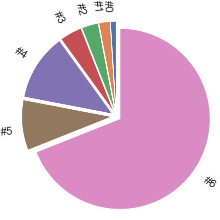
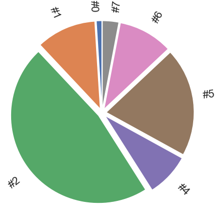
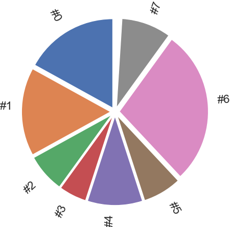
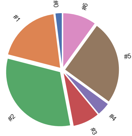
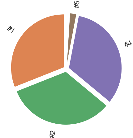
We evaluate the distributions of the experts being chosen to compute the nodes’ representations in the following. We set the number of experts to $8$. Figure 5 summarizes the relative frequencies of the experts being chosen on the datasets ZINC, ogbg-molhiv, and PATTERN. Generally, the performance of the shell attention heuristic degenerates whenever we observe expert collapsing. In the extreme case, just one expert expresses the mass of all nodes, and the capability to distribute learning nodes’ representations over several experts is not leveraged. To overcome expert collapsing, we can use a heuristic where in the early stages of the learning procedure, an additional epsilon parameter $\epsilon$ introduces randomness into the algorithm. Like a decaying greedy policy in Reinforcement Learning (RL), we choose a random expert with probability $\epsilon$ and choose the expert with the highest probability according to the routing layer with a probability of $1-\epsilon$. The epsilon value slowly decays over time. This ensures that all experts’ expressiveness is being explored to find the best matching one w.r.t to a node $u$ and prevents getting stuck in a local optimum. The figure shows the distribution of experts that are relevant for the computation of the nodes’ representations. For illustrative purposes, values below $1\%$ are omitted. Generally, nodes are more widely distributed over all available experts in the molecular datasets like ZINC and ogbg-molhiv for all models compared to PATTERN following a stochastic block model. Therefore, various experts are capable of capturing individual topological characteristics of molecules better than vanilla graph neural networks for which over-smoothing might potentially occur. We also observe that the mass is distributed to only a subset of the available experts for the PATTERN dataset. Hence, the specific number of iterations is more expressive for nodes within graph structures following SBM.

References

- Abbe (2018) Abbe, E. 2018. Community Detection and Stochastic Block Models. Found. Trends Commun. Inf. Theory, 14(1–2): 1–162.
- Beaini et al. (2020) Beaini, D.; Passaro, S.; Létourneau, V.; Hamilton, W. L.; Corso, G.; and Liò, P. 2020. Directional Graph Networks. CoRR, abs/2010.02863.
- Dwivedi and Bresson (2021) Dwivedi, V. P.; and Bresson, X. 2021. A Generalization of Transformer Networks to Graphs. arXiv:2012.09699.
- Dwivedi et al. (2020) Dwivedi, V. P.; Joshi, C. K.; Laurent, T.; Bengio, Y.; and Bresson, X. 2020. Benchmarking Graph Neural Networks. CoRR, abs/2003.00982.
- Fedus, Zoph, and Shazeer (2021) Fedus, W.; Zoph, B.; and Shazeer, N. 2021. Switch Transformers: Scaling to Trillion Parameter Models with Simple and Efficient Sparsity. CoRR, abs/2101.03961.
- Hamilton, Ying, and Leskovec (2017) Hamilton, W.; Ying, Z.; and Leskovec, J. 2017. Inductive Representation Learning on Large Graphs. In Guyon, I.; Luxburg, U. V.; Bengio, S.; Wallach, H.; Fergus, R.; Vishwanathan, S.; and Garnett, R., eds., Advances in Neural Information Processing Systems, volume 30. Curran Associates, Inc.
- Hoory, Linial, and Wigderson (2006) Hoory, S.; Linial, N.; and Wigderson, A. 2006. Expander Graphs and Their Applications. Bull. Amer. Math. Soc., 43(04): 439–562.
- Hu et al. (2020a) Hu, W.; Fey, M.; Zitnik, M.; Dong, Y.; Ren, H.; Liu, B.; Catasta, M.; and Leskovec, J. 2020a. Open Graph Benchmark: Datasets for Machine Learning on Graphs. arXiv preprint arXiv:2005.00687.
- Hu et al. (2020b) Hu, Z.; Dong, Y.; Wang, K.; and Sun, Y. 2020b. Heterogeneous Graph Transformer. In Proceedings of The Web Conference 2020, WWW ’20, 2704–2710. New York, NY, USA: Association for Computing Machinery. ISBN 9781450370233.
- Irwin et al. (2012) Irwin, J. J.; Sterling, T.; Mysinger, M. M.; Bolstad, E. S.; and Coleman, R. G. 2012. ZINC: A Free Tool to Discover Chemistry for Biology. Journal of chemical information and modeling, 52(7): 1757–1768.
- Kingma and Ba (2015) Kingma, D. P.; and Ba, J. 2015. Adam: A method for stochastic optimization. In International Conference on Learning Representations (ICLR).
- Kipf and Welling (2017) Kipf, T. N.; and Welling, M. 2017. Semi-Supervised Classification with Graph Convolutional Networks. In Proceedings of the 5th International Conference on Learning Representations, ICLR ’17.
- Kreuzer et al. (2021) Kreuzer, D.; Beaini, D.; Hamilton, W. L.; Létourneau, V.; and Tossou, P. 2021. Rethinking Graph Transformers with Spectral Attention. arXiv:2106.03893.
- Nguyen, Nguyen, and Phung (2019) Nguyen, D. Q.; Nguyen, T. D.; and Phung, D. 2019. Universal Self-Attention Network for Graph Classification. arXiv preprint arXiv:1909.11855.
- Paszke et al. (2019) Paszke, A.; Gross, S.; Massa, F.; Lerer, A.; Bradbury, J.; Chanan, G.; Killeen, T.; Lin, Z.; Gimelshein, N.; Antiga, L.; Desmaison, A.; Kopf, A.; Yang, E.; DeVito, Z.; Raison, M.; Tejani, A.; Chilamkurthy, S.; Steiner, B.; Fang, L.; Bai, J.; and Chintala, S. 2019. PyTorch: An Imperative Style, High-Performance Deep Learning Library. In Wallach, H.; Larochelle, H.; Beygelzimer, A.; d'Alché-Buc, F.; Fox, E.; and Garnett, R., eds., Advances in Neural Information Processing Systems, volume 32. Curran Associates, Inc.
- Rong et al. (2020) Rong, Y.; Bian, Y.; Xu, T.; Xie, W.; WEI, Y.; Huang, W.; and Huang, J. 2020. Self-Supervised Graph Transformer on Large-Scale Molecular Data. In Larochelle, H.; Ranzato, M.; Hadsell, R.; Balcan, M. F.; and Lin, H., eds., Advances in Neural Information Processing Systems, volume 33, 12559–12571. Curran Associates, Inc.
- Schwartz et al. (2020) Schwartz, R.; Dodge, J.; Smith, N. A.; and Etzioni, O. 2020. Green AI. Commun. ACM, 63(12): 54–63.
- Shazeer et al. (2017) Shazeer, N.; Mirhoseini, A.; Maziarz, K.; Davis, A.; Le, Q.; Hinton, G.; and Dean, J. 2017. Outrageously Large Neural Networks: The Sparsely-Gated Mixture-of-Experts Layer. arXiv preprint arXiv:1701.06538.
- Vaswani et al. (2017) Vaswani, A.; Shazeer, N.; Parmar, N.; Uszkoreit, J.; Jones, L.; Gomez, A. N.; Kaiser, u.; and Polosukhin, I. 2017. Attention is All You Need. In Proceedings of the 31st International Conference on Neural Information Processing Systems, NIPS’17, 6000–6010. Red Hook, NY, USA: Curran Associates Inc. ISBN 9781510860964.
- Veličković et al. (2017) Veličković, P.; Cucurull, G.; Casanova, A.; Romero, A.; Liò, P.; and Bengio, Y. 2017. Graph Attention Networks. 6th International Conference on Learning Representations.
- Wang et al. (2019) Wang, M.; Zheng, D.; Ye, Z.; Gan, Q.; Li, M.; Song, X.; Zhou, J.; Ma, C.; Yu, L.; Gai, Y.; Xiao, T.; He, T.; Karypis, G.; Li, J.; and Zhang, Z. 2019. Deep Graph Library: A Graph-Centric, Highly-Performant Package for Graph Neural Networks. arXiv preprint arXiv:1909.01315.
- Wu et al. (2021) Wu, Z.; Pan, S.; Chen, F.; Long, G.; Zhang, C.; and Yu, P. S. 2021. A Comprehensive Survey on Graph Neural Networks. IEEE Transactions on Neural Networks and Learning Systems, 32(1): 4–24.
- Xu et al. (2018a) Xu, K.; Hu, W.; Leskovec, J.; and Jegelka, S. 2018a. How Powerful are Graph Neural Networks? CoRR, abs/1810.00826.
- Xu et al. (2018b) Xu, K.; Hu, W.; Leskovec, J.; and Jegelka, S. 2018b. How Powerful are Graph Neural Networks? CoRR, abs/1810.00826.
- Ying et al. (2021) Ying, C.; Cai, T.; Luo, S.; Zheng, S.; Ke, G.; He, D.; Shen, Y.; and Liu, T.-Y. 2021. Do Transformers Really Perform Bad for Graph Representation? arXiv preprint arXiv:2106.05234.
- Yun et al. (2019) Yun, S.; Jeong, M.; Kim, R.; Kang, J.; and Kim, H. J. 2019. Graph Transformer Networks. In Wallach, H.; Larochelle, H.; Beygelzimer, A.; d'Alché-Buc, F.; Fox, E.; and Garnett, R., eds., Advances in Neural Information Processing Systems, volume 32. Curran Associates, Inc.
- Zhou et al. (2020) Zhou, D.; Zheng, L.; Han, J.; and He, J. 2020. A Data-Driven Graph Generative Model for Temporal Interaction Networks, 401–411. New York, NY, USA: Association for Computing Machinery. ISBN 9781450379984.