A generalised phase field model for fatigue crack growth in elastic-plastic solids with an efficient monolithic solver

Abstract

We present a generalised phase field-based formulation for predicting fatigue crack growth in metals. The theoretical framework aims at covering a wide range of material behaviour. Different fatigue degradation functions are considered and their influence is benchmarked against experiments. The phase field constitutive theory accommodates the so-called AT1, AT2 and phase field-cohesive zone (PF-CZM) models. In regards to material deformation, both non-linear kinematic and isotropic hardening are considered, as well as the combination of the two. Moreover, a monolithic solution scheme based on quasi-Newton algorithms is presented and shown to significantly outperform staggered approaches. The potential of the computational framework is demonstrated by investigating several 2D and 3D boundary value problems of particular interest. Constitutive and numerical choices are compared and insight is gained into their differences and similarities. The framework enables predicting fatigue crack growth in arbitrary geometries and for materials exhibiting complex (cyclic) deformation and damage responses. The finite element code developed is made freely available at www.empaneda.com/codes.

1 Introduction

Fatigue-induced fracture is considered to be one of the most frequent causes of failure in engineering components. Due to its complex nature, the development of computational models capable of predicting fatigue cracking is regarded to be highly challenging and has been the subject of extensive research. Generally, the evolution of fatigue damage occurs in different stages. Firstly, nucleation of permanent damage takes place as a result of sub- and microstructural changes within the material, followed by the creation of microscopic cracks. Subsequently, these microscopic flaws start growing and eventually coalescence, leading to the formation of dominant macro-cracks. These macro-cracks then propagate leading to structural instability and complete fracture of the component. Fatigue design is commonly based on classical empirical methods [1]. Such methods involve the estimation of the total life to failure as a function of the cyclic stress range, which is referred to as the S-N curve approach, or the strain range (plastic or total). These fatigue design strategies are commonly referred to as total-life approaches, where the fatigue life is defined as the number of cycles ($N_{f}$) or reversals ($2N_{f}$) to failure. The stress-life or S-N curve approach was first developed by Wöhler [2]. Under low cyclic stress amplitudes, the material behaves mainly in an elastic manner and a very large number of cycles are required to cause failure; normally more than 10⁶, which is referred to as High-cycle Fatigue (HCF). This approach has become popular in applications involving low-amplitude cyclic stresses such as steel bridges under traffic loading and railway axles. On the other hand, a much lower number of cycles are needed to cause failure if the applied stresses are large enough to cause plastic deformations; in the order of 10² to 10⁴, a regime referred to as Low-cycle Fatigue (LCF). In such situations, fatigue life is determined in terms of the applied strain range, as first proposed by Coffin [3] and Manson [4]. In the case of components experiencing very large plastic deformations, complete structural failure can occur after very few cycles [5, 6]. This is often referred to as Extremely- or Ultra-low Cycle fatigue (ELCF or ULCF). Due to their empirical nature, stress-life and strain-based approaches have limited applicability and cannot be readily generalised to arbitrary materials, geometries and loading histories.

Variational phase field fracture models can provide a reliable computational framework to predict High-, Low- and Extremely low-cycle fatigue, overcoming the limitations of semi-empirical approaches. Phase field fracture methods have been gaining increasing attention. Predictions are based on the thermodynamic framework outlined in the works of Griffith [7] and Irwin [8], where a crack would only propagate if the energy release rate exceeds a critical value, the material toughness $G_{c}$. Francfort and Marigo [9] introduced a variational formulation for Griffith’s thermodynamical framework, including the surface energy dissipated due to crack formation in the total potential energy. Inspired by the work of Mumford and Shah [10] on image segmentation, Bourdin et al. [11, 12] introduced a scalar phase field variable that regularises the discrete crack topology into a diffuse crack representation. In addition, Miehe and co-workers [13, 14] have made significant contributions to the development of the method by proposing new robust solution schemes.

Phase field fracture methods have been used in numerous applications, including dynamic fracture [15, 16, 17], cracking of composite materials [18, 19, 20, 21], ductile damage [22, 23, 24], hydrogen-assisted cracking [25, 26, 27, 28], and fracture of functionally graded materials [29, 30], among many others; see Refs. [31, 32] for an overview. Recently, the success of variational phase field methods has been extended to fatigue crack growth [33, 34, 35, 36, 37]. This is an exciting and natural extension for phase field fracture; Griffith’s thermodynamic principles should hold for fatigue crack growth and metal fatigue was actually the motivation for Griffith’s seminal work [7]. Lo et al. [34] combined a phase field kinetic law with a modified $J$-integral to capture Paris-law type fatigue crack growth behaviour. Carrara et al. [35] proposed a novel variational framework to capture the fatigue behaviour of brittle materials by introducing a fatigue degradation function that degrades the material toughness. Simoes and Martínez-Pañeda [36] simulated the fatigue failure of a NiTi stent, accounting for both fatigue damage and phase transformations. Hasan and Baxevanis [37] introduced a toughness degradation law through a measure of accumulated elastic strain energy density that enabled capturing both total life and defect tolerant approaches to fatigue. Golahmar et al. presented a phase field formulation for hydrogen assisted fatigue [38]. However, these studies are all limited to the analysis of linear elastic materials; only very recently have phase field methods been used to predict fatigue crack growth in elastic-plastic solids. Seiler et al. [39] used a local strain approach to empirically incorporate plasticity via Neuber’s rule. Haveroth et al. [40] presented a new thermo-mechanical fatigue formulation using a Voce-type hardening law and a new degradation function that degrades both elastic and plastic strain energy densities. Finally, Ulloa et al. [41] developed a phase field fatigue formulation for elastic-plastic solids suitable for both low and high cycle fatigue regimes and capable of capturing ratcheting effects.

In this work, we present a generalised formulation for fatigue damage in metals. We aim to model a general class of elastic-plastic materials and thus account for the combination of non-linear isotropic and kinematic hardening effects. Moreover, unlike previous work, we do not restrict our attention to one class of phase field fracture models but accommodate both brittle and quasi-brittle formulations; namely, the so-called AT1, AT2 and PF-CZM models. In addition, we couple our phase field fatigue framework with a quasi-Newton monolithic solution scheme and show that it is more robust and significantly more efficient than the widely-used staggered schemes. This is of notable importance given the computational cost associated with cycle-by-cycle fatigue predictions. Several 2D and 3D boundary value problems are investigated to gain insight into the various constitutive choices of the model for deformation and fracture. Firstly, we simulate the fatigue failure of planar specimens under uniaxial cyclic loading. Predictions are compared with experiments on a carbon steel that exhibits combined non-linear isotropic and kinematic hardening. Secondly, fatigue crack growth in a Compact Tension (CT) sample is investigated, evaluating the differences between various phase field fracture models and solution schemes. Thirdly, the failure of an asymmetrically-notched bar is simulated to gain insight into the interplay between hardening mechanisms and damage. Finally, we demonstrate the capabilities of the computational framework in predicting the failure of 3D components by modelling crack nucleation and growth in a pipe-to-pipe connection.

The remainder of this manuscript is organised as follows. The generalised theoretical framework presented is described in Section 2. In Section 3 we provide details of the numerical implementation, including the monolithic quasi-Newton solution scheme. The results computed are shown and discussed in Section 4. Finally, the manuscript ends with concluding remarks in Section 5.

2 Theory

In this section, we present our generalised formulation, suitable for arbitrary constitutive choices of crack density function, fracture driving force, degradation function and cyclic material response. The theory refers to an elastic-plastic body occupying an arbitrary domain $\Omega\subset{\rm I\!R}^{n}$ $(n\in[1,2,3])$, with an external boundary $\partial\Omega\subset{\rm I\!R}^{n-1}$, on which the outwards unit normal is denoted as $\mathbf{n}$. We shall first define the kinematic variables (Section 2.1), then derive the force balances using the principle of virtual power (Section 2.2), and finally particularise our theory to relevant constitutive choices for the deformation and fracture behaviour of the solid (Section 2.3).

2.1 Kinematics

The primary kinematic variables are the displacement field vector $\mathbf{u}$ and the damage phase field $\phi$. Small displacements and strains are assumed, such that the total strain tensor $\bm{\varepsilon}$ reads

$$\bm{\varepsilon}=\frac{1}{2}\left(\nabla\mathbf{u}^{T}+\nabla\mathbf{u}\right)\,.$$ (1)

Also, we adopt the standard decomposition of strains into elastic and plastic components, such that:

$$\bm{\varepsilon}=\bm{\varepsilon}^{e}+\bm{\varepsilon}^{p}\,.$$ (2)

The nucleation and growth of cracks are described by using a smooth continuous scalar phase field $\phi\in[0;1]$. The use of an auxiliary phase field variable to implicitly track interfaces has proven to be a very compelling computational approach for numerous interfacial problems, such as microstructural evolution [42] and metallic corrosion [43]. In the context of fracture mechanics, the phase field variable resembles a damage variable; it must grow monotonically $\dot{\phi}(\mathbf{x},t)\geq 0$ and describes the degree of damage, with $\phi=1$ denoting fracture and $\phi=0$ corresponding to the intact phase. Since $\phi$ is smooth and continuous, discrete cracks are represented in a diffuse fashion, with the smearing of cracks being controlled by a phase field length scale $\ell$. The aim of this diffuse representation is to introduce, over a discontinuous surface $\Gamma$, the following approximation of the fracture energy [11]:

$$\Phi=\int_{\Gamma}G_{c}\,\text{d}S\approx\int_{\Omega}G_{c}\Upsilon(\phi,\nabla\phi)\,\text{d}V,\hskip 28.45274pt\text{for }\ell\rightarrow 0^{+},$$ (3)

where $\Upsilon$ is the so-called crack surface density functional and $G_{c}$ is the critical energy release rate or material toughness. We extend this rate-independent description of fracture to accommodate time and history dependent problems. Thus, for a cumulative history variable $\bar{\vartheta}$, which fulfills $\dot{\bar{\vartheta}}>0$, and a fatigue degradation function $f\left(\bar{\vartheta}\right)$, the fracture energy can be re-formulated as follows,

$$\Phi=\int_{0}^{t}\left(\int_{\Omega}G_{c}f\left(\bar{\vartheta}\left(t\right)\right)\dot{\Upsilon}(\phi,\nabla\phi)\,\text{d}V\right)\,\text{d}t\,.$$ (4)

As described below, this is complemented by appropriate constitutive choices that characterise the degradation of the fracture energy with the fatigue history variable $\bar{\vartheta}$.

2.2 Principle of virtual power. Balance of forces

Now, let us derive the balance equations for the coupled deformation-fatigue system using the principle of virtual power. Define $\bm{\sigma}$ as the symmetric Cauchy tensor, $\mathbf{T}$ as a surface traction acting on the boundary of the solid $\partial\Omega$ and $\mathbf{b}$ as a prescribed body force per unit volume. With respect to the damage problem, we introduce a scalar stress-like quantity $\omega$, which is work conjugate to the phase field $\phi$, and a phase field micro-stress vector $\bm{\upxi}$, which is work conjugate to the gradient of the phase field $\nabla\phi$. No external traction is associated with the phase field. We define the kinematics of the body $\Omega$ using the fields $\mathbf{u}$ and $\phi$. The corresponding velocities read $\dot{\mathbf{u}}$ and $\dot{\phi}$, while the virtual velocities, defined over a vector space $\mathcal{V}$, are denoted by $\tilde{\mathbf{u}}$ and $\tilde{\phi}$ [44, 45, 46]. Accordingly, the principle of virtual power reads:

$$\int_{\Omega}\left[\bm{\sigma}:\nabla\tilde{\mathbf{u}}+\omega\tilde{\phi}+\bm{\upxi}\cdot\nabla\tilde{\phi}\right]\,\text{d}V=\int_{\partial\Omega}\left(\mathbf{T}\cdot\tilde{\mathbf{u}}\right)\,\text{d}S+\int_{\Omega}\left(\mathbf{b}\cdot\tilde{\mathbf{u}}\right)\,\text{d}V\,.$$ (5)

By application of the Gauss divergence theorem and the fundamental lemma of calculus of variations, the local force balances are given by:

$$\begin{split}&\nabla\cdot\bm{\sigma}+\mathbf{b}=0\\ &\nabla\cdot\bm{\upxi}-\omega=0\end{split}\hskip 56.9055pt\text{in }\,\,\Omega,$$ (6)

with natural boundary conditions:

$$\begin{split}\bm{\sigma}\cdot\mathbf{n}=\mathbf{T}\\ \bm{\upxi}\cdot\mathbf{n}=0\end{split}\hskip 56.9055pt\text{on }\,\,\partial\Omega.$$ (7)

2.3 Constitutive theory

We shall now proceed to make suitable constitutive choices for the deformation, fracture and fatigue behaviour of the solid. First, we define the total potential energy of the solid as the sum of the strain energy density of the solid $\psi$ and the fracture energy density $\varphi$, such that:

$$W\left(\bm{\varepsilon}\left(\mathbf{u}\right),\,\phi,\,\nabla\phi\right)=\psi\left(\bm{\varepsilon}\left(\mathbf{u}\right),\,g\left(\phi\right)\right)+\varphi\left(\phi,\,\nabla\phi\right)\,,$$ (8)

where $g\left(\phi\right)$ is a phase field degradation function, to be defined. The Cauchy stress tensor is then defined as $\bm{\sigma}=\partial_{\bm{\varepsilon}}\psi$. Thus, the phase field reduces the stiffness of the solid. However, note that no damage-plasticity coupling term is defined. The reader is referred to Alessi et al. [47] for a comprehensive discussion on potential constitutive choices to capture the interplay between damage and elastic-plastic material behaviour. The strain energy density includes both elastic and plastic parts, which are computed as follows:

$$\psi_{0}=\psi^{e}\left(\bm{\varepsilon}^{e}\right)+\psi^{p}\left(\bm{\varepsilon}^{p}\right)=\frac{1}{2}\lambda\left[\text{tr}\left(\bm{\varepsilon}^{e}\right)\right]^{2}+\mu\,\text{tr}\left[\left(\bm{\varepsilon}^{e}\right)^{2}\right]+\int_{0}^{t}\left(\bm{\sigma}_{0}:\dot{\bm{\varepsilon}}^{p}\right)\text{d}t\,,$$ (9)

where $\lambda$ and $\mu$ are the Lamé parameters and the subscript $0$ denotes an undamaged quantity. In agreement with (4), the fracture energy density is defined as,

$$\varphi=f\left(\bar{\vartheta}\right)G_{c}\Upsilon(\phi,\nabla\phi)=f\left(\bar{\vartheta}\right)\dfrac{G_{c}}{4c_{w}\ell}\left(w(\phi)+\ell^{2}|\nabla\phi|^{2}\right)\,.$$ (10)

Here, $w(\phi)$ is the geometric crack function, to be defined, and $c_{w}$ is a scaling constant, given by

$$c_{w}=\int_{0}^{1}\sqrt{w(\zeta)}\,\text{d}\zeta\,.$$ (11)

2.3.1 Strain energy decomposition

To prevent the nucleation and growth of cracks under compression, the strain energy density can be decomposed into tensile and compressive parts as follows:

$$\psi\left(\bm{\varepsilon}^{e},\bm{\varepsilon}^{p},\phi\right)=g\left(\phi\right)\left(\psi_{+}^{e}\left(\bm{\varepsilon}^{e}\right)+\psi^{p}\left(\bm{\varepsilon}^{p}\right)\right)+\psi^{e}_{-}\left(\bm{\varepsilon}^{e}\right)\,.$$ (12)

We choose to follow the so-called volumetric-deviatoric split proposed by Amor et al. [48]. Accordingly, for a material with bulk modulus $K$, the elastic strain energy density is decomposed as,

$$\psi^{e}_{+}\left(\bm{\varepsilon}\right)=\frac{1}{2}K\langle\text{tr}\left(\bm{\varepsilon}^{e}\right)\rangle^{2}_{+}+\mu\left({\bm{\varepsilon}^{e}}^{\prime}:{\bm{\varepsilon}^{e}}^{\prime}\right)\,,\,\,\,\,\,\,\psi^{e}_{-}\left(\bm{\varepsilon}^{e}\right)=\frac{1}{2}K\langle\text{tr}\left(\bm{\varepsilon}^{e}\right)\rangle^{2}_{-}\,,$$ (13)

where ${\bm{\varepsilon}^{e}}^{\prime}$ denotes the deviatoric part of the elastic strain tensor and $\langle\,\rangle$ are the Macaulay brackets.

2.3.2 Karush–Kuhn–Tucker (KKT) conditions

Damage is an irreversible process and, as a consequence, the phase field evolution law must fulfill the condition $\dot{\phi}\geq 0$. To achieve this, we follow Miehe and co-workers [13, 14] and define a history variable field $\mathcal{H}$. Since the effective plastic work is assumed to increase monotonically, the history field variable only relates to the elastic fracture driving force, $\psi_{+}^{e}$. Thus, as dictated by the Karush–Kuhn–Tucker (KKT) conditions, the definition of $\mathcal{H}$ must satisfy:

$$\psi_{+}^{e}-\mathcal{H}\leq 0\text{,}\hskip 22.76219pt\dot{\mathcal{H}}\geq 0\text{,}\hskip 22.76219pt\dot{\mathcal{H}}(\psi_{+}^{e}-\mathcal{H})=0\,\,.\centering\@add@centering$$ (14)

Accordingly, for a current time $t$, within a total time $t_{t}$, we define the history field as,

$$\mathcal{H}=\text{max}_{t\in[0,t_{t}]}\psi_{+}^{e}\left(t\right)\,.$$ (15)

2.3.3 Fatigue damage

The damage resulting from the application of cyclic loads is captured by means of a fatigue degradation function $f(\bar{\vartheta})$, a cumulative history variable $\bar{\vartheta}$, and a fatigue threshold parameter $\vartheta_{T}$. We follow the work by Carrara et al. [35] on elastic solids and consider two fatigue degradation functions; one of an asymptotic form:

$${f}(\bar{\vartheta}(t))=\begin{cases}1&\text{if }\bar{\vartheta}(t)\leq\vartheta_{T}\\ \left(\frac{2\vartheta_{T}}{\bar{\vartheta}(t)+\vartheta_{T}}\right)^{2}&\text{if }\bar{\vartheta}(t)\geq\vartheta_{T}\end{cases}$$ (16)

and a second one, of logarithmic form:

$${f}(\bar{\vartheta}(t))=\begin{cases}1&\text{if }\bar{\vartheta}(t)\leq\vartheta_{T}\\ \left[1-\kappa\text{log}\left(\frac{\bar{\vartheta}(t)}{\vartheta_{T}}\right)\right]^{2}&\text{if }\vartheta_{T}\leq\bar{\vartheta}(t)\leq\vartheta_{T}10^{1/\kappa}\\ 0&\text{if }\bar{\vartheta}(t)\geq\vartheta_{T}10^{1/\kappa}\end{cases}$$ (17)

where $\kappa$ is a material parameter that characterises the slope of the logarithmic function. The impact of these choices must be assessed against experiments. Here, we provide a comparison against testing data on hot-rolled structural steels (see Section 4.1). In addition, the evolution of the fatigue history variable $\bar{\vartheta}$ is given by,

$$\bar{\vartheta}(t)=\int_{0}^{t}H(\vartheta\dot{\vartheta})|\dot{\vartheta}|\text{ d}t\,,$$ (18)

where $H(\vartheta\dot{\vartheta})$ is the Heaviside function such that $\bar{\vartheta}$ only evolves during loading.

Finally, it remains to define the fatigue threshold parameter $\vartheta_{T}$ and the fatigue history variable $\vartheta$. For the latter, we choose to adopt the following constitutive choice,

$$\vartheta=g\left(\phi\right)\left(\mathcal{H}+\psi^{p}\right)\,,$$ (19)

which implies that fatigue damage is driven by both elastic and plastic straining. This choice is consistent with the definition of a fracture driving force driven by both elastic and plastic strain energy densities. However, note that the use of the history field (as opposed to $\psi_{+}^{e}$) aims at minimising the elastic contribution, as arguably appropriate in the context of low-cycle fatigue. For the fatigue threshold, we follow Carrara et al. [35] and assume:

$$\vartheta_{T}=\frac{G_{c}}{12\ell}\,,$$ (20)

unless otherwise stated.

2.3.4 Micro-force variables

We proceed to derive, without loss of generality, the fracture micro-stress variables $\omega$ and $\bm{\upxi}$. First, considering (8), (9) and (15), we reformulate the total potential energy of the solid as,

$$W={g(\phi)}\left(\mathcal{H}+\psi^{p}\right)+f\left(\bar{\vartheta}\right)\frac{G_{c}}{4c_{w}}\left(\frac{w(\phi)}{\ell}+\ell|\nabla\phi|^{2}\right)\,.$$ (21)

Consequently, the scalar micro-stress $\omega$ is defined as:

$$\omega=\dfrac{\partial W}{\partial\phi}={g^{\prime}(\phi)}\left(\mathcal{H}+\psi^{p}\right)+f\left(\bar{\vartheta}\right)\frac{G_{c}}{4c_{w}\ell}w^{\prime}(\phi)\,,$$ (22)

and the phase field micro-stress vector $\bm{\upxi}$ reads,

$$\bm{\upxi}=\dfrac{\partial W}{\partial\nabla\phi}=\frac{\ell}{2c_{w}}G_{\mathrm{c}}f\left(\bar{\vartheta}\right)\nabla\phi\,.$$ (23)

The phase field evolution law (6b) can be reformulated by taking into consideration the constitutive relations (22) and (23), such that

$$\frac{G_{c}f\left(\bar{\vartheta}\right)}{2c_{w}}\left(\frac{w^{\prime}(\phi)}{2\ell}-\ell\nabla^{2}\phi\right)-\frac{G_{c}\ell}{2c_{w}}\nabla\phi\nabla f\left(\bar{\vartheta}\right)+{g^{\prime}(\phi)}\left(\mathcal{H}+\psi^{p}\right)=0\,.$$ (24)

It is evident from (15) and (24) that the phase field evolution is driven by both elastic and plastic strain energy densities. This is in agreement with several phase field models for fracture in elastic-plastic solids [49, 23, 50]. However, other approaches have also been considered in the literature (see, e.g. [45, 51]) and the choice is not straightforward. From a thermodynamical perspective, the majority of the energy stored in the solid (and thus available to facilitate crack growth) is elastic. However, failure in ductile fracture experiments is often driven by plastic phenomena and a simple energy balance is not suitable for crack growth processes involving significant plasticity; e.g., the assumption of an isothermal process is no longer valid as plastic flow constitutes a source of heat [32].

2.3.5 Degradation and dissipation functions

Now, we particularise our generalised framework by making specific choices for the fracture degradation function $g(\phi)$, the so-called dissipation function $w(\phi)$ [52, 33, 53] and the fracture driving force threshold $\mathcal{H}_{min}$. Our theory captures both brittle and quasi-brittle phase field approaches, accommodating the so-called AT1, AT2 and PF-CZM models. The AT1 and AT2 models are based on the Ambrosio and Tortorelli regularisaton of the Mumford-Shah functional [54, 11], with the former aimed at including a purely elastic response up to the onset of damage [55]. The phase field cohesive zone model PF-CZM employed here is inspired by the work by Wu [56] and Wu and Nguyen [57], but it employs a fracture driving force based on the strain energy density, as in Ref. [16]. In other words, fracture is driven by both elastic and plastic strain energy densities in the three phase field models considered, as shown in (24).

Firstly, we start by defining the phase field degradation function, which should satisfy:

$$g\left(0\right)=1,\,\,\,\,\,\,\,\,\,\,g\left(1\right)=0,\,\,\,\,\,\,\,\,\,\,g^{\prime}\left(\phi\right)\leq 0\,\,\,\text{for}\,\,\,0\leq\phi\leq 1\,.$$ (25)

For the AT1 and AT2 models the same choice is adopted; a quadratic degradation function such that,

$$g\left(\phi\right)=\left(1-\phi\right)^{2}\,.$$ (26)

While for the PF-CZM model, the following form is used,

$$g\left(\phi\right)=\frac{\left(1-\phi\right)^{2}}{\left(1-\phi\right)^{2}+m\phi\left(1-0.5\phi\right)}\,\,\,\,\,\,\,\text{with}\,\,\,\,\,\,\,m=\frac{3EG_{c}}{2\ell\sigma_{c}^{2}}\,,$$ (27)

where $\sigma_{c}$ is the material strength.

Secondly, we define the dissipation function, which should fulfill the following conditions:

$$w\left(0\right)=0,\,\,\,\,\,\,\,\,\,\,w\left(1\right)=1,\,\,\,\,\,\,\,\,\,\,w^{\prime}\left(\phi\right)\geq 0\,\,\,\text{for}\,\,\,0\leq\phi\leq 1\,.$$ (28)

The specific choice $w(\phi)=\phi^{2}$ ($c=1/2$) recovers the AT2 model while $w(\phi)=\phi$ ($c=2/3$) renders the AT1 formulation. No threshold for damage exists in the AT2 case as $w^{\prime}(0)=0$, unlike in the AT1 model. Finally, for the PF-CZM we have $w(\phi)=4\phi$ ($c_{w}=4/3$), where $w^{\prime}(0)>0$ - as in the AT1 case. Accordingly, a damage threshold should be defined for both AT1 and PF-CZM models; the following choices are adopted here,

$$\texttt{AT1}:\,\,\,\mathcal{H}_{min}=\frac{3G_{c}}{16\ell}\,,\,\,\,\,\,\,\,\,\,\,\,\texttt{PF-CZM}:\,\,\,\mathcal{H}_{min}=\frac{\sigma_{c}^{2}}{2E}\,.$$ (29)

Accordingly, in the numerical implementation of the AT1 and PF-CZM models, the history field is taken to be the maximum of (15) and $\mathcal{H}_{min}$.

It is also important to note that the PF-CZM model explicitly incorporates the material strength $\sigma_{c}$ into the constitutive equations - see (27) and (29)b. For the AT1 and AT2, a relation between the strength and the phase field length scale can be derived by considering the homogeneous solution to the phase field evolution law (see, e.g. Ref. [32]):

$$\texttt{AT1}:\,\,\,\sigma_{c}=\sqrt{\frac{3EG_{c}}{8\ell}}\,,\,\,\,\,\,\,\,\,\,\,\,\texttt{AT2}:\,\,\,\sigma_{c}=\frac{3}{16}\sqrt{\frac{3EG_{c}}{\ell}}\,.$$ (30)

2.3.6 Cyclic deformation: combined isotropic/kinematic hardening

The constitutive choices for relating the stresses to the strains aim at modelling a general class of elastic-plastic materials. Specifically, a nonlinear combined isotropic/kinematic hardening model is used to capture a wide range of cyclic plasticity phenomena. The model is based on the work by Lemaitre and Chaboche [58], where a von Mises yield criterion is combined with a non-linear description of isotropic and kinematic hardening effects.

For a material with current yield stress $\sigma_{Y}$, experiencing a deviatoric backstress $\bm{\alpha}^{\prime}$, the assumed yield function reads,

$$\mathcal{F}=\sqrt{\frac{2}{3}\left(\bm{\sigma}^{\prime}-\bm{\alpha}^{\prime}\right):\left(\bm{\sigma}^{\prime}-\bm{\alpha}^{\prime}\right)}-\sigma_{Y}=0\,,$$ (31)

where the first term is the von Mises effective stress. The flow rule then reads,

$$\dot{\bm{\varepsilon}}^{p}=\dot{\varepsilon}^{p}\frac{\partial\mathcal{F}}{\partial\bm{\sigma}}$$ (32)

where $\dot{\varepsilon}^{p}$ is the equivalent plastic strain rate, defined as $\dot{\varepsilon}^{p}=\sqrt{(2/3)\dot{\bm{\varepsilon}}^{p}:\dot{\bm{\varepsilon}}^{p}}$.

The hardening evolution law includes two components: an isotropic hardening one, describing the change in size of the yield surface, and a kinematic hardening one, characterising the translation of the yield surface in the stress space. We employ an exponential isotropic hardening law to relate the change in yield stress to the equivalent plastic strain $\varepsilon^{p}$ and the initial yield stress $\sigma_{0}$ as,

$$\sigma_{Y}=\sigma_{0}+Q_{\infty}\left[1-\exp{\left(-b\varepsilon^{p}\right)}\right]\,,$$ (33)

where $Q_{\infty}$ is the maximum change in the size of the yield surface and $b$ determines the rate at which the size of the yield surface changes as the plastic strain develops. On the other side, kinematic hardening effects are captured by means of an additive combination of a purely kinematic term, as in Ziegler’s linear hardening law [59], and a relaxation term, which introduces the non-linearity. The model can accommodate several superposed backstresses, which can improve predictions. Accordingly, for each backstress component,

$$\dot{\bm{\alpha}}_{k}=\frac{C_{k}}{\sigma_{Y}}\left(\bm{\sigma}-\bm{\alpha}\right)\dot{\varepsilon}^{p}-\gamma_{k}\bm{\alpha}_{k}\dot{\varepsilon}^{p}\,\,\,\,\,\,\,\,\,\text{with}\,\,\,\,\,\,\,\,\,\bm{\alpha}=\sum_{k=1}^{\mathcal{N}}\bm{\alpha}_{k}\,,$$ (34)

where $C$ and $\gamma$ are parameters calibrated against experimental data from a stabilised stress-strain cycle, and $\mathcal{N}$ is the number of backstresses. Note that the maximum change in backstress is controlled by the ratio $C/\gamma$, where $\gamma$ specifies the rate at which the backstress changes as the plastic strain develops. The model reduces to Ziegler’s linear hardening law when $\bm{\alpha}_{k}=0$ and to an isotropic hardening model when both $C_{k}$ and $\gamma_{k}$ are zero. On the other hand, a purely (non-linear) kinematic hardening model is recovered if $\sigma_{Y}=\sigma_{0}$. The one-dimensional representation of the non-linear combined isotropic-kinematic hardening law assumed is shown in Fig. 1. The maximum uniaxial stress attained is denoted by $\sigma^{max}$ and $\alpha_{s}$ corresponds to the magnitude of the backstress at saturation.

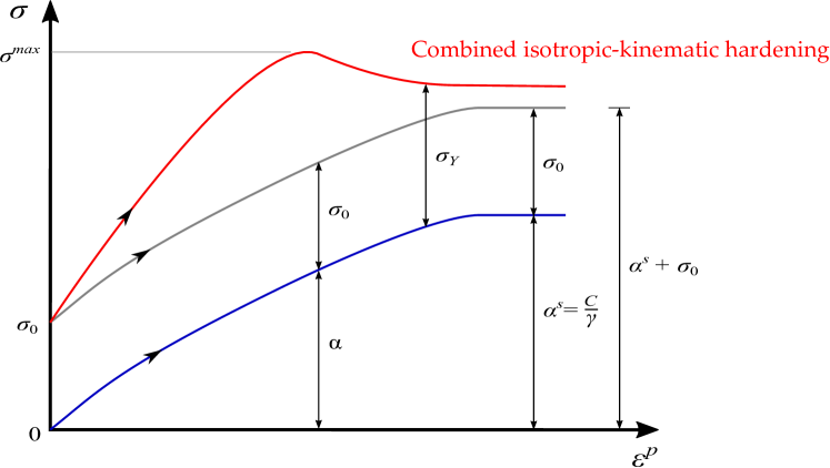
Figure 1: Sketch of the stress versus plastic strain response under uniaxial loading to illustrate the nonlinear combined isotropic/kinematic hardening model.

3 Numerical implementation

Details of the numerical implementation are provided here, starting with the finite element discretisation (Section 3.1), followed by the formulation of the residuals and the stiffness matrices (Section 3.2), and ending with a description of the quasi-Newton algorithm employed to enable an efficient and robust monolithic implementation (Section 3.3). The theoretical framework outlined in Section 2 is numerically implemented in the commercial finite element package ABAQUS by developing a user-defined UELMAT subroutine, this is described in Section 3.4.

3.1 Finite element discretisation

Making use of Voigt notation, the primal kinematic variables of the problem are discretised in terms of their nodal values $\textbf{u}_{i}=\{u_{x},u_{y},u_{z}\}^{T}$ and $\phi_{i}$ at node $i$ as:

$$\textbf{u}=\sum_{i=1}^{m}\bm{N}_{i}^{\textbf{u}}\textbf{u}_{i}\text{\hskip 28.45274ptand\hskip 28.45274pt}\phi=\sum_{i=1}^{m}N_{i}\phi_{i}$$ (35)

where $m$ is the total number of nodes per element, $N_{i}$ is the shape function associated with node $i$ and $\bm{N}_{i}^{\textbf{u}}$ is the shape function matrix, a diagonal matrix with $N_{i}$ in the diagonal terms. Making use of the corresponding $\bm{B}$-matrices, which contain the derivatives of the shape functions, the discretised derivatives of u and $\phi$ can be expressed as follows,

$$\boldsymbol{\varepsilon}=\sum_{i=1}^{m}\bm{B}_{i}^{\textbf{u}}\textbf{u}_{i}\text{\hskip 28.45274ptand\hskip 28.45274pt}\nabla\phi=\sum_{i=1}^{m}\textbf{B}_{i}^{\phi}\phi_{i}\,.$$ (36)

3.2 Residuals and stiffness matrices

Let us now formulate the weak form of the problem. Considering the principle of virtual power (5) and the constitutive choices described in Section 2, the weak form of the displacement and phase field problems read:

$$\int_{\Omega}\Big{\{}\big{[}{g(\phi)}+\varkappa\big{]}\bm{\sigma}_{0}:\text{sym}\nabla\delta\mathbf{u}-\mathbf{b}\cdot\delta\mathbf{u}\Big{\}}\,\text{d}V+\int_{\partial\Omega}\mathbf{T}\cdot\delta\mathbf{u}\,\text{d}S=0\,,$$ (37)

$$\int_{\Omega}\left\{{g^{\prime}(\phi)\delta\phi}\,\left(\mathcal{H}+\psi^{p}\right)+\frac{G_{c}}{2c_{w}}f\left(\bar{\vartheta}\right)\left[\frac{w^{\prime}(\phi)}{2\ell}\delta\phi-\ell\nabla\phi\nabla\delta\phi\right]\right\}\,\mathrm{d}V=0\,.$$ (38)

Here, $\bm{\sigma}_{0}$ is the undamaged stress tensor and $\varkappa$ is a small, positive constant used to prevent ill-conditioning when $\phi=1$; in this work, $\varkappa=1\times 10^{-7}$. Also, note that a hybrid approach is used, by which the strain energy density split is only applied to the phase field balance but with $\phi$ degrading the total strain energy density in the linear momentum balance equation [60]. Now, introduce the discretisation outlined in (35)-(36) into the weak form to derive the corresponding residuals:

$$\mathbf{R}_{i}^{\mathbf{u}}=\int_{\Omega}\left\{\left[{g(\phi)}+\varkappa\right]\left(\bm{B}^{\mathbf{u}}_{i}\right)^{T}\bm{\sigma}_{0}-\left(\bm{N}_{i}^{\mathbf{u}}\right)^{T}\mathbf{b}\right\}\,\text{d}V-\int_{\partial\Omega}\left(\bm{N}_{i}^{\mathbf{u}}\right)^{T}\mathbf{T}\,\text{d}S\,,$$ (39)

$$R_{i}^{\phi}=\int_{\Omega}\left\{{g^{\prime}(\phi)}N_{i}\left(\mathcal{H}+\psi^{p}\right)+\frac{G_{c}}{2c_{w}\ell}f\left(\bar{\vartheta}\right)\left[\frac{w^{\prime}(\phi)}{2}N_{i}+\ell^{2}\,\left(\mathbf{B}_{i}\right)^{T}\nabla\phi\right]\right\}dV\,.$$ (40)

Finally, we obtain the consistent tangent stiffness matrices $\bm{K}$ by differentiating the residuals with respect to the incremental nodal variables as follows:

$$\bm{K}_{ij}^{\mathbf{u}}=\frac{\partial\bm{R}_{i}^{\bm{u}}}{\partial\bm{u}_{j}}=\int_{\Omega}\left\{\left[{g(\phi)}+\varkappa\right]{(\bm{B}_{i}^{\bm{u}})}^{T}\bm{C}_{ep}\,\bm{B}_{j}^{\bm{u}}\right\}\,\text{d}V\,,$$ (41)

$$\bm{K}_{ij}^{\phi}=\frac{\partial R_{i}^{\phi}}{\partial\phi_{j}}=\int_{\Omega}\left\{\left({g^{\prime\prime}(\phi)}\left(\mathcal{H}+\psi^{p}\right)+\frac{G_{c}f\left(\bar{\vartheta}\right)}{4c_{w}\ell}{w^{\prime\prime}(\phi)}\right)N_{i}N_{j}+f\left(\bar{\vartheta}\right)\frac{G_{c}\ell}{2c_{w}}\,\mathbf{B}_{i}^{T}\mathbf{B}_{j}\right\}\,\text{d}V\,,$$ (42)

where $\bm{C}_{ep}$ is the elastic-plastic material Jacobian. The global system of equations then reads,

$${\begin{bmatrix}\textbf{K}^{\textbf{uu}}&0\\ 0&\textbf{K}^{\phi\phi}\end{bmatrix}}\begin{Bmatrix}\textbf{r}^{\textbf{u}}\\ \textbf{r}^{\phi}\end{Bmatrix}=\begin{Bmatrix}\textbf{u}\\ \phi\end{Bmatrix}$$ (43)

The u and $\phi$ solutions can be obtained monolithically (simultaneously) or following a staggered (sequential) approach. Staggered solution schemes have been traditionally considered more robust but come at the cost of losing unconditional stability, requiring the use of sufficiently small load increments to ensure that the solution does not deviate from the equilibrium one. This can be a significant bottleneck for phase field fatigue calculations, where errors can accumulate in every cycle. We will show how a robust and efficient monolithic solution scheme can be achieved by using quasi-Newton methods, such as the Broyden-Fletcher-Goldfarb-Shanno (BFGS) algorithm [61, 62], enabling accurate fatigue crack growth estimations. Note that, a requirement of the BFGS algorithm described below is that the stiffness matrix is symmetric and positive-definite. Hence, $\textbf{K}^{\textbf{u}\phi}=\textbf{K}^{\phi\textbf{u}}=0$.

3.3 A quasi-Newton solution scheme: the BFGS algorithm

Quasi-Newton methods have proven to be very robust when dealing with non-convex minimisation problems (see, e.g. [63, 64] and Refs. therein). As opposed to standard Newton approaches, the stiffness matrix $\mathbf{K}$ is not updated after each iteration in quasi-Newton algorithms. Instead, an approximation of the stiffness is introduced after a given number of iterations without convergence. This approximated stiffness matrix, $\tilde{\mathbf{K}}$, satisfies:

$$\tilde{\mathbf{K}}\Delta\mathbf{z}=\Delta\mathbf{r}\,\,\,\,\,\,\,\,\,\text{with}\,\,\,\,\,\,\,\,\,\mathbf{z}=\begin{Bmatrix}\mathbf{u}\\[3.00003pt] \bm{\phi}\end{Bmatrix}\,,$$ (44)

Here, $\Delta\mathbf{z}=\mathbf{z}_{t+\Delta t}-\mathbf{z}_{t}$ and $\Delta\mathbf{r}=\mathbf{r}_{t+\Delta t}-\mathbf{r}_{t}$. We choose to adopt the BFGS algorithm, in which the approximated stiffness matrix is typically defined as [65],

$$\tilde{\mathbf{K}}=\tilde{\mathbf{K}}_{t}-\dfrac{(\tilde{\mathbf{K}}_{t}\Delta\mathbf{z})(\tilde{\mathbf{K}}_{t}\Delta\mathbf{z}{)}^{T}}{\Delta\mathbf{z}\tilde{\mathbf{K}}_{t}\Delta\mathbf{z}}+\dfrac{\Delta\mathbf{r}\Delta\mathbf{r}^{T}}{\Delta\mathbf{z}^{T}\Delta\mathbf{r}}$$ (45)

From a computational perspective, and upon the assumption of a symmetric stifness matrix, the approximated stiffness matrix can be expressed as follows [66],

$$\tilde{\mathbf{K}}^{-1}=\left(\mathbf{I}-\dfrac{\Delta\mathbf{z}\Delta\mathbf{r}^{T}}{\Delta\mathbf{z}^{T}\Delta\mathbf{r}}\right)\tilde{\mathbf{K}}_{t}^{-1}\left(\mathbf{I}-\dfrac{\Delta\mathbf{z}\Delta\mathbf{r}^{T}}{\Delta\mathbf{z}^{T}\Delta\mathbf{r}}\right)^{-1}+\dfrac{\Delta\mathbf{z}\Delta\mathbf{z}^{T}}{\Delta\mathbf{z}^{T}\Delta\mathbf{r}}\,.$$ (46)

In this way, symmetry and positive definiteness are retained. As it can be observed, if the initial guess is symmetric and positive definite, as in (43), the updated $\tilde{\mathbf{K}}$ is also symmetric and positive definite. The BFGS algorithm has been implemented in most commercial finite element packages (such as ABAQUS), often in conjunction with a line search algorithm.

3.4 Details of the ABAQUS implementation

A UELMAT subroutine is used to implement the generalised model into the commercial finite element package ABAQUS. The UELMAT, similar to user element (UEL) subroutines, requires defining the element residual and stiffness matrices, such that the coding resembles that of an in-house code (ABAQUS is solely used to assemble the global matrices and solve the system). However, the UELMAT differs from the UEL in that it enables access to the ABAQUS’s material library (material_lib_mech). We exploit this to obtain $\bm{\sigma}_{0}$ and $\bm{C}_{ep}$ for a given strain tensor. In addition, we use the elastic compliance tensor to decompose the total strains into their elastic and plastic counterparts.

4 Results

We proceed to showcase the capabilities of the computational framework presented by addressing several boundary value problems of particular interest. Firstly, in Section 4.1, the number of cycles to failure is estimated under uniaxial cyclic loading and compared with experimental predictions on structural steels. This is accompanied by a parametric study to evaluate the role of the various fracture and fatigue parameters of the model. Secondly, fatigue crack growth in a Compact Tension specimen is predicted, for different solution schemes and phase field models (Section 4.2). Thirdly, in Section 4.3, the interplay between damage and isotropic and kinematic hardening effects is examined in an asymmetrically-notched bar. Finally, we simulate the structural failure of a pipe-to-pipe connection to showcase the capabilities of the model for delivering large scale, 3D predictions (Section 4.4).

4.1 Uniaxial tension-compression experiments

The performance of the proposed modelling framework is first investigated under uniaxial cyclic loading, using strain amplitudes of relevance to low- and extremely low-cycle fatigue applications. Model predictions for various constitutive choices are compared against experimental measurements of number of cycles to failure on hot-rolled structural steels. As the experiments are conducted on smooth, planar samples under uniaxial loading, the boundary value problem is essentially one-dimensional. As illustrated in Fig. 2, calculations are conducted on a square plate with characteristic dimension 1 mm, which is taken to be representative of the conditions experienced by axially loaded test coupons subjected to uniform straining. The square plate is discretised using a uniform finite element mesh, with the characteristic element size being in all cases at least four times smaller than the phase field length scale $\ell$. Linear quadrilateral plane strain elements are used. The vertical displacement is constrained at the bottom of the plate (symmetry conditions) and the loading is applied by prescribing a symmetric quasi-static cyclic displacement with a load ratio of $R=-1$ and a zero mean value, as shown in Fig. 3. Four strain amplitudes ($\Delta\varepsilon/2$) are considered: 1%, 3%, 5% and 7%, which are mainly of interest for LCF and ELCF applications.

Figure 2: Uniaxial cyclic loading experiments: sketch of a representative piece of material that is subjected to uniform straining; boundary conditions and finite element mesh.

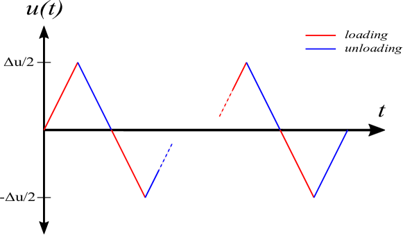
Figure 3: Loading conditions: piece-wise linear variation of the applied displacement under constant amplitude. Red segments correspond to loading stages.

The cyclic plasticity behaviour of the material is calibrated against the experiments by Nip et al. on hot-rolled carbon steels [5, 6]. The combined non-linear isotropic/kinematic hardening model described in Section 2.3.6 must be used to attain a good fit with the experimental data. The magnitudes of the isotropic ($Q_{\infty}$, $b$) and kinematic hardening parameters ($C$, $\gamma$) that provide the best agreement with the experiments are listed in Table 1, together with the initial yield stress $\sigma_{0}$ and the elastic properties (Young’s modulus $E$ and Poisson’s ratio $\nu$). Only one backstress is needed. Fig. 4 shows the agreement between the experimental data [5] and the present model over the first two cycles, for a representative strain amplitude of 1%.

Table 1: Material properties that provide the best fit to the experiments by Nip et al. [5, 6] on a hot-rolled carbon steel exhibiting combined non-linear isotropic/kinematic hardening behaviour.

E	$\nu$	$\sigma_{0}$	$Q_{\infty}$	$b$	$C$	$\gamma$
[MPa]	[-]	[MPa]	[MPa]	[-]	[MPa]	[-]
215,960	0.3	465	55	2.38	23,554	139

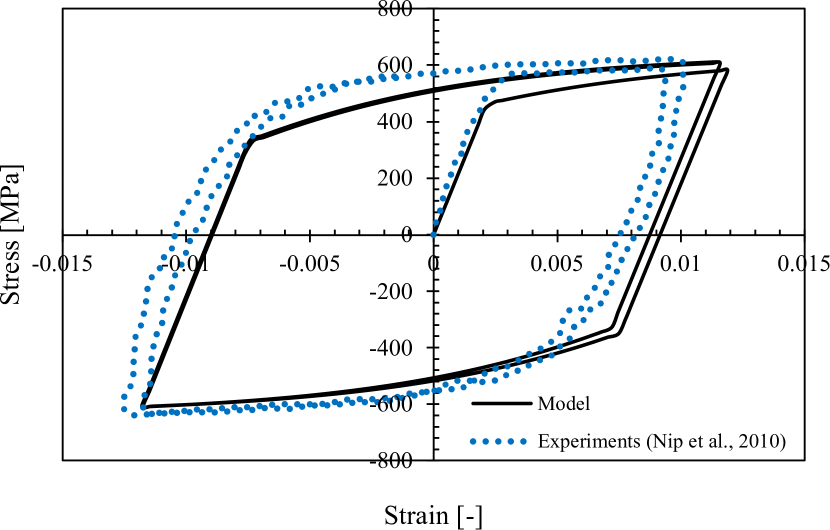
Figure 4: Non-linear kinematic/isotropic hardening material model calibration: model predictions for the first two cycles, compared with the experiments by Nip et al. [5].

The computational results obtained for selected values of the strain amplitude are reported in Fig. 5, using a log-log plot. Computations are performed using the AT2 model and the asymptotic fatigue degradation function. It is assumed that the sample has failed when the phase field reaches $\phi=0.9$. The magnitude of the material toughness is taken to be equal to $G_{c}=1000$ kJ/m² and we vary the phase field length scale $\ell$ to investigate the role of the strength and the fatigue threshold; recall (30) and (20), respectively. The numerical predictions are shown together with experimental data reported in the literature for carbon steels [67, 68, 69, 70] and with the measurements by Nip et al. [5, 6] on the hot-rolled carbon steel used for calibrating the non-linear combined isotropic/kinematic hardening model. Overall, a good agreement is attained with the experimental data but differences are observed at low and high strain amplitudes. The role of the various fatigue and fracture parameters of the model in changing predictions and improving the agreement with experiments is discussed below.

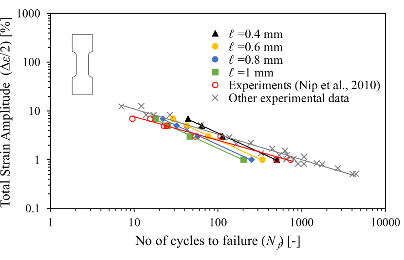
Figure 5: Uniaxial cyclic loading experiments: Total strain amplitude ($\Delta\varepsilon/2$) versus the number of cycles to failure ($N_{f}$). Numerical results for $G_{c}=1000$ kJ/m² and selected values of $\ell$ are compared against experimental data for carbon steels, as reported in the literature [67, 68, 69, 70, 5, 6].

A parametric study is conducted and the results are shown in Fig. 6. We keep the fatigue threshold $\vartheta_{T}$ fixed and investigate the influence on the predictions of the phase field length scale, the fracture energy and the fatigue degradation function. Consider first Fig. 6a, where the length scale is varied. It can be observed that a smaller length scale translates into a larger fatigue life for a given strain amplitude. This is due to the relation between $\ell$ and the strength in the AT2 model - see (30)b; the smaller the length scale, the larger the material strength. It can also be noted that the curves are closer to each other, relative to the results shown in Fig. 5. The higher sensitivity to $\ell$ observed in Fig. 5 is due to the relation between the phase field length scale and the fatigue threshold, see (20). A smaller value of $\ell$ leads to a larger $\vartheta_{T}$, while in Fig. 6a the magnitude of the threshold is fixed at $\vartheta_{T}=104.167$ MPa (corresponding to $\ell=0.4$ mm and $G_{c}=500$ kJ/m²) to isolate the influence of the phase field length scale. The influence of the material toughness is evaluated in Fig. 6b for $\ell=0.4$ mm. Four values of $G_{c}$ are considered: 100, 500, 800 and 1000 kJ/m². The results show significant sensitivity for low $G_{c}$ values, with the number of cycles to failure increasing with $G_{c}$, in agreement with expectations. However, one should note that the magnitude of the fracture energy does not typically influence the damage evolution law of cohesive zone models for fatigue [71, 72]. As for the case of varying $\ell$, changes in $G_{c}$ do not lead to noticeable variations in the slope of the curve. The role of the fatigue degradation function is explored in Fig. 6c for the choices $G_{c}=$ 1000 $\mathrm{kJ/m^{2}}$ and $\ell=$ 0.4 mm. Results are obtained for both asymptotic (16) and logarithmic (17) degradation functions, and the latter is assessed for selected values of $\kappa$ (0.3, 0.5, 0.8). Although differences are small for the values considered, it can be observed that the slope of the curve is sensitive to $\kappa$, with larger $\kappa$ values delivering fatigue responses that are more susceptible to changes in the strain amplitude. Thus, the use of a logarithmic degradation function provides additional flexibility, enabling a better match with the experimental results reported in Fig. 5. Finally, the role of the fatigue threshold is investigated in Fig. 6d. While $\vartheta_{T}$ can be assumed to depend only on the toughness and the phase field length scale $\ell$, as given in (20) and adopted in Figs. 5a-c, one can also adopt an independent value. The results obtained reveal a longer fatigue life for higher values of $\vartheta_{T}$, in agreement with expectations.

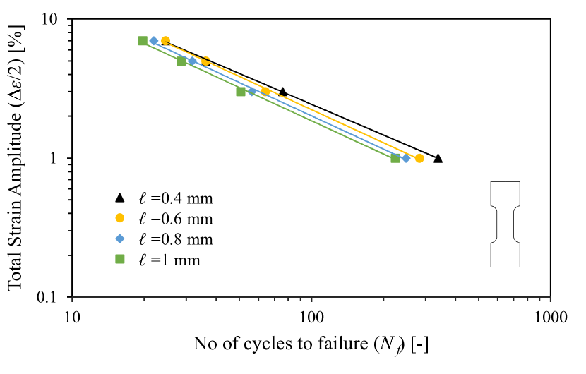
(a)

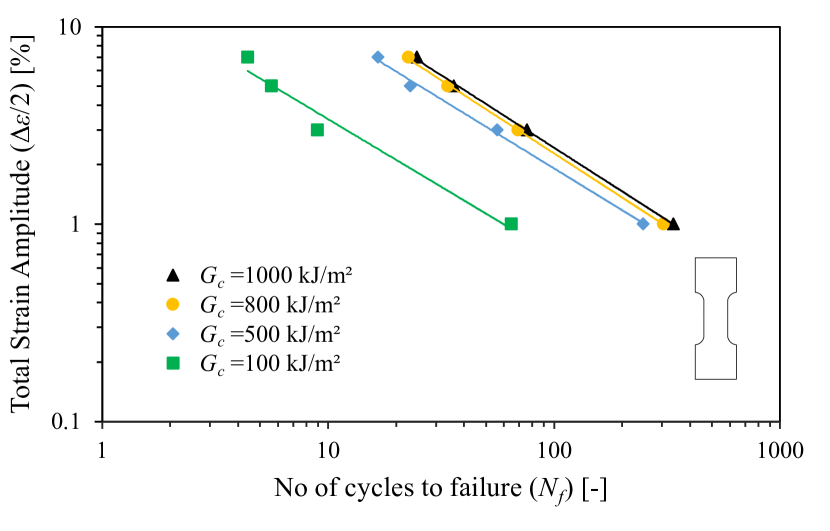
(b)

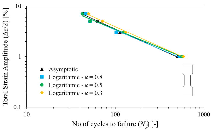
(c)

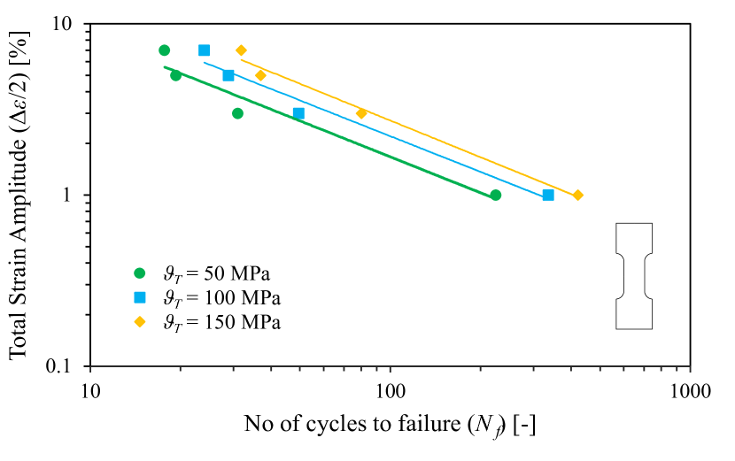
(d)

Figure 6: Uniaxial cyclic loading experiments: parametric study. Influence of (a) the length scale $\ell$, (b) the toughness $G_{c}$, (c) the fatigue degradation function, and (d) the fatigue threshold. In sub-figures (a)-(c), the fatigue threshold $\vartheta_{T}$ is held fixed, as given by (20), and in the results shown in (d) have been computed using the asymptotic degradation function.

4.2 Fatigue crack growth in a Compact-Tension specimen

The influence of the various phase field models and solution schemes presented above is investigated by modelling fatigue crack growth in a Compact Tension (CT) sample. The geometry and dimensions of the sample are shown in Fig. 7, together with the finite element mesh employed. A total of 19,521 4-node plane strain elements are used, with the characteristic element size in the crack propagation region being 5 times smaller than the phase field length scale. The specimen is subjected to symmetric quasi-static cyclic displacement at the pins, with an amplitude of 0.05 mm, a zero mean and a load ratio of $R=-1$. The nonlinear combined isotropic/kinematic hardening material model is used, with the material properties described in Table 1. The assumed values for the toughness and the phase field length scale are $G_{c}=2.7$ kJ/m² and $\ell=0.25$ mm, respectively.

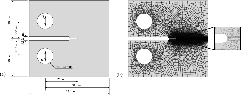
Figure 7: Fatigue crack growth in a CT specimen: (a) Geometry and boundary conditions and (b) finite element mesh.

We start by assessing the role of the constitutive choices for the phase field fracture description. As described in Section 2.3, three options are considered, corresponding to the so-called AT1, AT2, and PF-CZM models. In all three cases, the qualitative outcome is in good agreement; as shown in Fig. 8, the crack propagates in a stable manner along the expected mode I trajectory. However, noticeable differences are observed when evaluating the crack extension $\Delta a$ versus number of cycles $N$ curves, see Fig. 9.

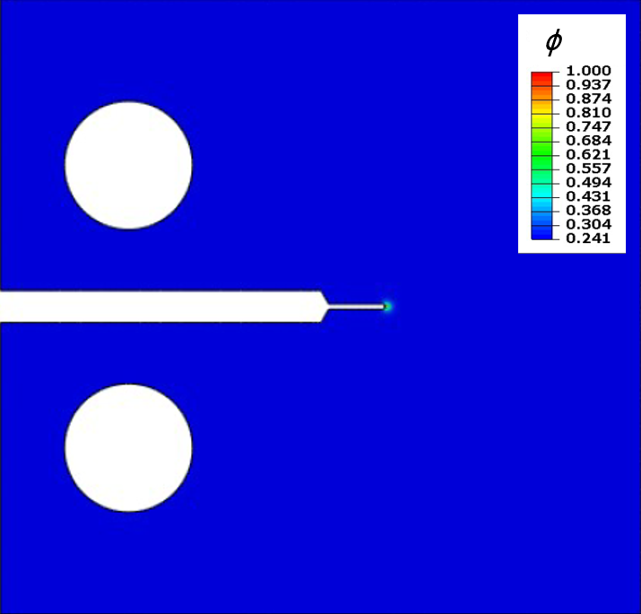
(a)

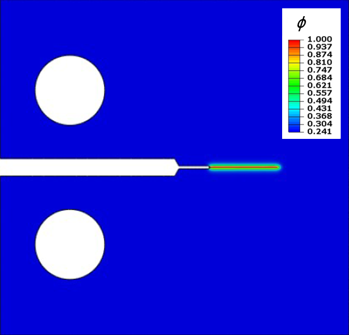
(b)

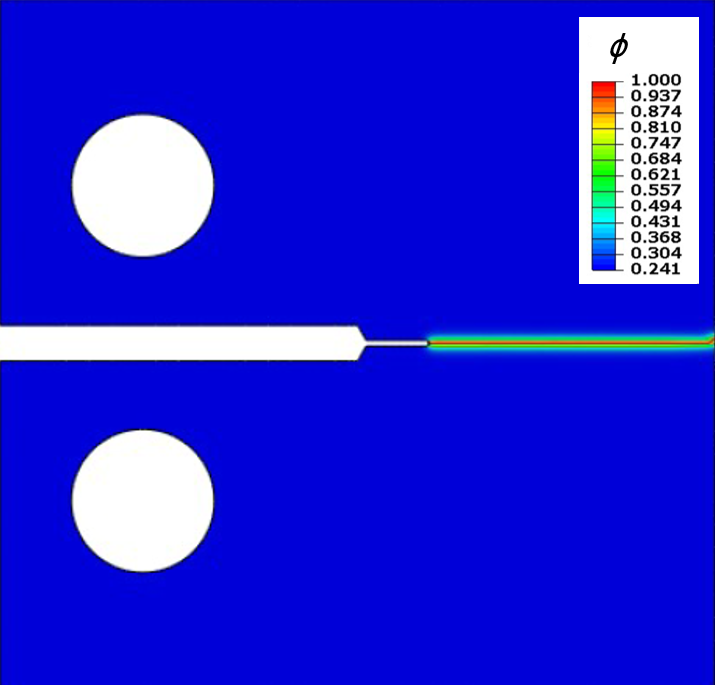
(c)

Figure 8: Fatigue crack growth in a CT specimen. Phase field contours at (a) 12 cycles, (b) 20 cycles and (c) 28 cycles. These representative results have been obtained with the AT1 model.

As shown in Fig. 9, fatigue crack growth curves are obtained for AT1, AT2, and PF-CZM models, with three values of the material strength ($\sigma_{c}$) being used in the PF-CZM case. Consider first the results predicted for AT1 and AT2 models; similar fatigue crack growth rates are predicted but the number of cycles to failure is higher for the AT1 case. This is attributed to the presence of a damage threshold, which is absent in the AT2 formulation, and to the higher material strength that results from considering Eq. (30) for the same $G_{c}$ and $\ell$ values. Specifically, Eq. (30) gives strength values of 935 MPa and 496 MPa for AT1 and AT2, respectively. As a result, the initiation of crack growth takes place later for the AT1 model, relative to the AT2 one. We emphasise that the degradation function is independent of $\ell$ (and thus of the strength) for the AT1 and AT2 models, see (26), and consequently fatigue crack growth rates are similar. However, the PF-CZM model predictions exhibit a different trend. The initiation of crack growth appears to be largely insensitive to the choice of $\sigma_{c}$ but fatigue crack growth rates differ, with smaller strength values being associated with larger fatigue lives. This is a result of the strength dependency of the phase field degradation function in the PF-CZM model - see (27); for a given $\phi$ magnitude, a greater stiffness degradation will be attained for a higher strength. It is also interesting to note that the predictions from the AT2 and PF-CZM models coincide when a strength of $\sigma_{c}=500$ MPa is used in the latter - versus $\sigma_{c}=496$ MPa for AT2, if estimated from (30). However, the AT1 result with an estimated strength of $\sigma_{c}=935$ MPa lies between the PF-CZM predictions for $\sigma_{c}=500$ and $\sigma_{c}=200$ MPa. There is a need to determine the most physically sound relation between $G_{c}$, $\sigma_{c}$ and $\ell$, given that the length scale governs the size of the fracture process zone and thus cannot be purely seen as a numerical parameter.

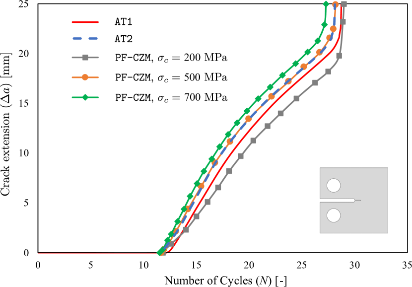
Figure 9: Fatigue crack growth in a CT specimen: influence of the phase field formulation. Crack extension $\Delta a$ versus number of cycles $N$, as predicted by the AT1, AT2, and PF-CZM models.

The influence of the solution scheme is examined next. Specifically, we compare the performance of the monolithic quasi-Newton algorithm presented in Section 3.3 with a single-pass, alternative minimisation staggered scheme.. Monolithic approaches are unconditionally stable, implying that results are independent of the number of load increments used. This is not the case for staggered approaches, and consequently we obtain results for four load stepping choices: 16, 40, 200 and 400 increments per cycle. As shown in Fig. 10, the staggered solution converges slowly towards the monolithic one. Even when using 400 load increments per cycle, the fatigue crack growth curve obtained does not match the monolithic result (obtained with 16 increments per cycle). Differences become very significant when reducing the number of load increments. Furthermore, convergence problems are observed for the simulations with a low number of increments (16 and 40 increments per cycle), with calculations stopping after 17 cycles. Thus, these results show that monolithic quasi-Newton schemes are more robust and significantly more efficient than widely used staggered schemes, which can require prohibitive computation times for accurate cycle-by-cycle predictions of high cycle fatigue.

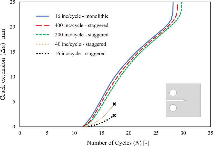
Figure 10: Fatigue crack growth in a CT specimen: influence of the solution scheme. Crack extension $\Delta a$ versus number of cycles $N$ as predicted with a staggered and a monolithic quasi-Newton scheme. The phase field AT2 model has been used.

4.3 Failure of an asymmetrically-notched plate

We proceed to investigate the interplay between cyclic hardening and damage by simulating the fatigue failure of an asymmetrically-notched plate. The geometry, boundary conditions and dimensions (in mm) are shown in Fig. 11a. The specimen is discretised with a total of 95,854 linear quadrilateral plane strain elements. As shown in Fig. 11b, the finite element mesh is refined along the crack propagation path, with the characteristic element size being at least four times smaller than the phase field length scale. The specimen is subjected to a symmetric quasi-static cyclic displacement of amplitude 0.5 mm, with zero mean and a load ratio of $R=-1$. The fracture behaviour is characterised by the AT2 model, with properties $G_{c}=8000$ kJ/m² and $\ell=0.04$ mm.

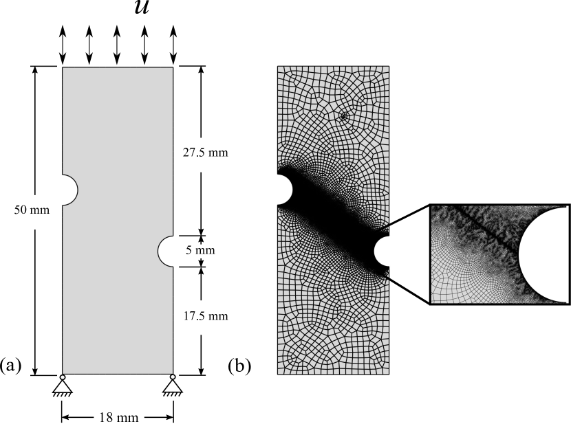
Figure 11: Asymmetrically-notched specimen subjected to cyclic axial load: (a) Geometry and boundary conditions and (b) finite element mesh.

One of the aims of this case study is to assess the role of kinematic and isotropic hardening effects. Thus, the material constitutive behavior is given by the non-linear combined isotropic/kinematic hardening model described in Section 2.3, with the material properties listed in Table 1, but calculations are also conducted for the cases of purely isotropic hardening ($C=\gamma=0$) and purely kinematic hardening ($\sigma_{Y}=\sigma_{0}$). The results obtained for the three material models under consideration are shown in Fig. 12, in terms of both the force versus displacement (Fig. 12a) and force versus number of cycles (Fig. 12b) responses. The results shown in Fig. 12a show how the values of maximum force attained change more significantly with the number of cycles when kinematic hardening effects are accounted for, as a result of the Bauschinger effect. Substantial differences are observed over the first cycles, highlighting the importance of properly characterising the cyclic behaviour of the solid. However, the differences between the three models are reduced as damage starts to govern the material response. As shown in Fig. 12b, the higher strain energy levels attained with the combined and non-linear kinematic hardening models result in a faster damage rate, while damage is underestimated for the purely isotropic hardening case. This is intrinsic to our choice of an elastic-plastic driving force; see Eqs. (8)-(9).

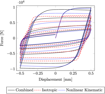
(a)

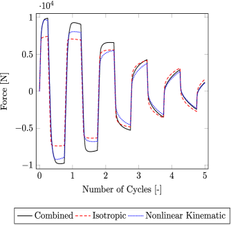
(b)

Figure 12: Asymmetrically-notched specimen subjected to cyclic axial load: (a) Force versus displacement response, and (b) Force versus number of cycles response.

4.4 Fatigue crack growth in a pipe-to-pipe connection

Finally, we conclude our numerical experiments by demonstrating the capabilities of the framework presented for predicting large scale fatigue failures in solids exhibiting combined non-linear isotropic/kinematic hardening. To this end, fatigue crack nucleation and growth is simulated in a pipe-to-pipe connection composed of two orthogonal circular pipes - see Fig. 13. The horizontal pipe has an outer diameter of 100 mm and thickness of 8 mm, while the vertical pipe has on outer diameter of 80 mm and thickness of 6 mm. A quarter of the geometry is modelled due to symmetry. The domain is discretised with 10-node tetrahedral solid elements, employing approximately 200,000 degrees-of-freedom. As shown in Fig. 13b, the mesh is refined at the intersection between the two pipes, where fatigue damage is expected to take place. The vertical pipe is subjected to symmetric quasi-static cyclic displacement of amplitude of 0.5 mm with a load ratio of $R=-1$. The horizontal pipeline is clamped on one end. The AT-2 phase field damage model is used along with the nonlinear combined isotropic/kinematic hardening constitutive description. The cyclic deformation is characterised by the material properties listed in Table 1. The assumed values of $G_{c}$ and $\ell$ are $100$ $\mathrm{kJ/m^{2}}$ and 2.5 mm, respectively.

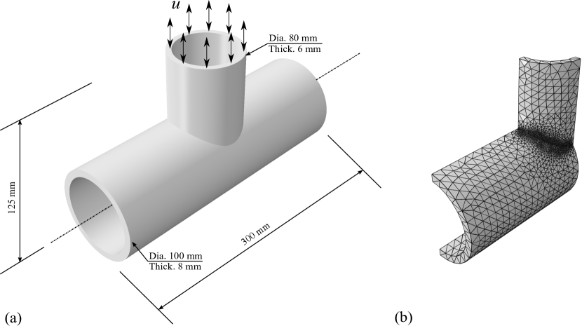
Figure 13: 3D pipe-to-pipe connection subjected to cyclic axial load: (a) Geometry and (b) finite element mesh.

The process of crack nucleation and growth is depicted in Fig. 14. Four stages of the cracking process are shown, from the initiation of damage to the complete rupture of the pipe-to-pipe connection. We emphasise that no initial defects are introduced in the model.

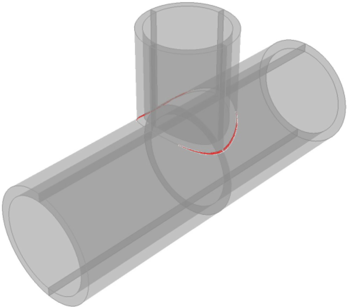
(a)

(b)

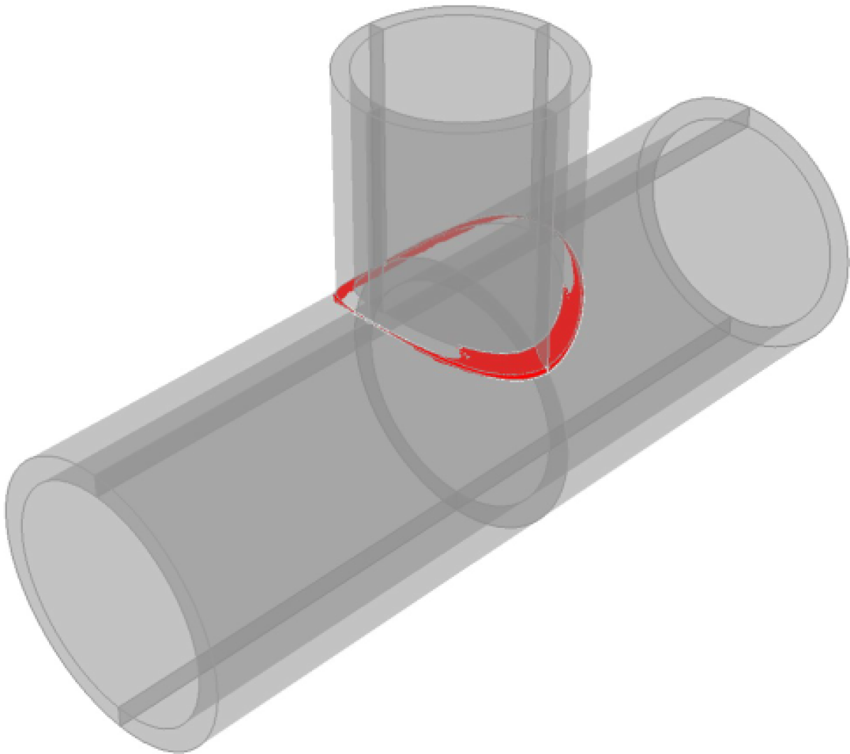
(c)

(d)

Figure 14: 3D pipe-to-pipe connection subjected to cyclic axial load. Crack surface ($\phi>0.9$) after: (a) 5 cycles, (b) 8 cycles, (c) 10 cycles and (d) 12 cycles.

Finally, Fig. 15 shows a detailed view of the extent of the crack at the time of complete failure. The results show that the model can naturally predict crack growth due to fatigue damage under cyclic loading in three-dimensional settings for arbitrary geometries and dimensions.

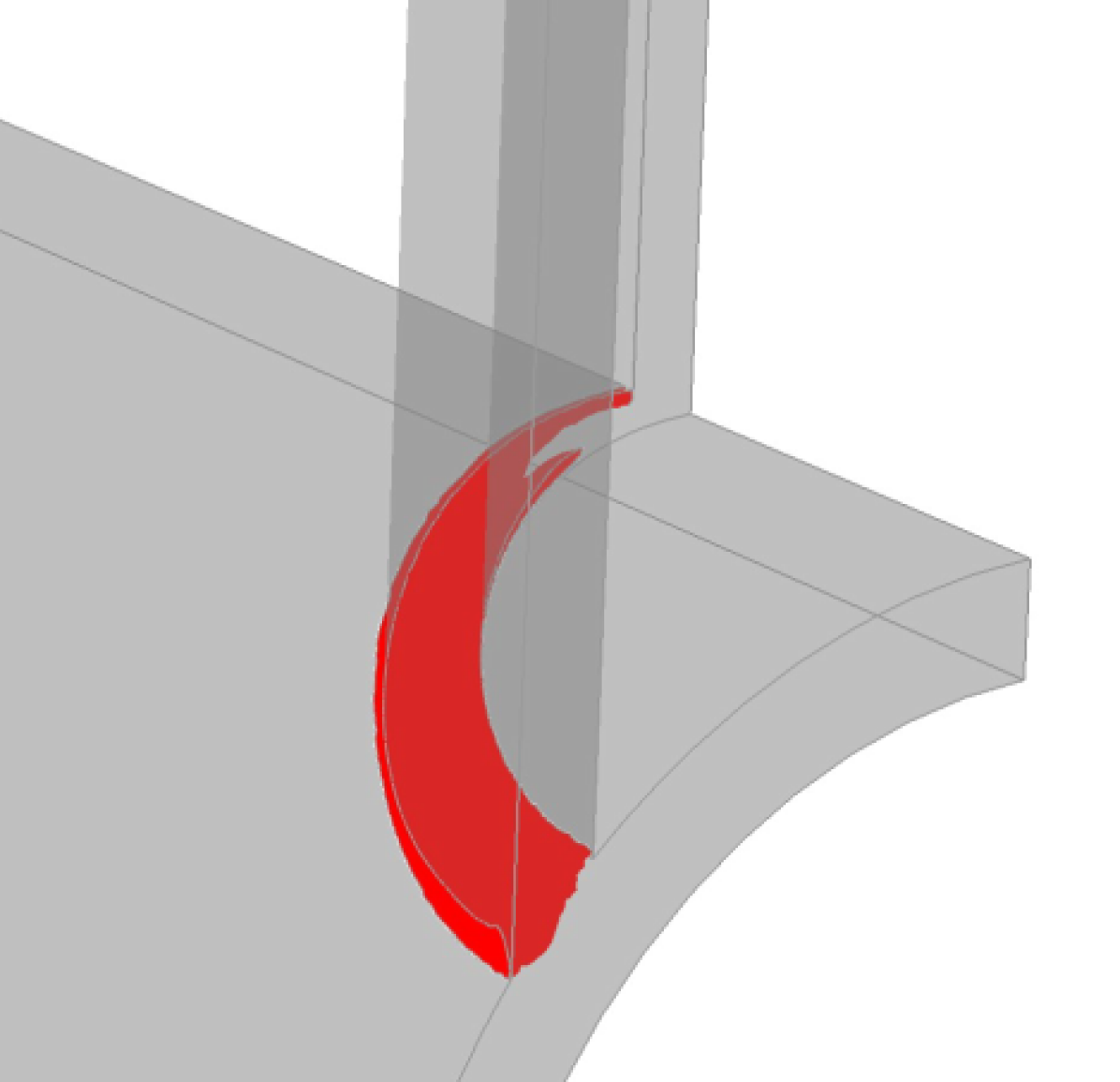
Figure 15: 3D pipe-to-pipe connection subjected to cyclic axial load. Detailed plot of the crack surface ($\phi>0.9$) at 12 cycles.

5 Conclusions

We have presented a generalised formulation for modelling fatigue crack growth in elastic-plastic solids. The initiation and growth of cracks is captured by means of a unified phase field formulation, that incorporates as special cases the so-called AT1, AT2 and PF-CZM models. Two classes of fatigue degradation functions (asymptotic and logarithmic) are defined to capture fatigue damage, which is driven by both elastic and plastic mechanical fields. The cyclic deformation of the solid is characterised by a combined, non-linear kinematic/isotropic hardening model that can be used to model the cyclic response of a general class of elastic-plastic materials. The theoretical framework presented is numerically implemented using the finite element method and the resulting system of equations is solved in a monolithic manner, by exploiting a quasi-Newton algorithm. Several 2D and 3D case studies are modelled to gain insight into the role of the phase field formulation and the interplay between damage and cyclic hardening effects. Key findings include:

(i) The model provides a good agreement with experimental data on carbon steels. However, the additional flexibility provided by the logarithmic degradation function is needed to capture the appropriate damage scaling. This comes at the cost of defining one additional parameter.

(ii) Fatigue crack growth predictions differ between those obtained with phase field models based on the Ambrosio-Tortorelli functional (AT1, AT2) and those inspired in cohesive laws, such as the PF-CZM. In the PF-CZM, higher fatigue crack growth rates are predicted with increasing material strength $\sigma_{c}$, due to the $\sigma_{c}$-dependency of the fracture degradation function.

(iii) The use of quasi-Newton monolithic solution schemes delivers a more robust and efficient performance than widely-used staggered approaches. The staggered scheme requires over 25 times more load increments to match the monolithic result. The implications are important, given the inherent cost of cycle-by-cycle predictions.

(iv) For a crack driving force that includes both elastic and plastic contributions, neglecting kinematic hardening phenomena such as the Bauschinger effect is non-conservative, and can lead to a significant underestimation of damage.

The case studies addressed show how the modelling framework presented can be used to efficiently predict fatigue crack initiation and growth in arbitrary dimensions and geometries, and for solids exhibiting complex cyclic deformation responses. The finite element code developed can be downloaded from www.empaneda.com/codes.

6 Acknowledgments

E. Martínez-Pañeda acknowledges financial support from the EPSRC (grant EP/V009680/1) and from the Royal Commission for the 1851 Exhibition (RF496/2018). Z. Khalil acknowledges the MSc Scholarship support provided by the Department of Civil and Environmental Engineering at Imperial College London.

References

- [1] S. Suresh, Fatigue of Materials, Cambridge University Press, Cambridge, UK, 1998.
- [2] A. Wöhler, Über die Festigkeitsversuche mit Eisen und Stahl, Zeitschrift für Bauwesen 20 (1870) 73–106.
- [3] J. L. Coffin, A study of the effects of cyclic thermal stresses on a ductile metal, Transactions of the ASME 76 (1954) 931–950.
- [4] S. S. Manson, Behavior of materials under conditions of thermal stress, Tech. rep., National Advisory Committee for Aeronautics (1954).
- [5] K. H. Nip, L. Gardner, C. M. Davies, A. Y. Elghazouli, Extremely low cycle fatigue tests on structural carbon steel and stainless steel, Journal of Constructional Steel Research 66 (1) (2010) 96–110.
- [6] K. H. Nip, L. Gardner, A. Y. Elghazouli, Cyclic testing and numerical modelling of carbon steel and stainless steel tubular bracing members, Engineering Structures 32 (2) (2010) 424–441.
- [7] A. A. Griffith, The Phenomena of Rupture and Flow in Solids, Philosophical Transactions A, 221 (1920) 163–198.
- [8] G. R. Irwin, Onset of Fast Crack Propagation in High Strength Steel and Aluminum Alloys, in: Sagamore Research Conference Proceedings Vol. 2, 1956, pp. 289–305.
- [9] G. A. Francfort, J.-J. Marigo, Revisiting brittle fracture as an energy minimization problem, Journal of the Mechanics and Physics of Solids 46 (8) (1998) 1319–1342.
- [10] D. Mumford, J. Shah, Optimal approximations by piecewise smooth functions and associated variational problems, Communications on Pure and Applied Mathematics 42 (5) (1989) 577–685.
- [11] B. Bourdin, G. A. Francfort, J.-J. Marigo, Numerical experiments in revisited brittle fracture, Journal of the Mechanics and Physics of Solids 48 (4) (2000) 797–826.
- [12] B. Bourdin, G. A. Francfort, J. J. Marigo, The variational approach to fracture, Springer Netherlands, 2008.
- [13] C. Miehe, F. Welshinger, M. Hofacker, Thermodynamically consistent phase-field models of fracture: Variational principles and multi-field FE implementations, International Journal for Numerical Methods in Engineering 83 (2010) 1273–1311.
- [14] C. Miehe, M. Hofacker, F. Welschinger, A phase field model for rate-independent crack propagation: Robust algorithmic implementation based on operator splits, Computer Methods in Applied Mechanics and Engineering 199 (45-48) (2010) 2765–2778.
- [15] M. J. Borden, C. V. Verhoosel, M. A. Scott, T. J. R. Hughes, C. M. Landis, A phase-field description of dynamic brittle fracture, Computer Methods in Applied Mechanics and Engineering 217-220 (2012) 77–95.
- [16] R. J. Geelen, Y. Liu, T. Hu, M. R. Tupek, J. E. Dolbow, A phase-field formulation for dynamic cohesive fracture, Computer Methods in Applied Mechanics and Engineering 348 (2019) 680–711.
- [17] G. Molnár, A. Gravouil, R. Seghir, J. Réthoré, An open-source Abaqus implementation of the phase-field method to study the effect of plasticity on the instantaneous fracture toughness in dynamic crack propagation, Computer Methods in Applied Mechanics and Engineering 365 (2020) 113004.
- [18] R. Alessi, F. Freddi, Failure and complex crack patterns in hybrid laminates: A phase-field approach, Composites Part B: Engineering 179 (2019) 107256.
- [19] A. Quintanas-Corominas, A. Turon, J. Reinoso, E. Casoni, M. Paggi, J. A. Mayugo, A phase field approach enhanced with a cohesive zone model for modeling delamination induced by matrix cracking, Computer Methods in Applied Mechanics and Engineering 358 (2020) 112618.
- [20] T. K. Mandal, V. P. Nguyen, J.-Y. Wu, A length scale insensitive anisotropic phase field fracture model for hyperelastic composites, International Journal of Mechanical Sciences 188 (2020) 105941.
- [21] W. Tan, E. Martínez-Pañeda, Phase field predictions of microscopic fracture and R-curve behaviour of fibre-reinforced composites, Composites Science and Technology 202 (2021) 108539.
- [22] M. Ambati, T. Gerasimov, L. De Lorenzis, Phase-field modeling of ductile fracture, Computational Mechanics 55 (5) (2015) 1017–1040.
- [23] M. J. Borden, T. J. R. Hughes, C. M. Landis, A. Anvari, I. J. Lee, A phase-field formulation for fracture in ductile materials: Finite deformation balance law derivation, plastic degradation, and stress triaxiality effects, Computer Methods in Applied Mechanics and Engineering 312 (2016) 130–166.
- [24] M. Isfandbod, E. Martínez-Pañeda, A mechanism-based multi-trap phase field model for hydrogen assisted fracture, International Journal of Plasticity 144 (2021) 103044.
- [25] E. Martínez-Pañeda, A. Golahmar, C. F. Niordson, A phase field formulation for hydrogen assisted cracking, Computer Methods in Applied Mechanics and Engineering 342 (2018) 742–761.
- [26] F. P. Duda, A. Ciarbonetti, S. Toro, A. E. Huespe, A phase-field model for solute-assisted brittle fracture in elastic-plastic solids, International Journal of Plasticity 102 (2018) 16–40.
- [27] J.-Y. Wu, T. K. Mandal, V. P. Nguyen, A phase-field regularized cohesive zone model for hydrogen assisted cracking, Computer Methods in Applied Mechanics and Engineering 358 (2020) 112614.
- [28] P. K. Kristensen, C. F. Niordson, E. Martínez-Pañeda, Applications of phase field fracture in modelling hydrogen assisted failures, Theoretical and Applied Fracture Mechanics 110 (2020) 102837.
- [29] Hirshikesh, S. Natarajan, R. K. Annabattula, E. Martínez-Pañeda, Phase field modelling of crack propagation in functionally graded materials, Composites Part B: Engineering 169 (2019) 239–248.
- [30] P. K. A. V. Kumar, A. Dean, J. Reinoso, P. Lenarda, M. Paggi, Phase field modeling of fracture in Functionally Graded Materials: G -convergence and mechanical insight on the effect of grading, Thin-Walled Structures 159 (2021) 107234.
- [31] J.-Y. Wu, V. P. Nguyen, C. T. Nguyen, D. Sutula, S. Sinaie, S. Bordas, Phase-field modelling of fracture, Advances in Applied Mechanics 53 (2020) 1–183.
- [32] P. K. Kristensen, C. F. Niordson, E. Martínez-Pañeda, An assessment of phase field fracture: crack initiation and growth, Philosophical Transactions of the Royal Society A: Mathematical, Physical and Engineering Sciences 379 (2021) 20210021.
- [33] R. Alessi, S. Vidoli, L. De Lorenzis, A phenomenological approach to fatigue with a variational phase-field model: The one-dimensional case, Engineering Fracture Mechanics 190 (2018) 53–73.
- [34] Y. S. Lo, M. J. Borden, K. Ravi-Chandar, C. M. Landis, A phase-field model for fatigue crack growth, Journal of the Mechanics and Physics of Solids 132 (2019) 103684.
- [35] P. Carrara, M. Ambati, R. Alessi, L. De Lorenzis, A framework to model the fatigue behavior of brittle materials based on a variational phase-field approach, Computer Methods in Applied Mechanics and Engineering 361 (2020) 112731.
- [36] M. Simoes, E. Martínez-Pañeda, Phase field modelling of fracture and fatigue in Shape Memory Alloys, Computer Methods in Applied Mechanics and Engineering 373 (2021) 113504.
- [37] M. M. Hasan, T. Baxevanis, A phase-field model for low-cycle fatigue of brittle materials, International Journal of Fatigue 150 (2021) 106297.
- [38] A. Golahmar, P. K. Kristensen, C. F. Niordson, E. Martínez-Pañeda, A phase field model for hydrogen-assisted fatigue, International Journal of Fatigue 154 (2022) 106521.
- [39] M. Seiler, T. Linse, P. Hantschke, M. Kästner, An efficient phase-field model for fatigue fracture in ductile materials, Engineering Fracture Mechanics 224 (2020) 106807.
- [40] G. A. Haveroth, M. G. Vale, M. L. Bittencourt, J. L. Boldrini, A non-isothermal thermodynamically consistent phase field model for damage, fracture and fatigue evolutions in elasto-plastic materials, Computer Methods in Applied Mechanics and Engineering 364 (2020) 112962.
- [41] J. Ulloa, J. Wambacq, R. Alessi, G. Degrande, S. François, Phase-field modeling of fatigue coupled to cyclic plasticity in an energetic formulation, Computer Methods in Applied Mechanics and Engineering 373 (2021) 113473.
- [42] N. Provatas, K. Elder, Phase-Field Methods in Materials Science and Engineering, John Wiley & Sons, Weinheim, Germany, 2011.
- [43] C. Cui, R. Ma, E. Martínez-Pañeda, A phase field formulation for dissolution-driven stress corrosion cracking, Journal of the Mechanics and Physics of Solids 147 (2021) 104254.
- [44] M. E. Gurtin, E. Fried, L. Anand, The Mechanics and Thermodynamics of continua, Cambridge University Press, Cambridge, UK, 2010.
- [45] F. P. Duda, A. Ciarbonetti, P. J. Sánchez, A. E. Huespe, A phase-field/gradient damage model for brittle fracture in elastic-plastic solids, International Journal of Plasticity 65 (2015) 269–296.
- [46] S. Narayan, L. Anand, A gradient-damage theory for fracture of quasi-brittle materials, Journal of the Mechanics and Physics of Solids 129 (2019) 119–146.
- [47] R. Alessi, M. Ambati, T. Gerasimov, S. Vidoli, L. De Lorenzis, Comparison of Phase-Field Models of Fracture Coupled with Plasticity, in: M. C. E. Oñate, D. Peric, E. de Souza- Neto (Ed.), Advances in Computational Plasticity, Springer Nature, 2018, pp. 1–21.
- [48] H. Amor, J. J. Marigo, C. Maurini, Regularized formulation of the variational brittle fracture with unilateral contact: Numerical experiments, Journal of the Mechanics and Physics of Solids 57 (8) (2009) 1209–1229.
- [49] C. Miehe, F. Aldakheel, A. Raina, Phase field modeling of ductile fracture at finite strains: A variational gradient-extended plasticity-damage theory, International Journal of Plasticity 84 (2016) 1–32.
- [50] S. S. Shishvan, S. Assadpour-asl, E. Martínez-Pañeda, A mechanism-based gradient damage model for metallic fracture, Engineering Fracture Mechanics 255 (2021) 107927.
- [51] P. K. Kristensen, C. F. Niordson, E. Martínez-Pañeda, A phase field model for elastic-gradient-plastic solids undergoing hydrogen embrittlement, Journal of the Mechanics and Physics of Solids 143 (2020) 104093.
- [52] J. Bleyer, R. Alessi, Phase-field modeling of anisotropic brittle fracture including several damage mechanisms, Computer Methods in Applied Mechanics and Engineering 336 (2018) 213–236.
- [53] Y. Navidtehrani, C. Betegón, E. Martínez-Pañeda, A Unified Abaqus Implementation of the Phase Field Fracture Method Using Only a User Material Subroutine, Materials 14 (8) (2021) 1913.
- [54] L. Ambrosio, V. M. Tortorelli, Approximation of functionals depending on jumps by elliptic functionals via gamma-convergence, Communications on Pure and Applied Mathematics 43 (1991) 999–1036.
- [55] K. Pham, H. Amor, J. J. Marigo, C. Maurini, Gradient damage models and their use to approximate brittle fracture, International Journal of Damage Mechanics 20 (4) (2011) 618–652.
- [56] J.-Y. Wu, A unified phase-field theory for the mechanics of damage and quasi-brittle failure, Journal of the Mechanics and Physics of Solids 103 (2017) 72–99.
- [57] J.-Y. Wu, V. P. Nguyen, A length scale insensitive phase-field damage model for brittle fracture, Journal of the Mechanics and Physics of Solids 119 (2018) 20–42.
- [58] J. Lemaitre, J.-L. Chaboche, Mechanics of solid materials, Vol. 19, Cambridge University Press, New York, 1990.
- [59] H. Ziegler, A modification of Prager’s hardening rule, Quarterly of Applied Mathematics 17 (1) (1959) 55–65.
- [60] M. Ambati, T. Gerasimov, L. De Lorenzis, A review on phase-field models of brittle fracture and a new fast hybrid formulation, Computational Mechanics 55 (2015) 383–405.
- [61] J.-Y. Wu, Y. Huang, V. P. Nguyen, On the BFGS monolithic algorithm for the unified phase field damage theory, Computer Methods in Applied Mechanics and Engineering 360 (2020) 112704.
- [62] P. K. Kristensen, E. Martínez-Pañeda, Phase field fracture modelling using quasi-Newton methods and a new adaptive step scheme, Theoretical and Applied Fracture Mechanics 107 (2020) 102446.
- [63] D. H. Li, M. Fukushima, A modified BFGS method and its global convergence in nonconvex minimization, Journal of Computational and Applied Mathematics 129 (1-2) (2001) 15–35.
- [64] A. S. Lewis, M. L. Overton, Nonsmooth optimization via quasi-Newton methods, Mathematical Programming 141 (1-2) (2013) 135–163.
- [65] M. Geradin, S. Idelsohn, M. Hogge, Computational strategies for the solution of large nonlinear problems via quasi-newton methods, Computers and Structures 13 (1-3) (1981) 73–81.
- [66] H. Matthies, G. Strang, The solution of nonlinear finite element equations, International Journal for Numerical Methods in Engineering 14 (1979) 1613–1626.
- [67] R. W. Smith, M. H. Hirschberg, S. S. Manson, Fatigue behavior of materials under strain cycling in low and intermediate life range, Tech. rep., NASA (1963).
- [68] D. Lefebvre, F. Ellyin, Cyclic response and inelastic strain energy in low cycle fatigue, International Journal of Fatigue 6 (1) (1984) 9–15.
- [69] Y. Gong, M. Norton, Cyclic Response and Fatigue of Steels Subjected to Strain Control with Non-Zero Means, Journal of Testing and Evaluation 27 (1) (1999) 15–30.
- [70] X. Yang, Low cycle fatigue and cyclic stress ratcheting failure behavior of carbon steel 45 under uniaxial cyclic loading, International Journal of Fatigue 27 (9) (2005) 1124–1132.
- [71] K. Roe, T. Siegmund, An irreversible cohesive zone model for interface fatigue crack growth simulation, Engineering Fracture Mechanics 70 (2) (2003) 209–232.
- [72] S. del Busto, C. Betegón, E. Martínez-Pañeda, A cohesive zone framework for environmentally assisted fatigue, Engineering Fracture Mechanics 185 (2017) 210–226.
- [73] E. Storvik, J. W. Both, J. M. Sargado, J. M. Nordbotten, F. A. Radu, An accelerated staggered scheme for variational phase-field models of brittle fracture, Computer Methods in Applied Mechanics and Engineering 381 (2021) 113822.