Periods of the Long-Term Variability of the Blazar 0716+714 and
Their Inter-Correlations in a Helical Jet Model

Abstract

Various quasi-periods for the long-term variability of the radio emission, optical emission, and structural position angle of the inner part of the parsec-scale jet in the blazar 0716+714 have been detected. The relationships between these quasi-periods are interpreted assuming that the variability arises due to helical structure of the jet, which is preserved from regions near the jet base to at least 1 milliarcsecond from the core observed in radio interferometric observations. The radiating jet components should display radial motions with Lorentz factors of $\approx 3$, and decelerate with distance from the jet base. The best agreement with the data is given in the case of non-radial motions of these components with a constant physical speed. It is also shown that the helical shape of the jet strongly influences correlations both between fluxes observed in different spectral ranges and between the flux and position angle of the inner part of the parsec-scale jet.

Astronomy Reports, Volume 62, Issue 10, pp.654-663, 2018, DOI: 10.1134/S1063772918100037

1 Introduction

Blazars are a class of Active Galactic Nuclei (AGN) whose relativistic parsec-scale jets are oriented close to the line of sight. Therefore, the flux density emitted by the jet is enhanced by relativistic effects in the observer’s frame, so that it dominates the emission of other parts of the AGN. This may be able to explain the fact that no lines are observed in the spectrum of the blazar 0716+714. Indirect estimates of its redshift have yielded $z\approx 0.31$ (Bychkova et al., 2006; Nilsson et al., 2008), $0.2315<z<0.3407$ (Danforth et al., 2013), and $z\geq 0.52$ (Sbarufatti et al., 2005). This object is variable over the entire electromagnetic spectrum, on both short and long time scales (see, e.g., Wagner et al., 1996; Raiteri et al., 2003; Wu et al., 2007; Poon et al., 2009; Gorshkov et al., 2011; Volvach et al., 2012; Rani et al., 2013; Liao et al., 2014; Bychkova et al., 2015).

0716+714 has also been observed with Very Long Baseline Interferometry (VLBI) in the framework of a 2 cm survey using the Very Long Baseline Array (VLBA), and monitored as part of the MOJAVE project (see, e.g., Bach et al., 2005; Lister et al., 2013; Pushkarev et al., 2017). The bright compact VLBI core visible in these maps is the region of the jet where the medium becomes optical thin to radiation at the given wavelength. For more than 150 sources (including 0716+714), the position of the VLBI core has been found to shift closer to the jet base with increasing frequency (Pushkarev et al., 2012), interpreted as an effect of synchrotron self-absorption in the jet (Marcaide & Shapiro, 1984; Lobanov, 1998; Kovalev et al., 2008). That is, the magnetic-field strength and density of the radiating particles decrease with distance from the jet base, so that the medium becomes optically thin to radiation at increasingly lower frequencies. Synchrotron self-absorption could also be responsible for the observed delays between flares observed at different radio frequencies on single dishes (see, e.g., Kudryavtseva et al., 2011; Agarwal et al., 2017). Without interpretation by synchrotron selfabsorption a number of authors have found time delays between variability at different radio frequencies and in different spectral ranges.

For example, Raiteri et al. (2003) found that the delay between the variability of 0716+714 at 22$-$23 GHz and 15 GHz is 6$-$9 days, between 22$-$23 and 8 GHz is 22$\pm$2${}^{\text{d}}$, and between 15 and 5 GHz is 53$\pm$2${}^{\text{d}}$. No reliable correlation between the optical and 15 GHz fluxes has been found. However, Rani et al. (2013) found a correlation between the V and 230 GHz fluxes with a time delay of $\approx 65^{\text{d}}$. The delay between the optical and gamma-ray ranges is $\approx 1.4^{\text{d}}$ (Larionov et al., 2013). The millimeter wave length variability lags the gamma-ray variability by $82\pm 32^{\text{d}}$ (Rani et al., 2014). Wu et al. (2007) and Poon et al. (2009) attempted to determine the delays between the variability of 0716+714 in different optical bands. If there are such delays, they are less than the time resolution of those observations.

Thus, the flux variability at low frequencies is delayed compared to the variability at higher frequencies. Analyses of long-term series of observations reveal different quasi-periods for the long-term optical ($\approx 3.3$ yrs (Raiteri et al., 2003)) and radio (5.5$-$6 yrs (Raiteri et al., 2003; Bychkova et al., 2015; Liu et al., 2012) variability, and also for variations in the position angle of the inner jet PA${}_{\text{in}}$ ($\approx 11$ yrs Lister et al. (2013)).

The variations of PA${}_{\text{in}}$ can be explained in a natural way if the jet has a helical shape (Bach et al., 2005; Lister et al., 2013), which also often provides the simplest interpretation of a variety of observed properties of AGNs. For example, in the case of 0716+714, variations in the spectral energy distribution (Ostorero et al., 2001) and the kinematics of features in the parsec-scale jet (Butuzova, 2018) have both been explained in this way. The helical jet shape also gives rise to periodic variations in the viewing angle of the radiating regions, leading to corresponding variations of the Doppler factor, which should be manifest as longterm periodicity of the flux variations. The differences in the long-term periods for the radio variability, optical variability, and PA${}_{\text{in}}$ variations can be explained by either an overall deceleration of the speed of the jet or non-radial motions of the radiating regions in the jet. The latter is most probable for 0716+714 (see Section 2). Section 3 presents interpretations of the following results. The first is the opposite results obtained in searches for correlations between the radio and optical flux variations using the same statistical method (Raiteri et al., 2003; Rani et al., 2013) The second is the fact that time intervals when there is a strong positive correlation between PA${}_{\text{in}}$ and the gamma-ray flux alternate with intervals in which there is a strong negative correlation between these quantities (Rani et al., 2014). A discussion of the obtained results and our conclusions are presented in Section 4.

2 Relationship between the long-term variability periods for various observed quantities

Analysis of many-year radio and optical light curves of the blazar 0716+714 indicate the presence of quasi-periods in the long-term variability. Optical data for 1994$-$2001 indicated a period of about 3.3 yrs (Raiteri et al., 2003). This period was never confirmed, possibly because other studies considered data obtained over shorter time intervals. For example, Rani et al. (2013) did not detect any reliable periods for the long-term variability in their analysis of data for 2007$-$2010. It is difficult to detect long-term periodicity in the optical due to the superposition of short-term flares on the longer-term trend. In the radio, where the flare component is weaker, variability periods of 5.6$-$6 yrs at 14.5 and 15 GHz for 1978$-$2001 (Raiteri et al., 2003), 5.5$-$6 yrs at 22 GHz for 1992.7$-$2001.2 (Bach et al., 2005), and $5.8\pm 0.4$ yrs at 15 GHz for data after 2001 (Liu et al., 2012) have been found.

Data from more than 30 years of observations carried out on telescopes of the Crimean Astrophysical Observatory (CrAO), the Metsahovi Radio Observatory, and the University of Michigan Radio Astronomy Observatory at frequencies from 4.8 to 36.8 GHz also indicate the presence of a period of $\approx 8$ yrs, together with shorter periods (Bychkova et al., 2015). Quasi-periodicity is also present in the variations of the position angle of the inner parsec-scale jet of 0716+714. Analysis of data for 26 epochs of observations (from 1992.7) at 2.9, 8.4, 15.3, and 22.2 GHz led to the detection of variations in the position angle of the jet lying within 1 mas from the VLBI core with a period of $7.4\pm 1.5$  yrs and an amplitude of $3.5^{\circ}$ (Bach et al., 2005). Observations at 15 GHz obtained from 1994.5$-$2011.5 displayed a period for the PA${}_{\text{in}}$ variations of 10.9 yrs and an amplitude of $11^{\circ}$ (in this case, for the mean position angle of all jet features at distances $0.15-1$ mas from the core, weighted according to their flux densities) (Lister et al., 2013).

Therefore, the lack of agreement between the periods for the radio and optical variability seems to suggest that the brightness variations of the blazar 0716+714 in these spectral ranges are associated with physical processes occurring in its jet. On the other hand, the periodic variations of the position angle of the inner jet testify to periodic variations in the jet direction, leading to variations in the spectral flux density, since

$$F_{\nu}\propto\nu^{-\alpha}\delta^{s+\alpha},$$ (1)

where $\nu$ is the observing frequency, $\alpha$ the spectral index, $s=3$ if the depth of the radiating region can be neglected ($s=2$ otherwise), and the Doppler factor is

$$\delta=\delta\left(\theta,\beta\right)=\sqrt{1-\beta^{2}}\left(1-\beta\cos\theta\right)^{-1}.$$ (2)

Here, $\theta$ is the angle between the velocity vector for a jet component and the line of sight at the given time, and $\beta$ is the physical speed of the radiating feature in units of the speed of light $c$. If $\beta$ is constant, periodic variations of $\theta$ will give rise to long-term variability of the radio and optical flux densities and of PA${}_{\text{in}}$ with the same period. However, the periods for these three types of variations are different. We will elucidate the origins of this contradiction under the hypotehsis that the jet is helical in shape. We will explore this using the schematic representation of a jet comprised of individual components forming a helical line on the surface of an notional cone (Butuzova, 2018). This corresponds to results of recent studies based on stacked VLBI images for individual sources (Pushkarev et al., 2017), which indicate that, for many sources, including 0716+714, the jet features on scales from hundreds to thousands of parsecs are located inside a cone. We take jet components to be individual radiating regions of the jet that become observable when they reach distances from the VLBI core of $\lesssim 0.1$ mas. For our subsequent arguments, it is not important whether these components are regions of enhanced particle density or shocks where electrons are accelerated and subsequently injected into the surrounding space. The position of a component on the surface of this cone can be described by an azimuth angle $\varphi$ measured along a circular arc formed by a planar cross section of the cone perpendicular to its axis. (A detailed schematic of the jet and its geometrical parameters are described by Butuzova (2018)). The coordinate origin for $\varphi$ was taken to be the point located in the plane of the line of sight and the cone axis, on the far side of the cone relative to the observer.

Taking into account synchrotron self-absorption, we assumed that the medium becomes transparent to the optical radiation of a jet component when it reaches circle 1 (Fig. 1) formed by the cross section of the cone by a plane orthogonal to the cone axis at a distance $r_{1}$ from its apex. Continuing from the active nucleus, the jet component reaches the analogously formed circle 2 at the distance $r_{2}$. In this region, the medium becomes transparent to the radio emission of the jet formed in its VLBI core (at the given frequency). Moving farther, the component reaches circle 3 at a distance $r_{3}$ from the cone apex, where it is manifest on VLBI maps as the closest component to the core. We took this to be the distance at which PA${}_{\text{in}}$ is measured. For each of these circles, we introduced a notional point moving such that it coincides with the position of the jet component intersecting the corresponding circle at a given time. As follows from formulas (1), (2), the periods of the optical and radio variability will then be equal to the period of rotation of notional points around circles 1 and 2, respectively. Figure 1 shows that the period for variations of PA${}_{\text{in}}$ will similarly be equal to the period of rotation of a notional point around circle 3 (see also Butuzova, 2018, Fig. 2). In order for the helical structure of the jet to be preserved over a long time, we assumed that the speed of the components was constant, or at least that this speed varies with distance from the active nucleus in the same way for all components.

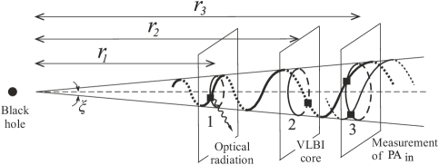
Figure 1: Schematic of the arrangement of regions in the jet in which the observed optical and radio emission arise and the region in which PA${}_{\text{in}}$ becomes measureable (the regions where a jet component crosses the circles 1, 2, and 3, respectively). The helical jet (without details of its components) is presented at a specified time by the thick bold curve. The thin curve shows the position of part of the jet in the vicinity of circle 3 at some subsequent time. We can see that the point where the jet crosses circle 3 shifts with time (similarly for circles 1 and 2). Over the variability periods for the optical emission, radio emission or PA${}_{\text{in}}$, these points undergo a full revolution about circles 1, 2, and 3, respectively.

2.1 Radial Motion of the Jet Components

We will first consider the case when the jet components move outward along the generating cone (so-called radial, or ballistic motion, see Fig. 2). Without loss of generality, we can assume that the difference in the azimuth angles of each of two successive components is some value $\varphi_{d}$ in radians. We denote $\Delta t^{\prime}_{1}$ to be the time interval in the comoving frame between the times when any two successive components cross circle 1. Over this time, a notional point moving along circle 1 describes an arc with length $\varphi_{d}$. For simplicity, we assumed that $2\pi$ is a multiple of $\varphi_{d}$. In this case, some number $n$ of components cross circle 1 over the rotation period of the notional point. Since the interval between two events in the observer’s frame is smaller than the interval in the source rest frame by a factor $\delta$,

$$\Delta t^{\prime}=\delta\Delta t,$$ (3)

the variability period for the optical emission in the observer’s frame will be

$$P_{1}=\sum_{j=1}^{n}\frac{\Delta t^{\prime}_{1}}{\delta\left(\theta\left(\varphi\right)\right)}\approx\frac{n\Delta t^{\prime}_{1}}{\delta\left(\theta_{0},\beta\right)}.$$ (4)

The right-hand side of (4) was obtained as follows. The angle $\theta$ of the components crossing circle 1 over the period varies from $\theta_{0}-\xi$ to $\theta_{0}+\xi$, where $\theta_{0}$ is the angle between the cone axis and the line of sight. According to formula (2), the Doppler factor varies cyclically in some interval. Deviations of the Doppler factor from its mean value can be neglected, since their magnitudes are not large, due to the smallness of the angle $\xi$, and their sum over the period is zero. For our further estimates, we took the mean Doppler factor to be $\delta\left(\theta_{0},\beta\right)$.

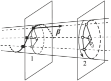
Figure 2: Schematic for interpreting the variability periods in the case of ballistic motion of the jet features. Part of the helical jet in the vicinity of the circle 1 is shown by the bold curve. The filled squares represent several jet components. The trajectories of each of the components lie along the generator of the cone (dashed curves). The hollow squares show the positions where these components will intersect the circles 1 and 2. The arrow indicates the direction of motion of a notional point along the circle 2 (similarly for the circle 1).

Moving farther, the component crosses circle 2. The variability period for the radio emission $P_{2}$ can be written similarly to (4), but with the subscript “1” replaced with “2”. Due to the character of the motion (Fig. 2), the azimuthal angle of each jet component does not vary with time. The number of components crossing circles 1 and 2 during the variation period $\varphi$ is also constant. The time intervals between the moments of intersection by two successive components of circles 1 and 2 are equal $\left(\Delta t^{\prime}_{1}=\Delta t^{\prime}_{2}\right)$. In the absence of deceleration of the components, we should have $P_{2}=P_{1}$. Since this is not observed, we supposed that the speed of the components crossing circle 2 was $\beta_{2}=a\beta_{1}$. Here, $0<a<1$ and $a>\beta_{2}$ (otherwise, $\beta_{1}>1$). It follows from (4) that the ratio of the variability periods in the optical and radio will be

$$\frac{P_{1}}{P_{2}}=\frac{\delta\left(\theta_{0},\beta_{2}\right)}{\delta\left(\theta_{0},\beta_{1}\right)}.$$ (5)

We used (2) and (5) to write the equation

$$\frac{1-\beta_{1}\cos\theta_{0}}{1-a\beta_{1}\cos\theta_{0}}\sqrt{\frac{1-a^{2}\beta_{1}^{2}}{1-\beta_{1}^{2}}}=\frac{P_{1}}{P_{2}},$$ (6)

which was solved numerically for $a$ for values $\beta_{1}=0.3-0.9999$ (corresponding to Lorentz factors $\Gamma=1-70$) with $P_{1}=3.3$ yrs and $P_{2}=5.8$ yrs.

We found that one root is always greater than one. The other root is negative when $\beta_{1}<0.52$ and satisfies our conditions when $\beta_{1}\geqslant 0.52$. When $a\approx 0.962$ and $\beta_{1}=0.9948$, the maximum value $\beta_{2}\approx 0.957$ is reached, corresponding to $\Gamma=3.5$. Solving (6) for $P_{2}$ and the variation period for the position angle of the inner jet for this interval of $\beta_{1}$ values yields the maximum value $\beta_{2}=0.949$ (for $a\approx 0.954$ and $\beta_{1}=0.995$), which corresponds to $\Gamma=3.1$. Thus, agreement of the variability periods observed at difference distances from the jet base can be achieved when $\Gamma\sim 3-4$. This does not agree with the values $\Gamma\sim 10-20$ inferred from observations of superluminal motions of jet components in 0716+714 (see, e.g., Bach et al., 2005; Nesci et al., 2005; Pushkarev et al., 2009).

2.2 Non-Radial Motion of the Jet Components

Let us now consider a helical jet whose components move non-ballistically, i.e., at some angle to a radial trajectory. We denote $p$ to be the pitch angle (angle between the generating cone and the velocity vector of a jet component), and $\psi$ to be the angle between the tangent to the helix of the jet and the generating cone at a given point (Fig. 3). If $p=\psi$, the jet will appear stationary in space, and will always cross circles 1, 2, and 3 at the same points. In this case, there should be no periodic variability, since the angle $\theta$, and consequently the Doppler factor, do not change in the regions responsible for the observed quantities. If $p\neq\psi$, we will observe the jet helix rotating about its axis. Due to the conical geometry of the jet, the variations of the azimuth angle $\varphi$ decrease with increasing $r$. However, we are interested in variations of $\varphi$ at the constant distances $r_{i}$ from the cone apex to the circles $i$ corresponding to the regions making the main contributions to the optical ($i=1$) and radio ($i=2$) emission, and to the region where PA${}_{\text{in}}$ can be measured ($i=3$) (Fig. 1).

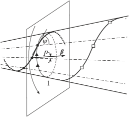
Figure 3: Schematic of a helical jet with non-ballistic motion of its components (shown by the filled squares). Part of the helical path of the jet located near circle 1 is shown (bold curve). The thin curves show the position of this part of the jet and the components at some later time, with $\psi\neq p$. The triangles on circle 1 show the places where the jet components cross circle 1. The arrows show the direction of motion of a notional point along circle 1.

Variations of the azimuthal angle of the part of the jet reaching a given distance $r_{i}$ from the cone apex can be found from the schematic presented in Fig. 4, under the condition that $\beta c\,dtr_{i}$:

$$d\varphi\approx\frac{\beta c\,dt\,\sin(\psi-p)}{r_{i}\sin\xi\cos\psi},$$ (7)

where $\xi$ is the opening angle of the cone ($\xi=1^{\circ}$, Butuzova, 2018). Since the angular frequency of a notional point moving along circle $i$ is $\omega_{i}=d\varphi/dt$, we find that the ratio of the periods of two observable quantities $i$ and $k$ is equal to the ratio of the distances from the cone apex to the region of the jet where these quantities are measured:

$$\frac{P_{i}}{P_{k}}=\frac{r_{i}}{r_{k}}.$$ (8)

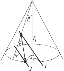
Figure 4: Schematic of part of the jet (bold curves) at a distance $r_{i}$ from the cone apex at the initial time (1) and after a time dt (2).

Substituting various pairs of the known variability periods for 0716+714 into (8) yields the three independent relations

$$\begin{split}r_{2}=&1.76\,r_{1},\\ r_{3}=&3.30\,r_{1},\\ r_{3}=&1.88\,r_{2}.\end{split}$$ (9)

It follows from the last two equations of (9) that $r_{2}/r_{1}\approx 1.76$, which is equal to the directly inferred ratio $r_{2}/r_{1}$ in the first equation of (9). Thus, the observed periods for the long-term variability in the ratio, optical and inner-jet position angle PA${}_{\text{in}}$ show good consistency. This supports a picture with non-radial motion of the jet features with $p\neq\psi$ and an absence of deceleration at the distances from the active nucleus considered here.

Let us suppose that PA${}_{\text{in}}$ is measured at a specified distance from the VLBI core at 15 GHz, equal to 0.15 mas. Then, $r_{3}-r_{2}=0.15$(mas)$/\sin\theta_{0}$. Using the third equation of (9) and $\theta_{0}=5.3^{\circ}$ (Butuzova, 2018), we obtain the distance $r_{2}=1.84$ mas. In a $\Lambda$CDM model with $H_{0}=71$ km s^-1Mpc^-1, $\Omega_{m}=0.27$, and $\Omega_{\Lambda}=0.73$ (Komatsu et al., 2009) and adopting a redshift of $z=0.3$ for 0716+714, the physical distance from the cone apex to the position of the VLBI core is 8.1 pc. This is consistent with the distance of the VLBI core from the black hole of 6.68 pc at 15.4 GHz determined by Pushkarev et al. (2012) using these same cosmological parameters. This provides additional support for our picture of the jet. Continuing our reasoning using (9), we find that the distance between the jet apex and the region where the optical emission becomes observable is 4.6 pc. Due to the small delay in the variability (at the limit of the time resolution of high frequency data of Rani et al., 2013; Larionov et al., 2013), we infer that the gamma-ray and optical emission is formed in the same region, or at least in closely spaced regions. Rani et al. (2014) estimated that the gamma-ray emission arises from a region located $3.8\pm 1.9$ pc closer to the black hole relative to the VLBI core (observed at 43 and 86 GHz), also consistent with our results.

3 Correlation between flux and inner-jet position angle

Assuming that the long-term variability of the blazar 0716+714 is due to periodic variations in the direction of motion of the jet components, we expect there should be a relationship between the measured spectral flux density $F_{\nu}$ and the inner-jet position angle. Such relationships between the gamma-ray flux $F_{\gamma}$ and both the flux from the VlBI core at 43 and 86 GHz and PA${}_{\text{in}}$ have been investigated for 0716+714 by Rani et al. (2014). They found that time intervals with a strong positive correlation between $F_{\gamma}$ and PA${}_{\text{in}}$ alternate with intervals in which there is a strong negative correlation between these two quantities.

This result was explained by Rani et al. (2014) by the fact that, in a curved (possibly helical) jet, the regions responsible for the observed quantities are located at different distances from the active nucleus, and therefore have different viewing angles $\theta$. If the $\theta$ values for two regions are roughly the same, there will be a strong positive correlation between the corresponding observed quantities. If the $\theta$ values are different, there may be a strong negative correlation. However, for the helical jet we are considering here, there is no direct relationship between $F_{\nu}$ and PA${}_{\text{in}}$, which can be explained as follows. According to Butuzova (2018) (Eq. (1)), the position angle is

$$\text{PA}_{\text{in}}=\text{PA}_{0}+\Delta\text{PA}=\text{PA}_{0}+\frac{\sin\xi\sin\varphi}{\cos\xi\sin\theta_{0}+\sin\xi\cos\theta_{0}\cos\varphi}$$ (10)

(PA₀ is the mean value of PA${}_{\text{in}}$) and the angle between the component velocity and the line of sight depend on the geometrical parameters of the cone and the position of the component relative to the cone axis and the line of sight (i.e., on the angle $\varphi$). We can use these equations, where the periodicity appears only due to variations in the azimuthal angle, to model the observed correlation between the flux and PA${}_{\text{in}}$.

Let us first consider the case of radialmotion of the components. We find from (1) with the substitution of (2), in which (see Butuzova, 2018, Eq. (5))

$$\theta=\theta_{b}=\arccos\left(\cos\xi\cos\theta_{0}-\sin\xi\sin\theta_{0}\cos\varphi\right),$$

that the extrema of the function $F_{\nu}$ occur at values $\varphi=n\pi$ (maxima for $n=1$, 3, 5, etc. and minima for $n=0$, 2, 4, etc.). That is, the qualitative variations of $F_{\nu}$ do not depend on the choice of $\nu$, $\alpha$, $s$, and $\beta$. The upper panel of Fig. 5 presents the variations of $F_{\nu}$ calculated using (1) and (10) (for $\alpha=0.5$, $s=2$, and $\beta=0.995$, which corresponds to $\Gamma=10$) and deviations of the inner-jet position angle from its mean value $\Delta$PA (for $\theta_{0}/\xi=5.3$) as functions of the azimuthal angle $\varphi$. The flux is normalized so as to enable a visual comparison of its variations with the variations of $\Delta$PA. The resulting curves were divided into several sections in $\varphi$, such that qualitative variations in the behavior of both quantities did not arise within each section.

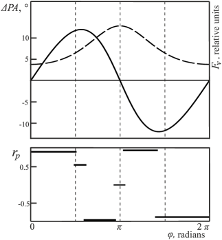
Figure 5: Deviations of the position angle of the inner jet from its mean value $\Delta$PA (solid curve) and the observed flux $F_{\nu}$ (dashed curve) over the variation period for $\varphi$ (upper), and the correlation coefficient $r_{p}$ between these quantities (lower) for ballistic motion of features of a helical jet.

The corresponding formulae were used to compose datasets of $\Delta$PA and $F_{\nu}$ values for each section, for variations of $\varphi$ in steps of $0.5^{\circ}$, and the Pearson correlation coefficient ($r_{p}$) between these datasets was calculated. The resulting $r_{p}$ value will have its maximum possible value, since, in contrast to the observational data, there is no measurement error. An alternation of intervals of strong positive and negative correlations can be seen (Fig. 5, lower panel). Intermediate values of the correlation coefficient are present only in short intervals. This theoretical result is in qualitative agreement with the observations of the behavior of the gamma-ray flux and the inner-jet position angle considered by Rani et al. (2014). Thus, we found that, for the same flux value (corresponding to the same viewing angle $\theta_{b}$), either a positive or negative correlation with PA${}_{\text{in}}$ could be present in the observations.

In the case of non-radial component motions, the variations of the viewing angle are given by Eqs. (11)-(13) from (Butuzova, 2018), which we do not present here due to their unwieldiness. The extrema of the function $F_{\nu}$ occur at the values

$$\varphi=-\arcsin\left(\frac{\sin p}{\sqrt{\cos^{2}p\sin^{2}\xi+\sin^{2}p}}\right)+\pi n,$$ (11)

where even $n$ correspond to maxima and odd $n$ to minima of the function $F_{\nu}$. According to (11), for the pitch angle found by Butuzova (2018) of $p=5.5^{\circ}$, the flux reaches a maximum when $\varphi\approx 100^{\circ}$. As $p$ is decreased, the peak $F_{\nu}$ shifts toward 180^∘, and the maximum $F_{\nu}$ occurs for $\varphi\approx 90^{\circ}$ when $p>20^{\circ}$. The upper panel of Fig. 6 plots the functions $F_{\nu}$ and $\Delta$PA for the same parameters as in the previous case. The correlation coefficient $r_{p}$ was constructed using an analogous procedure (Fig. 6, middle panel). This figure shows that a strong positive correlation between the inner jet position angle and the observed flux should always be present. However, since these quantities arise in regions located at different distances from the jet base in our model (see Section 2), we can conclude with confidence that the azimuthal angles of the components for which $F_{\nu}$ and $\Delta$PA are observed at a given time differ by some amount $\Delta\varphi$.

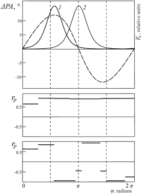
Figure 6: Upper: variations of the inner-jet position angle relative to the mean value $\Delta$PA (dashed curve) and of the flux $F_{\nu}$ for the case of zero difference in the azimuthal angles of the regions responsible for the observed quantities (curve 1) and for $\Delta\varphi\approx 79^{\circ}$ (curve 2). The central and lower panels show the correlation coefficients $r_{p}$ for the former and latter cases, respectively.

Agreement with the results of Rani et al. (2014) requires that this difference be $\Delta\varphi\approx 79^{\circ}$ (curve 2 for $F_{\nu}$ in the upper panel and curve for $r_{p}$ in the lower panel in Fig. 6). On the other hand, strong positive or negative correlations between $F_{\nu}$ and $\Delta$PA are also possible for radial component motions if the difference in the azimuthal angles is $\Delta\varphi\approx\pi/2$ or $\approx\pi$ (see Fig. 5). Consequently, the correlation between the observed quantities may be insignificant when analyzing data over long time intervals, as was found by Raiteri et al. (2003), for example, in their analysis of the radio and optical fluxes during 1994$-$2001. In contrast, the data for the shorter interval 2007$-$2010 analyzed by Rani et al. (2013) revealed a correlation between the indicated quantities at a significance level of more than 99$\%$. Further, the difference in the azimuthal angles of the regions responsible for the observed quantities can appreciably affect both the correlation coefficient between PA${}_{\text{in}}$in and $F_{\nu}$ and the duration of the time interval when a given correlation coefficient is observed. Finally, the character of the motions of individual components of helical jet cannot be determined by analyzing the correlation between PA${}_{\text{in}}$ and $F_{\nu}$. It is important to note that, when investigating correlations between fluxes observed in different spectral ranges, distinct correlation coefficients in the different time intervals will also be present.

4 Discussion and conclusion

The hypothesis that AGN jets may be helical has been widely applied for several decades to interpret various observed properties such as their microvariability (Camenzind & Krockenberger, 1992), the shape and variations of the spectral energy distributions for the blazars Mrk 501 (Villata & Raiteri, 1999) and 0716+714 Ostorero et al. (2001), the long-term brightness variability of OJ 287 (Sillanpaa et al., 1988) and 0716+714 (Nesci et al., 2005), variations in the speeds and non-radial component motions (Rastorgueva et al., 2009), and quasi-periodicity of variations of the inner-jet position angle for 0716+714 (Bach et al., 2005; Lister et al., 2013). A helical jet shape could form due to precession of the jet nozzle or the development of (magneto)hydrodynamical instabilities. Kelvin–Helmholtz instability (Hardee, 1982) has been widely studied as a means of estimating the physical parameters of jets and the ambient medium (e.g., for 3C 120 (Hardee, 2003) and 0836+710 (Perucho et al., 2012)). Alternatively, wavelike perturbations at the boundaries of the observed isophotes of jets could be related to the development of a magnetohydrodynamical analog of wind instability (Gestrin & Kontorovich, 1986).

In this study, we have supposed that the radiating jet components form a helical curve, without considering their physical nature. For example, the jet components could be individual radiating parts of the jet (plasmoids or regions of shocks) or volume elements (in the case of a spatially continuous radiating jet). A helical shape suggests the presence of periodic variations of the angle between the jet velocity and the line of sight at some constant distance from the core, which should be manifest as long-term quasi-periodic variability of the radiation flux over the entire observed range of the electromagnetic spectrum of the blazar 0716+714. The differences in the quasi-periods for the variations of PA${}_{\text{in}}$ (Bach et al., 2005; Lister et al., 2013) and of the radio- (Raiteri et al., 2003; Bychkova et al., 2015; Bach et al., 2005; Liu et al., 2012) and optical (Raiteri et al., 2003) fluxes can most simply be explained in the jet geometry considered if the radiation in different spectral ranges is emitted at different distances from the jet apex. This spatial separation of regions radiating at different frequencies can arise due to synchrotron self-absorption in the jet or the energy losses of the radiating electrons. In both cases, the higher the frequency of the observed emission, the closer to the jet base the region in which it is generated. The delays in the flux variability observed at different frequencies also testify to the action of this effect (see, e.g., Raiteri et al., 2003; Larionov et al., 2013; Rani et al., 2014).

In this study, we have brought the variability periods in different spectral ranges into agreement in the case of radial and non-radial motions of the radiating components. The former case requires a low Lorentz factor for the components (no more than 4) with overall deceleration, at least from the region where the optical emission is formed to 0.15-0.5 mas from the core, where the position angle of the inner jet is measured. This does not agree with observations of features in the parsec-scale jet of 0716+714 (Bach et al., 2005; Nesci et al., 2005; Pushkarev et al., 2009). Moreover, it was shown by Butuzova (2018) that differences between the relative speeds of components in the inner and outer jet observed in different years can be explained in the framework of a helical-jet model with non-ballistic component motions, such as are observed in the jet (Bach et al., 2005; Rastorgueva et al., 2009). It was shown that period ratio is equal to ratio of the physical distances from the jet apex of the regions responsible for the measured quantities. This enables us to introduce another absolute distance scale, which will subsequently facilitate deeper studies of the jet properties. In our picture of the jet and the appearance of long-term variability due to geometric effects, the radio periods found by Bychkova et al. (2015) cannot carry information about the properties of the central engine without taking into account the non-radial motions of the jet components.

The helical shape of a jet with spatially separated regions responsible for the observed emission at different frequencies and region where the inner jet position angle is measured complicates studies of correlations between the observed quantities. It has been shown that there cannot be a constant correlation coefficient between quantities formed in regions at different fixed distances from the jet apex. A strong positive correlation observed in one time interval will be replaced with a negative correlation in another. This is due to both the different azimuthal angles of these regions and the fact that $\varphi$ varies irregularly in the observer’s rest frame, due to variations of $\delta$, especially for non-radial component motions (Butuzova, 2018). This agrees with certain observational facts.

For example, Rani et al. (2013) noted an alternation of intervals when positive and negative correlations between PA${}_{\text{in}}$ and the gamma-ray flux of the blazar 0716+714 were observed. Rani et al. (2013) also indicate that a strong correlation between the gamma-ray and optical fluxes was observed over roughly 500 days (Pearson correlation coefficient $r_{p}=0.66$), while $r_{p}=0.36$ over the following $\approx$400 days. A correlation was also found between the radio flux and PA${}_{\text{in}}$ during 1994$-$2014 ($r_{p}=0.44$) (Liu et al., 2012), while no correlation between these quantities was found for data obtained from August 2008 through September 2013 (Rani et al., 2014).

We can introduce some clarity into this picture only if we know the geometrical parameters of the helical jet, the character of the motion of the jet components,and the arrangement of the studied regions responsible for various observed quantities relative to the plane containing the axis of the helical jet and the line of sight, and not only relative to the line of sight, as was supposed in the simplest case (Rani et al., 2014). We also showed in Section 3 that it is not possible to determine the character of the component motions in a helical jet based on the correlation between the radio flux and the inner-jet position angle, as was done by Liu et al. (2012).

Our hypothesis that the jet of the blazar 0716+714 has the form of a helical curve located on the surface of a cone may seem somewhat idealized. However, this is consistent with the results of many years of VLBI observations (Lister et al., 2013; Pushkarev et al., 2017). In addition, a helical jet with non-radial component motions makes it possible to find agreement between estimates of the component velocities in the VLBI jet and the viewing angle obtained in different studies, which often differ appreciably (Butuzova, 2018). As we have shown, such a jet can provide a simple explanation for the differences in the observed long-term quasi-periods for different quantities, as well as the differences in the correlations between the observed quantities in different time intervals.

References

- Agarwal et al. (2017) Agarwal, A., Mohan, P., Gupta, A. C., et al. 2017, MNRAS, 469, 813, doi: 10.1093/mnras/stx847
- Bach et al. (2005) Bach, U., Krichbaum, T. P., Ros, E., et al. 2005, A&A, 433, 815, doi: 10.1051/0004-6361:20040388
- Butuzova (2018) Butuzova, M. S. 2018, Astronomy Reports, 62, 116, doi: 10.1134/S1063772918020038
- Bychkova et al. (2006) Bychkova, V. S., Kardashev, N. S., Boldycheva, A. V., Gnedin, Y. N., & Maslennikov, K. L. 2006, Astronomy Reports, 50, 802, doi: 10.1134/S1063772906100040
- Bychkova et al. (2015) Bychkova, V. S., Vol’vach, A. E., Kardashev, N. S., et al. 2015, Astronomy Reports, 59, 851, doi: 10.1134/S1063772915080016
- Camenzind & Krockenberger (1992) Camenzind, M., & Krockenberger, M. 1992, A&A, 255, 59
- Danforth et al. (2013) Danforth, C. W., Nalewajko, K., France, K., & Keeney, B. A. 2013, ApJ, 764, 57, doi: 10.1088/0004-637X/764/1/57
- Edelson & Krolik (1988) Edelson, R. A., & Krolik, J. H. 1988, ApJ, 333, 646, doi: 10.1086/166773
- Gestrin & Kontorovich (1986) Gestrin, S. G., & Kontorovich, V. M. 1986, Soviet Astronomy Letters, 12, 220
- Gorshkov et al. (2011) Gorshkov, A. G., Ipatov, A. V., Konnikova, V. K., et al. 2011, Astronomy Reports, 55, 97, doi: 10.1134/S106377291102003X
- Hardee (1982) Hardee, P. E. 1982, ApJ, 257, 509, doi: 10.1086/160008
- Hardee (2003) —. 2003, ApJ, 597, 798, doi: 10.1086/381223
- Komatsu et al. (2009) Komatsu, E., Dunkley, J., Nolta, M. R., et al. 2009, ApJS, 180, 330, doi: 10.1088/0067-0049/180/2/330
- Kovalev et al. (2008) Kovalev, Y. Y., Lobanov, A. P., Pushkarev, A. B., & Zensus, J. A. 2008, A&A, 483, 759, doi: 10.1051/0004-6361:20078679
- Kudryavtseva et al. (2011) Kudryavtseva, N. A., Gabuzda, D. C., Aller, M. F., & Aller, H. D. 2011, MNRAS, 415, 1631, doi: 10.1111/j.1365-2966.2011.18808.x
- Larionov et al. (2013) Larionov, V. M., Jorstad, S. G., Marscher, A. P., et al. 2013, ApJ, 768, 40, doi: 10.1088/0004-637X/768/1/40
- Liao et al. (2014) Liao, N. H., Bai, J. M., Liu, H. T., et al. 2014, ApJ, 783, 83, doi: 10.1088/0004-637X/783/2/83
- Lister et al. (2013) Lister, M. L., Aller, M. F., Aller, H. D., et al. 2013, AJ, 146, 120, doi: 10.1088/0004-6256/146/5/120
- Liu et al. (2012) Liu, X., Mi, L., Liu, B., & Li, Q. 2012, Ap&SS, 342, 465, doi: 10.1007/s10509-012-1191-6
- Lobanov (1998) Lobanov, A. P. 1998, A&A, 330, 79. https://arxiv.org/abs/astro-ph/9712132
- Marcaide & Shapiro (1984) Marcaide, J. M., & Shapiro, I. I. 1984, ApJ, 276, 56, doi: 10.1086/161592
- Nesci et al. (2005) Nesci, R., Massaro, E., Rossi, C., et al. 2005, AJ, 130, 1466, doi: 10.1086/444538
- Nilsson et al. (2008) Nilsson, K., Pursimo, T., Sillanpää, A., Takalo, L. O., & Lindfors, E. 2008, A&A, 487, L29, doi: 10.1051/0004-6361:200810310
- Ostorero et al. (2001) Ostorero, L., Raiteri, C. M., Villata, M., et al. 2001, Mem. Soc. Astron. Italiana, 72, 147
- Perucho et al. (2012) Perucho, M., Kovalev, Y. Y., Lobanov, A. P., Hardee, P. E., & Agudo, I. 2012, ApJ, 749, 55, doi: 10.1088/0004-637X/749/1/55
- Poon et al. (2009) Poon, H., Fan, J. H., & Fu, J. N. 2009, ApJS, 185, 511, doi: 10.1088/0067-0049/185/2/511
- Pushkarev et al. (2012) Pushkarev, A. B., Hovatta, T., Kovalev, Y. Y., et al. 2012, A&A, 545, A113, doi: 10.1051/0004-6361/201219173
- Pushkarev et al. (2009) Pushkarev, A. B., Kovalev, Y. Y., Lister, M. L., & Savolainen, T. 2009, A&A, 507, L33, doi: 10.1051/0004-6361/200913422
- Pushkarev et al. (2017) —. 2017, MNRAS, 468, 4992, doi: 10.1093/mnras/stx854
- Raiteri et al. (2003) Raiteri, C. M., Villata, M., Tosti, G., et al. 2003, A&A, 402, 151, doi: 10.1051/0004-6361:20030256
- Rani et al. (2014) Rani, B., Krichbaum, T. P., Marscher, A. P., et al. 2014, A&A, 571, L2, doi: 10.1051/0004-6361/201424796
- Rani et al. (2013) Rani, B., Krichbaum, T. P., Fuhrmann, L., et al. 2013, A&A, 552, A11, doi: 10.1051/0004-6361/201321058
- Rastorgueva et al. (2009) Rastorgueva, E. A., Wiik, K., Savolainen, T., et al. 2009, A&A, 494, L5, doi: 10.1051/0004-6361:200811425
- Sbarufatti et al. (2005) Sbarufatti, B., Treves, A., & Falomo, R. 2005, ApJ, 635, 173, doi: 10.1086/497022
- Sillanpaa et al. (1988) Sillanpaa, A., Haarala, S., Valtonen, M. J., Sundelius, B., & Byrd, G. G. 1988, ApJ, 325, 628, doi: 10.1086/166033
- Simonetti et al. (1985) Simonetti, J. H., Cordes, J. M., & Heeschen, D. S. 1985, ApJ, 296, 46, doi: 10.1086/163418
- Villata & Raiteri (1999) Villata, M., & Raiteri, C. M. 1999, A&A, 347, 30
- Volvach et al. (2012) Volvach, A. E., Volvach, L. N., Bychkova, V. S., et al. 2012, Astronomy Reports, 56, 275, doi: 10.1134/S1063772912030079
- Wagner et al. (1996) Wagner, S. J., Witzel, A., Heidt, J., et al. 1996, AJ, 111, 2187, doi: 10.1086/117954
- Wu et al. (2007) Wu, J., Zhou, X., Ma, J., et al. 2007, AJ, 133, 1599, doi: 10.1086/511773