Abstract

There is often variation in the shape and size of input data used for deep learning. In many cases, such data can be represented using tensors with non-uniform shapes, or ragged tensors. Due to limited and non-portable support for efficient execution on ragged tensors, current deep learning frameworks generally use techniques such as padding and masking to make the data shapes uniform and then offload the computations to optimized kernels for dense tensor algebra. Such techniques can, however, lead to a lot of wasted computation and therefore, a loss in performance. This paper presents CoRa, a tensor compiler that allows users to easily generate efficient code for ragged tensor operators targeting a wide range of CPUs and GPUs. Evaluating CoRa on a variety of operators on ragged tensors as well as on an encoder layer of the transformer model, we find that CoRa (i) performs competitively with hand-optimized implementations of the operators and the transformer encoder and (ii) achieves a $1.6\times$ geomean speedup for the encoder on an Nvidia GPU over PyTorch and a $1.37\times$ geomean speedup for the multi-head attention module used in transformers on a 64-core ARM CPU over TensorFlow.

1 Introduction

Deep learning (DL) is used for a variety of computational tasks on different kinds of data including sequential data like text treelstm; transformer, audio wavenet and music music_dl; music_trans and spatial data like images resnet. Simultaneously, DL models have become more and more computationally expensive. More efficient execution of these models is, therefore, a priority.

Figure 1: An example operation on ragged tensors.

There is often variation in the sizes of the data that we process using DL. Images can be of different resolutions, textual sentences and documents can be of different lengths, and audio can be of different durations. Processing such data exhibiting variation in shape, or shape dynamism nimble, using the same model and further, as part of the same mini-batch is therefore important. An example elementwise operation on such data is shown in Fig. 1, where the slices of the inner dimension of tensor A have variable sizes. Such tensors and operators are referred to as ragged tensors and ragged operators respectively. Note how the shape dynamism translates to a variable bound for loop L2 which iterates over the variable-sized tensor slices.

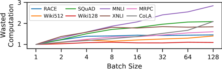
Figure 2: Wasted computation due to padding in a transformer encoder layer.

Past work has developed hand-optimized kernels to accelerate some important ragged applications such as batched matrix multiplication with variable dimensions cbt; magma, triangular matrix multiplication trmm and the widely-used transformer transformer models EffectiveTrans; FT. Such hand-optimized kernels, however, require substantial development effort and, hence, are available only for a few operators. Further, they are not portable across different hardware substrates, which is problematic due to the rapid innovation in DL hardware.

While some DL frameworks have started providing support for ragged operators recently TFRagged; PTNested, it is quite limited TFIssue; PTIssue; NTL as discussed in §LABEL:sec:related. Therefore, frameworks usually rely on efficient dense tensor algebra kernels implemented in vendor libraries such as cuDNN cudnn and oneDNN onednn or generated by tensor compilers such as TVM tvm to target parallel hardware. Padding (illustrated in the top right of Fig. 1) and masking are therefore commonly used to eliminate shape dynamism in ragged tensors and enable the use of vendor libraries or dense tensor compilers HuggingFacePadding.

Padding and masking, however, lead to wasted computation as the padding or the masked data points are discarded after execution. Fig. 2 plots the relative amount of computation (computed analytically in FLOPs) involved in the forward pass of an encoder layer of the transformer model with and without padding. We see that padding leads to a significant increase in the computational requirements of the layer, especially at larger batch sizes, increasing computation in an already computationally expensive model.

Thus, current solutions for efficient ragged operator execution are unsatisfactory. Hence, we propose a compiler-based solution enabling easy and more portable generation of performant code for ragged operators. While sparse comet; taco and dense tvm; tc; halide; tiramisu tensor compilers have been well-studied, it is not straightforward to apply these techniques to ragged tensors, due to the following challenges:

1. Irregularity in generated code: While the data in ragged tensors are densely packed, the variable loop bounds can lead to irregular code, often causing a loss of performance on hardware substrates such as GPUs.

2. Insufficient compiler mechanisms: Representing transformations on loops with variable bounds and on tensor dimensions with variable-sized slices is not straightforward due to the dependencies that exist among loops and tensor dimensions respectively in ragged operators. Further, optimization decisions made by sparse tensor compilers may not always work for ragged tensors as sparse tensors are much sparser than ragged tensors.

3. Ill-fitting computation abstractions: There is a mismatch between the interfaces and abstractions provided by current compilers and ragged operators. Such operators cannot be expressed in dense compilers, while sparse compilers do not adequately provide ways to express information relevant to efficient code generation.

Table 1: Comparison between CoRa and current solutions for ragged operations. TC stands for tensor compilers.

Framework	Portability	Operator impl. effort	Padding	Performance
Dense TC	High	Low	Full	Low
Sparse TC	High	Low	Minimal	Low
Dense vendor libs.	Low	High	Full	Low
Hand-optimized impl.	Low	High	Minimal	High
CoRa	High	Low	Minimal	High

With these challenges in mind, we present CoRa (Compiler for Ragged Tensors), a tensor compiler which allows one to express and optimize ragged operations to easily target a variety of substrates such as CPUs and GPUs. To overcome challenge C1, CoRa enables minimal padding of ragged tensor dimensions (§4.1) in order to generate efficient code for targets such as GPUs as well as to specify thread remapping strategies to lower load imbalance (§4.1). CoRa uses uninterpreted functions spf1 to symbolically represent variable loop bounds and scheduling operations on the same (§5.1). CoRa’s mechanisms (such as its storage lowering scheme discussed in §5.3) and optimizations are specialized for ragged tensors thereby tackling C2. Further, CoRa provides simple abstractions to convey information essential to efficient code generation such as padding or thread remapping specifications and raggedness patterns of tensors to the compiler (§4). This overcomes challenge C3.

CoRa enables efficient code generation for ragged operators by significantly reducing padding (§7). As part of CoRa’s implementation, we reuse past work by extending a tensor compiler halide; tvm; tiramisu; taco and thus, provide familiar interfaces to CoRa’s users. This also makes it easy in the future to use auto-scheduling halide_auto1; halide_auto2; tvm_autotune; ansor; auto_sched10 for optimizing ragged tensor operations. Table 1 compares CoRa with alternatives that are or could be used for ragged operators. Only CoRa achieves high performance and portability, with low operator implementation effort (and minimal padding).

In summary, this paper makes the following contributions:

1. We present CoRa, a tensor compiler for ragged tensors. To our knowledge, CoRa is the first tensor compiler that allows efficient computation on ragged tensors.

2. As part of the design, we generalize the API, abstractions and the mechanisms of tensor compilers and propose new scheduling primitives for ragged tensors.

3. We evaluate CoRa on a variety of ragged operators. For a transformer encoder layer, we perform $1.6\times$ better than PyTorch PyTorch and as well as FasterTransformer FT, a highly optimized transformer implementation, on an Nvidia V100 GPU. On a 64-core ARM CPU, we are $1.37\times$ faster than TensorFlow TensorFlow, for the multi-head attention (MHA) module transformer used in transformers.

2 CoRa Overview

CoRa’s compiler-based approach enables the generation of performant code in a portable manner. This is reflected in Fig. 3, which compares CoRa’s implementation of a transformer encoder layer with FasterTransformer. The highly-optimized FasterTransformer relies heavily on kernels implemented in cuBLAS (Nvidia’s BLAS library), which are shown as blue outlines in the figure, and on manually implemented kernels, shown as red outlines. On the other hand, CoRa’s implementation exclusively employs compiler generated kernels (shown as green outlines), making it more portable. Further, CoRa’s compiler approach allows it to exploit more kernel fusion opportunities, evident from the fact that CoRa’s implementation launches nine kernels as opposed to FasterTransformer’s twelve. Both the implementations in the figure use minimal padding for all operators except for those in the scaled dot-product attention (SDPA) sub-module, where CoRa’s specialized approach enables it to get away with lower padding as compared to FasterTransformer. We further discuss these implementations in §7.

Figure 3: FasterTransformer (FT-Eff) and CoRa implementations of a transformer’s encoder layer. Note how CoRa’s fully compiler-based implementation uses only partial padding for SDPA as opposed to FasterTransformer’s fully padded implementation. CoRa also enables more operator fusion (including fusing all the padding change operations) as opposed to FasterTransformer, which cannot do so in all cases as it relies on vendor libraries.

CoRa’s ability to generate performant code that employs minimal padding in a portable manner as we saw above relies on the following two insights:

1. In ragged operations, the pattern of raggedness is usually known before the tensor is actually computed, and is the same across multiple tensors involved in the operation.

2. Ragged tensors, like dense tensors, allow $O(1)$ accesses (§5.3). This is unlike sparse formats such as compressed sparse row (CSR), where accesses require a search over an array. The HASH taco_format sparse format, while allowing $O(1)$ accesses, is unsuitable for accelerators such as GPUs due to its highly irregular storage.

Insight I1 allows CoRa to precompute the auxiliary data structures needed to access ragged tensors without knowledge of the computation (or values of its input tensors) that produces the ragged tensor. This and insight I2 enable CoRa to generate efficient code for ragged operations.

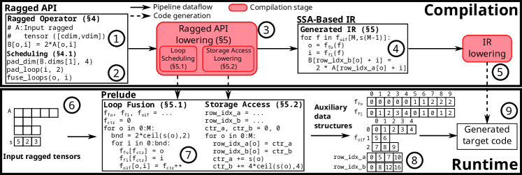
Figure 4: Overview of CoRa’s compilation and runtime pipeline.

Let us now look at CoRa’s overall compilation and execution pipeline, as illustrated in Fig. 4. The user first expresses and schedules their computation using an API similar to that of past tensor compilers (§4). This specification of the computation and the scheduling primitives are then lowered to an SSA-based IR . As part of this lowering step, CoRa generates code to initialize some auxiliary data structures it needs to be able to lower accesses to ragged tensors (§5.3) and to enable loop fusion in ragged loop nests (§5.1). We refer to this code as the prelude code. Compilation then continues with CoRa lowering tensor accesses to raw memory offsets by making use of the data structures generated by the prelude. Finally, CoRa generates target-dependent code such as C or CUDA C++. During execution, the formats of the input ragged tensors are first processed by the generated prelude code which creates the auxiliary data structures . This prelude code is not computationally expensive (§7.4) and hence is executed on the host CPU. These data structures and the ragged tensors are then passed to the generated target dependent code which executes on devices such as CPUs or GPUs.

We will now look these stages in more detail below.

3 Terminology

Ragged operators have one or more loops with bounds that are functions of iteration variables of outer loops. We refer to such loops as variable loops or vloops while loops with constant bounds are referred to as constant loops, or cloops. A loop nest with at least one vloop is referred to as a vloop nest. Further, tensors can be stored in memory with or without padding. When stored without full padding, the size of some tensor dimensions depends on outer tensor dimensions. Such dimensions are referred to as variable dimensions, or vdims and those with constant sizes are constant dimensions or cdims. A tensor stored such that it has no vdim (i.e. a fully padded tensor) is referred to as a dense tensor, while a tensor with at least one vdim is a ragged tensor. Note that ragged tensors may be padded to some extent.

4 CoRa’s Ragged API

CoRa provides a simple API similar to that of past tensor compilers, as seen in Listing 1, which expresses the example computation from Fig. 1 in CoRa. Apart from describing the computation as in a dense tensor compiler, CoRa also requires the user to specify the raggedness dependences of the computation (highlighted in Listing 1). This involves specifying vloop bounds as functions of outer loop variables and vdim extents as functions of indices of outer tensor dimensions. Given this information, CoRa automatically computes any derived data structures required (§5), making it easy for users to express their computations. CoRa uses identifiers called named dimensions (discussed further in §5.2) to name loops and corresponding tensor dimensions and to specify relationships between them. For example, the loop extent defined on line LABEL:line:lext in the listing states the dependence on the outer loop, referred to by the named dimension batch_dim.

⬇

1################ Operator Description ################

2batch_size = var(’M’)

3# Declare named dimensions

4batch_dim, len_dim = Dim(), Dim()

5# Loop: Specify vloop extents

6lens = input_tensor((batch_size,))

7l_ext = Extent([batch_dim], lambda b: lens[b])

8loop_exts = [batch_size, l_ext]

9# Storage: Specify vdim extents

10s_ext = Extent([batch_dim], lambda b: lens[b])

11storage_format = [batch_size, s_ext]

12# Define input ragged tensor

13dims = [batch_dim, len_dim]

14A = input_tensor(dims, storage_format)

15# Express computation

16B = compute(dims, loop_exts, lambda i,j: 2*A[i,j])

17############### Scheduling primitives ###############

18pad_loop(B.loops[1], 2)

19pad_dimension(B.dimensions[1], 4)

20fuse_loops(B.loops[0], B.loops[1])

Listing 1: Operator in Fig. 1 expressed in a simplified version of CoRa’s API.

4.1 Scheduling Primitives

In order to optimize the expressed computation, CoRa provides all the scheduling primitives commonly found in tensor compilers. Below, we describe some salient features and points of departure from past tensor compilers.

Loop Scheduling: Both cloops and vloops can be scheduled in CoRa. We saw how a vloop, say $L_{v}$, has a loop bound that is a function of the iteration variables of one or more outer loops, say $L_{1}$ to $L_{k}$. CoRa currently does not allow reordering such a loop $L_{v}$ beyond any of the loops $L_{1}$ to $L_{k}$. While possible with the introduction of conditional statements, we have not found a use case for such reordering.

Operation Splitting: It can sometimes be beneficial to differently schedule different iterations of a loop in a vloop nest in order to more optimally handle the variation in loop bounds. CoRa allows one to split an operation into two or more operations by specifying split points for one or more of its loops, as Fig. 5 shows. In our evaluation (§7.3), we use this transformation in conjunction with horizontal fusion (described below) to better handle the last few iterations of a tiled loop without the need for additional padding in the QK^T and AttnV operators in the transformer layer (Fig. 3).

Figure 5: Operation splitting and horizontal fusion. Loop L₂ is first split in step 1 using operation splitting thus creating two loop nests, which are then horizontally fused together (step 3) so they execute concurrently as part of single kernel.

Horizontal Fusion: Past work hfusion has proposed horizontal fusion, or hfusion for short, as an optimization to better utilize massively parallel hardware devices such as GPUs by executing multiple operators concurrently as part of a single kernel. With CoRa, we implement this optimization in a tensor compiler for the outermost loop of two or more operators. HFusion enables the concurrent execution of the multiple operators that result from using the operation splitting transform described above.

Loop and Storage Padding: Despite the overheads of padding, a small amount of it is often useful in order to generate efficient vectorized and tiled code by eliding conditional checks. Accordingly, CoRa allows the user to specify padding for vloops and vdims as multiples of a constant. For example, on line LABEL:line:lpad of Listing 1, the vloop associated with the dimension len_dim is asked to be padded to a multiple of 2 while the corresponding dimension of the output tensor is specified to be padded to a multiple of 4 on line LABEL:line:spad. Such independent padding specification for loops and the underlying storage is allowed as long as the storage padding is at least as much as the loop padding (this ensures that the padded loop nest never accesses non-existent storage). This ability allows CoRa to fuse padding change operators as is illustrated in Fig. 3. We show in §7.4 that this partial padding does not lead to much wasted computation.

Tensor Dimension Scheduling: CoRa allows users to split, fuse and reorder dimensions of dense and ragged tensors. This can enable more optimal memory accesses. Fusing tensor dimensions in a way that mirrors the surrounding loop nest can allow for simpler memory accesses (§5.1).

Load Balancing: The variable loop bounds in a vloop nest can lead to unbalanced load across execution units. As proposed by past work dl_sparse on sparse tensor algebra, CoRa allows the user to redistribute work across different parallel processing elements by specifying a thread remapping policy. Given a parallel loop, this allows the user to specify a mapping between the loop iterations and the thread id (illustrated in Fig. LABEL:fig:ap_thread_remap in the appendix). Depending on the hardware thread scheduling policy, this can influence the order in which iterations of the loop are scheduled and lead to non-trivial performance gains as shown in §7.1.

In conclusion, CoRa provides familiar and simple interfaces to users, extended with a few abstractions and scheduling primitives specific to ragged tensors, enabling their application to support (efficient) ragged operations.

5 CoRa’s Ragged API Lowering

We now discuss some aspects of CoRa’s Ragged API lowering that generates the SSA-based IR as shown in Fig 4.

5.1 Loop and Tensor Dimension Fusion

Consider the ragged loop nest shown on the top left corner of Fig 6. The loop bound of the inner loop L_i is a function $s()$ of o, the iteration variable of the outer loop L_o. The loop L_f obtained by fusing L_o and L_i is shown on the right of the figure. The loop bound F of the fused loop would be equal to $\sum_{o=0}^{M-1}s(o)$. Further note that while we have fused the loops L_o and L_i, the tensor access T[o,i] in the body of the loop nest still uses variables o and i. Therefore, we need to compute the values of these two variables corresponding to the current value of f, the iteration variable of L_f. Because of the ragged nature of the loop nest, computing the loop bound F as well as the mapping between the iteration variables of the original and the fused loop nests is not straightforward. In CoRa, we generate code to compute these quantities and variable relationships (shown in the right pane of Fig. 6) as part of the prelude which executes before the main kernel computation. We use vloop fusion as described above to implement the linear transformation operators (Proj1, Proj, FF1 and FF2) in the transformer encoder (Fig. 3) with minimal padding.

Suppose now that the tensor T in Fig. 6 has a storage format that mirrors the loop nest consisting of L_o and L_i. This means that the 2-dimensional tensor has an outer cdim and an inner vdim the size of the $i^{th}$ slice of which is $s(i)$. Fusing these dimensions then enables CoRa to simplify the tensor access as shown in the bottom left pane of the figure.

Figure 6: Fusing vloops and tensor dimensions

5.2 Bounds Inference

Figure 7: Iteration variable ranges during vloop fusion.

Variable Loop Fusion: During compilation, a tensor compiler infers loop bounds for all operators. In order to do so, the compiler usually proceeds from the outputs of the operator graph towards the inputs, inferring the region of a tensor $t$ that needs to be computed and then using this information to infer the loop bounds for the operator that computes $t$. As we saw in §5.1, the application of scheduling transformations such as fusion can lead to a situation where the variables used in the tensor accesses in an operator’s body are not the same as the loop iteration variables present after the transformations have been applied. This means that during bounds inference, one has to repeatedly translate iteration variable ranges between the transformed and the original variables. This is straightforward in the case of cloops, but gets slightly harder in the case of vloop fusion. For the loop nest in Fig. 6, Fig 7 provides the rules to translate between the ranges of iteration variables o, i and f as well as a visualization of the ranges. Here, $s()$ represents the variable loop bound of the inner loop, while $f_{oif}$, $f_{fo}$ and $f_{fi}$ represent the relationships between the variables o, i and f such that $f_{fo}(f_{0})$ and $f_{fi}(f_{0})$ evaluate to values of o and i, respectively, corresponding to f$=f_{0}$. Similarly, $f_{oif}(o_{0},i_{0})$ evaluates to $f_{0}$.

Named Dimensions: In §4, we described how the user uses named dimensions to specify relationships between loops as well as tensor dimensions. These dimensions play an important part in bounds inference as well. Along with the translation between fused and unfused loop iteration variables described above, one also needs to translate ranges of variables across producers and consumers during bounds inference. In CoRa, we use named dimensions to easily identify corresponding iteration variables across such producers and consumers to allow this translation.

5.3 Storage Access Lowering

In this section, we briefly describe how CoRa lowers accesses to ragged tensors. Consider the 4-dimensional attention matrix $X$ involved in a batched implementation of MHA shown in the left pane of Fig. 8. Here, the first and the third dimensions are cdims and correspond to the batch size and the number of attention heads, respectively. The other two dimensions, corresponding to sequence lengths, are vdims. For $X$, the size of a slice for both these vdims is the same function ($s_{24}())$) of the outermost batch dimension.

Due to the irregular nature of ragged tensor storage, we need some auxiliary data structures to be able to lower memory accesses to $X$. The lowering scheme used by past work on sparse tensors csf; taco_format assumes that the number of non-zeros in a slice of a sparse dimension is, in general, a function of all outer dimensions. However, recall that for our example tensor $X$, the size of a slice of either vdim depends only on the outermost batch dimension. Being agnostic to such precise dependencies between tensor dimensions (as illustrated via the dimension graphs, or dgraphs in Fig. 8), past work would compute and store more auxiliary data as compared to CoRa.

CoRa’s lowering scheme allows for cheap $O(1)$ accesses to ragged tensors. To enable this, we need to compute a memory offset within a constant number of operations. The reason sparse tensor formats such as the CSR format do not allow constant time tensor accesses is because they explicitly store indices of one or more dimensions along with every non-zero value. Thus, given a tensor index, one needs to perform a search over these stored indices to obtain the correct non-zero element. In the case of ragged tensors, however, we note that within a vdim slice, the data in densely packed with no intervening zero elements. Therefore, we can get away without storing explicit indices for any dimension. Accessing the precomputed memory offsets is also a constant time operation as CoRa’s auxiliary data structures store these offsets using simple arrays.

Figure 8: CoRa precisely models dimension dependences as compared to past schemes for sparse tensors.

We describe these lowering schemes further in the appendix in §LABEL:sec:ap_access_lowering. In short, however, our storage access lowering scheme reduces the amount of auxiliary data that needs to be computed thus reducing overheads of the prelude code (§7.4), while allowing cheap tensor accesses.

6 Implementation

We prototype CoRa by extending TVM tvm v0.6, a DL framework and a tensor compiler. Some details regarding this implementation are discussed below.

Ragged API: Our prototype allows vdims to depend on at most one outer tensor dimension. This is not a fundamental limitation and can easily be overcome, though we have not needed to for our evaluation. We implement the operator splitting and hfusion transforms for non-reduction loops.

Lowering: Our current prototype does not auto-schedule the expressed computation. The evaluation therefore uses implementations optimized using a combination of manual scheduling and grid search. For some operators, we auto-scheduled the corresponding dense tensor operator using past work ansor and manually applied the schedule to the ragged case. We find that this works well in most cases and therefore believe that the prototype could readily be extended with prior work on auto-scheduling. Our implementation currently expects users to correctly allocate memory (taking into account padding requirements as specified in the schedule) for tensors. Checks to report these problems can also, however, be easily implemented.

7 Evaluation

We evaluate CoRa against state-of-the-art baselines, first, on two ragged variants of the gemm (general matrix multiplication) operation in §7.1 and then on an encoder layer of the transformer model (Fig. 3) in §7.2. Our experimental environment is described in Table 2. Below, we refer to the four platforms listed in the table as Nvidia GPU, Intel CPU, 8-core ARM CPU and 64-core ARM CPU. Our evaluation is performed with single-precision floating point numbers.

Table 2: Our experimental environment.

[b] Hardware Software (All instances ran Ubuntu 20.04.) Nvidia Tesla V100 GPU (Google cloud n1-standard-8 instance) CUDA 11.1, cuDNN 8.2.1, PyTorch 1.9.0, FasterTransformer v4.0 (commit dd4c071) 8 core, 16 thread Intel CascadeLake CPU (Google cloud n2-standard-16 instance) Intel MKL (v2021.3) 8 core ARM Graviton2 CPU (AWS c6g.2xlarge instance) PyTorch 1.10.0a0+git36449ea (with oneDNN 2.4 and Arm compute library 21.11), TensorFlow 2.6.0 (with oneDNN 2.3 and Arm compute library 21.05), OpenBLAS 0.3.10 64 core ARM Graviton2 CPU (AWS c6g.16xlarge instance)

7.1 Matrix Multiplication

We start by evaluating CoRa’s performance on the variable-sized batched gemm (or vgemm) and the triangular matrix multiplication (or trmm) operators. As with all the implementations we compare against, the CoRa implementations of these operators use fully padded storage for all tensors.

Variable-Sized Batched Gemm: The vgemm operator consists of a batch of gemm operations, each with different dimensions. For this operator, we evaluate CoRa on the Nvidia GPU and Intel CPU backends and compare against hand-optimized implementations of vgemm and fully padded batched gemm in both cases. On the CPU, we compare against Intel MKL’s implementations while on the GPU, we compare against past work cbt on vgemm and cuBLAS’s implementation of fully padded batched gemm. We use synthetically generated data where matrix dimensions are uniformly randomly chosen multiples of 128 in $[512,1408]$. CoRa’s CPU implementation offloads the computation of inner gemm tiles to MKL, allowing us to obtain computational savings due to raggedness while also exploiting MKL’s highly optimized microkernels.

As Fig. 9 shows, CoRa is effectively able to exploit raggedness on both CPUs and GPUs, performing as well as or better than the hand-optimized implementation on the GPU and obtaining better than 73% of the performance of MKL’s vgemm for all batch sizes and performing better on a couple on the CPU. In all cases, CoRa is significantly better than the fully padded gemm operations, which perform worse at higher batch sizes as there is more wasted computation as batch size goes up for the batch sizes evaluated.

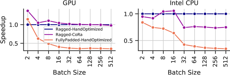
Figure 9: Performance comparison of CoRa’s vgemm and hand-optimized implementations of vgemm and fully padded gemm.

Triangular Matrix Multiplication: A triangular matrix, i.e. a matrix where all the elements above (or below) the diagonal are zero, can be thought of as a ragged tensor because all non-zero elements in a row are densely packed and their number per row is a function of the row index. Operations on triangular matrices can, thus, be effectively expressed and optimized using CoRa. In this section, we evaluate CoRa on the trmm operator wherein we multiply a square lower triangular matrix with a square dense matrix, on the Nvidia GPU. We compare against cuBLAS’s trmm and fully padded gemm implementations. In trmm, the reduction loop is a vloop. In order to efficiently handle the last few iterations of this loop after tiling, we use operation splitting (§4). Further, the raggedness in this loop leads to imbalanced load across the GPU thread blocks. We use thread remapping (§4.1) to schedule thread blocks with the most amount of work first, leading to more balanced load.

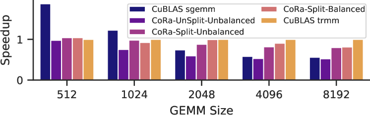
Figure 10: CoRa’s trmm performance compared against cuBLAS’s hand-optimized trmm and fully-padded gemm implementations.

Fig. 10 shows the performance of the aforementioned cuBLAS implementations and three implementations in CoRa—CoRa-unsplit-unbalanced, CoRa-split-unbalanced and CoRa-split-balanced—which progressively employ operation splitting and thread remapping, starting with neither. We see the trmm implementations—both cuBLAS’s and CoRa’s—are beneficial as compared to cuBLAS’s dense sgemm operator only for larger matrices. In all cases, however, the CoRa-split-balanced implementation performs within 81.3% of cuBLAS’s hand-optimized trmm implementation. Operation splitting leads to a significant increase in performance by allowing CoRa to elide conditional checks in the main body of the computation. Further, a better load distribution with thread remapping also helps CoRa achieve performance close to cuBLAS.

Table 3: Datasets used in our evaluation

Dataset (Short name, if any)	Min. / Mean / Max. SeqLength
RACE race	80 / 364 / 512
English Wikipedia with SeqLen 512 (Wiki512)	12 / 371 / 512
SQuAD v2.0 squadv2 (SQuAD)	39 / 192 / 384
English Wikipedia with SeqLen 128 (Wiki128)	14 / 117 / 128
MNLI mnli	9 / 43 / 128
XNLI xnli	9 / 70 / 128
MRPC mrpc	21 / 59 / 102
CoLA cola	6 / 13 / 37

7.2 The Transformer Model

We now move on to look at how CoRa performs on various modules of the transformer model. We mainly focus on the GPU backend as it is more commonly used for these models. We use a 6 layer model with a hidden dimension of 512 and 8 attention heads each of size 64. The encoder layer contains two feed-forward layers, the inner one of which has a dimension of 2048. These are the same hyperparameters used in the base model evaluated in transformer. We use sequence lengths from some commonly used NLP datasets listed in Table 3. We focus on larger batch sizes (32, 64 and 128) because, as we saw in Fig. 2, there is lesser opportunity to exploit raggedness for smaller batch sizes and hence other factors such as the quality of the schedules used in CoRa’s implementations play a big role. In this section, CoRa’s implementations use ragged tensor storage.

Table 4: Transformer encoder layer execution latencies (in ms) for CoRa, PyTorch and the two manually-optimized variants of FasterTransformer on the Nvidia GPU. CoRa’s execution latencies include prelude overheads assuming a 6 layer transformer encoder.

Dataset	Batch Size	PyTorch	FT	CoRa	FT-Eff
RACE	32	12.22	11.0	8.22	8.61
	64	24.46	21.88	15.91	16.75
	128	48.73	42.26	31.45	33.61
Wiki512	32	12.26	11.0	9.1	9.32
	64	24.52	22.12	17.4	17.85
	128	48.72	42.43	32.17	33.66
SQuAD	32	8.17	7.56	4.15	4.69
	64	16.9	15.63	7.78	9.2
	128	34.18	30.62	15.36	17.91
Wiki128	32	2.79	2.45	2.59	2.28
	64	5.12	4.61	4.72	4.35
	128	10.1	9.29	8.86	8.54
MNLI	32	2.22	2.04	1.11	1.03
	64	4.44	4.06	1.89	1.93
	128	9.53	8.86	3.53	3.78
XNLI	32	2.76	2.45	1.56	1.5
	64	5.13	4.62	2.94	2.86
	128	10.03	9.3	5.62	5.49
MRPC	32	1.85	1.73	1.32	1.27
	64	3.76	3.48	2.6	2.36
	128	7.42	6.89	4.55	4.55
CoLA	32	0.67	0.57	0.59	0.44
	64	1.02	0.93	0.77	0.63
	128	2.37	2.18	1.26	1.17

Transformer Encoder Layer: We first evaluate the forward pass latency of an encoder layer of the transformer model (Fig. 3). We compare CoRa’s performance with that of FasterTransformer and an implementation in PyTorch, a popular DL framework, with TorchScript TorchScript enabled. All the operators in the encoder layer except the ones in the SDPA sub-module process the hidden vectors associated with each word independently. Therefore, with manual effort, they can be implemented without any padding. The linear transformation operators Proj1, Proj2, FF1 and FF2 reduce to gemm operations in this case. FasterTransformer provides an option to perform this optimization, first introduced in EffectiveTransformers EffectiveTrans. We compare against FasterTransformer both with and without this optimization. We refer to these two implementations as FT-Eff and FT, respectively. In the CoRa implementation, this optimization is applied simply by loop fusion, analogous to the illustration in Fig. 6. In CoRa’s implementation however, we pad this fused loop so that its bound is a multiple of 64. In other words, we add a padding sequence to the batch to ensure that the sum of the sequence lengths is a multiple of 64. We refer to this kind of padding as bulk padding (Fig. 3). The relative amount of bulk padding added is usually quite low as the sum of sequence lengths in a batch is much higher.

Table 7.2 shows the forward execution latencies for the encoder layer for the aforementioned frameworks and datasets. The auxiliary data structures computed by CoRa’s prelude are shared across multiple layers of the model as the raggedness pattern stays the same across layers, depending only on the sequence lengths in the mini-batch. The execution times shown for CoRa include per-layer prelude overheads assuming a 6 layer model. We further look at these overheads in §7.4. As we can see, the CoRa implementation is competitive with the manually-optimized FT-Eff implementation for all datasets, even performing better in a few cases, and performs significantly better as compared to the fully-padded PyTorch and FT implementations. Fig. 11, which plots the overall performance of all these implementations for the batch sizes evaluated, makes this clear.

We now take a closer look at the FasterTransformer and CoRa implementations which are sketched in Fig. 3. The FT implementation is similar to the FT-Eff implementation except it uses full padding for all operations. The CoRa and FasterTransformer implementations differ in their operator fusion strategies. Therefore, the figure breaks the implementations down to the smallest sub-graphs that correspond to each other. Fig. 13 shows a breakdown of the execution times for these implementations for the RACE dataset and batch size 128 at the level of these sub-graphs. As Fig. 3 shows, the FT-Eff and CoRa implementations differ significantly with respect to padding only in the SDPA sub-module where the FT-Eff implementation employs full padding while the CoRa employs partial padding. We see, in Fig 13, that the CoRa implementation performs better than FasterTransformer for all the SDPA operators (QK^T, Softmax and AttnV) despite the fact that the latter is heavily hand optimized. This is because CoRa’s ability to handle raggedness enables it to perform less wasted computation. For the remaining operators where both the CoRa and FT-Eff implementations employ little to no padding, we see that the CoRa implementation is usually slower, but often close in performance to the FT-Eff implementation and significantly faster than the fully padded FT implementation. This is expected as FT-Eff calls into cuBLAS’s extensively optimized gemm kernels for the linear transformation operators and into hand-optimized kernels for the rest. CoRa’s performance drops slightly for datasets with smaller sequence lengths as well as for smaller batch sizes. As we discuss in §D.8, this performance difference can be reduced by further optimizing the schedules used for the projection and feed forward operators in CoRa’s implementation for smaller batch sizes and sequence lengths. Further, we also note that the overheads associated with the prelude code and partial padding (§7.4) play a larger role in these cases, further contributing to increased execution latencies.

FasterTransformer’s reliance on vendor libraries prevents it from fusing any of the gemm operations with surrounding elementwise operators, which CoRa can due to its compiler-based approach. Specifically CoRa can completely fuse all operators which add or remove padding in its implementation (as shown in Fig. 3). This is as opposed to the FT-Eff implementation, which cannot. Fusing these padding change operators leads to a significant drop in CoRa’s execution latency as seen in Fig. 12, which shows the execution latencies of the MHA module for the RACE dataset in CoRa with and without this fusion enabled.

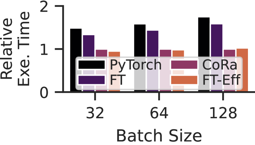
Figure 11: Relative execution times of the transformer encoder layer on the GPU.

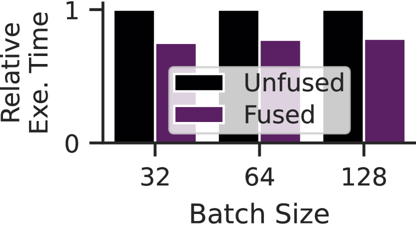
Figure 12: Benefits of padding change operator fusion for the MHA module.

Masked Scaled Dot-Product Attention: The decoder layer of a transformer uses a variant of MHA called masked MHA wherein the upper half of the attention matrix is masked for all attention heads during training. This masking only affects the SDPA module, the operators in which can now be seen as computing on a batch of lower triangular matrices. We saw in §7.1 that CoRa can effectively generate code for operations on triangular matrices. For batch size 128, an implementation of masked SDPA in CoRa which exploits this masking performs $1.56\times$ faster than an implementation which does not for the RACE dataset and $1.29\times$ for the MNLI dataset. The benefits are less pronounced for the MNLI dataset, which has smaller sequence lengths, as we pad vloops to be multiples of a constant regardless of the dataset. We provide more data and discussion on the implementation of masked SDPA in §LABEL:sec:ap_mmha_eval in the appendix.

Memory Consumption: We find that the use of ragged tensors leads to an overall $1.78\times$ drop in the size of the forward activations (computed analytically) of the encoder layer across all datasets at batch size 64 (more details in §LABEL:sec:ap_mem). The reduction, however, is not uniform across the datasets and those with higher mean sequence lengths, such as Wiki512 and Wiki128, see only small benefits. Forward activations often consume significant memory during training and ragged tensors can help alleviate memory bottlenecks along with other memory management techniques for training dtr; checkmate.

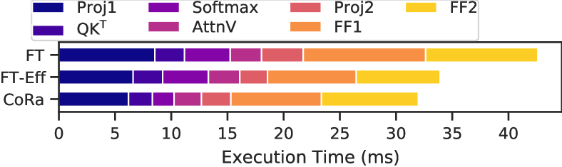
Figure 13: Breakdown of the encoder layer execution times for the RACE dataset at batch size 128. This data is obtained with profiling turned on and might deviate from Table 7.2.

Table 5: MHA execution latencies (in ms) on the 64-core ARM CPU for TensorFlow and CoRa.

Dataset	Batch Size 32			Batch Size 64			Batch Size 128
	TF	TF-UB	CoRa	TF	TF-UB	CoRa	TF	TF-UB	CoRa
RACE	55	46	44	111	88	85	209	156	168
Wiki512	53	53	47	106	96	91	205	172	176
SQuAD	35	27	20	68	49	39	137	79	76
Wiki128	11	11	9	19	18	17	34	33	33
MNLI	9	9	4	16	14	7	30	23	14
XNLI	11	11	6	18	18	11	34	28	22
MRPC	9	8	5	14	14	10	26	23	18
CoLA	5	4	2	6	6	3	9	8	5

MHA Evaluation on ARM CPU: Table 7.2 shows the execution latencies of MHA implementations in TensorFlow and CoRa on the 64-core ARM CPU. We evaluate against two execution configurations of TensorFlow—TF, where the entire mini-batch is executed at once and TF-UB, where the mini-batch is executed as a series of smaller micro-batches, which enables execution with lower padding. Across the datasets and batch sizes evaluated, we see that CoRa’s implementation is overall $1.57\times$ faster than TF and $1.37\times$ faster than TF-UB. In this case, too, CoRa’s ability to save on wasted computation due to padding leads to significant performance gains over a popular DL framework. §D.8 of the appendix more extensively compares the performance of TensorFlow and PyTorch against CoRa on both the 8- and 64-core ARM CPUs.

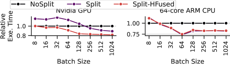
Figure 14: Benefits of operator splitting and hfusion. Note that the y-axis does not start at 0.

7.3 Operation Splitting and Horizontal Fusion

We now evaluate operator splitting and hfusion on the AttnV operator, which is an instance of the vgemm problem. AttnV has two vloops, one of which is a reduction loop. We apply the optimizations to the non-reduction vloop allowing us to use a larger tile size (we use 64) without padding the vloop bound to be a multiple of this tile size. This especially benefits datasets with sequence lengths comparable to the tile size, such as MNLI. For this dataset, Fig. 14 shows the relative execution times of three CoRa implementations of AttnV—NoSplit, Split and Split-HFused—in which we progressively perform the two optimizations, on the Nvidia GPU and 64-core ARM CPU backends. On the GPU, operation splitting causes a slowdown despite lower wasted computation as it reduces parallelism, which is restored by hfusion. This is more apparent at lower batch sizes when the amount of parallelism is lower. The effects of reduced parallelism due to operation splitting are less apparent on the CPU as it exposes lower levels of hardware parallelism. The lower levels of CPU parallelism also mean that hfusion has no benefit in this case. We also evaluate these optimizations on the QK^T operator in §LABEL:sec:ap_bp in the appendix.

7.4 Overheads in CoRa

Let us now look at the sources of overheads in CoRa—the prelude code, the wasted computation due to partial padding and auxiliary data structure accesses in the generated code.

Prelude Overheads: The prelude code constructs the required auxiliary data structures (§5) and copies them to the accelerator’s memory if needed. The table below lists the execution time (in ms) and memory (in kB) required for these tasks for a 6-layer transformer encoder on the GPU backend. It also shows the overheads associated with the storage lowering scheme used in past work we discussed in §5.3 (referred to as Sparse Storage in the table). As compared to this scheme, we see that CoRa’s specialized lowering scheme significantly reduces the resources required to compute the data structures associated with tensor storage. The overheads associated with loop fusion are higher than those associated with storage as we need to compute and store the relationship between all values of the fused and unfused loop iteration variables (§5.1). Copying the generated data structures to the GPU’s memory is, however, the major source of the overhead. Overall, the overheads range from 0.7% (RACE dataset at batch size 128) to about 7% (CoLA dataset at batch size 32) of the total execution time of the encoder layer on the GPU. On the CPU, the overheads are a very small fraction of the execution times, because the execution times are much higher and because the memory copy costs are absent. We discuss some simple optimizations to reduce prelude overheads in §LABEL:sec:ap_cora_overheads of the appendix.

Prelude Overheads: As we discussed in §LABEL:sec:ap_impl, CoRa’s prototype allows us to generate code for operator kernels one at a time. For each kernel, CoRa generates all the prelude code required for its execution. Therefore, when these generated kernels are invoked to form a larger model graph, as in our implementation of the transformer encoder layer, there is a lot of redundant computation in the prelude code. This is because (i) each operator computes the auxiliary data structures needed for all of its input and output tensors, which leads to these data structures being generated twice for every tensor in the graph, and (ii) the vloops in the schedules for all operators except the QK^T and the AttnV operators in CoRa’s implementation of the layer are fused similarly and can reuse the same auxiliary data structures, which are also currently computed separately for every operator. Tables 7.2 and 7.2 compare, for a 6-layer transformer encoder, the execution time and memory consumption of the prelude code respectively, as present in CoRa’s current implementation (referred to as CoRa-Redundant in the table) with an optimized implementation (referred to as CoRa-Optimized) which has all of this redundant computation removed. We see that when appropriately reused, the time and memory resources required to compute the auxiliary data structures in the prelude are quite low as compared to the those required for the execution of the kernel computation.

Table 8: Prelude memory usage (in kB) for a 6-layer transformer encoder with and without redundant computation.

Dataset	Batch Size	CoRa-Redundant		CoRa-Optimized
		CoRa Storage	CoRa Loop Fusion	CoRa Storage	CoRa Loop Fusion
CoLA	32	2.93	32.15	1.2	5.27
CoLA	128	11.18	104.22	4.58	17.5
RACE	32	2.93	666.54	1.2	106.87
RACE	128	11.18	2609.58	4.58	418.06

Overheads Due to Partial Padding: In Fig. 22, we show the relative amount of computation (computed analytically as in Fig. 2) for the transformer encoder layer for all datasets at batch sizes 32 and 128 for three cases—the fully padded dense case, the actual computation as evaluated in §7 with partial padding, and the ideal case with no padding. We see that partial padding leads to a very small increase in the amount of computation (3.5% across datasets for batch size 32 and 2.3% for batch size 128). Because we generally pad individual sequence lengths or their sum (as part of bulk padding) so that the quantity is a constant multiple of a small quantity (such as 32, or 64), the relative amount of padding added is higher for smaller batch sizes and datasets with smaller sequence lengths. Even in these cases, however, the added padding is much lower as compared to the benefits obtained with the use of ragged tensors. Further we note that the amount of padding added is a scheduling and optimization decision and can be changed if needed.

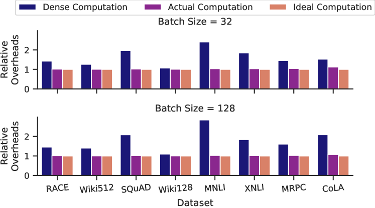
Figure 22: Overheads due to partial padding.

Ragged Tensor Overheads and Load Hoisting: We now take a closer look at the effects of auxiliary data structure accesses on the performance of CoRa-generated code. These data structure accesses arise in the generated code, as we have seen, due to the use of vloop fusion and ragged tensor storage. We focus on the five operators that make up the MHA module here. We measure the execution times of four implementations of each operator. The Dense implementation does not use ragged tensor storage or ragged computations. The +vloops implementation uses ragged computations, but the tensors are stored with full padding in a dense fashion. The +vdims implementation uses both ragged computations as well as ragged tensor storage. The +LoadHoist implementation is same as +vdims but hoists accesses to the auxiliary data structures out of loops as much as possible. In order to ensure that we perform the same amount of computation in all cases, we use a synthetic dataset where all sequences have the same length (512). The relative performance of these implementations for the operators on the Nvidia GPU is shown in Fig. 23. Apart from the overheads due to indirect memory accesses, the use of vloops and/or vdims also lead to overheads associated with the prelude code. In order to focus on the former overheads, however, we exclude prelude costs in the figure.

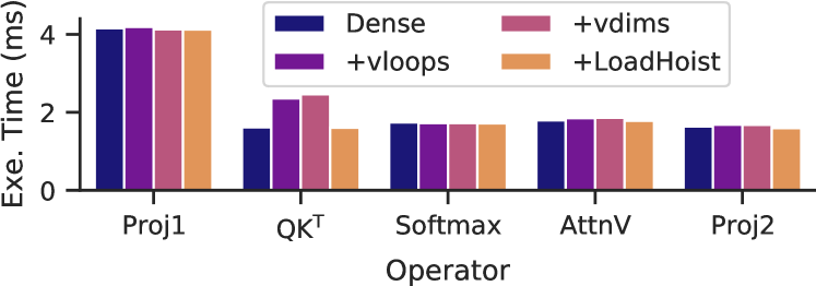
Figure 23: Overheads of using ragged computations and ragged tensor storage, and the benefits of load hoisting, measured for a synthetic dataset where all sequence lengths are 512. The batch size used is 64.

As the figure shows, the use of vloops and vdims leads to a slight slowdown for the Proj1, Softmax, Attnv and Proj2 operators. The slowdown is significant, however, for the QK^T operator, which has two vloops in its loop nest. As part of scheduling, we fuse both these vloops as well as the loop that the vloop bounds depend on (i.e. the loop that iterates over the mini-batch), leading to complex auxiliary data structure accesses. We believe that the CUDA compiler is unable to effectively hoist these accesses in this case. CoRa however has more knowledge about these accesses and can hoist them to recover the lost performance.

D.8 Discussion on Transformer Layer Evaluation

In this section, we provide further analysis of our evaluation of the transformer encoder layer on the Nvidia GPU and ARM CPU backends. We break down the execution time of the encoder layer for a few cases. As in Fig. 13, these per-operator execution times are obtained under profiling and might deviate slightly from the data in Tables 7.2 and 7.2.

Nvidia GPU Backend: Table 10 provides the raw data for the breakdown of the execution times for the RACE dataset at batch size 128 of the transformer encoder layer shown in Fig. 13 in the main text. Apart from improvements in the QK^T and AttnV operators discussed in §7.2, we note that CoRa’s implementation is significantly faster for the Softmax operator as compared to the FasterTransformer implementations. While we perform less computation on this operator as compared to the fully padded implementation in FasterTransformer, part of CoRa’s performance benefits also stem from a better schedule. Specifically, the FasterTransformer implementation performs parallel reductions across GPU thread blocks. This leads to a significant number of barriers at the thread block-level which have execution overheads. Further, the FasterTransformer implementation uses conditional checks to ensure that it never accesses attention scores for the added padding. In CoRa we use warp-wide parallel reductions which are much cheaper due to their lower synchronization costs but also provide a lower amount of parallelism. We, therefore, only partially parallelize the reductions and compensate with the high parallelism available in the other loops of the operator. Further, this means that we do not have to additionally employ conditional checks to avoid accessing invalid data (that is part of the partial padding we add).

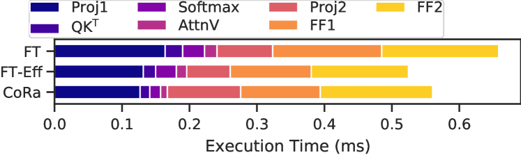
Figure 24: Breakdown of execution times of the encoder layer for the CoLA dataset at batch size 32 on the GPU.

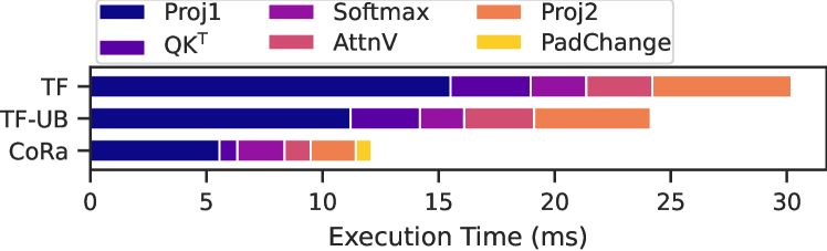
(a) MNLI dataset at batch size 128.

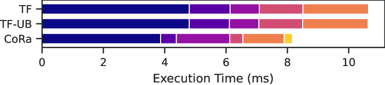
(b) Wiki128 dataset at batch size 32.

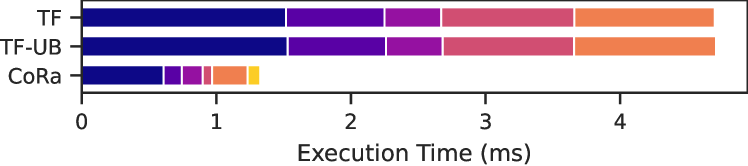
(c) CoLA dataset at batch size 32.

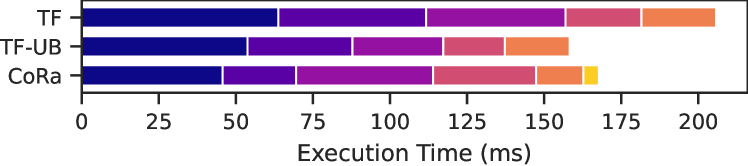
(d) RACE dataset at batch size 128.

Figure 25: Breakdown of execution times of the MHA module for four cases on the 64-core ARM CPU backend.

We now look at the execution time breakdown for the CoLA dataset at batch size 32 on the Nvidia GPU shown in Fig. 24. We see that CoRa performs slightly worse than FT-Eff for this case. Most of CoRa’s slowdown stems from worse performance on the linear transformation operators Proj2, FF1 and FF2. CoRa performs slightly better than FT-Eff for the Proj1 operator, which is also a linear transformation operator. From this data, we conclude that CoRa’s schedules for the Proj2, FF1 and FF2 operators can be improved to close this performance gap. We note that, even in this case, CoRa performs much better on the SDPA module (the QK^T, Softmax and AttnV operators) as compared to FasterTransformer.

ARM CPU Backends: In §7.2, we saw how CoRa performs better than TensorFlow for the MHA module on the 8- and 64-core ARM CPUs. In this section, we discuss these implementations in more detail and provide more extensive evaluation.

Table 9: MHA execution latencies (in ms) on 8- and 64-core ARM CPUs. uBS stands for the optimal micro-batch size.

Micro-Batching for PyTorch and TensorFlow: We saw, in Fig 2, that the amount of padding and wasted computation increases with the batch size. On devices that expose low levels of parallelism such as CPUs, it is therefore possible to trade-off batch parallelism for reduced padding, and therefore reduced wasted computation, for frameworks such as PyTorch and TensorFlow. In effect, this amounts to executing a mini-batch sorted by sequence lengths as a series of smaller micro-batches. Overall, this reduces the amount of padding needed as each micro-batch is only padded to the length of the longest sequence in that micro-batch, rather than the entire mini-batch as illustrated in Fig. 26. We search over micro-batch sizes that are powers of 2 starting from the lowest micro-batch size of 2. In Table D.8, we provide the execution latencies as well as the optimal micro-batch sizes for PyTorch and TensorFlow (these configurations is referred to as PT-UB and TF-UB respectively) for an 8-core as well as a 64-core ARM CPU. For reference, we also provide the latencies corresponding to naive executions of PyTorch and TensorFlow (referred to as PT and TF respectively) where the micro-batch size is equal to the mini-batch size.

Figure 26: Comparison of vanilla and micro-batched execution for PyTorch and TensorFlow.

CoRa’s MHA Implementation: As in CoRa’s vgemm implementation on the Intel CPU backend, we offload the computation of the dense inner tiles of the Proj1 and Proj2 operators in CoRa’s MHA implementation on the ARM backends to gemm calls in the OpenBLAS openblas library. Due to limitations of our prototype implementation, however, offloading the computation this way means that we cannot fuse the padding change operators with other computational operators in this case. We see in Fig. 25, however, that these pad fusion operators are relatively cheap to perform on the CPU backend.

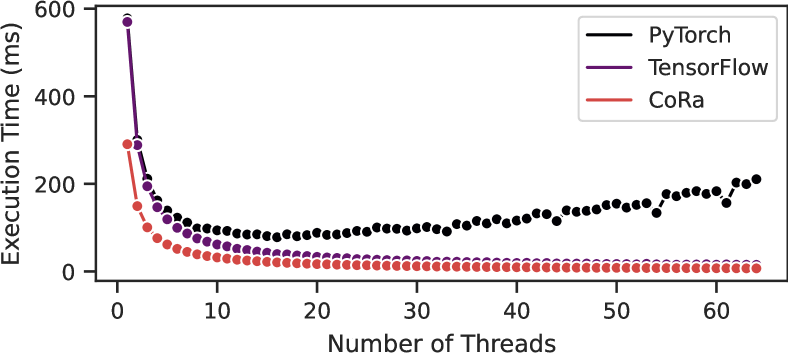
Figure 27: Execution latencies of PT, TF and CoRa as the number of threads is increased for the MNLI dataset at a batch size of 64. These measurements were performed on the 64-core CPU by changing the number of threads launched by OpenMP. Due to this, the measurements may not exactly be equal to the ones in Table D.8.

Overall Performance Comparison: Table D.8 shows the inference latencies for the PyTorch, TensorFlow and CoRa implementations of the MHA module on the 8- and 64-core ARM CPUs. We saw that TF-UB trades-off parallelism for reduced wasted computation. It, therefore, performs the best when there is high parallelism in the workload (i.e. for datasets with longer sequence lengths at higher batch sizes) and it performs the worst when the workload has low parallelism (i.e. for datasets with shorter sequences at lower batch sizes). This is because in the presence of high parallelism in the workload, TF-UB can reduce the micro-batch size much more (leading to much lower wasted padding) as compared to the case of a workload with low parallelism. This is seen reflected in the optimal micro-batch sizes shown in Table D.8. TF-UB also performs better on the 8-core CPU which exposes lower parallelism as compared to the 64-core CPUs. This is again reflected in the optimal micro-batch sizes which are generally higher (leading to higher padding) on the 64-core CPU as compared the 8-core CPU. Overall, we see that TF-UB and CoRa perform similarly on the 8-core ARM CPU, while CoRa outperforms TF-UB by about 1.37$\times$ as the hardware parallelism increases on the 64-core CPU. In both the cases, CoRa performs significantly better than the TF configuration of executing TensorFlow.

On the 8-core CPU, PyTorch in the PT-UB configuration performs better than both TF-UB and CoRa for datasets with higher sequence lengths. Similar to TF-UB, PT-UB can more effectively trade-off batch parallelism in these cases due to the high parallelism. Overall, across all the datasets and batch sizes evaluated, CoRa and PT-UB perform similarly, while TF-UB is about 6% slower than both on the 8-core CPU. We find that on the 64-core CPU, however, PyTorch’s performance does not scale well with the number of cores (this is apparent in Fig. 27) as compared to TensorFlow and CoRa. Therefore, below, we only consider TensorFlow for further analysis.

Per-Operator Execution Time Breakdown: Let us now look more closely at the execution times of the TensorFlow and CoRa implementations. Fig. 25 provides a breakdown of the execution times for four cases: (1) the MNLI dataset at a batch size of 128 and the Wiki128 dataset at a batch size of 32, which have the most and the least potential for savings on wasted computation due to padding as Fig. 2 shows, and (2) the RACE dataset at a batch size of 128 and the CoLA dataset at a batch size of 32, which represent the best and worst cases for the TF-UB configuration.

TF-UB and TF perform similarly for the CoLA dataset at batch size 32, as that represents the worst case for TF-UB, and on the Wiki128 dataset at batch size 128 as there is little potential for computational savings due to reduction in padding for that case. In the remaining two cases, TF-UB performs better than TF as expected. For the RACE dataset at batch size 128, which represents the best case for TF-UB, TF-UB performs slightly better than CoRa. In cases where CoRa performs better than TensorFlow, we find that a lot of the reduction in CoRa’s absolute execution time stems from computational savings in the Proj1 and Proj2 two operators, which consume a significant portion of the execution time. The QK^T and AttnV operators, however, show a higher relative reduction in execution time as they are quadratically proportional to the sequence lengths as opposed to Proj1 and Proj2 which are linearly proportional to sequence lengths. This difference in proportionality is also reflected in the data for the Wiki128 dataset. TensorFlow generally does well on the Softmax operator, performing better than CoRa for the RACE and Wiki128 datasets. We believe this is due to better optimized implementations and that this gap can be reduced with more time spent optimizing CoRa’s implementation of the operator.

Table 10: Breakdown of the encoder layer execution time for FasterTransformer and CoRa on the Nvidia GPU backend for the RACE dataset at batch size 128. Per-layer prelude code overheads are included in these latencies for CoRa. Both FasterTransformer and CoRa implementations normally execute CUDA kernels asynchronously. For the purposes of profiling (i.e., this table only), these calls were made synchronous, which can lead to slower execution. We also show the end-to-end execution times under profiling for reference.

Op sub-graphs	FT Ops	FT	FT-Eff	CoRa	CoRa Ops
Proj1	QKV Proj. MM	7.16	5.4	6.2	QKV Proj.
	QKV Bias + AddPad	1.39	1.21
QKT	QKT	2.65	2.64	2.12	AddPad + QKT
Softmax	Softmax	4.08	4.08	1.93	ChangePad + Softmax + ChangePad
AttnV	AttnV	2.78	2.79	2.44	AttnV
Proj2	Transpose + RemovePad	0.78	0.29
	Linear Proj. MM	2.42	1.82	2.31	RemovePad + Linear Proj. MM + Bias + ResidualAdd
	Linear Proj. Bias + ResidualAdd + LayerNorm	0.52	0.38	0.31	LayerNorm
FF1	FF1 MM	9.52	6.92	8.06	FF1 MM + Bias + Activation
	FF1 Bias + Activation	1.38	0.98
FF2	FF2 MM	9.47	7.1	8.33	FF2 MM + Bias + ResidualAdd
	FF2 Bias + ResidualAdd + LayerNorm	0.53	0.38	0.31	LayerNorm
	Total Execution Time	42.82	34.12	31.99	Total Execution Time

Appendix E Artifact Appendix

E.1 Abstract

This appendix describes how to reproduce the results described above in §7 and §LABEL:sec:ap_eval. The experiments in the paper evaluate CoRa on an Nvidia V100 GPU, an 8-core, 16-thread Intel CascadeLake CPU, an 8-core ARM Neoverse N1 CPU and a 64-core ARM Neoverse N1 CPU. Below, we provide instructions to set up and execute CoRa as well as other frameworks used in the evaluation on each of these platforms. As we start with publicly available Docker containers in all cases, only a few GPU-related dependencies (such as cuDNN) as well as CoRa’s dependencies (such as the Z3 SMT solver, LLVM and OpenBLAS) need to be installed. We provide instructions for each of these. In each case, 100 GB of disk space should be more than enough for the evaluation.

E.2 Artifact check-list (meta-information)

• Compilation: We reply on the publicly available compilers nvcc (the CUDA compiler to compile CUDA code generated by CoRa), gcc (to build CoRa and other dependencies) and LLVM (to facilitate CoRa’s code generation for CPUs).

• Data set: We use sequence lengths for 8 different commonly used NLP datasets, all of which are included in the repositories described below.

• Run-time environment: The artifact has been tested on Ubuntu 20.04 and with the following versions of different dependencies.

• Hardware: We use an Nvidia V100 GPU, an 8-core, 16-thread Intel CascadeLake CPU, an 8-core ARM Neoverse N1 CPU and a 64-core ARM Neoverse N1 CPU for our evaluation.

• Metrics: We use execution time as the primary execution metric of evaluation.

• Output: We generate CSV files, and also provide Python scripts to generate plots from this raw data.

• Experiments: Python/bash scripts are provided to replicate the results.

• Disk space required: 100 GB on each backend.

• Time needed to prepare workflow: A few hours on each backend.

• Time needed to complete experiments: Running all experiments on a backend takes several hours. The experiments on the ARM CPUs are particularly slow, taking 2-3 days to complete.

• Public availability: Yes, in the form of GitHub repositories (linked later) as well as on Zenodo (https://doi.org/10.5281/zenodo.6326455).

E.3 Description

E.3.1 How delivered

Source code in the form of Github repositories and archived on Zenodo.

E.3.2 Hardware dependencies

We use an Nvidia V100 GPU, an 8-core, 16-thread Intel CascadeLake CPU, an 8-core ARM Neoverse N1 CPU and a 64-core ARM Neoverse N1 CPU for our evaluation.

E.3.3 Software dependencies

GPU: Below, we describe the environment we use across the different hardware backends we evaluate CoRa on. On all of the backends, we use Ubuntu 20.04. Some of the frameworks below are already installed as part of the Docker images we start with (described below), while some need to be manually or installed. This is described below in §E.4.

Dependencies Common across Backends: CoRa requires the following frameworks on all platforms: Z3 4.8.8, LLVM 9.0.0, cmake $\geq$ 3.5 and g++ $\geq$ 5.0.

Nvidia GPU: CUDA 11.1 (V11.1.105), cuDNN 8.2.1, PyTorch 1.9.0+cu111, FasterTransformer (modified on top of FasterTransformer v4.0 (commit dd4c071) and provided as part of the cora_benchmarks repository). Make sure that nvcc is on the PATH.

ARM CPUs: OpenBLAS 0.3.10, PyTorch 1.10.0 with ARM Compute Library 21.12, TensorFlow 2.6.0 with ARM Compute Library 21.09.

Intel CPU: Intel oneAPI MKL v2021.3.

E.3.4 Data sets

All datasets are included in the cora_benchmarks repository.

E.4 Installation

Refer to the file ae_appendix_supplement.pdf at the root of the cora repository.

E.5 Experiment workflow

As we saw above, CoRa is a tensor compiler. It takes as input a description of a tensor operator and generates LLVM or CUDA code for the kernel depending on whether the target is a CPU or a GPU. For evaluating individual kernels, such as trmm, vgemm or any of the nine kernels that make up the transformer layer (illustrated in Figure 3 of the paper), merely executing the python script implementing the kernel will compile the kernel, generate the code and execute it. For evaluating the entire transformer layer, or parts of it (such the self-attention or the MHA modules), we separate the steps of code generation and execution (§LABEL:sec:ap_impl). We first generate compiled code for each of the operators in the form of shared libraries, which are then loaded and executed to form the layer to benchmark layer performance. The scripts provided automate all of these steps.

E.6 Evaluation Notes and Instructions

Refer to the file ae_appendix_supplement.pdf at the root of the cora repository for instructions on how to perform the evaluation on the platforms referred to in the paper.

E.7 Experiment customization

1. GPU Evaluation: The GPU evaluation has been tested on Nvidia GPUs with compute capability 70. While the evaluation may run on other Nvidia GPUs as well, we have not yet tested it thoroughly. CoRa can currently only support Nvidia GPUs as it only supports the generation of CUDA code.

2. CPU Evaluation: The Intel and the ARM CPU evaluation should work for other CPUs beyond the CascadeLake and the Neoverse N1 CPUs we have tested it on. However, given that our schedules have been tuned for these CPUs, the performance might not be optimal. Further, when running on other CPUs, the LLVM target triple would need to be changed (in the file cora_benchmarks/scripts/common.py on line 10). The number of threads would also be need to be changed for PyTorch evaluation in the files cora_benchmarks/bert_layer/pytorch/layer_cpu_micro_batch.py and cora_benchmarks/bert_layer/pytorch/layer_cpu.py on the appropriate branch of the cora_benchmarks repository.