Cutting Voxel Projector a New Approach to Construct 3D Cone Beam CT Operator

Abstract

In this paper, we introduce a new class of projectors for 3D cone beam tomographic reconstruction. We find analytical formulas for the relationship between the voxel volume projected onto a given detector pixel and its contribution to the extinction value detected on that pixel. Using this approach, we construct a near-exact projector and backprojector that can be used especially for algebraic reconstruction techniques. We have implemented this cutting voxel projector and a less accurate, speed-optimized version of it together with two established projectors, a ray tracing projector based on Siddon’s algorithm and a TT footprint projector. We show that the cutting voxel projector achieves, especially for large cone beam angles, noticeably higher accuracy than the TT projector. Moreover, our implementation of the relaxed version of the cutting voxel projector is significantly faster than current footprint projector implementations. We further show that Siddon’s algorithm with comparable accuracy would be much slower than the cutting voxel projector. All algorithms are implemented within an open source framework for algebraic reconstruction in OpenCL 1.2 and C++ and are optimized for GPU computation. They are published as open-source software under the GNU GPL 3 license, see https://github.com/kulvait/KCT_cbct.

I Introduction

Tomographic reconstruction is a problem of inverting Radon transformation in 2D or 3D in order to recover unknown attenuation $\mu(.)$ from the set of line integrals that represents measured data. Analytical methods are based on a direct expression for the inverse or an approximation of it, see [1, 2, 3]. Analytical formulas do not include discretization, which must be considered separately.

Algebraic methods, on the other hand, rely on the formulation of a projection operator that models X-ray absorption and accounts for discretization. The CT operator $\mathbf{A}\in\mathbb{R}^{m\times n}$ directly describes the relationship between the voxel attenuation values in the imaged sample $\mathbf{x}\in\mathbb{R}^{n}$ and the pixel extinction values on the detector $\mathbf{b}\in\mathbb{R}^{m}$ so that

$$\mathbf{A}\mathbf{x}=\mathbf{b}.$$ (1)

Algebraic methods aim to compute the vector $\mathbf{x}_{min}$ that minimizes certain functional, such as the squared residual error for given projection data $\boldsymbol{b}$, using an iterative process, see [4, 5]. The possibility to choose the proper search space for the solution, together with the variability of the form of the functional to minimize makes these methods a versatile tool for CT reconstruction. They are suitable for applications such as limited-angle reconstruction, a priori knowledge problems or time-dependent reconstruction of contrast agent dynamics in perfusion imaging, see for example [6].

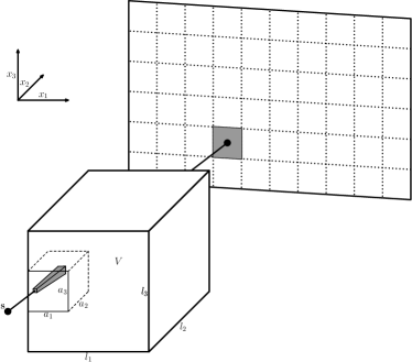
Figure 1: Cutting voxel projector estimates detected extinction at particular pixel based on the volume of the intersection of each voxel with all possible rays to the pixel.

Iterative methods require efficient and accurate evaluation of the actions of projection and backprojection operators. The projection operator acts on volume data $\mathbf{x}_{\mathrm{IN}}\in\mathbb{R}^{n}$ and returns the projection vector $\mathbf{b}_{\mathrm{OUT}}\in\mathbb{R}^{m}$ such that $\mathbf{b}_{\mathrm{OUT}}=\mathbf{A}\mathbf{x}_{\mathrm{IN}}$. The backprojection operator acts on projection vector $\mathbf{b}_{\mathrm{IN}}\in\mathbb{R}^{n}$ and returns the volume data $\mathbf{x}_{\mathrm{OUT}}\in\mathbb{R}^{n}$ such that $\mathbf{x}_{\mathrm{OUT}}=\mathbf{A}^{\top}\mathbf{b}_{\mathrm{IN}}$. Because the I/O latencies of data storage devices are high, it is prohibitive for typical CT systems to store the matrix $\mathbf{A}$ on disk and perform these matrix multiplications directly. Computing the projection and backprojection operators on the fly on current GPUs is typically orders of magnitude faster than working with the $\mathbf{A}$ matrix stored on disk. Therefore, there is a demand for fast and accurate projection and backprojection operators.

Ray casting/tracing projectors are well established not only in the context of CT imaging, but also in the context of computer graphics, see [7, 8, 9]. They track the ray cast from the source to the detector and add the extinction values along the way to form the product of the $\mathbf{A}$ row with given vector $\mathbf{x}_{\mathrm{IN}}$. Outer loop of these projectors is over the detector pixels, so they are scanning the matrix $\mathbf{A}$ row by row. Their accuracy is strongly dependent on the number of rays cast. Backprojection is typically slower than projection and, in addition, it is unable to capture the underlying physical process well, resulting in a strong geometric artefacts in reconstructions.

Footprint projectors on the other hand try to estimate for each voxel and position on the detector the length of the intersection of the voxel with the ray to that position. Their outermost loop is over voxels, so that they scan the matrix $\mathbf{A}$ column by column. Current implementations rely on the assumption that footprints can be approximated in each detector direction by very simple functions, for example by constants with a small support, see [10], or by constants in the middle with linearly decaying tails on each side, so-called trapezoidal functions. Separable footprint projectors approximate blur on the detector due to a given voxel by product of two such functions, each for one detector dimension, see [11]. They extend the work of [10] and are considered state of the art CT projectors. The inaccuracies of this class of projectors are due to the fact that the actual footprints are generally not separable and thus do not satisfy assumptions about the shape of the footprint functions.

In this paper, we construct a projector that directly describes the voxel pixel correspondence by computing integrals over the volumes of voxel cuts projected onto a given pixel instead of averaging line integrals over rays passing through the voxels, see Figure 1. In order to accurately compute the projection of a given voxel onto a given pixel, we need to reformulate the problem using integral calculus to find the correspondence between the integrals over all rays passing through the voxel and the integrals over the voxel cut volume. This approach eliminates the need to cast a high number of rays towards a given pixel to increase accuracy, and also overcomes assumptions about the shapes of the footprints.

II Problem formulation

In this section we derive fast, almost exact projector for 3D cone beam geometry. We use linear Lambert-Beer law to compute pixel signal based on the known function $\mu:\mathbb{R}^{3}\to\mathbb{R}^{+}_{0}$ that represents the attenuation. We emphasize that instead of direct integration of the attenuation over the rays to the detector we find a mathematical transformation to integrate attenuation over the subvolumes of voxels projected to given pixel.

II-A Geometry discretization

Throughout the paper, we will use the following standard assumptions about the discretized problem. Let’s the X-ray source, object to be scanned and the detector be located in the Euclidean space $\mathbb{R}^{3}$. The X-ray source at given time $t$ has coordinates $\mathbf{s}=(s_{1},s_{2},s_{3})$. The object to be scanned lies inside a rectangular box $V$ centered at $(0,0,0)$ with the edge lengths $(l_{1},l_{2},l_{3})\in\mathbb{R}_{+}^{3}$. Box $V$ represents the volume to be projected

$$V=\{\mathbf{x}\in\mathbb{R}^{3}:|x_{1}|<\frac{l_{1}}{2},|x_{2}|<\frac{l_{2}}{2},|x_{3}|<\frac{l_{3}}{2}\}.$$

The discretization is given by the voxel sizes $(a_{1},a_{2},a_{3})\in\mathbb{R}_{+}^{3}$ and number of the voxels per edge $(N_{1},N_{2},N_{3})\in\mathbb{N}^{3}$. For the dimension compatibility it is required that $a_{\alpha}N_{\alpha}=l_{\alpha}$ for $\alpha\in\{1,2,3\}$. Let’s denote the center of the voxel $(0,0,0)$ by

$$\mathbf{x}^{(0,0,0)}=(\frac{-l_{1}+a_{1}}{2},\frac{-l_{2}+a_{2}}{2},\frac{-l_{3}+a_{3}}{2}).$$

The center of the general voxel $(i,j,k)$, $i\in\{0...N_{1}-1\}$, $j\in\{0...N_{2}-1\}$ and $k\in\{0...N_{3}-1\}$ is then

$$\mathbf{x}^{(i,j,k)}=\mathbf{x}^{(0,0,0)}+(ia_{1},ja_{2},ka_{3}),$$

and the volume of the voxel is given by

$$V^{(i,j,k)}=\{\mathbf{x}\in\mathbb{R}^{3}:|x_{\alpha}-x^{(i,j,k)}_{\alpha}|<\frac{a_{\alpha}}{2},\alpha\in\{1,2,3\}\}.$$

The attenuation $\mu:\mathbb{R}^{3}\to\mathbb{R}^{+}_{0}$ has a support on $V$ and is constant on each voxel so that

$$\forall\mathbf{x}\in V^{(i,j,k)}\quad\mu(\mathbf{x})=\mu^{i,j,k}.$$

II-B Detector discretization

In what follows, we consider flat panel detector with the rectangle shaped pixels without gaps. Detector surface is parametrized by means of two Euclidean coordinates $\chi=(\chi_{1},\chi_{2})\in\mathbb{R}^{2}$. These assumptions allow us to clearly explain main concepts, yet it is straightforward to relax them and consider curved detectors, differently shaped pixels and gaps between pixels. In the current implementation, to compute the cuts, we additionally assume that the $x_{3}$ axis of the global geometry is parallel to the $\chi_{2}$ axis of the detector, see Figure 3. However, this assumption is not essential to derive the main formula for the extinction of the cutting voxel projector in this chapter.

Let’s assume that $(M,N)\in\mathbb{N}^{2}$ are the counts of the pixels per edge and the spacing of pixels is given by $(b_{1},b_{2})\in\mathbb{R}_{+}^{2}$. The center of the pixel $(0,0)$ is $\mathbf{\chi}^{(0,0)}=(0,0)$. The center of the general pixel $(m,n)$, $m\in\{0...M-1\}$ and $n\in\{0...N-1\}$ is at

$$\mathbf{\chi}^{(m,n)}=\mathbf{\chi}^{(0,0)}+(mb_{1},nb_{2})$$ (2)

and the surface of the pixel is parametrized as

$$A^{(m,n)}=\{\mathbf{\chi}:|\chi_{\alpha}-\chi^{(m,n)}_{\alpha}|<\frac{b_{\alpha}}{2},\alpha\in\{1,2\}\}.$$ (3)

II-C Parametrization of the rays and attenuation model

Let’s fix the source and the detector position and introduce the spherical coordinate system $(r,\theta,\varphi)\in[0,\infty]\times[0,\pi/2]\times[0,2\pi)$ that originates in the source position and describes rays to the detector. The zenith denotes the direction with zero inclination $\theta=0$, which corresponds to the principal ray that is the ray orthogonal to the flat panel detector. The intersection of the detector with the principal ray is called the principal point $\mathbf{\chi}^{P}=(\chi_{1}^{P},\chi_{2}^{P})$. Rays with azimuth $\varphi=0$ are projected onto a semi-line on the detector starting at a principal point parallel to the $\chi_{1}$ axis.

For a given view, there is an exact correspondence between this local spherical coordinate system and the global coordinate system. We can introduce an auxiliary Euclidean system $(\tilde{x}_{1},\tilde{x}_{2},\tilde{x}_{3})$ centered at $\mathbf{s}$ and the transformation given by orthogonal $3\times 3$ matrix $Q$ such that

$$\tilde{\mathbf{x}}=Q(\mathbf{x}-\mathbf{s}).$$ (4)

The rotation $Q$ transforms the axes so that $x_{1}$ is parallel to the detector coordinate $\chi_{1}$, $x_{2}$ is parallel to $\chi_{2}$ and $x_{3}$ is in the direction of the normal from the source to the detector, see Figure 2. The system $(\tilde{x}_{1},\tilde{x}_{2},\tilde{x}_{3})$ then in turn induces local spherical coordinate system in a way that

$$r =\sqrt{\tilde{x}_{1}^{2}+\tilde{x}_{2}^{2}+\tilde{x}_{3}^{2}},$$ (5)

$$\theta =\arccos\frac{\tilde{x}_{3}}{\sqrt{\tilde{x}_{1}^{2}+\tilde{x}_{2}^{2}+\tilde{x}_{3}^{2}}},$$ (6)

$$\varphi =\operatorname{atan2}(\tilde{x}_{2},\tilde{x}_{1}).$$ (7)

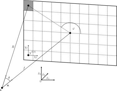
Figure 2: Auxiliary local Euclidean coordinates for a given view that induce a local spherical coordinate system. Coordinate $\theta$ is the cone angle.

The model given by Lambert-Beer law and the cone beam geometry maps the lines in $\mathbb{R}^{3}$ starting at the source position $\mathbf{s}$ to the integrals over the attenuation $\mu$ along these lines. The lines can be parametrized by polar and azimuthal angles in spherical coordinate system $[\theta,\varphi]\in[-\pi/2,\pi/2]\times[0,2\pi)$. Let’s $\mathbf{L}[\theta,\varphi]:\mathbb{R}\to\mathbb{R}^{3}$ define a isometric parametrization $\mathbf{L}[\theta,\varphi](q),q\in[0,\infty)$ of the ray in the direction $[\theta,\varphi]$ such that $\mathbf{L}[\theta,\varphi](0)=\mathbf{s}$.

We identify the coordinates $\chi=(\chi_{1},\chi_{2})\in\mathbb{R}^{2}$ with the parameters $\theta,\varphi$, which define the line line through the source $L[\theta,\varphi](.)$ that hits the detector at $(\chi_{1},\chi_{2})$. We consider $[\theta,\varphi]$ or $[\chi_{1},\chi_{2}]$ just two different parametrizations of the set of all lines passing through the $\mathbf{s}$. In the projective geometry such set is called projective plane or projective space of dimension two, see [12].

Consider the ray in the direction $[\theta,\varphi]$. According to Lambert-Beer law the X-ray intensity after passing the scanned object measured on the detector is

$$I(\theta,\varphi)=I_{0}(\theta,\varphi)\exp{\left(-\int\limits_{0}^{\infty}\!\mu(\mathbf{L}[\theta,\varphi](q))\,\mathrm{d}q\right)},$$ (8)

where $I_{0}(\theta,\varphi)$ is the blank scan intensity that would be measured at the same detector position without scanned object. The extinction is then defined as

$$E(\theta,\varphi)\stackrel{{\scriptstyle 1}}{{=}}\ln(I_{0}(\theta,\varphi))-\ln(I(\theta,\varphi))\stackrel{{\scriptstyle 2}}{{=}}\int\limits_{0}^{\infty}\!\mu(\mathbf{L}(\theta,\varphi,q))\,\mathrm{d}q.$$ (9)

II-D Per pixel extinction

When scanning the volume $V$, the CT scanner measures the intensities $I^{(m,n)}$ for each view and each pixel on the detector and and then calculates the extinction values $E^{(m,n)}$ based on the known per pixel intensities $I_{0}^{(m,n)}$ and the first relation in (9). The values of $E^{(m,n)}$ represent the input vector $\mathbf{b}$ of the reconstruction problem (1). In order to obtain specific values within the matrix $\mathbf{A}$, the so-called geometric factors, we need to determine the specific form of the second equation in (9) for the discretized extinction $E^{(m,n)}$.

A first order approximation of the relationship between voxel and pixel values is to cast rays towards the pixels and construct the CT operator as follows

$$E^{(m,n)}=\sum_{i,j,k}\mu^{i,j,k}|V^{(i,j,k)}\cap\mathbf{L}(\chi^{(m,n)},.))|,$$ (10)

where $|V^{(i,j,k)}\cap\mathbf{L}(\chi^{(m,n)},.))|$ is the length of the path of given ray through the given voxel. For computing these intersections, we utilize Siddon algorithm, see [7]. The problem with this approach is that the extinction value $E^{(m,n)}$ depends on the exact location on the pixel surface where the beam is cast. The solution is, for example, to create a grid of $K\times K$ equally spaced points on the pixel surface and average all extinction values in (10) with respect to the rays thrown towards the grid points. We will henceforth refer to the algorithm obtained in this way as SiddonK, i.e., for example, Siddon8 casts 64 rays towards each pixel.

To robustly estimate the extinction over pixels, we use the following formula using the integral over the pixel area, which can also be obtained as a limit process derived from the sum over grid points in the SiddonK algorithm if we send $K$ to infinity.

$$E^{(m,n)}=\frac{e^{(m,n)}}{a^{(m,n)}},$$ (11)

where

$$e^{(m,n)}=\int_{\chi\in A^{(m,n)}}\sum_{i,j,k}\mu^{i,j,k}\mathcal{D}(\chi,i,j,k)\,dS(\chi),$$ (12)

is the total extinction over the area of the pixel,

$$\mathcal{D}(\chi,i,j,k)=|V^{(i,j,k)}\cap\mathbf{L}(\chi,.))|$$ (13)

is the length of the path of the ray parametrized by $\chi$ through voxel $(i,j,k)$ and

$$a^{(m,n)}=\int_{\chi\in A^{(m,n)}}1\,dS(\chi).$$ (14)

The integrals (12) and (14) are over the parameterization $\,dS(\chi)$ of the infinitesimal detector surface at point $\chi$ in world coordinates, so that $a^{(m,n)}$ is the area of a given pixel.

Alternatively, we can transform the problem to the unit ball. As we noted $(\theta,\varphi)$ can be also understood as a discretization of unit ball centered at the source position $\mathbf{s}$. Therefore for given pixel we can integrate (9) along $(\theta,\varphi)$ that maps to a given pixel and divide by the surface of the unit ball that maps to that pixel. We have the formula

$$\bar{E}^{(m,n)}=\frac{\bar{e}^{(m,n)}}{\bar{a}^{(m,n)}},$$ (15)

where

$$\bar{e}^{(m,n)}=\int\limits_{(\theta,\varphi)\in A^{(m,n)}}\sum_{i,j,k}\mu^{i,j,k}\mathcal{D}(\theta,\varphi,i,j,k)\sin\theta\mathrm{d}\theta\mathrm{d}\varphi$$ (16)

is the total extinction over the area of the unit ball segment

$$\bar{a}^{(m,n)}=\int\limits_{(\theta,\varphi)\in A^{(m,n)}}\sin\theta d\,\theta d\,\varphi.$$ (17)

Here we utilize formula for the unit ball surface element being $dS=\sin\theta d\,\theta d\,\varphi$.

II-E Cutting voxel projector

To derive new strategy to compute (11) or (15), we transform integrals over the area of detector cells in (12) and (16) into the integrals over the volume of the voxels of the type

$$\int_{V}\mu(\mathbf{x})\,dx.$$ (18)

Using this approach, instead of averaging the ray path length over a voxel, we can then calculate the voxel volume projected onto a given pixel and derive the extinction increment from this value. We start by rewriting the integral (12) into the form

$$e^{(m,n)}=\sum_{i,j,k}\mu^{i,j,k}e_{i,j,k}^{(m,n)},$$ (19)

where

$$e_{i,j,k}^{(m,n)}=\int_{\chi\in A^{(m,n)}}|V^{(i,j,k)}\cap\mathbf{L}(\chi,.)|\,dS(\chi).$$ (20)

Let’s define an indicator function that tests if the line at the point given by the local spherical coordinates introduced in Figure 2, intersects the voxel

$$\mathbf{I}^{i,j,k}(r,\theta,\varphi)=\begin{cases}1\quad\mbox{if }\mathbf{L}(\theta,\varphi,r)\in V^{(i,j,k)}\\ 0\quad\mbox{elsewhere.}\end{cases}$$ (21)

Applying (21), we rewrite the length of the voxel ray intersection in (20) as

$$|V^{(i,j,k)}\cap\mathbf{L}(\chi,.)|=\int_{0}^{\infty}\mathbf{I}^{i,j,k}(r,\theta(\chi),\varphi(\chi))d\,r.$$ (22)

The surface element in spherical coordinates is $\mathrm{d}\tilde{S}(\chi)=R^{2}\sin{\theta}\,\mathrm{d}\theta\,\mathrm{d}\varphi$, where $R$ is the distance of a given pixel on the detector from the source. We assume that the pixel is small enough so that $R$ over its area can be approximated by a constant value, and also that the curvature of the spherical coordinates on its surface can be ignored so that the angle between the pixel and the element $\mathrm{d}\tilde{S}(\chi)$ is constant. The element $\mathrm{d}\tilde{S}(\chi)$ is perpendicular to the ray so that the angle of its normal with the normal to the pixel is $\theta$, the cone angle. The correction for integration over the surface element of a pixel is therefore of the form $\mathrm{d}\tilde{S}(\chi)=\cos{\theta}\,\mathrm{d}S(\chi)$. Combining this equality with (20) and (22) yields

$$e_{i,j,k}^{(m,n)}=\int\limits_{0}^{\infty}\!\int\limits_{\chi\in A^{(m,n)}}\mathbf{I}^{i,j,k}(r,\varphi(\chi),\theta(\chi)))R^{2}\frac{\sin{\theta}}{\cos{\theta}}\,d\theta\,d\varphi\,\mathrm{d}r.$$ (23)

Volume element in spherical coordinates has a form

$$dV=r^{2}\sin{\theta}\,d\theta\,d\varphi\,dr$$ (24)

so the integral (23) can be rewritten to the form

$$e_{i,j,k}^{(m,n)}=\int_{V^{(i,j,k)}_{(m,n)}}\frac{R^{2}}{r^{2}\cos{\theta}}\,dV,$$ (25)

where $V^{(i,j,k)}_{(m,n)}$ is a intersection of voxel $(i,j,k)$ with all rays to the pixel $(m,n)$. We assume that $\cos{\theta}$ and $R$ are constant on each detector pixel and approximate them by the value in its center. When $f$ is the distance from s to the detector, we have that

$$R\cos{\theta}=f,$$ (26)

which further simplifies (25) into the form

$$e_{i,j,k}^{(m,n)}=\frac{f^{2}}{\cos^{3}{\theta}}\int_{V^{(i,j,k)}_{(m,n)}}\frac{1}{r^{2}}\,\mathrm{d}V$$ (27)

and establishes the formula for the discrete extinction of the cutting voxel projector

$$E^{(m,n)}=\frac{f^{2}}{a^{(m,n)}\cos^{3}{\theta}}\sum_{i,j,k}\mu^{i,j,k}\int_{V^{(i,j,k)}_{(m,n)}}\frac{1}{r^{2}}d\,x.$$ (28)

For the geometry of the detector transformed to the surface of the unit sphere, we start from the integral (16). The derivation is easier because we do not have to correct for the angle mismatch of the infinitesimal element of the pixel surface and the infinitesimal element of the spherical coordinates as it is zero. The formula analogous to the integral (23) reads

$$\bar{e}_{i,j,k}^{(m,n)}=\int\limits_{0}^{\infty}\!\int\limits_{\chi\in A^{(m,n)}}\mathbf{I}^{i,j,k}(r,\varphi(\chi),\theta(\chi)))\sin{\theta}\,\mathrm{d}\theta\,\mathrm{d}\varphi\,\mathrm{d}r,$$ (29)

With the formula for the volume element in spherical coordinates $\mathrm{d}V=r^{2}\sin{\theta}\,\mathrm{d}\theta\,\mathrm{d}\varphi$ it might be concluded that

$$\bar{e}_{i,j,k}^{(m,n)}=\int_{V^{(i,j,k)}_{(m,n)}}\frac{1}{r^{2}}\,\mathrm{d}V.$$ (30)

For the computation of the area of the unit ball that gets projected to the given pixel in (17), we can utilize spherical trigonometry, see [13] and [14, p. 98-99]. For the area of the polygon on the unit sphere we have

$$\bar{a}^{(m,n)}=\alpha+\beta+\gamma+\delta-2\pi,$$ (31)

where $\alpha$, $\beta$, $\gamma$ and $\delta$ are sizes of the four polygon angles on that sphere. So let’s have unit vectors $\mathbf{t}_{0}^{(m,n)}$, $\mathbf{t}_{1}^{(m,n)}$, $\mathbf{t}_{2}^{(m,n)}$, $\mathbf{t}_{3}^{(m,n)}$ in the direction of the pixel corners ordered counter clock wise. After some manipulations we can conclude

$$\bar{a}^{(m,n)}=2\pi-\sum_{i=0}^{3}\arccos{\frac{(\mathbf{t}_{i}\times\mathbf{t}_{i+1})\cdot(\mathbf{t}_{i+1}\times\mathbf{t}_{i+2})}{|\mathbf{t}_{i}\times\mathbf{t}_{i+1}||\mathbf{t}_{i+1}\times\mathbf{t}_{i+2}|}}.$$ (32)

The equation (11) became

$$\bar{E}^{(m,n)}=\frac{1}{\bar{a}^{(m,n)}}\sum_{i,j,k}\mu^{i,j,k}\int_{V^{(i,j,k)}_{(m,n)}}\frac{1}{r^{2}}d\,x.$$ (33)

Equations (28) and (33) are general forms of discrete extinction for cutting voxel projector in flat panel geometry and in the geometry transformed to a unit sphere. Note that the two formulations (28) and (33) differ only in the form of the factor in the product for a given pixel. It is therefore possible to first calculate the sum of

$$S^{(m,n)}=\sum_{i,j,k}\mu^{i,j,k}\int_{V^{(i,j,k)}_{(m,n)}}\frac{1}{r^{2}}d\,x,$$ (34)

which is the same for both formulations and then rescale these sums at the pixel level according to the chosen formulation.

II-F Volume of the voxel cuts

To be able to use formulas (28) or (33) we have to be able to evaluate value $\bar{e}_{i,j,k}^{(m,n)}$ by means of the integral (30) for each pixel and voxel pair.

Here we assume that the voxel cuts are such small that $r^{2}$ is approximately constant for the whole volume $V^{(i,j,k)}_{(m,n)}$. We can estimate $r=r_{i,j,k}$ being the distance of the center of the given voxel to the source $s$ or more precisely $r=r_{i,j,k,m,n}$ being the distance of the center of mass of $V^{(i,j,k)}_{(m,n)}$ to the source. This assumption enables us to write (30) in the form

$$\bar{e}_{i,j,k}^{(m,n)}=\sum_{i,j,k}\frac{\mu^{i,j,k}}{r_{i,j,k,m,n}^{2}}|V^{(i,j,k)}_{(m,n)}|.$$ (35)

This concludes the theoretical derivation of the cutting voxel projector. In the next section, we present our current implementation and describe how the calculation of the volume of voxel cuts for each voxel pixel pair is handled in it.

III Implementation

The current cutting voxel projector implementation is part of a larger framework for CBCT reconstruction available at https://github.com/kulvait/kct_cbct developped by the first author. It is a set of tools written in C++ and OpenCL 1.2 optimized to run on GPU architectures with fast local memory. The software is released under the open source license GNU GPL3.

III-A Calculating voxel cuts

To simplify the calculation of the voxel cuts, we assume a geometric arrangement where the $\chi_{2}$ axis of the detector is parallel to the $x_{3}$ axis of world coordinates and by convention their directions are opposite, see Figure 3. This arrangement is used in most current CT trajectories, including the circular trajectory, and is also assumed by footprint projectors, see [11].

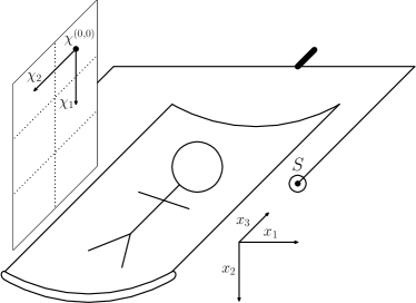
Figure 3: Geometric convention and simplification for the classical cone beam CT arrangement. The axis of rotation is parallel to the $x_{3}$ axis of world coordinates. In addition, the $x_{3}$ axis is parallel to the $\chi_{2}$ axis of the detector, but they have opposite orientations. The origin of the detector is placed in the center of the corner pixel. This arrangement is also assumed in the software.

Then, for any two points $x^{I}=(x_{1},x_{2},x_{3})$ and $x^{II}=(x_{1},x_{2},x_{3}^{\prime})$, which differ only in the value of the third world coordinate it holds that

$$\chi_{1}(x^{I})=\chi_{1}(x^{II}).$$ (36)

Therefore, the projection onto the $\chi_{1}$ is independent of the value of $x_{3}$. That means that the profiles of the cuts through a given voxel in the $x_{1}x_{2}$ plane will be the same for all $x_{3}$ coordinates of given voxel and moreover they will be the same for all the voxels with the same fixed $i$ and $j$ indices $V^{i,j,.}$.

Based on this observation, we first find for each voxel $V^{i,j,k}$ and coordinate $n$ on the detector the polygons $H^{i,j}_{n}$ into which the base of the voxel parallel with the $x_{1}x_{2}$ plane is cut by rays directed to pixels in the $n$-th column of the projector. Our current implementation first finds the corners of the voxel base with the smallest and largest projections $\chi_{1}^{min}$ and $\chi_{1}^{max}$. From this we determine the range of allowable integer values $n$ of the column indices of the pixels on the detector on which the voxel is projected. Next, for a given index $n$ we find a polygon $H-^{i,j}_{n}$ given by the cut of the voxel basis corresponding to projections in the range $\chi_{1}\in[\chi_{1}^{min},n-0.5]$ and a polygon $H+^{i,j}_{n}$ corresponding to projections in the range $\chi_{1}\in[\chi_{1}^{min},n+0.5]$. Finally, we find the polygon $H^{i,j}_{n}$ as the difference of the sets $H+^{i,j}_{n}\setminus H-^{i,j}_{n}$. We compute the area $A_{n}^{i,j}$ and the position of the center of the mass of these polygons being e.g. $\mathbf{CM}_{n}^{i,j}=(x_{1}^{CM},x_{2}^{CM})$.

Then, for a given voxel, we reduce the cut in the $x_{1}x_{2}$ plane to its center of mass and find the positions of the $x_{3}$ breakpoints, which correspond to the projections onto the pixel boundaries between the detector rows. Let $d^{(i,j,k)}_{(m,n)}$ estimate the $x_{3}$ length of the voxel cut given by the difference of two consecutive breakpoints corresponding to the $m$ row of the detector restricted to the admissible range of $x_{3}$ coordinates of the given voxel. On this basis, we estimate the volume of voxels in (35) as

$$|V^{(i,j,k)}_{(m,n)}|=A_{n}^{i,j}*d^{(i,j,k)}_{(m,n)}.$$ (37)

To summarize, we approximate the volume of a voxel cut projected onto a given pixel as the product of its area in the $x_{1}x_{2}$ plane and the length of the line segment in the $x_{3}$-coordinate direction corresponding to the projection of its center of mass onto the pixel in the $\chi_{2}$ direction.

III-B Elevation correction

We introduce the elevation angle $e$, which expresses the angle between the line from the source to the given position $(\chi_{1},\chi_{2})$ on the detector and the line from the source to the position $(\chi_{1},\chi_{2}^{P})$, where $\chi_{2}^{P}$ is the second coordinate of the principal point. From the definition it is clear that $e\leq\theta$. When we consider the computation of voxel cuts, we see that the cut volume (37) is exact when $e=0$, but as the elevation increases in some particular views, the cut edges for some $x_{3}$ may not project to the same pixel as the center of mass of the cut in the $x_{1}x_{2}$ plane. There is a compensation effect inside the cut, but the projection on the top and bottom pixels is not always compensated, resulting in a reduction in the accuracy of the projector, which is then, in some configurations, less accurate than the TT projector. To correct for this effect, which makes the cutting voxel projector more accurate than the TT projector in almost all geometric situations, we introduced the following elevation correction technique.

In the basic version of the projector, we represent the cutout by a line segment in the $x_{3}$ direction centered at the center of mass in the $x_{1}x_{2}$ plane. The idea of elevation correction is to represent the cutout by a rectangle in the plane formed by the source $s$, the point $(\chi_{1},\chi_{2})$ and the point $(\chi_{1},\chi_{2}^{P})$. For simplicity, this rectangle has corners equidistant from the center of gravity. We can then calculate the elevation compensation based on the fact that for some rectangles, parts of their corners will be projected onto pixels other than the projection of the center of mass. In the current implementation, we estimate the additional dimension somewhat heuristically based on the shapes of the polygons.

III-C Implementation of the cutting voxel projector

In both the standard and relaxed versions of the cutting voxel projector, the pinhole camera model and the so-called camera matrices, sometimes called projection matrices, from projective geometry are used to calculate the projection of a given point in world coordinates $\mathbf{x}$ onto a point on the detector $\mathbf{\chi}$. However, these matrices are transformed so that the origin of the world coordinates is shifted to the source point. This allows a faster projective transformation that uses a $3\times 3$ matrix instead of the standard $3\times 4$ matrix. The projector array is stored as a column major for better memory alignment. In addition, when computing the breakpoints of the cuts, we use the structure of the projective operator and a given geometric arrangement, see figure 3, to speed up the computations. It is often possible to compute, for example, only the projection onto one detector coordinate, or to use the intermediate calculation result for the previous breakpoint to speed up the computation of the next one.

In the case of both versions of the projector, the calculations of the sum in (34) is performed for each voxel separately. This is violated to some extent in the relaxed version, which uses a local array to store projections of aggregated voxel cubes of dimensions $LN_{1}\times LN_{2}\times LN_{3}$, where there are several, typically $2-32$, voxels in each dimension. These dimensions can be modified and optimized with respect to the problem and computational architecture. The equality (36) is not used globally to compute the cuts through the bases of voxel columns in the $x_{1}x_{2}$ plane for generalization to all voxels with different $k$ indices, nor locally for generalized voxel cubes. This decision was made to easily split the computation into computational units corresponding to voxels and to optimize the computation specifically for GPU architectures. After the sums (34) are calculated, the second phase is carried out, where according to the pixel scaling option chosen, either --cos-scaling to use the untransformed geometry (28) or --exact-scaling to use the geometry transformed to unit sphere (33), the multiplication by corresponding factors in front of the sums in (34) or (28) is performed at the pixel level. It would be redundant to recalculate these factors at the level of individual voxels.

The relaxed version of the projector performs all calculations with single precision instead of the double precision used in the standard version. In addition, it uses the cl-fast-relaxed-math switch to speed up some math operations. Furthermore, the projector stores extension values in local memory for generalized voxels and performs first round of atomic addition of floats in local memory followed by the second round, where the global unscaled extinction array is updated.

III-D Adjoint product test

The implementation include both projection and backprojection operators. It is relatively straightforward how to construct backprojector when having projector operator. Still the actual implementation might be prone to coding errors. As part of the algorithm debugging, we have implemented so called dot product test with the random volume data $\mathbf{x}$ and random right hand side $\mathbf{b}$. For adjoint operator pair $\mathbf{A}$ and $\mathbf{A}^{\top}$ it holds that

$$\mathbf{b}\cdot(\mathbf{A}\mathbf{x})=\mathbf{x}\cdot(\mathbf{A}^{\top}\mathbf{b}).$$ (38)

As the current implementation of the cutting voxel projector and backprojector pair pass the dot product test for random data, we are confident that they are correctly implemented adjoint operators.

IV Results

In this section we present a comparison of the CVP projector with the TT projector and with a ray casting projector based on Siddon’s algorithm of comparable accuracy. When studying the view-dependent accuracy of the projectors, we compared the CVP projector with the SiddonK algorithm, see Section II-D, where $K$ was chosen as a power of $2$ ranging from $1$ to $512$. We noticed that a projector showing similar accuracy to the CVP projector is the Siddon8 projector, where we cast $64$ rays towards each pixel. Therefore, in what follows we will compare the CVP, its relaxed version, the TT projector and the Siddon8 projector in terms of speed and accuracy. For simplicity, we present only the results for CVP with elevation correction. Elevation correction can also be turned off to increase speed at the cost of the reduced accuracy.

IV-A Comparison of the speed

To compare the speed of the projectors, we found two examples from the literature where the authors report the TT projector speed of their algorithms. Based on these problems, we created sets of projection geometries and two benchmarks to compare the speeds of our projectors. For comparison, we also provide the times reported in the papers, but it is clear that they were created on different hardware and with different settings for the specific data projected.

We derived the first benchmark problem from the setup in [11]. The arrangement is determined by a circular CT trajectory with a flat detector, where the distance from the source to the detector is 949mm and the distance from the source to the isocenter is 541mm, and where 720 views are equally spaced around the circular trajectory. Detector matrix of the device consists of $512\times 512$ detector cells of the dimensions $$1.0\text{\,}\mathrm{mm}$\times$1.0\text{\,}\mathrm{mm}$$. Volume dimensions are $512\times 512\times 128$ with the voxel size $$0.5\text{\,}\mathrm{mm}$\times$0.5\text{\,}\mathrm{mm}$\times$0.5\text{\,}\mathrm{mm}$$. Thus, the vector $\mathbf{x}$ for the reconstruction problem (1) has $512\cdot 512\cdot 128=33.5M$ elements and the vector $\mathbf{b}$ has $512\cdot 512\cdot 720=188.7M$ elements. Long et. al. [11] reported the best time of the TT projector as $91\text{\,}\mathrm{s}$, the best time of the backprojector as $93\text{\,}\mathrm{s}$. It was not explicitly stated that 720 views were used for this comparison, but we assume so from the text of the previous paragraph in the linked article. Our projector speed comparison is summarised in the Table I.

TABLE I: Comparison of the speed of the projectors and backprojectors with settings as described in [11] p. 1846, Table II, where for TT projector authors reported projection time $91\text{\,}\sec$ and backprojection time $93\text{\,}\sec$.

	AMD Radeon VII		NVIDIA 2080 Ti
	P	BP	P	BP
CVP	$39.3\text{\,}\mathrm{s}$	$19.7\text{\,}\mathrm{s}$	$154.1\text{\,}\mathrm{s}$	$86.6\text{\,}\mathrm{s}$
CVP relaxed	$12.3\text{\,}\mathrm{s}$	$5.2\text{\,}\mathrm{s}$	$12.8\text{\,}\mathrm{s}$	$4.5\text{\,}\mathrm{s}$
TT	$101.1\text{\,}\mathrm{s}$	$18.8\text{\,}\mathrm{s}$	$312.0\text{\,}\mathrm{s}$	$101.6\text{\,}\mathrm{s}$
Siddon8	$117.8\text{\,}\mathrm{s}$	$244.2\text{\,}\mathrm{s}$	$310.0\text{\,}\mathrm{s}$	$101.1\text{\,}\mathrm{s}$

We derived the second benchmark problem from the setup in [15]. The arrangement is determined by a circular CT trajectory with a flat detector, where the distance from the source to the detector is $1000\text{\,}\mathrm{mm}$ and the distance from the source to the isocenter is $750\text{\,}\mathrm{mm}$, and where 100 views are equally spaced around the $198\text{\,}\mathrm{\SIUnitSymbolDegree}$ part of the circular trajectory. Detector matrix of the device consists of $1280\times 960$ detector cells of the dimensions $$0.25\text{\,}\mathrm{mm}$\times$0.25\text{\,}\mathrm{mm}$$. Volume dimensions are $256\times 256\times 256$ with the voxel size $$0.5\text{\,}\mathrm{mm}$\times$0.5\text{\,}\mathrm{mm}$\times$0.5\text{\,}\mathrm{mm}$$. Thus, the vector $\mathbf{x}$ for the reconstruction problem (1) has $256\cdot 256\cdot 256=16.8M$ elements and the vector $\mathbf{b}$ has $1280\cdot 960\cdot 100=122.9M$ elements. Pfeiffer et. al. [15] reported the time of the TT projector as $46.3\text{\,}\mathrm{s}$, backprojector time was not disclosed. Our projector speed comparison is summarised in the Table II.

TABLE II: Comparison of the speed of the projectors and backprojectors with settings as described in [15], Table 1, where for TT projector authors reported projection time $46.3\text{\,}\sec$, backprojection time was not disclosed.

	AMD Radeon VII		NVIDIA 2080 Ti
	P	BP	P	BP
CVP	$22.5\text{\,}\mathrm{s}$	$14.1\text{\,}\mathrm{s}$	$88.9\text{\,}\mathrm{s}$	$66.8\text{\,}\mathrm{s}$
CVP relaxed	$7.5\text{\,}\mathrm{s}$	$4.1\text{\,}\mathrm{s}$	$9.3\text{\,}\mathrm{s}$	$3.4\text{\,}\mathrm{s}$
TT	$27.6\text{\,}\mathrm{s}$	$11.5\text{\,}\mathrm{s}$	$120.6\text{\,}\mathrm{s}$	$68.0\text{\,}\mathrm{s}$
Siddon8	$282.2\text{\,}\mathrm{s}$	$684.5\text{\,}\mathrm{s}$	$942.1\text{\,}\mathrm{s}$	$1911.6\text{\,}\mathrm{s}$

To test the speed of the projectors and backprojectors, random projection data was generated from a uniform distribution $[0,1]$. These were then used as input for 40 iterations of the reconstruction algorithm (CGLS). The average projector and backprojector times within the reconstruction were measured. The reported times thus do not include times of I/O operations associated with loading data into the GPU card memory and reading the GPU card memory into the final result. These are just one-time operations within the reconstruction that take on the order of seconds depending on the storage device used.

IV-B Comparison of the accuracy

To compare the accuracy of the projectors, we observe the projection of a single voxel onto the detector as a function of rotation angle over a circular trajectory with 360 views. To obtain ground truth data, we used the Siddon512 projector, which uses 262,144 rays casted towards each pixel.

Let $\mathbf{P}^{S}\in\mathbb{R}^{M\times N}$ and $\mathbf{P}^{PRJ}\in\mathbb{R}^{M\times N}$ be the matrices representing the data from a given view for Siddon512 and a projector PRJ, respectively. Frobenius norm of the matrix $\mathbf{P}$ is

$$\|\mathbf{P}\|=\sqrt{\sum_{m=0}^{M-1}\sum_{n=0}^{N-1}\mathbf{P}^{2}_{m,n}}.$$ (39)

We introduce the relative projector error of PRJ for a given view as

$$e_{PRJ}=\frac{\|\mathbf{P}^{PRJ}-\mathbf{P}^{S}\|}{\|\mathbf{P}^{S}\|},$$ (40)

the reported error in percent is given by $100\cdot e_{PRJ}$.

We studied the relative error of the projector for two different configurations. The first arrangement uses a fine detector grid in a CBCT setup, where the distance from the source to the isocenter is $749\text{\,}\mathrm{mm}$ and the distance from source to the detector is $1198\text{\,}\mathrm{mm}$. Detector matrix of the device consists of $616\times 480$ detector cells of the dimensions $$0.154\text{\,}\mathrm{mm}$\times$0.154\text{\,}\mathrm{mm}$$. In Figure 4 top, there is an error profile of the voxel $$1\text{\,}\mathrm{mm}$\times$1\text{\,}\mathrm{mm}$\times$5\text{\,}\mathrm{mm}$$ positioned in the center of rotation. In Figure 4 in the middle, the voxel $$1\text{\,}\mathrm{mm}$\times$1\text{\,}\mathrm{mm}$\times$1\text{\,}\mathrm{mm}$$ is shifted in the direction of the corner, so that it is still visible on the detector from all views, its center has the coordinates $$20\text{\,}\mathrm{mm}$\times$20\text{\,}\mathrm{mm}$\times$20\text{\,}\mathrm{mm}$$. Because we have chosen small detector dimensions, this corresponds to the cone angle of $\sim$2\text{\,}\mathrm{\SIUnitSymbolDegree}$$ and resembles the size of the elevation angles in conventional CT setups.

To compare projector errors at high elevation angles, we use the setup from [11]. The arrangement is determined by a circular CT trajectory with a flat detector, where the distance from the source to the detector is 949mm and the distance from the source to the isocenter is 541mm, and where 360 views are equally spaced around the circular trajectory. Detector matrix of the device consists of $768\times 768$ detector cells of the dimensions $$1.0\text{\,}\mathrm{mm}$\times$1.0\text{\,}\mathrm{mm}$$. In Figure 4 down, the projections of the voxel $$1\text{\,}\mathrm{mm}$\times$1\text{\,}\mathrm{mm}$\times$1\text{\,}\mathrm{mm}$$ with the center at $$100\text{\,}\mathrm{mm}$\times$150\text{\,}\mathrm{mm}$\times$-100\text{\,}\mathrm{mm}$$ are compared.

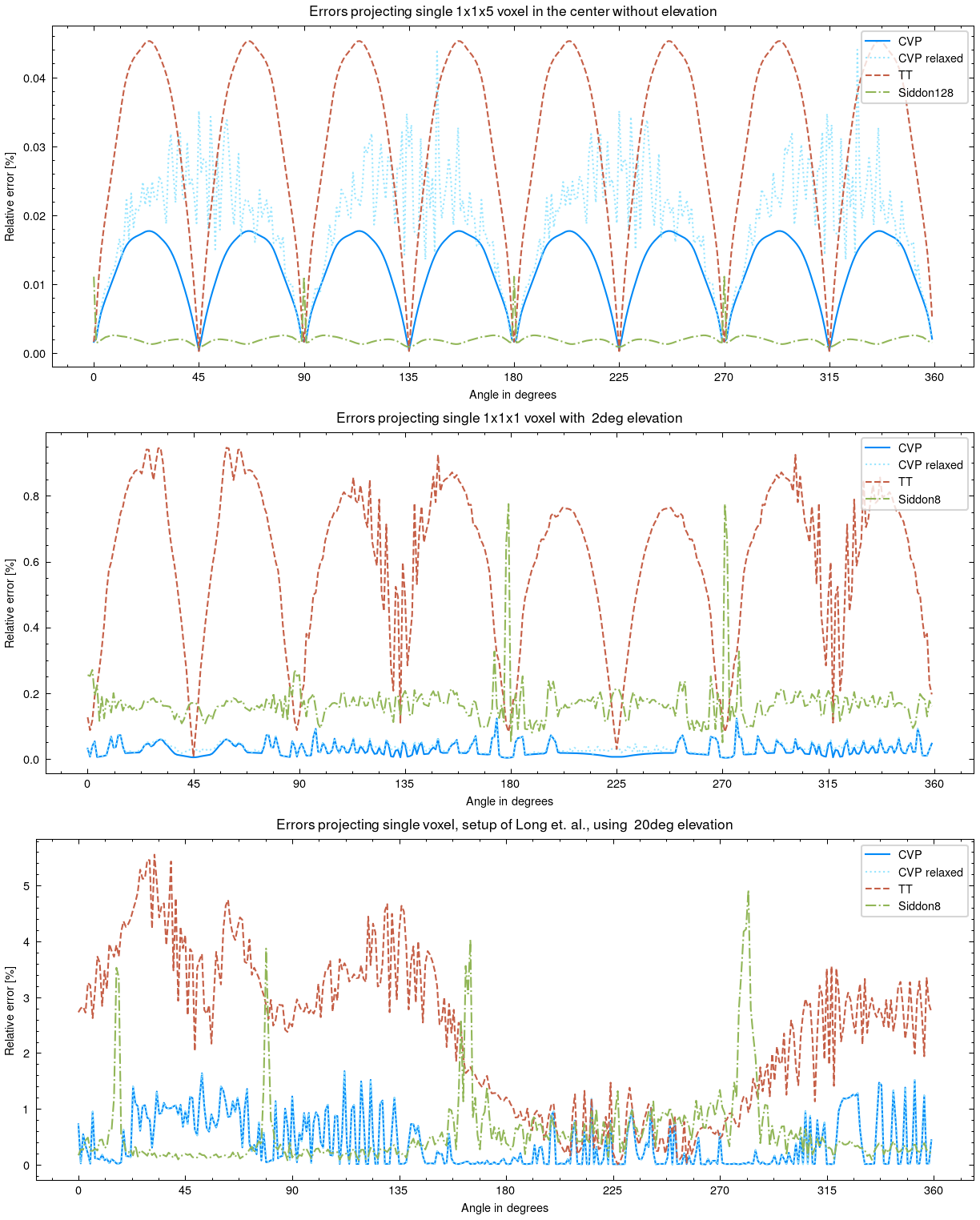
Figure 4: Comparison of projection errors of different projectors at different settings. In the top image, the voxel is placed in the center of rotation is studied. In the middle image, the voxel is outside rotation center shifted so that the elevation and cone beam angles are around $2\text{\,}\mathrm{\SIUnitSymbolDegree}$. The bottom image shows a setup with a voxel projected with a large cone beam angles and elevations.

IV-C Transparency and reproducibility of the results

We believe in the concept of open science. Therefore, not only the software developed by the first author is published under an open source license, we are also publishing all the procedures, scripts, input data and log files, including implementation details, that were used to produce the graphs and tables in the results section. This way, anyone can reproduce our steps on their hardware and compare the results, or use our logs and scripts to compare the results with the underlying data. The files and protocols are published on the website https://kulvait.github.io/KCT_doc/categories/cvp-paper-2020.html.

This is also important for the users of the software, because in the future we can disclose how the run times of the projectors change with new versions of the software or with new hardware.

V Discussion

V-A Elevation correction

A basic version of the algorithm based on Section III-A has been implemented since 2019. The first author has used it to compute hundreds of reconstruction problems as part of his work on improving algorithms for processing CBCT perfusion data. It has been used, for example, for the contributions [5, 6] and two students have used it when writing their theses. It was always clear that it was a very accurate projector roughly comparable to the TT projector.

When preparing this article, projector profiles were compared based on angle. In the problems with non-zero elevation angle, it was interesting to observe that the blue lines representing this projector in Figure 4 mostly stay relatively low, but for certain views the errors have extremes above the TT projector. A closer study of the projection difference profiles showed that in certain situations errors are visible at the top or bottom edge of the projection of a given voxel. Moreover, if it was the edge projecting to the top, there was always insufficient extinction on the topmost, more distant, pixel and almost the same value was overexposed one pixel below. An even closer look yielded the observation that this situation occurs when the upper projection of the center of mass of the slice of the cut through the $x_{1}x_{2}$ plane is almost at the pixel boundary in $\chi_{2}$ direction.

This led to the idea of extending the projected line given by the centre of mass and the $x_{3}$ limits in the plane of the incoming rays by one dimension. So instead of line segments, we will now project rectangles corresponding to given voxels with bases parallel to the bases of these voxels. If the center of mass is projected at the pixel boundary in the direction of $\chi_{2}$, then we project the part of the rectangle above the ray to this center of mass onto the distant top pixel instead of the pixel below it. Of course, we still need to calculate at what distances from the boundary to make the correction and how large, and this increases the computational complexity to some extent. But since this increase is not large especially for the relaxed version of the projector, and since the run times of our projector are much smaller than known implementations of the less accurate TT projector, see Table I and Table II, we decided to present here only the version with elevation correction.

The length of the third dimension is not computed exactly in the current implementation, but using an estimate to speed up the computation, we also assume that the distance from the center of gravity is the same in both directions. Perhaps an accurate calculation would smooth out the remaining extremes of the blue lines in the figure 4. Allowing unequal distances from the centre of gravity would also mean allowing corrections within the projections onto the inner pixels.

This will be the subject of further study, but even without further improvements, the current version of the elevation correction allows us to say that we present the most accurate published projector known, with the exception of ray tracing projectors with extremely large numbers of rays thrown to individual voxels. After all, a projector of comparable accuracy, Siddon8, already uses 64 rays per pixel. To keep error under the projection errors of TT and CVP in the situation with no elevation, see figure 4 top, we need even Siddon128 and Siddon32 is worse from all view angles than unrelaxed CVP.

V-B Speed of the projector

The times of the CVP projector and its relaxed version are listed in tables I and II. We have achieved much better run times than those usually reported for the TT projector with even higher accuracy. To achieve these times, many optimizations were implemented specifically for the GPU hardware as we describe in more detail in the III-C section. The key optimization, is that we compute the cuts through the $x_{1}x_{2}$ planes for each voxel separately. This allows us to run one thread for each voxel and to better partition the problem with respect to the GPU architecture.

V-C Speeding up footprint projectors

One important implication of our work is that similar techniques can speed up the implementation of footprint projectors. The implementation of Long et.al. [11] from 2010 is optimized for CPUs. The algorithm starts with two loops for each row and for each column utilizing the (36). This implementation is being replicated for GPU architectures as well with belief it is optimal, see [15]. Our current TT implementation was designed as a reference and therefore uses double precision. However, it uses the outlined implementation where the main calculation is performed for each voxel separately. The results on the AMD GPU platform, which computes faster in double precision, clearly show the potential of this speedup. We will work on this immediately after this publication.

V-D Non-circular trajectories

One way to consider non-circular trajectories is to take directly the relation (35) and think how to calculate the volumes $|V^{(i,j,k)}_{(m,n)}|$ for a given trajectory. We are not aware of any algorithm that computes cuts for a general orientation of voxels, but this does not mean that there is not one, and for some trajectories it would probably be possible to compute these volumes ad-hoc. As can be seen from the elevation correction example, the more accurate the volume calculation, the more accurate the projector.

V-E Reconstruction

Due to lack of space and time, we do not publish any reconstructions here. The version without elevation correction provides reconstructions mostly indistinguishable from the TT projector. In future work, we will investigate whether the increased accuracy of the algorithm with elevation correction will yield a measurable increase in quality for CT reconstructions.

V-F Software

The software in which these projectors are implemented is not just about them. It is a set of programs for algebraic reconstruction. Originally, the focus was on CT reconstruction using Krylov LSQR and CGLS methods. Gradually other methods were added, most recently a variant of SIRT algorithm accelerated by ordered subsets, see [16, 17]. For example, reconstruction using a relaxed version of CVP with 10 subsets can be run with the following command:

kct-krylov --cvp --barrier --relaxed --elevation-correction --os-sart --os-subset-count 10 input_projections input_projection_matrices output_volume

We are working on regularization of the CT operator, preconditioning of Krylov methods and of course on improvements of the introduced projectors. The first author intends to continue to actively develop the software and present the results in a separate contributions.

V-G Conclusion

This work is part of a four-year postdoctoral research by V. Kulvait under the supervision of G. Rose. The idea of projections of voxel cuts seemed at first to be just an interesting mathematical pun. We nevertheless proceeded to a broader study of the properties of such a projector, including the possibilities of its fast GPU implementation. Many questions remain open, yet we present probably the fastest and most accurate implementation of a CBCT projector in the last decade. And based on the reported projector speeds, which have met with recent improvements in GPU computing, we hope that this work will enable wider deployment of algebraic reconstruction methods in practice.

References

- [1] L. A. Feldkamp, L. C. Davis, and J. W. Kress, “Practical cone-beam algorithm,” Journal of the Optical Society of America A, vol. 1, no. 6, p. 612, 1984.
- [2] H. K. Tuy, “An inversion formula for cone-beam reconstruction,” SIAM Journal on Applied Mathematics, vol. 43, no. 3, pp. 546–552, 1983.
- [3] A. Katsevich, “An improved exact filtered backprojection algorithm for spiral computed tomography,” Advances in Applied Mathematics, vol. 32, no. 4, pp. 681–697, 2004.
- [4] S. Rit, M. V. Oliva, S. Brousmiche, R. Labarbe, D. Sarrut, and G. C. Sharp, “The reconstruction toolkit (RTK), an open-source cone-beam CT reconstruction toolkit based on the insight toolkit (ITK),” Journal of Physics: Conference Series, vol. 489, p. 012079, mar 2014.
- [5] V. Kulvait and G. Rose, “Software Implementation of the Krylov Methods Based Reconstruction for the 3D Cone Beam CT Operator,” in 16th International Meeting on Fully Three-Dimensional Image Reconstruction in Radiology and Nuclear Medicine, 2021.
- [6] H. Haseljić, V. Kulvait, R. Frysch, B. Hensen, F. Wacker, G. Rose, and T. Werncke, “The Application of Time Separation Technique to Enhance C-arm CT Dynamic Liver Perfusion Imaging,” in 16th International Meeting on Fully Three-Dimensional Image Reconstruction in Radiology and Nuclear Medicine, 2021.
- [7] R. L. Siddon, “Fast calculation of the exact radiological path for a three-dimensional CT array,” Medical Physics, vol. 12, no. 2, pp. 252–255, 1985.
- [8] M. Sramek and A. Kaufman, “Fast ray-tracing of rectilinear volume data using distance transforms,” IEEE Transactions on Visualization and Computer Graphics, vol. 6, no. 3, pp. 236–252, 2000.
- [9] H. Zhao and A. Reader, “Fast ray-tracing technique to calculate line integral paths in voxel arrays,” in 2003 IEEE Nuclear Science Symposium. Conference Record (IEEE Cat. No.03CH37515). IEEE, 2003, pp. 2808–2812.
- [10] B. D. Man and S. Basu, “Distance-driven projection and backprojection in three dimensions,” Physics in Medicine and Biology, vol. 49, no. 11, pp. 2463–2475, 2004.
- [11] Y. Long, J. A. Fessler, and J. M. Balter, “3d forward and back-projection for x-ray CT using separable footprints,” IEEE Transactions on Medical Imaging, vol. 29, no. 11, pp. 1839–1850, 2010.
- [12] V. Prasolov and V. Tikhomirov, Geometry, ser. Translations of Mathematical Monographs. American Mathematical Society, 2001.
- [13] joriki (https://math.stackexchange.com/users/6622/joriki), “Area of the sphere that gets projected to rectangle,” Mathematics Stack Exchange, uRL:https://math.stackexchange.com/q/3540309 (version: 2020-02-09). [Online]. Available: https://math.stackexchange.com/q/3540309
- [14] I. Todhunter, Spherical trigonometry, J. G. Leathem, Ed. Macmillan and Company, 1914.
- [15] T. Pfeiffer, R. Frysch, and G. Rose, “Two extensions of the separable footprint forward projector,” in 16th International Meeting on Fully Three-Dimensional Image Reconstruction in Radiology and Nuclear Medicine, 2021.
- [16] H. Hudson and R. Larkin, “Accelerated image reconstruction using ordered subsets of projection data,” IEEE Transactions on Medical Imaging, vol. 13, no. 4, pp. 601–609, 1994.
- [17] J. Gregor and T. Benson, “Computational analysis and improvement of SIRT,” IEEE Transactions on Medical Imaging, vol. 27, no. 7, pp. 918–924, jul 2008.