Pre and Post Counting for Scalable Statistical-Relational Model Discovery

Abstract

Statistical-Relational Model Discovery aims to find statistically relevant patterns in relational data. For example, a relational dependency pattern may stipulate that a user’s gender is associated with the gender of their friends. As with propositional (non-relational) graphical models, the major scalability bottleneck for model discovery is computing instantiation counts: the number of times a relational pattern is instantiated in a database. Previous work on propositional learning utilized pre-counting or post-counting to solve this task. This paper takes a detailed look at the memory and speed trade-offs between pre-counting and post-counting strategies for relational learning. A pre-counting approach computes and caches instantiation counts for a large set of relational patterns before model search. A post-counting approach computes an instantiation count dynamically on-demand for each candidate pattern generated during the model search. We describe a novel hybrid approach, tailored to relational data, that achieves a sweet spot with pre-counting for patterns involving positive relationships (e.g. pairs of users who are friends) and post-counting for patterns involving negative relationships (e.g. pairs of users who are not friends). Our hybrid approach scales model discovery to millions of data facts.

Introduction

Statistical-Relational Learning (SRL) aims to construct statistical models that extract knowledge from complex relational and network data. SRL model construction searches through a space of possible models, scoring different candidate models to find a (local) statistical score optimum. SRL models are typically composed of local dependency patterns, represented with edges in a model graph or clauses in logical syntax. The main computational burden in model scoring is instance counting, determining the number of times that a local pattern defined by the model occurs in the dataset. A key technique to scale counting for large and complex datasets is caching local instance counts and statistical scores. Caching trades memory for model search time and is standard in graphical model search for propositional (i.i.d.) data (e.g.  (The Tetrad Group 2008)). There are two basic approaches to counts caching (Lv, Xia, and Qian 2012): Pre-counting builds up a large cache of local pattern counts before the model search phase. Post-counting computes local instance counts only for patterns generated during model search and then adds them (or the resulting scores) to a cache in case the pattern is revisited later during model search. This paper compares pre and post counting for relational model search.

Why Relational Counting Is Hard.

To understand the pros and cons of different count caching strategies, we briefly review why relational counting problems are fundamentally different from, and harder than, counting in propositional data. For propositional data, a conjunctive pattern specifies a set of attribute values for singletons of entities; for example, the set of female users over 40. Counting then requires only filtering, finding the subset of existing entities matching the pattern. Relational data specify linked pairs of entities, like users who are friends (assuming binary relationships), where two new counting problems arise:

1. Relational patterns may involve $k$-tuples of entities/nodes. For example, a triangle involves 3 nodes. A naive approach to counting would require enumerating $n^{k}$ $k$-tuples of entities. In an SQL table representation of relational data, counting for $k$-tuples of entities involves table JOINs; we therefore term it the JOIN problem. The JOIN problem has been extensively studied in the database community as part of SQL query evaluation (COUNT(*) queries).

2. Relational patterns may involve negative relationships, pairs of entities not listed in the data. For example, we may wish to find the number of women users who have not rated a horror movie. We term this the negation problem. The JOIN and negation problems both involve pattern instances that are not subsets of the given data tuples.

Pre vs. Post Counting: Advantages and Disadvantages.

The main advantage of pre-counting is that the data is scanned only once to build up a cache. In particular, the number of table JOINs is minimized, as our experiments show. Also, the cache can be built incrementally using dynamic programming by computing counts for longer patterns from shorter ones. For example, in relational data, counts with a relationship chain length of l can be built up from relationship chains of length 1, 2, …, l - 1 (Yin et al. 2004; Schulte and Qian 2019). The main disadvantage of pre-counting is building a large cache of counts for complex patterns, with only a fraction likely to be required for model selection. For example, pre-counted dependency patterns may involve 20 predicates, whereas model search rarely considers clauses with more than 5.

The main advantage of post-counting is that instances are counted only for patterns generated by the model search. The disadvantage is that each pattern evaluation requires a new data access with potentially expensive table JOINs.

A high-level summary of our empirical findings is that because of the JOIN problem, pure post-counting scales substantially worse than pure pre-counting. At the same time, the negation problem is challenging for the large patterns built up in pre-counting. Therefore, we introduce a hybrid method that uses pre-counting for the JOIN problem and post-counting for the negation problem. The hybrid method leverages the Möbius Join algorithm which computes instance counts for relational patterns that may involve positive and negative relationships (Qian, Schulte, and Sun 2014). The Möbius Join is an inclusion-exclusion technique that requires no further data accesses to the original data, and hence no further table JOINs.

Our contributions may be summarized as follows:

• Investigating the strengths and weaknesses of pre/post count counting strategies for different relational dataset properties.

• Describing a new hybrid count caching method, tailored towards relational data, that for many datasets combines the strengths of both pre and post counting. Hybrid counting scales to millions of data facts (database rows).

Related Work

We selectively discuss the most relevant topics from previous SRL work.

Language Bias. We consider first-order relational patterns that only involve types of individuals, not specific individuals (e.g. $\mathit{Friend(X,Y)}$ not $\mathit{Friend(joe,Y)}$). While this is a common restriction in SRL (Ravkic, Ramon, and Davis 2015; Schulte et al. 2016; Kimmig, Mihalkova, and Getoor 2014), it limits the applicability of our results to methods that search for clauses involving individuals, such as Boostr (Natarajan et al. 2012). Our experiments investigate learning directed models (first-order Bayesian networks), but our observations about the fundamental JOIN and negation problems apply to other SRL models as well.

Search Space: Predicates vs. Clauses. Inspired by graphical models, a tradition in SRL is to search for dependencies between predicates, typically represented by links in a model graph. For example, an edge $\mathit{intelligence(S)}\leftarrow\mathit{grade(S,C)}$ may represent that the grades of a student predicts their intelligence. Another tradition, inspired by inductive logic programming, searches for dependencies among predicate values, typically represented by clauses (e.g. $\mathit{intelligence(S)=high}$ :- $\mathit{grade(S,C)=A}$). Since the predicate space is smaller than that of predicate values, it supports a more efficient model search (Kersting and De Raedt 2007; Friedman et al. 1999; Khosravi et al. 2010) at the expense of expressive power (Khosravi et al. 2012). With regard to instance counting, a predicate dependency groups together a set of clauses (one for each combination of parent-child values). Model evaluation requires instance counting for the entire clause set, which is often more efficient than separate counting, if the data for the same predicates is stored together. For example if in an SQL table, grades are stored in the same table column, then counting instances for different grades requires only a single table JOIN. While our experiments evaluate only predicate-level search, we expect that the general trends apply also to clause-level search.

Approximate vs. Exact Counting. Several SRL approaches have increased scalability by aiming for approximate counting, which is often sufficient for model evaluation (e.g. (Das et al. 2019)). In this paper we use only exact counts, obtained by SQL queries. Other SRL work has also shown the usefulness of SQL optimization for obtaining instance counts (e.g. (Niu et al. 2011)). Approximate counting speeds up the instance for a single pattern, which is orthogonal to our topic of counts caching; caches can be used for both approximate and exact counts. We discuss approximate counting further in the future work section. Another type of approximation is negative sampling of unlinked node pairs, which adds extra node pairs to the data (Nickel et al. 2016). Computationally, negative sampling solves the negation problems but increases the JOIN problem. Caching counts for negative sampling is an interesting direction for future work.

Graphical Model Background

We choose the FactorBase system (Schulte and Qian 2019) for experimentation and to illustrate computational counting challenges. FactorBase learns a first-order Bayesian network (BN) (Poole 2003; Wang et al. 2008) for a relational dataset. An example of a first-order Bayesian network can be found in Figure 1.

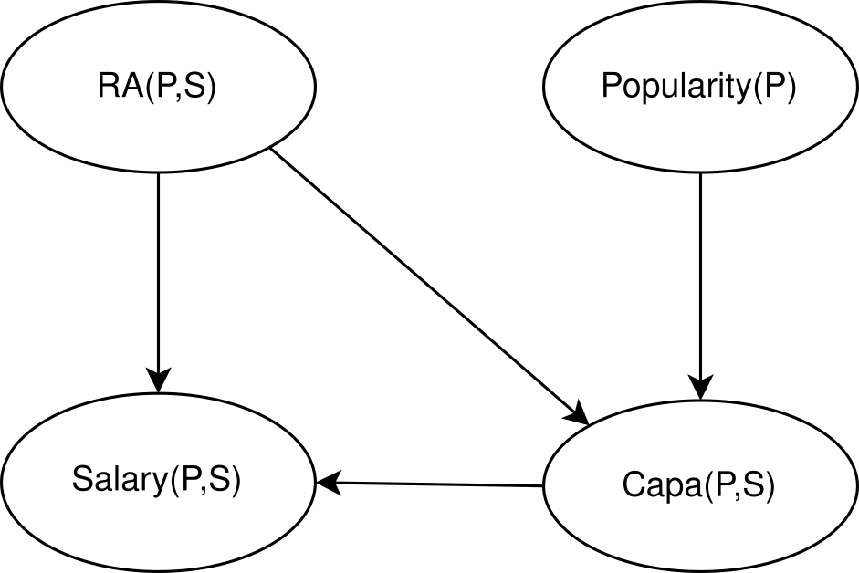
Figure 1: An example of a first-order Bayesian network.

FactorBase is an appropriate benchmark as it achieves SOTA scalability (Schulte et al. 2016). We focus on our description on fundamental issues associated with relational counting that we expect to generalize to other systems. In the Limitations section, we discuss design options not explored in our experiments.

As an example model score, the BDeu score for a given BN $B$ and dataset $D$ is defined in Equation 1.

$$BDeu(B,D)=\log{\left(P(B)\right)}+\sum_{i=1}^{n}\sum_{j=1}^{q_{i}}\left(\log{\left(\frac{\Gamma\left(\frac{N^{\prime}}{q_{i}}\right)}{\Gamma\left(N_{ij}+\frac{N^{\prime}}{q_{i}}\right)}\right)}+\sum_{k=1}^{r_{i}}\log{\left(\frac{N_{ijk}+\frac{N^{\prime}}{r_{i}q_{i}}}{\Gamma\left(\frac{N^{\prime}}{r_{i}q_{i}}\right)}\right)}\right)$$ (1)

A description of the terms can be found in Table 1. A parent configuration for node $i$ is a tuple of values, one for each parent.

Example.

Let node $i$ be $\mathit{Salary(P,S)}$ with 4 possible values $r_{i}$ (LOW, MED, HIGH, N/A). Together with its parents, node $i$ forms the model family, which expresses a relational dependency pattern $\mathit{RA(P,S),Capa(P,S)}\rightarrow$
$\mathit{Salary(P,S)}$. Suppose we assign index $j$ to the parent configuration $\mathit{RA(P,S)=T,Capa(P,S)=4}$. Then $N_{ij}$ counts how often this configuration occurs in the dataset $D$: the number of professor-student pairs such that the student is an RA for the professor with a high capability of 4. Suppose we assign index $k$ to the salary value HIGH. Then $N_{ijk}$ counts how often the parents are in configuration $j$ and the child node takes on value $k$: the number of professor-student pairs such that the student is an RA for the professor with a high capability of 4 and receives a HIGH salary. In Table 3, this count equals 5. In terms of clauses, $N_{ijk}$ represents the instantiation count of the clause $\mathit{RA(P,S)=T},\mathit{Capa(P,S)=4\rightarrow Salary(P,S)=HI}$-$\mathit{GH}$.

Variable	Description
$n$	Number of nodes in the model graph
$r_{i}$	Number of possible values for node $i$
$q_{i}$	Number of parent configurations for node $i$
$N^{\prime}$	Equivalent sample size.
$N_{ij}$	Number of occurrences where node $i$ has its parents in the $j^{th}$ configuration.
$N_{ijk}$	Number of occurrences where node $i$ is assigned its $k^{th}$ value and its parents are assigned the $j^{th}$ configuration.

Table 1: Terms in the BDeu scoring metric, which is used to score BNs such as the one found in Figure 1.

Schulte and Gholami showed how the BDeu score can be adapted for multi-relational data (2017). The count operations required are essentially the same between the relational BDeu score and the propositional score shown, and similar for other BN scores. The most computationally expensive part of BDeu, and many other scoring metrics, is generating instantiation or frequency counts to obtain the $N_{ij}$ and $N_{ijk}$ values. Instance counts can be represented in a contingency table (ct-table): for a list of variables $V_{1},\ldots,V_{m}$, the table contains a row for each value tuple $v_{1},\ldots,v_{m}$, and records how many times this value combination occurs in the data set (Lv, Xia, and Qian 2012; Qian, Schulte, and Sun 2014). Following (Lv, Xia, and Qian 2012), we use ct-tables as caches for instance counts.

Figure 2: A relationship lattice for two relationships (students register in courses and work as RAs for professors) where each node in the graph is a lattice point.

Positive ct-table	Negative ct-table	Learning Method
Lattice Point	Lattice Point	PRECOUNT
Family	Family	ONDEMAND
Lattice Point	Family	HYBRID
Family	Lattice Point	IMPOSSIBLE

Table 2: Summary of possible methods to consider for computing ct-tables from a relational database based on the inputs for creating the positive and negative ct-tables.

Computing Relational Contingency Tables

We use the method of (Qian, Schulte, and Sun 2014), as implemented in FactorBase. As discussed under Related Work, other methods may be employed as well, such as approximate counting. In a relational ct-table, a key role is played by relationship indicator variables that indicate whether a relationship holds (e.g. $\mathit{Registered(S,C)}=T$ or $\mathit{Registered(S,C)}$) or not (e.g. $\mathit{Registered(S,C)}=F$ or $\neg\mathit{Registered(S,C)}$). In a positive ct-table, all relationship indicator variables are set to $T$ (true). A complete ct-table contains values for both true and false relationships; see Table 3 for illustration. The last 9 rows form the positive ct-table. The predicate RA(P,S) represents that a student is an RA for a professor, and the attributes Capa(P,S) and Salary(P,S) represent a student’s salary and capability when they are the RA for a given professor.

Count	Capa(P,S)	RA(P,S)	Salary(P,S)
203	N/A	F	N/A
5	4	T	HIGH
4	5	T	HIGH
2	3	T	HIGH
1	3	T	LOW
2	2	T	LOW
2	1	T	LOW
2	2	T	MED
4	3	T	MED
3	1	T	MED

Table 3: A contingency table represents instantiation counts of a conjunctive condition in a database. For example, the last row shows that the number of instances (groundings) is 3 for the assignment Capa(P,S) = 1, RA(P,S) = T, Salary(P,S) = MED. Numbers are chosen for illustration.

FactorBase uses a 2-stage approach to compute a relational ct-table, which is described as follows:

1. Input: A list of variables $V_{1},\ldots,V_{m}$ and a relational dataset $D$.

2. Generate a positive ct-table $\mathit{ct}_{+}(\mathbf{R})$ for each relationship lattice point $\mathbf{R}$. FactorBase uses SQL INNER JOINs to compute a ct-table for existing relationships (a COUNT(*) query with a GROUP BY clause).

3. Extend $\mathit{ct}_{+}(\mathbf{R})$ to a complete ct-table $\mathit{ct}(\mathbf{R})$. FactorBase uses the Möbius Join for this step.

The Möbius Join is an inclusion-exclusion technique whose details are somewhat complex and not necessary for this work. The main points of importance for this research are as follows:

1. Given a positive ct-table, where all relationships are true, the Möbius Join returns a ct-table for both existing and non-existing relationships without further access of the original data.

2. The runtime cost of the Möbius Join as shown by (Qian, Schulte, and Sun 2014) is the following:

   $$O\left(r\log{\left(r\right)}\right)$$ (2)

   where $r$ is the number of rows in the output ct-table.

Next we consider approaches for computing relational ct-tables. The basic choices are to compute a global ct-table for all variables. Or a smaller ct-table for those associated with a family (local pattern). Table 2 lays out the options, which we discuss in the next sections.

PRECOUNT Counts Caching Method

Chains of relationships form a lattice that can be used to structure relational model search (Schulte and Khosravi 2012; Yin et al. 2004; Friedman et al. 1999); see  Figure 2. For instance, the learn-and-join model search (Schulte and Khosravi 2012) builds up BNs for each lattice point in a bottom-up fashion. The pre-count method computes a ct-table for each relationship chain, for all variables associated with the chain. For example, for the lattice point $\mathit{Registered(S,C)}$, the variables include all attributes of students, courses, and the registration link (e.g. $\mathit{grade})$. The high-level structure of pre-count caching is illustrated in Algorithm 1. Given a large ct-table, we can compute a smaller ct-table for a subset of columns by summing out the unwanted columns; this operation is called projection (Lv, Xia, and Qian 2012). For example, given a ct-table for the lattice point $\mathit{Registered(S,C)}$ with columns for all attributes of students, projection can be used to obtain a ct-table for just one student attribute. During structure search, pre-count computes ct-tables for local families from the applicable lattice point ct-table using projection.

PRECOUNT will generate ct-tables for each relationship chain that grow in size as we increase the chain length, which is a key factor for its computational performance.

1:for each $\mathit{latticePoint}\;LP\in\mathit{relationshipLattice}$ do

2:     $\mathit{ct}_{+}(LP)\leftarrow\textsc{InnerJoin}(\textsc{Tables}(LP))$

3:     $\mathit{ct}(LP)\leftarrow\textsc{M\"{o}biusJoin}(\mathit{ct}_{+}(LP))$

4:end for

5:for each $\mathit{family}\in\mathit{structureLearning}$ do

6:     $\mathit{ct}(\mathit{family})\leftarrow\textsc{Project}(\mathit{ct}(LP),\mathit{family})$

7:     $\mathit{score}\leftarrow\textsc{BDeu}(\mathit{ct}(\mathit{family}))$

8:end for

Algorithm 1 The PRECOUNT method: pre-compute ct-tables for each lattice point.

Contingency Table Growth Rate for PRECOUNT

Given a database table $\mathit{T}$ with $\mathit{C}$ columns where each column contains $\leq\mathit{V}$ values each, the size (number of rows) of $\mathit{T}$ can be upper bound using the following expression:

$$\textsc{Size}(T)=O\left(V^{C}\right)$$ (3)

From Equation 3 we see that ct-tables grow exponentially with respect to the number of columns when using PRECOUNT. The alternative is to generate many small tables that are equivalent to the single large one, but grow in size at a slower rate. This is the approach used by ONDEMAND.

ONDEMAND Counts Caching Method

This is a relational adaptation of the single-table post-counting concept from (Lv, Xia, and Qian 2012). ONDEMAND computes ct-tables for families not relationship chains as PRECOUNT does. Family ct-tables are much smaller than relationship chain ct-tables, roughly constant-size in practice. ONDEMAND generates a ct-table for each family of nodes that is scored.

1:for each $\mathit{family}\in\mathit{structureLearning}$ do

2:     $\mathit{ct}_{+}(\mathit{family})\leftarrow\textsc{InnerJoin}(\textsc{Tables}(\mathit{family}))$

3:     $\mathit{ct}(\mathit{family})\leftarrow\textsc{M\"{o}biusJoin}(\mathit{ct}_{+}(\mathit{family}))$

4:     $\mathit{score}\leftarrow\textsc{BDeu}(\mathit{ct}(\mathit{family}))$

5:end for

Algorithm 2 The ONDEMAND method: compute ct-tables for each family during structure search.

Contingency Table Growth Rate for ONDEMAND

Given a table $\mathit{T}$ with $\mathit{C}$ columns, with each column containing $\leq\mathit{V}$ values each and $\mathit{k}$ parents to choose from, the total size of the equivalent multi-table version of the single large one can be upper bound using the following expression:

$$\textsc{Size}(T)=O\left(\mathit{C}\binom{\mathit{C}-1}{k}V^{k+1}\right)$$ (4)

From Equation 4 we see that ct-tables grow exponentially with respect to the size of the family of nodes being scored when using ONDEMAND. Therefore, ONDEMAND is advantageous only if the family sizes generated during search are small. Several facts support that the family sizes generated will be small. The BDeu equation (Equation 1) shows that large families incur an exponential penalty in the model score; the same holds for other standard scores. The literature on BN learning states that empirically, the maximum number of parents is typically 4 (Lv, Xia, and Qian 2012; Tsamardinos, Brown, and Aliferis 2006). For the datasets in our study, we also observe that the BN nodes have small indegrees. Table 4 shows the mean number of parents per node in the BN learned for the various databases used in the experiments. While the size of each ct-table generated by ONDEMAND is small, the method generates many positive ct-tables and as a result executes many expensive table JOINs.

HYBRID Counts Caching Method

This is our new alternative method for computing ct-tables from a relational database. The pseudocode for it is found in Algorithm 3. HYBRID combines the strengths from PRECOUNT and ONDEMAND and has the following characteristics:

• Like PRECOUNT, it generates a positive ct-table $\mathit{ct}_{+}(\mathbf{R})$ for each relationship lattice point $\mathbf{R}$.

• Like ONDEMAND, it generates a complete ct-table $\mathit{ct}(\mathbf{F})$ for each family of nodes $\mathbf{F}$ being scored.

1:for each $\mathit{latticePoint}\;LP\in\mathit{relationshipLattice}$ do

2:     $\mathit{ct}_{+}(LP)\leftarrow\textsc{InnerJoin}(\textsc{Tables}(LP))$

3:end for

4:for each $\mathit{family}\in\mathit{structureLearning}$ do

5:     $\mathit{ct}_{+}(\mathit{family})\leftarrow\textsc{Project}(\mathit{ct}_{+}(LP),\mathit{family})$

6:     $\mathit{ct}(family)\leftarrow\textsc{M\"{o}biusJoin}(\mathit{ct}_{+}(\mathit{family}))$

7:     $\mathit{score}\leftarrow\textsc{BDeu}(\mathit{ct}(family))$

8:end for

Algorithm 3 The HYBRID method: pre-compute positive ct-tables for each lattice point and compute ct-tables for each family during structure search.

The HYBRID method uses the large relationship chain ct-table $\mathit{ct}_{+}(\mathbf{R})$ as a cache to replace expensive JOINs with projections (line 5). Assuming that local families are small, extending positive ct-tables to complete ones is relatively fast; see Equation 2. Both HYBRID and PRECOUNT assume that the overall number of columns/relationships in the database is moderate so that computing the positive ct-table $\mathit{ct}_{+}(\mathbf{R})$ using all columns of a given lattice point is feasible. If the overall number of columns/relationships is too large to compute the $\mathit{ct}_{+}(\mathbf{R})$ tables, ONDEMAND must be used instead of PRECOUNT or HYBRID.

Empirical Evaluation

Hardware and Datasets

Jobs were submitted to Compute Canada’s Cedar high performance cluster using Slurm version 20.11.4. Each job requested one 2.10GHz Intel Broadwell processor and enough RAM to process each dataset. Using MariaDB version 10.4 Community Edition, 8 real databases of varying size and complexity were supplied as input to FactorBase for each method in Table 2. Of these 8 databases, 7 are benchmark databases that have been used in previous studies where the scalability of methods for constructing BNs from relational databases was studied (Schulte and Qian 2019). Visual Genome is added to this list of benchmark databases due to the large amount of data and number of relationship tables it possesses compared to the other 7 databases; see Table 4. Visual Genome is the only dataset that required preprocessing where ternary relationships had to be converted into binary relationships using the standard star schema approach (Ullman 1982).

Database	Row Count	# Relationships	MP/N
UW	712	2	1.6
Mondial	870	2	1.3
Hepatitis	12,927	3	1.7
Mutagenesis	14,540	2	1.6
MovieLens	74,402	1	1.4
Financial	225,887	3	1.9
IMDb	1,063,559	3	3.4
Visual Genome	15,833,273	8	0.5

Table 4: Databases used as input to FactorBase with their associated total number of table rows, number of relationship tables they contain, and the mean number of parents per node (MP/N) in the BNs learned when using FactorBase and the BDeu score.

DB	Estimated Total $\mathit{ct}(\mathit{family})$ Row Count	$\mathit{ct}(\mathit{database})$ Total Row Count
MovieLens	816	239
Mutagensis	6075	1631
UW	15318	2828
Visual Genome	2923968	20447
Mondial	55800	1738867
Financial	930468	3013006
Hepatitis	176220	12374892
IMDb	33040	15537457

Table 5: Size of the ct-tables generated for each family scored and the entire database. The $\mathit{ct}(family)$ column is for ONDEMAND and HYBRID while the $\mathit{ct}(database)$ column is for PRECOUNT. Databases are sorted in ascending order based on the size of the ct-table generated for the entire database.

Runtime Metrics Reported

Since the focus of this research is reducing the time it takes to generate ct-tables for large relational databases, we break down ct-table construction time into the following 3 components: (1) Metadata (2) Positive ct-table ($\mathit{ct}_{+}$) (3) Negative ct-table ($\mathit{ct}_{-}$).

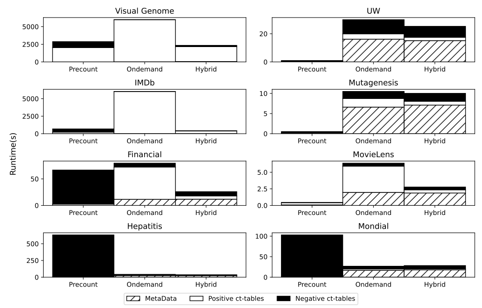
Figure 3: Comparison of the time it takes for ct-tables to be constructed for PRECOUNT, ONDEMAND, and HYBRID. For IMDb and Visual Genome, ONDEMAND failed to complete within the allotted time so only partial results have been included for those datasets in this figure.

MetaData

This component consists of various metadata specifying the relational schema (syntax) that is extracted and generated from the input database. It includes the extraction of the first-order logic information related to the ct-tables being generated, generation of the relationship lattice, and generation of the metaqueries, which are used to construct the dynamic SQL query statements for performing the necessary database queries.

Positive ct-table

This component consists of the $\mathit{ct}_{+}$ counting information, which is made of two types of counting queries. Counts for entity tables are generated with a simple GROUP BY query involving no JOINs. To generate positive ct-tables for relationship chains, we used a GROUP BY SQL query with INNER JOINs.

Negative ct-table

This component consists of the Möbius Join so it is made of the time it takes to generate the counts for all combinations of negative relationships.

Runtime Results

Figure 3 shows the cumulative time it takes to construct all the ct-tables for a given database. The times are broken down into the 3 components of MetaData, Positive ct-table ($\mathit{ct}_{+}$), and Negative ct-table ($\mathit{ct}_{-}$) as described previously. For ONDEMAND, the execution of FactorBase exceeded a runtime limit of 100 minutes on IMDb and Visual Genome. Hence their results are omitted, or are incomplete if included in a figure. As expected, due to the large size of the ct-tables being generated, PRECOUNT requires substantially more time to generate the negative ct-table than the two comparison methods. Overall ONDEMAND performs much worse than PRECOUNT, mostly due to the time it takes to generate the local positive ct-tables, especially for the large databases like IMDb and Visual Genome. HYBRID on the other hand performs better than PRECOUNT on several of the databases. We analyse this improvement in detail next.

Negative ct-tables

The reason for the general speed-up in negative ct-table construction time is that HYBRID generates smaller ct-tables (see Equations 2 and 4).

Some databases are exceptions to this trend (UW, Mutagenesis and MovieLens). Here the local ct-tables are similar in size to the global one, so the number of ct-tables dominates the relative performance (rather than their size). For further evidence of this explanation, Table 5 shows that for the databases where HYBRID does worse than PRECOUNT, the total number of rows for the ct-tables generated when using HYBRID exceeds the number of rows for the global ct-table generated when using PRECOUNT.

Positive ct-tables

The positive ct-tables for each family scored by HYBRID are generated by projecting the information from the full positive ct-tables for the lattice points. Therefore, scoring a family does not require further table JOINs. Although HYBRID performs better than PRECOUNT for most of the databases experimented with, there are a few cases where PRECOUNT does better. This is mainly a result of the MetaData component for HYBRID taking substantially longer due to overhead costs, and also due to the Negative ct-table component.

MetaData

Figure 3 reveals that HYBRID inherited ONDEMAND’s increased overhead to generate the metadata, which is shown to be negligible for PRECOUNT. Although the metadata overhead is a bottleneck only for ONDEMAND and HYBRID, it does not hurt scalability: the Metadata component is prominent for small databases like Mondial and UW, but essentially disappears for large databases like IMDb and Visual Genome.

Memory Profiling

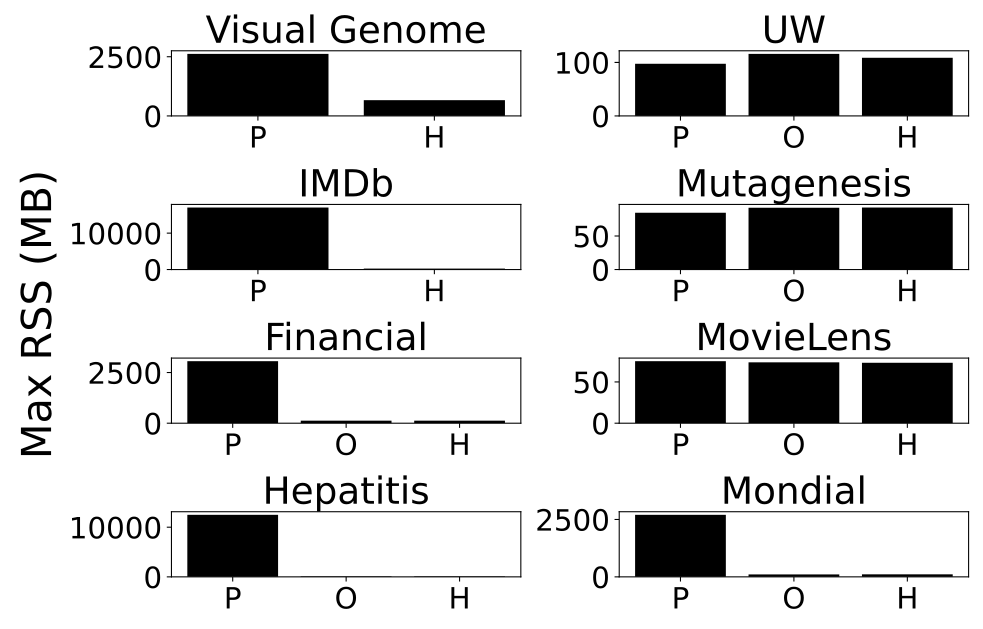
Figure 4: Comparison of the maximum resident set size used by the Java portion of FactorBase when constructing ct-tables for PRECOUNT (P), ONDEMAND (O), and HYBRID (H). Results have been omitted for ONDEMAND in the cases where it failed to complete within the allotted time.

Figure 4 compares the peak memory used when processing the various databases. It shows that PRECOUNT is generally more memory intensive than ONDEMAND and HYBRID. However, there are 3 databases where PRECOUNT uses similar amounts of memory. These 3 databases correspond to the ones in Figure 3 where PRECOUNT performs the best for the Negative ct-table component. In addition, Table 5 shows in these 3 databases the total size of the ct-tables generated using ONDEMAND and HYBRID exceeded the size of the global ct-table generated by PRECOUNT for the entire database. This observation suggests that the reason why PRECOUNT does better on these databases is that they are all generating negative ct-tables similar in size. Recall by Equation 2 the time to generate ct-tables depends on the size of the tables being generated. Also recall that ONDEMAND and HYBRID generate more ct-tables than PRECOUNT, which explains their greater runtime for generating the negative ct-tables.

Limitations and Future Work

We discuss parts of the count-cache design space that we have not covered in our experiments.

Pre-Count Variants. Instead of storing instance counts for complete patterns, an intermediate approach is to store additional local information before model search that facilitates post-counting. An example is tuple ID propagation (Yin et al. 2004). The general idea of tuple ID propagation is that instead of performing an expensive JOIN operation, for each node and relationship type, we store the set of linked node IDs. A table JOIN is then replaced by ID propagation. Compared to the lattice pre-count approach, tuple ID propagation scales well in the number of data columns (predicates) but less well in the number of nodes (rows). Tuple ID propagation may be suitable for expanding the search space to include clauses with individuals since it expands the data with individual information.

Approximate Counting may make a purely post-counting method feasible even for large datasets. Our experiments suggest that it would have to be orders of magnitude more efficient than SQL JOINs to make ONDEMAND competitive with PRECOUNT.

Conclusion

The key computational burden in learning SRL models from multi-relational data is obtaining the pattern instantiation counts that summarize the sufficient statistics (frequencies of conjunctions of relevant predicate values). Our research has investigated two approaches to caching relational counts, before and during SRL model search. Each approach has different implications for two counting challenges fundamental to relational learning: the JOIN problem (counting for chains of existing relationships) and the negation problem (counting for non-existing relationships). We find that for many databases, the most scalable solution is a hybrid approach, which uses pre-counting before model search for the JOIN problem, and post-counting for the negation problem.

References

- Das et al. (2019) Das, M.; Dhami, D. S.; Kunapuli, G.; Kersting, K.; and Natarajan, S. 2019. Fast relational probabilistic inference and learning: Approximate counting via hypergraphs. In Proceedings of the AAAI Conference on Artificial Intelligence, volume 33, 7816–7824.
- Friedman et al. (1999) Friedman, N.; Getoor, L.; Koller, D.; and Pfeffer, A. 1999. Learning probabilistic relational models. In IJCAI, 1300–1309. Springer-Verlag.
- Kersting and De Raedt (2007) Kersting, K.; and De Raedt, L. 2007. Bayesian Logic Programming: Theory and Tool. In Introduction to Statistical Relational Learning, chapter 10, 291–318. MIT Press.
- Khosravi et al. (2012) Khosravi, H.; Schulte, O.; Hu, J.; and Gao, T. 2012. Learning Compact Markov Logic Networks With Decision Trees. Machine Learning 89(3): 257–277.
- Khosravi et al. (2010) Khosravi, H.; Schulte, O.; Man, T.; Xu, X.; and Bina, B. 2010. Structure Learning for Markov Logic Networks with Many Descriptive Attributes. In AAAI, 487–493.
- Kimmig, Mihalkova, and Getoor (2014) Kimmig, A.; Mihalkova, L.; and Getoor, L. 2014. Lifted graphical models: a survey. Machine Learning 1–45.
- Lv, Xia, and Qian (2012) Lv, Q.; Xia, X.; and Qian, P. 2012. A fast calculation of metric scores for learning Bayesian network. International Journal of Automation and Computing 9: 37–44. URL http://dx.doi.org/10.1007/s11633-012-0614-8.
- Natarajan et al. (2012) Natarajan, S.; Khot, T.; Kersting, K.; Gutmann, B.; and Shavlik, J. W. 2012. Gradient-based boosting for statistical relational learning: The relational dependency network case. Machine Learning 86(1): 25–56.
- Nickel et al. (2016) Nickel, M.; Murphy, K.; Tresp, V.; and Gabrilovich, E. 2016. A review of relational machine learning for knowledge graphs. Proceedings of the IEEE 104(1): 11–33.
- Niu et al. (2011) Niu, F.; Ré, C.; Doan, A.; and Shavlik, J. W. 2011. Tuffy: Scaling up Statistical Inference in Markov Logic Networks using an RDBMS. PVLDB 4(6): 373–384.
- Poole (2003) Poole, D. 2003. First-order probabilistic inference. In IJCAI.
- Qian, Schulte, and Sun (2014) Qian, Z.; Schulte, O.; and Sun, Y. 2014. Computing Multi-Relational Sufficient Statistics for Large Databases. In Li, J.; Wang, X. S.; Garofalakis, M. N.; Soboroff, I.; Suel, T.; and Wang, M., eds., Proceedings of the 23rd ACM International Conference on Conference on Information and Knowledge Management, CIKM 2014, Shanghai, China, November 3-7, 2014, 1249–1258. ACM. doi:10.1145/2661829.2662010. URL https://doi.org/10.1145/2661829.2662010.
- Ravkic, Ramon, and Davis (2015) Ravkic, I.; Ramon, J.; and Davis, J. 2015. Learning relational dependency networks in hybrid domains. Machine Learning 100(2): 217–254.
- Schulte and Gholami (2017) Schulte, O.; and Gholami, S. 2017. Locally Consistent Bayesian Network Scores for Multi-Relational Data. In Proceedings of the International Joint Conference on Artificial Intelligence (IJCAI), 2693–2700. URL “url–https://www.ijcai.org/proceedings/2017/0375.pdf˝.
- Schulte and Khosravi (2012) Schulte, O.; and Khosravi, H. 2012. Learning graphical models for relational data via lattice search. Mach. Learn. 88(3): 331–368. doi:10.1007/s10994-012-5289-4. URL https://doi.org/10.1007/s10994-012-5289-4.
- Schulte and Qian (2019) Schulte, O.; and Qian, Z. 2019. FACTORBASE: multi-relational structure learning with SQL all the way. Int. J. Data Sci. Anal. 7(4): 289–309. doi:10.1007/s41060-018-0130-1. URL https://doi.org/10.1007/s41060-018-0130-1.
- Schulte et al. (2016) Schulte, O.; Qian, Z.; Kirkpatrick, A. E.; Yin, X.; and Sun, Y. 2016. Fast learning of relational dependency networks. Machine Learning 1–30. ISSN 1573-0565. doi:10.1007/s10994-016-5557-9. URL http://dx.doi.org/10.1007/s10994-016-5557-9.
- The Tetrad Group (2008) The Tetrad Group. 2008. The Tetrad Project. Http://www.phil.cmu.edu/projects/tetrad/.
- Tsamardinos, Brown, and Aliferis (2006) Tsamardinos, I.; Brown, L. E.; and Aliferis, C. F. 2006. The Max-Min Hill-Climbing Bayesian Network Structure Learning Algorithm. Machine Learning 65(1): 31–78.
- Ullman (1982) Ullman, J. D. 1982. Principles of Database S¡ystems. W. H. Freeman & Co., 2 edition.
- Wang et al. (2008) Wang, D. Z.; Michelakis, E.; Garofalakis, M.; and Hellerstein, J. M. 2008. BayesStore: managing large, uncertain data repositories with probabilistic graphical models. In Proceedings VLDB, 340–351. VLDB Endowment.
- Yin et al. (2004) Yin, X.; Han, J.; Yang, J.; and Yu, P. S. 2004. CrossMine: Efficient Classification Across Multiple Database Relations. In ICDE.