Memory-Augmented Deep Unfolding Network
for Compressive Sensing

Abstract.

Mapping a truncated optimization method into a deep neural network, deep unfolding network (DUN) has attracted growing attention in compressive sensing (CS) due to its good interpretability and high performance. Each stage in DUNs corresponds to one iteration in optimization. By understanding DUNs from the perspective of the human brain’s memory processing, we find there exists two issues in existing DUNs. One is the information between every two adjacent stages, which can be regarded as short-term memory, is usually lost seriously. The other is no explicit mechanism to ensure that the previous stages affect the current stage, which means memory is easily forgotten. To solve these issues, in this paper, a novel DUN with persistent memory for CS is proposed, dubbed Memory-Augmented Deep Unfolding Network (MADUN). We design a memory-augmented proximal mapping module (MAPMM) by combining two types of memory augmentation mechanisms, namely High-throughput Short-term Memory (HSM) and Cross-stage Long-term Memory (CLM). HSM is exploited to allow DUNs to transmit multi-channel short-term memory, which greatly reduces information loss between adjacent stages. CLM is utilized to develop the dependency of deep information across cascading stages, which greatly enhances network representation capability. Extensive CS experiments on natural and MR images show that with the strong ability to maintain and balance information our MADUN outperforms existing state-of-the-art methods by a large margin. The source code is available at https://github.com/jianzhan
gcs/MADUN/.

1. Introduction

Compressive sensing (CS) is a novel methodology of acquisition and reconstruction. Signal is first sampled and compressed with linear random transformations. Then, the original signal can be reconstructed from far fewer measurements than required by the sub-Nyquist sampling rate (Sankaranarayanan et al., 2012)(Liutkus et al., 2014). Due to its attractive merits of the simple/fast sampling process and the low demand for data transmission and storage, the CS method has spawned many applications, including but not limited to single-pixel imaging (Duarte et al., 2008)(Rousset et al., 2016), accelerated magnetic resonance imaging (MRI) (Lustig et al., 2007), wireless remote monitoring (Zhang et al., 2012), and snapshot compressive imaging (Wu et al., 2021b)(Wu et al., 2021a).

Mathematically, a random linear measurements $\mathbf{y}\in\mathbb{R}^{M}$ can be formulated as $\mathbf{y}=\mathbf{\Phi}\mathbf{x}$, where $\mathbf{x}\in\mathbb{R}^{N}$ is the original signal and $\mathbf{\Phi}\in\mathbb{R}^{M\times N}$ is the measurement matrix with $M\ll N$. $\frac{M}{N}$ is the CS ratio. Obviously, CS reconstruction is an ill-posed inverse problem. To obtain a reliable reconstruction, the conventional CS methods commonly solve an energy function,

(1) $$\begin{split}\underset{\mathbf{x}}{\arg\min}\leavevmode\nobreak\ \leavevmode\nobreak\ \frac{1}{2}\left\|\mathbf{\Phi}\mathbf{x}-\mathbf{y}\right\|^{2}_{2}+\lambda\mathcal{F}(\mathbf{x}),\end{split}$$

where $\lambda\mathcal{F}(\mathbf{x})$ denotes a prior term with regularization parameter $\lambda$. For the traditional CS methods (Kim et al., 2010)(Li et al., 2013)(Zhang et al., 2014a)(Zhang et al., 2014b)(Gao et al., 2015)(Metzler et al., 2016)(Zhao et al., 2018), the prior term can be the sparsifying operator corresponding to some pre-defined transform basis, such as discrete cosine transform (DCT) and wavelet (Zhao et al., 2014)(Zhao et al., 2016a). They enjoy the advantages of strong convergence and theoretical analysis in most cases, but usually inevitably suffer from high computational complexity and face the trouble of choosing optimal transforms and parameters (Zhao et al., 2016b).

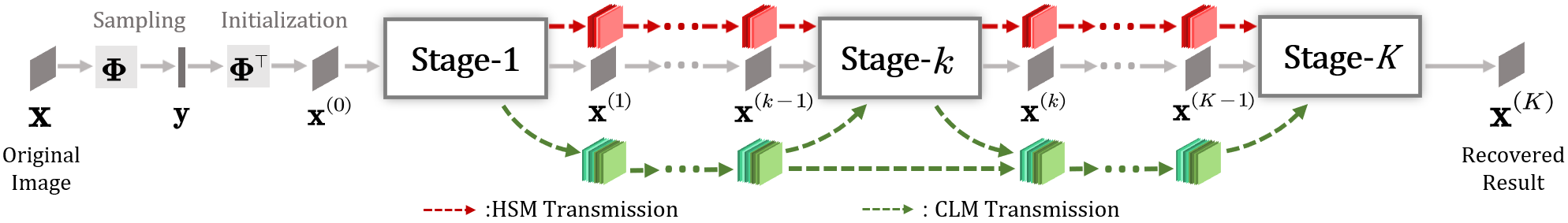
Figure 1. Architecture of our proposed MADUN, which consists of $K$ stages. $\mathbf{x}$ denotes the full-sampled image for training, $\mathbf{\Phi}$ denotes measurement matrix, $\mathbf{y}$ is the under-sampled data, $\mathbf{x}^{(0)}$ denotes the initialization, $\mathbf{x}^{(K)}$ denotes the recovered result of MADUN and $\mathbf{x}^{(k)}$ stands for the output images of ($k$)-th stage. The dotted red line denotes High-throughput Short-term Memory (HSM) transmission and the dotted green line denotes Cross-stage Long-term Memory (CLM) transmission.

Recently, fueled by the powerful learning ability of deep networks, several deep network-based image CS reconstruction algorithms have been proposed (Kulkarni et al., 2016)(Sun et al., 2020)(Gilton et al., 2019)(Chen et al., 2020), which can be generally grouped into two categories: deep non-unfolding networks (DNUNs) and deep unfolding networks (DUNs). For DNUN, it aims to directly learn the inverse mapping from the CS measurement domain to the original signal domain (Mousavi et al., 2015)(Iliadis et al., 2018). For DUN, it combines deep network with optimization and trains a truncated unfolding inference through an end-to-end learning process (Zhang and Ghanem, 2018)(Zhang et al., 2020c)(You et al., 2021a)(You et al., 2021b), which has become the mainstream for CS.

DUN is usually composed of a fixed number of stages where each stage is mainly influenced by its direct former one, and the mechanism can be considered as short-term memory, e.g., ISTA-Net (Zhang and Ghanem, 2018) and DPDNN (Zhang et al., 2020a). In each stage, the information transmission is usually hampered by the feature transformation with channel number reduction from multiple to one. Besides, the information in the prior stages is easily forgotten and the long-term dependency problem is rarely realized, which causes inadequate recoveries.

To address the above issues, in this paper, we propose a Memory-Augmented Deep Unfolding Network (MADUN), focusing on CS reconstruction. In our MADUN, we design a Memory-Augmented Proximal Mapping Module (MAPMM) which contains two different memory augmentation mechanisms, as shown in Figure 1. To reduce information loss between each two adjacent stages, we design a High-throughput Short-term Memory mechanism (HSM) to adaptively add multi-channel information and well ensure maximum signal flow. Also, a Cross-stage Long-term Memory mechanism (CLM) is exploited to explicitly construct the deep and adjustable long-term information path across stages. Our MADUN is a comprehensive framework, considering the merits of previous optimization-inspired DUNs and meanwhile, improving the network representation ability by augmenting entire information transmission among all stages. It enjoys the advantages of both the satisfaction of interpretability and the ensurance of information abundance. The major contributions are summarized as follows:

• We propose a novel Memory-Augmented Deep Unfolding Network (MADUN) with persistent memory for CS reconstruction, which is able to adaptively capture the adequate features and recover more details and textures.

• We design a Memory-Augmented Proximal Mapping Module (MAPMM) to enhance information transmission, which contains two different memory augmentation mechanisms.

• We introduce a High-throughput Short-term Memory mechanism (HSM) which is exploited to allow MADUN to transmit high-throughput information between adjacent stages.

• We also develop a Cross-stage Long-term Memory mechanism (CLM) to explore the long-term dependency of deep information across all cascading stages.

• Extensive experiments show that, with the strong ability of the balance between the short-term and the long-term memories, our MADUN outperforms existing state-of-the-art networks by large margins.

2. related work

2.1. Deep Non-Unfolding Network

Deep non-unfolding network (DNUN) directly learns mapping functions from the CS sampling image $\mathbf{\Phi}\mathbf{x}$ to the full-sampled image $\mathbf{x}$, resulting in an end-to-end network. Kulkarni et al. (Kulkarni et al., 2016) develop a CNN-based CS algorithm, dubbed ReconNet, which learns to regress an image block from its CS measurement. Sun et al. (Sun et al., 2020) design a dual-path network to learn the structure-texture decomposition in a data-driven manner. Residual learning and U-Net structure are adopted in CS-MRI to successfully learn the aliasing artifacts (Hyun et al., 2018). Some works jointly learn the measurement by a sampling sub-network and the recovery by a reconstruction sub-network from the training data. CSNet (Shi et al., 2019a) can avoid blocking artifacts by learning an end-to-end mapping between measurements and the whole reconstructed images. Shi et al. (Shi et al., 2019b) exploit a convolutional neural network for scalable sampling and quality scalable reconstruction.

Apparently compared with traditional methods, DNUNs can represent image information flexibly with the fast inferencing efficiency. However, in DNUNs, the learning performance seriously depends on the careful tuning and the sampling matrix is not well-embedded in the reconstruction process, which not only result in the very tricky training schemes but also drag down the network performance due to the difficulty of directly learning the recovery mapping without explicit matrix guidance.

2.2. Deep Unfolding Network

Deep unfolding networks (DUNs) have been proposed to solve different image inverse tasks, such as denoising (Chen and Pock, 2016)(Lefkimmiatis, 2017), deblurring (Kruse et al., 2017)(Wang et al., 2020), and demosaicking (Kokkinos and Lefkimmiatis, 2018). DUN has friendly interpretability on training data pairs $\{(\mathbf{y}_{j},\mathbf{x}_{j})\}_{j=1}^{N_{a}}$, which is usually formulated on CS construction as the bi-level optimization problem:

(2) $$\begin{aligned} &\underset{\Theta}{\min}\sum_{j=1}^{N_{a}}{\mathcal{L}(\mathbf{\hat{x}}_{j},\mathbf{x}_{j})},\\ &\mathbf{s.t.}\ \mathbf{\hat{x}}_{j}=\underset{\mathbf{x}}{\arg\min}\frac{1}{2}||\mathbf{\Phi}\mathbf{x}-\mathbf{y}_{j}||_{2}^{2}+\lambda\mathcal{F}(\mathbf{x}).\end{aligned}$$

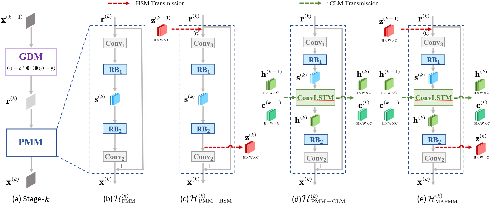
Figure 2. (a) is the illustration of ($k$)-th stage in MADUN, where $\mathbf{r}^{(k)}$ is the outputs of the Gradient Descent Module (GDM) and the inputs of the Proximal Mapping Module (PMM). (b) is the PMM. (c) is the PMM with High-throughput Short-term Memory (HSM). (d) is the PMM with Cross-stage Long-term Memory (CLM). (e) is our proposed Memory-Augmented Proximal Mapping Module (MAPMM) which combines HSM and CLM with PMM. Here, “+” is a residual learning strategy, “$\copyright$” is the concatenation along channel dimension, $H$ and $W$ denote the height and width of the image and $C$ is the filter number.

DUNs on CS and compressive sensing MRI (CS-MRI) usually integrate some effective convolutional neural network (CNN) denoisers into some optimization methods including half quadratic splitting (HQS) (Zhang et al., 2017b)(Dong et al., 2018)(Aggarwal et al., 2018), alternating minimization (AM) (Schlemper et al., 2017)(Sun et al., 2018)(Zheng et al., 2019), iterative shrinkage-thresholding algorithm (ISTA) (Zhang and Ghanem, 2018)(Gilton et al., 2019)(Zhang et al., 2020c), approximate message passing (AMP) (Zhang et al., 2020b)(Zhou et al., 2020), alternating direction method of multipliers (ADMM) (Yang et al., 2018) and inertial proximal algorithm for nonconvex optimization (iPiano) (Su and Lian, 2020). Different optimization methods usually lead to different optimization-inspired DUNs.

Although existing DUNs inherit a good structure from optimization and exhibit friendly interpretability, we find that, from the perspective of neural networks, DUNs’ inherent design of taking one-channel images as inputs and outputs for each stage will greatly hinder network information transmission and lose much more image details. Chen et al. (Chen et al., 2020) propose a contextual memory (CM) module which can augment the sequential links across stages. However, the CM module is still hard to maintain abundant details due to the poor storage capacity of one-channel stage outputs.

3. Proposed Method

In this section, we will elaborate on the design of our proposed Memory-Augmented Deep Unfolding Network (MADUN) for CS.

3.1. Basic Network Architecture

As we all know, DUN is a kind of CNN method that combines an efficient iterative algorithm. Iterative shrinkage-thresholding algorithm (ISTA) is well suited for solving many large-scale linear inverse problems (Zhang and Ghanem, 2018), e.g., general CS and CS-MRI. Traditional ISTA solves the CS reconstruction problem in Eq. (1) by iterating between the following update steps:

(3) $$\mathbf{r}^{(k)}=\mathbf{x}^{(k-1)}-\rho\mathbf{\Phi^{\top}}\left(\mathbf{\Phi}\mathbf{x}^{(k-1)}-\mathbf{{y}}\right),$$

(4) $$\mathbf{x}^{(k)}=\underset{\mathbf{x}}{\arg\min}\frac{1}{2}||\mathbf{x}-\mathbf{r}^{(k)}||_{2}^{2}+\lambda\mathcal{F}(\mathbf{x}),$$

where $\rho$ is the step size. Inspired by ISTA-Net ⁺ (Zhang and Ghanem, 2018) which is a DUN unfolded by ISTA, Eq. (3) and Eq. (4) can be expressed as two modules in the ($k$)-th stage $\leavevmode\nobreak\ (0<k\leq K)$ as shown in Figure 2 (a):

(5) $$\mathbf{r}^{(k)}=\mathbf{x}^{(k-1)}-\rho^{(k)}\mathbf{\Phi^{\top}}\left(\mathbf{\Phi}\mathbf{x}^{(k-1)}-\mathbf{{y}}\right),$$

(6) $$\mathbf{x}^{(k)}=\displaystyle{\mathcal{H}}_{\scriptscriptstyle{\operatorname{PMM}}}^{(k)}(\mathbf{r}^{(k)}).$$

Eq. (5) is called gradient descent module (GDM) where $\rho^{(k)}$ is a learnable parameter, and Eq. (6) is called proximal mapping module (PMM) which is actually a CNN-based denoiser.

To keep a simple structure with the high recovery accuracy, PMM uses basic convolution layers (Conv) and residual blocks (RB) which generate residual outputs by the structure of Conv-ReLU-Conv, and adopts an efficient reconstruction network (Zhang et al., 2017a) as shown in Figure 2 (b), which can be divided into four parts:

• A convolution layer receives one-channel network inputs $\mathbf{r}^{(k)}$ and generates multi-channel outputs, yielding $\operatorname{Conv_{1}}(\mathbf{r}^{(k)})$.

• A mapping layer extracts deep representation, which consists of two residual blocks ($\operatorname{RB_{1}}(\cdot)$ and $\operatorname{RB_{2}}(\cdot)$) in PMM due to optimizing easily (He et al., 2016). Here, $\mathbf{s}^{(k)}$ is the intermediate result produced between the two residual blocks.

• A convolution layer $\operatorname{Conv_{2}}(\cdot)$ outputs residual result by the feature conversions from multi-channel to one-channel.

• A residual learning strategy produces final module outputs.

Accordingly, PMM can be formulated $\mathbf{x}^{(k)}=\displaystyle{\mathcal{H}}_{\scriptscriptstyle{\operatorname{PMM}}}^{(k)}(\mathbf{r}^{(k)})$ as:

(7) $$\mathbf{x}^{(k)}=\mathbf{r}^{(k)}+\operatorname{Conv_{2}}(\operatorname{RB_{2}}(\operatorname{RB_{1}}(\operatorname{Conv_{1}}(\mathbf{r}^{(k)})))).$$

3.2. Memory-Augmented DUN

Motivated by the viewpoint that the human brain achieves memory by preserving and storing what they acquire or are informed previously (Cichon and Gan, 2015), the information flow across stages can also be regarded as short-term memory transmission in DUNs, where $\mathbf{x}^{(k)}$ in Figure 2 is as the link between each two adjacent stages. However, $\operatorname{Conv_{2}}(\cdot)$ in Eq. (7) is a lossy conversion process which would cause memory loss. Here, we propose a Memory-Augmented Deep Unfolding Network (MADUN) which augments memory across stages, each of which shares a unified two-step recovering scheme as follows:

(8) $$\mathbf{r}^{(k)}=\displaystyle{\mathcal{H}}_{\scriptscriptstyle{\operatorname{GDM}}}^{(k)}(\mathbf{x}^{(k-1)}),$$

(9) $$\mathbf{x}^{(k)}=\displaystyle{\mathcal{H}}_{\scriptscriptstyle{\operatorname{MAPMM}}}^{(k)}(\mathbf{r}^{(k)}).$$

Here, GDM is trivial (Zhang and Ghanem, 2018) and is the same as Eq. (3), and Memory-Augmented Proximal-Mapping Module (MAPMM) is introduced with two types of memory augmentation mechanisms which can highly strengthen the information transmission among all stages.

3.3. Memory-Augmented Proximal Mapping

On the basis of PMM, MAPMM introduces High-throughput Short-term Memory (HSM) and Cross-stage Long-term Memory (CLM), which greatly enhance the network representation capability.

3.3.1. High-throughput Short-term Memory (HSM)

To address the information-lossy intra-stage transmission, we introduce HSM with multi-channel $\mathbf{z}^{(k-1)}$ (of size $H\times W\times C$) to bridge a high-capacity path between adjacent stages. As shown in Figure 2 (c) and as the output of $\operatorname{RB_{2}}(\cdot)$ at $(k-1)$-th stage, $\mathbf{z}^{(k-1)}$ is:

(10) $$\mathbf{z}^{(k-1)}=\operatorname{RB_{2}}(\mathbf{s}^{(k-1)}).$$

Concatenating $\mathbf{z}^{(k-1)}$ with $\mathbf{r}^{(k)}$ followed by $\operatorname{Conv_{3}}(\cdot)$ generates $C$-channel features. The remaining process is the same with Eq. (7). Thus, PMM with HSM, denoted by $\mathbf{x}^{(k)}=\displaystyle{\mathcal{H}}_{\scriptscriptstyle{\operatorname{PMM-HSM}}}^{(k)}(\mathbf{r}^{(k)})$, is:

(11) $$\mathbf{x}^{(k)}=\mathbf{r}^{(k)}+\operatorname{Conv_{2}}(\operatorname{RB_{2}}(\operatorname{RB_{1}}(\operatorname{Conv_{3}}(\mathbf{r}^{(k)}\|\mathbf{z}^{(k-1)})))),$$

where $\|$ denotes concatenating the feature maps. Obviously, $\mathbf{z}^{(k-1)}$ transmits high-throughput information from the previous stage to the current stage, achieving multi-channel short-term memory which ensures maximum flow and reduces information loss caused by the conventional channel-shrinking transformation.

3.3.2. Cross-stage Long-term Memory (CLM)

For modeling explicitly the long-range dependencies among all cascading stages, we utilize a ConvLSTM layer (Shi et al., 2015), which has been well-validated to be a stable and powerful way to balance the past and current states, to develop the cross-stage long-term memory (CLM) and further enhance the signal conversion and transmission.

In the process of achieving CLM, the ConvLSTM layer is sandwiched between two residual blocks ($\operatorname{RB_{1}}(\cdot)$ and $\operatorname{RB_{2}}(\cdot)$), and updates cell outputs $\mathbf{c}^{(k)}$ and hidden states $\mathbf{h}^{(k)}$ with the inputs of the intermediate result $\mathbf{s}^{(k)}=\operatorname{RB_{1}}(\operatorname{Conv_{1}}(\mathbf{r}^{(k)}))$ in Figure 2 (d),

(12) $$[\mathbf{h}^{(k)},\mathbf{c}^{(k)}]=\operatorname{ConvLSTM}(\mathbf{s}^{(k)},[\mathbf{h}^{(k-1)},\mathbf{c}^{(k-1)}]),$$

where CLM $[\mathbf{h}^{(k-1)}$, $\mathbf{c}^{(k-1)}]$ updates the current state of deep information, predicts multi-stage information and achieves long-term memory across cascading stages. The architecture of ConvLSTM with inputs $\mathbf{s}^{(k)}$ can be expressed as:

(13) $$\mathbf{i}^{(k)} =\sigma({\emph{W}_{si}}\ast\mathbf{s}^{(k)}+{\emph{W}_{hi}}\ast\mathbf{h}^{(k-1)}+\emph{b}_{i}),$$

$$\mathbf{f}^{(k)} =\sigma({\emph{W}_{sf}}\ast\mathbf{s}^{(k)}+{\emph{W}_{hf}}\ast\mathbf{h}^{(k-1)}+\emph{b}_{f}),$$

$$\mathbf{c}^{(k)} =\mathbf{f}^{(k)}\circ\mathbf{c}^{(k-1)}+\mathbf{i}^{(k)}\circ\operatorname{tanh}({\emph{W}_{sc}}\ast\mathbf{s}^{(k)}+{\emph{W}_{hc}}\ast\mathbf{h}^{(k-1)}+\emph{b}_{c}),$$

$$\mathbf{o}^{(k)} =\sigma({\emph{W}_{so}}\ast\mathbf{s}^{(k)}+{\emph{W}_{ho}}\ast\mathbf{h}^{(k-1)}+\emph{b}_{o}),$$

$$\mathbf{h}^{(k)} =\mathbf{o}^{(k)}\circ\operatorname{tanh}(\mathbf{c}^{(k)}),$$

where $\ast$ denotes the convolution operator, $\circ$ denotes the Hadamard product, $\emph{W}_{si},\emph{W}_{hi},\ldots,\emph{W}_{ho}$ are the filter weights, $\emph{b}_{i},\emph{b}_{f},\ldots,\emph{b}_{o}$ are the bias, $\mathbf{i}^{(k)}$, $\mathbf{f}^{(k)},\mathbf{o}^{(k)}$ denote the input gate, the forget gate and the output gate respectively, $\sigma(\cdot)$ and $\operatorname{tanh}(\cdot)$ denote the sigmoid function and the tanh function respectively. $\mathbf{c}^{(k)}$ acts as an accumulator of the state information and $\mathbf{h}^{(k)}$ is further controlled by the lastest cell outputs $\mathbf{c}^{(k)}$ and the output gate $\mathbf{o}^{(k)}$.

$\mathbf{h}^{(k)}$ is directly utilized as the inputs of $\operatorname{RB_{2}}(\cdot)$ in the current stage and $[\mathbf{h}^{(k)}$, $\mathbf{c}^{(k)}]$ transmits deep features at the same position across stages to augment the dependency of deep information. And the rest process of achieving CLM in PMM is the same with Eq. (7). So the process of $\mathbf{x}^{(k)}=\displaystyle{\mathcal{H}}_{\scriptscriptstyle{\operatorname{PMM-CLM}}}^{(k)}(\mathbf{r}^{(k)})$ can be reformulated as:

(14) $$\mathbf{x}^{(k)}=\mathbf{r}^{(k)}+\operatorname{Conv_{2}}(\operatorname{RB_{2}}(\operatorname{ConvLSTM}(\operatorname{RB_{1}}(\operatorname{Conv_{1}}(\mathbf{r}^{(k)}))))).$$

Therefore, incorporating both HSM $\mathbf{z}^{(k-1)}$ and CLM $[\mathbf{h}^{(k-1)},\\ \mathbf{c}^{(k-1)}]$ into PMM and with the inputs $\mathbf{r}^{(k)}$ in the ($k$)-th stage, the proposed memory-augmented proximal mapping module (MAPMM) in Figure 2 (e), denoted by $\mathbf{x}^{(k)}=\displaystyle{\mathcal{H}}_{\scriptscriptstyle{\operatorname{MAPMM}}}^{(k)}(\mathbf{r}^{(k)})$ is formulated as:

(15) $$\mathbf{x}^{(k)}=\mathbf{r}^{(k)}+\operatorname{Conv_{2}}(\operatorname{RB_{2}}(\operatorname{ConvLSTM}(\operatorname{RB_{1}}(\operatorname{Conv_{3}}(\mathbf{r}^{(k)}\|\mathbf{z}^{(k-1)}))))).$$

Comparing Eq. (15) with Eq. (7), it is obvious to observe that $\mathbf{z}^{(k-1)}$ is able to effectively add high-throughput information between each two adjacent stages, while $[\mathbf{h}^{(k-1)},\mathbf{c}^{(k-1)}]$ can augment mid/
high-frequency information by applying ConvLSTM layers across cascading stages. Therefore, our proposed MAPMM enhances information transmission among all stages by adaptively learning these two types of memory mechanisms.

3.4. Initialization of HSM and CLM

Given the measurements $\mathbf{y}$ as the known information, HSM $\mathbf{z}^{(k)}$ is initialized by applying a light-weight one-convolution layer $\operatorname{Conv_{0}}(\cdot)$ on the image $\mathbf{\Phi^{\top}}\mathbf{y}$ to generate $C$ feature maps, yielding:

(16) $$\mathbf{z}^{(0)}=\operatorname{Conv_{0}}(\mathbf{\Phi^{\top}}\mathbf{y}).$$

Considering that CLM $[\mathbf{h}^{(k)}$, $\mathbf{c}^{(k)}]$ has its physical meaning and it is practical to assume no prior knowledge is used at the beginning, therefore, we simply initialize $[\mathbf{h}^{(k)}$, $\mathbf{c}^{(k)}]$ to be zero.

3.5. Network Parameters and Loss Function

The learnable parameter set in MADUN, denoted by $\boldsymbol{\Theta}$, can be expressed as $\boldsymbol{\Theta}=\{\operatorname{Conv_{0}}(\cdot)\}\bigcup\{\rho^{(k)},\displaystyle{\mathcal{H}}_{\scriptscriptstyle{\operatorname{MAPMM}}}^{(k)}(\cdot)\}_{k=1}^{K}$. $\operatorname{Conv_{0}}(\cdot)$ is a one-convolution layer with one input channel and $C$ output channels. $\displaystyle{\mathcal{H}}_{\scriptscriptstyle{\operatorname{MAPMM}}}^{(k)}(\cdot)$ consists of $\operatorname{Conv_{3}}(\cdot)$, $\operatorname{Conv_{2}}(\cdot)$, $\operatorname{RB_{1}}(\cdot)$, $\operatorname{RB_{2}}(\cdot)$ and $\operatorname{ConvLSTM}(\cdot)$ whose parameters are different in each stage. $\operatorname{Conv_{3}}(\cdot)$ with $C+1$ input channels and $C$ output channels receives networks inputs, and $\operatorname{Conv_{2}}(\cdot)$ with $C$ input channels and one output channel outputs residual results. Also, the parameters of $\operatorname{RB_{1}}(\cdot)$ and $\operatorname{RB_{2}}(\cdot)$ are both from two convolution layers without the change of the channel number (with $C$ input channels and $C$ output channels), while $\operatorname{ConvLSTM}(\cdot)$ is same with (Li et al., 2018). Here, all the convolutions in MADUN adopt $3\times 3$ filter kernels.

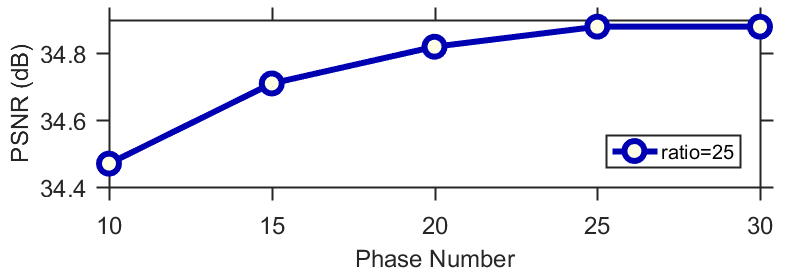
Figure 3. Average PSNR curve by MADUN on Set11 dataset with various stage numbers. When stage number is 25, the curve begins to reach peak performance.

Table 1. Ablation study on effects of components at ratio=$10\%$. $\ast$HSM and $\circ$HSM represent the different positions of linking memory. The best performance is labeled in bold.

Cases	$\ast$HSM	$\circ$HSM	HSM	CLM	PSNR/SSIM
					Set11	Urban100
(a)	-	-	-	-	28.66/0.8609	25.77/0.7905
(b)	-	-	-	$\surd$	29.24/0.8760	26.68/0.8282
(c)	$\surd$	-	-	-	29.06/0.8713	26.46/0.8207
(d)	-	$\surd$	-	-	29.32/0.8770	26.88/0.8263
(e)	-	-	$\surd$	-	29.35/0.8786	26.94/0.8305
(f)	-	-	$\surd$	$\surd$	29.44/0.8807	27.13/0.8393

Given a set of full-sampled images $\left\{\mathbf{x}_{j}\right\}_{j=1}^{N_{a}}$ and some sampling patterns with CS ratio $\gamma$, the under-sampled $k$-space data is obtained by $\mathbf{y}_{j}=\mathbf{\Phi}\mathbf{x}_{j}$, producing the train data pairs $\{(\mathbf{y}_{j},\mathbf{x}_{j})\}_{j=1}^{N_{a}}$. Our MADUN takes $\mathbf{y}_{j}$ as inputs and generates the reconstruction result $\mathbf{x}_{j}^{(K)}$ as outputs with the initialization $\mathbf{x}_{j}^{(0)}=\mathbf{\Phi^{\top}}\mathbf{y}_{j}$. The loss function is designed to use $L_{1}$ loss between $\mathbf{x}_{j}$ and $\mathbf{x}_{j}^{(K)}$ as:

(17) $$\mathcal{L}(\boldsymbol{\Theta})=\ \frac{1}{{N}{N_{a}}}\sum_{j=1}^{N_{a}}{\left\|\mathbf{x}_{j}-\mathbf{x}_{j}^{(K)}\right\|}_{1},$$

where $N_{a}$, $N$ and $K$ represent the number of training images, the size of each image and the stage number of MADUN respectively.

4. experiment

4.1. Implementation Details

We use the 400 training images of size $180\times 180$ (Chen and Pock, 2016), generating the training data pairs $\{(\mathbf{y}_{j},\mathbf{x}_{j})\}_{j=1}^{N_{a}}$ by extracting the luminance component of each image block of size $33\times 33$, i.e. $N=1,089$. Meanwhile, we apply in the data augmentation technique to increase the data diversity. For a given CS ratio, the corresponding measurement matrix $\mathbf{\Phi}\in\mathbb{R}^{M\times N}$ is constructed by generating a random Gaussian matrix or a jointly learned matrix and then orthogonalizing its rows, i.e. $\mathbf{\Phi}\mathbf{\Phi^{\top}}=\mathbf{I}$, where $\mathbf{I}$ is the identity matrix. Applying $\mathbf{y}_{j}=\mathbf{\Phi}\mathbf{x}_{j}$ yields the set of CS measurements, where $\mathbf{x}_{j}$ is the vectorized version of an image block.

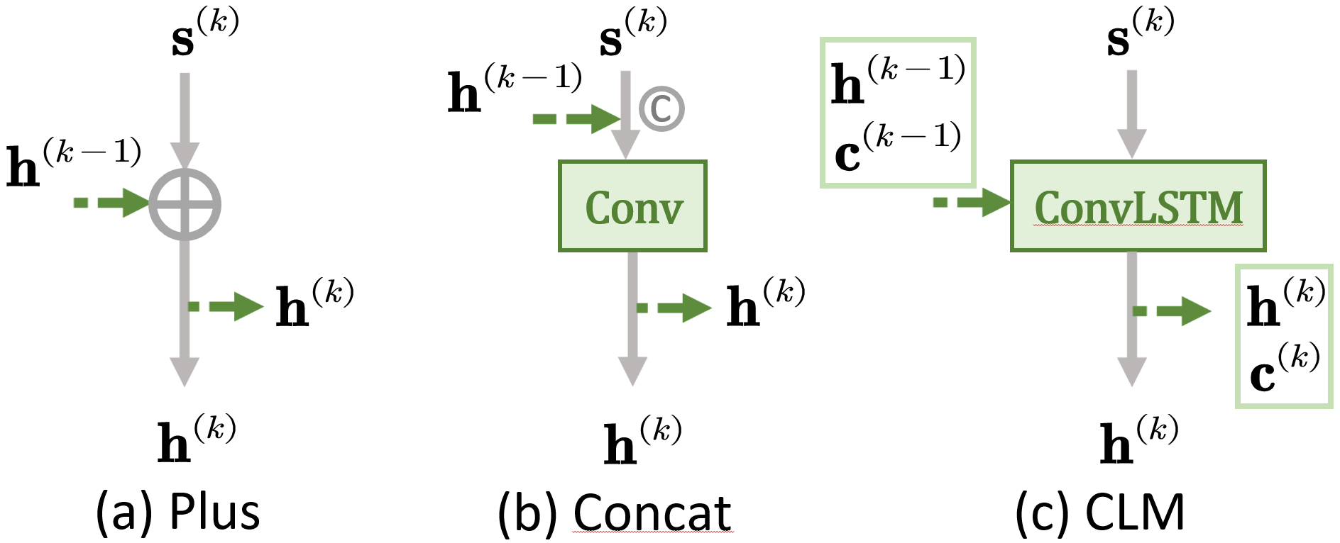
Figure 4. Illustration of three different methods achieving memory across stages, corresponding to Table 2.

Table 2. Ablation study on the effect of CLM. Average PSNR/SSIM at ratio=$10\%,25\%,30\%$ on Set11 dataset. The best performance is labeled in bold.

Methods	Plus	Concat	CLM
10%	28.83/0.8659	29.10/0.8733	29.24/0.8760
25%	34.33/0.9446	34.54/0.9465	34.69/0.9480
30%	35.62/0.9547	35.74/0.9560	35.93/0.9570

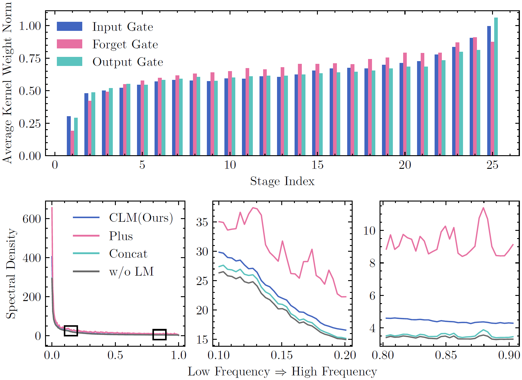
Figure 5. Illustration of the average kernel weight norm in each stage (upper) and the 1-D spectral density curves of different CLM variants (lower).

Table 3. Average PSNR/SSIM performance comparisons on Set11, CBSD68 and Urban100 datasets with different CS ratios. We compare MADUN with two DNUNs and six DUNs with fixed random gaussian matrix. The best and second best results are highlighted in red and blue colors, respectively.

Dataset	Methods	CS Ratio
		10%	25%	30%	40%	50%
	ReconNet (Kulkarni et al., 2016)	23.96/0.7172	26.38/0.7883	28.20/0.8424	30.02/0.8837	30.62/0.8983
	DPA-Net (Sun et al., 2020)	27.66/0.8530	32.38/0.9311	33.35/0.9425	35.21/0.9580	36.80/0.9685
	IRCNN (Zhang et al., 2017b)	23.05/0.6789	28.42/0.8382	29.55/0.8606	31.30/0.8898	32.59/0.9075
	ISTA-Net+ (Zhang and Ghanem, 2018)	26.58/0.8066	32.48/0.9242	33.81/0.9393	36.04/0.9581	38.06/0.9706
	DPDNN (Dong et al., 2018)	26.23/0.7992	31.71/0.9153	33.16/0.9338	35.29/0.9534	37.63/0.9693
Set11	GDN (Gilton et al., 2019)	23.90/0.6927	29.20/0.8600	30.26/0.8833	32.31/0.9137	33.31/0.9285
	MAC-Net (Chen et al., 2020)	27.68/0.8182	32.91/0.9244	33.96/0.9372	35.94/0.9560	37.67/0.9668
	iPiano-Net (Su and Lian, 2020)	28.05/0.8460	33.53/0.9359	34.78/0.9472	37.01/0.9631	38.94/0.9737
7
	MADUN	29.44/0.8807	34.88/0.9496	36.07/0.9582	38.13/0.9700	39.92/0.9779
	ReconNet (Kulkarni et al., 2016)	24.02/0.6414	26.01/0.7498	27.20/0.7909	28.71/0.8409	29.32/0.8642
	DPA-Net (Sun et al., 2020)	25.47/0.7372	29.01/0.8595	29.73/0.8827	31.17/0.9156	32.55/0.9386
	IRCNN (Zhang et al., 2017b)	23.07/0.5580	26.44/0.7206	27.31/0.7543	28.76/0.8042	30.00/0.8398
	ISTA-Net+ (Zhang and Ghanem, 2018)	25.37/0.7022	29.32/0.8515	30.37/0.8786	32.23/0.9165	34.04/0.9425
	DPDNN (Dong et al., 2018)	25.35/0.7020	29.28/0.8513	30.39/0.8807	32.21/0.9171	34.27/0.9455
CBSD68	GDN (Gilton et al., 2019)	23.41/0.6011	27.11/0.7636	27.52/0.7745	30.14/0.8649	30.88/0.8763
	MAC-Net (Chen et al., 2020)	25.80/0.7024	29.42/0.8469	30.28/0.8713	32.02/0.9085	33.68/0.9352
	iPiano-Net (Su and Lian, 2020)	26.34/0.7431	30.16/0.8711	31.24/0.8964	33.14/0.9298	34.98/0.9521
7
	MADUN	26.83/0.7620	30.81/0.8844	31.87/0.9068	33.81/0.9376	35.82/0.9587
	ReconNet (Kulkarni et al., 2016)	21.49/0.6223	23.31/0.7107	24.72/0.7697	26.44/0.8250	27.06/0.8447
	DPA-Net (Sun et al., 2020)	24.55/0.7841	28.80/0.8944	29.47/0.9034	31.09/0.9311	32.08/0.9447
	IRCNN (Zhang et al., 2017b)	21.62/0.6137	26.38/0.7955	27.47/0.8248	29.22/0.8645	30.63/0.8900
	ISTA-Net+ (Zhang and Ghanem, 2018)	23.61/0.7238	28.93/0.8840	30.21/0.9079	32.43/0.9377	34.43/0.9571
	DPDNN (Dong et al., 2018)	23.69/0.7211	28.70/0.8798	30.06/0.9005	32.27/0.9350	34.81/0.9579
Urban100	GDN (Gilton et al., 2019)	21.48/0.5958	25.75/0.7704	26.72/0.7950	28.96/0.8698	29.89/0.8768
	MAC-Net (Chen et al., 2020)	24.21/0.7445	28.79/0.8798	29.99/0.9017	31.94/0.9272	34.03/0.9513
	iPiano-Net (Su and Lian, 2020)	25.67/0.7963	30.87/0.9157	32.16/0.9320	34.27/0.9531	36.22/0.9675
7
	MADUN	27.13/0.8393	32.54/0.9347	33.77/0.9472	35.80/0.9633	37.75/0.9746

To train the network, we use Adam optimization (Kingma and Ba, 2015) with a learning rate of 0.0001, and a batch size of 64. We also use momentum of 0.9 and weight decay of 0.999. For MADUN, the models are trained with 410 epochs separately for each CS ratio. Each image block of size $33\times 33$ is sampled and reconstructed independently for the first 400 epochs, and for the last ten epochs, we adopt larger image blocks of size $99\times 99$ as inputs to further fine-tune the model. To alleviate blocking artifacts, we firstly unfold the blocks of size $99\times 99$ into overlapping blocks of size $33\times 33$ while sampling process $\mathbf{\Phi}\mathbf{x}$ and then fold the blocks of size $33\times 33$ into larger blocks while initialization $\mathbf{\Phi^{\top}}\mathbf{y}$ (Su and Lian, 2020). We also unfold the whole image with this approach during testing. The default stage number $K$ is set to be 25 and the default number of feature maps $C$ is set to be 32. And the learnable parameters $\rho^{(k)}$ is initialized to 1. The CS reconstruction accuracies on the all datasets are evaluated with PSNR and SSIM.

4.2. Ablation Study

4.2.1. Performance Effect of Stage Number

The average PSNR curve in Figure 3 is the results when ratio is $25\%$ on Set11 dataset. To get a better trade-off between model performance and complexity, we choose $K=25$ as the default setting in all experiments.

4.2.2. Performance Effect of MADUN Components

Based on the PMM structure, we do ablation experiments on the HSM and CLM at ratio=$10\%$ on Set11 and Urban100 dataset, as shown in Table 1. To demonstrate the effectiveness of HSM and CLM, we removes them from MADUN to form two simplified versions, corresponding to Figure 2 (c) and Figure 2 (d) respectively. We conclude that they are all effective ways to compensate the signal flow among stages, and HSM plays a more important role by bridging each two adjacent stages with a high-throughput short-term transmission.

4.3. Analysis of Memory Augmentation

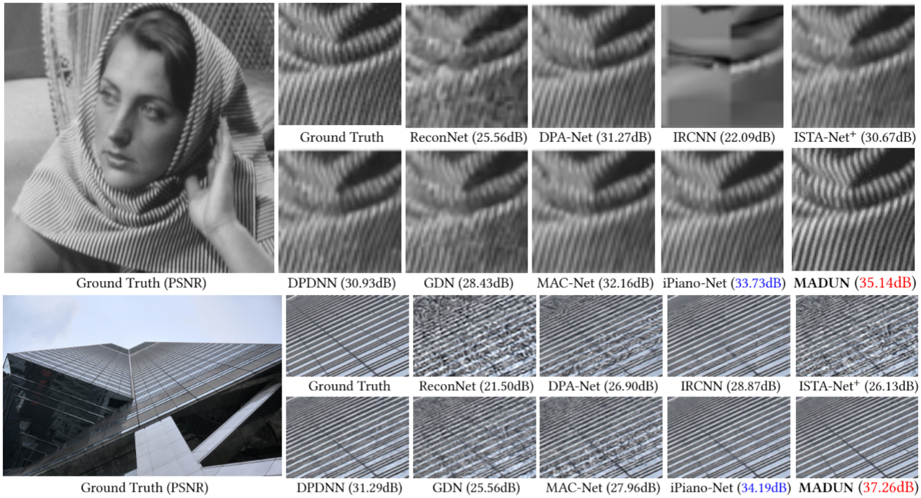
Figure 6. Comparisons on recovering an image named “Barbara” from Set11 dataset in the case of CS ratio = 30% (upper) and an image from Urban100 dataset in the case of CS ratio = 40% (lower).

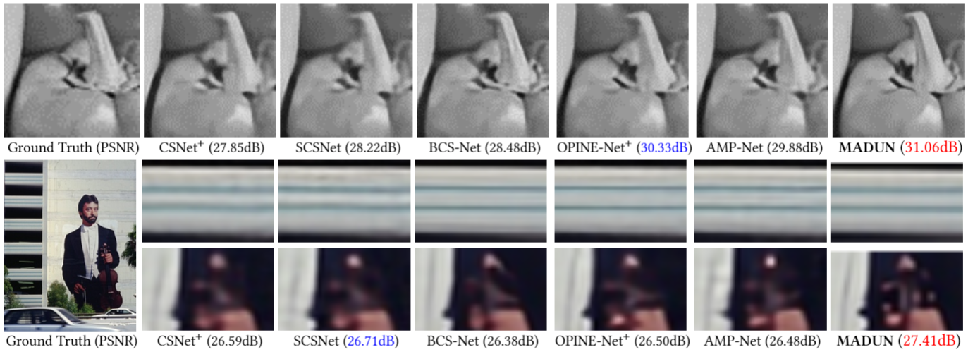
Figure 7. Comparisons on recovering an image named “Peppers” from Set11 dataset (upper) and an image from CBSD68 dataset (lower) in the case of CS ratio = 10%.

Table 4. Average PSNR/SSIM performance comparisons on Set11 and CBSD68 datasets with different CS ratios. We compare MADUN with two DNUNs and three DUNs with jontly learning the sampling matrix and the reconstruction process.

Dataset	Methods	CS Ratio
		10%	25%	30%	40%	50%
Set11	CSNet+(Shi et al., 2019a)	28.34/0.8580	33.34/0.9387	34.27/0.9492	36.44/0.9690	38.47/0.9796
	SCSNet (Shi et al., 2019b)	28.52/0.8616	33.43/0.9373	34.64/0.9511	36.92/0.9666	39.01/0.9769
	BCS-Net (Zhou et al., 2020)	29.42/0.8673	34.20/0.9408	35.63/0.9495	36.68/0.9667	39.58/0.9734
	OPINE-Net+(Zhang et al., 2020c)	29.81/0.8904	34.86/0.9509	35.79/0.9541	37.96/0.9633	40.19/0.9800
	AMP-Net (Zhang et al., 2020b)	29.42/0.8782	34.60/0.9469	35.91/0.9576	38.25/0.9714	40.26/0.9786
7
	MADUN	29.91/0.8986	35.66/0.9601	36.94/0.9676	39.15/0.9772	40.77/0.9832
CBSD68	CSNet+(Shi et al., 2019a)	27.91/0.7938	31.12/0.9060	32.20/0.9220	35.01/0.9258	36.76/0.9638
	SCSNet (Shi et al., 2019b)	28.02/0.8042	31.15/0.9058	32.64/0.9237	35.03/0.9214	36.27/0.9593
	BCS-Net (Zhou et al., 2020)	27.98/0.8015	31.29/0.8846	32.70/0.9301	35.14/0.9397	36.85/0.9682
	OPINE-Net+(Zhang et al., 2020c)	27.82/0.8045	31.51/0.9061	32.35/0.9215	34.95/0.9261	36.35/0.9660
	AMP-Net (Zhang et al., 2020b)	27.79/0.7853	31.37/0.8749	32.68/0.9291	35.06/0.9395	36.59/0.9620
7
	MADUN	28.15/0.8229	32.26/0.9221	33.35/0.9379	35.42/0.9606	37.11/0.9730

Table 5. Average PSNR/SSIM performance comparisons on testing brain MR images with one DNUN and six DUNs.

CS Ratio	Hyun et al. (Hyun et al., 2018)	Schlemper et al. (Schlemper et al., 2017)	ADMM-Net (Yang et al., 2018)	RDN (Sun et al., 2018)	CDDN (Zheng et al., 2019)	ISTA-Net+ (Zhang and Ghanem, 2018)	MoDL (Aggarwal et al., 2018)	MADUN
10%	32.78/0.8385	34.23/0.8921	34.42/0.8971	34.59/0.8968	34.63/0.9002	34.65/0.9038	35.18/0.9091	36.15/0.9237
20%	36.36/0.9070	38.47/0.9457	38.60/0.9478	38.58/0.9470	38.59/0.9474	38.67/0.9480	38.51/0.9457	39.44/0.9542
30%	38.85/0.9383	40.85/0.9628	40.87/0.9633	40.82/0.9625	40.89/0.9633	40.91/0.9631	40.97/0.9636	41.48/0.9666
40%	40.65/0.9539	42.63/0.9724	42.58/0.9726	42.64/0.9723	42.59/0.9725	42.65/0.9727	42.38/0.9705	43.06/0.9746
50%	42.35/0.9662	44.19/0.9794	44.19/0.9796	44.18/0.9793	44.15/0.9795	44.24/0.9798	44.20/0.9776	44.60/0.9810

We now separately illustrate how our different memory augmentation mechanisms affect information transmission.

For HSM, high-throughput information which is added to the original one-channel short-memory between each two adjacent stages significantly reduces information loss and improves performance, as shown in Table 1. For further analysis of the effect on different positions of linking memory in HSM, we make two comparative experiments (c) and (d), where $\ast$HSM represents that the outputs of $\operatorname{Conv_{3}}(\cdot)$ are the points of memory transmission and $\circ$HSM denotes the outputs of $\operatorname{RB_{1}}(\cdot)$. As we can see, our default version of HSM transmits more refined memory than others.

And for CLM, we do experiments in different memory methods to prove the superiority of ConvLSTM, as shown in Table 2. In Figure 4, on the basis of PMM, (a) is the “Plus” strategy which takes a direct addition operation, (b) is the “Concat” strategy which adopts a single convolution layer to merge the all memory into the main intermediate features, and (c) is the implementation of CLM. CLM achieves better performance than others, which reveals that information is selectively retained by applying LSTM is useful for CS. To get deeper insights of the long-term information flow established by our CLM, as Figure 5 illustrates, we give the average kernel weight norms of the three convolution gates in each CLM, and plot the 1-D spectral density curves of memory features $\mathbf{h}^{(k)}$ in different CLM variants by integrating the 2-D power spectrums along each concentric circle (Tai et al., 2017) (i.e. by averaging the feature components with the same frequency in the DCT domain and normalizing the frequency range into [0,1]). From the upper subplot, we observe that the weight norms of the three convolution gates increase as the stage index increases, and the average norm of the forget gate is larger than the other two in most stages, which means that the cell outputs $\mathbf{c}^{(k)}$ get close attention in the main trunk of MADUN and CLM plays a more important role in later stages. From the spectral density curves, we can see that, without long-term memory makes the network hard to keep the mid/high-frequency information; the “Concat” strategy also causes the information loss due to its weak adaptability; the “Plus” strategy introduces much feature space noise and weakens the proximal mapping process. However, our CLM with a flexible gated memory mechanism, achieves a better balance in the long-term information flow, which obtains the higher performances compared with others.

4.4. Qualitative Evaluation

We conduct two types of experiments on fixed random Gaussian sampling matrix and jointly learned sampling matrix, and compare them with the corresponding methods respectively.

4.4.1. Fixed Random Gaussian Matrix

We compare our proposed MADUN with eight recent representative CS reconstruction methods, including two DNUNs and six DUNs. The average PSNR reconstruction performances on Set11, CBSD68 and Urban100 data-set with respect to five CS ratios are summarized in Table 3. The models of ReconNet (Kulkarni et al., 2016), ISTA-Net⁺ (Zhang and Ghanem, 2018), DPA-Net (Sun et al., 2020), IRCNN (Zhang et al., 2017b), MAC-Net (Chen et al., 2020) and iPiano-Net (Su and Lian, 2020) are trained by the same methods and training datasets with the corresponding works, and DPDNN (Dong et al., 2018) and GDN (Gilton et al., 2019) utilize the same training dataset with our method due to no CS reconstruction task in their original works. One can observe that our MADUN outperforms all the other competing methods in PSNR and SSIM across all the cases. Figure 6 further show the visual comparisons on challenging images on Set11 dataset and Urban100 dataset, respectively. Our MADUN generates images that are visually pleasant and faithful to the groundtruth.

4.4.2. Jointly Learned Matrix

We mimic the CS sampling process $\mathbf{y}=\mathbf{\Phi}\mathbf{x}\in\mathbb{R}^{M}$ using a convolution layer, and utilize another convolution layer with $N$ filters from $\mathbf{\Phi^{\top}}\in\mathbb{R}^{N\times M}$ to obtain initialization $\mathbf{\Phi^{\top}}\mathbf{y}$, like (Zhang et al., 2020c). We compare MADUN with some methods which jointly learn the sampling matrix and the reconstruction process. Table 4 presents quantitative results on Set11 and CBSD68 dataset. As we can see, our MADUN achieves the best performance on all ratios. Figure 7 further shows the visual comparisons on challenging images, one can see that MADUN recovers richer image structures and texture details than all the other methods.

4.5. Application to Compressive Sensing MRI

To demonstrate the generality of MADUN, we directly extend MA-DUN to the specific problem of CS-MRI reconstruction, which aims at reconstructing MR images from a small number of under-sampled data in k-space. In this application, we set the sampling process $\mathbf{\Phi}$ in Eq. (5) to $\mathbf{\Phi}=\mathbf{B}\mathbf{F}$, where $\mathbf{B}$ is an under-sampling matrix and $\mathbf{F}$ is the discrete Fourier transform. In this case, we compare against seven recent methods for the CS-MRI domain. Utilizing the same training and testing brain medical images as ADMM-Net (Yang et al., 2018), the CS-MRI results of MADUNs are summarized in Table 5 for different CS ratios. From Table  5, we can see that our proposed method outperforms the state-of-the-art methods on testing brain dataset with all tested CS ratios, especially when ratios are smaller.

5. Conclusion

We propose a novel Memory-Augmented Deep Unfolding Network (MADUN) for CS, which addresses the problem of the information-lossy short-term transmission between each two adjacent stages in traditional DUNs by establishing and strengthening both the short-term and long-term memory flows with large capacity. Our two types of memory augmentation mechanisms, dubbed High-throughput Short-term Memory (HSM) and Cross-stage Long-term Memory (CLM), are developed and integrated into our Memory-Augmented Proximal Mapping Module (MAPMM). HSM and CLM collaboratively achieve persistent and adaptive memory by bridging adjacent stages with the multi-channel signal path and developing the dependency of deep information across all cascading stages, respectively. Extensive CS experiments on both natural and MR images exhibit that the proposed MADUN achieves better signal balance based on both memory mechanisms and outperforms existing state-of-the-art deep network-based methods with large margins. In the future, we will further extend our MADUN to other image inverse problems and video applications.

References

- (1)
- Aggarwal et al. (2018) Hemant K Aggarwal, Merry P Mani, and Mathews Jacob. 2018. MoDL: Model-based deep learning architecture for inverse problems. IEEE Transactions on Medical Imaging 38, 2 (2018), 394–405.
- Chen et al. (2020) Jiwei Chen, Yubao Sun, Qingshan Liu, and Rui Huang. 2020. Learning memory augmented cascading network for compressed sensing of images. In Proceedings of the European Conference on Computer Vision (ECCV).
- Chen and Pock (2016) Yunjin Chen and Thomas Pock. 2016. Trainable nonlinear reaction diffusion: A flexible framework for fast and effective image restoration. IEEE Transactions on Pattern Analysis and Machine Intelligence 39, 6 (2016), 1256–1272.
- Cichon and Gan (2015) Joseph Cichon and Wen-Biao Gan. 2015. Branch-specific dendritic Ca 2+ spikes cause persistent synaptic plasticity. Nature 520, 7546 (2015), 180–185.
- Dong et al. (2018) Weisheng Dong, Peiyao Wang, Wotao Yin, Guangming Shi, Fangfang Wu, and Xiaotong Lu. 2018. Denoising prior driven deep neural network for image restoration. IEEE Transactions on Pattern Analysis and Machine Intelligence 41, 10 (2018), 2305–2318.
- Duarte et al. (2008) Marco F Duarte, Mark A Davenport, Dharmpal Takhar, Jason N Laska, Ting Sun, Kevin F Kelly, and Richard G Baraniuk. 2008. Single-pixel imaging via compressive sampling. IEEE Signal Processing Magazine 25, 2 (2008), 83–91.
- Gao et al. (2015) Xinwei Gao, Jian Zhang, Wenbin Che, Xiaopeng Fan, and Debin Zhao. 2015. Block-based compressive sensing coding of natural images by local structural measurement matrix. In Proceedings of Data Compression Conference (DCC).
- Gilton et al. (2019) Davis Gilton, Greg Ongie, and Rebecca Willett. 2019. Neumann networks for linear inverse problems in imaging. IEEE Transactions on Computational Imaging 6 (2019), 328–343.
- He et al. (2016) Kaiming He, Xiangyu Zhang, Shaoqing Ren, and Jian Sun. 2016. Deep residual learning for image recognition. In Proceedings of the IEEE Conference on Computer Vision and Pattern Recognition (CVPR).
- Hyun et al. (2018) Chang Min Hyun, Hwa Pyung Kim, Sung Min Lee, Sungchul Lee, and Jin Keun Seo. 2018. Deep learning for undersampled MRI reconstruction. Physics in Medicine & Biology 63, 13 (2018), 135007.
- Iliadis et al. (2018) Michael Iliadis, Leonidas Spinoulas, and Aggelos K Katsaggelos. 2018. Deep fully-connected networks for video compressive sensing. Digital Signal Processing 72 (2018), 9–18.
- Kim et al. (2010) Yookyung Kim, Mariappan S Nadar, and Ali Bilgin. 2010. Compressed sensing using a Gaussian scale mixtures model in wavelet domain. In Proceedings of the IEEE International Conference on Image Processing (ICIP).
- Kingma and Ba (2015) Diederik P. Kingma and Jimmy Ba. 2015. Adam: A method for stochastic optimization. In Proceedings of the International Conference on Learning Representations (ICLR).
- Kokkinos and Lefkimmiatis (2018) Filippos Kokkinos and Stamatios Lefkimmiatis. 2018. Deep image demosaicking using a cascade of convolutional residual denoising networks. In Proceedings of the European Conference on Computer Vision (ECCV).
- Kruse et al. (2017) Jakob Kruse, Carsten Rother, and Uwe Schmidt. 2017. Learning to push the limits of efficient FFT-based image deconvolution. In Proceedings of the IEEE International Conference on Computer Vision (ICCV).
- Kulkarni et al. (2016) Kuldeep Kulkarni, Suhas Lohit, Pavan Turaga, Ronan Kerviche, and Amit Ashok. 2016. Reconnet: Non-iterative reconstruction of images from compressively sensed measurements. In Proceedings of the IEEE Conference on Computer Vision and Pattern Recognition (CVPR).
- Lefkimmiatis (2017) Stamatios Lefkimmiatis. 2017. Non-local color image denoising with convolutional neural networks. In Proceedings of the IEEE Conference on Computer Vision and Pattern Recognition (CVPR).
- Li et al. (2013) Chengbo Li, Wotao Yin, Hong Jiang, and Yin Zhang. 2013. An efficient augmented Lagrangian method with applications to total variation minimization. Computational Optimization and Applications 56, 3 (2013), 507–530.
- Li et al. (2018) Xia Li, Jianlong Wu, Zhouchen Lin, Hong Liu, and Hongbin Zha. 2018. Recurrent squeeze-and-excitation context aggregation net for single image deraining. In Proceedings of the European Conference on Computer Vision (ECCV).
- Liutkus et al. (2014) Antoine Liutkus, David Martina, Sébastien Popoff, Gilles Chardon, Ori Katz, Geoffroy Lerosey, Sylvain Gigan, Laurent Daudet, and Igor Carron. 2014. Imaging with nature: Compressive imaging using a multiply scattering medium. Scientific Reports 4 (2014), 5552.
- Lustig et al. (2007) Michael Lustig, David Donoho, and John M Pauly. 2007. Sparse MRI: The application of compressed sensing for rapid MR imaging. Magnetic Resonance in Medicine: An Official Journal of the International Society for Magnetic Resonance in Medicine 58, 6 (2007), 1182–1195.
- Metzler et al. (2016) Christopher A Metzler, Arian Maleki, and Richard G Baraniuk. 2016. From denoising to compressed sensing. IEEE Transactions on Information Theory 62, 9 (2016), 5117–5144.
- Mousavi et al. (2015) Ali Mousavi, Ankit B Patel, and Richard G Baraniuk. 2015. A deep learning approach to structured signal recovery. In Proceedings of the Annual Allerton Conference on Communication, Control, and Computing (Allerton).
- Rousset et al. (2016) Florian Rousset, Nicolas Ducros, Andrea Farina, Gianluca Valentini, Cosimo D’Andrea, and Françoise Peyrin. 2016. Adaptive basis scan by wavelet prediction for single-pixel imaging. IEEE Transactions on Computational Imaging 3, 1 (2016), 36–46.
- Sankaranarayanan et al. (2012) Aswin C Sankaranarayanan, Christoph Studer, and Richard G Baraniuk. 2012. CS-MUVI: Video compressive sensing for spatial-multiplexing cameras. In Proceedings of the IEEE International Conference on Computational Photography (ICCP).
- Schlemper et al. (2017) Jo Schlemper, Jose Caballero, Joseph V Hajnal, Anthony N Price, and Daniel Rueckert. 2017. A deep cascade of convolutional neural networks for dynamic MR image reconstruction. IEEE Transactions on Medical Imaging 37, 2 (2017), 491–503.
- Shi et al. (2019a) Wuzhen Shi, Feng Jiang, Shaohui Liu, and Debin Zhao. 2019a. Image compressed sensing using convolutional neural network. IEEE Transactions on Image Processing 29 (2019), 375–388.
- Shi et al. (2019b) Wuzhen Shi, Feng Jiang, Shaohui Liu, and Debin Zhao. 2019b. Scalable convolutional neural network for image compressed sensing. In Proceedings of the IEEE Conference on Computer Vision and Pattern Recognition (CVPR).
- Shi et al. (2015) Xingjian Shi, Zhourong Chen, Hao Wang, Dit-Yan Yeung, Wai-Kin Wong, and Wang-chun Woo. 2015. Convolutional LSTM network: A machine learning approach for precipitation nowcasting. In Proceedings of the International Conference on Neural Information Processing Systems (NeurIPS).
- Su and Lian (2020) Yueming Su and Qiusheng Lian. 2020. iPiano-Net: Nonconvex optimization inspired multi-scale reconstruction network for compressed sensing. Signal Processing: Image Communication 89 (2020), 115989.
- Sun et al. (2018) Liyan Sun, Zhiwen Fan, Y. Huang, Xinghao Ding, and John W. Paisley. 2018. Compressed sensing MRI using a recursive dilated network. In Proceedings of the Conference on Association for the Advancement of Artificial Intelligence (AAAI).
- Sun et al. (2020) Yubao Sun, Jiwei Chen, Qingshan Liu, Bo Liu, and Guodong Guo. 2020. Dual-Path Attention Network for Compressed Sensing Image Reconstruction. IEEE Transactions on Image Processing 29 (2020), 9482–9495.
- Tai et al. (2017) Ying Tai, Jian Yang, Xiaoming Liu, and Chunyan Xu. 2017. MemNet: A persistent memory network for image restoration. In Proceedings of the IEEE International Conference on Computer Vision (ICCV).
- Wang et al. (2020) Haixin Wang, Tianhao Zhang, Muzhi Yu, Jinan Sun, Wei Ye, Chen Wang, and Shikun Zhang. 2020. Stacking Networks Dynamically for Image Restoration Based on the Plug-and-Play Framework. In Proceedings of the European Conference on Computer Vision (ECCV).
- Wu et al. (2021a) Zhuoyuan Wu, Jian Zhang, and Chong Mou. 2021a. Dense Deep Unfolding Network with 3D-CNN Prior for Snapshot Compressive Sensing. In International Conference on Computer Vision (ICCV).
- Wu et al. (2021b) Zhuoyuan Wu, Zhenyu Zhang, Jiechong Sing, and Jian Zhang. 2021b. Spatial-Temporal Synergic Prior Driven Unfolding Network for Snapshot Compressive Imaging. In Proceedings of IEEE International Conference on Multimedia and Expo (ICME).
- Yang et al. (2018) Yan Yang, Jian Sun, Huibin Li, and Zongben Xu. 2018. ADMM-CSNet: A deep learning approach for image compressive sensing. IEEE Transactions on Pattern Analysis and Machine Intelligence 42, 3 (2018), 521–538.
- You et al. (2021a) Di You, Jingfen Xie, and Jian Zhang. 2021a. ISTA-Net++: Flexible Deep Unfolding Network for Compressive Sensing. In Proceedings of IEEE International Conference on Multimedia and Expo (ICME).
- You et al. (2021b) Di You, Jian Zhang, Jingfen Xie, Bin Chen, and Siwe Ma. 2021b. COAST: COntrollable Arbitrary-Sampling NeTwork for Compressive Sensing. IEEE Transactions on Image Processing 30 (2021), 6066–6080.
- Zhang and Ghanem (2018) Jian Zhang and Bernard Ghanem. 2018. ISTA-Net: Interpretable optimization-inspired deep network for image compressive sensing. In Proceedings of the IEEE Conference on Computer Vision and Pattern Recognition (CVPR).
- Zhang et al. (2020c) Jian Zhang, Chen Zhao, and Wen Gao. 2020c. Optimization-inspired compact deep compressive sensing. IEEE Journal of Selected Topics in Signal Processing 14, 4 (2020), 765–774.
- Zhang et al. (2014b) Jian Zhang, Chen Zhao, Debin Zhao, and Wen Gao. 2014b. Image compressive sensing recovery using adaptively learned sparsifying basis via L0 minimization. Signal Processing 103 (2014), 114–126.
- Zhang et al. (2014a) Jian Zhang, Debin Zhao, and Wen Gao. 2014a. Group-based sparse representation for image restoration. IEEE Transactions on Image Processing 23, 8 (2014), 3336–3351.
- Zhang et al. (2020a) Kai Zhang, Luc Van Gool, and Radu Timofte. 2020a. Deep unfolding network for image super-resolution. In Proceedings of the IEEE Conference on Computer Vision and Pattern Recognition (CVPR).
- Zhang et al. (2017a) Kai Zhang, Wangmeng Zuo, Yunjin Chen, Deyu Meng, and Lei Zhang. 2017a. Beyond a Gaussian denoiser: Residual learning of deep CNN for image denoising. IEEE Transactions on Image Processing 26, 7 (2017), 3142–3155.
- Zhang et al. (2017b) Kai Zhang, Wangmeng Zuo, Shuhang Gu, and Lei Zhang. 2017b. Learning deep CNN denoiser prior for image restoration. In Proceedings of the IEEE Conference on Computer Vision and Pattern Recognition (CVPR).
- Zhang et al. (2012) Zhilin Zhang, Tzyy-Ping Jung, Scott Makeig, and Bhaskar D Rao. 2012. Compressed sensing for energy-efficient wireless telemonitoring of noninvasive fetal ECG via block sparse Bayesian learning. IEEE Transactions on Biomedical Engineering 60, 2 (2012), 300–309.
- Zhang et al. (2020b) Zhonghao Zhang, Yipeng Liu, Jiani Liu, Fei Wen, and Ce Zhu. 2020b. AMP-Net: Denoising-Based Deep Unfolding for Compressive Image Sensing. IEEE Transactions on Image Processing 30 (2020), 1487–1500.
- Zhao et al. (2014) Chen Zhao, Siwei Ma, and Wen Gao. 2014. Image compressive-sensing recovery using structured laplacian sparsity in DCT domain and multi-hypothesis prediction. In Proceedings of IEEE International Conference on Multimedia and Expo (ICME).
- Zhao et al. (2016a) Chen Zhao, Siwei Ma, Jian Zhang, Ruiqin Xiong, and Wen Gao. 2016a. Video compressive sensing reconstruction via reweighted residual sparsity. IEEE Transactions on Circuits and Systems for Video Technology 27, 6 (2016), 1182–1195.
- Zhao et al. (2016b) Chen Zhao, Jian Zhang, Siwei Ma, and Wen Gao. 2016b. Nonconvex lp nuclear norm based admm framework for compressed sensing. In Proceedings of Data Compression Conference (DCC).
- Zhao et al. (2018) Chen Zhao, Jian Zhang, Ronggang Wang, and Wen Gao. 2018. CREAM: CNN-REgularized ADMM framework for compressive-sensed image reconstruction. IEEE Access 6 (2018), 76838–76853.
- Zheng et al. (2019) Hao Zheng, Faming Fang, and Guixu Zhang. 2019. Cascaded dilated dense network with two-step data consistency for MRI reconstruction. In Proceedings of the International Conference on Neural Information Processing Systems (NeurIPS).
- Zhou et al. (2020) Siwang Zhou, Yan He, Yonghe Liu, Chengqing Li, and Jianming Zhang. 2020. Multi-channel deep networks for block-based image compressive sensing. IEEE Transactions on Multimedia (2020).