Comparing Deep Neural Nets with UMAP Tour

Abstract

Neural networks should be interpretable to humans. In particular, there is a growing interest in concepts learned in a layer and similarity between layers. In this work, a tool, UMAP Tour, is built to visually inspect and compare internal behavior of real-world neural network models using well-aligned, instance-level representations. The method used in the visualization also implies a new similarity measure between neural network layers. Using the visual tool and the similarity measure, we find concepts learned in state-of-the-art models and dissimilarities between them, such as GoogLeNet and ResNet.

1 Introduction

Modern neural networks outperform humans in a number of learning tasks Szegedy et al. (2015); Sun et al. (2014); Lan et al. (2020). However, due to their over-parameterized, non-linear behavior, it is often difficult to reason about how they approach these tasks. Often, we try to understand deep neural networks via their internal representations Goldfeld et al. (2018). To compare these internal representations, different notions of similarity have been proposed Raghu et al. (2017); Morcos et al. (2018); Kornblith et al. (2019). In particular, Kornblith et al. used centered kernel alignment (CKA) to measure the similarity between representations in layers of neural network models Kornblith et al. (2019). Here, we follow their exposition. Given a set of $n$ input instances to the learning task, let $X\in\mathbb{R}^{n\times p_{1}}$ be a matrix of neuron activations for the $n$ examples in some layer of a neural network. Let $Y\in\mathbb{R}^{n\times p_{2}}$ be defined in the same fashion for another layer, which can come from the same or a different network. For each pair of activations $X$ and $Y$ in two layers, a similarity index defines a scalar function from the pair $(X,Y)$ to $s(X,Y)\in\mathbb{R}$, where a higher score indicates a higher similarity between the two layer representations. Compared to other existing similarity indices, the centered kernel alignment (CKA) proposed by Kornblith et al. Kornblith et al. (2019) satisfies three favorable properties: it is invariant to orthogonal transformations and isotropic scaling, but not invariant to general invertible transformation. In addition, Kornblith et al. showed that CKA captures common features in neural network layers, such as similarities between skip connections, as well as correspondences between layers in different neural network architectures.

Similarity indices such as CKA summarize the difference between layers. However, a single score is not sufficient to explain instance-level differences between two layers, and instance-level explanations are often features of effective methods Kim et al. (2018). Here, we propose a method to measure and use layer similarity through orthogonal Procrustes analysis Gower et al. (2004). Orthogonal Procrustes problems have a close relation to CKA. By design, it satisfies the three invariance properties of CKA. In addition, it gives us a natural way to align representations between two layers. Through this alignment, we can provide instance-level visual comparisons between layer representations. We will demonstrate through examples that Procrustes analysis gives a reliable similarity measure as CKA does, and show use cases of utilizing such similarity index as well as the induced instance-level alignment to visually compare neural network models in our interactive visual system. Our contributions are:

• We propose a similarity index between layers which satisfies the three favorable invariance properties of CKA Kornblith et al. (2019);

• We show that this similarity index comes with a reliable alignment between data representations of different layers of neural network architectures;

• We built an interactive visualization that aligns data representations in different layers or different neural architectures;

• We demonstrate how the visualization identifies important events and patterns a) when training neural networks; b) when passing examples through the network layers; c) when comparing two neural network architectures.

• We provide a prototype for the visual system with multiple example models.

2 Background and Related Work

2.1 Dimensionality Reductions

Due to its over-parametrized design, neural network processes and represents the input signal in very high dimensional space. This high dimensional representation can be difficult to understand or visualize. Fortunately, this representation is often overcomplicated, as most of its signal embeds in a lower dimensional manifold. Many approaches has been used to reduce high dimensional data into low dimensional representation Wold et al. (1987); Borg & Groenen (2005); Tenenbaum et al. (2000); Roweis & Saul (2000); Van der Maaten & Hinton (2008); McInnes et al. (2018). In particular, Uniform Manifold Approximation and Projection (UMAP) McInnes et al. (2018) can reliably preserve the global structure of high dimensional data in the low dimensional embedding.

2.1.1 UMAP

UMAP works by finding a low-dimensional embedding that matches the weighted neighbor graph of data points in the high dimensions. UMAP scales well with the number of data points McInnes (2018) and has little computational overhead on the embedding dimension, which make it ideal for projecting data to more than 2 or 3 dimensions. Projecting data to more than 3 dimensions can be useful in many contexts. For instance, one can extract low dimensional features from the original data and use the features for downstream machine learning tasks. Here, we use multi-dimensional UMAP for visualization. We will demonstrate that UMAP extracts important features from the very high dimensional neuron activations, and >3D embedding more reliably captures structures in the data. First, we will motivate our use of multi-dimensional UMAP through a toy example. Next, we will validate this idea with real data and quantify UMAP’s efficacy with increasing number of embeddings dimensions. High dimensional data can take complex topology, which may or may not be able to reliably represented by 2 or 3 dimensional embeddings. For example, the space of natural image (patches) may contain structure of a Klein bottle Carlsson et al. (2008), requiring at least $4D$ to reliably embed this structure. In such cases, 2 or 3 dimensional UMAP can be easy to visualize, but may fail to reflect the real global data structure; using more than 3 dimensions can reliably preserve the data topology, meanwhile challenging to visualize. Figure 1(a) and 1(b) demonstrate this trade off: when embedding a Klein Bottle in 3D, the continuous surface is tore apart due to UMAP’s repulsive force around its self-intersection; when embedding the data in 4D, we can visualize data in 3D, but any single 3D projection will hallucinate a self-intersection that does not actually happen in 4D. This benefit and challenge of using multi-dimensional UMAP embeddings motivate our use of Grand Tour to visualize the embeddings.

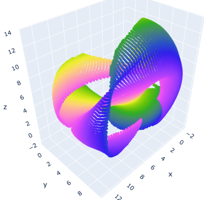
(a)

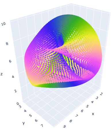
(b)

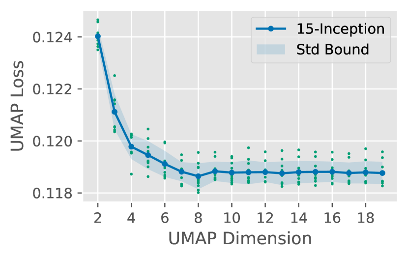
(c)

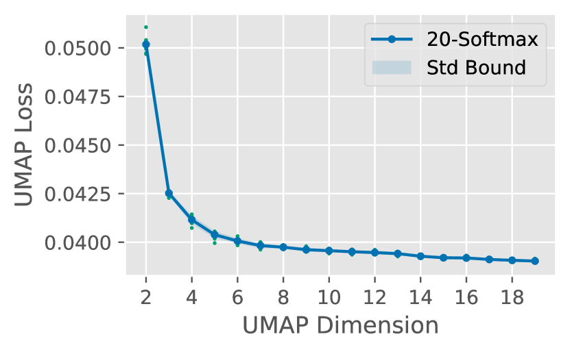
(d)

Figure 1: (a) Embedding a Klein bottle in 3D. The surface is tore apart due to UMAP’s repulsive force. (b) Embed Klein bottle in 4D and visualize in 3D. The surface is displayed continuously but has self-intersections. (c) and (d) Embedding neuron activation to more dimensions continuously improves the UMAP embedding loss. (c) In the 15-Inception layer ($40768$-D), the loss decreases until 8 dimensions and stabilized afterward. (d) In 20-Softmax ($1000$-D), loss continues to improve till the largest dimension we considered.

On realistic data, multi-dimensional UMAP also demonstrates its strength in preserving data structures. As we have described, UMAP works by preserving the neighbor graph. UMAP achieves this by finding an embedding that minimizes the binary cross entropy loss between the true neighborhood graph in the data space and the induced neighborhood graph in the embedding. Having more dimensions in the embedding space naturally gives UMAP more room to optimize the layout and therefore yields a lower loss. Here we evaluate the impact of embedding dimensions on neuron activation data. In Figure 1(c) and 1(d), we plot the loss of UMAP as we vary the embedding dimensions. When applying UMAP on the activation of 15-Inception layer of a well-trained GoogLeNet model (Figure 1(c)), we see a large gain from 2D to 4D, followed by smaller improvement from 4D to 8D, and a plateau afterward. On the final softmax layer (Figure 1(d)), we see the loss continues to improve until as far as 19 dimensions. In the supplementary material we report the same analysis on other layers of GoogLeNet. This empirical analysis of UMAP dimensionality suggests a potential benefit of embedding data to more than 3 dimensions. In theory, one should embed data into a space with dimensionality no less than the intrinsic dimensionality of the data manifold, as $n$-manifolds can not be homeomorphically embedded in less than $n$ dimensions. In practice, however, it is not straightforward to estimate the intrinsic dimensionality of data manifolds and choose the optimal embedding dimension accordingly. Throughout the experiments and visualizations in this work, we empirically use $15$ dimensional UMAP to maintain the structure in the embedding while ensuring a good real-time performance of the visualization.

2.2 Neural Network Visualizations

People have been visualizing neural networks via different angles, including saliency maps Selvaraju et al. (2017); Zeiler & Fergus (2014); Bach et al. (2015); Ancona et al. (2019), feature visualizations Olah et al. (2017), embedding methods Karpathy (2012); Rauber et al. (2016); Li et al. (2020), loss landscapesLi et al. (2018) or combinations of methods Olah et al. (2018); Carter et al. (2019). While most embedding-based visualizations project the high-dimensional data into 2 or 3 dimensions, Li et al. Li et al. (2020) linearly project the internal representation onto more than 3 dimensions (using PCA) and used the Grand Tour to visualize the neuron activations in small neural networks. We take a similar visual approach to Li et al., but extend their method in scalability and generality. Instead of linearly project neuron activations, we non-linearly project them via UMAP. Our method is more flexible and suitable for larger and real-world models. Besides, Li et al. were only able to align consecutive layers using the singular value decomposition (SVD) of fully connected layers. Our method aligns any pair of layers (Section 2.3.2). Our method works even when the two layers come from different neural network architectures. Due to this, our method can be used to compare neural architectures (Section 4).

2.2.1 The Grand Tour

The Grand Tour Asimov (1985) is a general method to visualize high dimensional data. It works by rotating the multi-dimensional data points and projecting it to 2D for display. It is a multi-dimensional analogy to ‘filming a spinning 3D object and display it on a 2D screen’. People make sense of high dimensional data through this animated 2D scatter plot rendered by a smooth sequence of 2D projections. Formally, the Grand Tour designs a smooth sequence of orthogonal matrices $GT_{t}\in\mathbb{R}^{p\times p}$ (e.g. using torus method Asimov (1985)) which is parametrized by time step $t$. It then uses this sequence to project p-dimensional data points $X\in\mathbb{R}^{n\times p}$ and we visualize the first $2$ components of the projection. In other words, we visualize smoothly animated data points $\{(x_{i}(t),y_{i}(t)),i=1\dots n\}$ in a 2D scatter plot, where each data point $X_{i}\in\mathbb{R}^{1\times p}$ is handled by the Grand Tour rotation $GT_{t}$ followed by an orthogonal projection $P_{2}:(x_{1},x_{2},\dots,x_{p})\mapsto(x_{1},x_{2})$ onto the xy-plane:

$$(x_{i}(t),y_{i}(t))=X_{i}\cdot GT_{t}\cdot P_{2}$$ (1)

Several extensions of the Grand Tour provides controls and constraints to the projection Cook et al. (1995); Cook & Buja (1997); Cook et al. (2008). Cook et al. Cook & Buja (1997) provides manual controls through tuning the contribution of each variable. Instead of controlling the contribution of variables in the projection Cook & Buja (1997), we take the more intuitive approach proposed by Li et al. (2020). As a result, our interface allows the viewer to directly drag a subset of data points to any desired location.

2.3 Similarity Measures and Alignments

Previous studies have proposed different notions of similarities between neural network representations Raghu et al. (2017); Morcos et al. (2018); Kornblith et al. (2019). Kornblith et al. Kornblith et al. (2019) observed that centered kernel alignment (CKA) has three desirable invariance properties: invariance with respect to rotations, isotropic scaling while being not invariant to general invertible linear transforms. In Table 1, we compare CKA, our proposal, and other methods.

Table 1: Comparing similarity indices. Our method satisfies all three invariants of CKA Kornblith et al. (2019). Other methods, such as linear regression, SVCCA Raghu et al. (2017) and PWCCA Morcos et al. (2018) fail to satisfy some of these properties. In addition, our method provides a scalable, instance-level and well-aligned visualization.

	Non-invariant to	Invariant to			Instance-level Visualization
	Linear Transform	Orthogonal Transform	Isotropic Scaling	Scalable		Alignment
Others	✓/✗/conditional	✓/✗	✓/✗	?	?	?
CKA	✓	✓	✓	✗	✗	?
UMAP + Procrustes (Ours)	✓	✓	✓	✓	✓	✓

2.3.1 Centered Kernel Alignment

A key insight from CKA is that instead of comparing multivariate features of examples, we can compare the structure of two representations through pairwise similarities between input instances. Although CKA works for any kernels, for simplicity, we only consider similarity using linear kernels (i.e. dot product). Given two layer representations $X$ and $Y$, the pairwise similarities among examples are encoded in the Gram matrices $K=XX^{T}$ and $L=YY^{T}$. One can measure the similarity between these two structures by their dot product: $\langle K,L\rangle=\sum_{i,j=1}^{n}K_{ij}L_{ij}=tr(XX^{T}YY^{T})=||X^{T}Y||_{F}^{2}$. Once $X$ and $Y$ are centralized, denoted by $\hat{X}$ and $\hat{Y}$, the dot product resembles the squared Frobenius norm of cross-covariance matrix between $X$ and $Y$: $\langle\hat{K},\hat{L}\rangle=||\hat{X}^{T}\hat{Y}||_{F}^{2}=||cov(X^{T},Y^{T})||_{F}^{2}$. CKA normalizes this dot product to make it invariant to isotropic scaling:

$$CKA_{Linear}(X,Y)=\frac{||\hat{X}^{T}\hat{Y}||_{F}^{2}}{||\hat{X}^{T}\hat{X}||_{F}||\hat{Y}^{T}\hat{Y}||_{F}}$$ (2)

In the next session we will show that with a simple change of the norm, we can design another similarity measure which satisfy all three invariances while having a simpler geometric interpretation.

2.3.2 Orthogonal Procrustes Problems

As we have explained, the Grand Tour smoothly rotates data using a sequence of orthogonal transformations. In other words, the visualization is invariant to rotations. Trying to align two rotationally invariant visualizations naturally gives us an orthogonal Procrustes problem Gower et al. (2004). The alignment also induces a new similarity index, similar to CKA, that is invariant to rotation but not invariant to other invertible linear transformations.

We first define orthogonal Procrustes problems. Given two representations $X\in\mathbb{R}^{n\times p_{1}}$ and $Y\in\mathbb{R}^{n\times p_{2}}$, we further assume $p_{1}=p_{2}=p$. Orthogonal Procrustes problem looks for an orthogonal transformation $Q\in\mathbb{R}^{p\times p}$ that minimizes the squared euclidean distance between $Y$ and the transformed $X$:

$$argmin_{Q}\;||XQ-Y||_{F}^{2}\text{,\quad subject to }Q^{T}Q=I$$

Geometrically, orthogonal Procrustes problem looks for the best rotation $Q$ that aligns $X$ with respect to $Y$, without scaling $X$. The optimum is achieved when $Q^{*}=UV^{T}$, where $U$ and $V$ are the singular matrices of $X^{T}Y$, i.e. $U\Sigma V^{T}=X^{T}Y$. See Gower et al. (2004) for the derivation.

Connection to CKA To see how orthogonal Procrustes relates to CKA, we follow the notes in Kornblith et al. (2019). The squared Frobenius norm in the minimization can be expanded into $||XQ-Y||_{F}^{2}=||X||_{F}^{2}+||Y||_{F}^{2}-2tr(Y^{T}XQ)$. The two norms are constants, therefore minimizing $||XQ-Y||_{F}^{2}$ is equivalent to maximizing the trace $tr(Y^{T}XQ)$. Plugging the optimum $Q^{*}=UV^{T}$ into the maximization shows that the maximum evaluates to $max_{Q}\;tr(Y^{T}XQ)=tr(\Sigma)=||X^{T}Y||_{*}$, where $||\cdot||_{*}$ denotes the nuclear norm, i.e. the sum of singular values of $X^{T}Y$. Note this resembles the numerator of linear CKA in Eq  2, with the squared Frobenius norm replaced by a nuclear norm. With this connection in mind, we can define a new similarity measure based on orthogonal Procrustes.

$$s_{op}(X,Y)=\frac{||X^{T}Y||_{*}}{\sqrt{||X^{T}X||_{*}||Y^{T}Y||_{*}}}$$ (3)

This is in the same form as Eq. 2, where every squared Frobenius norm is replaced by a nuclear norm. This similarity index satisfies all the three desired invariances that CKA possessed. In addition, this similarity index has a straightforward geometric interpretation: it measures the degree of alignment of two configurations when rotating one of them toward the other. More importantly, the alignment associated with this similarity can be used to match instance-level visualizations of different layer representations. Here we emphasize the importance of alignment because a single number for comparing two layers is not enough. To see why, note that similarity index depends on the choice of probing input examples. Probing with different examples can yield different pictures of layer-wise similarities. Figure 2.3.2 illustrates this phenomenon: when probing the layers with pictures from difference classes, the CKA reports different scores between layers. Therefore, an instance-level visualization and easy-to-interpret alignment is needed to understand the layer behavior than a list of numbers. Table 1 summarizes the strength of our method over CKA and other aligning methods discussed in Kornblith et al. (2019). In UMAP Tour, we use orthogonal Procrustes to align two dimensionality reduced representations.

Figure 2(()): CKA of GoogLeNet layers given by instances from different classes. Top: CKA from examples from 4 individual classes. Bottom: Deviation of each class from the mean CKA of 1000 classes.

Figure 2(()): Comparing linear CKA with orthogonal Procrustes. Orthogonal procrustes produces similar scores and block structures to linear CKA.

 

2.3.3 Alignment between Embeddings

The UMAP embeddings on two different layers are learned independently and therefore not aligned by default. To better compare two embeddings, we use orthogonal Procrustes to align the two embedded representations. We align the UMAP embeddings instead of the neuron activation vectors, to scale our method to real-world models. Orthogonal Procrustes relies on singular value decomposition of $X^{T}Y\in\mathbb{R}^{p\times p}$, whose runtime complexity is cubic to the number of features ($p$) in data Golub & Van Loan (2013). UMAP greatly reduces the dimensionality and makes the alignment much faster in practice. As importantly, UMAP is able to capture most of structures in data with manageable loss of preciseness. In Figure 2.3.2, we compare the layer-level similarities measured by CKA on the original neuron activations with the ones measured by orthogonal Procrustes on the 15 dimensional UMAP embeddings. We trained 4 all-convolutional nets Springenberg et al. (2014) with different depths on the CIFAR-10 dataset Krizhevsky et al. (2009), following the configuration in Kornblith et al. (2019). Even though UMAP greatly reduced the dimensionality of data, we see the two mechanisms returns similar scores and similar block structures in the similarity matrices. The Pearson’s r between two metrics for these four examples are 0.9493, 0.9384, 0.8953 and 0.9618 respectively, showing a consistently good linear relation between these two metrics.

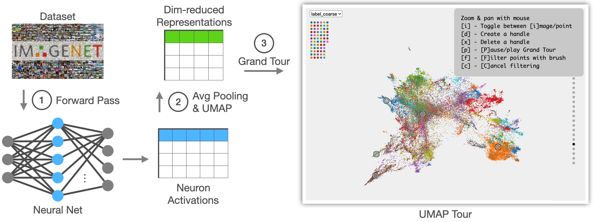
Figure 3: The UMAP Tour pipeline and the user interface.

3 Method

The basic steps of UMAP Tour is straightforward: we first take a dataset and pass it to the neural network of interest and record the neuron activations in every layer. Next, for each layer we use UMAP to project the activation to a few (e.g. $15$) dimensions. Finally, we use the Grand Tour to visualize the embeddings. The three steps are summarized in Figure 3. When moving from layer to layer or comparing two models side by side, we use procrustes transforms to align the views of instance-level representations (see Section 3.2.2).

3.1 Data Preprocessing

We start by choosing both a neural network and dataset of interest. The dataset serves as a probe of the internal behavior of the neural network. It does not have to be the training or validation set on which the model was trained or validated. For example, even though GoogLeNet Szegedy et al. (2015) is most commonly trained on ImageNet Deng et al. (2009), we can either use ImageNet or other image datasets to validate concepts learned by GoogLeNet. In Section 4, we use a pre-trained GoogLeNet and probe it with the validation set of ImageNet Deng et al. (2009). In the supplementary material we include experiments with an out-of-training face dataset Kärkkäinen & Joo (2019). Although we are aware of the ethical issues with ImageNet, and share the concerns over its nonconsensual content Prabhu & Birhane (2020), a direct comparison to existing results in the literature requires us to use the dataset.

As the first step, we pass image examples to the network and store the neuron activations of each layer. The number of neurons in a layer can be very large, usually in the order of hundreds of thousand dimensions for convolutional layers, which makes it hard to visualize in practice. In the second step, we use UMAP to reduce the number of features to a manageable size. We project neuron activations to $15$ dimensions in order to capture enough interesting structures in the data. When fitting the UMAP embeddings, we keep all hyperparameters as default except for the embedding dimensions.  We chose UMAP for its good runtime performance, flexibility and reliability to capture global structures in the data, although method works for other dimensionality reduction techniques. In this specific case, however, UMAP alone is still not practical for handling $\sim 100$k dimensional neuron activation data. Even though UMAP scales reasonably well with the number of dimensions, it is still time consuming to apply UMAP directly on activations with, for example, all spatial dimensions on convolutional layers with hundreds of thousand dimensions when flattened. To reduce the runtime of UMAP while preserving most of structural features in data, we apply average pooling before applying UMAP - we first use 2D average pooling to reduce the dimension (from hundreds of thousand) to a few tens of thousand, and then apply UMAP on the average-pooled activations. See supplementary for more on the computing infrastructure used, exact dimension and runtime of each layer.

3.2 Visualization

As the final step, we use the Grand Tour Asimov (1985) to visualize ‘every aspect’ of the embedding space using an animated scatter plot. At the end of the pipeline (Figure 3) we show our user interface. We used WebGL and D3.js Bostock et al. (2011) to build a scalable web interface. As an example, Figure 3 shows $50k$ images from ImageNet. In the central Grand Tour view, user can zoom and pan via mouse sweep. In addition, user can steer the projection by directly selecting and dragging Li et al. (2020) data points. On top left of the interface (Figure 3), user can color data points by attributes via the option menu, such as coloring by label, prediction confidence or prediction error. The color legend below will change accordingly. On the right, user can switch to different layers of the model by clicking on the gray dots. The transitions between layers are made smooth via orthogonal Procrustes. To compare two models, we take two Grand Tour views, align and display them side by side (Figure 7, left). We also draw the layer-wise similarities as a heatmap on the bottom. Clicking on any entry of the similarity matrix quickly switches to the corresponding pair of layers. Other functionalities, such as direct manipulation, can be enabled via keyboard shortcuts as explained in the top right pop-up. For example, user can switch to original images by pressing [i], manipulate projections by [d] or apply spatial filters by [f].

3.2.1 Direct Manipulation

The Grand Tour, by default, walks through all possible projections in a predetermined, but somewhat random manner. Controlling the projection would let users navigate to the views of their own interest, instead of waiting for them to come. Manual control should imply changes on the entries of the Grand Tour projection matrix $GT\in\mathbb{R}^{p\times p}$. Specifically, since data points are projected via Eq.1, the first two components in every $j^{th}$ row of the $GT$ determines where each standard basis vector $e_{j}$ is projected in the plot. Before Li et al. (2020), the control is typically done via a separate interface where user selects one of the $p$ variables and change its contribution in x or y direction. However, controlling each variable is not as intuitive as moving data points. This is especially true for embeddings, as each variable in the UMAP embedding may not come with semantics. See Li et al. (2020) for details.

3.2.2 Aligning representations

Transition between layers: When visualizing one model with UMAP Tour, we switch the view between layers through a smooth and traceable transition. Specifically, when switching from one layer $Y$ to another $X$, we first align the next layer $X$ against the previous layer $Y$ via orthogonal Procrustes $Q^{*}$. Next, we linearly interpolate the two aligned representations $Y$ and $XQ^{*}$: $X(s)=(1-s)\cdot Y+s\cdot XQ^{*}$. Finally, the interpolation is viewed via Grand Tour projection as in Eq.1.

Aligning architectures: When visualizing two models side by side, we align their layer representations in the same manner using orthogonal Procrustes. When comparing the UMAP embedding of one model $Y$ with the embedding $X$ from another model, we show $Y$ and $XQ^{*}$ side by side in UMAP Tour. When directly manipulation is applied on any one of the views, the change is applied to both views so that the views are kept aligned (Figure 7).

4 Use Cases

We test our method for visualizing a single neural network and comparing two neural networks. Using GoogLeNet as an example, we first visualize its training process. This was referred to as training dynamics by Li et al. Li et al. (2018). Following their terminology, we explain the layer dynamics of GoogLeNet - how examples flow through the layers. We found unexpected concepts learned in GoogLeNet layers, such as human faces. Finally, we compare two different neural architectures. We found that they demonstrate instance-level difference while preserving some layer-level similarity.

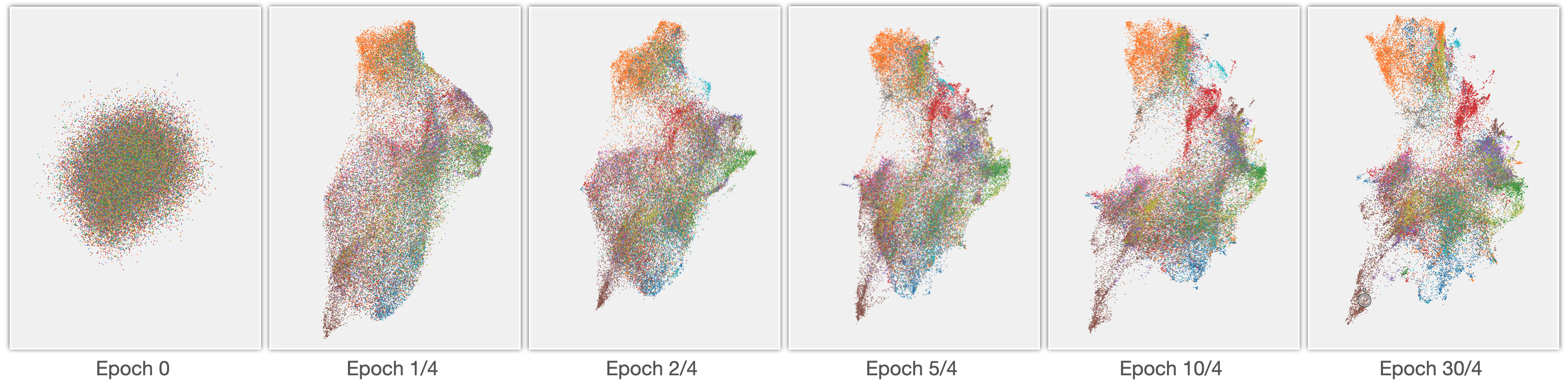
Figure 4: Training dynamics of GoogLeNet on 16-Inception layer.

4.1 Training Dynamics

We first trained a GoogLeNet from scratch with standard data augmentation strategies on the training set of ImageNet Deng et al. (2009). We optimize the cross-entropy loss (on both the main and auxiliary classifiers) with an Adam Kingma & Ba (2014) optimizer using mini-batches of size 64. We save the state of the model once its initialized as well as on every $1/4$ epoch ($\approx 0.32M$ examples the training set). Figure 4 illustrates how UMAP Tour interprets a layer during this training process. Starting from a single blob, the examples are gradually split into class-related regions throughout the training. Notice how dog images (orange dots on top) are first gathered on top and later spitted into smaller clusters.

4.2 Layer Dynamics

Recent works Olah et al. (2017); Cammarata et al. (2020); Goh et al. (2021); Hohman et al. (2019) have found explanations to how neural networks learn high-level concepts from low-level features. UMAP Tour sheds some light onto this via a different angle. Since an image classifier is a mapping from raw pixel colors to the label of the object, one should expect very early layers capture low-level features such as overall color and final layers summarize features into high-level concepts such as object classes. UMAP Tour is able to show this layer dynamics and reveals how a sequence of intermediate layers approach certain goal in multiple steps.

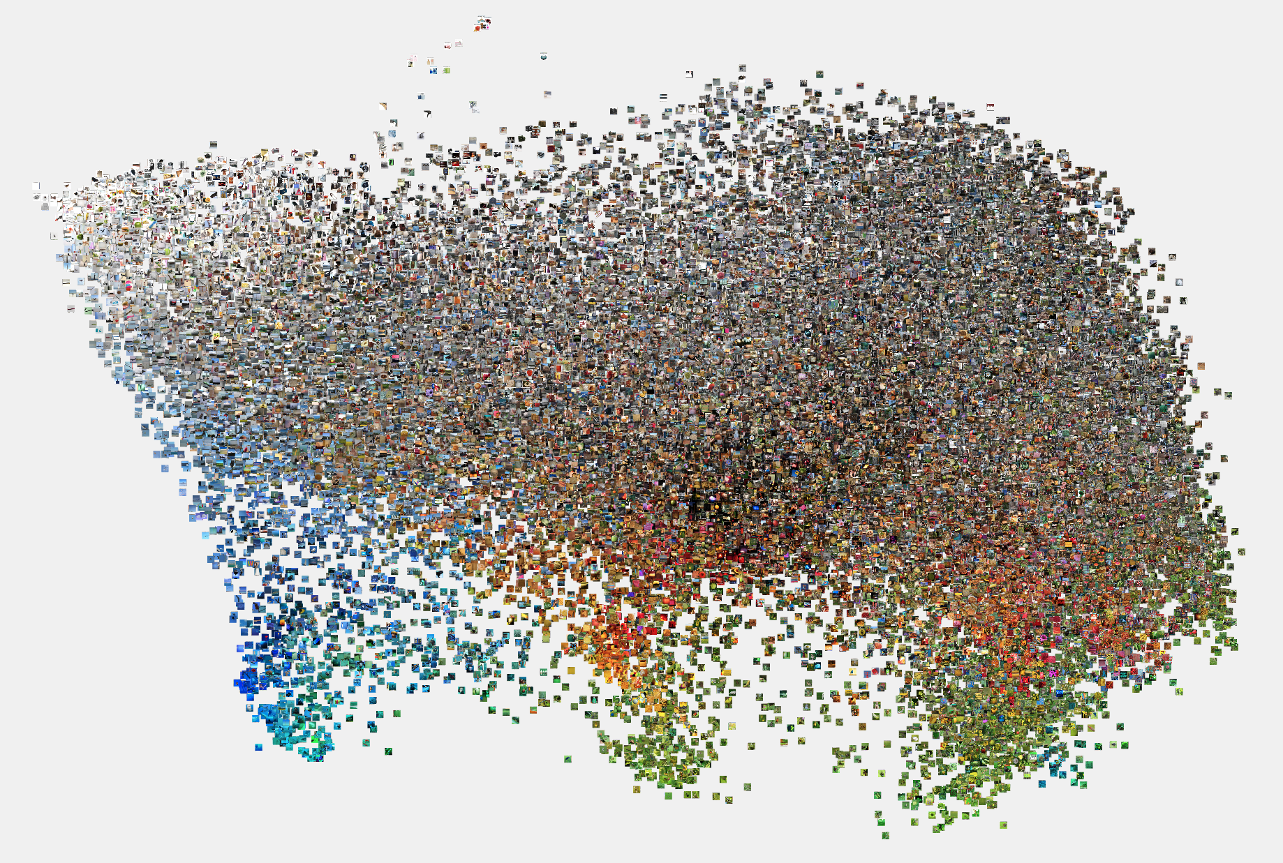
Figure 5(()): Images arranged by colors in the 1-BasicConv2D layer.

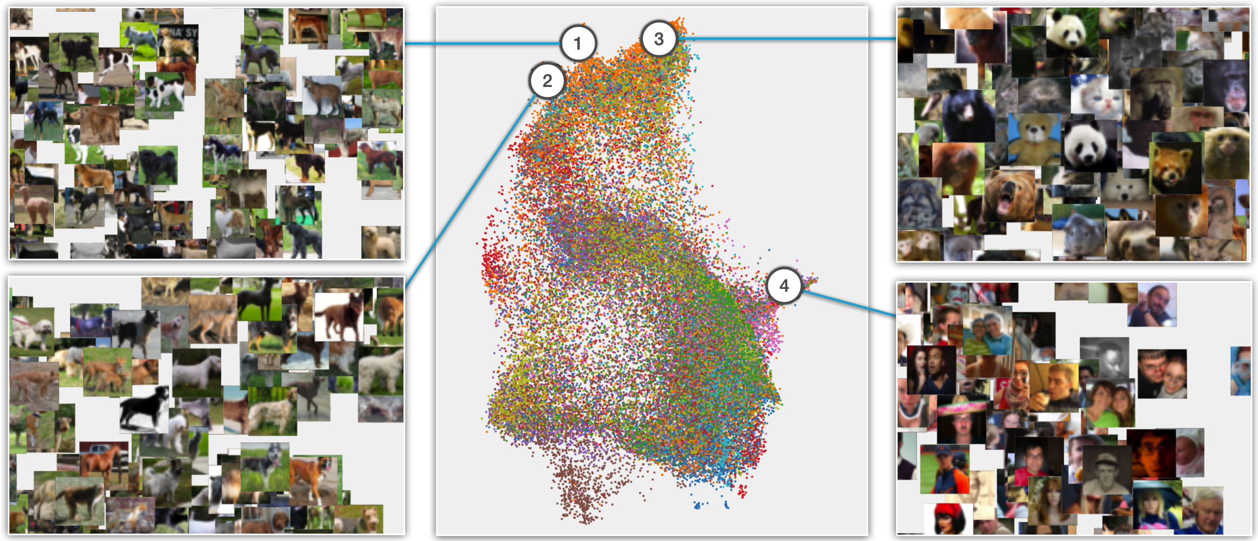
Figure 5(()): Concepts learned in the 12-Inception layer: ➀➁ Orientation of dogs; ➂ animal faces; and ➃ human faces.

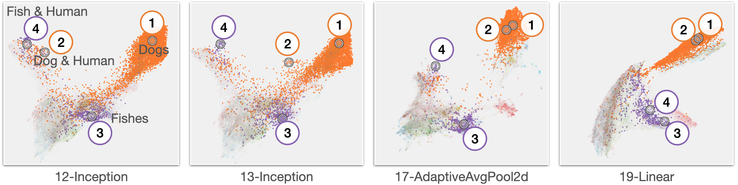
Figure 6: Layer dynamics in GoogLeNet. GoogLeNet considers existence of humans as a factor when classifying other objects. From the 12-Inception layer to 17-AdaptiveAvgPool2d, dog-with-human images (➁) moves from the a cluster of humans to the cluster of $\bullet$ dogs (➀), while the fish-with-human images (➃) remain stable in the view. The fish-with-human (➃) moves closer to the other $\bullet$ fishes (➂) only after the penultimate (19-Linear) layer.

At early layers, images arranged primarily by color, as shown in Figure 4.2. Later, the model encodes orientation of animals (e.g. dogs and birds) despite being only trained to classify them (Figure 4.2). In the same layer, the network also recognizes human faces, despite few human label is provided during training. When classifying objects that may or may not appear with human (e.g. dogs alone or with their owners, fishes in the wild or held by humans), GoogLeNet considers the two cases separately (Figure 6). Diving down from 12-Inception layer to a deeper global pooling layer (17-AdaptiveAvgPool2D), we observed a small group of dog-with-human images gradually moves toward the main cluster of dogs. On the other hand, the cluster of images showing fish caught by human remains stable. They only move to the cluster of fishes in the penultimate fully connected layer (19-Linear). This demonstrates the layer dynamics of model in UMAP Tour. The revealed patterns in each layer can be particularly useful in, for instance, finding the best layer for transfer learning.

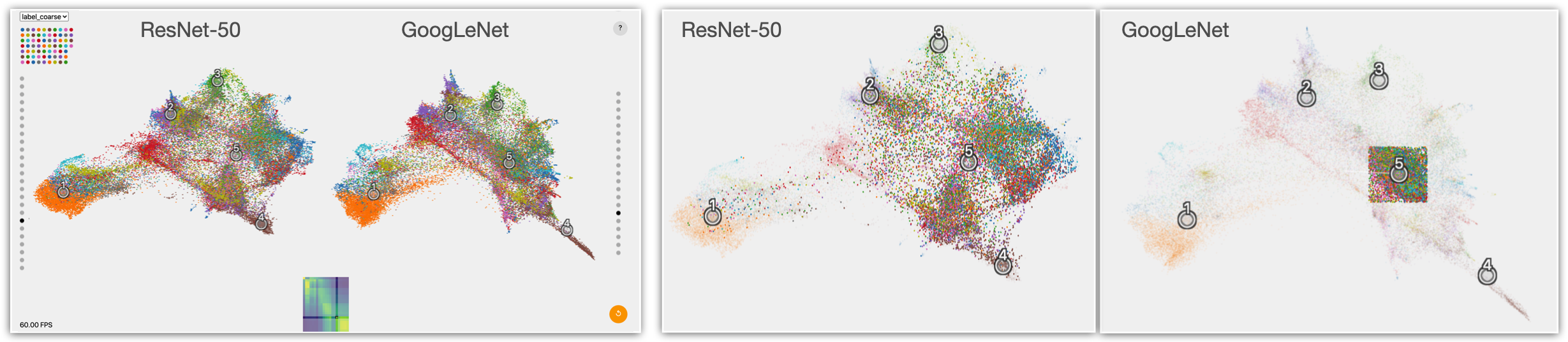
Figure 7: Comparing ResNet-50 (18-Bottleneck layer) with GoogLeNet (15-Inception layer). The two layers give a similarity score of 0.810. Left: UI. Right: The two views match in many landmarks, such as ➀ dogs, ➁ bugs and snakes, ➂ food and ➃ vehicles. However, filtering around ➄ reveals GoogLeNet’s unique cluster of (electronics, buildings and clothings) not formed in ResNet-50.

4.3 Comparing Two Models

Although many works has been done to visually interpret the internal of neural networks Olah et al. (2017); Nguyen et al. (2019); Selvaraju et al. (2017), fewer of them is able to directly compare two architectures. UMAP Tour is designed for comparison especially when equipped with orthogonal Procrustes. For example, ResNet-50 and GoogLeNet have a similar index $0.810$ on a pair of intermediate layers. In UMAP Tour, we see similar and well-aligned UMAP embeddings in these layers, as shown by some landmarks (➀-➃ in Figure 7). In addition to the similarity, UMAP Tour also shows the dissimilarity between the two: GoogLeNet as a unique cluster of man-made objects (electronics, buildings, clothings, etc) which is more distributed in ResNet-50 (➄ in Figure 7). In other words, UMAP Tour not only uses the similarity as a measure to align two representations, but also explains their dissimilarities in its instance-level visualizations.

5 Discussion

Orthogonal Procrustes or CKA? It depends. The CKA can be easy to compute, since the Frobenius norm only requires summation over the square of the entries. The similarity derived from orthogonal Procrustes, in contrast, requires finding or estimating nuclear norms. To our knowledge, this is still under active research Heavner & Martinsson (2019). In UMAP Tour, we reduce runtime by reducing data dimensionality with UMAP and believe the resultant alignment from orthogonal Procrustes is more valuable than the similarity score. Aligning instance-level details with orthogonal Procrustes is interpretable and intuitive - it simply rotates one configuration to another, without any scaling. Meanwhile, although the similarity index of CKA is not invariant to general linear transform, we found its alignment does contain scaling factors along the singular directions. See Appendix for details.

Non-linear or linear dimensionality reduction? Although Li et al. Li et al. (2020) have advocated and demonstrated the theoretical benefits of using linear methods (i.e. PCA and the Grand Tour), we believe non-linear methods such as UMAP has its stance in practice. To explain a large model with millions of dimensions in one layer, PCA may require a large number of dimensions to have a good coverage of variance. On the other hand, rendering the Grand Tour in real time with high frame rate (e.g. 60 fps) using WebGL puts a limit to the number of dimensions we can render (e.g. by the maximum number of vertex attributes allowed in GLSL). To handle this trade-off, linear methods (e.g. PCA) usually put a hard stop at certain dimension while non-linear methods handle this in a more flexible way. Within a limited budget of embedding dimensions, non-linear methods seem to summarize data relations of high dimension spaces more easily. See Appendix for details.

Orthogonal Procrustes or SVD? Comparing to the SVD method used by Li et al. Li et al. (2020), orthogonal Procrustes generates a slightly different alignment between linearly connected layers and works beyond linear cases. Recall that when two layers are related by a linear transformation $Y=XW$, Li et al. align two layers by the SVD of $W$ - i.e. they align layers by $U_{W}V^{T}_{W}$ where $U_{W}$ and $V_{W}$ are singular matrices of $W$. If $X$ varies uniformly along all directions (which can be the case under certain circumstances, e.g. after batch norm layers), the two methods tend to generate similar alignments, although the SVD only works for linear layers. See Appendix for details.

6 Conclusion

In this work we explored how classical visual method (the Grand Tour) can be combined with modern embeddings (namely UMAP) to reason instance-level behavior of deep neural networks. We build UMAP Tour and use it to visualize patterns within state-of-the-art models such as GoogLeNet and ResNet-50. The alignment method used in this visualization, namely orthogonal Procrustes on the UMAP embedding, naturally induces a new similarity measure between neural network layers. Empirically, we find this measure numerically comparable to CKA, while the alignment gives us an intuitive, instance-level visual comparison between layers. Our visualization built around these notions has revealed patterns in the model internals and shed some light on the transparency and fairness concerns of neural networks.

References

- Ancona et al. (2019) Ancona, M., Oztireli, C., and Gross, M. Explaining deep neural networks with a polynomial time algorithm for shapley value approximation. In International Conference on Machine Learning, pp. 272–281. PMLR, 2019.
- Asimov (1985) Asimov, D. The grand tour: a tool for viewing multidimensional data. SIAM journal on scientific and statistical computing, 6(1):128–143, 1985.
- Bach et al. (2015) Bach, S., Binder, A., Montavon, G., Klauschen, F., Müller, K.-R., and Samek, W. On pixel-wise explanations for non-linear classifier decisions by layer-wise relevance propagation. PloS one, 10(7):e0130140, 2015.
- Borg & Groenen (2005) Borg, I. and Groenen, P. J. Modern multidimensional scaling: Theory and applications. Springer Science & Business Media, 2005.
- Bostock et al. (2011) Bostock, M., Ogievetsky, V., and Heer, J. D3 data-driven documents. IEEE Transactions on Visualization and Computer Graphics, 17(12):2301–2309, December 2011. ISSN 1077-2626. doi: 10.1109/TVCG.2011.185. URL https://doi.org/10.1109/TVCG.2011.185.
- Cammarata et al. (2020) Cammarata, N., Carter, S., Goh, G., Olah, C., Petrov, M., and Schubert, L. Thread: Circuits. Distill, 5(3):e24, 2020.
- Carlsson et al. (2008) Carlsson, G., Ishkhanov, T., De Silva, V., and Zomorodian, A. On the local behavior of spaces of natural images. International journal of computer vision, 76(1):1–12, 2008.
- Carter et al. (2019) Carter, S., Armstrong, Z., Schubert, L., Johnson, I., and Olah, C. Exploring neural networks with activation atlases. Distill., 2019.
- Cook & Buja (1997) Cook, D. and Buja, A. Manual controls for high-dimensional data projections. Journal of computational and Graphical Statistics, 6(4):464–480, 1997.
- Cook et al. (1995) Cook, D., Buja, A., Cabrera, J., and Hurley, C. Grand tour and projection pursuit. Journal of Computational and Graphical Statistics, 4(3):155–172, 1995.
- Cook et al. (2008) Cook, D., Buja, A., Lee, E.-K., and Wickham, H. Grand tours, projection pursuit guided tours, and manual controls. In Handbook of data visualization, pp. 295–314. Springer, 2008.
- Deng et al. (2009) Deng, J., Dong, W., Socher, R., Li, L., Li, K., and Li, F. Imagenet: A large-scale hierarchical image database. In 2009 IEEE Computer Society Conference on Computer Vision and Pattern Recognition (CVPR 2009), 20-25 June 2009, Miami, Florida, USA, pp. 248–255. IEEE Computer Society, 2009. doi: 10.1109/CVPR.2009.5206848. URL http://www.image-net.org/.
- Goh et al. (2021) Goh, G., Cammarata, N., Voss, C., Carter, S., Petrov, M., Schubert, L., Radford, A., and Olah, C. Multimodal neurons in artificial neural networks. Distill, 6(3):e30, 2021.
- Goldfeld et al. (2018) Goldfeld, Z., Berg, E. v. d., Greenewald, K., Melnyk, I., Nguyen, N., Kingsbury, B., and Polyanskiy, Y. Estimating information flow in deep neural networks. arXiv preprint arXiv:1810.05728, 2018.
- Golub & Van Loan (2013) Golub, G. and Van Loan, C. Matrix computations 4th edition the johns hopkins university press. Baltimore, MD, 2013.
- Gower et al. (2004) Gower, J. C., Dijksterhuis, G. B., et al. Procrustes problems, volume 30. Oxford University Press on Demand, 2004.
- Heavner & Martinsson (2019) Heavner, N. and Martinsson, P.-G. Efficient nuclear norm approximation via the randomized utv algorithm. arXiv preprint arXiv:1903.11543, 2019.
- Hohman et al. (2019) Hohman, F., Park, H., Robinson, C., and Chau, D. H. P. S ummit: Scaling deep learning interpretability by visualizing activation and attribution summarizations. IEEE transactions on visualization and computer graphics, 26(1):1096–1106, 2019.
- Kärkkäinen & Joo (2019) Kärkkäinen, K. and Joo, J. Fairface: Face attribute dataset for balanced race, gender, and age. arXiv preprint arXiv:1908.04913, 2019. URL https://github.com/dchen236/FairFace.
- Karpathy (2012) Karpathy, A. t-sne visualization of cnn codes, 2012. URL https://cs.stanford.edu/people/karpathy/cnnembed/.
- Kim et al. (2018) Kim, B., Wattenberg, M., Gilmer, J., Cai, C. J., Wexler, J., Viégas, F. B., and Sayres, R. Interpretability beyond feature attribution: Quantitative testing with concept activation vectors (TCAV). In Proceedings of the 35th International Conference on Machine Learning, ICML 2018, Stockholmsmässan, Stockholm, Sweden, July 10-15, 2018, volume 80 of Proceedings of Machine Learning Research, pp. 2673–2682. PMLR, 2018.
- Kingma & Ba (2014) Kingma, D. P. and Ba, J. Adam: A method for stochastic optimization. arXiv preprint arXiv:1412.6980, 2014.
- Kornblith et al. (2019) Kornblith, S., Norouzi, M., Lee, H., and Hinton, G. E. Similarity of neural network representations revisited. In Proceedings of the 36th International Conference on Machine Learning, ICML 2019, 9-15 June 2019, Long Beach, California, USA, volume 97 of Proceedings of Machine Learning Research, pp. 3519–3529. PMLR, 2019.
- Krizhevsky et al. (2009) Krizhevsky, A., Nair, V., and Hinton, G. Cifar-10 (canadian institute for advanced research). 2009. URL http://www.cs.toronto.edu/~kriz/cifar.html.
- Lan et al. (2020) Lan, Z., Chen, M., Goodman, S., Gimpel, K., Sharma, P., and Soricut, R. ALBERT: A lite BERT for self-supervised learning of language representations. In 8th International Conference on Learning Representations, ICLR 2020, Addis Ababa, Ethiopia, April 26-30, 2020. OpenReview.net, 2020.
- Li et al. (2018) Li, H., Xu, Z., Taylor, G., Studer, C., and Goldstein, T. Visualizing the loss landscape of neural nets. In Proceedings of the 32nd International Conference on Neural Information Processing Systems, pp. 6391–6401, 2018.
- Li et al. (2020) Li, M., Zhao, Z., and Scheidegger, C. Visualizing neural networks with the grand tour. Distill, 5(3):e25, 2020.
- McInnes (2018) McInnes, L. Performance comparison of dimension reduction implementations, 2018. URL https://umap-learn.readthedocs.io/en/latest/benchmarking.html.
- McInnes et al. (2018) McInnes, L., Healy, J., and Melville, J. Umap: Uniform manifold approximation and projection for dimension reduction. arXiv preprint arXiv:1802.03426, 2018.
- Morcos et al. (2018) Morcos, A. S., Raghu, M., and Bengio, S. Insights on representational similarity in neural networks with canonical correlation. In Advances in Neural Information Processing Systems 31: Annual Conference on Neural Information Processing Systems 2018, NeurIPS 2018, December 3-8, 2018, Montréal, Canada, pp. 5732–5741, 2018.
- Nguyen et al. (2019) Nguyen, A., Yosinski, J., and Clune, J. Understanding neural networks via feature visualization: A survey. In Explainable AI: interpreting, explaining and visualizing deep learning, pp. 55–76. Springer, 2019.
- Olah et al. (2017) Olah, C., Mordvintsev, A., and Schubert, L. Feature visualization. Distill, 2(11):e7, 2017.
- Olah et al. (2018) Olah, C., Satyanarayan, A., Johnson, I., Carter, S., Schubert, L., Ye, K., and Mordvintsev, A. The building blocks of interpretability. Distill, 3(3):e10, 2018.
- Prabhu & Birhane (2020) Prabhu, V. U. and Birhane, A. Large image datasets: A pyrrhic win for computer vision? arXiv preprint arXiv:2006.16923, 2020.
- Raghu et al. (2017) Raghu, M., Gilmer, J., Yosinski, J., and Sohl-Dickstein, J. SVCCA: singular vector canonical correlation analysis for deep learning dynamics and interpretability. In Advances in Neural Information Processing Systems 30: Annual Conference on Neural Information Processing Systems 2017, December 4-9, 2017, Long Beach, CA, USA, pp. 6076–6085, 2017.
- Rauber et al. (2016) Rauber, P. E., Fadel, S. G., Falcao, A. X., and Telea, A. C. Visualizing the hidden activity of artificial neural networks. IEEE transactions on visualization and computer graphics, 23(1):101–110, 2016.
- Roweis & Saul (2000) Roweis, S. T. and Saul, L. K. Nonlinear dimensionality reduction by locally linear embedding. science, 290(5500):2323–2326, 2000.
- Selvaraju et al. (2017) Selvaraju, R. R., Cogswell, M., Das, A., Vedantam, R., Parikh, D., and Batra, D. Grad-cam: Visual explanations from deep networks via gradient-based localization. In IEEE International Conference on Computer Vision, ICCV 2017, Venice, Italy, October 22-29, 2017, pp. 618–626. IEEE Computer Society, 2017. doi: 10.1109/ICCV.2017.74.
- Springenberg et al. (2014) Springenberg, J. T., Dosovitskiy, A., Brox, T., and Riedmiller, M. Striving for simplicity: The all convolutional net. arXiv preprint arXiv:1412.6806, 2014.
- Sun et al. (2014) Sun, Y., Chen, Y., Wang, X., and Tang, X. Deep learning face representation by joint identification-verification. In Advances in Neural Information Processing Systems 27: Annual Conference on Neural Information Processing Systems 2014, December 8-13 2014, Montreal, Quebec, Canada, pp. 1988–1996, 2014.
- Szegedy et al. (2015) Szegedy, C., Liu, W., Jia, Y., Sermanet, P., Reed, S. E., Anguelov, D., Erhan, D., Vanhoucke, V., and Rabinovich, A. Going deeper with convolutions. In IEEE Conference on Computer Vision and Pattern Recognition, CVPR 2015, Boston, MA, USA, June 7-12, 2015, pp. 1–9. IEEE Computer Society, 2015. doi: 10.1109/CVPR.2015.7298594.
- Tenenbaum et al. (2000) Tenenbaum, J. B., De Silva, V., and Langford, J. C. A global geometric framework for nonlinear dimensionality reduction. science, 290(5500):2319–2323, 2000.
- Van der Maaten & Hinton (2008) Van der Maaten, L. and Hinton, G. Visualizing data using t-sne. Journal of machine learning research, 9(11), 2008.
- Wold et al. (1987) Wold, S., Esbensen, K., and Geladi, P. Principal component analysis. Chemometrics and intelligent laboratory systems, 2(1-3):37–52, 1987.
- Zeiler & Fergus (2014) Zeiler, M. D. and Fergus, R. Visualizing and understanding convolutional networks. In European conference on computer vision, pp. 818–833. Springer, 2014.