Abstract

Traditionally, Bayesian network structure learning is often carried out at a central site, in which all data is gathered. However, in practice, data may be distributed across different parties (e.g., companies, devices) who intend to collectively learn a Bayesian network, but are not willing to disclose information related to their data owing to privacy or security concerns. In this work, we present a federated learning approach to estimate the structure of Bayesian network from data that is horizontally partitioned across different parties. We develop a distributed structure learning method based on continuous optimization, using the alternating direction method of multipliers (ADMM), such that only the model parameters have to be exchanged during the optimization process. We demonstrate the flexibility of our approach by adopting it for both linear and nonlinear cases. Experimental results on synthetic and real datasets show that it achieves an improved performance over the other methods, especially when there is a relatively large number of clients and each has a limited sample size.

1 Introduction

Bayesian network structure learning (BNSL) is an important problem in machine learning and artificial intelligence (Koller and Friedman, 2009; Spirtes et al., 2001; Pearl, 2009; Peters et al., 2017), and has been widely adopted in different areas such as healthcare (Lucas et al., 2004) and Earth system science (Runge et al., 2019). Traditionally, BNSL is often carried out at a central site, in which all data is gathered. With the rapid development of technology and internet, it has become increasingly easy to collect data. Therefore, in practice, data is usually owned by and distributed across a number of parties, which range from mobile devices and individuals to companies and hospitals.

In many cases, these parties, which are referred to as clients, may not have a sufficient number of samples to learn a meaningful Bayesian network (BN) on their own. They may intend to collectively obtain aggregated knowledge about the BN structure, but are not willing to disclose information related to their data owing to privacy or security concerns. Consider an example in which a number of hospitals wish to collaborate in learning a BN to discover the conditional independence structure underlying their variables of interests, e.g., medical conditions. Clearly, they are not allowed to share their patients’ records because of privacy regulations. Therefore, the sensitivity nature of the data has made it infeasible to gather the data from different clients to a central site for BNSL.

Several approaches have been developed to learn BN structures in a distributed fashion. A natural approach is that each client estimates its BN structure independently using its local dataset, and share it to a central server, which applies some heuristics, e.g., voting (Na and Yang, 2010), to aggregate these estimated structures. However, this approach may lead to suboptimal performance as the information exchange among clients is rather limited, and the estimated BNs by the individual clients may not be accurate. It remains a challenge to develop an approach that integrates the local information from different clients for learning a global BN structure while not exposing the clients’ local datasets.

A principled federated learning strategy is then needed. In the past few years, federated learning has received attention in which many clients collectively train a machine learning model based on a certain coordination strategy. Each client does not have to exchange its raw data; instead, they disclose only the minimal information necessary for the specific learning task, e.g., model parameters and gradient updates, which have been shown to work well in many tasks, e.g., image classification (McMahan et al., 2017) and recommender system (Chai et al., 2020). We refer the reader to (Yang et al., 2019; Li et al., 2020; Kairouz et al., 2021) for further details and a review on federated learning.

Most of the recent federated learning approaches, e.g., federated averaging (McMahan et al., 2017), are based on continuous optimization, which may not straightforwardly apply to standard score-based BNSL methods that rely on discrete optimization, e.g., dynamic programming (Singh and Moore, 2005), greedy search (Chickering, 2002), and integer programming (Cussens, 2011). On the other hand, continuous optimization methods for BNSL have been recently developed (Zheng et al., 2018, 2020) by utilizing an algebraic characterization of acyclicity, which provides an opportunity to render federated learning possible for BNSL.

Contributions.    In this work, we present a federated learning approach to estimate the structure of BN from data that is horizontally partitioned across different parties. Our contributions are as follows:

• We propose a distributed BNSL method based on continuous optimization, using the alternating direction method of multipliers (ADMM), such that only the model parameters have to be exchanged during the optimization process.

• We demonstrate the flexibility of our approach by adopting it for both linear and nonlinear cases.

• We conduct experiments to validate the effectiveness of our approach on synthetic and real datasets.

Organization of the paper.    We describe the related work in Section 2, and the problem formulation in Section 3. In Section 4, we describe a simple privacy-preserving approach to learn linear Gaussian BNs and its possible drawbacks. We then present the proposed federated BNSL approach in Section 5. We provide empirical results to validate our approach in Section 6, and a discussion in Section 7.

2 Related Work

We provide a review on various aspects of BNSL that are relevant to our problem formulation and approach.

2.1 BNSL with Continuous Optimization

Recently, Zheng et al. (2018) developed a continuous optimization method to estimate the structure of linear BNs subject to an equality acyclicity constraint. This method has been extended to handle nonlinear models (Kalainathan et al., 2018; Yu et al., 2019; Ng et al., 2019, 2022b; Lachapelle et al., 2020; Zheng et al., 2020), interventional data (Brouillard et al., 2020), confounders (Bhattacharya et al., 2020), and time series (Pamfil et al., 2020). Using likelihood-based objective, Ng et al. (2020) formulated the problem as an unconstrained optimization problem involving only soft constraints, while Yu et al. (2021) developed an equivalent representation of directed acyclic graphs (DAGs) that allows continuous optimization in the DAG space without the need of an equality constraint. In this work, we adopt the methods proposed by Zheng et al. (2018, 2020) due to its popularity, although it is also possible to incorporate the other methods.

2.2 BNSL from Overlapping Variables

Another line of work aims to estimate the structures over the integrated set of variables from several datasets, each of which contains only samples for a subset of variables. Danks et al. (2008) proposed a method that first independently estimates a partial ancestral graph (PAG) from each individual dataset, and then finds the PAGs over the complete set of variables which share the same d-connection and d-separation relations with the estimated individual PAGs. Triantafillou and Tsamardinos (2015); Tillman and Eberhardt (2014); Triantafillou et al. (2010) adopted a similar procedure, except that they convert the constraints to SAT solvers to improve scalability. The estimated graphs by these methods are not unique and often have a large indeterminacy. To avoid such indeterminacy, Huang et al. (2020) developed a method based on the linear non-Gaussian model (Shimizu et al., 2006), which is able to uniquely identify the DAG structure. These methods mostly consider non-identical variable sets, whereas in this work, we consider the setup in which the clients have a set of identical variables, and hope to collective learn the BN structure in a privacy preserving way.

2.3 Privacy-Preserving & Distributed BNSL

To learn BN structures from horizontally partitioned data, Gou et al. (2007) adopted a two-step procedure that first estimates the BN structures independently using each client’s local dataset, and then applies further conditional independence test. Instead of using statistical test in the second step, Na and Yang (2010) used a voting scheme to pick those edges identified by more than half of the clients. These methods leverage only the final graphs independently estimated from each local dataset, which may lead to suboptimal performance as the information exchange may be rather limited. Furthermore, Samet and Miri (2009) developed a privacy-preserving method based on secure multiparty computation, but is limited to the discrete case.

For vertically partitioned data, Wright and Yang (2004); Yang and Wright (2006) constructed an approximation to the score function in the discrete case and adopted secure multiparty computation. Chen et al. (2003) developed a four-step procedure that involves transmitting a subset of samples from each client to a central site, which may lead to privacy concern.

3 Problem Formulation

Let $G=(V,E)$ be a DAG that represents the structure of a BN defined over the random vector $X=(X_{1},\dots,X_{d})$ with a probability distribution $P(X)$. The vertex set $V$ corresponds to the set of random variables $\{X_{1},\dots,X_{d}\}$ and the edge set $E$ represents the directed edges in the DAG $G$. The distribution $P(X)$ satisfies the Markov assumption w.r.t. the DAG $G$. In this paper, we focus on the linear BN given by $X=B^{\mathsf{T}}X+N$, where $B$ is a weighted adjacency matrix whose nonzero coefficients correspond to the directed edges in $G$, and $N$ is a random noise vector whose entries are mutually independent. We use the term linear Gaussian BN to refer to the linear BN in which the entries of the noise vector $N$ are Gaussian.

We consider the setting with a fixed set of $K$ clients in total, each of which owns its local dataset. The $k$-th client holds $n_{k}$ i.i.d. samples from the distribution $P(X)$, denoted as $\mathbf{x}_{k}=\{x_{k,i}\}_{i=1}^{n_{k}}$. Let $n=\sum_{k=1}^{K}n_{k}$ be the total sample size given by the sum of the sub-sample sizes $n_{k},k=1,\dots,K$. We assume here that the data from different clients follows the same distribution, and leave the non-i.i.d. setting, which may have much potential, for future investigation. Given the collection of datasets $\mathbf{x}=\bigcup_{k=1}^{K}\mathbf{x}_{k}$ from different clients, the goal is to recover the true DAG $G$ in a privacy-preserving way. We focus on the setup in which the clients have incentives to collaborate in learning the BN structure, but are only willing to disclose minimal information (e.g., model parameters and estimated DAGs) related to their local datasets. The entire dataset $\mathbf{x}$ is said to be horizontally partitioned across different clients, which implies that each local dataset shares the same set of variables but varies in samples. We also assume the existence of a central server that coordinates the learning process and adheres to the protocol.

4 Computing Sufficient Statistics with Secure Computation

Apart from the methods reviewed in Section 2.3, in this section we describe a simple approach based on secure computation to learn the structure of linear Gaussian BNs, and discuss its possible drawbacks.

Sufficient statistics.    Denote the empirical mean and covariance of $\mathbf{x}$ by $\mu_{\mathbf{x}}=(1/n)\sum_{k=1}^{K}\sum_{i=1}^{n_{k}}x_{k,i}$ and $\Sigma_{\mathbf{x}}=(1/n)\sum_{k=1}^{K}\sum_{i=1}^{n_{k}}x_{k,i}x_{k,i}^{\mathsf{T}}-\mu_{\mathbf{x}}\mu_{\mathbf{x}}^{\mathsf{T}}$, respectively. First notice that the empirical covariance matrix $\Sigma_{\mathbf{x}}$ and the total sample size $n$ are sufficient statistics for learning linear Gaussian BNs via constraint-based and score-based methods, formally stated as follows.

Remark 1.

Suppose that the ground truth DAG $G$ and the distribution $P(X)$ form a linear Gaussian BN. Given $n$ samples $\mathbf{x}$ from the distribution $P(X)$, the empirical covariance matrix $\Sigma_{\mathbf{x}}$ and the sample size $n$ are sufficient statistics for constraint-based methods that rely on partial correlation tests and score-based methods that rely on the BIC score.

This is because the first term of the BIC score (Schwarz, 1978) of linear Gaussian BNs corresponds to the maximum likelihood of multivariate Gaussian distribution with zero mean, for which the empirical covariance matrix is a sufficient statistic, and its second term involves the (logarithm of) sample size as the coefficient of model complexity penalty. Similarly, partial correlation tests are completely determined by these statistics. This implies that with the empirical covariance matrix $\Sigma_{\mathbf{x}}$ and sample size $n$, the samples $\mathbf{x}$ contain no additional information for constraint-based (e.g., PC (Spirtes and Glymour, 1991)) and score-based (e.g., GES (Chickering, 2002), dynamic programming (Singh and Moore, 2005)) methods, as well as for some continuous optimization based methods (e.g., NOTEARS (Zheng et al., 2018), GOLEM (Ng et al., 2020)).

Notice that the first and second terms of the empirical covariance matrix $\Sigma_{\mathbf{x}}$ are decomposable w.r.t. different samples. Therefore, each client can compute the statistics $\sum_{i=1}^{n_{k}}x_{k,i}$ and $\sum_{i=1}^{n_{k}}x_{k,i}x_{k,i}^{\mathsf{T}}$ of its local dataset $\mathbf{x}_{k}$, and send them, along with the sample size $n_{k}$, to the central server. The server then aggregates these values to compute the sufficient statistics $\Sigma_{\mathbf{x}}$ and $n$, which could be used to learn linear Gaussian BN via constraint-based or score-based methods.

Secure computation.    Each client must not directly share the statistics of its local dataset, since it may give rise to privacy issue. A privacy-preserving sharing approach is to adopt secure multiparty computation, which allows different clients to collectively compute a function over their inputs while keeping them private. In particular, secure multiparty addition protocols can be employed here to compute the aggregated sums of these statistics $\sum_{i=1}^{n_{k}}x_{k,i}$, $\sum_{i=1}^{n_{k}}x_{k,i}x_{k,i}^{\mathsf{T}}$, and $n_{k}$ from different clients, for which a large number of methods have been developed, including homomorphic encryption (Paillier, 1999; Ács and Castelluccia, 2011; Hazay et al., 2017; Shi et al., 2011), secret sharing (Shamir, 1979; Burkhart et al., 2010), and perturbation-based methods (Clifton et al., 2002); we omit the details here and refer the interested reader to (Goryczka and Xiong, 2017) for further details and a comparison. The aggregated statistics could then be used to compute $\Sigma_{\mathbf{x}}$ and $n$, and estimate the structure of linear Gaussian BN.

While the approach of every client collectively computing the sufficient statistics with secure multiparty computation may seem appealing, a possible drawback is that it may not be easily generalized to the other methods owing to its dependence on the type of conditional independence test or score function used. For instance, it may not be straightforward to extend this approach to the nonparametric test (Zhang et al., 2012) or nonparametric score functions (Huang et al., 2018). Second, some of the secure multiparty computation methods, such as the Paillier’s scheme (Paillier, 1999) for additively homomorphic encryption, are computationally expensive as it relies on a number of modular multiplications and exponentiations with a large exponent and modulus (Zhang et al., 2020).

5 Distributed BNSL with ADMM

As described in Section 4, there are several drawbacks for the approach that relies on secure computation to compute the sufficient statistics. Therefore, as is typical in the federated learning setting, in Section 5.1 we develop a distributed approach that consists of training local models and exchanging model parameters, with a focus on the linear case for simplicity. We then describe its extension to the other cases in Section 5.2.

5.1 Linear Case

To perform federated learning on the structure of BN, BNSL method based on continuous optimization is a natural ingredient as most of the federated learning approaches developed are based on continuous optimization (see (Yang et al., 2019; Li et al., 2020; Kairouz et al., 2021) for a review). In particular, our approach is based the NOTEARS method proposed by Zheng et al. (2018) that formulates structure learning of linear BNs as a continuous constrained optimization problem

$$\min_{B} \ell(B;\mathbf{x})+\lambda\|B\|_{1}$$ (1)

subject to $$h(B)\coloneqq\operatorname{tr}\left(e^{{B}\odot{B}}\right)-d=0,$$

where

$$\ell(B;\mathbf{x})=\sum_{k=1}^{K}\ell(B;\mathbf{x}_{k})=\frac{1}{2n}\sum_{k=1}^{K}\sum_{i=1}^{n_{k}}\|x_{k,i}-B^{\mathsf{T}}x_{k,i}\|_{2}^{2}$$ (2)

is the least square loss, $\lambda$ denotes the $\ell_{1}$ regularization coefficient, $\|\cdot\|_{1}$ refers to the $\ell_{1}$ norm defined element-wise, $\odot$ denotes the Hadamard product, and $h(B)\geq 0$ is the acyclicity term which equals zero if and only if $B$ corresponds to a DAG (Zheng et al., 2018). Note that $\ell_{1}$ penalty has been shown to work well with various continuous optimization methods for BNSL (Zheng et al., 2018, 2020; Ng et al., 2020), as opposed to the $\ell_{0}$ penalty used in discrete score-based methods (Chickering, 2002; Van de Geer and Bühlmann, 2013).

The formulation (1) is not applicable in the federated setting as each client must not disclose its local dataset $\mathbf{x}_{k}$. To allow the clients to collaborate in learning the BN structure without disclosing their local datasets, several federated or distributed optimization approaches can be used, such as federated averaging (McMahan et al., 2017) and its generalized version (Reddi et al., 2021). In this work, we adopt a distributed optimization method known as the ADMM (Glowinski and Marroco, 1975; Gabay and Mercier, 1976; Boyd et al., 2011), such that only model parameters have to be exchanged during the optimization process. In particular, ADMM is an optimization algorithm that splits the problem into different subproblems, each of which is easier to solve, and has been widely adopted in different areas, such as consensus optimization (Bertsekas and Tsitsiklis, 1989).

Using ADMM, we split the constrained problem (1) into several subproblems, and employ an iterative message passing procedure to obtain to a final solution. ADMM can be particularly effective when a closed-form solution exists for the subproblems, which we are able to derive for the first one. To formulate problem (1) into an ADMM form, the problem can be written with local variables $B_{1},\dots,B_{K}\in\mathbb{R}^{d\times d}$ and a common global variable $W\in\mathbb{R}^{d\times d}$ as its equivalent problem

$$\min_{B_{1},\dots,B_{K},W} \sum_{k=1}^{K}\ell(B_{k};\mathbf{x}_{k})+\lambda\|W\|_{1}$$ (3)

subject to $$h(W)=0,$$

$$B_{k}=W,\,\quad k=1,\dots,K.$$

The local variables $B_{1},\dots,B_{K}$ correspond to the model parameters of different clients. Notice that the above problem is similar to the global variable consensus ADMM described by Boyd et al. (2011) with an additional constraint $h(W)=0$ that enforces the global variable $W$ to represent a DAG. The constraints $B_{k}=W,k=1,\dots,K$ are used to ensure that the local model parameters of different clients are equal.

As is typical in the ADMM setting, and similar to NOTEARS, we adopt the augmented Lagrangian method to solve the above constrained minimization problem. It is a class of optimization algorithm that converts the constrained problem into a sequence of unconstrained problems, of which the solutions, under certain conditions, converge to a stationary point of the constrained problem (Bertsekas, 1982, 1999). In particular, the augmented Lagrangian is given by

$$L(B_{1},\dots,B_{K},W,\alpha,\beta_{1},\dots,\beta_{K};\rho_{1},\rho_{2})$$

$$=\sum_{i=1}^{K}\ell(B_{k};\mathbf{x}_{k})+\lambda\|W\|_{1}+\alpha h(W)+\frac{\rho_{1}}{2}h(W)^{2}$$

$$\qquad+\sum_{k=1}^{K}\operatorname{tr}\left(\beta_{k}(B_{k}-W)^{\mathsf{T}}\right)+\frac{\rho_{2}}{2}\sum_{k=1}^{K}\|B_{k}-W\|_{F}^{2},$$

where $\rho_{1},\rho_{2}>0$ are the penalty coefficients, and $\alpha\in\mathbb{R}$ and $\beta_{1},\dots,\beta_{K}\in\mathbb{R}^{d\times d}$ are the estimations of the Lagrange multipliers. We then obtain the following iterative update rules of ADMM:

$$B_{k}^{t+1} \coloneqq\operatorname*{arg\,min}_{B_{k}}\Big{(}\ell(B_{k};\mathbf{x}_{k})+\operatorname{tr}\left(\beta_{k}^{t}(B_{k}-W^{t})^{\mathsf{T}}\right)$$

$$\qquad\qquad\qquad+\frac{\rho_{2}^{t}}{2}\|B_{k}-W^{t}\|_{F}^{2}\Big{)},$$ (4)

$$W^{t+1} \coloneqq\operatorname*{arg\,min}_{W}\bigg{(}\lambda\|W\|_{1}+\alpha^{t}h(W)+\frac{\rho_{1}^{t}}{2}h(W)^{2}$$

$$\qquad\qquad\qquad+\sum_{k=1}^{K}\operatorname{tr}\left(\beta_{k}^{t}(B_{k}^{t+1}-W)^{\mathsf{T}}\right)$$

$$\qquad\qquad\qquad+\frac{\rho_{2}^{t}}{2}\sum_{k=1}^{K}\|B_{k}^{t+1}-W\|_{F}^{2}\bigg{)},$$ (5)

$$\alpha^{t+1} \coloneqq\alpha^{t}+\rho_{1}^{t}h\left(W^{t+1}\right),$$ (6)

$$\beta_{k}^{t+1} \coloneqq\beta_{k}^{t}+\rho_{2}^{t}\left(B_{k}^{t+1}-W^{t+1}\right),$$ (7)

$$\rho_{1}^{t+1} \coloneqq\gamma_{1}\rho_{1}^{t},$$ (8)

$$\rho_{2}^{t+1} \coloneqq\gamma_{2}\rho_{2}^{t},$$ (9)

where $\gamma_{1},\gamma_{2}\in\mathbb{R}$ are hyperparameters that control how fast the coefficients $\rho_{1},\rho_{2}$ are increased, respectively.

As described, ADMM is especially effective if a closed-form solution exists for the above optimization subproblems. Notice that the subproblem (4) corresponds to a proximal minimization problem and is well studied in the literature of numerical optimization (Combettes and Pesquet, 2011; Parikh and Boyd, 2014). Let $S_{k}=(1/n)\sum_{i=1}^{n_{k}}x_{k,i}x_{k,i}^{\mathsf{T}}$ and since $S_{k}+\rho_{2}^{t}I$ is invertible, the closed-form solution of problem (4) is

$$B_{k}^{t+1}\coloneqq(S_{k}+\rho_{2}^{t}I)^{-1}(\rho_{2}^{t}W^{t}-\beta_{k}^{t}+S_{k}),$$ (10)

with a derivation given in Appendix A.

Due to the acyclicity term $h(W)$, we are not able to derive a closed-form solution for problem (5). One could instead use first-order (e.g., gradient descent) or second-order (e.g., L-BFGS (Byrd et al., 2003)) method to solve the optimization problem. Here, we follow Zheng et al. (2018) and use the L-BFGS method. To handle the $\ell_{1}$ penalty term, we use the subgradient method (Stephen Boyd, 2003) to simplify our procedure, instead of the bound-constrained formulation adopted by Zheng et al. (2018, 2020). Furthermore, since the acyclicity term $h(W)$ proposed by Zheng et al. (2018) is nonconvex, problem (5) can only be solved up to a stationary solution, which, however, are shown to lead to a good empirical performance in Section 6.

Algorithm 1 Distributed BNSL with ADMM

1:initial parameters $\rho_{1}^{1},\rho_{2}^{1},\alpha^{1},\beta_{1}^{1},\dots,\beta_{K}^{1}$; multiplicative factors $\gamma_{1},\gamma_{2}>1$; initial point $W^{1}$

2:for $t=1,2,\ldots$ do

3:     Each client solves problem (4) in parallel

4:     Central server collects $B_{1}^{t+1},\dots,B_{K}^{t+1}$ from

5:   all clients

6:     Central server solves problem (5)

7:     Central server sends $W^{t+1}$ to all clients

8:     Central server updates ADMM paramaters

9:   according to Eqs. (6), (7), (8), (9)

10:     Each client updates ADMM paramaters

11:   according to Eqs. (7), (9)

12:end for

The overall distributed optimization procedure is described in Algorithm 1, which iterates between client and server updates. Since problem (4) and its closed-form solution (10) involve only the local dataset of a single client, each client computes its own solution $B_{k}^{t+1}$ in each iteration, and send it to the central server. With the updated local parameters $B_{1}^{t+1},\dots,B_{K}^{t+1}$ from the clients, the central server solves problem (5) for the updated global parameter $W^{t+1}$, and send it back to each of the clients. The clients and server then update the Lagrange multipliers and the penalty coefficients, and enter the next iteration. The optimization process proceeds in such a way that the local parameters $B_{1}^{t},\dots,B_{k}^{t}$ and global parameter $W^{t}$ converge to (approximately) the same value, and that $W^{t}$ converges to (approximately) a DAG, which is the final solution of the ADMM problem. In this way, each client discloses only its model parameter $B_{k}^{t}$, but not the other information or statistics related to its local dataset.

Information exchange.    Within the proposed framework, each client has to transfer the local model parameters, i.e., linear coefficients in the linear case or multilayer perceptron (MLP) parameters in the nonlinear case (see Section 5.2), to the central server in each round of the optimization process, as described in Algorithm 1. Loosely speaking, the information of the local parameters is exchanged through the global parameter $W$. For the existing distributed BNSL methods (e.g., voting), each client learns a DAG on its own and exchanges only the final estimated DAG.

Bias terms.    Zheng et al. (2018) adopt a pre-processing step that centers the data $\mathbf{x}$ before solving problem (1), which is equivalent to adding a bias term to the linear regression involved in the least squares (2). To take it into account in the distributed setting, one may similarly add the local bias terms $b_{1},\dots,b_{K}\in\mathbb{R}^{d}$ to the ADMM problem (3), each of which is owned by a client, along with the additional constraints $b_{k}=w,k=1,\dots,K$, where $w\in\mathbb{R}^{d}$ is the global variable corresponding to the bias terms. Similar iterative update rules for $b_{1},\dots,b_{K},w$ can then be derived. Note however that the bias terms may reveal information related to the variable means of each client’s local dataset. Alternatively, each client may center its local dataset $\mathbf{x}_{k}$ before collectively solving the problem (3), which we adopt in our implementation.

5.2 Extension to Other Cases

We describe how to extend the proposed distributed BNSL approach to the other cases to demonstrate its flexibility. First notice that the update rule (4) is the key step of ADMM to enable distributed learning across different clients as its optimization subproblem involves only the local model parameter $B_{k}$ and the local dataset $\mathbf{x}_{k}$ of a single client. Thus, as long as the objective function $\ell(B;\mathbf{x})$ is decomposable w.r.t. different clients or different samples, e.g., the least squares loss, we are able to derive similar update rule from the augmented Lagrangian $L(B_{1},\dots,B_{K},W,\alpha,\beta_{1},\dots,\beta_{K};\rho_{1},\rho_{2})$ w.r.t. the local model parameter $B_{k}$, and the proposed ADMM approach, given a proper acyclicity constraint term $h(W)$, will be applicable.

Specifically, minimizing the least squares loss $\ell(B;\mathbf{x})$ is equivalent to linearly regressing each variable on the other variables, which, with the $\ell_{1}$ penalty, can be considered as a way to estimate the Markov blanket of each variable (Meinshausen and Bühlmann, 2006; Schmidt et al., 2007). Further under the acyclicity constraint, Aragam et al. (2019) established the high-dimensional consistency of the global optimum of the $\ell_{1}$-penalized least squares for learning linear Gaussian BNs with equal noise variances. As suggested by Zheng et al. (2020), one could replace the linear regression with the other suitable model family, as long as it is differentiable and supports gradient-based optimization. In this case, the local variables $B_{1},\dots,B_{K}$ correspond to the parameters of the chosen model family, while the dimension of the global variable $W$ is equal to that of $B_{k}$. Similar to problem (3), a constraint function $h$ is required to enforce acyclicity for variable $W$, and can be constructed using the general procedure described by Zheng et al. (2020). With a proper model family and constraint function $h$, the rest of the ADMM procedure can be directly applied, except that there may not always be a closed-form solution for problem (4), when, e.g., applied to the nonlinear case involving MLPs.

Nonlinear case.    One can adopt the MLPs for modeling nonlinear dependencies, similar to Yu et al. (2019); Zheng et al. (2020); Lachapelle et al. (2020); Ng et al. (2022b). Their proposed DAG constraints can also be applied here w.r.t. the global variable $W$. In particular, following Zheng et al. (2020); Lachapelle et al. (2020), we construct an equivalent adjacency matrix from the parameters of MLPs, and formulate the constraint function $h$ based on it. Following Ng et al. (2022b), one could also use an additional (approximately) binary matrix that represents the adjacency information with Gumbel-Softmax (Jang et al., 2017), from which the constraint function $h$ is constructed.

Time-series data.    The proposed approach can also be extended to the setting in which each client has a number of independent realizations of time-series data over $d$ variables, and intend to collectively learn a dynamic BN consisting of instantaneous and time-lagged dependencies. In particular, Pamfil et al. (2020) proposed a method that estimates the structure of a structural vector autoregressive model by minimizing the least squares loss subject to an acyclicity constraint defined w.r.t. the instantaneous coefficients. Since the objective function is decomposable w.r.t. different samples, our ADMM approach is applicable here, in which the global variable $W$ consists of the instantaneous and time-lagged coefficients, and the constraint function $h$ is defined w.r.t. the part of variable $W$ that corresponds to the instantaneous coefficients.

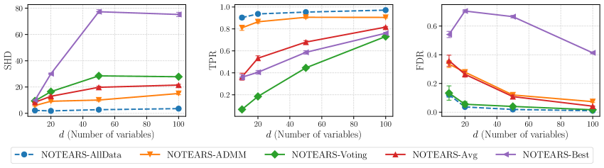
Figure 1: Structure learning results of linear Gaussian BNs with varying number of variables. There are $n=3d$ samples in total, distributed evenly across $K=10$ clients. Error bars refer to the standard errors computed over $30$ random runs.

6 Experiments

We conduct empirical studies to verify the effectiveness of the proposed federated BNSL approach. In Sections 6.1 and 6.2, we provide experimental results with varying number of variables and clients, respectively. We then apply the proposed approach to real data in Section 6.3, and to the nonlinear case in Section 6.4.

Simulations.    The true DAGs are simulated using the Erdös–Rényi (Erdös and Rényi, 1959) model with number of edges equal to the number of variables $d$. In the linear case, we follow Zheng et al. (2018) and generate the data according to the linear Gaussian BNs, in which the coefficients are sampled uniformly at random from $[-2,-0.5]\cup[0.5,2]$, and the noise terms are standard Gaussian. In the nonlinear case, similar to (Zheng et al., 2020), we simulate the nonlinear BNs with each function being a randomly initialized MLP consisting of one hidden layer and $100$ sigmoid activation units. The structures of these two data models are fully identifiable (Peters and Bühlmann, 2013; Peters et al., 2014). We focus on the setting in which each client has a limited sample size, which may in practice be the reason why the clients intend to collaborate.

Methods.    In the linear case, we compare the ADMM approach described in Section 5.1, denoted as NOTEARS-ADMM, to the voting approach proposed by Na and Yang (2010), denoted as NOTEARS-Voting. In particular, we apply the NOTEARS (Zheng et al., 2018) method to estimate the DAG from each client’s local dataset independently, and use a voting scheme that picks those edges identified by more than half of the clients. We also include another baseline that computes the average of the weighted adjacency matrices estimated by NOTEARS from the local datasets, and then perform thresholding to identify the edges, which we denote by NOTEARS-Avg. Apart from voting and averaging, we adopt another baseline that picks the best graph, i.e., with the lowest structural Hamming distance (SHD), from the independently estimated graphs by the clients, denoted as NOTEARS-Best. In practice, the ground truth may not be known, and we are not able to pick the best graph in such a way; however, this serves as a reasonable baseline to our approach. Also, note that the final graph returned by NOTEARS-Voting and NOTEARS-Avg may contain cycles, but we do not apply any post-processing step to remove them as it may worsen the performance. We also report the performance of NOTEARS on all data by combining all clients’ local datasets, denoted by NOTEARS-AllData. Similarly, in the nonlinear case, we compare among NOTEARS-MLP-ADMM, NOTEARS-MLP-Voting, NOTEARS-MLP-Avg, NOTEARS-MLP-Best, and NOTEARS-MLP-AllData.

Following Zheng et al. (2018, 2020), a thresholding step at $0.3$ is used to remove the estimated edges with small weights. Further implementation details and hyperparameters of the proposed approach are described in Appendix B. The code is available at https://github.com/ignavierng/notears-admm.

Metrics.    We use the SHD, true positive rate (TPR), and false discovery rate (FDR) to evaluate the estimated graphs, computed over $30$ random runs.

6.1 Varying Number of Variables

We consider the linear Gaussian BNs with a total number of $n=3d$ samples distributed evenly across $K=10$ clients, i.e., each client has $\left\lfloor 0.3d\right\rfloor$ samples. We conduct experiments with $d\in\{10,20,50,100\}$ variables.

The results are shown in Figure 1. One observes that NOTEARS-ADMM performs the best across different number of variables, and the difference of SHD grows as the number of variables increases. It also has relatively high TPRs which are close to those of NOTEARS-AllData, compared to the other baselines, indicating that it manages to identify most of the edges. Among the baselines, NOTEARS-Avg has lower SHDs than NOTEARS-Voting as the latter identifies only a small number of edges, leading to low TPRs. Notice that NOTEARS-Best has high SHDs owing to high FDRs. A possible reason is that the sample size is too small which gives rise to a high estimation error.

Other baselines.    We also consider BNSL methods that are not based on continuous optimization. In particular, we apply the voting scheme to the structures independently estimated by PC (Spirtes and Glymour, 1991) and FGES (Ramsey et al., 2017) from the clients’ local datasets, denoted as PC-Voting and FGES-Voting. Since these methods output the Markov equivalence classes instead of DAGs, we follow Zheng et al. (2018) and consider each undirected edge as a true positive if there is a directed edge in place of the undirected one in the true DAG. The results are reported in Figure 5 in Appendix C, showing that these methods have worse SHDs and TPRs than those of NOTEARS-ADMM.

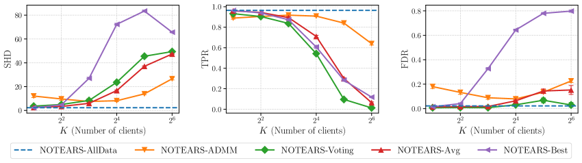
Figure 2: Structure learning results of linear Gaussian BNs with $d=50$ variables and varying number of clients. There are $n=256$ samples in total, distributed evenly across $K\in\{2,4,8,16,32,64\}$ clients. Error bars refer to the standard errors computed over $30$ random runs.

6.2 Varying Number of Clients

We now consider a fixed total number of samples which are distributed across different number of clients. For $d\in\{10,20,50\}$ variables, we generate $n=256$ samples and distribute them across $K\in\{2,4,8,16,32,64\}$ clients. This may be a challenging setup because, for, e.g., $K=64$ clients, each client has only $4$ samples.

Figure 2 shows the results with $50$ variables, while those with $d\in\{10,20\}$ variables are depicted by Figure 6 in Appendix C owing to space limit. As the number of clients $K$ increases, the TPRs of NOTEARS-Voting, NOTEARS-Avg, and NOTEARS-Best quickly deteriorate, leading to high SHDs. On the other hand, although the TPRs of NOTEARS-ADMM also decrease with a larger $K$, they are still relatively high as compared to those of the other baselines. For instance, with $d=20$ variables and $K=64$ clients, NOTEARS-ADMM achieves a TPR of $0.78$, while NOTEARS-Voting, NOTEARS-Avg, and NOTEARS-Best have TPRs of $0.05$, $0.25$, and $0.33$, respectively. This verifies the effectiveness of NOTEARS-ADMM in the setting with a large number of (up to $64$) clients and indicates that exchanging information during the optimization process is a key to learning an accurate BN structure, as is the case for NOTEARS-ADMM. On the contrary, the other baselines utilize only the information of the independently estimated DAGs by the clients, and therefore the information exchange is rather limited.

Interestingly, when the number of clients $K$ is small, the other baselines perform better than NOTEARS-ADMM. For instance, with $50$ variables, NOTEARS-Voting, NOTEARS-Avg, and NOTEARS-Best have better SHDs than NOTEARS-ADMM when there are only $2$ or $4$ clients. This is not surprising because for a small number of clients $K$, the sample size may be sufficient for each client to independently learn an accurate enough BN structure, i.e., $n=128,64$ samples for $K=2,4$ clients, respectively. On the other hand, NOTEARS-ADMM involves solving a more complex nonconvex optimization problem, and therefore the solutions obtained may not be as accurate as those by the baselines especially when the task is relatively easy, i.e., each client has a sufficient sample size and is able to learn an accurate enough BN structure on their own.

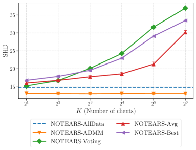
Figure 3: Real data with $512$ samples in total, distributed evenly across $K\in\{2,4,8,16,32,64\}$ clients.

6.3 Real Data

We evaluate the proposed method on a protein expression dataset from Sachs et al. (2005). This dataset contains $n=853$ observational samples and $11$ variables, and the proposed ground truth DAG contains $17$ edges. For each of the $30$ random runs, we randomly pick $n=512$ samples from the dataset and distribute them across $K\in\{2,4,8,16,32,64\}$ clients, in order to simulate a setting in which the real data is distributed across different parties.

The SHDs are shown in Figure 3, while the complete results including TPRs and FDRs are reported in Figure 7 in Appendix C. Similar to the empirical study in Section 6.2, we observe here that the performance of NOTEARS-Voting, NOTEARS-Avg, and NOTEARS-Best degrades much as the number of clients increases, whereas NOTEARS-ADMM has an improved and stable performance across different number of clients. This indicates that NOTEARS-ADMM is relatively robust in practice even when there is a large number of clients and each has a small sample size. It is interesting to observe that NOTEARS-ADMM has lower SHDs than those of NOTEARS-AllData, possibly because of the model misspecification on this real dataset.

6.4 Nonlinear Case

We now provide empirical results in the nonlinear case to demonstrate the flexibility of the proposed approach. Similar to Section 6.2, we simulate $512$ samples using the nonlinear BNs with MLPs, in which the ground truths have $50$ variables, and distribute these samples across $K\in\{2,4,8,16\}$ clients. We did not include the experiments for $32$ and $64$ clients as the running time of some of the baselines may be too long.

Due to space limit, we report the SHDs in Figure 4 and the complete results in Figure 8 in Appendix C. Consistent with previous observations, NOTEARS-MLP-ADMM outperforms the other baselines and has a much stable performance across different number of clients, which is close to that of NOTEARS-MLP-AllData. This demonstrates the effectiveness of our approach in the nonlinear case, and validates the importance of information exchange during the optimization.

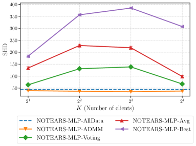
Figure 4: Nonlinear BNs with $512$ samples in total, distributed evenly across $K\in\{2,4,8,16\}$ clients.

7 Discussion

We presented a federated learning approach to carry out BNSL from horizontally partitioned data. In particular, we developed a distributed BNSL method based on ADMM such that only the model parameters have to be exchanged during the optimization process. The proposed approach is flexible and can be adopted for both linear and nonlinear cases. Our experiments show that it achieves an improved performance over the other methods, especially when there is a relatively large number of clients and each has a small sample size, which is typical in the federated learning setting and may in practice be the reason why the clients intend to collaborate. We discuss below some limitations of the proposed approach and possible directions for future work. We hope that this work could spur future studies on developing federated approaches for BNSL.

More complex settings.    As described in Section 2.1, continuous optimization methods for BNSL have been extended to different settings, such as those with confounders (Bhattacharya et al., 2020) and interventional data (Brouillard et al., 2020). Furthermore, the data distribution of different clients may, in practice, be heterogenous. An important direction is to extend the proposed approach to these settings.

Federated optimization.    The proposed approach with ADMM is stateful and requires each client to participate in each round of communication, and therefore is only suitable for the cross-silo setting, in which the clients usually refer to different organizations or companies. An important direction for future is to explore the use of other federated optimization techniques such as federated averaging (McMahan et al., 2017) that allow for stateless clients and cross-device learning.

Convergence properties.    Some recent works have studied the convergence of ADMM in the nonconvex setting (Hong et al., 2014; Wang et al., 2019), and of the continuous constrained formulation of BNSL (Wei et al., 2020; Ng et al., 2022a). The latter showed that the regularity condition required by standard convergence results of augmented Lagrangian method is not satisfied, and thus its behavior is similar to that of the quadratic penalty method (Powell, 1969; Fletcher, 1987), another class of algorithm for solving constrained optimization problem. It is an interesting future direction to investigate whether similar convergence properties hold for our approach with ADMM.

Vertically partitioned data.    In practice, the data may be vertically partitioned across different clients, i.e., they may own different variables and wish to collectively carry out BNSL. Therefore, it can be useful to develop a federated approach for the vertical setting. A related setting is to estimate structures from overlapping variables; see a review in Section 2.2.

Privacy protection.    The proposed ADMM procedure involves sharing the model parameters with the central server. Therefore, another important direction is to investigate how much information the model parameters may leak, because they have been shown to possibly leak some information in certain cases, e.g., image data (Phong et al., 2018). It is also interesting to consider the use of differential privacy (Dwork and Roth, 2014) or homomorphic encryption, e.g., the Paillier’s scheme (Paillier, 1999), for further privacy protection of the model parameters.

Appendix A Derivation of Closed-Form Solution

For completeness, in this section we derive the closed-form solution of the subproblem (4) for our ADMM approach in the linear case. We drop the superscript $t$ to lighten the notation, which leads to the optimization problem

$$\min_{B_{k}}\ \ f(B_{k})\coloneqq\ell(B_{k};\mathbf{x}_{k})+\operatorname{tr}\left(\beta_{k}(B_{k}-W)^{\mathsf{T}}\right)+\frac{\rho_{2}}{2}\|B_{k}-W\|_{F}^{2}.$$

This is known as a proximal minimization problem and is well studied in the literature of numerical optimization (Combettes and Pesquet, 2011; Parikh and Boyd, 2014). With a slight abuse of notation, let $\mathbf{x}_{k}\in\mathbb{R}^{n_{k}\times d}$ denote the design matrix that corresponds to the samples of the $k$-th client. Also let $S_{k}=(1/n)\mathbf{x}_{k}^{\mathsf{T}}\mathbf{x}_{k}$. The first term of the function $f(B_{k})$ can be written as

$$\ell(B_{k};\mathbf{x}_{k}) =\frac{1}{2n}\|\mathbf{x}_{k}-\mathbf{x}_{k}B_{k}\|_{F}^{2}$$

$$=\frac{1}{2n}\operatorname{tr}\left((\mathbf{x}_{k}-\mathbf{x}_{k}B_{k})^{\mathsf{T}}(\mathbf{x}_{k}-\mathbf{x}_{k}B_{k})\right)$$

$$=\frac{1}{2n}\operatorname{tr}\left(\mathbf{x}_{k}^{\mathsf{T}}\mathbf{x}_{k}-B_{k}^{\mathsf{T}}\mathbf{x}_{k}^{\mathsf{T}}\mathbf{x}_{k}-\mathbf{x}_{k}^{\mathsf{T}}\mathbf{x}_{k}B_{k}+B_{k}^{\mathsf{T}}\mathbf{x}_{k}^{\mathsf{T}}\mathbf{x}_{k}B_{k}\right)$$

$$=\frac{1}{2}\operatorname{tr}\left(S_{k}-B_{k}^{\mathsf{T}}S_{k}-S_{k}B_{k}+B_{k}^{\mathsf{T}}S_{k}B_{k}\right)$$

$$=\frac{1}{2}\operatorname{tr}\left(S_{k}-2B_{k}^{\mathsf{T}}S_{k}+B_{k}^{\mathsf{T}}S_{k}B_{k}\right),$$

where the last line follows from $S_{k}$ being symmetric. Similarly, the third term of function $f(B_{k})$ can be written as

$$\frac{\rho_{2}}{2}\|B_{k}-W\|_{F}^{2} =\frac{\rho_{2}}{2}\operatorname{tr}\left((B_{k}-W)^{\mathsf{T}}(B_{k}-W)\right)$$

$$=\frac{\rho_{2}}{2}\operatorname{tr}\left(B_{k}^{\mathsf{T}}B_{k}-2B_{k}^{\mathsf{T}}W+W^{\mathsf{T}}W\right).$$

Therefore, we have

$$f(B_{k}) =\frac{1}{2}\operatorname{tr}\left(S_{k}-2B_{k}^{\mathsf{T}}S_{k}+B_{k}^{\mathsf{T}}S_{k}B_{k}\right)+\operatorname{tr}\left(\beta_{k}B_{k}^{\mathsf{T}}-\beta_{k}W^{\mathsf{T}}\right)+\frac{\rho_{2}}{2}\operatorname{tr}\left(B_{k}^{\mathsf{T}}B_{k}-2B_{k}^{\mathsf{T}}W+W^{\mathsf{T}}W\right)$$

$$=\operatorname{tr}\left(\frac{1}{2}B_{k}^{\mathsf{T}}\left(S_{k}+\rho_{2}I\right)B_{k}-B_{k}^{\mathsf{T}}(\rho_{2}W-\beta_{k}+S_{k})\right)+\text{const},$$

and its derivative is given by

$$\nabla_{B_{k}}f(B_{k}) =\frac{1}{2}\left(\left(S_{k}+\rho_{2}I\right)^{\mathsf{T}}+\left(S_{k}+\rho_{2}I\right)\right)B_{k}-(\rho_{2}W-\beta_{k}+S_{k})$$

$$=(S_{k}+\rho_{2}I)B_{k}-(\rho_{2}W-\beta_{k}+S_{k}).$$

By definition, we have $\rho_{2}>0$, which implies that the matrix $S_{k}+\rho_{2}I$ is symmetric positive definite, and therefore is invertible. Solving $\nabla_{B_{k}}f(B_{k})=0$ yields the solution

$$B_{k}^{*}=(S_{k}+\rho_{2}I)^{-1}(\rho_{2}W-\beta_{k}+S_{k}).$$

Since the matrix $(1/2)(S_{k}+\rho_{2}I)$ is symmetric positive definite, the function $f(B_{k})$ is strictly convex, indicating that $B_{k}^{*}$ is its unique global minimum.

Appendix B Implementation Details and Hyperparameters

Implementation details.    The proposed distributed BNSL approach with ADMM is implemented with PyTorch (Paszke et al., 2019). In both linear and nonlinear cases (corresponding to NOTEARS-ADMM and NOTEARS-MLP-ADMM, respectively), we follow Zheng et al. (2018, 2020) and use the L-BFGS method (Byrd et al., 2003) to solve the unconstrained optimization problem in the augmented Lagrangian method, except for problem (4), for which a closed-form solution exists. To handle the $\ell_{1}$ penalty term, we use the subgradient method (Stephen Boyd, 2003) to simplify our procedure, instead of the bound-constrained formulation adopted by Zheng et al. (2018, 2020). After the optimization process of ADMM finishes, we use the final solution of the global variable $W$ as our estimated model function, which corresponds to the linear coefficients and MLP parameters in the linear and nonlinear cases, respectively. For the linear case, the linear coefficients directly represent the weighted adjacency matrix, while for the nonlinear case, similar procedure described by Zheng et al. (2020) is used to construct the equivalent weighted adjacency matrix. We then perform thresholding at $0.3$ to obtain the final estimated structure.

Hyperparameters.    We set $\gamma_{1}$ and $\gamma_{2}$ to $1.75$ and $1.25$, respectively. The initial estimations of the Lagrange multipliers $\alpha^{1}$ and $\beta_{1}^{1},\dots,\beta_{K}^{1}$ are set to zero and zero matrices, respectively. For the initial penalty coefficients and $\ell_{1}$ regularization coefficient, we find that $\rho_{1}^{1}=\rho_{2}^{1}=0.001$ and $\lambda=0.01$ work well in the linear case, while $\rho_{1}^{1}=\rho_{2}^{1}=0.1$ and $\lambda=0.001$ work well in the nonlinear case. We also set the maximum number of augmented Lagrangian iterations to $200$, and the maximum penalty coefficients to $1\times 10^{16}$. These values are selected using small-scale experiments with $d=30$ variables and $K=8$ clients.

Appendix C Supplementary Experimental Results

This section provides additional empirical results for Section 6, as shown in Figures 5, 6, 7, and 8.

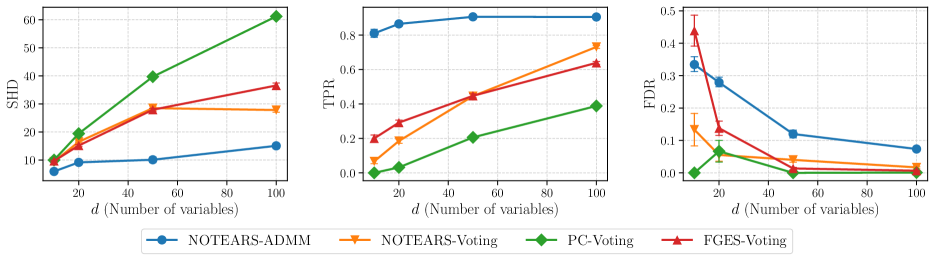
Figure 5: Structure learning results of linear Gaussian BNs with varying number of variables. There are $n=3d$ samples in total, distributed evenly across $K=10$ clients. BNSL methods that are not based on continuous optimization are included, i.e., PC-Voting and FGES-Voting. Error bars refer to the standard errors computed over $30$ random runs.

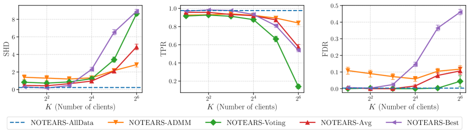
(a) 10 variables.

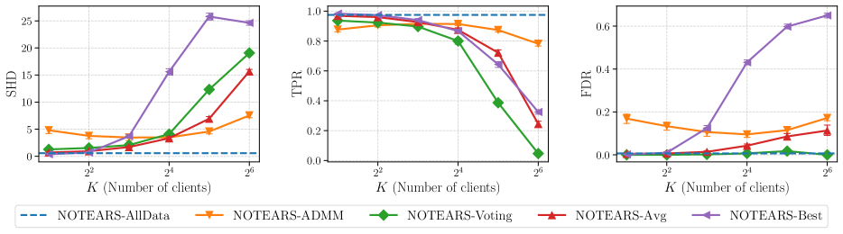
(b) 20 variables.

Figure 6: Structure learning results of linear Gaussian BNs with varying number of clients. There are $n=256$ samples in total, distributed evenly across $K\in\{2,4,8,16,32,64\}$ clients. Error bars refer to the standard errors computed over $30$ random runs.

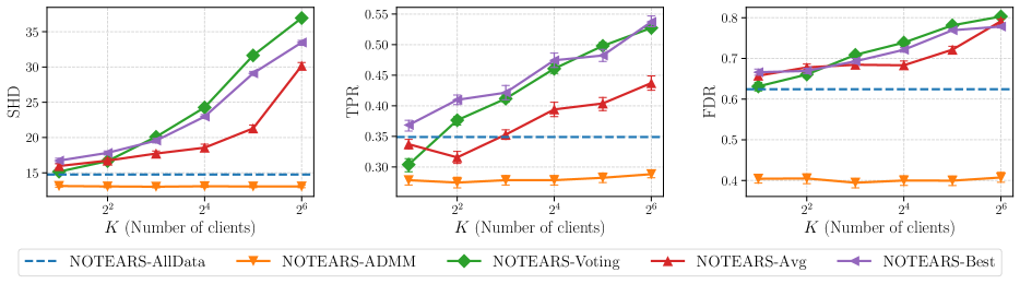
Figure 7: Structure learning results of a real dataset with varying number of clients. There are $n=512$ samples in total, distributed evenly across $K\in\{2,4,8,16,32,64\}$ clients. Error bars refer to the standard errors computed over $30$ random runs.

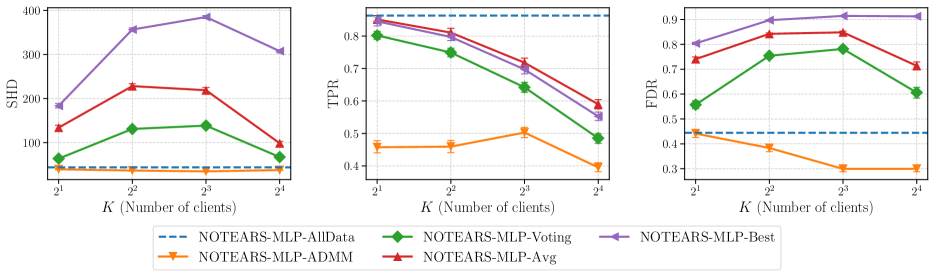
Figure 8: Structure learning results of nonlinear BNs with $d=50$ variables and varying number of clients. There are $n=512$ samples in total, distributed evenly across $K\in\{2,4,8,16\}$ clients. Error bars refer to the standard errors computed over $30$ random runs.

References

- Ács and Castelluccia (2011) G. Ács and C. Castelluccia. I have a dream! (differentially private smart metering). In Information Hiding, 2011.
- Aragam et al. (2019) B. Aragam, A. Amini, and Q. Zhou. Globally optimal score-based learning of directed acyclic graphs in high-dimensions. In Advances in Neural Information Processing Systems, volume 32, 2019.
- Bertsekas (1982) D. P. Bertsekas. Constrained Optimization and Lagrange Multiplier Methods. Academic Press, 1982.
- Bertsekas (1999) D. P. Bertsekas. Nonlinear Programming. Athena Scientific, 2nd edition, 1999.
- Bertsekas and Tsitsiklis (1989) D. P. Bertsekas and J. N. Tsitsiklis. Parallel and Distributed Computation: Numerical Methods. Prentice-Hall, Inc., 1989.
- Bhattacharya et al. (2020) R. Bhattacharya, T. Nagarajan, D. Malinsky, and I. Shpitser. Differentiable causal discovery under unmeasured confounding. arXiv preprint arXiv:2010.06978, 2020.
- Boyd et al. (2011) S. Boyd, N. Parikh, E. Chu, B. Peleato, and J. Eckstein. Distributed optimization and statistical learning via the alternating direction method of multipliers. Foundations and Trends in Machine Learning, 3(1):1–122, 2011.
- Brouillard et al. (2020) P. Brouillard, S. Lachapelle, A. Lacoste, S. Lacoste-Julien, and A. Drouin. Differentiable causal discovery from interventional data. In Advances in Neural Information Processing Systems, 2020.
- Burkhart et al. (2010) M. Burkhart, M. Strasser, D. Many, and X. Dimitropoulos. SEPIA: Privacy-preserving aggregation of multi-domain network events and statistics. In 19th USENIX Security Symposium (USENIX Security 10). USENIX Association, 08 2010.
- Byrd et al. (2003) R. Byrd, P. Lu, J. Nocedal, and C. Zhu. A limited memory algorithm for bound constrained optimization. SIAM Journal on Scientific Computing, 16, 2003.
- Chai et al. (2020) D. Chai, L. Wang, K. Chen, and Q. Yang. Secure federated matrix factorization. IEEE Intelligent Systems, (01), 08 2020.
- Chen et al. (2003) R. Chen, K. Sivakumar, and H. Khargupta. Learning Bayesian network structure from distributed data. In SIAM International Conference on Data Mining, 2003.
- Chickering (2002) D. M. Chickering. Optimal structure identification with greedy search. Journal of Machine Learning Research, 3(Nov):507–554, 2002.
- Clifton et al. (2002) C. Clifton, M. Kantarcioglu, J. Vaidya, X. Lin, and M. Y. Zhu. Tools for privacy preserving distributed data mining. ACM SIGKDD Explorations Newsletter, 4(2):28–34, 12 2002.
- Combettes and Pesquet (2011) P. L. Combettes and J.-C. Pesquet. Proximal Splitting Methods in Signal Processing, pages 185–212. Springer New York, 2011.
- Cussens (2011) J. Cussens. Bayesian network learning with cutting planes. In Conference on Uncertainty in Artificial Intelligence, 2011.
- Danks et al. (2008) D. Danks, C. Glymour, and R. Tillman. Integrating locally learned causal structures with overlapping variables. In Advances in Neural Information Processing Systems, 2008.
- Dwork and Roth (2014) C. Dwork and A. Roth. The algorithmic foundations of differential privacy. Foundations and Trends® in Theoretical Computer Science, 9(3–4):211–407, 2014.
- Erdös and Rényi (1959) P. Erdös and A. Rényi. On random graphs I. Publicationes Mathematicae, 6:290–297, 1959.
- Fletcher (1987) R. Fletcher. Practical Methods of Optimization. Wiley-Interscience, 1987.
- Gabay and Mercier (1976) D. Gabay and B. Mercier. A dual algorithm for the solution of nonlinear variational problems via finite element approximation. Computers & Mathematics With Applications, 2:17–40, 1976.
- Glowinski and Marroco (1975) R. Glowinski and A. Marroco. Sur l’approximation, par éléments finis d’ordre un, et la résolution, par pénalisation-dualité d’une classe de problèmes de Dirichlet non linéaires. ESAIM: Mathematical Modelling and Numerical Analysis - Modélisation Mathématique et Analyse Numérique, 9(R2):41–76, 1975.
- Goryczka and Xiong (2017) S. Goryczka and L. Xiong. A comprehensive comparison of multiparty secure additions with differential privacy. IEEE transactions on dependable and secure computing, 14(5):463–477, 2017.
- Gou et al. (2007) K. X. Gou, G. X. Jun, and Z. Zhao. Learning Bayesian network structure from distributed homogeneous data. In ACIS International Conference on Software Engineering, Artificial Intelligence, Networking, and Parallel/Distributed Computing, volume 3, pages 250–254, 2007.
- Hazay et al. (2017) C. Hazay, G. L. Mikkelsen, T. Rabin, T. Toft, and A. A. Nicolosi. Efficient RSA key generation and threshold Paillier in the two-party setting. Journal of Cryptology, 32:265–323, 2017.
- Hong et al. (2014) M. Hong, Z.-Q. Luo, and M. Razaviyayn. Convergence analysis of alternating direction method of multipliers for a family of nonconvex problems. SIAM Journal on Optimization, 26, 10 2014.
- Huang et al. (2018) B. Huang, K. Zhang, Y. Lin, B. Schölkopf, and C. Glymour. Generalized score functions for causal discovery. In Proceedings of the 24th ACM SIGKDD International Conference on Knowledge Discovery & Data Mining, 2018.
- Huang et al. (2020) B. Huang, K. Zhang, M. Gong, and C. Glymour. Causal discovery from multiple data sets with non-identical variable sets. In Proceedings of the AAAI Conference on Artificial Intelligence, 2020.
- Jang et al. (2017) E. Jang, S. Gu, and B. Poole. Categorical reparameterization with Gumbel-Softmax. In International Conference on Learning Representations, 2017.
- Kairouz et al. (2021) P. Kairouz, H. B. McMahan, B. Avent, A. Bellet, M. Bennis, A. N. Bhagoji, K. Bonawitz, Z. Charles, G. Cormode, R. Cummings, R. G. L. D’Oliveira, H. Eichner, S. E. Rouayheb, D. Evans, J. Gardner, Z. Garrett, A. Gascón, B. Ghazi, P. B. Gibbons, M. Gruteser, Z. Harchaoui, C. He, L. He, Z. Huo, B. Hutchinson, J. Hsu, M. Jaggi, T. Javidi, G. Joshi, M. Khodak, J. Konecný, A. Korolova, F. Koushanfar, S. Koyejo, T. Lepoint, Y. Liu, P. Mittal, M. Mohri, R. Nock, A. Özgür, R. Pagh, H. Qi, D. Ramage, R. Raskar, M. Raykova, D. Song, W. Song, S. U. Stich, Z. Sun, A. T. Suresh, F. Tramèr, P. Vepakomma, J. Wang, L. Xiong, Z. Xu, Q. Yang, F. X. Yu, H. Yu, and S. Zhao. Advances and open problems in federated learning. Foundations and Trends in Machine Learning, 14(1–2):1–210, 2021.
- Kalainathan et al. (2018) D. Kalainathan, O. Goudet, I. Guyon, D. Lopez-Paz, and M. Sebag. Structural agnostic modeling: Adversarial learning of causal graphs. arXiv preprint arXiv:1803.04929, 2018.
- Koller and Friedman (2009) D. Koller and N. Friedman. Probabilistic Graphical Models: Principles and Techniques. MIT Press, Cambridge, MA, 2009.
- Lachapelle et al. (2020) S. Lachapelle, P. Brouillard, T. Deleu, and S. Lacoste-Julien. Gradient-based neural DAG learning. In International Conference on Learning Representations, 2020.
- Li et al. (2020) T. Li, A. K. Sahu, A. S. Talwalkar, and V. Smith. Federated learning: Challenges, methods, and future directions. IEEE Signal Processing Magazine, 37:50–60, 2020.
- Lucas et al. (2004) P. J. F. Lucas, L. C. van der Gaag, and A. Abu-Hanna. Bayesian networks in biomedicine and healthcare. Artificial Intelligence in Medicine, 30(3):201–214, 2004.
- McMahan et al. (2017) B. McMahan, E. Moore, D. Ramage, S. Hampson, and B. A. y. Arcas. Communication-efficient learning of deep networks from decentralized data. In International Conference on Artificial Intelligence and Statistics, 2017.
- Meinshausen and Bühlmann (2006) N. Meinshausen and P. Bühlmann. High-dimensional graphs and variable selection with the Lasso. The Annals of Statistics, 34:1436–1462, 2006.
- Na and Yang (2010) Y. Na and J. Yang. Distributed Bayesian network structure learning. In IEEE International Symposium on Industrial Electronics, pages 1607–1611, 2010.
- Ng et al. (2019) I. Ng, S. Zhu, Z. Chen, and Z. Fang. A graph autoencoder approach to causal structure learning. arXiv preprint arXiv:1911.07420, 2019.
- Ng et al. (2020) I. Ng, A. Ghassami, and K. Zhang. On the role of sparsity and DAG constraints for learning linear DAGs. In Advances in Neural Information Processing Systems, 2020.
- Ng et al. (2022a) I. Ng, S. Lachapelle, N. R. Ke, S. Lacoste-Julien, and K. Zhang. On the convergence of continuous constrained optimization for structure learning. In International Conference on Artificial Intelligence and Statistics, 2022a.
- Ng et al. (2022b) I. Ng, S. Zhu, Z. Fang, H. Li, Z. Chen, and J. Wang. Masked gradient-based causal structure learning. In SIAM International Conference on Data Mining, 2022b.
- Paillier (1999) P. Paillier. Public-key cryptosystems based on composite degree residuosity classes. In International Conference on the Theory and Applications of Cryptographic Techniques, 1999.
- Pamfil et al. (2020) R. Pamfil, N. Sriwattanaworachai, S. Desai, P. Pilgerstorfer, P. Beaumont, K. Georgatzis, and B. Aragam. DYNOTEARS: Structure learning from time-series data. In International Conference on Artificial Intelligence and Statistics, 2020.
- Parikh and Boyd (2014) N. Parikh and S. Boyd. Proximal algorithms. Foundations and Trends in Optimization, 1(3):127–239, 01 2014.
- Paszke et al. (2019) A. Paszke, S. Gross, F. Massa, A. Lerer, J. Bradbury, G. Chanan, T. Killeen, Z. Lin, N. Gimelshein, L. Antiga, A. Desmaison, A. Kopf, E. Yang, Z. DeVito, M. Raison, A. Tejani, S. Chilamkurthy, B. Steiner, L. Fang, J. Bai, and S. Chintala. PyTorch: An imperative style, high-performance deep learning library. In Advances in Neural Information Processing Systems, 2019.
- Pearl (2009) J. Pearl. Causality: Models, Reasoning and Inference. Cambridge University Press, 2009.
- Peters and Bühlmann (2013) J. Peters and P. Bühlmann. Identifiability of Gaussian structural equation models with equal error variances. Biometrika, 101(1):219–228, 2013.
- Peters et al. (2014) J. Peters, J. M. Mooij, D. Janzing, and B. Schölkopf. Causal discovery with continuous additive noise models. Journal of Machine Learning Research, 15(1):2009–2053, 2014.
- Peters et al. (2017) J. Peters, D. Janzing, and B. Schölkopf. Elements of Causal Inference - Foundations and Learning Algorithms. MIT Press, 2017.
- Phong et al. (2018) L. T. Phong, Y. Aono, T. Hayashi, L. Wang, and S. Moriai. Privacy-preserving deep learning via additively homomorphic encryption. IEEE Transactions on Information Forensics and Security, 13(5):1333–1345, 2018.
- Powell (1969) M. J. D. Powell. Nonlinear programming—sequential unconstrained minimization techniques. The Computer Journal, 12(3), 1969.
- Ramsey et al. (2017) J. Ramsey, M. Glymour, R. Sanchez-Romero, and C. Glymour. A million variables and more: the fast greedy equivalence search algorithm for learning high-dimensional graphical causal models, with an application to functional magnetic resonance images. International Journal of Data Science and Analytics, 3(2):121–129, 2017.
- Reddi et al. (2021) S. J. Reddi, Z. Charles, M. Zaheer, Z. Garrett, K. Rush, J. Konečný, S. Kumar, and H. B. McMahan. Adaptive federated optimization. In International Conference on Learning Representations, 2021.
- Runge et al. (2019) J. Runge, S. Bathiany, E. Bollt, G. Camps-Valls, D. Coumou, E. Deyle, C. Glymour, M. Kretschmer, M. Mahecha, J. Muñoz-Marí, E. V. van Nes, J. Peters, R. Quax, M. Reichstein, M. Scheffer, B. Schölkopf, P. Spirtes, G. Sugihara, J. Sun, K. Zhang, and J. Zscheischler. Inferring causation from time series in Earth system sciences. Nature Communications, 10, 2019.
- Sachs et al. (2005) K. Sachs, O. Perez, D. Pe’er, D. A. Lauffenburger, and G. P. Nolan. Causal protein-signaling networks derived from multiparameter single-cell data. Science, 308(5721):523–529, 2005.
- Samet and Miri (2009) S. Samet and A. Miri. Privacy-preserving Bayesian network for horizontally partitioned data. In International Conference on Computational Science and Engineering, volume 3, pages 9–16, 2009.
- Schmidt et al. (2007) M. Schmidt, A. Niculescu-Mizil, and K. Murphy. Learning graphical model structure using L1-regularization paths. In Proceedings of the 22nd National Conference on Artificial Intelligence - Volume 2, pages 1278–1283. AAAI Press, 2007.
- Schwarz (1978) G. Schwarz. Estimating the dimension of a model. The Annals of Statistics, 6(2):461–464, 1978.
- Shamir (1979) A. Shamir. How to share a secret. Communications of the ACM, 22(11):612–613, 11 1979.
- Shi et al. (2011) E. Shi, T.-H. H. Chan, E. G. Rieffel, R. Chow, and D. Song. Privacy-preserving aggregation of time-series data. In Proceedings of the Network and Distributed System Security Symposium. The Internet Society, 2011.
- Shimizu et al. (2006) S. Shimizu, P. O. Hoyer, A. Hyvärinen, and A. Kerminen. A linear non-Gaussian acyclic model for causal discovery. Journal of Machine Learning Research, 7(Oct):2003–2030, 2006.
- Singh and Moore (2005) A. P. Singh and A. W. Moore. Finding optimal Bayesian networks by dynamic programming. Technical report, Carnegie Mellon University, 2005.
- Spirtes and Glymour (1991) P. Spirtes and C. Glymour. An algorithm for fast recovery of sparse causal graphs. Social Science Computer Review, 9:62–72, 1991.
- Spirtes et al. (2001) P. Spirtes, C. Glymour, and R. Scheines. Causation, Prediction, and Search. MIT press, 2nd edition, 2001.
- Stephen Boyd (2003) A. M. Stephen Boyd, Lin Xiao. Subgradient methods, February 2003.
- Tillman and Eberhardt (2014) R. E. Tillman and F. Eberhardt. Learning causal structure from multiple datasets with similar variable sets. Behaviormetrika, 41:41–64, 2014.
- Triantafillou and Tsamardinos (2015) S. Triantafillou and I. Tsamardinos. Constraint-based causal discovery from multiple interventions over overlapping variable sets. Journal of Machine Learning Research, 16(66):2147–2205, 2015.
- Triantafillou et al. (2010) S. Triantafillou, I. Tsamardinos, and I. Tollis. Learning causal structure from overlapping variable sets. In International Conference on Artificial Intelligence and Statistics, 2010.
- Van de Geer and Bühlmann (2013) S. Van de Geer and P. Bühlmann. -penalized maximum likelihood for sparse directed acyclic graphs. The Annals of Statistics, 41(2):536–567, 2013.
- Wang et al. (2019) Y. Wang, W. Yin, and J. Zeng. Global convergence of ADMM in nonconvex nonsmooth optimization. Journal of Scientific Computing, 78(1):29–63, 01 2019.
- Wei et al. (2020) D. Wei, T. Gao, and Y. Yu. DAGs with no fears: A closer look at continuous optimization for learning Bayesian networks. In Advances in Neural Information Processing Systems, 2020.
- Wright and Yang (2004) R. Wright and Z. Yang. Privacy-preserving Bayesian network structure computation on distributed heterogeneous data. In Proceedings of the Tenth ACM SIGKDD International Conference on Knowledge Discovery and Data Mining, 2004.
- Yang et al. (2019) Q. Yang, Y. Liu, T. Chen, and Y. Tong. Federated machine learning: Concept and applications. ACM Transactions on Intelligent Systems and Technology, 10(2), 01 2019.
- Yang and Wright (2006) Z. Yang and R. Wright. Privacy-preserving computation of Bayesian networks on vertically partitioned data. IEEE Transactions on Knowledge and Data Engineering, 18(9):1253–1264, 2006.
- Yu et al. (2019) Y. Yu, J. Chen, T. Gao, and M. Yu. DAG-GNN: DAG structure learning with graph neural networks. In International Conference on Machine Learning, 2019.
- Yu et al. (2021) Y. Yu, T. Gao, N. Yin, and Q. Ji. DAGs with no curl: An efficient DAG structure learning approach. In International Conference on Machine Learning, 2021.
- Zhang et al. (2020) C. Zhang, S. Li, J. Xia, W. Wang, F. Yan, and Y. Liu. Batchcrypt: Efficient homomorphic encryption for cross-silo federated learning. In USENIX Annual Technical Conference, 2020.
- Zhang et al. (2012) K. Zhang, J. Peters, D. Janzing, and B. Schölkopf. Kernel-based conditional independence test and application in causal discovery. In Conference on Uncertainty in Artificial Intelligence, 2012.
- Zheng et al. (2018) X. Zheng, B. Aragam, P. Ravikumar, and E. P. Xing. DAGs with NO TEARS: Continuous optimization for structure learning. In Advances in Neural Information Processing Systems, 2018.
- Zheng et al. (2020) X. Zheng, C. Dan, B. Aragam, P. Ravikumar, and E. P. Xing. Learning sparse nonparametric DAGs. In International Conference on Artificial Intelligence and Statistics, 2020.
Supplementary Material:
Towards Federated Bayesian Network Structure Learning with Continuous Optimization