FAST3D: Flow-Aware Self-Training for 3D Object Detectors

Abstract

In the field of autonomous driving, self-training is widely applied to mitigate distribution shifts in LiDAR-based 3D object detectors. This eliminates the need for expensive, high-quality labels whenever the environment changes (e.g, geographic location, sensor setup, weather condition). State-of-the-art self-training approaches, however, mostly ignore the temporal nature of autonomous driving data.

To address this issue, we propose a flow-aware self-training method which enables unsupervised domain adaptation for 3D object detectors on continuous LiDAR point clouds. In order to get reliable pseudo-labels, we leverage scene flow to propagate detections through time. In particular, we introduce a flow-based multi-target tracker, that exploits flow consistency to filter and refine resulting tracks. The emerged precise pseudo-labels then serve as a basis for model re-training. Starting with a pre-trained KITTI model, we conduct experiments on the challenging Waymo Open Dataset to demonstrate the effectiveness of our approach. Without any prior target domain knowledge, our results show a significant improvement over the state-of-the-art.

1 Introduction

In order to safely navigate through traffic, self-driving vehicles need to robustly detect surrounding objects (i.e vehicles, pedestrians, cyclists). State-of-the-art approaches leverage deep neural networks operating on LiDAR point clouds [Shi et al.(2020b)Shi, Wang, Shi, Wang, and Li, Shi et al.(2019)Shi, Wang, and Li, Shi et al.(2020a)Shi, Guo, Jiang, Wang, Shi, Wang, and Li]. However, training such 3D object detection models usually requires a huge amount of manually annotated high-quality data [Sun et al.(2020)Sun, Kretzschmar, Dotiwalla, Chouard, Patnaik, Tsui, Guo, Zhou, Chai, Caine, Vasudevan, Han, Ngiam, Zhao, Timofeev, Ettinger, Krivokon, Gao, Joshi, Zhang, Shlens, Chen, and Anguelov, Caesar et al.(2020)Caesar, Bankiti, Lang, Vora, Liong, Xu, Krishnan, Pan, Baldan, and Beijbom, Geiger et al.(2012)Geiger, Lenz, and Urtasun]. Unfortunately, the labelling effort for 3D LiDAR point clouds is very time-consuming and consequently also expensive – a major drawback for real-world applications. Most datasets are recorded in specific geographic locations (e.gGermany [Geiger et al.(2012)Geiger, Lenz, and Urtasun, Geiger et al.(2013)Geiger, Lenz, Stiller, and Urtasun]), with a fixed sensor configuration and under good weather conditions. Applied to new data collected in other locations (e.gUSA [Sun et al.(2020)Sun, Kretzschmar, Dotiwalla, Chouard, Patnaik, Tsui, Guo, Zhou, Chai, Caine, Vasudevan, Han, Ngiam, Zhao, Timofeev, Ettinger, Krivokon, Gao, Joshi, Zhang, Shlens, Chen, and Anguelov]), with a different sensor (e.gsparser resolution [Caesar et al.(2020)Caesar, Bankiti, Lang, Vora, Liong, Xu, Krishnan, Pan, Baldan, and Beijbom]) or under adverse weather conditions (i.efog, rain, snow), 3D detectors suffer from distribution shifts (domain gap). This mostly causes serious performance drops [Wang et al.(2020a)Wang, Chen, You, Erran, Hariharan, Campbell, Weinberger, and Chao], which in turn leads to unreliable recognition systems.

This can be mitigated by either manual or semi-supervised annotation [Walsh et al.(2020)Walsh, Ku, Pon, and Waslander, Meng et al.(2020)Meng, Wang, Zhou, Shen, Van Gool, and Dai] of representative data, each time the sensor setup or area of operation changes. However, this is infeasible for most real-world scenarios given the expensive labelling effort. A more general solution to avoid the annotation overhead is unsupervised domain adaptation (UDA), which adapts a model pre-trained on a label-rich source domain to a label-scarce target domain. Hence, no or just a small number of labelled frames from the target domain are required.

For 3D object detection, UDA via self-training has gained a lot of attention [Yang et al.(2021)Yang, Shi, Wang, Li, and Qi, Saltori et al.(2020)Saltori, Lathuiliére, Sebe, Ricci, and Galasso, You et al.(2021)You, Diaz-Ruiz, Wang, Chao, Hariharan, Campbell, and Weinberger]. Similar to 2D approaches [RoyChowdhury et al.(2019)RoyChowdhury, Chakrabarty, Singh, Jin, Jiang, Cao, and Learned-Miller, Cai et al.(2019)Cai, Pan, Ngo, Tian, Duan, and Yao, Khodabandeh et al.(2019)Khodabandeh, Vahdat, Ranjbar, and Macready], the idea is to use a 3D detector pre-trained on a labelled source dataset and apply it on the target dataset to obtain pseudo-labels. These labels are leveraged to re-train the model. Both steps, label generation and re-training, are repeated until convergence. However, generating reliable pseudo-labels is a non-trivial task.

Although most real-world data is continuous in nature, this property is rarely exploited for UDA of 3D object detectors. As a notable exception, [You et al.(2021)You, Diaz-Ruiz, Wang, Chao, Hariharan, Campbell, and Weinberger] leverages a probabilistic offline tracker. Though simple and effective, a major weakness of probabilistic trackers is that they heavily depend on the detection quality. Because of the domain gap, however, the detection quality usually degrades significantly. Additionally, these trackers require a hand-crafted motion model which must be adjusted manually. These limitations result in unreliable pseudo-labels driven by missing and falsely classified objects.

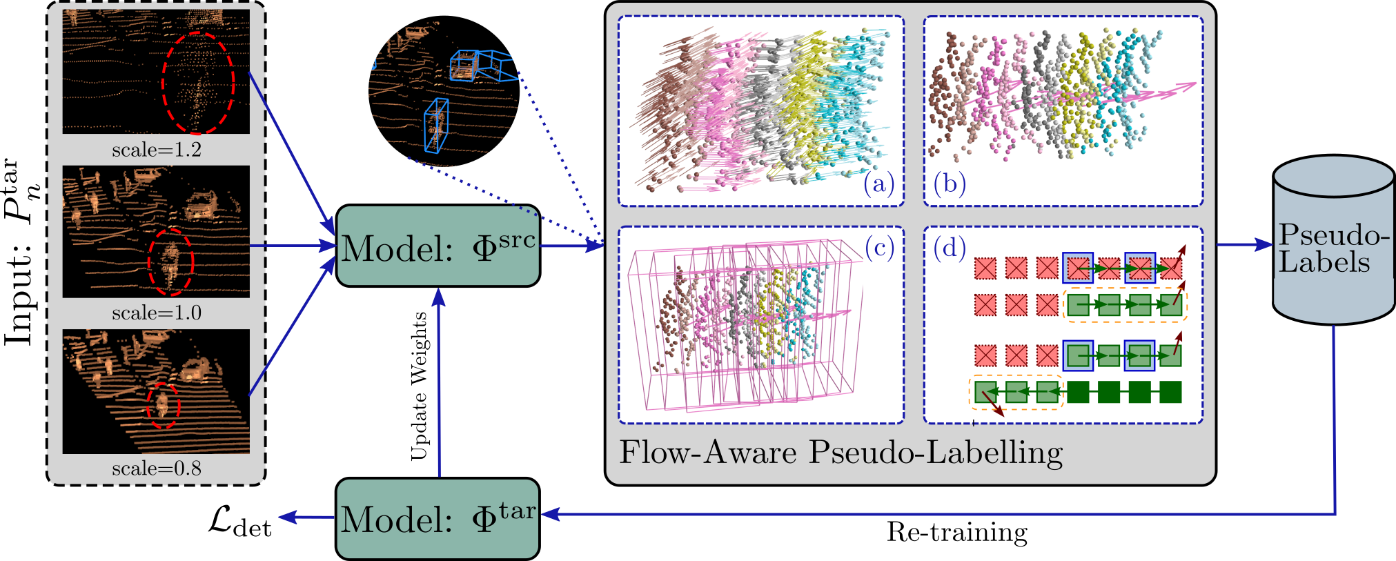
Figure 1: FAST3D scheme. The initial model $\Phi^{\text{src}}$, pre-trained on source data, generates non-confident detections on the target data for different scales. We leverage scene flow information (a) to calculate box flow (b), i.ethe mean flow of an object. This allows us to increase the recall and propagate labels through time (c). A final refinement step (d) reduces false positives and false negatives to obtain high-quality pseudo-labels for re-training. Points with the same colour originate from the same point cloud $P^{\text{tar}}_{n}$.

To overcome these issues, we present our Flow-Aware Self-Training approach for 3D object detection (FAST3D), leveraging scene flow [Liu et al.(2019a)Liu, Qi, and Guibas, Liu et al.(2019b)Liu, Yan, and Bohg, Wu et al.(2020)Wu, Wang, Li, Liu, and Fuxin] for robust pseudo-labels, as illustrated in Fig. 1. Scene flow estimates per-point correspondences between consecutive point clouds and calculates the motion vector for each point. Furthermore, although trained on synthetic data [Mayer et al.(2016)Mayer, Ilg, Häusser, Fischer, Cremers, Dosovitskiy, and Brox] only, scene flow estimators already achieve a favourable accuracy on real-world road data [Wu et al.(2020)Wu, Wang, Li, Liu, and Fuxin]. Thus, we investigate scene flow for UDA. In particular, we will show that scene flow allows us to propagate pseudo-labels reliably, recover missed objects and discard unreliable detections. This results in significantly improved pseudo-label quality which boosts the performance of self-training 3D detectors drastically.

We conduct experiments on the challenging Waymo Open Dataset (WOD) [Sun et al.(2020)Sun, Kretzschmar, Dotiwalla, Chouard, Patnaik, Tsui, Guo, Zhou, Chai, Caine, Vasudevan, Han, Ngiam, Zhao, Timofeev, Ettinger, Krivokon, Gao, Joshi, Zhang, Shlens, Chen, and Anguelov] considering two state-of-the-art 3D detectors, PointRCNN [Shi et al.(2019)Shi, Wang, and Li] and PV-RCNN [Shi et al.(2020a)Shi, Guo, Jiang, Wang, Shi, Wang, and Li], pre-trained on the much smaller KITTI dataset [Geiger et al.(2012)Geiger, Lenz, and Urtasun, Geiger et al.(2013)Geiger, Lenz, Stiller, and Urtasun]. Without any prior target domain knowledge (e.g [Wang et al.(2020a)Wang, Chen, You, Erran, Hariharan, Campbell, Weinberger, and Chao]), nor the need for source domain data (e.g [Yang et al.(2021)Yang, Shi, Wang, Li, and Qi]), we surpass the state-of-the-art by a significant margin.

2 Related Work

3D Object Detection

3D object detectors localize and classify an unknown number of objects within a 3D environment. Commonly, the identified objects are represented as tightly fitting oriented bounding boxes. Most recent 3D detectors, trained and evaluated on autonomous driving datasets, operate on LiDAR point clouds.

One way to categorize them is by their input representation. Voxel-based approaches [Lang et al.(2019)Lang, Vora, Caesar, Zhou, Yang, and Beijbom, Yan et al.(2018)Yan, Mao, and Li, Li(2017), Wang et al.(2020b)Wang, Fathi, Kundu, Ross, Pantofaru, Funkhouser, and Solomon, Yang et al.(2018)Yang, Luo, and Urtasun, Zhou and Tuzel(2018), Ye et al.(2020)Ye, Xu, and Cao, Deng et al.(2021)Deng, Shi, Li, Zhou, Zhang, and Li] rasterize the input space and assign points of irregular and sparse nature to grid cells of a fixed size. Afterwards, they either project these voxels directly to the bird’s eye view (BEV) or first learn feature representations by leveraging 3D convolutions and project them to BEV afterwards. Finally, a conventional 2D detection head predicts bounding boxes and class labels. Another line of work are point-based detectors [Ngiam et al.(2019)Ngiam, Caine, Han, Yang, Chai, Sun, Zhou, Yi, Alsharif, Nguyen, Chen, Shlens, and Vasudevan, Shi and Rajkumar(2020), Yang et al.(2020)Yang, Sun, Liu, and Jia, Shi et al.(2019)Shi, Wang, and Li]. In order to generate proposals directly from points, they leverage PointNet [Qi et al.(2017b)Qi, Su, Mo, and Guibas, Qi et al.(2017c)Qi, Yi, Su, and Guibas] to extract point-wise features. Hybrid approaches [Chen et al.(2019)Chen, Liu, Shen, and Jia, Shi et al.(2020b)Shi, Wang, Shi, Wang, and Li, Shi et al.(2020a)Shi, Guo, Jiang, Wang, Shi, Wang, and Li, He et al.(2020)He, Zeng, Huang, Hua, and Zhang, Yang et al.(2019)Yang, Sun, Liu, Shen, and Jia, Zhou et al.(2020)Zhou, Sun, Zhang, Anguelov, Gao, Ouyang, Guo, Ngiam, and Vasudevan], on the other hand, seek to leverage the advantages of both of the aforementioned strategies. In contrast to point cloud-only approaches, multi-modal detectors [Chen et al.(2017)Chen, Ma, Wan, Li, and Xia, Ku et al.(2018)Ku, Mozifian, Lee, Harakeh, and Waslander, Liang et al.(2019)Liang, Yang, Chen, Hu, and Urtasun, Liang et al.(2018)Liang, Yang, Wang, and Urtasun, Xu et al.(2018)Xu, Anguelov, and Jain, Qi et al.(2017a)Qi, Liu, Wu, Su, and Guibas] utilize 2D images complementary to LiDAR point clouds. The additional image information can be beneficial to recognise small objects.

Since most state-of-the-art approaches operate on LiDAR point clouds only, we also focus on this type of detectors. In particular, we demonstrate our self-training approach using PointRCNN [Shi et al.(2019)Shi, Wang, and Li] and PV-RCNN [Shi et al.(2020a)Shi, Guo, Jiang, Wang, Shi, Wang, and Li]. Both detectors have already been used in UDA settings for self-driving vehicles [Wang et al.(2020a)Wang, Chen, You, Erran, Hariharan, Campbell, Weinberger, and Chao, Yang et al.(2021)Yang, Shi, Wang, Li, and Qi] and achieve state-of-the-art robustness and accuracy.

Scene Flow

Scene flow represents the 3D motion field in the scene [Vedula et al.(2005)Vedula, Rander, Collins, and Kanade]. Recently, a relatively new area of research aims to estimate point-wise motion predictions in an end-to-end manner directly from raw point clouds [Liu et al.(2019a)Liu, Qi, and Guibas, Gu et al.(2019)Gu, Wang, Wu, Lee, and Wang, Wu et al.(2020)Wu, Wang, Li, Liu, and Fuxin]. With few exceptions [Liu et al.(2019b)Liu, Yan, and Bohg], most approaches process two consecutive point clouds as input. A huge benefit of data-driven scene flow models, especially regarding UDA, is their ability to learn in an unsupervised manner [Mittal et al.(2020)Mittal, Okorn, and Held, Wu et al.(2020)Wu, Wang, Li, Liu, and Fuxin, Li et al.(2021)Li, Lin, and Xie]. The biggest drawback of these networks is their huge memory consumption which limits the number of input points. To address this, [Jund et al.(2021)Jund, Sweeney, Abdo, Chen, and Shlens] proposes a light-weight model applicable to the dense Waymo Open Dataset [Sun et al.(2020)Sun, Kretzschmar, Dotiwalla, Chouard, Patnaik, Tsui, Guo, Zhou, Chai, Caine, Vasudevan, Han, Ngiam, Zhao, Timofeev, Ettinger, Krivokon, Gao, Joshi, Zhang, Shlens, Chen, and Anguelov] point clouds.

In our work, we use the 3D motion field to obtain robust and reliable pseudo-labels for UDA by leveraging the motion consistency of sequential detections. To this end, we utilize PointPWC [Wu et al.(2020)Wu, Wang, Li, Liu, and Fuxin] which achieves state-of-the-art scene flow estimation performance.

Unsupervised Domain Adaptation (UDA)

The common pipeline for UDA is to start with a model trained in a fully supervised manner on a label-rich source domain and adapt it on data from a label-scarce target domain in an unsupervised manner. Hence, the goal is to close the gap between both domains. There is already a large body of literature on UDA for 2D object detection in driving scenes [Chen et al.(2018)Chen, Li, Sakaridis, Dai, and Van Gool, He and Zhang(2019), Hsu et al.(2020)Hsu, Yao, Tsai, Hung, Tseng, Singh, and Yang, Kim et al.(2019)Kim, Jeong, Kim, Choi, and Kim, Rodriguez and Mikolajczyk(2019), Saito et al.(2019)Saito, Ushiku, Harada, and Saenko, Zhuang et al.(2020)Zhuang, Han, Huang, and Scott, Wang et al.(2019)Wang, Cai, Gao, and Vasconcelos, Xu et al.(2020)Xu, Zhao, Jin, and Wei]. Due to the growing number of publicly available large-scale autonomous driving datasets, UDA on 3D point cloud data has gained more interest recently [Qin et al.(2019)Qin, You, Wang, Kuo, and Fu, Jaritz et al.(2020)Jaritz, Vu, de Charette, Wirbel, and Pérez, Yi et al.(2020)Yi, Gong, and Funkhouser, Achituve et al.(2021)Achituve, Maron, and Chechik].

For LiDAR-based 3D object detection, [Wang et al.(2020a)Wang, Chen, You, Erran, Hariharan, Campbell, Weinberger, and Chao] demonstrate serious domain gaps between various datasets, mostly caused by different sensor setups (e.gresolution or mounting position) or geographic locations (e.gGermany $\to$ USA). A popular solution to UDA is self-training, as for the 2D case [Cai et al.(2019)Cai, Pan, Ngo, Tian, Duan, and Yao, Khodabandeh et al.(2019)Khodabandeh, Vahdat, Ranjbar, and Macready, RoyChowdhury et al.(2019)RoyChowdhury, Chakrabarty, Singh, Jin, Jiang, Cao, and Learned-Miller]. For example, [Yang et al.(2021)Yang, Shi, Wang, Li, and Qi] initially train the detector with random object scaling and an additional score prediction branch. Afterwards, pseudo-labels are updated in a cyclic manner considering previous examples. In order to overcome the need for source data, [Saltori et al.(2020)Saltori, Lathuiliére, Sebe, Ricci, and Galasso] performs test-time augmentation with multiple scales. The best matching labels are selected by checking motion coherency.

In contrast to [You et al.(2021)You, Diaz-Ruiz, Wang, Chao, Hariharan, Campbell, and Weinberger], where temporal information is exploited by probabilistic tracking, we propose to leverage scene flow. This enables us to reliably extract pseudo-labels despite initially low detection quality by exploiting motion consistency. As in [Saltori et al.(2020)Saltori, Lathuiliére, Sebe, Ricci, and Galasso], we also utilize test-time augmentation to overcome scaling issues, but we only need two additional scales.

3 Flow-Aware Self-Training

We now introduce our Flow-Aware Self-Training approach FAST3D, which consists of four steps as illustrated in Fig. 1. First, starting with a model trained on the source domain, we obtain initial 3D object detections for sequences of the target domain (Sec. 3.1). Second, we leverage scene flow to propagate these detections throughout the sequences and obtain tracks, robust to the initial detection quality (Sec. 3.2). Third, we recover potentially missed tracks and correct false positives in a refinement step (Sec. 3.3). Finally, we extract pseudo-labels for self-training to improve the initial model (Sec. 3.4).

Problem Statement

Given a 3D object detection model $\Phi^{\text{src}}$ pre-trained on $N^{\text{src}}$ source domain frames $\{(P^{\text{src}}_{n},L^{\text{src}}_{n})\}_{n=1}^{N^{\text{src}}}$, our task is to adapt to unseen target data with $N^{\text{tar}}$ unlabelled sequences $\{S^{\text{tar}}_{i}\}_{i=1}^{N^{\text{tar}}}$, where $S^{\text{tar}}_{i}=\{P^{\text{tar}}_{n}\}_{n=1}^{N_{i}^{\text{tar}}}$ with varying length $N_{i}^{\text{tar}}$. Here, $P_{n}$ and $L_{n}$ denote the point cloud and corresponding labels of the $n^{\text{th}}$ frame. To obtain the target detection model $\Phi^{\text{tar}}$, we apply self-training which assumes that both domains contain the same set of classes (i.evehicle/car, pedestrian, cyclist) but these are drawn from different distributions. In the following, we show how to self-train a detection model $\Phi^{\text{tar}}$ without access to source data or target label statistics (as e.g [Wang et al.(2020a)Wang, Chen, You, Erran, Hariharan, Campbell, Weinberger, and Chao]) and without modifying the source model in any way (as e.g [Yang et al.(2021)Yang, Shi, Wang, Li, and Qi]) to achieve performance beyond the state-of-the-art. Because we only work with target domain data, we omit the domain superscripts to improve readability.

3.1 Pseudo-Label Generation

The first step, as in all self-training approaches (e.g [Yang et al.(2021)Yang, Shi, Wang, Li, and Qi, You et al.(2021)You, Diaz-Ruiz, Wang, Chao, Hariharan, Campbell, and Weinberger, Saltori et al.(2020)Saltori, Lathuiliére, Sebe, Ricci, and Galasso]), is to run the initial source model $\Phi^{\text{src}}$ on the target data and keep high-confident detections. More formally, the $j^{\text{th}}$ detection at frame $n$ is represented by its bounding box $\mathbf{b}_{j,n}=\left(\mathbf{p},\mathbf{d},\theta\right)$ and confidence score $c_{j,n}^{\mathbf{b}}$. Each box is defined by its centre position $\mathbf{p}=(c_{x},c_{y},c_{z})$, dimension $\mathbf{d}=(l,w,h)$ and heading angle $\theta$. Note that we can use any vanilla 3D object detector, since we do not change the initial model at all, not even by adapting the mean object size of anchors (as in [Yang et al.(2021)Yang, Shi, Wang, Li, and Qi]). In order to deal with different object sizes between various datasets without pre-training $\Phi^{\text{src}}$ on scaled source data [Yang et al.(2021)Yang, Shi, Wang, Li, and Qi, Wang et al.(2020a)Wang, Chen, You, Erran, Hariharan, Campbell, Weinberger, and Chao], we leverage test-time augmentation instead. In particular, we feed $\Phi^{\text{src}}$ with three scales (i.e 0.8, 1.0, 1.2) of the same point cloud, similar to [Saltori et al.(2020)Saltori, Lathuiliére, Sebe, Ricci, and Galasso]. However, [Saltori et al.(2020)Saltori, Lathuiliére, Sebe, Ricci, and Galasso] requires to run the detector on 125 different scale levels (due to different scaling factors along each axis). By leveraging scene flow, we only need three scales to robustly handle both larger and smaller objects. We combine the detection outputs at all three scales via non-maximum suppression (NMS) and threshold the detections at a confidence of $c_{j,n}^{\mathbf{b}}\geq 0.8$ to obtain the initial high-confident detections.

3.2 Flow-Aware Pseudo-Label Propagation

Keeping only high-confident detections of the source model gets rid of false positives (FP) but also results in a lot of false negatives (FN). While this can partially be addressed via multi-target tracking (MTT), e.g [You et al.(2021)You, Diaz-Ruiz, Wang, Chao, Hariharan, Campbell, and Weinberger], standard MTT approaches (such as [Weng et al.(2020)Weng, Wang, Held, and Kitani]) are not suitable for low quality detections because of their hand-crafted motion prediction. Due to the domain gap, however, the detection quality of the source model will inevitably be low.

To overcome this issue, we introduce our scene flow-aware tracker. We define a set of tracks $T=\{t_{1},t_{2},\dots,t_{k}\}$ where each track $t_{k}$ contains a list of bounding boxes and is represented by its current state $\mathbf{x}_{k,n}$, i.eits bounding box, and track confidence score $c_{k,n}^{\mathbf{t}}$. Following the tracking-by-detection paradigm, we use the high-confident detections and match them in subsequent frames. Instead of hand-crafted motion models, however, we utilize scene flow to propagate detections. More formally, given two consecutive point clouds $P_{n-1}$ and $P_{n}$, PointPWC [Wu et al.(2020)Wu, Wang, Li, Liu, and Fuxin] estimates the motion vector $\mathbf{v}_{i,n-1}=(v_{x},v_{y},v_{z})_{i,n-1}$ for each point $\mathbf{p}_{i,n-1}\in P_{n-1}$. We then average all motion vectors within a track’s bounding box $\mathbf{x}_{k,n-1}$ to compute its mean flow $\mathbf{v}_{k,n-1}$. To get the predicted state $\mathbf{x}_{k,n|n-1}$ for the current frame $n$, we estimate the position of each track as $\mathbf{p}_{k,n|n-1}=\mathbf{p}_{k,n-1}+\mathbf{v}_{k,n-1}$. We then assign detections to tracks via the Hungarian algorithm [Kuhn and Yaw(1955)], where we use the intersection over union between the detections $\mathbf{b}_{j,n}$ and the predicted tracks $\mathbf{x}_{k,n|n-1}$.

We initialize a new track for each unassigned detection. This naive initialisation ensures that we include all object tracks, whereas potentially wrong tracks can easily be filtered in our refinement step (Sec. 3.3). Initially, we set a track’s confidence $c_{k,n}^{\mathbf{t}}$ to the detection confidence $c_{j,n}^{\mathbf{b}}$. For each assigned pair, we perform a weighted update based on the confidence scores as $\mathbf{x}_{k,n|n}=\frac{c_{k,n-1}^{\mathbf{t}}\mathbf{x}_{k,n|n-1}+c_{j,n}^{\mathbf{b}}\mathbf{b}_{j,n}}{c_{k,n-1}^{\mathbf{t}}+c_{j,n}^{\mathbf{b}}}$ and update the track confidence $c_{k,n}^{\mathbf{t}}=\frac{(c_{k,n-1}^{\mathbf{t}})^{2}+(c_{j,n}^{\mathbf{b}})^{2}}{c_{k,n-1}^{\mathbf{t}}+c_{j,n}^{\mathbf{b}}}$. Note that we update the track’s heading angle only if the orientation change is less than $30^{\circ}$, otherwise we keep its previous orientation. For boxes with only very few point correspondences, the flow estimates may be noisy. To suppress such flow outliers, we allow a maximum change in velocity of $1.5~{}\text{m/s}$, along with the maximum orientation change of $30^{\circ}$. If the estimated flow exceeds these limits, we keep the previous estimate.

For track termination, we distinguish moving (i.e$\mathbf{v}_{k,n-1}>0.8~{}\text{m/s}$) and static objects. For moving objects, we terminate their tracks if there are no more points within their bounding box. Static object tracks are kept alive as long as they are within the field-of-view. This ensures that even long term occlusions can be handled, as such objects will eventually contain points or be removed during refinement.

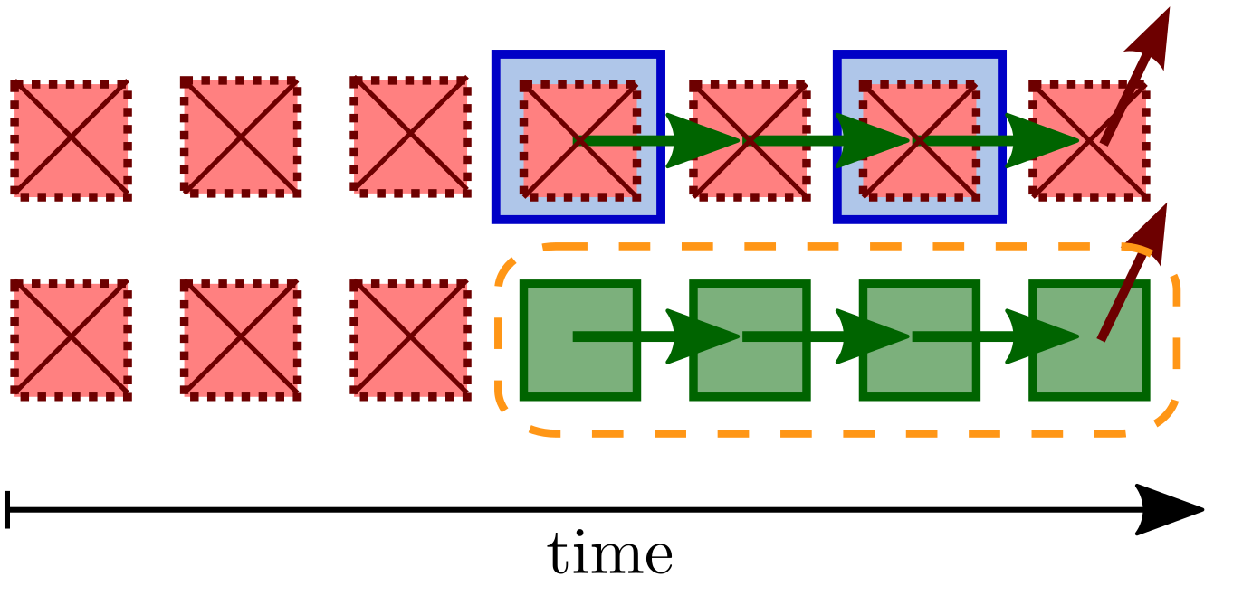
(a) Recovery via flow consistency.

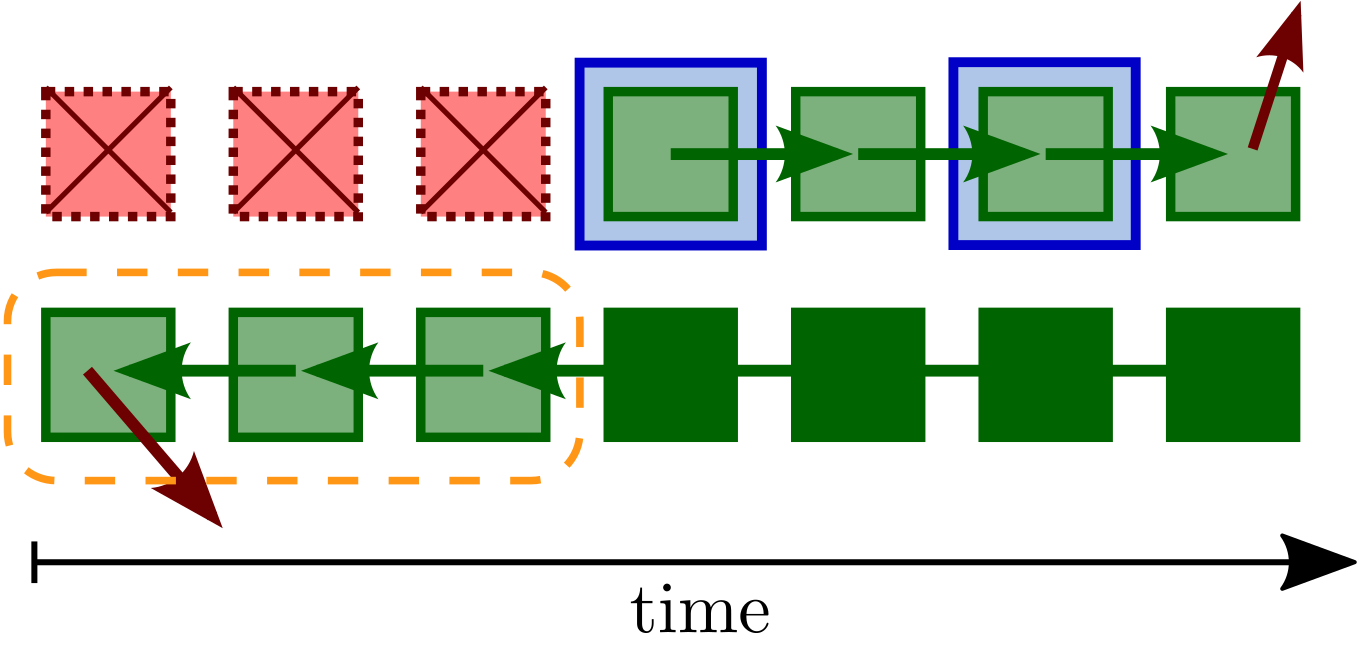
(b) Backward tracking.

Figure 2: Track refinement to address the initially low detection quality on the target domain. The valid track, false negative (missed) and true positive detections are illustrated in green, red and blue, respectively. Green and red arrows show valid and inconsistent flow (high change in orientation/velocity), respectively. (a) Flow consistency recovers object tracks with low detection hit ratio. (b) Starting from the first detection, backward tracking propagates the bounding box back in time to recover missing tails. Refined tracks are marked by the dashed orange regions.

3.3 Pseudo-Label Refinement

Due to our simplified track management (initialisation and termination), we now have tracks covering most of the visible objects but suffer from several false positive tracks. However, these can easily be corrected in the following refinement step.

Track Filtering and Correction

We first compute the hit ratio for each track, i.ethe number of assigned detections divided by the track’s length. Tracks are removed if their hit ratio is less than $0.3$. Additionally, we discard tracks shorter than $0.5~{}\text{s}$ (i.e5 frames at the typical LiDAR frequency of $10~{}\text{Hz}$) and tracks which detections never exceed 15 points (to suppress spurious detections).

In our experiments, we observed that detections are most accurate on objects with more points (as opposed to the confidence score which is usually less reliable due to the domain gap). Thus, we sort a track’s assigned detections by the number of contained points and compute the average dimension over the top three. We then apply this average dimension to all boxes of the track. Additionally, for static cars we also apply the average position and heading angle to all boxes of the track since these properties cannot change for rigid static objects.

Track Recovery

This conservative filtering of unreliable tracks ensures a lower number of false positives. However, true positive tracks with only very few detections might be removed prematurely. In order to recover these, we leverage flow consistency. As illustrated in Fig. 2(a), we consider removed tracks with at least two non-overlapping detections (i.emoving objects). For these tracks, we propagate the first detection by solely utilizing the scene flow estimates. If this flow-extrapolated box overlaps with the other detections (minimum IoU of $0.3$), we recover this track.

Backward Completion

A common drawback of the tracking-by-detection paradigm is late initialization caused by missing detections at the beginning of the track. To overcome this issue, we look backwards for each track as illustrated in Fig. 2(b) to extend missing tails. Hence, we leverage scene flow in the opposite direction and propagate the bounding box back in time. We propagate backwards as long as the flow is consistent, meaning no unreasonable changes in velocity or direction, and the predicted box location contains points. To avoid including the ground plane in the latter condition, we count only points within the upper $70\,\%$ of the bounding box volume.

3.4 Self-Training

We use the individual bounding boxes of the refined tracks as high-quality pseudo-labels to re-train the detection model. To this end, we use standard augmentation strategies, i.e randomized world scaling, flipping, rotation, as well as ground truth sampling [Shi et al.(2020a)Shi, Guo, Jiang, Wang, Shi, Wang, and Li, Yan et al.(2018)Yan, Mao, and Li]. As we don’t need to modify the initial model $\Phi^{\text{src}}$, we also use its detection loss $\mathcal{L}_{\text{det}}$ without modifications for re-training.

4 Experiments

In the following, we present the results of our flow-aware self-training approach using two vanilla 3D object detectors. Additional evaluations demonstrating the improved pseudo-label quality are included in the supplemental material.

4.1 Datasets and Evaluation Details

Datasets

We conduct experiments on the challenging Waymo Open Dataset (WOD) [Sun et al.(2020)Sun, Kretzschmar, Dotiwalla, Chouard, Patnaik, Tsui, Guo, Zhou, Chai, Caine, Vasudevan, Han, Ngiam, Zhao, Timofeev, Ettinger, Krivokon, Gao, Joshi, Zhang, Shlens, Chen, and Anguelov] with a source model $\Phi^{s}$ pre-trained on the KITTI dataset [Geiger et al.(2012)Geiger, Lenz, and Urtasun, Geiger et al.(2013)Geiger, Lenz, Stiller, and Urtasun]. We sample 200 sequences ($\sim$25%) from the WOD training set for pseudo-label generation and 20 sequences ($\sim$10%) from the WOD validation set for testing. With this evaluation, we cover various sources of domain shifts: geographic location (Germany $\rightarrow$ USA), sensor setup (Velodyne $\rightarrow$ Waymo LiDAR) and weather (broad daylight $\rightarrow$ sunny, rain, night). In contrast to recent work, we do not only consider the car/vehicle class, but also pedestrians and cyclists. Because the initial model $\Phi^{s}$ is trained on front view scans only (available KITTI annotations), we stick to this setup for evaluation.

Evaluation Metrics

We follow the official WOD evaluation protocol [Sun et al.(2020)Sun, Kretzschmar, Dotiwalla, Chouard, Patnaik, Tsui, Guo, Zhou, Chai, Caine, Vasudevan, Han, Ngiam, Zhao, Timofeev, Ettinger, Krivokon, Gao, Joshi, Zhang, Shlens, Chen, and Anguelov] and report the average precision (AP) for the intersection over union (IoU) thresholds $0.7$ and $0.5$ for vehicles, as well as $0.5$ and $0.25$ for pedestrians and cyclists. AP is reported for both bird’s eye view (BEV) and 3D – denoted as $\text{AP}_{\text{BEV}}$ and $\text{AP}_{\text{3D}}$ – for different ranges: $0\,\text{m}-30\,\text{m}$, $30\,\text{m}-50\,\text{m}$ and $50\,\text{m}-75\,\text{m}$. Additionally, we calculate the closed gap as in [Yang et al.(2021)Yang, Shi, Wang, Li, and Qi].

Comparisons

The lower performance bound is to directly apply the source model $\Phi^{s}$ on the target data, denoted source only (SO). The fully supervised model (FS) trained on the whole target data ($\sim 25\%$ of WOD) on the other hand defines the upper performance bound. Statistical normalization (SN) [Wang et al.(2020a)Wang, Chen, You, Erran, Hariharan, Campbell, Weinberger, and Chao] is the state-of-the-art on UDA for 3D object detection and leverages target data statistics. The recent DREAMING [You et al.(2021)You, Diaz-Ruiz, Wang, Chao, Hariharan, Campbell, and Weinberger] approach also exploits temporal information for UDA. Finally, we also compare against the few shot [Wang et al.(2020a)Wang, Chen, You, Erran, Hariharan, Campbell, Weinberger, and Chao] approach which adapts the model using a few fully labelled sequences of the target domain.

Implementation details

We demonstrate FAST3D with two detectors, PointRCNN [Shi et al.(2019)Shi, Wang, and Li] and PV-RCNN [Shi et al.(2020a)Shi, Guo, Jiang, Wang, Shi, Wang, and Li] from OpenPCDet [Team(2020)], configured as in their official implementations. To compensate for the ego-vehicle motion, we project all frames of a sequence into the world coordinate system by computing the ego-vehicle poses [Sun et al.(2020)Sun, Kretzschmar, Dotiwalla, Chouard, Patnaik, Tsui, Guo, Zhou, Chai, Caine, Vasudevan, Han, Ngiam, Zhao, Timofeev, Ettinger, Krivokon, Gao, Joshi, Zhang, Shlens, Chen, and Anguelov]. We slightly increase the field-of-view (FOV) from approximately $45^{\circ}$ to $60^{\circ}$, which simplifies handling pseudo-label tracks at the edge of the narrower FOV. In each self-training cycle, we re-train the detector for $4$ epochs with Adam [Kingma and Ba(2015)] and a learning rate of $3\times 10^{-4}$ until we reach convergence (i.ePointRCNN 2 cycles, PV-RCNN 3 cycles).

We estimate the scene flow using PointPWC [Wu et al.(2020)Wu, Wang, Li, Liu, and Fuxin]. Although PointPWC, similar to other flow estimators [Li et al.(2021)Li, Lin, and Xie, Mittal et al.(2020)Mittal, Okorn, and Held], could be fine-tuned in a self-supervised fashion, we use the off-the-shelf model pre-trained only on synthetic data [Mayer et al.(2016)Mayer, Ilg, Häusser, Fischer, Cremers, Dosovitskiy, and Brox]. This allows us to demonstrate the benefits and simplicity of leveraging 3D motion without additional fine-tuning. To prepare the point clouds for scene flow estimation, we use RANSAC [Fischler and Bolles(1981)] to remove ground points (as in [Wu et al.(2020)Wu, Wang, Li, Liu, and Fuxin]) and randomly subsample the larger input point cloud to match the smaller one.

4.2 Empirical Results

In Table 1 we compare FAST3D for two detectors with the source only (SO) and fully supervised (FS) strategies, which define the lower and upper performance bound, respectively. Across all classes and different IoU thresholds, we manage to close the domain gap significantly (36% to 87%), achieving almost the fully supervised oracle performance although our approach is unsupervised and does not rely on any prior knowledge about the target domain. To the best of our knowledge, we are the first to additionally report adaptation performance for both pedestrians and cyclists as these vulnerable road users should not be neglected in evaluations. We focus this evaluation on $\text{AP}_{\text{3D}}$ because (in contrast to $\text{AP}_{\text{BEV}}$) this metric also penalizes estimation errors along the $z$-axis (i.evertical centre and height). Consequently, $\text{AP}_{\text{BEV}}$ scores are usually much higher than $\text{AP}_{\text{3D}}$.

Since reporting the closed domain gap has only been proposed very recently [Yang et al.(2021)Yang, Shi, Wang, Li, and Qi], no other approaches reported this closure for KITTI$\rightarrow$WOD yet. We can, however, relate the results for the most similar setting, i.eadaptation of PV-RCNN for the car/vehicle class, where we achieve a closed gap of 76.5% (KITTI$\rightarrow$WOD, vehicles within all sensing ranges) in contrast to 70.7% of [Yang et al.(2021)Yang, Shi, Wang, Li, and Qi] (WOD$\rightarrow$KITTI, cars within KITTI’s moderate difficulty). Despite the different settings, we achieve a favourable domain gap closure while evaluating on the more challenging KITTI$\rightarrow$WOD. In particular, according to [Wang et al.(2020a)Wang, Chen, You, Erran, Hariharan, Campbell, Weinberger, and Chao], starting from KITTI as the source domain is the most difficult setting for UDA, as it has orders of magnitude fewer samples than other datasets. Additionally, KITTI contains only sunny daylight data and its car class does not include trucks, vans or buses which are, however, contained in the WOD vehicle class.

		Class	PointRCNN				PV-RCNN
			SO	FAST3D	FS	Closed Gap	SO	FAST3D	FS	Closed Gap
AP3D	0.7	Vehicle	08.0	58.1	65.6	87.0 %	10.3	63.6	80.0	76.5 %
	0.5	Pedestrian	18.9	36.8	47.8	62.0 %	13.7	44.7	74.4	51.1 %
	0.5	Cyclist	24.2	48.0	60.0	66.5 %	14.6	35.6	72.9	36.0 %
AP3D	0.5	Vehicle	60.0	77.3	80.9	82.8 %	50.3	85.1	95.2	77.5 %
	0.25	Pedestrian	30.8	41.7	52.2	50.9 %	21.6	57.2	85.4	55.8 %
	0.25	Cyclist	31.8	66.2	69.0	92.5 %	32.5	49.4	75.5	39.3 %

Table 1: Our FAST3D compared to lower (source-only, SO) and upper (fully-supervised, FS) bound, on KITTI $\rightarrow$ Waymo Open Dataset (WOD) for different IoU thresholds.

Table 2 reports the results in $\text{AP}_{\text{3D}}$ split by their detection range for different intersection over union (IoU) thresholds. We can observe that our self-training pipeline significantly improves the initial model on all ranges. The only notable outlier are cyclists within the far range of 50–75 meters, where even after re-training both detectors achieve rather low scores. This is due to the low number of far range cyclists within the WOD validation set, i.eonly a few detection failures already drastically degrade the $\text{AP}_{\text{3D}}$ for the cyclist class.

		Class	PointRCNN			PV-RCNN
			0m - 30m	30m - 50m	50m - 75m	0m - 30m	30m - 50m	50m - 75m
AP3D	0.7	Vehicle	70.3	58.7	37.0	74.9	64.6	44.0
	0.5	Pedestrian	66.2	45.7	14.6	66.5	55.0	22.7
	0.5	Cyclist	76.7	65.7	04.9	64.4	46.0	01.4
AP3D	0.5	Vehicle	86.9	79.3	63.5	91.2	85.9	70.4
	0.25	Pedestrian	74.1	50.3	17.4	78.0	67.3	36.4
	0.25	Cyclist	93.9	76.2	33.6	90.6	54.4	05.0

Table 2: Detailed results at different sensing ranges (KITTI $\rightarrow$ WOD) for two detectors at different IoU thresholds.

4.3 Comparison with the State-of-the-Art

To fairly compare with the state-of-the-art in Table 3, we follow the common protocol and report both $\text{AP}_{\text{3D}}$ and $\text{AP}_{\text{BEV}}$ on the vehicle class. We clearly outperform the best approach (statistical normalization), even though this method utilizes target data statistics and is thus considered weakly supervised, whereas our approach is unsupervised. We also outperform the only temporal 3D pseudo-label approach [You et al.(2021)You, Diaz-Ruiz, Wang, Chao, Hariharan, Campbell, and Weinberger] by a huge margin for all ranges, especially at the high-quality $\text{IoU}\geq 0.7$. Moreover, we perform on par with the few shot approach from [Wang et al.(2020a)Wang, Chen, You, Erran, Hariharan, Campbell, Weinberger, and Chao] on close-range data and even outperform it on medium and far ranges.

Method	IoU 0.7			IoU 0.5
	0m - 30m	30m - 50m	50m - 75m	0m - 30m	30m - 50m	50m - 75m
SO	29.2 / 10.0	27.2 /  8.0	24.7 /  4.2	67.8 / 66.8	70.2 / 63.9	48.0 / 38.5
SN [Wang et al.(2020a)Wang, Chen, You, Erran, Hariharan, Campbell, Weinberger, and Chao]	87.1 / 60.1	78.1 / 54.9	46.8 / 25.1	-	-	-
DREAMING [You et al.(2021)You, Diaz-Ruiz, Wang, Chao, Hariharan, Campbell, and Weinberger]	51.4 / 13.8	44.5 / 16.7	25.6 /  7.8	81.1 / 78.5	69.9 / 61.8	50.2 / 41.0
FAST3D (ours)	81.7 / 70.3	75.4 / 58.7	52.4 / 37.0	87.2 / 74.9	81.2 / 64.6	68.6 / 44.0
Few Shot [Wang et al.(2020a)Wang, Chen, You, Erran, Hariharan, Campbell, Weinberger, and Chao]	88.7 / 74.1	78.1 / 57.2	45.2 / 24.3	-	-	-
FS	86.2 / 78.5	77.8 / 63.7	60.8 / 48.1	91.7 / 92.1	83.7 / 78.3	73.3 / 69.7

Table 3: Comparison to the state-of-the-art for KITTI $\rightarrow$ WOD. All approaches adapt PointRCNN. Following the common protocol, results are listed for the vehicle class at different sensing ranges reported in $\text{AP}_{\text{BEV}}$ / $\text{AP}_{\text{3D}}$.

5 Conclusion

We presented a flow-aware self-training pipeline for unsupervised domain adaptation of 3D object detectors on sequential LiDAR point clouds. Leveraging motion consistency via scene flow, we obtain reliable and precise pseudo-labels at high recall levels. We do not exploit any prior target domain knowledge, nor do we need to modify the 3D detector in any way. As demonstrated in our evaluations, we surpass the current state-of-the-art in self-training for UDA by a large margin.

References

- [Achituve et al.(2021)Achituve, Maron, and Chechik] Idan Achituve, Haggai Maron, and Gal Chechik. Self-Supervised Learning for Domain Adaptation on Point Clouds. In Proc. WACV, 2021.
- [Caesar et al.(2020)Caesar, Bankiti, Lang, Vora, Liong, Xu, Krishnan, Pan, Baldan, and Beijbom] Holger Caesar, Varun Bankiti, Alex H. Lang, Sourabh Vora, Venice Erin Liong, Qiang Xu, Anush Krishnan, Yu Pan, Giancarlo Baldan, and Oscar Beijbom. nuScenes: A Multimodal Dataset for Autonomous Driving. In Proc. CVPR, 2020.
- [Cai et al.(2019)Cai, Pan, Ngo, Tian, Duan, and Yao] Qi Cai, Yingwei Pan, Chong-Wah Ngo, Xinmei Tian, Lingyu Duan, and Ting Yao. Exploring Object Relation in Mean Teacher for Cross-Domain Detection. In Proc. CVPR, 2019.
- [Chen et al.(2017)Chen, Ma, Wan, Li, and Xia] Xiaozhi Chen, Huimin Ma, Ji Wan, Bo Li, and Tian Xia. Multi-view 3D Object Detection Network for Autonomous Driving. In Proc. CVPR, 2017.
- [Chen et al.(2019)Chen, Liu, Shen, and Jia] Yilun Chen, Shu Liu, Xiaoyong Shen, and Jiaya Jia. Fast Point R-CNN. In Proc. ICCV, 2019.
- [Chen et al.(2018)Chen, Li, Sakaridis, Dai, and Van Gool] Yuhua Chen, Wen Li, Christos Sakaridis, Dengxin Dai, and Luc Van Gool. Domain Adaptive Faster R-CNN for Object Detection in the Wild. In Proc. CVPR, 2018.
- [Deng et al.(2021)Deng, Shi, Li, Zhou, Zhang, and Li] Jiajun Deng, Shaoshuai Shi, Peiwei Li, Wengang Zhou, Yanyong Zhang, and Houqiang Li. Voxel R-CNN: Towards High Performance Voxel-based 3D Object Detection. In Proc. AAAI, 2021.
- [Fischler and Bolles(1981)] Martin A. Fischler and Robert C. Bolles. Random Sample Consensus: A Paradigm for Model Fitting with Applications to Image Analysis and Automated Cartography. Commun. ACM, 24(6):381–395, 1981.
- [Geiger et al.(2012)Geiger, Lenz, and Urtasun] Andreas Geiger, Philip Lenz, and Raquel Urtasun. Are we ready for Autonomous Driving? The KITTI Vision Benchmark Suite. In Proc. CVPR, 2012.
- [Geiger et al.(2013)Geiger, Lenz, Stiller, and Urtasun] Andreas Geiger, Philip Lenz, Christoph Stiller, and Raquel Urtasun. Vision meets Robotics: The KITTI Dataset. IJRR, 2013.
- [Gu et al.(2019)Gu, Wang, Wu, Lee, and Wang] Xiuye Gu, Yijie Wang, Chongruo Wu, Yong Jae Lee, and Panqu Wang. HPLFlowNet: Hierarchical Permutohedral Lattice FlowNet for Scene Flow Estimation on Large-Scale Point Clouds. In Proc. CVPR, 2019.
- [He et al.(2020)He, Zeng, Huang, Hua, and Zhang] Chenhang He, Hui Zeng, Jianqiang Huang, Xian-Sheng Hua, and Lei Zhang. Structure Aware Single-stage 3D Object Detection from Point Cloud. In Proc. CVPR, 2020.
- [He and Zhang(2019)] Zhenwei He and Lei Zhang. Multi-Adversarial Faster-RCNN for Unrestricted Object Detection. In Proc. ICCV, 2019.
- [Hsu et al.(2020)Hsu, Yao, Tsai, Hung, Tseng, Singh, and Yang] Han-Kai Hsu, Chun-Han Yao, Yi-Hsuan Tsai, Wei-Chih Hung, Hung-Yu Tseng, Maneesh Singh, and Ming-Hsuan Yang. Progressive Domain Adaptation for Object Detection. In Proc. WACV, 2020.
- [Jaritz et al.(2020)Jaritz, Vu, de Charette, Wirbel, and Pérez] Maximilian Jaritz, Tuan-Hung Vu, Raoul de Charette, Emilie Wirbel, and Patrick Pérez. xMUDA: Cross-modal unsupervised domain adaptation for 3D semantic segmentation. In Proc. CVPR, 2020.
- [Jund et al.(2021)Jund, Sweeney, Abdo, Chen, and Shlens] Philipp Jund, Chris Sweeney, Nichola Abdo, Zhifeng Chen, and Jonathon Shlens. Scalable Scene Flow from Point Clouds in the Real World. arXiv CoRR, abs/2103.01306, 2021.
- [Khodabandeh et al.(2019)Khodabandeh, Vahdat, Ranjbar, and Macready] Mehran Khodabandeh, Arash Vahdat, Mani Ranjbar, and William G. Macready. A Robust Learning Approach to Domain Adaptive Object Detection. In Proc. ICCV, 2019.
- [Kim et al.(2019)Kim, Jeong, Kim, Choi, and Kim] Taekyung Kim, Minki Jeong, Seunghyeon Kim, Seokeon Choi, and Changick Kim. Diversify and Match: A Domain Adaptive Representation Learning Paradigm for Object Detection. In Proc. CVPR, 2019.
- [Kingma and Ba(2015)] Diederik P. Kingma and Jimmy Ba. Adam: A Method for Stochastic Optimization. In Proc. ICLR, 2015.
- [Ku et al.(2018)Ku, Mozifian, Lee, Harakeh, and Waslander] Jason Ku, Melissa Mozifian, Jungwook Lee, Ali Harakeh, and Steven Waslander. Joint 3D Proposal Generation and Object Detection from View Aggregation. In Proc. IROS, 2018.
- [Kuhn and Yaw(1955)] H. W. Kuhn and Bryn Yaw. The Hungarian method for the assignment problem. Naval Res. Logist. Quart, pages 83–97, 1955.
- [Lang et al.(2019)Lang, Vora, Caesar, Zhou, Yang, and Beijbom] Alex H Lang, Sourabh Vora, Holger Caesar, Lubing Zhou, Jiong Yang, and Oscar Beijbom. Pointpillars: Fast encoders for object detection from point clouds. In Proc. CVPR, 2019.
- [Li(2017)] Bo Li. 3D fully convolutional network for vehicle detection in point cloud. In Proc. IROS, 2017.
- [Li et al.(2021)Li, Lin, and Xie] Ruibo Li, Guosheng Lin, and Lihua Xie. Self-Point-Flow: Self-Supervised Scene Flow Estimation from Point Clouds with Optimal Transport and Random Walk. In Proc. CVPR, 2021.
- [Liang et al.(2018)Liang, Yang, Wang, and Urtasun] Ming Liang, Bin Yang, Shenlong Wang, and Raquel Urtasun. Deep Continuous Fusion for Multi-Sensor 3D Object Detection. In Proc. ECCV, 2018.
- [Liang et al.(2019)Liang, Yang, Chen, Hu, and Urtasun] Ming Liang, Bin Yang, Yun Chen, Rui Hu, and Raquel Urtasun. Multi-Task Multi-Sensor Fusion for 3D Object Detection. In Proc. CVPR, 2019.
- [Liu et al.(2019a)Liu, Qi, and Guibas] Xingyu Liu, Charles R Qi, and Leonidas J Guibas. FlowNet3D: Learning Scene Flow in 3D Point Clouds. In Proc. CVPR, 2019a.
- [Liu et al.(2019b)Liu, Yan, and Bohg] Xingyu Liu, Mengyuan Yan, and Jeannette Bohg. MeteorNet: Deep Learning on Dynamic 3D Point Cloud Sequences. In Proc. ICCV, 2019b.
- [Mayer et al.(2016)Mayer, Ilg, Häusser, Fischer, Cremers, Dosovitskiy, and Brox] N. Mayer, E. Ilg, P. Häusser, P. Fischer, D. Cremers, A. Dosovitskiy, and T. Brox. A Large Dataset to Train Convolutional Networks for Disparity, Optical Flow, and Scene Flow Estimation. In Proc. CVPR, 2016.
- [Meng et al.(2020)Meng, Wang, Zhou, Shen, Van Gool, and Dai] Qinghao Meng, Wenguan Wang, Tianfei Zhou, Jianbing Shen, Luc Van Gool, and Dengxin Dai. Weakly Supervised 3D Object Detection from Lidar Point Cloud. In Proc. ECCV, 2020.
- [Mittal et al.(2020)Mittal, Okorn, and Held] Himangi Mittal, Brian Okorn, and David Held. Just Go With the Flow: Self-Supervised Scene Flow Estimation. In Proc. CVPR, 2020.
- [Ngiam et al.(2019)Ngiam, Caine, Han, Yang, Chai, Sun, Zhou, Yi, Alsharif, Nguyen, Chen, Shlens, and Vasudevan] Jiquan Ngiam, Benjamin Caine, Wei Han, Brandon Yang, Yuning Chai, Pei Sun, Yin Zhou, Xi Yi, Ouais Alsharif, Patrick Nguyen, Zhifeng Chen, Jonathon Shlens, and Vijay Vasudevan. StarNet: Targeted Computation for Object Detection in Point Clouds. arXiv CoRR, abs/1908.11069, 2019.
- [Qi et al.(2017a)Qi, Liu, Wu, Su, and Guibas] Charles R Qi, Wei Liu, Chenxia Wu, Hao Su, and Leonidas J Guibas. Frustum PointNets for 3D Object Detection from RGB-D Data. In Proc. CVPR, 2017a.
- [Qi et al.(2017b)Qi, Su, Mo, and Guibas] Charles R Qi, Hao Su, Kaichun Mo, and Leonidas J. Guibas. PointNet: Deep Learning on Point Sets for 3D Classification and Segmentation. In Proc. CVPR, 2017b.
- [Qi et al.(2017c)Qi, Yi, Su, and Guibas] Charles R. Qi, Li Yi, Hao Su, and Leonidas J. Guibas. PointNet++: Deep Hierarchical Feature Learning on Point Sets in a Metric Space. In Proc. NeurIPS, 2017c.
- [Qin et al.(2019)Qin, You, Wang, Kuo, and Fu] Can Qin, Haoxuan You, L. Wang, C.-C. Jay Kuo, and Yun Fu. PointDAN: A Multi-Scale 3D Domain Adaption Network for Point Cloud Representation. In Proc. NeurIPS, 2019.
- [Rodriguez and Mikolajczyk(2019)] A. L. Rodriguez and K. Mikolajczyk. Domain Adaptation for Object Detection via Style Consistency. In Proc. BMVC, 2019.
- [RoyChowdhury et al.(2019)RoyChowdhury, Chakrabarty, Singh, Jin, Jiang, Cao, and Learned-Miller] Aruni RoyChowdhury, Prithvijit Chakrabarty, Ashish Singh, SouYoung Jin, Huaizu Jiang, Liangliang Cao, and Erik Learned-Miller. Automatic Adaptation of Object Detectors to New Domains Using Self-Training. In Proc. CVPR, 2019.
- [Saito et al.(2019)Saito, Ushiku, Harada, and Saenko] Kuniaki Saito, Yoshitaka Ushiku, Tatsuya Harada, and Kate Saenko. Strong-Weak Distribution Alignment for Adaptive Object Detection. In Proc. CVPR, 2019.
- [Saltori et al.(2020)Saltori, Lathuiliére, Sebe, Ricci, and Galasso] Cristiano Saltori, Stéphane Lathuiliére, Nicu Sebe, Elisa Ricci, and Fabio Galasso. SF-UDA3D: Source-Free Unsupervised Domain Adaptation for LiDAR-Based 3D Object Detection. In Proc. 3DV, 2020.
- [Shi et al.(2019)Shi, Wang, and Li] Shaoshuai Shi, Xiaogang Wang, and Hongsheng Li. PointRCNN: 3D Object Proposal Generation and Detection from Point Cloud. In Proc. CVPR, 2019.
- [Shi et al.(2020a)Shi, Guo, Jiang, Wang, Shi, Wang, and Li] Shaoshuai Shi, Chaoxu Guo, Li Jiang, Zhe Wang, Jianping Shi, Xiaogang Wang, and Hongsheng Li. PV-RCNN: Point-Voxel Feature Set Abstraction for 3D Object Detection. In Proc. CVPR, 2020a.
- [Shi et al.(2020b)Shi, Wang, Shi, Wang, and Li] Shaoshuai Shi, Zhe Wang, Jianping Shi, Xiaogang Wang, and Hongsheng Li. From points to parts: 3d object detection from point cloud with part-aware and part-aggregation network. IEEE TPAMI, 2020b.
- [Shi and Rajkumar(2020)] Weijing Shi and Raj Rajkumar. Point-GNN: Graph Neural Network for 3D Object Detection in a Point Cloud. In Proc. CVPR, 2020.
- [Sun et al.(2020)Sun, Kretzschmar, Dotiwalla, Chouard, Patnaik, Tsui, Guo, Zhou, Chai, Caine, Vasudevan, Han, Ngiam, Zhao, Timofeev, Ettinger, Krivokon, Gao, Joshi, Zhang, Shlens, Chen, and Anguelov] Pei Sun, Henrik Kretzschmar, Xerxes Dotiwalla, Aurelien Chouard, Vijaysai Patnaik, Paul Tsui, James Guo, Yin Zhou, Yuning Chai, Benjamin Caine, Vijay Vasudevan, Wei Han, Jiquan Ngiam, Hang Zhao, Aleksei Timofeev, Scott Ettinger, Maxim Krivokon, Amy Gao, Aditya Joshi, Yu Zhang, Jonathon Shlens, Zhifeng Chen, and Dragomir Anguelov. Scalability in Perception for Autonomous Driving: Waymo Open Dataset. In Proc. CVPR, 2020.
- [Team(2020)] OpenPCDet Development Team. OpenPCDet: An Open-source Toolbox for 3D Object Detection from Point Clouds. https://github.com/open-mmlab/OpenPCDet, 2020.
- [Vedula et al.(2005)Vedula, Rander, Collins, and Kanade] S. Vedula, P. Rander, R. Collins, and T. Kanade. Three-dimensional scene flow. IEEE TPAMI, 27(3):475–480, 2005.
- [Walsh et al.(2020)Walsh, Ku, Pon, and Waslander] Sean Walsh, Jason Ku, Alex D. Pon, and Steven. L. Waslander. Leveraging Temporal Data for Automatic Labelling of Static Vehicles. In Proc. CRV, 2020.
- [Wang et al.(2019)Wang, Cai, Gao, and Vasconcelos] Xudong Wang, Zhaowei Cai, Dashan Gao, and Nuno Vasconcelos. Towards Universal Object Detection by Domain Attention. In Proc. CVPR, 2019.
- [Wang et al.(2020a)Wang, Chen, You, Erran, Hariharan, Campbell, Weinberger, and Chao] Yan Wang, Xiangyu Chen, Yurong You, Li Erran, Bharath Hariharan, Mark Campbell, Kilian Q. Weinberger, and Wei-Lun Chao. Train in germany, test in the usa: Making 3d object detectors generalize. In Proc. CVPR, 2020a.
- [Wang et al.(2020b)Wang, Fathi, Kundu, Ross, Pantofaru, Funkhouser, and Solomon] Yue Wang, Alireza Fathi, Abhijit Kundu, David A. Ross, Caroline Pantofaru, Tom Funkhouser, and Justin Solomon. Pillar-Based Object Detection for Autonomous Driving. In Proc. ECCV, 2020b.
- [Weng et al.(2020)Weng, Wang, Held, and Kitani] Xinshuo Weng, Jianren Wang, David Held, and Kris Kitani. 3D Multi-Object Tracking: A Baseline and New Evaluation Metrics. In Proc. IROS, 2020.
- [Wu et al.(2020)Wu, Wang, Li, Liu, and Fuxin] Wenxuan Wu, Zhi Yuan Wang, Zhuwen Li, Wei Liu, and Li Fuxin. PointPWC-Net: Cost Volume on Point Clouds for (Self-) Supervised Scene Flow Estimation. In Proc. ECCV, 2020.
- [Xu et al.(2020)Xu, Zhao, Jin, and Wei] C. Xu, Xingran Zhao, Xin Jin, and Xiu-Shen Wei. Exploring Categorical Regularization for Domain Adaptive Object Detection. In Proc. CVPR, 2020.
- [Xu et al.(2018)Xu, Anguelov, and Jain] Danfei Xu, Dragomir Anguelov, and Ashesh Jain. PointFusion: Deep Sensor Fusion for 3D Bounding Box Estimation. In Proc. CVPR, 2018.
- [Yan et al.(2018)Yan, Mao, and Li] Yan Yan, Yuxing Mao, and Bo Li. SECOND: Sparsely embedded convolutional detection. Sensors, 18(10), 2018.
- [Yang et al.(2018)Yang, Luo, and Urtasun] Bin Yang, Wenjie Luo, and Raquel Urtasun. PIXOR: Real-time 3D Object Detection from Point Clouds. In Proc. CVPR, 2018.
- [Yang et al.(2021)Yang, Shi, Wang, Li, and Qi] Jihan Yang, Shaoshuai Shi, Zhe Wang, Hongsheng Li, and Xiaojuan Qi. ST3D: Self-training for Unsupervised Domain Adaptation on 3D Object Detection. In Proc. CVPR, 2021.
- [Yang et al.(2019)Yang, Sun, Liu, Shen, and Jia] Zetong Yang, Yanan Sun, Shu Liu, Xiaoyong Shen, and Jiaya Jia. STD: Sparse-to-Dense 3D Object Detector for Point Cloud. In Proc. ICCV, 2019.
- [Yang et al.(2020)Yang, Sun, Liu, and Jia] Zetong Yang, Yanan Sun, Shu Liu, and Jiaya Jia. 3DSSD: Point-Based 3D Single Stage Object Detector. In Proc. CVPR, 2020.
- [Ye et al.(2020)Ye, Xu, and Cao] Maosheng Ye, Shuangjie Xu, and Tongyi Cao. HVNet: Hybrid Voxel Network for LiDAR Based 3D Object Detection. In Proc. CVPR, 2020.
- [Yi et al.(2020)Yi, Gong, and Funkhouser] Li Yi, Boqing Gong, and T. Funkhouser. Complete & Label: A Domain Adaptation Approach to Semantic Segmentation of LiDAR Point Clouds. arXiv CoRR, abs/2007.08488, 2020.
- [You et al.(2021)You, Diaz-Ruiz, Wang, Chao, Hariharan, Campbell, and Weinberger] Yurong You, Carlos Andres Diaz-Ruiz, Yan Wang, Wei-Lun Chao, Bharath Hariharan, Mark Campbell, and Kilian Q Weinberger. Exploiting Playbacks in Unsupervised Domain Adaptation for 3D Object Detection. arXiv CoRR, abs/2103.14198, 2021.
- [Zhou and Tuzel(2018)] Yin Zhou and Oncel Tuzel. VoxelNet: End-to-End Learning for Point Cloud Based 3D Object Detection. In Proc. CVPR, 2018.
- [Zhou et al.(2020)Zhou, Sun, Zhang, Anguelov, Gao, Ouyang, Guo, Ngiam, and Vasudevan] Yin Zhou, Pei Sun, Yu Zhang, Dragomir Anguelov, Jiyang Gao, Tom Ouyang, James Guo, Jiquan Ngiam, and Vijay Vasudevan. End-to-End Multi-View Fusion for 3D Object Detection in LiDAR Point Clouds. In Proc. CRL, 2020.
- [Zhuang et al.(2020)Zhuang, Han, Huang, and Scott] Chenfan Zhuang, Xintong Han, Weilin Huang, and M. Scott. iFAN: Image-Instance Full Alignment Networks for Adaptive Object Detection. In Proc. AAAI, 2020.