Relativistic-invariant formulation of the NREFT three-particle quantization condition

Abstract

A three-particle quantization condition on the lattice is written down in a manifestly relativistic-invariant form by using a generalization of the non-relativistic effective field theory (NREFT) approach. Inclusion of the higher partial waves is explicitly addressed. A partial diagonalization of the quantization condition into the various irreducible representations of the (little groups of the) octahedral group has been carried out both in the center-of-mass frame and in moving frames. Furthermore, producing synthetic data in a toy model, the relativistic invariance is explicitly demonstrated for the three-body bound state spectrum.

1 Introduction

Recent years have witnessed a rapid growth of interest to the three-body problem on the lattice. This interest dates back to 2012, when it was shown, for the first time, that the three-body spectrum in a finite volume is determined solely by the three-body $S$-matrix elements Polejaeva:2012ut . In the next years, three different but conceptually equivalent settings emerged that allow to study the three-body problem in a finite volume: the so-called Relativistic Field Theory (RFT) Hansen:2014eka ; Hansen:2015zga , Non-Relativistic Effective Field Theory (NREFT) Hammer:2017uqm ; Hammer:2017kms and Finite Volume Unitarity (FVU) Mai:2017bge ; Mai:2018djl approaches. Besides this, much work has been done, see, e.g., Meissner:2014dea ; Jansen:2015lha ; Hansen:2015zta ; Hansen:2016fzj ; Guo:2016fgl ; Konig:2017krd ; Briceno:2017tce ; Sharpe:2017jej ; Guo:2017crd ; Guo:2017ism ; Meng:2017jgx ; Guo:2018ibd ; Guo:2018xbv ; Klos:2018sen ; Briceno:2018mlh ; Briceno:2018aml ; Doring:2018xxx ; Jackura:2019bmu ; Mai:2019fba ; Blanton:2019igq ; Briceno:2019muc ; Romero-Lopez:2019qrt ; Pang:2019dfe ; Guo:2019ogp ; Pang:2020pkl ; Hansen:2020zhy ; Guo:2020spn ; Konig:2020lzo ; Blanton:2020gha ; Blanton:2020gmf ; Brett:2021wyd ; Blanton:2021mih ; Kreuzer:2010ti ; Kreuzer:2009jp ; Kreuzer:2008bi ; Kreuzer:2012sr ; Briceno:2012rv ; Blanton:2020jnm . The finite-volume spectrum has been also studied in perturbation theory. In fact, these investigations go back to the 1950’s and have been re-activated recently with the use of the modern technique of the non-relativistic effective Lagrangians Lee:1957zzb ; Huang:1957im ; Wu:1959zz ; Tan:2007bg ; Beane:2007qr ; Detmold:2008gh ; Beane:2020ycc ; Pang:2019dfe ; Hansen:2016fzj ; Romero-Lopez:2020rdq ; Muller:2020vtt . Furthermore, in quite a few recent papers, the theoretical approaches mentioned above have been successfully used to analyze data from lattice calculations Beane:2007es ; Detmold:2008fn ; Detmold:2008yn ; Blanton:2019vdk ; Horz:2019rrn ; Culver:2019vvu ; Fischer:2020jzp ; Hansen:2020otl ; Alexandru:2020xqf ; Romero-Lopez:2018rcb ; Romero-Lopez:2020rdq ; Blanton:2021llb ; Brett:2021wyd . Last but not least, a three-body analog of the Lellouch-Lüscher formula for the finite-volume matrix elements Lellouch:2000pv has been recently derived in two different settings Muller:2020wjo ; Hansen:2021ofl . These developments are extensively covered in the latest reviews on the subject, to which the reader is referred for further details Hansen:2019nir ; Mai:2021lwb .

In this paper, we put the issue of the relativistic invariance of the quantization condition under a detailed scrutiny. The reason for this is obvious. Typical momenta of light particles (most notably, pions), which are studied on the lattice, are not small as compared to their masses. Albeit the four- and more particle channels might be closed, or contribute very little, a purely kinematic effect of the relativistic invariant treatment could be still sizable, especially, if data from the moving frames are considered. For this reason, providing a manifestly relativistic invariant framework for three particles is extremely important.

On the other hand, in the derivation of the quantization condition in a field theory one faces a dilemma (this problem concerns all formulations, albeit it is treated differently in different formulations). The amplitudes that enter the quantization condition should be on mass shell – otherwise, these will not be observables and there will be little use of such a quantization condition. Hence, the quantization condition is inherently three-dimensional (i.e., it involves integrations/sums over three-momenta, with the fourth component fixed on mass shell), and further effort is needed to rewrite it in the manifestly invariant form.

It is natural to ask the question why the manifest invariance of the setting is important. The (three-dimensional) Faddeev equation, which is obeyed by the infinite-volume amplitude, contains what can be termed as a short-range three-body force (this quantity enters the finite-volume quantization condition as well, and its name is different in different approaches). In principle, choosing this three-body force properly, it should be always possible to achieve the invariance of the amplitude (because the true amplitude is invariant and obeys the same equation). However, implementing this program in practice represents a very difficult task. Namely, finding an explicit parameterization of the three-body force that renders the solution of the Faddeev equations invariant most probably will prove impossible. Furthermore, making the tree-level kernel of the Faddeev equation relativistic invariant order by order in the effective field theory expansion will not suffice – without further ado – to ensure the invariance of the amplitude at the same order, because the cutoff regularization, which is used in Faddeev equation, breaks counting rules. All this results in a very cumbersome and obscure treatment of the problem that one should better avoid. On the contrary, in case of a manifestly invariant formulation, the three-body force can be readily parameterized in terms of Lorentz-invariant structures only, see, e.g., a nice discussion in Ref. Blanton:2019igq . The couplings appearing in front of these structures are mutually independent and the expansion of the short-range part can be organized in accordance with the well-defined counting rules. Hence, the advantages of having a manifestly invariant formulation are evident.

As mentioned above, additional effort is needed to rewrite the three-dimensional Faddeev equations (infinite volume) and the quantization condition (finite volume) in the manifestly invariant form. As we shall see later, the problem arises because the three-particle propagator, which originally appears in these equations, is non-invariant. As a cure to the problem, within the RFT approach, it was proposed to modify the three-body propagator, bringing it to a manifestly invariant form (the pertinent formulae are given, e.g., in Ref. Blanton:2019vdk , see also Ref. Mai:2017vot ) . We shall briefly consider this prescription below, in Sect. 3. It can be however shown that the modified propagator breaks unitarity at low energies (in the infinite volume) and leads to the spurious energy levels below three-particle threshold (in a finite volume), if the cutoff on the spectator momentum exceeds some critical value of order of the particle mass itself. As a result, if one uses the modified propagator, one cannot choose an arbitrarily high cutoff. This is a limitation of the RFT method.

The aim of the present paper is to close the above gap. Our method is based on the “covariant” version of the NREFT, considered in Refs. Colangelo:2006va ; Gasser:2011ju ; Bissegger:2008ff ; Bissegger:2007yq ; Gullstrom:2008sy . We modify that framework, choosing the quantization axis along arbitrary timelike unit vector $v^{\mu}$ and demonstrate an explicit relativistic invariance of the obtained Faddeev equations with respect to the Lorentz boosts (the original framework corresponded to the choice $v^{\mu}=v_{0}^{\mu}=(1,{\bf 0})$). The explicit relativistic invariance of the framework emerges if the vector $v^{\mu}$ is fixed in terms of the initial and final momenta in the three-particle system (an obvious choice is to take $v^{\mu}$ proportional to the total four-momentum). It is further shown that there is no restriction on the cutoff within our approach, no breaking of unitarity and no spurious poles for high values of the cutoff.

Last but not least, we carry out a full group-theoretical analysis of the quantization condition both in the center-of-mass (CM) frame and in moving frames. Namely, the quantization condition is diagonalized into the various irreducible representations (irreps) of the pertinent point groups. The theoretical constructions are verified numerically, solving the quantization condition for a toy model.

To simplify the argument as much as possible, we consider the case of three identical bosons with a mass $m$ and assume that all Green functions with odd number of external legs identically vanish. These simplifications are of purely technical nature and can be straightforwardly relaxed. The layout of the paper is the following. In Sect. 2 we consider the two-body sector of the theory and the introduction of auxiliary dimer fields. The three-body sector is considered in Sect. 3, where it is shown that the obtained Faddeev equation for the particle-dimer scattering is explicitly relativistic invariant. In this section, we also derive the relativistic invariant quantization condition and carry out a partial diagonalization of this condition into different irreps. In Sect. 4 we investigate the synthetic three-particle spectrum, obtained in a toy model with the use of the novel quantization condition. Sect. 5 contains our conclusions.

2 Two-body sector

2.1 Threshold expansion

The non-relativistic approach treats time and space directions differently that leads to an inherent non-covariance. A trick which allows one to rewrite all expressions in an explicitly covariant manner is to introduce an arbitrary unit timelike vector $v^{\mu}$ and to consider the time evolution along the axis defined by this vector. The choice of the “rest frame” $v^{\mu}=v_{0}^{\mu}=(1,{\bf 0})$ corresponds to the “standard” NREFT. According to the Lorentz invariance, all choices of $v^{\mu}$ are physically equivalent and describe the time evolution as seen by different moving observers. Note also that a similar trick (albeit in a slightly different physical context) is also used in the Heavy Quark Effective Theory and the Heavy Baryon Chiral Perturbation Theory.

Of course, indroducing the vector $v^{\mu}$ alone does not solve the problem of the non-covariance – it just allows to recast it fancier. The presence of an external vector $v^{\mu}$ signals non-covariance. The situation however changes, if it is possible to express $v^{\mu}$ through the momenta that characterize a given process. Then, if the latter are boosted, $v^{\mu}$ is boosted as well, rendering the amplitudes explicitly Lorentz-covariant. This provides exactly the solution we are looking for. In the discussion below, we keep $v^{\mu}$ arbitrary in the beginning, and fix it in terms of the physical momenta at a later stage.

We start with the construction of the non-relativistic Lagrangians. In the “rest frame,” these are written down, e.g., in Refs. Colangelo:2006va ; Gasser:2011ju on the basis of the following considerations:

• The nonrelativistic theories do not include the creation and annihilation of particles and antiparticles explicitly (the latter can be barred from the theory altogether, if one considers the processes with only particles in the initial/final states). The effects of creation and annihilation are not neglected but consistently included in the effective couplings. Hence, the non-relativistic Lagrangian is linear in the time derivative, and the propagators feature only particle or only antiparticle pole.

• No approximation is made in the energy of the free particle $w({\bf k})=\sqrt{m^{2}+{\bf k}^{2}}$. This ensures that the low-energy singularities of the Feynman diagrams are located exactly at the right place at all orders of the non-relativistic expansion.

• The normalization of the non-relativistic field is chosen so that the normalization of the one-particle states in the relativistic and non-relativistic theories is the same.

Below, the Lagrangians derived in Refs. Colangelo:2006va ; Gasser:2011ju are rewritten in an arbitrary frame defined by the vector $v^{\mu}$. The kinetic part then takes the form

$${\cal L}_{\sf kin}=\phi^{\dagger}2w_{v}(i(v\partial)-w_{v})\phi\,.$$ (1)

Here, $\phi(x)$ is the non-relativistic field, describing the particle and $w_{v}$ denotes the differential operator

$$w_{v}=\sqrt{m^{2}+\partial^{2}-(v\partial)^{2}}\,.$$ (2)

The free non-relativistic propagator is given by

$$i\langle 0|T[\phi(x)\phi^{\dagger}(y)]|0\rangle = \int\frac{d^{4}k}{(2\pi)^{4}}\,e^{-ik(x-y)}D(k)\,,$$

$$D(k) = \frac{1}{2w_{v}(k)(w_{v}(k)-vk-i\varepsilon)}\,,$$ (3)

where $w_{v}(k)=\sqrt{m^{2}-k^{2}+(vk)^{2}}$. In case of $v^{\mu}=v_{0}^{\mu}$, the above formulae coincide with the ones from Refs. Colangelo:2006va ; Gasser:2011ju .

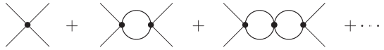
Figure 1: Two-body amplitude in the non-relativistic theory. The filled dots denote the full four-particle vertex that can be read off from the interaction Lagrangian. This vertex is a low-energy polynomial.

Next, let us consider the interactions in the two-particle sector. The full Lagrangian consists of an infinite tower of terms with zero, two,…derivatives in the interaction part

$${\cal L}={\cal L}_{\sf kin}+{\cal L}_{0}+{\cal L}_{2}+\cdots\,.$$ (4)

The lowest-order term is given by

$${\cal L}_{0}=C_{0}\phi^{\dagger}\phi^{\dagger}\phi\phi\,.$$ (5)

The coupling $C_{0}$ can be easily related to the two-body S-wave scattering lengths $a_{0}$ through the matching condition.

As usual, calculating the two-particle scattering amplitude for the process $p_{1}+p_{2}\to q_{1}+q_{2}$ with this Lagrangian amounts to summing up all bubble diagrams, see Fig. 1. In the S-wave amplitude, this gives:

$$T_{0}=(4C_{0})+(4C_{0})^{2}\frac{1}{2}\,I+(4C_{0})^{3}\frac{1}{4}\,I^{2}+\cdots=\frac{1}{(4C_{0})^{-1}-\frac{1}{2}\,I}\,.$$ (6)

Here, $I$ denotes a loop integral

$$I=\int\frac{d^{D}k}{(2\pi)^{D}i}\,\frac{1}{2w_{v}(k)(w_{v}(k)-vk-i\varepsilon)}\,\frac{1}{2w_{v}(P-k)(w_{v}(P-k)-v(P-k)-i\varepsilon)}\,,$$ (7)

and $P=p_{1}+p_{2}=q_{1}+q_{2}$ is the total CM momentum of a particle pair.

Before the evaluation of the above integral the following remarks are in order. First of all, the integrals are ultraviolet-divergent and should be regularized. We use dimensional regularization throughout this paper. This is however not sufficient for ensuring the preservation of counting rules in the loops. To this end, the so-called threshold expansion (see, e.g., Beneke:1997zp ) should be applied to the loops. One namely first uses the identity

$$\frac{1}{2w_{v}(k)(w_{v}(k)-vk-i\varepsilon)} = \frac{w_{v}(k)+vk}{2w_{v}(k)(m^{2}-k^{2}-i\varepsilon)}$$ (8)

$$= \frac{1}{m^{2}-k^{2}-i\varepsilon}-\frac{1}{2w_{v}(k)(w_{v}(k)+vk-i\varepsilon)}\,,$$

and a similar identity for the second propagator. Substituting these expression in Eq. (7), one gets four terms. Furthermore, the threshold expansion is applied in the vicinity of the particle poles, $vk=w_{v}(k)$ and $v(P-k)=w_{v}(P-k)$, respectively. Moreover, it is assumed that the “three-momenta” with respect to the quantization axis $v^{\mu}$, defined as $k_{\perp}^{\mu}=k^{\mu}-v^{\mu}vk$ and $(P-k)_{\perp}^{\mu}=(P-k)^{\mu}-v^{\mu}v(P-k)$ are small as compared to the particle mass $m$. This means that the second term in the above expression can be expanded as

$$-\frac{1}{2w_{v}(k)(w_{v}(k)+vk-i\varepsilon)} = -\frac{1}{4w_{v}^{2}(k)}-\frac{w_{v}(k)-vk}{8w_{v}^{3}(k)}+\cdots$$ (9)

$$= -\frac{1}{4m^{2}}+\frac{k_{\perp}^{2}}{4m^{4}}+\cdots-\frac{m-vk}{8m^{3}}+\cdots\,,$$

where the relation $w_{v}^{2}(k)=m^{2}-k_{\perp}^{2}$ has been used. A similar expansion can be written down for the second propagator. It is now immediately seen that only one term contributes to $I$ after the threshold expansion since, in the other terms, the integrand becomes a low-energy polynomial that leads to a vanishing integral in dimensional regularization. Hence, after performing the threshold expansion, we get:

$$I=I(s)=\int\frac{d^{D}k}{(2\pi)^{D}i}\,\frac{1}{(m^{2}-k^{2})(m^{2}-(P-k)^{2})}=\mbox{const}+\frac{\sigma}{16\pi^{2}}\,\ln\left(\frac{\sigma-1}{\sigma+1}\right)\,,$$ (10)

where

$$s=P^{2}\,,\quad\quad\sigma=\left(1-\frac{4m^{2}}{s+i\varepsilon}\right)^{1/2}\,.$$ (11)

The renormalization prescription is chosen so that $I(s)$ vanishes at the two-particle threshold $s=4m^{2}$.

The expression of the loop function, given in Eq. (10), is explicitly Lorentz-invariant (depends on the variable $s$ only). It also differs from the expression used in Refs. Colangelo:2006va ; Gasser:2011ju ; Bissegger:2008ff ; Bissegger:2007yq ; Gullstrom:2008sy . Namely, the imaginary parts of these two expressions coincide above elastic threshold that ensures two-body unitarity. Moreover, their difference is a low-energy polynomial with real coefficients and, hence, the choice of the loop function in a form given by Eq. (10) is as legitimate as the choice made earlier in Refs. Colangelo:2006va ; Gasser:2011ju ; Bissegger:2008ff ; Bissegger:2007yq ; Gullstrom:2008sy – these two correspond to a different renormalization prescription in the effective theory. Below, we shall stick to the definition given in Eq. (10). It has the advantage that the loop function is real and non-singular below threshold, whereas the original definition leads to a spurious singularity at $s=0$ and to an imaginary part below this value (we remind the reader that the point $s=0$ lays already outside the region of the applicability of the NREFT, so the question about the consistency of the approach does not arise here).

Note also that the original derivation given in the above papers was much shorter – there, one first integrated over the variable $k^{0}$ and then manipulated the integrand, depending on the three-momenta only. In case of arbitrary $v^{\mu}$, the dependence of the integrand on $k^{0}$ is more complicated. In principle, in the infinite volume, one could first perform a Lorentz boost that brings the vector $v^{\mu}$ to $v_{0}^{\mu}$ and then repeat the steps outlined in these papers. The result will of course be the same. We however stick to this derivation that can be applied in a finite volume without much ado.

In the following, it will be useful to rewrite the loop function as

$$I(s)=J(s)+\frac{i\sigma}{16\pi}\,.$$ (12)

Here, as mentioned before, the function $J(s)$ is a low-energy polynomial with real coefficients.

2.2 Terms with higher derivatives

The terms with higher derivatives, present in the Lagrangian, are of two types. The terms of the first type correspond to the effective-range expansion in a given partial wave (S-wave, in our case), and the terms of a second type describe higher partial waves.

Let us start with the former. The Lagrangian

$${\cal L}_{2}=C_{2}\biggl{\{}\bigl{(}(w_{\mu}\phi)^{\dagger}(w^{\mu}\phi)^{\dagger}\phi\phi-m^{2}\phi^{\dagger}\phi^{\dagger}\phi\phi\bigr{)}+\mbox{h.c.}\biggr{\}}$$ (13)

encodes the term related to the $S$-wave effective range $r_{0}$. Here,

$$w^{\mu}=v^{\mu}w_{v}+i\partial_{\perp}^{\mu}\,,\quad\quad\partial_{\perp}^{\mu}=\partial^{\mu}-v^{\mu}v\partial\,.$$ (14)

Furthermore, the tree amplitude in a theory consists of the contributions from ${\cal L}_{0}\,,\,{\cal L}_{2}\,,\ldots$, see Eqs. (4), (2.1) and (13):

$$T_{\sf tree}=T^{(0)}_{\sf tree}+T^{(2)}_{\sf tree}+\cdots\,.$$ (15)

As we already know, at lowest order,

$$T^{(0)}_{\sf tree}=4C_{0}\,.$$ (16)

Using now Eq. (13), it is straightforward to derive that, on mass shell,

$$T^{(2)}_{\sf tree}=4C_{2}\bigl{(}s-4m^{2}\bigr{)}\,,$$ (17)

where $s=(\tilde{p}_{1}+\tilde{p}_{2})^{2}=(\tilde{q}_{1}+\tilde{q}_{2})^{2}$, and $\tilde{p}_{i}^{\mu}=v^{\mu}w_{v}(p_{i})+p_{i\perp}^{\mu}$ (similarly for $\tilde{q}_{i}^{\mu}$ and any other vector). On the mass shell, where $w_{v}(p_{i})=vp_{i}$, $w_{v}(q_{i})=vq_{i}$ and, consequently, $\tilde{p}_{i}=p_{i}$, $\tilde{q}_{i}=q_{i}$, it also follows that $s=(p_{1}+p_{2})^{2}=(q_{1}+q_{2})^{2}$.

It is now crystal clear, how things proceed at higher orders. The tree-level amplitude in the S-wave represents a Taylor series in $s-4m^{2}$:

$$T^{\sf S-wave}_{\sf tree}=4C_{0}+4C_{2}(s-4m^{2})+4C_{4}(s-4m^{2})^{2}+\cdots\,,$$ (18)

All this is fine at tree level, on the mass shell. In the bubble sum, however, the intermediate particles are off the mass shell. Consider, for example the process $p_{1}+p_{2}\to k_{1}+k_{2}$, where $p_{i}^{2}=m^{2}$ and $k_{i}^{2}\neq m^{2}$. Then, $s_{p}=(\tilde{p}_{1}+\tilde{p}_{2})^{2}$ is not equal to $s_{k}=(\tilde{k}_{1}+\tilde{k}_{2})^{2}$, even if the relation $p_{1}+p_{2}=k_{1}+k_{2}$ always holds. Furthermore, the difference between $s_{p}$ and $s_{k}$ is proportional to $w_{v}(p_{1})+w_{v}(p_{2})-w_{v}(k_{1})-w_{v}(k_{2})$. Carrying out now the contour integration, one can straightforwardly ensure that such a term in the numerator cancels exactly with the denominator. One is left with a low-energy polynomial, and the integral over this polynomial vanishes in dimensional regularization. Therefore, replacing $s_{k}$ by $s_{p}=s$ everywhere in the numerator is justified. One may finally conclude that one could consistently pull out the numerator from the integral and evaluate it on shell. This results in the following S-wave amplitude:

$$T_{0}(s)=\frac{1}{(T^{\sf S-wave}_{\sf tree})^{-1}-\frac{1}{2}\,I(s)}.$$ (19)

Just above threshold, $s>4m^{2}$, one may rewrite this expression as

$$T_{0}(s)=\frac{16\pi\sqrt{s}}{16\pi\sqrt{s}((T^{\sf S-wave}_{\sf tree})^{-1}-\frac{1}{2}\,J(s))-ip(s)}\,,\quad\quad p(s)=\sqrt{\frac{s}{4}-m^{2}}\,.$$ (20)

Thus, just above threshold, the tree amplitude can be related to the S-wave scattering phase shift

$$16\pi\sqrt{s}((T^{\sf S-wave}_{\sf tree})^{-1}-\frac{1}{2}\,J(s))=p(s)\cot\delta_{0}(s)\,.$$ (21)

Expanding both sides in powers of $(s-4m^{2})$, one may carry out the matching of the constants $C_{0},C_{2},\ldots$ and the effective-range parameters in the S-wave $a_{0},r_{0},\ldots$. The lowest-order relation $C_{0}=-8\pi ma_{0}$ is the same as in Refs. Colangelo:2006va ; Gasser:2011ju – the modifications emerge, starting from the second order only.

Considering higher partial waves is a bit more subtle because the pertinent amplitudes depend on the directions of momenta as well. In the simple model considered, there is no P-wave. The lowest-order contribution of the D-wave is captured by the Lagrangian

$${\cal L}_{4} = {\cal L}_{4}^{\sf S}+{\cal L}_{4}^{\sf D}\,,$$

$${\cal L}_{4}^{\sf S} = 4C_{4}\biggl{(}\bigl{(}(w_{\mu}\phi)^{\dagger}(w^{\mu}\phi)^{\dagger}-m^{2}\phi^{\dagger}\phi^{\dagger}\bigr{)}\bigl{(}(w_{\nu}\phi)(w^{\nu}\phi)-m^{2}\phi\phi\bigr{)}\biggr{)}\,,$$

$${\cal L}_{4}^{\sf D} = \frac{5}{2}\,D_{4}\biggl{(}3(w_{\mu}\phi)^{\dagger}(w_{\nu}\phi)^{\dagger}(w^{\mu}\phi)(w^{\nu}\phi)-(w_{\mu}\phi)^{\dagger}(w^{\mu}\phi)^{\dagger}(w_{\nu}\phi)(w^{\nu}\phi)$$ (22)

$$- \frac{m^{2}}{2}\,\bigl{(}(w_{\mu}\phi)^{\dagger}(w^{\mu}\phi)^{\dagger}\phi\phi+\mbox{h.c.}\bigr{)}-m^{4}\phi^{\dagger}\phi^{\dagger}\phi\phi\biggr{)}\,.$$

The contribution from ${\cal L}_{4}^{\sf S}$ in the S-wave amplitude is already shown in Eq. (18). The contribution of the second term contributes to the on-shell tree amplitude in the D-wave:

$$T^{\sf D-wave}_{\sf tree} = \frac{5}{2}\,D_{4}\biggl{(}6\bigl{(}(\tilde{p}_{1}\tilde{q}_{1})(\tilde{p}_{2}\tilde{q}_{2})+(\tilde{p}_{1}\tilde{q}_{2})(\tilde{p}_{2}\tilde{q}_{1})\bigr{)}-4(\tilde{p}_{1}\tilde{p}_{2})(\tilde{q}_{1}\tilde{q}_{2})$$ (23)

$$- 2m^{2}\bigl{(}(\tilde{p}_{1}\tilde{p}_{2})+(\tilde{q}_{1}\tilde{q}_{2})\bigr{)}-4m^{4}\biggr{)}+\cdots$$

$$= 4D_{4}p^{4}(s)(2\cdot 2+1)P_{2}(\cos\theta)+\cdots\,,$$

where $P_{\ell}(\cos\theta)$ stand for the Legendre polynomials, and

$$\cos\theta=\frac{t-u}{s-4m^{2}}\,.$$ (24)

Here $s,t,u$ denote usual Mandelstam variables. Note that we have already used Lorentz invariance – the above expression does not depend on the vector $v^{\mu}$.

Next, let us consider summing up all bubble diagrams in the D-wave amplitude. The second iteration, for example, can be written as

second iteration $$= \int\frac{d^{D}k_{1}}{(2\pi)^{D}i}\,\frac{d^{D}k_{2}}{(2\pi)^{D}i}\,(2\pi)^{D}\delta^{D}(p_{1}+p_{2}-k_{1}-k_{2})$$ (25)

$$\times T^{\sf D-wave}_{\sf tree}(\tilde{p}_{1},\tilde{p}_{2};\tilde{k}_{1},\tilde{k}_{2})D(k_{1})D(k_{2})T^{\sf D-wave}_{\sf tree}(\tilde{k}_{1},\tilde{k}_{2};\tilde{q}_{1},\tilde{q}_{2})\,.$$

Here, $D(k)$ denotes the free propagator, see Eq. (2.1).

Furthermore, since $p_{i},q_{i}$ are on the mass shell, $\tilde{p}_{i}^{\mu}=p_{i}^{\mu}$ and $\tilde{q}_{i}^{\mu}=q_{i}^{\mu}$. On the contrary, $\tilde{k}_{i}^{\mu}=k_{i}^{\mu}+v^{\mu}(w_{v}(k_{i})-vk_{i})\neq k_{i}^{\mu}$. The additional term cancels with the denominator in $D(k_{i})$, leaving us, after performing the contour integral, with an integral over the low-energy polynomial that vanishes in the dimensional regularization. Hence, a replacement $\tilde{k}_{i}^{\mu}\to k_{i}^{\mu}$ in the numerator is justified. Next, using Eq. (8), we may rewrite the above equation as:

second iteration $$= \int\frac{d^{D}k_{1}}{(2\pi)^{D}i}\,\frac{d^{D}k_{2}}{(2\pi)^{D}i}\,(2\pi)^{D}\delta^{D}(p_{1}+p_{2}-k_{1}-k_{2})$$ (26)

$$\times \frac{T^{\sf D-wave}_{\sf tree}(p_{1},p_{2};k_{1},k_{2})T^{\sf D-wave}_{\sf tree}(k_{1},k_{2};q_{1},q_{2})}{(m^{2}-k_{1}^{2}-i\varepsilon)(m^{2}-k_{2}^{2}-i\varepsilon)}\,.$$

It is seen that this integral is written down in a completely Lorentz-invariant form. In order to evaluate it, we perform the boost to the center-of-mass frame of two particles. In this system, the angular integral can be readily done, yielding the Legendre polynomial. Pulling again the numerator out from the integral, we finally get:

$$\mbox{second iteration}=(4D_{4}p^{4}(s))^{2}\frac{1}{2}\,I(s)(2\cdot 2+1)P_{2}(\cos\theta)\,.$$ (27)

Now, it is easy to write down the result for the D-wave amplitude, summing up the bubbles at all orders:

$$T_{2}(s)=\frac{p^{4}(s)}{(4D_{4})^{-1}-\frac{1}{2}\,p^{4}(s)I(s)}\,.$$ (28)

Furthermore, it is already clear that, if higher-order terms are taken into account, the D-wave amplitude takes the form

$$T_{2}(s)=\frac{p^{4}(s)}{(T^{\sf D-wave}_{\sf tree})^{-1}-\frac{1}{2}\,p^{4}(s)I(s)}\,,\quad\quad T^{\sf D-wave}_{\sf tree}=4D_{4}+4D_{6}(s-4m^{2})+\cdots\,.$$ (29)

The matching condition in the D-wave is given by:

$$16\pi\sqrt{s}\bigl{(}(T^{\sf D-wave}_{\sf tree})^{-1}-\frac{1}{2}\,p^{4}(s)J(s)\bigr{)}=p^{5}(s)\cot\delta_{2}(s)\,.$$ (30)

We are now in a position to write down the expression of the complete amplitude:

$$T(s,t)=\sum_{\ell}(2\ell+1)P_{\ell}(\cos\theta)T_{\ell}(s)\,,\quad\quad T_{\ell}(s)=\frac{p^{2\ell}(s)}{(T^{\ell}_{\sf tree})^{-1}-\frac{1}{2}\,p^{2\ell}(s)I(s)}\,,$$ (31)

where $T^{\ell}_{\sf tree}$ represents a low-energy polynomial in the variable $(s-4m^{2})$. The matching condition

$$16\pi\sqrt{s}\bigl{(}(T^{\ell}_{\sf tree})^{-1}-\frac{1}{2}\,p^{2\ell}(s)J(s)\bigr{)}=p^{2\ell+1}(s)\cot\delta_{\ell}(s)$$ (32)

allows one to perform the matching of the couplings in the low-energy effective Lagrangian to the parameters of the effective-range expansion in all partial waves.

In conclusion, we would like to note that, albeit we have started with an explicitly non-covariant Lagrangian, the physical amplitudes are relativistic invariant, i.e., do not depend on the vector $v^{\mu}$. This statement is by no means trivial. The relativistic invariance could be achieved, because a) the interaction Lagrangian of four pions has a particularly simple form – it is a bunch of local vertices, and b) the threshold expansion has been applied in the calculation of Feynman integrals. In the three-particle sector, neither of these conditions hold. The result depends on $v^{\mu}$ and the relativistic invariance is achieved, when $v^{\mu}$ is fixed in terms of the external momenta. Below, in Sect. 3, we shall consider this issue in detail.

2.3 Introducing dimers

As in Refs. Hammer:2017uqm ; Hammer:2017kms , we shall introduce dimer fields in the Lagrangian in order to trade four-particle interactions in favor of particle-dimer vertices. This will lead to a significant simplification in the description of the three-particle systems, since the bookkeeping of different diagrams is made much easier in the particle-dimer picture. Note also that, according to our philosophy, introducing a dimer does not necessarily mean that a physical dimer (two-particle bound state) should exist, albeit this may still be the case. Thus, the particle-dimer formalism is not an approximation – rather, it is a different choice of variables in the path integral, equivalent to the original formulation. Note also that, instead of a single dimer field, we in fact have to introduce an infinite bunch of dimer fields with different spin, corresponding to different angular momenta $\ell$ in the two-particle system.

Let us again start with the S-wave, and consider the Lagrangian

$${\cal L}_{\sf S} = \phi^{\dagger}2w_{v}(i(v\partial)-w_{v})\phi+\sigma T^{\dagger}T$$ (33)

$$+ \biggl{(}\frac{1}{2}\,T^{\dagger}\bigl{(}f_{0}\phi\phi+f_{2}\bigl{(}(w_{\mu}\phi)(w^{\mu}\phi)-m^{2}\phi\phi\bigr{)}+\cdots\bigr{)}+\mbox{h.c.}\biggr{)}+\cdots\,.$$

Here, $T$ denotes a (scalar) dimer field which does not possess a kinetic term, and $\sigma=\pm 1$, depending on the sign of the coupling $C_{0}$. It is easily seen that, integrating out the dimer field in the path integral, we arrive at the four-particle local coupling one has started with. It is then a simple algebraic exercise to express the new couplings $f_{0},f_{2},\ldots$ through the $C_{0},C_{2},\ldots$ and $\sigma$.

The inclusion of the dimers with higher spins proceeds similarly – one has to merely reformulate the construction of Ref. Hammer:2017kms in the present relativistic setting. To this end, we introduce the tensor dimer fields $T_{\mu_{1},\cdots,\mu_{\ell}}$, corresponding to the angular momentum $\ell$. These fields are symmetric under the permutation of each pair of indices, traceless in each pair of indices and obey the constraints:

$$v^{\mu_{i}}T_{\mu_{1},\cdots,\mu_{\ell}}=0\,,\quad\quad i=1,\cdots,\ell\,.$$ (34)

These constraints leave the correct number of independent degrees of freedom, equal to $2\ell+1$.. The Lagrangian in the two-particle sector can be written as:

$${\cal L}=\phi^{\dagger}2w_{v}(i(v\partial)-w_{v})\phi+\sum_{\ell=0}^{\infty}\sigma_{\ell}T^{\dagger}_{\mu_{1},\cdots,\mu_{\ell}}T^{\mu_{1},\cdots,\mu_{\ell}}+\frac{1}{2}\,\sum_{\ell=0}^{\infty}\bigl{(}T^{\dagger}_{\mu_{1},\cdots,\mu_{\ell}}O^{\mu_{1},\cdots,\mu_{\ell}}+\mbox{h.c.}\bigr{)}\,,\quad\quad$$ (35)

where $\sigma_{\ell}=\pm 1$ and $O^{\mu_{1},\cdots,\mu_{\ell}}$ are the relativistic two-particle operators, corresponding to the orbital momentum $\ell$. These operators can be easily constructed, based on the explicit expression of the spherical functions. For example, the lowest-order operator in the D-wave is given by:

$$O^{\mu\nu} = g_{0}\biggl{(}\frac{3}{2}\,(\phi({\bar{w}}_{\perp}^{\mu}{\bar{w}}_{\perp}^{\nu}\phi)-({\bar{w}}_{\perp}^{\mu}\phi)({\bar{w}}_{\perp}^{\nu}\phi))$$ (36)

$$- \frac{1}{2}\,(g^{\mu\nu}-v^{\mu}v^{\nu})(\phi({\bar{w}}_{\perp}^{\lambda}\bar{w}_{\perp\lambda}\phi)-({\bar{w}}_{\perp}^{\lambda}\phi)(\bar{w}_{\perp\lambda}\phi))\biggr{)}\,,$$

where ${\bar{w}}_{\perp}^{\mu}=\bar{w}^{\mu}-v^{\mu}(v\bar{w})$ and $\bar{w}^{\mu}$ denotes the operator $w^{\mu}$ which is boosted in the CM system of two particles with respect to the vector $v^{\mu}$. Under this, we mean that the boosted total momentum of two particles on mass shell is parallel to the vector $v^{\mu}$. Needless to say that, in a particular case $v^{\mu}=v_{0}^{\mu}$, we get the usual definition of the two-particle CM frame.

The transformation of $w^{\mu}$ to $\bar{w}^{\mu}$ is given through the matrix

$$\bar{w}^{\mu}=\Lambda^{\mu}_{\nu}w^{\nu}\,.$$ (37)

It is easier to work in the momentum space. Let $\tilde{p}_{1,2}$ be the on-mass shell momenta of individual particles. Then, $P=\tilde{p}_{1}+\tilde{p}_{2}$ is the total on-mass shell momentum of the pair. The boost makes the vector $P^{\mu}$ parallel to $v^{\mu}$, that is

$$\bar{P}^{\mu}=\Lambda^{\mu}_{\nu}P^{\nu}=\sqrt{P^{2}}v^{\mu}\,,\quad\quad{\Lambda^{-1}}^{\mu}_{\nu}v^{\nu}=\frac{1}{\sqrt{P^{2}}}\,P^{\mu}\,.$$ (38)

This leads to

$${\bf v}^{2}{\bf\bar{P}}={\bf v}({\bf v}{\bf\bar{P}})\,,\quad\quad|{\bf v}|\bar{P}^{0}=v^{0}|{\bf\bar{P}}|\,.$$ (39)

The above identities suffice to express the matrix elements of $\Lambda^{\mu}_{\nu}$ in terms of the vectors $v^{\mu},P^{\mu}$. Substituting back into the Lagrangian, one should replace the components of $P^{\mu}$ by the operators $w^{\mu}$, acting on the $\phi$ fields. The resulting explicit expression is rather voluminous and non-local. It is always implicitly assumed that, in actual calculations, the pertinent expressions are expanded in the inverse powers of the mass $m$, the result is integrated in dimensional regularization and summed up back to all orders. Also, we do not display here the explicit expression of the matrix $\Lambda^{\mu}_{\nu}$, because it will never be needed.

In the momentum space, the lowest-order D-wave two-particle-dimer vertex is given by

$$\Gamma^{\mu\nu}(p)=-4g_{0}\biggl{(}\frac{3}{2}\,\bar{p}_{\perp}^{\mu}\bar{p}_{\perp}^{\nu}-\frac{1}{2}\,(g^{\mu\nu}-v^{\mu}v^{\nu})(\bar{p}_{\perp})^{2}\biggr{)}\,,$$ (40)

where $\bar{p}^{\mu}=\frac{1}{2}\,(\bar{p}_{1}^{\mu}-\bar{p}_{2}^{\mu})$. Now, integrating out the dimer field $T^{\mu\nu}$, we arrive at

$$\Gamma^{\mu\nu}(p)\Gamma_{\mu\nu}(q)=16g_{0}^{2}\biggl{(}\frac{9}{4}\,(\bar{p}_{\perp}\bar{q}_{\perp})^{2}-\frac{3}{4}\,(\bar{p}_{\perp})^{2}(\bar{q}_{\perp})^{2}\biggr{)}\,.$$ (41)

Furthermore,

$$\bar{p}_{\perp}^{\mu}=\bar{p}^{\mu}-v^{\mu}(v\bar{p})=\bar{p}^{\mu}-v^{\mu}(\Lambda^{-1}v)_{\nu}p^{\nu}=\bar{p}^{\mu}-\frac{1}{2\sqrt{P^{2}}}\,v^{\mu}((\tilde{p}_{1}+\tilde{p}_{2})(\tilde{p}_{1}-\tilde{p}_{2}))=\bar{p}^{\mu}\,.\quad\quad$$ (42)

Using Lorentz invariance, one can transform back to the laboratory frame:

$$\Gamma^{\mu\nu}(p)\Gamma_{\mu\nu}(q) = 24g_{0}^{2}\biggl{(}\frac{3}{2}\,(pq)^{2}-\frac{1}{2}\,p^{2}q^{2}\biggr{)}=\frac{3}{2}\,g_{0}^{2}\biggl{(}\frac{3}{2}\,(t-u)^{2}-\frac{1}{2}\,(s-4m^{2})^{2}\biggr{)}$$ (43)

$$= 24g_{0}^{2}p^{4}(s)P_{2}(\cos\theta)\,.$$

This result is similar to Eq. (23) and gives a matching condition for the variable $g_{0}$. Inclusions of higher orders in the effective-range expansion, as well as higher partial waves is now straightforward and will not be written down in detail. The only difference to the “conventional” case with $v^{\mu}=v_{0}^{\mu}$ is that all momenta are boosted to the CM frame with respect to $v^{\mu}$, i.e., the total momentum is parallel to $v^{\mu}$ after the boost. Further, instead of three-momenta in the boosted frame, the transverse components $p_{\perp}$ are considered, and the covariant expression $v^{\mu}v^{\nu}-g^{\mu\nu}$ replaces the three-dimensional Kronecker delta in the boosted frame. Last but not least, we wish to reiterate that, unlike the original formulation of the RFT formalism, the boost is always well defined in the NREFT framework. This happens because we work with the on-shell particles.

Finally note that the two-body on-shell amplitude, given in Eq. (31) can be rewritten in the following form

$$T(s,t)=4\pi\sum_{\ell m}\mathscr{Y}_{\ell m}({\bf\tilde{p}})\frac{1}{(T^{\ell}_{\sf tree}(s))^{-1}-\frac{1}{2}\,p^{2\ell}(s)I(s)}\,\mathscr{Y}^{*}_{\ell m}({\bf\tilde{q}})\,,$$ (44)

where

$${\bf\tilde{p}}={\bf\bar{p}}-{\bf v}\frac{{\bf\bar{p}}{\bf v}}{{\bf v}^{2}}+{\bf v}\frac{\bar{p}^{0}}{{\bf v}^{2}}\,,\quad\quad{\bf\tilde{q}}={\bf\bar{q}}-{\bf v}\frac{{\bf\bar{q}}{\bf v}}{{\bf v}^{2}}+{\bf v}\frac{\bar{q}^{0}}{{\bf v}^{2}}\,,\quad\quad{\bf\tilde{p}}{\bf\tilde{q}}=-\bar{p}_{\mu}\bar{q}^{\mu}\,,$$ (45)

and

$$\mathscr{Y}_{\ell m}({\bf k})=|{\bf k}|^{\ell}Y_{\ell m}(\hat{k})\,,\quad\quad\hat{k}=\frac{\bf k}{|{\bf k}|}\,.$$ (46)

Note that, in case of $v^{\mu}=v_{0}^{\mu}$, the above definition of the boosted amplitude coincides with the boost introduced in Wu:2015evh ; Li:2021mob ; Wu . Within this prescription the boosted three-momenta are always well-defined, even for $s<0$.

3 Three-body sector

3.1 Particle-dimer Lagrangian

The construction of the particle-dimer Lagrangian that describes short-range three-particle interactions, proceeds analogously to the case of the two-particle Lagrangian, except three differences. First, a dimer and $\phi$ are not identical particles and hence all (not only even) partial waves are allowed. Second, in difference with $\phi$, dimers have spin. And third, in the particle-dimer system one cannot use equations of motion in order to reduce the number of the independent terms in the Lagrangian. The dimers, in general, are unphysical “particles” and do not have a fixed mass.

Let us again start with a scalar dimer. The tree-level particle-dimer scattering amplitude depends on the following kinematic variables:

$$s=(p+P)^{2}=(q+Q)^{2}\,,\quad t=(p-q)^{2}=(P-Q)^{2}\,,\quad\sigma_{p}^{2}=P^{2}\,,\quad\sigma_{q}^{2}=Q^{2}\,,$$ (47)

where $p,q$ and $P,Q$ are the momenta of incoming/outgoing particles and incoming/outgoing dimers, respectively. Consistent counting rules can be imposed, for example, assuming:

$$\Delta = s-9m^{2}=O(\epsilon^{2})\,,\quad\quad t=O(\epsilon^{2})\,,$$

$$\Delta_{p} = \sigma_{p}^{2}-4m^{2}=O(\epsilon^{2})\,,\quad\quad\Delta_{q}=\sigma_{q}^{2}-4m^{2}=O(\epsilon^{2})\,,$$ (48)

where $\epsilon$ is a generic small parameter, and all transverse momenta count as $p_{\perp}=O(\epsilon)$.

Expanding the tree amplitude in Taylor series, we get:

$$T_{d}^{\sf tree}(s,t,\sigma_{p}^{2},\sigma_{q}^{2})=x_{0}+x_{1}(s-9m^{2})+x_{2}t+x_{3}(\sigma_{p}^{2}+\sigma_{q}^{2}-8m^{2})+O(\epsilon^{4})\,.$$ (49)

Here, we have additionally used the invariance under time reversal that implies the interchange of the initial and final momenta. In the tree-level amplitude all coefficients $x_{0},x_{1},\ldots$ are real due to unitarity.

Furthermore, the couplings $x_{0},x_{1},\ldots,$ determined from the tree-level matching, are not all independent. Indeed, the particle-dimer Lagrangian is used to calculate the three-particle amplitude, and the matching is performed for the latter. The couplings (or the linear combinations thereof), which do not contribute to the on-shell three-particle amplitude, are redundant and can be dropped. In order to obtain the three-particle scattering amplitude from the particle-dimer scattering amplitude, one has to equip the external dimer legs with two-particle-dimer vertices and sum up over all permutations in the initial as well as final state. At order $\epsilon^{2}$, it suffices to consider the vertex $f=f_{0}+\frac{1}{2}\,f_{2}(\sigma^{2}-4m^{2})$, see Eq. (33). Here, $\sigma^{2}$ stands for the four-momentum square of a dimer. Since any of the initial or final particles can be a spectator, one has to equip the quantities $\Delta_{p,q}$ and $t$ by indices $i,j=1,2,3$ that label spectator particles, and sum over these indices. Thus, one has to define:

$$\Delta_{p}^{i}=P_{i}^{2}-4m^{2}\,,\quad\quad\Delta_{q}^{i}=Q_{i}^{2}-4m^{2}\,,\quad\quad t^{ij}=(p_{i}-q_{j})^{2}\,.$$ (50)

These obey the following kinematic identities on mass shell, see also Ref. Blanton:2019igq :

$$\sum_{i=1}^{3}\Delta_{p}^{i}=\sum_{i=1}^{3}\Delta_{q}^{i}=\Delta\,,\quad\quad\sum_{j=1}^{3}t^{ij}=\Delta_{p}^{i}-\Delta\,,\quad\quad\sum_{i=1}^{3}t^{ij}=\Delta_{q}^{j}-\Delta\,.$$ (51)

The three-particle amplitude is given by

$$T_{3}^{\sf tree}=\sum_{i,j=1}^{3}f({\sigma_{p}^{i}}^{2})T_{d}^{\sf tree}(s,t^{ij},{\sigma_{p}^{i}}^{2},{\sigma_{q}^{j}}^{2})f({\sigma_{q}^{j}}^{2})+O(\epsilon^{4})\,.$$ (52)

Taking into account the above identities, it is straightforward to ensure that only two independent terms survive in the tree-level three-particle amplitude at this order:

$$T_{3}^{\sf tree}=z_{0}+z_{1}\Delta+O(\epsilon^{2})\,.$$ (53)

This agrees with the result of Ref. Blanton:2019igq . Moreover, as shown in Bedaque:2002yg , in the particle-dimer formalism it is possible to trade the terms of the type $\Delta_{p}+\Delta_{q}$ and $\Delta$ for each other. Thus our result confirms the findings of Ref. Bedaque:2002yg as well. To summarize, only one coupling out of $x_{1},x_{2},x_{3}$ is independent and, without the loss of generality, one may assume, say, $x_{2}=x_{3}=0$ (Note also that in Refs. Hammer:2017uqm ; Hammer:2017kms we have written down an energy-independent next-to-leading order driving term containing ${\bf p}^{2}+{\bf q}^{2}$. In the present context, it corresponds to the choice $x_{1}=x_{2}=0$ and $x_{3}\neq 0$.). Finally, note that a similar analysis can be carried out at higher orders. We do not consider here this rather straightforward exercise which, at order $\epsilon^{4}$, again reproduces the result of Ref. Blanton:2019igq .

Here one should however note that all the above analysis was limited to the case when a physical dimer does not exist. In case this is not true, the following line of reasoning can be applied. Let us go back to Eq. (49). In this case, $\sigma_{p}^{2}$ and $\sigma_{q}^{2}$ are not independent kinematic variables anymore, being fixed to the dimer mass squared. On the contrary, the derivative couplings $x_{1},x_{2}$ can be independently matched to the S-wave effective range and the P-wave scattering length of the particle-dimer scattering.

Furthermore, note that all discussions up to now were restricted to the tree level. Owing to the fact that the use of the cutoff regularization in the Faddeev equation leads to the breakdown of naive counting rules that can be rectified only by adjusting the renormalization prescription, studying the independence of $x_{1},x_{2},x_{3}$ in general is a more subtle issue. In this case, we find it safe to include all couplings – after all, using (possibly) an overcomplete set of operators in the Lagrangian is certainly not a mistake.

A final remark here concerns the situation, where the low-lying three-particle resonances exist. In this case, the assumption that the short-range part of the particle-dimer interaction is a low-energy polynomial in $s-9m^{2}$ might prove to be too restrictive, since the pertinent expansion has a very small radius of convergence, caused by a nearby resonance. A Laurent expansion of the short-range interaction, featuring a simple pole $\sim(s-s_{0})^{-1}$ with an unknown parameter $s_{0}$, describes the system in a more adequate fashion in this case.

Next, let us briefly dwell on the partial-wave expansion of the particle-dimer short-range tree amplitude. As seen, the $O(\epsilon^{2})$ amplitude contains only an S-wave contribution. At higher orders, one can define the scattering angle $\theta$, according to

$$t-2m^{2}=\frac{(s+m^{2}-\sigma_{p}^{2})(s+m^{2}-\sigma_{q}^{2})}{4s}-\frac{\lambda^{1/2}(s,m^{2},\sigma_{p}^{2})\lambda^{1/2}(s,m^{2},\sigma_{q}^{2})}{4s}\,\cos\theta\,.$$ (54)

Then, the expansion of the tree particle-dimer amplitude in the series of Legendre polynomials can be written down straightforwardly. Note that, at a given order in $\epsilon$, this expansion always contains a finite number of Legendre polynomials.

Having considered the scattering of a particle and a scalar dimer in a great detail, we now sketch the construction in case of a dimer with arbitrary integer spin. To this end, it is convenient to use a different basis for the dimer fields $T_{\mu_{1},\cdots,\mu_{\ell}}$, removing the redundant components. In order to achieve this, consider first the Lorentz transformation

$$\underline{\Lambda}^{\mu}_{\nu}v^{\nu}=v_{0}^{\mu}\,,\quad\quad\underline{T}_{\mu_{1},\cdots,\mu_{\ell}}=\underline{\Lambda}_{\mu_{1}}^{\nu_{1}}\cdots\underline{\Lambda}_{\mu_{\ell}}^{\nu_{\ell}}T_{\nu_{1},\cdots,\nu_{\ell}}\,.$$ (55)

The transformed field $\underline{T}$ is zero, if one of the indices $\mu_{1},\ldots,\mu_{\ell}$ is equal to zero, see Eq. (34). The space components can be directly related to the dimer field components $T_{\ell m}$ with $m=-\ell,\ldots,\ell$:

$$\underline{T}_{\mu_{1},\cdots,\mu_{\ell}}=\sum_{m=-\ell}^{\ell}c_{\mu_{1},\cdots,\mu_{\ell}}^{\ell m}T_{\ell m}\,.$$ (56)

The coefficients $c_{\mu_{1},\cdots,\mu_{\ell}}^{\ell m}$ are pure numbers and can be read off from the explicit expressions of the spherical functions. They are zero, if one of the $\mu_{i}$ is equal to zero.

A generic matrix element can be also boosted to the rest frame:

$$\langle p,(P,\mu_{1}^{\prime},\cdots,\mu_{\ell^{\prime}}^{\prime})|T_{d}^{\sf tree}|q,(Q,\mu_{1},\cdots,\mu_{\ell})\rangle=(\underline{\Lambda}^{-1})_{\mu_{1}^{\prime}}^{\nu_{1}^{\prime}}\cdots(\underline{\Lambda}^{-1})_{\mu_{\ell^{\prime}}^{\prime}}^{\nu_{\ell^{\prime}}^{\prime}}(\underline{\Lambda}^{-1})_{\mu_{1}}^{\nu_{1}}\cdots(\underline{\Lambda}^{-1})_{\mu_{\ell}}^{\nu_{\ell}}$$

$$\quad\quad\times\,\sum_{m^{\prime}=-\ell^{\prime}}^{\ell^{\prime}}\sum_{m=-\ell}^{\ell}c_{\nu_{1}^{\prime},\cdots,\nu_{\ell^{\prime}}^{\prime}}^{\ell^{\prime}m^{\prime}}c_{\nu_{1},\cdots,\nu_{\ell}}^{\ell m}\langle\underline{p},(\ell^{\prime}m^{\prime})|T_{d}^{\sf tree}|\underline{q},(\ell m)\rangle\,,$$ (57)

where $\underline{p}^{\mu},\underline{q}^{\mu}$ are the Lorentz-transformed momenta:

$$\underline{p}^{\mu}=\underline{\Lambda}^{\mu}_{\nu}p^{\nu}\,,\quad\quad\underline{q}^{\mu}=\underline{\Lambda}^{\mu}_{\nu}q^{\nu}\,,$$ (58)

and we anticipated that the total momentum of the system $K^{\mu}$ is proportional to $v^{\mu}$, so that the same Lorentz boost brings the considered matrix element to the CM frame.

The matrix element in the right-hand side can be expanded in partial waves:

$$\langle\underline{p},(\ell^{\prime}m^{\prime})|T_{d}^{\sf tree}|\underline{q},(\ell m)\rangle=4\pi\sum_{JM}\sum_{L^{\prime}L}\mathscr{Y}^{L^{\prime}\ell^{\prime}}_{JM}({\bf\underline{p}},m^{\prime})T_{JL^{\prime}L}(\Delta,\Delta_{p},\Delta_{q})\bigl{[}\mathscr{Y}^{L\ell}_{JM}({\bf\underline{q}},m)\bigr{]}^{*}\,.$$ (59)

Here,

$$\mathscr{Y}^{L\ell}_{JM}({\bf\underline{k}},m)=\langle L(M-m),\ell m|JM\rangle\mathscr{Y}_{L(M-m)}({\bf\underline{k}})$$ (60)

is the spherical function with spin $\ell$, which is given by an ordinary spherical function multiplied with the pertinent Clebsch-Gordan coefficient. Note that, for a generic $v^{\mu}$, the above expansion has a more complicated form, since an additional boost is needed to bring the matrix element to the CM frame first. Also, the above expressions show that in the partial-wave expansion of the three-particle amplitude one encounters two orbital momenta: 1) the orbital momentum of pairs which in the particle-dimer approach are represented by the dimer spin $\ell$, and 2) the orbital momentum between a pair and a spectator, which corresponds to the quantum number $L$. The introduction of dimers allows one to neatly separate the partial-wave expansion in these two orbital momenta. The quantity $J$ corresponds to a sum of these orbital momenta and is conserved.

Furthermore, the quantities $T_{JL^{\prime}L}(\Delta,\Delta_{p},\Delta_{q})$ are the low-energy polynomials, expanded up to a given order in $\epsilon$. Like in the case of a scalar dimer, some on-shell constraints will emerge between various low-energy couplings at a given order in $\epsilon$. We shall make no attempt here to write down these constraints in a general form. When needed, this can be most easily done on the case-by-case basis.

A further remark is due at this place, concerning the expression of the most general Lorentz-invariant short-range amplitude. Namely, in the construction of the invariant kinematic structures we have never used the vector $v^{\mu}$ which should be also included on general grounds. The excuse is provided by the fact that, at the end, we shall relate $v^{\mu}$ to the external momenta (in particular, we shall take it parallel to the total momentum of the three-particle system). In this case, all invariants that can be constructed with the use of $v^{\mu}$ can be expressed in terms of the already considered ones. Anticipating this fact, we did not write down such invariants at all.

This concludes the construction of a short-range tree-level particle-dimer scattering amplitude with initial and final dimers having any spins $\ell,\ell^{\prime}$. Construction of such an amplitude is equivalent to the construction of the particle-dimer Lagrangian. We do not make an attempt to display such a Lagrangian explicitly, because it is far more convenient to work directly with the momentum space amplitudes.

3.2 Faddeev equation for the particle-dimer amplitude

Now, we are ready to write down the Faddeev equation, describing the particle-dimer scattering, in an explicitly Lorentz-invariant form. In order to avoid cumbersome expressions that will only render the basic idea obscure, we shall first restrict ourselves to the S-wave interactions in both orbital momenta. As follows from the discussion above, including higher partial waves merely amounts to adding indices to some of the quantities in the expressions. This procedure can be readily carried out.

Let us start from the scalar dimer propagator:

$$i\langle 0|T[T(x)T^{\dagger}(y)]|0\rangle=\int\frac{d^{4}P}{(2\pi)^{4}}\,e^{-iP(x-y)}S(P^{2})\,,$$ (61)

where

$$S(P^{2})=\biggl{(}-\frac{1}{\sigma}\biggr{)}+\biggl{(}-\frac{1}{\sigma}\biggr{)}^{2}\Sigma(P^{2})+\cdots=-\frac{1}{\sigma+\Sigma(P^{2})}\,,$$ (62)

and

$$\Sigma(P^{2})=\int\frac{d^{D}k}{(2\pi)^{D}i}\,\frac{\frac{1}{2}\,f^{2}(\bar{P}^{2})}{2w_{v}(k)(w_{v}(k)-vk-i\varepsilon)\,2w_{v}(P-k)(w_{v}(P-k)-v(P-k)+i\varepsilon)}\,,$$

with

$$\bar{P}^{2}=(w_{v}(k)+w_{v}(P-k))^{2}+P_{\perp}^{2}\,,\quad\quad f(u)=f_{0}+\frac{1}{2}\,f_{2}(u-4m^{2})+\cdots\,.$$ (64)

Performing the threshold expansion and evaluating the expression in dimensional regularization, one gets:

$$\Sigma=\frac{1}{2}\,f^{2}(P^{2})I(P^{2})\,,$$ (65)

where $I(P^{2})$ is given in Eq. (10).

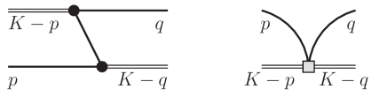
Figure 2: The kernel of the Faddeev equation. Double and single lines denote the dimers and particles, respectively. The dark blob describes a dimer-two-particle vertex, and a shaded box corresponds to the short-range part of the particle-dimer scattering.

Next, let us consider the tree-level particle-dimer scattering amplitude, which consists of two diagrams shown in Fig. 2. These are diagrams describing one-particle exchange and the local particle-dimer interaction. Furthermore, vertices in each diagram consist of an infinite number of terms, corresponding to the derivative operators in the Lagrangian. Thus, the tree-level amplitude is given by

$$T^{\sf tree}=\frac{f(s_{p})f(s_{q})}{2w_{v}(K-p-q)(w_{v}(p)+w_{v}(q)+w_{v}(K-p-q)-vK-i\varepsilon)}+T_{d}^{\sf tree}\,.$$ (66)

Here, $p,q$ are the four-momenta of the external particles, and $K$ is a total momentum of a particle-dimer pair. Hence, the four momenta of dimers are $P=K-p$ and $Q=K-q$. The short-range particle-dimer amplitude is given by Eq. (49). Furthermore, the kinematic variables $s_{p},s_{q}$ are given by

$$s_{p} = (w_{v}(p)+w_{v}(K-p-q))^{2}+(K-q)_{\perp}^{2}\,,$$

$$s_{q} = (w_{v}(q)+w_{v}(K-p-q))^{2}+(K-p)_{\perp}^{2}\,,$$ (67)

and, for any vector $a^{\mu}$, we have $a^{\mu}_{\perp}=a^{\mu}-v^{\mu}(va)$.

Furthermore, let us consider the difference:

$$s_{p}-\sigma_{q}^{2}=s_{p}-(K-q)^{2}=(w_{v}(p)+w_{v}(K-p-q))^{2}-(w_{v}(p)-v(K-p-q))^{2}$$ (68)

$$= (w_{v}(p)+w_{v}(K-p-q)+w_{v}(q)-vK)(w_{v}(p)+w_{v}(K-p-q)-w_{v}(q)+vK)\,.\quad\quad$$

A similar relation holds for the $s_{q}-\sigma_{p}^{2}=s_{q}-(K-p)^{2}$. Taking into account the fact that the function $f(u)$ is a low-energy polynomial in the variable $u-4m^{2}$, it is seen that the arguments $s_{p},s_{q}$ in these functions can be replaced by $\sigma_{q}^{2},\sigma_{p}^{2}$. In the difference, the denominator cancels and hence, it only modifies the regular part $T_{d}^{\sf tree}$. The fact that the modified short-range part now depends on the vector $v^{\mu}$, does not lead to any problem. One could merely ignore such $v$-dependent terms since, at the end, $v^{\mu}$ will be chosen proportional to $K^{\mu}$. Thus, one could write

$$\tilde{T}^{\sf tree}=\frac{f(\sigma_{p}^{2})f(\sigma_{q}^{2})}{2w_{v}(K-p-q)(w_{v}(p)+w_{v}(q)+w_{v}(K-p-q)-vK-i\varepsilon)}+\tilde{T}_{d}^{\sf tree}\,.$$ (69)

Note that the separate terms in Eqs. (66) and (69) are manifestly invariant, if the vector $v^{\mu}$ is also boosted along with all other vectors. This is different from the standard formulation, where $v^{\mu}$ is chosen along $v_{0}^{\mu}$ and does not transform under Lorentz transformations.

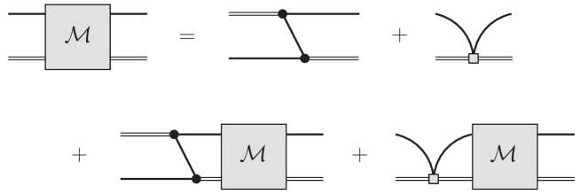
Figure 3: Faddeev equation for the particle-dimer scattering amplitude.

Graphically, the Faddeev equation for the particle-dimer scattering amplitude is depicted in Fig. 3. Denoting this amplitude by $\tilde{T}$, we have:

$$\tilde{T}(p,q)=\tilde{T}^{\sf tree}(p,q)+\int^{\Lambda_{v}}\frac{d^{3}k_{\perp}}{(2\pi)^{3}2w_{v}(k)}\,\tilde{T}^{\sf tree}(p,k)S((K-k)^{2})\tilde{T}(k,q)\,,$$ (70)

where

$$\int^{\Lambda_{v}}\frac{d^{3}k_{\perp}}{(2\pi)^{3}2w_{v}(k)}\,F(k)=\int\frac{d^{4}k}{(2\pi)^{3}}\,\delta(k^{2}-m^{2})\theta(\Lambda^{2}+k^{2}-(vk)^{2})F(k)\,.$$ (71)

Defining now

$$\tilde{T}(p,q) = f(\sigma_{p}^{2}){\cal M}(p,q)f(\sigma_{q}^{2})\,,$$

$$\tilde{T}^{\sf tree}(p,q) = f(\sigma_{p}^{2}){\cal Z}(p,q)f(\sigma_{q}^{2})\,,$$ (72)

we may finally rewrite the Faddeev equation as

$${\cal M}(p,q)={\cal Z}(p,q)+\int^{\Lambda_{v}}\frac{d^{3}k_{\perp}}{(2\pi)^{3}2w_{v}(k)}\,{\cal Z}(p,k)\tau((K-k)^{2}){\cal M}(k,q)\,.$$ (73)

Here, $\tau(z)$ is the physical two-body scattering matrix

$$\tau(z)=f^{2}(z)S(z)=\frac{1}{-\sigma f^{-2}(z)-\frac{1}{2}\,I(z)}=T_{0}(z)\,,$$ (74)

with $T_{0}(z)$ defined in Eq. (19).

The three-particle amplitude can be expressed through the particle-dimer amplitude

$$T_{3}(p_{1},p_{2},p_{3};q_{1},q_{2},q_{3}) = T_{3}^{\sf disc}+T_{3}^{\sf conn}\,,$$

$$T_{3}^{\sf disc} = \sum_{i,j=1}^{3}(2\pi)^{3}\delta^{3}(p_{i\perp}-q_{j\perp})2w_{v}(p_{i})\tau((K-p_{i})^{2})\,,$$

$$T_{3}^{\sf conn} = \sum_{i,j=1}^{3}\tau((K-p_{i})^{2}){\cal M}(p_{i},q_{j})\tau((K-q_{j})^{2})\,.$$ (75)

Symbolically, this relation is depicted in Fig. 4.

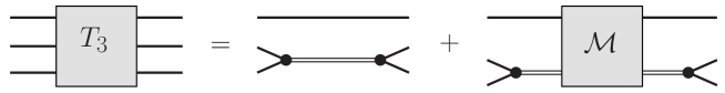
Figure 4: Expressing three-particle amplitude in terms of a particle-dimer amplitude. Summing up over all possible choices of spectator particles is implicit.

Up to this point, all expressions are manifestly Lorentz invariant, if the vector $v^{\mu}$ is also Lorentz-boosted along with other vectors. This means that, for instance, the particle-dimer amplitude ${\cal M}$, which implicitly depends on the choice of the quantization axis $v^{\mu}$, is invariant under arbitrary Lorentz boosts

$${\cal M}(\Lambda p;\Lambda q;\Lambda v)={\cal M}(p;q;v)\,.$$ (76)

In other words, after fixing $v^{\mu}$ in terms of the external momenta $p_{i},q_{j}$ (the most natural choice is, as already mentioned above, to choose $v^{\mu}$ along the total four-momentum $K^{\mu}$ of the three-particle system), the particle-dimer amplitude becomes manifestly Lorentz-invariant. Thus, the goal stated in the beginning has been achieved. We would like to stress here that this happens because the two-particle scattering amplitude after using the threshold expansion depends only on the pertinent Mandelstam variable $s$ for a given subsystem and does not depend on $v^{\mu}$. If it were not the case, one would be forced to fix the direction of the quantization axis for each subsystem separately, as well as for the whole system, and this cannot be done simultaneously. It is also clear that this approach will face difficulties in the study of the four-particle system, which contains different three-particle subsystems.

In conclusion, note that if the dimers with higher spin are taken into account, both the dimer propagator $S$ in Eq. (61) and the tree-level amplitude $T^{\sf tree}$ become matrices in the space of Lorentz indices, e.g., $S\to S_{\mu_{1}\ldots\mu_{\ell^{\prime}},\nu_{1}\ldots\nu_{\ell}}\doteq S_{n_{\ell^{\prime}}n_{\ell}}$ and $T^{\sf tree}\to T^{\sf tree}_{\mu_{1}\ldots\mu_{\ell^{\prime}},\nu_{1}\ldots\nu_{\ell}}\doteq T^{\sf tree}_{n_{\ell^{\prime}}n_{\ell}}$. All further steps can be performed in a direct analogy to the case of the scalar dimer. Namely, replacing $s_{p}$ by $\sigma_{q}^{2}$ and $s_{q}$ by $\sigma_{p}^{2}$ is straightforward. This leads to a system of equations (cf. with Eq. (70)):

$$\tilde{T}_{n_{\ell^{\prime}}n_{\ell}}(p,q) = \tilde{T}^{\sf tree}_{n_{\ell^{\prime}}n_{\ell}}(p,q)$$ (77)

$$+ \sum_{n_{\ell^{\prime\prime}}n_{\ell^{\prime\prime\prime}}}\int^{\Lambda_{v}}\frac{d^{3}k_{\perp}}{(2\pi)^{3}2w_{v}(k)}\,\tilde{T}^{\sf tree}_{n_{\ell^{\prime}}n_{\ell^{\prime\prime}}}(p,k)S_{n_{\ell^{\prime\prime}}n_{\ell^{\prime\prime\prime}}}((K-k)^{2})\tilde{T}_{n_{\ell^{\prime\prime\prime}}n_{\ell}}(k,q)\,.\quad\quad$$

Note that the matrix $S$ is diagonal in $\ell^{\prime},\ell$ in the infinite, but not in a finite volume. Furthermore,

$$\sum_{n_{\ell}}(\cdots)=\sum_{\ell=0}^{\ell_{max}}\sum_{\mu_{1},\cdots,\mu_{\ell}}(\cdots)\,.$$ (78)

Next, one may define:

$$\tilde{T}_{n_{\ell^{\prime}}n_{\ell}}(p,q) = f_{\ell^{\prime}}(\sigma_{p}^{2}){\cal M}_{n_{\ell^{\prime}}n_{\ell}}(p,q)f_{\ell}(\sigma_{q}^{2})\,,$$

$$\tilde{T}^{\sf tree}_{n_{\ell^{\prime}}n_{\ell}}(p,q) = f_{\ell^{\prime}}(\sigma_{p}^{2}){\cal Z}_{n_{\ell^{\prime}}n_{\ell}}(p,q)f_{\ell}(\sigma_{q}^{2})\,,$$

$$\tau_{n_{\ell^{\prime}}n_{\ell}}((K-k)^{2}) = f_{\ell^{\prime}}(\sigma_{k}^{2})S_{n_{\ell^{\prime}}n_{\ell}}((K-k)^{2})f_{\ell}(\sigma_{k}^{2})\,,$$

$$\sigma_{k}^{2} = (K-k)^{2}-4m^{2}\,.\quad$$ (79)

In the infinite volume, the matrix $\tau$ is also diagonal and contains the on-shell two-body partial-wave amplitudes.

The three-body amplitude is given by (cf. with Eq. (3.2)

$$T_{3}(p_{1},p_{2},p_{3};q_{1},q_{2},q_{3}) = T_{3}^{\sf disc}+T_{3}^{\sf conn}\,,$$

$$T_{3}^{\sf disc} = \sum_{i,j=1}^{3}(2\pi)^{3}\delta^{3}(p_{i\perp}-q_{j\perp})2w_{v}(p_{i})$$

$$\times \sum_{n_{\ell^{\prime}}n_{\ell}}Y_{n_{\ell^{\prime}}}(\bar{p}^{(i)})(\tau_{n_{\ell^{\prime}}n_{\ell}}((K-p_{i})^{2})Y_{n_{\ell}}(\bar{q}^{(j)})\,,$$

$$T_{3}^{\sf conn} = \sum_{i,j=1}^{3}\sum_{n_{\ell^{\prime\prime\prime}}n_{\ell^{\prime\prime}}n_{\ell^{\prime}}n_{\ell}}Y_{n_{\ell^{\prime\prime\prime}}}(\bar{p}^{(i)})\tau_{n_{\ell^{\prime\prime\prime}}n_{\ell^{\prime\prime}}}((K-p_{i})^{2}){\cal M}_{n_{\ell^{\prime\prime}}n_{\ell^{\prime}}}(p_{i},q_{j})$$ (80)

$$\times \tau_{n_{\ell^{\prime}}n_{\ell}}((K-q_{j})^{2})Y_{n_{\ell}}(\bar{q}^{(j)})\,.\quad\quad$$

The vectors $\bar{p}^{(i)},\bar{q}^{(j)}$ are defined through the Lorentz boost similar to one in Eq. (38). Namely, say, $p_{3}^{\mu}$ is a four-momentum of a spectator in the final state. Define now the boost $\Lambda^{\mu}_{\nu}$, which brings the total on-shell momentum of a pair $P_{12}^{\mu}=\tilde{p}_{1}^{\mu}+\tilde{p}_{2}^{\mu}$ parallel to the vector $v^{\mu}$. Then, $\bar{p}^{(3)\mu}=\frac{1}{2}\,\Lambda^{\mu}_{\nu}(\tilde{p}_{1}^{\nu}-\tilde{p}_{2}^{\nu})$. It can be also shown that $\bar{p}^{(i)\mu}=\bar{p}^{(i)\mu}_{\perp}=\bar{p}^{(i)\mu}-v^{\mu}(v\bar{p}^{(i)})$. The quantity $\bar{q}^{(j)}$ is defined similarly. Finally,

$$Y_{n_{\ell}}(\bar{p}^{(i)})\doteq Y_{\mu_{1},\cdots,\mu_{\ell}}(\bar{p}^{(i)})=\biggl{(}\frac{s}{4}-m^{2}\biggr{)}^{-\ell/2}\mathscr{Y}_{\mu_{1},\cdots,\mu_{\ell}}(\bar{p}^{(i)})\,,$$ (81)

where the tensor $\mathscr{Y}_{\mu_{1},\cdots,\mu_{\ell}}$ describes a particle with a spin $\ell$:

$$\mathscr{Y} = 1\,,$$

$$\mathscr{Y}_{\mu} = p^{\mu}\,,$$

$$\mathscr{Y}_{\mu\nu} = \frac{3}{2}\,p_{\mu}p_{\nu}-\frac{1}{2}\,(g_{\mu\nu}-v_{\mu}v_{\nu})p^{2}\,,$$

$$\cdots$$ (82)

and $s=(\tilde{p}_{1}+\tilde{p}_{2})^{2}$.

3.3 Quantization condition

In order to avoid the clutter of indices, we shall write down the quantization condition in case of the S-wave interactions only. We start by rewriting the Faddeev equation for the particle-dimer amplitude in a finite cubic box of size $L$ with periodic boundary conditions, where it takes the form:

$${\cal M}_{L}(p,q)={\cal Z}(p,q)+\frac{1}{L^{3}}\sum_{\bf k}\frac{1}{2w({\bf k})}\,\theta(\Lambda^{2}+m^{2}-(vk)^{2}){\cal Z}(p,k)\tau_{L}(K-k){\cal M}_{L}(k,q)\,.\quad\quad$$ (83)

Here, $k^{\mu}=(w({\bf k}),{\bf k})$ and $w({\bf k})=\sqrt{m^{2}+{\bf k}^{2}}$, and the summation is carried out over the discrete values ${\bf k}=\frac{2\pi}{L}\,{\bf n},~{}{\bf n}\in\mathbb{Z}^{3}$. Furthermore,

$$\tau_{L}(P)=\frac{16\pi\sqrt{s}}{p(s)\cot\delta_{0}(s)-\dfrac{2}{\sqrt{\pi}L\gamma}\,Z_{00}^{\bf d}(1;q_{0}^{2})}\,,$$ (84)

where $s=P^{2}$, $\gamma=\left(1-\dfrac{{\bf P}^{2}}{P_{0}^{2}}\right)^{-1/2}$, ${\bf d}=\dfrac{{\bf P}L}{2\pi}$, $q_{0}^{2}=\dfrac{L^{2}}{4\pi^{2}}\,\left(\dfrac{s}{4}-m^{2}\right)$, and

$$Z_{00}^{\bf d}(1;q_{0}^{2}) = \frac{1}{\sqrt{4\pi}}\sum_{{\bf r}\in P_{d}}\frac{1}{{\bf r}^{2}-q_{0}^{2}}\,,$$

$$P_{d} = \{{\bf r}=\mathbb{R}^{3}|r_{\parallel}=\gamma^{-1}\biggl{(}n_{\parallel}-\frac{1}{2}\,|{\bf d}|\biggr{)},\,{\bf r}_{\perp}={\bf n}_{\perp}\,,\,{\bf n}\in\mathbb{Z}^{3}\}\,.$$ (85)

A crucial point in the above expressions is that the two-body amplitude $\tau_{L}$ does not depend on $v^{\mu}$ even in a finite volume. In order to see this, note first that the expression $p(s)\cot\delta_{0}(s)$ is the same in the infinite and in finite volume and is $v^{\mu}$-independent. Furthermore, in the infinite volume, the loop is given by Eq. (10) and is explicitly Lorenz-invariant. In a finite volume, the three-momentum integral in this expression has to be replaced by a sum. The discretization is performed in the rest frame of a box. The result is given by the Lüscher zeta-function, which explicitly depends on the components of the vector $P^{\mu}$ (i.e., is not explicitly Lorentz-invariant) but not on $v^{\mu}$, which does not appear at any stage. A detailed derivation of Eq. (84) along these lines can be found in appendix A.

Next, the above expression is written down in the assumption that $s>0$. In case of $s<0$, the $\tau_{L}(P)$ is replaced by $\tau(P^{2})$ – as one knows, these two quantities below the two-particle threshold differ only by the exponentially suppressed terms. The latter is a perfectly well-defined Lorentz-invariant quantity and can be written down in terms of invariant kinematic variables, without performing any boost.

The quantization condition has the form $\det A=0$, where

$$A_{{\bf p}{\bf q}}=L^{3}2w({\bf p})\delta_{{\bf p}{\bf q}}\tau_{L}^{-1}(K-p)-{\cal Z}(p,q)\,,$$ (86)

and the momenta $p,q$ obey the condition $\Lambda^{2}+m^{2}-(vp)^{2}\geq 0$, $\Lambda^{2}+m^{2}-(vq)^{2}\geq 0$. The zeros of the determinant determine the finite-volume spectrum in an arbitrary reference frame.

As it is well known, the symmetries of a cubic box allow one to partially diagonalize the quantization condition. Below, we mainly follow the procedure described in Doring:2018xxx and generalize it to the case of the moving frame. In the CM frame, the rotational symmetry is reduced to the octahedral group $O_{h}$, containing 48 elements. In case of the moving frame, ${\bf K}\neq 0$, the symmetry is further reduced to different subgroups (little groups) of $O_{h}$, each element $g$ of which leaves the vector ${\bf d}=\dfrac{L{\bf K}}{2\pi}$ invariant: $g{\bf d}={\bf d}$. These symmetry groups and their irreps are described in Refs. Bernard:2008ax ; Gockeler:2012yj , where the matrices of the different irreps are explicitly given.

In order to carry out the diagonalization of the quantization condition into various irreps, one has first to introduce the notion of shells in the space of the discretized momenta ${\bf p}=\dfrac{2\pi}{L}\,{\bf n}$, ${\bf n}\in\mathbb{Z}^{3}$. In the CM frame, a shell is defined as a set of momenta that can be transformed into each other by the elements of the group $O_{h}$ Doring:2018xxx . All the elements of a given shell have the same length ${\bf n}^{2}$ but not all vectors with the same length belong to the same shell. In case of a moving frame, the shells are defined by two invariants ${\bf n}^{2}$, ${\bf n}{\bf d}$ instead of one.

Following Ref. Doring:2018xxx , we may project the driving term in the quantization condition onto various irreps $\mathit{\Gamma},\mathit{\Gamma}^{\prime}$:

$${\cal Z}_{\lambda\sigma,\rho\delta}^{\mathit{\Gamma}\mathit{\Gamma}^{\prime}}(r,s) = \sum_{g,g^{\prime}\in{\cal G}}(T^{\mathit{\Gamma}}_{\sigma\lambda}(g))^{*}{\cal Z}(g{\bf p}_{0}(r),g^{\prime}{\bf q}_{0}(s))T^{\mathit{\Gamma}^{\prime}}_{\delta\rho}(g^{\prime})$$ (87)

$$= \frac{G}{s_{\mathit{\Gamma}}}\,\delta_{\mathit{\Gamma}\mathit{\Gamma}^{\prime}}\delta_{\sigma\delta}\sum_{g\in{\cal G}}(T^{\mathit{\Gamma}}_{\rho\lambda}(g))^{*}{\cal Z}(g{\bf p}_{0}(r),{\bf q}_{0}(s))$$

$$\doteq \frac{G}{s_{\mathit{\Gamma}}}\,\delta_{\mathit{\Gamma}\mathit{\Gamma}^{\prime}}\delta_{\sigma\delta}{\cal Z}^{\mathit{\Gamma}}_{\lambda\rho}(r,s)\,.$$

Here, $r,s$ label various shells, ${\bf p}_{0}(r)$ and ${\bf q}_{0}(s)$ denote the pertinent reference momenta, and $T^{\mathit{\Gamma}}_{\sigma\lambda}(g)$ are the matrices of a given irrep of a group ${\cal G}$ (which coincides with the group $O_{h}$ or one of its little groups). Furthermore, $G$ is the number of the elements in this group, and $s_{\mathit{\Gamma}}$ is the dimension of the irrep $\mathit{\Gamma}$.

The quantization condition can be diagonalized into various irreps. It has the form $\det A^{\mathit{\Gamma}}=0$, where

$$A^{\mathit{\Gamma}}_{\rho\sigma}(r,s)=\delta_{rs}2w_{r}\delta_{\rho\sigma}\tau_{L}(s)^{-1}-\frac{\sqrt{\nu(r)\nu(s)}}{GL^{3}}\,{\cal Z}^{\mathit{\Gamma}}_{\sigma\rho}(r,s)\,,$$ (88)

where $\nu(s)$ denotes the multiplicity of the shell $s$, i.e., the number of the independent vectors in it, and $w_{r}=w({\bf p})$ with vector ${\bf p}$ belonging to the shell $r$. We have further used the fact that the quantity $\tau_{L}(K-k)$ is invariant under the group ${\cal G}$ and, hence, its projection onto an irrep $\mathit{\Gamma}$ produces Kronecker symbols only.

3.4 Comparison with the RFT approach

Below, we shall briefly compare the relativistic quantization condition, written down in the present paper, to the one known in the literature, see, for instance, Ref. Blanton:2019igq . Following the original derivation given in Refs. Hansen:2014eka ; Hansen:2015zga , one ends up with an equation that closely resembles Eq. (83) with the quantization axis chosen at $v^{\mu}=v_{0}^{\mu}$. It is easy to see that a sole manifestly non-invariant ingredient of this equation is the one-particle exchange part contained in ${\cal Z}$ (in Refs. Hansen:2014eka ; Hansen:2015zga ; Blanton:2019igq , this corresponds to the three-particle propagator $G$). In order to render the formalism Lorentz-invariant, the following approach was used. The three-particle propagator was replaced by

$$\frac{1}{2w({\bf l})}\,\frac{1}{w({\bf p})+w({\bf q})+w({\bf l})-K^{0}}$$ (89)

$$\to \frac{1}{2w({\bf l})}\,\frac{1}{w({\bf p})+w({\bf q})+w({\bf l})-K^{0}}+\frac{1}{2w({\bf l})}\,\frac{1}{w({\bf p})+w({\bf q})-w({\bf l})-K^{0}}$$

$$= \frac{1}{b^{2}-m^{2}}\,,$$

where $b^{\mu}=p^{\mu}+q^{\mu}-K^{\mu}$ and ${\bf l}={\bf K}-{\bf p}-{\bf q}$. It can be easily seen that the added piece is a low-energy polynomial and it can be removed by adjusting the renormalization prescription in the short-range three-particle interaction.

This approach is, however, problematic if applied to any formalism in which the cutoff on loop momenta can be raised arbitrarily high. The problem arises because the additional term did not emerge from a Feynman integral and thus does not have correct analytic properties. In particular, it can be seen that the contribution, coming from the integration region where both momenta ${\bf p}$ and ${\bf q}$ are large (of order of $m$), violates the unitarity in the infinite volume even in the low-energy region. This can be easily verified looking for the zeros of the expression $w({\bf p})+w({\bf q})-w({\bf l})-K^{0}$ for $K^{0}-3m=E\ll m$. In other words, the decoupling of the low- and high-momentum regimes, which is intimately related to the analytic properties of the amplitudes does not occur. In a finite volume, by the same token, it can be straightforwardly verified that the above modification of the three-particle propagator will result in a bunch of spurious subthreshold energy levels which have nothing to do with the real spectrum of a system in question.

All the above effects emerge, if the integration momentum exceeds some critical value, of order of the particle mass itself. In all analysis carried out within the RFT approach so far, the cutoff is kept lower than this value and, hence, the above-mentioned deficiency did not surface. However, this also means that the cutoff cannot be made arbitrary large in a framework with the modified three-particle propagator. On physical grounds, one may consider such a purely kinematic restriction on the cutoff rather counter-intuitive, since a cutoff is usually associated with the massive degrees of freedom that one intends to shield away. Moreover, one might be concerned of the fact that the maximal allowed value of the cutoff turns out to be of order of the particle mass. It is however likely that, by adapting the methodology introduced here, the cutoff in the RFT approach could be raised arbitrarily high while maintaining relativistic invariance, and in particular the Lorentz invariance of the three-particle amplitude $K_{\sf df,3}$.

In addition, we would like to mention that in the RFT approach, imposing a low cutoff can be also justified by the necessity of staying above the cross-channel cut in the two-body amplitude, as well as avoiding the pseudothreshold singularity in the Källen function (in the equal-mass case which is considered here, both, this singularity, as well as the beginning of the left-hand cut, are located at $s=0$, where $s$ is the pertinent Mandelstam variable in the two-body system). Analogous singularities could lead to $K_{\sf df,3}$ becoming complex-valued if the definition were modified by allowing for a higher cutoff function. In short, both the additional pole in the relativistic analog of the three-particle propagator $G$ and the cross-channel cut must be carefully considered in order to modify the cutoff function in the RFT method. This might be a formidable task in practice which the lower cutoff helps to avoid. The NREFT approach, in its turn, allows one to circumvent all these problems in a systematic fashion, since the two-body amplitudes constructed here possess the right-hand cut only, the three-body force, encoded in the effective couplings, is real by construction for all values of the cutoff function, and the three-particle propagator has only one pole. A simple physical explanation for this is that the antiparticle degrees of freedom, which are responsible for the additional (unwanted) singularities, are hidden in the couplings of the non-relativistic Lagrangian, both in the two- and three-particle sector. As one knows, this is justified only for momenta which are much smaller than the particle mass – for momenta of order of the mass both the two-body amplitude and the three-body potential are modified as compared to the relativistic theory. However, according to the decoupling theorem, the modification of the high-energy behavior of the amplitudes can be fully compensated at low energies by adjusting the renormalization prescription and thus does not lead to observable consequences. Loosely speaking, extending NREFT to describe amplitudes for momenta of order of the particle mass and beyond can be considered as a kind of a regularization, which consistently removes all singularities that emerge due to the presence of the antiparticles, and the cutoff is present solely to tame the ultraviolet behavior. Since all low-energy singularities are associated with particles only, the modified NREFT correctly reproduces the singularity structure of the amplitudes, and unitarity in the two- and three-particle sectors is obeyed at low energies. Furthermore, a finite-volume counterpart of this statement is that the quantization condition, based on the improved NREFT approach, neglects only exponentially suppressed volume effects at $mL\gg 1$, but makes no other approximations associated with the non-relativistic system. The choice to drop exponentially suppressed volume effects is common to all methods.

Last but not least, we would like to stress once more that the discussion of the distant singularities of different diagrams, which is given above, does not address the main question – namely, at which energies these singularities become physically important and cannot be brushed under the carpet anymore. This problem is common for all approaches since, as already mentioned, in order to derive the quantization condition, one is forced to restrict amplitudes on the mass shell and suppress explicit antiparticle degrees of freedom. At this moment, we do not have an answer to this very difficult question, which will also depend on a particular physical system considered. The perturbative studies might provide a clue on this issue. This, however forms a separate subject of investigations.

4 Exploring relativistic invariant quantization condition in a toy model

We have used the relativistic invariant quantization condition, derived within the NREFT approach in the previous section, for producing synthetic data within a toy model. The aim of this investigation is to verify that the spectrum, obtained in this manner, indeed obeys the requirements, imposed by the Lorentz invariance. In this section, we shall always used the choice for the vector $v^{\mu}$ parallel to the total four-momentum of the three-particle system $K^{\mu}$.

In the toy model, we consider the lowest-order S-wave interactions only, both in the two-particle as well as in the particle-dimer channels. This means that we have only two LECs: the non-derivative 4-particle coupling that is parameterized by the two-body scattering length $a$ and the dimensionless non-derivative particle-dimer coupling $H_{0}=H_{0}(\Lambda)$. The driving term in the Faddeev equation is written down as

$${\cal Z}(p,q)=\frac{1}{2w_{v}(K-p-q)(w_{v}(p)+w_{v}(q)+w_{v}(K-p-q)-vK-i\varepsilon)}+\frac{H_{0}(\Lambda)}{\Lambda^{2}}\,,$$ (90)

and the two-body propagator is given by

$$\tau(s)=\frac{16\pi\sqrt{s}}{-\frac{1}{a}-8\pi\sqrt{s}J(s)-ip(s)}\,.$$ (91)

In the non-relativistic limit, the first equation reduces to its non-relativistic counterpart displayed in Refs. Hammer:2017uqm ; Hammer:2017kms . Furthermore, the finite-volume modification of the second equation, which enters the quantization condition, is defined according to Eq. (84). In addition to $a,H_{0}$, there are two more parameters in the model: the mass of the particle $m$ and the cutoff $\Lambda$. In total, this yields three dimensionless parameters that describe the model completely – we measure all dimensionful parameters in the units of $m$ and assume $m=1$ in the following.

As the first quick check of our approach, we have calculated the spectrum of the so-called Efimov states in the infinite volume. An (infinite) tower of such shallow states, condensing towards the three-particle threshold, emerges in the non-relativistic theory in the unitary limit $a\to\infty$. Since in the vicinity of the threshold the particles should carry very low three-momenta, this non-relativistic result should be readily reproduced in the relativistic framework. Moreover, it is known that the binding energies of the neighboring Efimov states, $B_{n}=3m-E_{n}$, fulfill the relation:

$$\sqrt{B_{n}/B_{n+1}}=\exp\left(\pi/s_{0}\right)\approx 22.69\,,\quad\quad s_{0}=1.00624\,.$$ (92)

This scaling has to be reproduced by the relativistic approach, providing a check for the latter.

In the relativistic theory, we have fixed the remaining parameters in the unitary limit as $\Lambda=10^{4}$ and $H_{0}(\Lambda)=0$. The results, listed in Table 1, are completely in line with our expectations and confirm that our approach possesses a correct non-relativistic limit in the infinite volume.

$n$	$B_{n}$	$\sqrt{B_{n}/B_{n+1}}$
1	$3.323\,33\text{\times}{10}^{-1}\text{\,}$	21.93
2	$6.909\,73\text{\times}{10}^{-4}\text{\,}$	22.70
3	$1.341\,32\text{\times}{10}^{-6}\text{\,}$	22.69
4	$2.604\,32\text{\times}{10}^{-9}\text{\,}$	22.69
5	$5.056\,40\text{\times}{10}^{-12}\text{\,}$

Table 1: Binding energies of the five deepest states for $\Lambda=10^{4}$ and $H_{0}(\Lambda)=0$ in the unitary limit.

Next, the calculations in a finite volume are carried out where we go beyond the unitary limit. The scattering length and the cutoff in the toy model are chosen as $a=5$ and $\Lambda=3$, respectively (in the units of particle mass). For this value of the scattering length, a shallow dimer with the energy $E_{d}=1.94725$ emerges in the infinite volume and the particle-dimer threshold lies at $E_{1d}=2.94725$, close to the three-particle threshold. Furthermore, requiring the existence of a three-particle bound state at $E_{1}=2.6$ in the infinite volume fixes the value of the coupling $H_{0}=-0.1182689$. Another shallow three-particle bound state is found in the infinite volume at $E_{2}=2.94671$, very close to the particle-dimer-threshold. All energies are given in the rest frame.

Figure 5 shows the volume dependence of the energy spectrum in the rest frame and moving frames, $\mathbf{d}=(0,0,1)$, $\mathbf{d}=(0,1,1)$ and $\mathbf{d}=(1,1,1)$, obtained for the above choice of the parameters, above and below the three-particle threshold. The energy spectra are given in terms of $M^{\mathbf{d}}=M^{\mathbf{d}}(L)=\sqrt{K_{0}^{2}-(2\pi/L)^{2}\mathbf{d}^{2}}$, where $K_{0}=K_{0}(L)$ are the energies in a finite volume that fulfill the quantization condition. The lowest two levels in these figures, shown in blue and red, correspond to the deep and shallow bound states, respectively. As seen from these figures, the shallow bound state converges to its infinite-volume limit very slowly, as expected. Namely, for smaller $L$, the finite-volume energy is larger than the exact infinite-volume value. With the increase of $L$ it crosses the exact result and then approaches it from below very slowly, as $L\to\infty$. A similar behavior was observed in the non-relativistic case, see Ref. Doring:2018xxx , so the present result does not come as a surprise. As we shall see, such an irregular behavior complicates the numerical study of the large-$L$ limit of the shallow binding energy considerably, especially in the moving frames where the crossing emerges at larger values of $L$.

In order to check the relativistic invariance, we concentrate on the three-particle bound states. Indeed, it suffices to show that the quantity $M_{i}^{\mathbf{d}}-E_{i},~{}i=1,2$, where the quantity $M^{\mathbf{d}}$ was defined above, decreases exponentially for large values of $L$. In this case, it can be seen that the one-particle states, obtained by solving the quantization condition, obey the relativistic dispersion law up to the exponentially suppressed corrections. This is exactly the result one is looking for.

The result of the calculations is shown in Fig. 6. In case of the deep state, everything works fine. The logarithmic plot for the difference is almost a perfect straight line that is compatible with an exponential decrease $\sim\exp(-\kappa_{\sf deep}L)$ and $\kappa_{\sf deep}\simeq 0.7$ for all frames. The situation with the shallow state is different. As mentioned above, the finite- and infinite-volume energies coincide at some $L$. This is manifested by the dips in the curves presented on the right panel. After the dip, it takes very large values of $L$ for the curves to stabilize and show a linear behavior. In case of the rest frame, the curve becomes almost linear after $L\simeq 12-15$, see Fig. 7 (here, large values of $L$ are shown). This behavior is consistent with the exponential decrease $\sim\exp(-\kappa_{\sf shallow}L)$ and $\kappa_{\sf shallow}\simeq 0.11,0.03$ for the frames $\mathbf{d}=(0,0,0),(0,0,1)$. Note that the arguments of the exponent can be different in different frames, because the Lorentz symmetry is broken in a finite volume. Furthermore, the dips in the $\mathbf{d}=(0,1,1),(1,1,1)$ frames occur at much larger values of $L$. Since carrying out calculations on such large grids is very time-consuming, we display here the results for two reference frames only. Note also that here we did not make an attempt to predict the values of $\kappa$ in different frames. Albeit such a theoretical prediction is possible in principle, it is not relevant in the context of the problem considered in the present paper.

To summarize, in this section it was explicitly checked that the three-particle bound states, obtained from the solution of the quantization condition, obey the relativistic dispersion law up to the exponentially suppressed corrections. Recall now that the analysis of the lattice data in the three-particle sector proceeds in two steps. At the first step, the quantities having a short-range nature (like the coupling $H_{0}$) are extracted from data. These quantities, like the bound-state energies, can receive only exponentially suppressed corrections and, hence, up to such corrections, one may use the same values of these quantities in the fit of data coming from different moving frames. This is exactly the manifestation of the Lorentz-invariance in a finite box. At the end, as usual, one uses an explicitly Lorentz-invariant infinite-volume formalism to express physical observables through the couplings $H_{0},\ldots$, extracted from data.

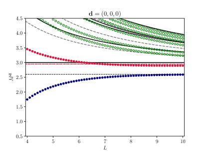
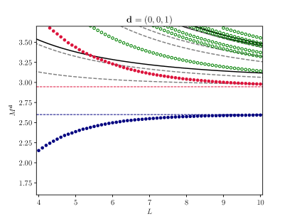
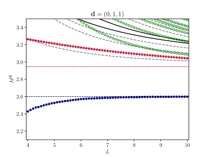
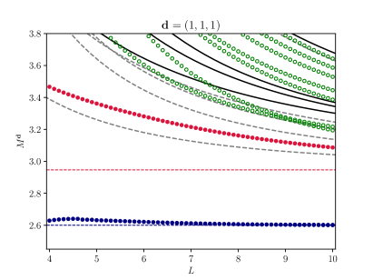
Figure 5: Dependence of the energy levels on the box size $L$ in the rest frame and moving frames. Blue and red dotted curves correspond to the energy of the deep and shallow bound states, respectively, and the green dotted curves denote the so-called scattering states. The solid black lines and the gray dashed lines represent the energies of three free particles and a free particle-dimer system in a finite volume, respectively. Horizontal blue and red dashed lines indicate the energies of the infinite-volume deep and shallow bound states. One observes an avoided level crossing (related, presumably, to the crossing of the free particle-dimer levels) in the frame ${\bf d}=(1,1,1)$ but not in the other frames. Thus, this is a purely kinematic effect.

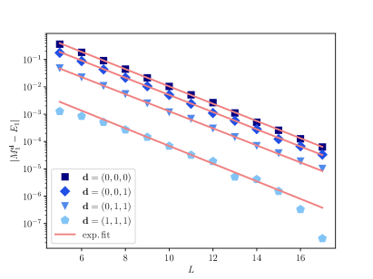
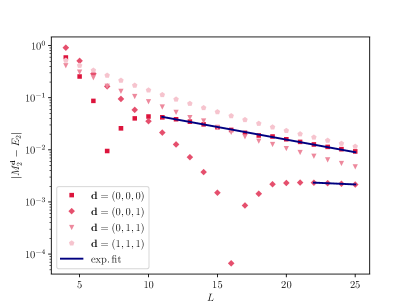
Figure 6: The difference between the finite- and infinite-volume binding energies for the deep (left panel) and shallow (right panel) bound states. Note that for a better visibility, we have divided the energy shift of the deep bound state, corresponding to ${\bf d}=(1,1,1)$, by a factor $25$. Otherwise, the data for ${\bf d}=(0,1,1)$ and ${\bf d}=(1,1,1)$ would nearly overlap.

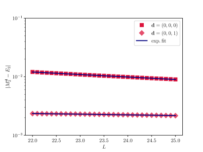
Figure 7: The differences between the finite- and infinite-volume binding energies for the shallow bound state at larger values of $L$. The straight lines show the results of the exponential fit.

5 Conclusions

• In this paper, we have proposed a manifestly relativistically invariant formulation of the three-particle quantization condition within the NREFT approach. It is shown that the higher partial waves can be consistently included in the formulation. The suggested framework can be readily used for the global analysis of lattice spectra, measured in different moving frames. This was already done in case of RFT and FVU approaches.

• The method, described in this paper, is very well known for decades in the literature and is based on the formulation of the three-particle problem with an arbitrary chosen quantization axis defined by a unit timelike vector $v^{\mu}$ (see, e.g., Ref. Kadyshevsky:1967rs ). At the end, the vector $v^{\mu}$ is fixed in terms of the external momenta that renders the framework manifestly invariant. The most obvious choice is to take that vector parallel to the total three-momentum of the system, and we stick to this choice. It should be also mentioned that this construction relies on the fact that the scattering amplitudes in the various two-particle subsystems, which are calculated by using the dimensional regularization and threshold expansion, are explicitly invariant (i.e., do not depend in $v^{\mu}$) even before fixing it in terms of the external momenta. For instance, this property is lost if the cutoff regularization is used for the two-particle subsystems as well. By the same token, a similar approach will encounter difficulties when applied to the four-particle problem, which features three-particle subsystems. This issue, however, lies beyond the scope of the present paper.

• The choice of the quantization axis along an arbitrary timelike vector $v^{\mu}$ does not affect the analytic properties of the non-relativistic amplitudes. Hence, there is no violation of unitarity in this approach, and spurious poles do not emerge from the quantization condition.

• The proposed framework has been tested within a toy model. It has been shown that the three-particle bound spectrum is explicitly Lorentz-invariant, i.e., the finite-volume corrections to the three-particle binding energies, obtained in different moving frames, are exponentially suppressed in $L$.

• In our opinion, it will be rather straightforward to adapt the proposed method for other approaches used in the literature (RFT and FVU). An alternative method, proposed within the RFT approach, can also be used. Within this method, a cutoff on the three-momenta cannot be moved beyond some maximal value of order of a particle mass, albeit all results obtained by using the cutoffs less than this value are still valid.

Appendix A Two-body amplitude in a finite volume

This appendix proves the $v^{\mu}$-independence of the finite volume two-body amplitude by providing an explicit derivation of Eq. (84). Calculating the two-particle scattering amplitude in a finite volume amounts to replacing the loop integral $I$ defined in Eq. (7) by its finite volume counterpart $I_{L}$.

$$I_{L}=\frac{1}{L^{3}}\sum_{{\bf k}}\int\frac{dk_{0}}{2\pi i}\,\frac{1}{2w_{v}(k)(w_{v}(k)-vk-i\varepsilon)}\,\frac{1}{2w_{v}(P-k)(w_{v}(P-k)-v(P-k)-i\varepsilon)}\,.$$

At this stage, one uses Eq. (8). Adding and subtracting the real part of the same quantity, calculated in the infinite volume, one gets:

$$I_{L} = \text{Re}(I(s))+\left[\frac{1}{L^{3}}\sum_{{\bf k}}-\mathcal{P}\int\frac{d^{3}{\bf k}}{(2\pi)^{3}}\right]$$ (94)

$$\times \int\frac{dk_{0}}{2\pi i}\,\biggl{\{}\frac{1}{(m^{2}-k^{2}-i\varepsilon)(m^{2}-(P-k)^{2}-i\varepsilon)}+\Delta\biggr{\}}\,.$$

Here, the quantity $I(s)$ and the real part thereof are given by Eqs. (10)-(12). Furthermore, the quantity $\Delta$ is equal to

$$\Delta = \frac{1}{m^{2}-k^{2}-i\varepsilon}\,\frac{1}{2w_{v}(P-k)(w_{v}(P-k)+v(P-k)-i\varepsilon)}$$ (95)

$$+ \frac{1}{m^{2}-(P-k)^{2}-i\varepsilon}\,\frac{1}{2w_{v}(k)(w_{v}(k)+vk-i\varepsilon)}$$

$$+ \frac{1}{2w_{v}(k)(w_{v}(k)+vk-i\varepsilon)}\,\frac{1}{2w_{v}(P-k)(w_{v}(P-k)+v(P-k)-i\varepsilon)}\,.$$

The energy denominators in the above expression can be expanded, according to Eq. (9). The last term turns then into a low-energy polynomial. The first two terms contain a single low-energy pole in $k^{0}$ each, at $k^{0}=\sqrt{m^{2}+{\bf k}^{2}}$ and $k^{0}=P^{0}-\sqrt{m^{2}+({\bf P}-{\bf k})^{2}}$, respectively. Integrating over $k^{0}$ leads to a low-energy polynomial again. In the infinite volume, such low-energy polynomials do not contribute to the integrals over spatial components of momenta in dimensional regularization. In a finite volume, the sum minus integral over spatial components of momenta gives a contribution that is exponentially suppressed in the box size $L$. Neglecting these exponential terms, it is seen that the contribution from $\Delta$ vanishes completely, and one can finally write:

$$I_{L}=J(s)+\left[\frac{1}{L^{3}}\sum_{{\bf k}}-\mathcal{P}\int\frac{d^{3}{\bf k}}{(2\pi)^{3}}\right]\int\frac{dk_{0}}{2\pi i}\,\frac{1}{(m^{2}-k^{2}-i\varepsilon)(m^{2}-(P-k)^{2}-i\varepsilon)}\,.$$ (96)

The explicit $v^{\mu}$-dependence disappears already at this stage. The subsequent steps are pretty standard. Evaluating the integral over $k^{0}$ gives:

$$I_{L} = J(s)+\left[\frac{1}{L^{3}}\sum_{{\bf k}}-\mathcal{P}\int\frac{d^{3}k}{(2\pi)^{3}}\right]\frac{1}{2w({\bf k})w({\bf P-k})}\frac{w({\bf k})+w({\bf P-k})}{(w({\bf k})+w({\bf P-k}))^{2}-P_{0}^{2}}$$ (97)

$$= J(s)+\left[\frac{1}{L^{3}}\sum_{{\bf k}}-\mathcal{P}\int\frac{d^{3}k}{(2\pi)^{3}}\right]\frac{1}{4w({\bf k})w({\bf P-k})(w({\bf k})+w({\bf P-k})-P_{0})}$$

$$= J(s)+\frac{1}{4\pi^{3/2}L\gamma\sqrt{s}}Z_{00}^{\bf d}(1;q_{0}^{2})\,.$$

The integrands in the first and second line differ by $\bigl{[}4w({\bf k})w({\bf P-k})(w({\bf k})+w({\bf P-k})+P_{0})\bigr{]}^{-1}$. Since this is a low-energy polynomial in the three-momenta, it gives rise only to the exponentially suppressed corrections. Finally, following Ref. Bernard:2008ax , the sum minus integral in the fourth line can be expressed through the Lüscher zeta-function, as defined in Eq. (3.3).

Noting that the tree-level amplitude is the same in the infinite and finite volume, the resulting two-body S-wave scattering amplitude in a finite volume reads as

$$\tau_{L}(P)=\frac{1}{(T^{\sf S-wave}_{\sf tree})^{-1}-\frac{1}{2}\,I_{L}(P)}=\frac{16\pi\sqrt{s}}{p(s)\cot\delta_{0}(s)-\dfrac{2}{\sqrt{\pi}L\gamma}\,Z_{00}^{\bf d}(1;q_{0}^{2})}\,,$$ (98)

where $p(s)\cot\delta_{0}(s)$ is given by Eq. (21).

References

- (1) K. Polejaeva and A. Rusetsky, “Three particles in a finite volume,” Eur. Phys. J. A 48 (2012) 67 [arXiv:1203.1241 [hep-lat]].
- (2) M. T. Hansen and S. R. Sharpe, “Relativistic, model-independent, three-particle quantization condition,” Phys. Rev. D 90 (2014) 116003 [arXiv:1408.5933 [hep-lat]].
- (3) M. T. Hansen and S. R. Sharpe, “Expressing the three-particle finite-volume spectrum in terms of the three-to-three scattering amplitude,” Phys. Rev. D 92 (2015) 114509 [arXiv:1504.04248 [hep-lat]].
- (4) H. W. Hammer, J. Y. Pang and A. Rusetsky, “Three-particle quantization condition in a finite volume: 1. The role of the three-particle force,” JHEP 09 (2017) 109 [arXiv:1706.07700 [hep-lat]].
- (5) H. W. Hammer, J. Y. Pang and A. Rusetsky, “Three particle quantization condition in a finite volume: 2. general formalism and the analysis of data,” JHEP 10 (2017) 115 [arXiv:1707.02176 [hep-lat]].
- (6) M. Mai and M. Döring, “Three-body Unitarity in the Finite Volume,” Eur. Phys. J. A 53 (2017) 240 [arXiv:1709.08222 [hep-lat]].
- (7) M. Mai and M. Döring, “Finite-Volume Spectrum of and Systems,” Phys. Rev. Lett. 122 (2019) 062503 [arXiv:1807.04746 [hep-lat]].
- (8) U.-G. Meißner, G. Rios and A. Rusetsky, “Spectrum of three-body bound states in a finite volume,” Phys. Rev. Lett. 114 (2015) 091602, Erratum: [Phys. Rev. Lett. 117 (2016) 069902] [arXiv:1412.4969 [hep-lat]].
- (9) M. Jansen, H. W. Hammer and Y. Jia, “Finite volume corrections to the binding energy of the X(3872),” Phys. Rev. D 92 (2015) 114031 [arXiv:1505.04099 [hep-ph]].
- (10) M. T. Hansen and S. R. Sharpe, “Perturbative results for two and three particle threshold energies in finite volume,” Phys. Rev. D 93 (2016) 014506 [arXiv:1509.07929 [hep-lat]].
- (11) M. T. Hansen and S. R. Sharpe, “Threshold expansion of the three-particle quantization condition,” Phys. Rev. D 93 (2016) 096006 [arXiv:1602.00324 [hep-lat]].
- (12) P. Guo, “One spatial dimensional finite volume three-body interaction for a short-range potential,” Phys. Rev. D 95 (2017) 054508 [arXiv:1607.03184 [hep-lat]].
- (13) S. König and D. Lee, “Volume Dependence of N-Body Bound States,” Phys. Lett. B 779 (2018) 9 [arXiv:1701.00279 [hep-lat]].
- (14) R. A. Briceño, M. T. Hansen and S. R. Sharpe, “Relating the finite-volume spectrum and the two-and-three-particle matrix for relativistic systems of identical scalar particles,” Phys. Rev. D 95 (2017) 074510 [arXiv:1701.07465 [hep-lat]].
- (15) S. R. Sharpe, “Testing the threshold expansion for three-particle energies at fourth order in theory,” Phys. Rev. D 96 (2017) 054515 [arXiv:1707.04279 [hep-lat]].
- (16) P. Guo and V. Gasparian, “Numerical approach for finite volume three-body interaction,” Phys. Rev. D 97 (2018) 014504 [arXiv:1709.08255 [hep-lat]].
- (17) P. Guo and V. Gasparian, “An solvable three-body model in finite volume,” Phys. Lett. B 774 (2017) 441 [arXiv:1701.00438 [hep-lat]].
- (18) Y. Meng, C. Liu, U.-G. Meißner and A. Rusetsky, “Three-particle bound states in a finite volume: unequal masses and higher partial waves,” Phys. Rev. D 98 (2018) 014508 [arXiv:1712.08464 [hep-lat]].
- (19) P. Guo, M. Döring and A. P. Szczepaniak, “Variational approach to -body interactions in finite volume,” Phys. Rev. D 98 (2018) 094502 [arXiv:1810.01261 [hep-lat]].
- (20) P. Guo and T. Morris, “Multiple-particle interaction in -dimensional lattice model,” Phys. Rev. D 99 (2019) 014501 [arXiv:1808.07397 [hep-lat]].
- (21) P. Klos, S. König, H. W. Hammer, J. E. Lynn and A. Schwenk, “Signatures of few-body resonances in finite volume,” Phys. Rev. C 98 (2018) 034004 [arXiv:1805.02029 [nucl-th]].
- (22) R. A. Briceño, M. T. Hansen and S. R. Sharpe, “Numerical study of the relativistic three-body quantization condition in the isotropic approximation,” Phys. Rev. D 98 (2018) 014506 [arXiv:1803.04169 [hep-lat]].
- (23) R. A. Briceño, M. T. Hansen and S. R. Sharpe, “Three-particle systems with resonant subprocesses in a finite volume,” Phys. Rev. D 99 (2019) 014516 [arXiv:1810.01429 [hep-lat]].
- (24) M. Döring, H. W. Hammer, M. Mai, J. Y. Pang, A. Rusetsky and J. Wu, “Three-body spectrum in a finite volume: the role of cubic symmetry,” Phys. Rev. D 97 (2018) 114508 [arXiv:1802.03362 [hep-lat]].
- (25) A. W. Jackura, S. M. Dawid, C. Fernández-Ramírez, V. Mathieu, M. Mikhasenko, A. Pilloni, S. R. Sharpe and A. P. Szczepaniak, “Equivalence of three-particle scattering formalisms,” Phys. Rev. D 100 (2019) 034508 [arXiv:1905.12007 [hep-ph]].
- (26) M. Mai, M. Döring, C. Culver and A. Alexandru, “Three-body unitarity versus finite-volume spectrum from lattice QCD,” Phys. Rev. D 101 (2020) 054510 [arXiv:1909.05749 [hep-lat]].
- (27) T. D. Blanton, F. Romero-López and S. R. Sharpe, “Implementing the three-particle quantization condition including higher partial waves,” JHEP 03 (2019) 106 [arXiv:1901.07095 [hep-lat]].
- (28) R. A. Briceño, M. T. Hansen, S. R. Sharpe and A. P. Szczepaniak, “Unitarity of the infinite-volume three-particle scattering amplitude arising from a finite-volume formalism,” Phys. Rev. D 100 (2019) 054508 [arXiv:1905.11188 [hep-lat]].
- (29) F. Romero-López, S. R. Sharpe, T. D. Blanton, R. A. Briceño and M. T. Hansen, “Numerical exploration of three relativistic particles in a finite volume including two-particle resonances and bound states,” JHEP 10 (2019) 007 [arXiv:1908.02411 [hep-lat]].
- (30) J. Y. Pang, J. J. Wu, H. W. Hammer, U.-G. Meißner and A. Rusetsky, “Energy shift of the three-particle system in a finite volume,” Phys. Rev. D 99 (2019) 074513 [arXiv:1902.01111 [hep-lat]].
- (31) P. Guo and M. Döring, “Lattice model of heavy-light three-body system,” Phys. Rev. D 101 (2020) 034501 [arXiv:1910.08624 [hep-lat]].
- (32) J. Y. Pang, J. J. Wu and L. S. Geng, “ system in finite volume,” Phys. Rev. D 102 (2020) 114515 [arXiv:2008.13014 [hep-lat]].
- (33) M. T. Hansen, F. Romero-López and S. R. Sharpe, “Generalizing the relativistic quantization condition to include all three-pion isospin channels,” JHEP 07 (2020) 047 [arXiv:2003.10974 [hep-lat]].
- (34) P. Guo, “Modeling few-body resonances in finite volume,” Phys. Rev. D 102 (2020) 054514 [arXiv:2007.12790 [hep-lat]].
- (35) S. König, “Few-body bound states and resonances in finite volume,” Few Body Syst. 61 (2020) 20 [arXiv:2005.01478 [hep-lat]].
- (36) T. D. Blanton and S. R. Sharpe, “Alternative derivation of the relativistic three-particle quantization condition,” Phys. Rev. D 102 (2020) 054520 [arXiv:2007.16188 [hep-lat]].
- (37) T. D. Blanton and S. R. Sharpe, “Relativistic three-particle quantization condition for nondegenerate scalars,” [arXiv:2011.05520 [hep-lat]].
- (38) R. Brett, C. Culver, M. Mai, A. Alexandru, M. Döring and F. X. Lee, “Three-body interactions from the finite-volume QCD spectrum,” [arXiv:2101.06144 [hep-lat]].
- (39) T. D. Blanton and S. R. Sharpe, “Three-particle finite-volume formalism for and related systems,” [arXiv:2105.12094 [hep-lat]].
- (40) S. Kreuzer and H.-W. Hammer, “The Triton in a finite volume,” Phys. Lett. B 694 (2011) 424 [arXiv:1008.4499 [hep-lat]].
- (41) S. Kreuzer and H.-W. Hammer, “On the modification of the Efimov spectrum in a finite cubic box,” Eur. Phys. J. A 43 (2010) 229 [arXiv:0910.2191 [nucl-th]].
- (42) S. Kreuzer and H.-W. Hammer, “Efimov physics in a finite volume,” Phys. Lett. B 673 (2009) 260 [arXiv:0811.0159 [nucl-th]].
- (43) S. Kreuzer and H.-W. Grießhammer, “Three particles in a finite volume: The breakdown of spherical symmetry,” Eur. Phys. J. A 48 (2012) 93 [arXiv:1205.0277 [nucl-th]].
- (44) R. A. Briceno and Z. Davoudi, “Three-particle scattering amplitudes from a finite volume formalism,” Phys. Rev. D 87 (2013) 094507 [arXiv:1212.3398 [hep-lat]].
- (45) T. D. Blanton and S. R. Sharpe, “Equivalence of relativistic three-particle quantization conditions,” Phys. Rev. D 102 (2020) 054515 [arXiv:2007.16190 [hep-lat]].
- (46) T. D. Lee, K. Huang and C. N. Yang, “Eigenvalues and Eigenfunctions of a Bose System of Hard Spheres and Its Low-Temperature Properties,” Phys. Rev. 106 (1957) 1135.
- (47) K. Huang and C. N. Yang, “Quantum-mechanical many-body problem with hard-sphere interaction,” Phys. Rev. 105 (1957) 767.
- (48) T. T. Wu, “Ground State of a Bose System of Hard Spheres,” Phys. Rev. 115 (1959) 1390.
- (49) S. Tan, “Three-boson problem at low energy and implications for dilute Bose-Einstein condensates,” Phys. Rev. A 78 (2008) 013636 [arXiv:0709.2530 [cond-mat.stat-mech]].
- (50) S. R. Beane, W. Detmold and M. J. Savage, “-Boson Energies at Finite Volume and Three-Boson Interactions,” Phys. Rev. D 76 (2007) 074507 [arXiv:0707.1670 [hep-lat]].
- (51) W. Detmold and M. J. Savage, “The Energy of Identical Bosons in a Finite Volume at ,” Phys. Rev. D 77 (2008) 057502 [arXiv:0801.0763 [hep-lat]].
- (52) S. R. Beane, W. Detmold, R. Horsley, M. Illa, M. Jafry, D. J. Murphy, Y. Nakamura, H. Perlt, P. E. L. Rakow and G. Schierholz, et al. “Charged multi-hadron systems in lattice QCD+QED,” Phys. Rev. D 103 (2021) 054504 [arXiv:2003.12130 [hep-lat]].
- (53) F. Romero-López, A. Rusetsky, N. Schlage and C. Urbach, “Relativistic -particle energy shift in finite volume,” JHEP 60 (2021) 60 [arXiv:2010.11715 [hep-lat]].
- (54) F. Müller, T. Yu and A. Rusetsky, “Finite-volume energy shift of the three-pion ground state,” Phys. Rev. D 103 (2021) 054506 [arXiv:2011.14178 [hep-lat]].
- (55) S. R. Beane, W. Detmold, T. C. Luu, K. Orginos, M. J. Savage and A. Torok, “Multi-Pion Systems in Lattice QCD and the Three-Pion Interaction,” Phys. Rev. Lett. 100 (2008) 082004 [arXiv:0710.1827 [hep-lat]].
- (56) W. Detmold, M. J. Savage, A. Torok, S. R. Beane, T. C. Luu, K. Orginos and A. Parreno, “Multi-Pion States in Lattice QCD and the Charged-Pion Condensate,” Phys. Rev. D 78 (2008) 014507 [arXiv:0803.2728 [hep-lat]].
- (57) W. Detmold, K. Orginos, M. J. Savage and A. Walker-Loud, “Kaon Condensation with Lattice QCD,” Phys. Rev. D 78 (2008) 054514 [arXiv:0807.1856 [hep-lat]].
- (58) T. D. Blanton, F. Romero-López and S. R. Sharpe, “ Three-Pion Scattering Amplitude from Lattice QCD,” Phys. Rev. Lett. 124 (2020) 032001 [arXiv:1909.02973 [hep-lat]].
- (59) B. Hörz and A. Hanlon, “Two- and three-pion finite-volume spectra at maximal isospin from lattice QCD,” Phys. Rev. Lett. 123 (2019) 142002 [arXiv:1905.04277 [hep-lat]].
- (60) C. Culver, M. Mai, R. Brett, A. Alexandru and M. Döring, “Three pion spectrum in the channel from lattice QCD,” Phys. Rev. D 101 (2020) 114507 [arXiv:1911.09047 [hep-lat]].
- (61) M. Fischer, B. Kostrzewa, L. Liu, F. Romero-López, M. Ueding and C. Urbach, “Scattering of two and three physical pions at maximal isospin from lattice QCD,” Eur. Phys. J. C 81 (2021) 436 [arXiv:2008.03035 [hep-lat]].
- (62) M. T. Hansen, R. A. Briceño, R. G. Edwards, C. E. Thomas and D. J. Wilson, “The energy-dependent scattering amplitude from QCD,” Phys. Rev. Lett. 126 (2021) 012001 [arXiv:2009.04931 [hep-lat]].
- (63) A. Alexandru, R. Brett, C. Culver, M. Döring, D. Guo, F. X. Lee and M. Mai, “Finite-volume energy spectrum of the system,” Phys. Rev. D 102 (2020) 114523 [arXiv:2009.12358 [hep-lat]].
- (64) F. Romero-López, A. Rusetsky and C. Urbach, “Two- and three-body interactions in theory from lattice simulations,” Eur. Phys. J. C 78 (2018) 846 [arXiv:1806.02367 [hep-lat]].
- (65) T. D. Blanton, A. D. Hanlon, B. Hörz, C. Morningstar, F. Romero-López and S. R. Sharpe, “Interactions of two and three mesons including higher partial waves from lattice QCD,” [arXiv:2106.05590 [hep-lat]].
- (66) L. Lellouch and M. Lüscher, “Weak transition matrix elements from finite volume correlation functions,” Commun. Math. Phys. 219 (2001) 31 [arXiv:hep-lat/0003023 [hep-lat]].
- (67) F. Müller and A. Rusetsky, “On the three-particle analog of the Lellouch-Lüscher formula,” JHEP 03 (2021) 152 [arXiv:2012.13957 [hep-lat]].
- (68) M. T. Hansen, F. Romero-López and S. R. Sharpe, “Decay amplitudes to three hadrons from finite-volume matrix elements,” JHEP 04 (2021) 113 [arXiv:2101.10246 [hep-lat]].
- (69) M. T. Hansen and S. R. Sharpe, “Lattice QCD and Three-particle Decays of Resonances,” Ann. Rev. Nucl. Part. Sci. 69 (2019) 65 [arXiv:1901.00483 [hep-lat]].
- (70) M. Mai, M. Döring and A. Rusetsky, “Multi-particle systems on the lattice and chiral extrapolations: a brief review,” [arXiv:2103.00577 [hep-lat]].
- (71) M. Mai, B. Hu, M. Döring, A. Pilloni and A. Szczepaniak, “Three-body Unitarity with Isobars Revisited,” Eur. Phys. J. A 53 (2017) 177 [arXiv:1706.06118 [nucl-th]].
- (72) G. Colangelo, J. Gasser, B. Kubis and A. Rusetsky, “Cusps in decays,” Phys. Lett. B 638 (2006) 187 [arXiv:hep-ph/0604084 [hep-ph]].
- (73) J. Gasser, B. Kubis and A. Rusetsky, “Cusps in decays: a theoretical framework,” Nucl. Phys. B 850 (2011) 96 [arXiv:1103.4273 [hep-ph]].
- (74) M. Bissegger, A. Fuhrer, J. Gasser, B. Kubis and A. Rusetsky, “Radiative corrections in decays,” Nucl. Phys. B 806 (2009) 178 [arXiv:0807.0515 [hep-ph]].
- (75) M. Bissegger, A. Fuhrer, J. Gasser, B. Kubis and A. Rusetsky, “Cusps in decays,” Phys. Lett. B 659 (2008) 576 [arXiv:0710.4456 [hep-ph]].
- (76) C. O. Gullstrom, A. Kupsc and A. Rusetsky, “Predictions for the cusp in decay,” Phys. Rev. C 79 (2009) 028201 [arXiv:0812.2371 [hep-ph]].
- (77) M. Beneke and V. A. Smirnov, “Asymptotic expansion of Feynman integrals near threshold,” Nucl. Phys. B 522 (1998) 321 [arXiv:hep-ph/9711391 [hep-ph]].
- (78) J. J. Wu, T. S. H. Lee, D. B. Leinweber, A. W. Thomas and R. D. Young, JPS Conf. Proc. 10 (2016) 062002 [arXiv:1512.02771 [hep-lat]].
- (79) Y. Li, J. j. Wu, D. B. Leinweber and A. W. Thomas, “Hamiltonian effective field theory in elongated or moving finite volume,” Phys. Rev. D 103 (2021) 094518 [arXiv:2103.12260 [hep-lat]].
- (80) Y. Li, J. J. Wu, R. D. Young and T. S. H. Lee, in preparation.
- (81) P. F. Bedaque, G. Rupak, H. W. Griesshammer and H. W. Hammer, “Low-energy expansion in the three-body system to all orders and the triton channel,” Nucl. Phys. A 714 (2003) 589 [arXiv:nucl-th/0207034 [nucl-th]].
- (82) V. Bernard, M. Lage, U.-G. Meißner and A. Rusetsky, “Resonance properties from the finite-volume energy spectrum,” JHEP 08 (2008) 024 [arXiv:0806.4495 [hep-lat]].
- (83) M. Gockeler, R. Horsley, M. Lage, U.-G. Meißner, P. E. L. Rakow, A. Rusetsky, G. Schierholz and J. M. Zanotti, “Scattering phases for meson and baryon resonances on general moving-frame lattices,” Phys. Rev. D 86 (2012) 094513 [arXiv:1206.4141 [hep-lat]].
- (84) V. G. Kadyshevsky, “Quasipotential type equation for the relativistic scattering amplitude,” Nucl. Phys. B 6 (1968) 125.
- (85) G. Leibbrandt and J. Williams, “Split dimensional regularization for the Coulomb gauge,” Nucl. Phys. B 475 (1996) 469. [arXiv:hep-th/9601046 [hep-th]].