Attention-Free Keyword Spotting

Abstract

Till now, attention-based models have been used with great success in the keyword spotting problem domain. However, in light of recent advances in deep learning, the question arises whether self-attention is truly irreplaceable for recognizing speech keywords. We thus explore the usage of gated MLPs—previously shown to be alternatives to transformers in vision tasks—for the keyword spotting task. We provide a family of highly efficient MLP-based models for keyword spotting, with less than 0.5 million parameters. We show that our approach achieves competitive performance on Google Speech Commands V2-12 and V2-35 benchmarks with much fewer parameters than self-attention-based methods.

1 Introduction

Transformers (Vaswani et al., 2017) have shown remarkable success in Computer Vision tasks with the advent of the Vision Transformer (ViT) (Dosovitskiy et al., 2020). They have lately been studied in the field of keyword spotting (KWS). Several works (Berg et al., 2021; Gong et al., 2021) have obtained exceptional results with ViT-like approaches on KWS.

Recent research (Tolstikhin et al., 2021; Liu et al., 2021; Melas-Kyriazi, 2021; Touvron et al., 2021a) shows that a core component of Transformers, self-attention, may not be necessary for achieving good performance in vision and language tasks. This finding necessitates a study on whether MLPs can be an alternative to self-attention, which has been a main focus of several state-of-the-art methods for the KWS problem. Our contributions can be summarized as follows:

1. We introduce the Keyword-MLP (KW-MLP), a memory-efficient, attention-free alternative to the Keyword Transformer (KWT) (Berg et al., 2021). It achieves 97.63% and 97.56% accuracy on the Google Speech Commands V2-12 and V2-35 benchmarks (Warden, 2018) respectively—showing comparable performance to the KWT, while having much fewer parameters.

2. We distill smaller and shallower versions of KW-MLP, with the smallest having only 0.213 million parameters, and accuracies of 97.12% and 97.17% on Google Speech Commands V2-12 and V2-35 benchmarks respectively.

2 Related Work

2.1 Keyword Spotting

Keyword spotting (KWS) deals with identifying some pre-specified speech keywords from an audio stream. As it is commonly used in always-on edge applications, KWS research often focuses on both accuracy and efficiency. While research in keyword spotting goes back to the 1960s (Teacher et al., 1967), most of the recent and relevant works have been focused on the Google Speech Commands dataset (Warden, 2018), which has inspired numerous works and has rapidly grown to be the standard benchmark in this field. The dataset contains 1 second long audio clips, each containing an utterance of a word. Notably, there are two versions, V1 and V2, consisting of 30 and 35 keywords respectively. There is also a 12 keyword task for either version, where it is required to identify 10 keywords and two additional classes, ‘silence’ and ‘unknown’ (containing instances of the unused keywords).

Initial approaches to keyword spotting on the speech commands consisted of convolutional models (Warden, 2018). Majumdar & Ginsburg (2020), Mordido et al. (2021) and Zhang & Koishida (2017) proposed lightweight CNN models with depth-wise separable convolutions. de Andrade et al. (2018) proposed using a convolutional recurrent model with attention, introducing the usage of attention in the KWS task. Rybakov et al. (2020) proposed a multi-headed, self-attention-based RNN (MHAtt-RNN). Vygon & Mikhaylovskiy (2021) proposed an efficient representation learning method with triplet loss for KWS. While the state of the art in KWS at that time was the method of Rybakov et al. (2020), it was empirically seen that triplet loss performed poorly with RNN-based models. The authors later obtained excellent results with ResNet (Tang & Lin, 2018) variants.

Recently, Berg et al. (2021) and Gong et al. (2021) proposed the Keyword Transformer (KWT) and Audio Spectrogram Transformer (AST) respectively. Both approaches are inspired by the success of the Vision Transformer (ViT) (Dosovitskiy et al., 2020), and show that patch-based transformer models with self-attention can obtain state of the art or comparable results on the keyword spotting task. A key difference between these two transformer approaches is that AST uses ImageNet (Deng et al., 2009) and Audioset (Gemmeke et al., 2017) pre-training. Furthermore, the best performing KWT models are trained with attention-based distillation method (Touvron et al., 2021b) using a teacher MHAtt-RNN (Rybakov et al., 2020).

2.2 MLP-based Vision

The Vision Transformer (Dosovitskiy et al., 2020) has thus far shown the remarkable capability of Transformers on image and vision tasks. However, several recent works have questioned the necessity of self-attention in ViT. Melas-Kyriazi (2021) directly raises the question on the necessity of attention, and shows that the effectiveness of the Vision Transformer may be more related to the idea of the patch embedding rather than self-attention. Tolstikhin et al. (2021) proposed the MLP-Mixer, which performs token mixing and channel mixing on image patches/tokens, and shows competitive performance on the ImageNet benchmark. Touvron et al. (2021a) showed similarly good ImageNet results with ResMLP, a residual network with patch-wise and channel-wise linear layers. Liu et al. (2021) proposed the gMLP, consisting of very simple channel projections and spatial projections with multiplicative gating—showing remarkable performance without any apparent use of self-attention.

3 Keyword-MLP

Inputs to KW-MLP consist of mel-frequency cepstrum coefficients (MFCC). Let an arbitrary input MFCC be denoted as ${\bm{X}}\in\mathbb{R}^{F\times{T}}$, where $F$ and $T$ are the frequency bins and time-steps respectively. We divide ${\bm{X}}$ into patches of shape $F\times{1}$, getting a total of $T$ patches. Each patch is effectively a vector of mel-frequencies for a particular time-step.

The $T$ patches are flattened, giving us ${\bm{X}}_{0}\in\mathbb{R}^{T\times F}$. We then map ${\bm{X}}_{0}$ to a higher dimension $d$, with a linear projection matrix ${\bm{P}}_{0}\in\mathbb{R}^{F\times d}$, getting the frequency domain patch embeddings ${\bm{X}}_{E}$.

$${\bm{X}}_{E}={\bm{X}}_{0}{\bm{P}}_{0}$$ (1)

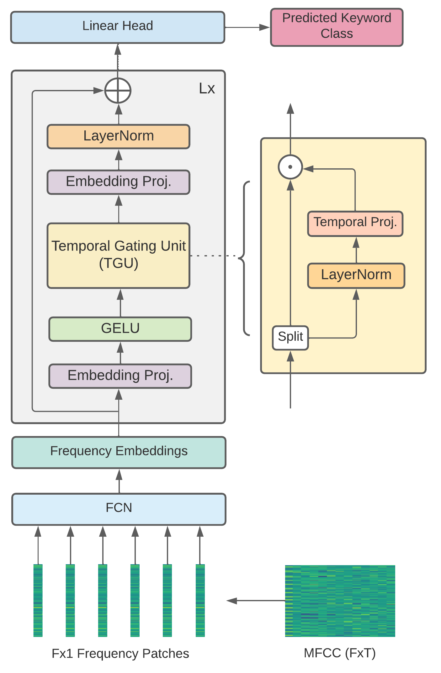
Figure 1: The Keyword-MLP architecture, consisting of L blocks (equation 2). Note that we move the LayerNorm to the end, before the skip-connection, different from Liu et al. (2021) where norm is applied at the beginning. ($\oplus$ represents a residual skip-connection, while $\odot$ represents element-wise product.)

The obtained ${\bm{X}}_{E}$ is passed through $L$ consecutive, identical gated-MLP (gMLP) blocks (Liu et al., 2021). On a high level, we can summarize the gMLP blocks used in KW-MLP as a pair of projections across the embedding dimension separated by a projection across the temporal dimension. The block can also be formulated with the following set of equations (omitting bias and normalization for the sake of conciseness):

$$\begin{split}{\bm{Z}}&=\sigma({\bm{X}}_{in}{\bm{U}})\\ \tilde{\bm{Z}}=g({\bm{Z}})&=g([{\bm{Z}}_{r}{\bm{Z}}_{g}])={\bm{Z}}_{r}\odot({\bm{Z}}_{g}^{T}{\bm{G}})^{T}\\ {\bm{X}}_{out}&=\tilde{\bm{Z}}{\bm{V}}\oplus{\bm{X}}_{in}\end{split}$$ (2)

First, we use the matrix ${\bm{U}}\in\mathbb{R}^{d\times{D}}$ to linearly project ${\bm{X}}_{in}$ from the embedding dimension $d$ to the projection dimension $D$ (essentially a matmul operation). $\sigma$ represents the GELU activation function. $g(Z)$ represents the the Temporal Gating Unit (TGU) shown in Figure 1. The input to TGU, ${\bm{Z}}$, is first split into ${\bm{Z}}_{r}$ and ${\bm{Z}}_{g}\in\mathbb{R}^{T\times{D/2}}$, the residual and the gate respectively. We use the matrix ${\bm{G}}\in\mathbb{R}^{T\times{T}}$ to performs the linear projection across the temporal axis. This is followed by the linear gating—an element-wise multiplication with the residual ${\bm{Z}}_{r}$. While the temporal projection operation can be implemented as passing ${\bm{Z}}_{g}$ transposed through a Dense(T, T) layer, in practice, it can be implemented more efficiently by instead passing ${\bm{Z}}_{g}$ through a Conv1D(T, T, 1) layer. $\tilde{\bm{Z}}\in\mathbb{R}^{T\times{D/2}}$ is projected back to the embedding dimension $d$ with the matrix ${\bm{V}}$ and then added with the skip-connected input ${\bm{X}}_{in}$.

The original gMLP paper (Liu et al., 2021) applies LayerNorm before the initial channel projection (analogous to embedding projections for images). We however find that applying norm after the second embedding projection results in a notably faster and more optimal convergence. Berg et al. (2021) also observe a similar phenomenon in their work.

The overall system is shown in Figure 1. In KW-MLP, we primarily use $L=12$ (12 consecutive gMLP blocks), embedding dim $d=64$, and projection dim $D=256$. We also explore a group of smaller KW-MLP models with shallower depth, i.e. $L=10,8,6$. The input MFCCs to the model are of shape $40\times 98$, where 40 is the number of frequency bins, and 98 is the number of timesteps. All settings are also shown in Table 2.

It is to be noted that the largest KW-MLP model has only 0.424M parameters, which is smaller than the smallest KWT variant (KWT-1 with 0.607M params) and much smaller than AST models (87M params). However, from Table 1 we can see that KW-MLP shows competitive accuracy with these models, particularly on the Speech Commands V2-35 benchmark.

3.1 Knowledge Distillation

In order to boost the accuracies of shallower KW-MLP variants, we use knowledge distillation (KD) (Hinton et al., 2015), using the KW-MLP model with $L=12$ as the teacher model. We use an annealed KD approach (Jafari et al., 2021) where the temperature parameter decreases every step following a cosine-annealing rule till it reaches 1. Other KD parameters, such as alpha, are shown in Table 2. We also do not use label smoothing when training with KD, as soft targets are obtained from teacher predictions.

Table 1: Comparison of Model Parameters and Accuracy on Google Speech Commands V2-12 and V2-35 benchmarks (Warden, 2018)

Method	Extra Knowledge	V2-12	V2-35	# Params (M)
Att-RNN  [2]		96.9	93.9	0.202
Res-15  [21]		98.0	96.4	0.237
MHAtt-RNN  [14]		98.0	97.27	0.743
AST-S  [6]	Pre. ImageNet		98.11	87
AST-P  [6]	Pre. ImageNet & Audioset		97.88	87
KWT-3  [1]	KD with MHAtt-RNN	98.56	97.69	5.361
KWT-2  [1]	KD with MHAtt-RNN	98.43	97.74	2.394
KWT-1  [1]	KD with MHAtt-RNN	98.08	96.95	0.607
KWT-3  [1]		98.54	97.51	5.361
KWT-2  [1]		98.21	97.53	2.394
KWT-1  [1]		97.72	96.85	0.607
KW-MLP		97.63	97.56	0.424
KW-MLP10		97.38	97.35	0.353
KW-MLP8		97.28	97.26	0.283
KW-MLP6		97.03	97.07	0.213
KW-MLP10	KD with KW-MLP	97.30	97.49	0.353
KW-MLP8	KD with KW-MLP	97.24	97.45	0.283
KW-MLP6	KD with KW-MLP	97.12	97.17	0.213

4 Experimental Details

We follow similar hyperparameters to Rybakov et al. (2020); Berg et al. (2021), with minor changes; all our hyperparameters and settings are shown in Table 2. For training, we use a smaller batch-size of 256, and train for 140 epochs. No other augmentation apart from Spectral Augmentation (Park et al., 2019) is applied (to enable fast training). As an additional regularization method, each gMLP block has a survival probability of 0.9 (alternatively, a 0.1 probability to drop each block). We run experiments on Google Speech Commands V2-12 and V2-35 benchmarks, following the standard protocol described in Warden (2018).

As seen from Table 1, the largest KW-MLP model has only 424K parameters, which is much fewer than the KWT models, while having comparable accuracy. Furthermore, since we do not apply expensive run-time augmentations like resampling, time-shifting, adding background noise, mixup, etc. (used by (Rybakov et al., 2020; Berg et al., 2021; Gong et al., 2021)), it is possible to train KW-MLP models in a very short time on free cloud compute such as the NVIDIA Tesla K80 or Tesla P100 provided by Google Colab and Kaggle.

As a trade-off for fast training, a limitation of the KW-MLP experiments is that the effect of various augmentation methods have not been explored. This is more apparent in the V2-12 task, which contains much fewer training examples ($\sim 37000$) than the V2-35 task ($\sim 84000$). The KW-MLP model does not generalize as well here, as compared to V2-35.

Table 2: Overview of Hyper-Parameters and Settings

Training			Augmentation			Model
Epochs	140		# Time Masks	2		# Blocks, $L$	12
Batch Size	256		Time Mask Width	[0, 25]		Input Shape	$40\times 98$
Optimizer	AdamW		# Freq Masks	2		Patch Size	$40\times 1$
Learning Rate	0.001		Freq Mask Width	[0, 7]		Dim, $d$	64
Warmup Epochs	10					Dim Proj.	256
Scheduling	Cosine					# Classes	35
Regularization			Audio Processing			KD
Label Smoothing	0.1		Sampling Rate	16000		$\alpha$	0.9
Weight Decay	0.1		Window Length	30 ms		Init Temp	5.0
Block Survival Prob.	0.9		Hop Length	10 ms
			n_mfcc	40

5 Temporal Projection Matrices

We additionally visualize the weights of the temporal gating unit (the temporal projection matrix ${\bm{G}}\in\mathbb{R}^{T\times{T}}$ in equation 2). Interestingly, we can observe that our model learns weights which seem similar to diagonal, identity, or toeplitz matrices. This suggests that KW-MLP may partially learn a form of shift-invariance, which is necessary for the keyword spotting task. For instance, in a 1 second audio clip, a keyword can occur at different temporal positions; so the model needs to be invariant to temporal shift.

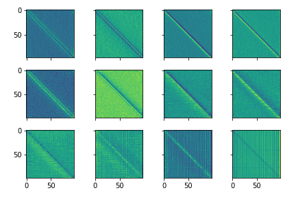
Figure 2: Visualization of the temporal projection matrices, ${\bm{G}}$, for each of the $L=12$ gMLP blocks of KW-MLP. The matrices are arranged in row major order.

6 Conclusion

The Keyword-MLP has shown itself to be an efficient solution to the keyword spotting task, and an alternative to self-attention-based methods. We hope that we provide an additional avenue of future research in audio and speech domains, particularly when resource-efficiency is concerned.

References

- Berg et al. (2021) Axel Berg, Mark O’Connor, and Miguel Tairum Cruz. Keyword Transformer: A Self-Attention Model for Keyword Spotting. In Proc. Interspeech 2021, pp. 4249–4253, 2021. doi: 10.21437/Interspeech.2021-1286.
- de Andrade et al. (2018) Douglas Coimbra de Andrade, Sabato Leo, Martin Loesener Da Silva Viana, and Christoph Bernkopf. A neural attention model for speech command recognition. arXiv preprint arXiv:1808.08929, 2018.
- Deng et al. (2009) Jia Deng, Wei Dong, Richard Socher, Li-Jia Li, Kai Li, and Li Fei-Fei. Imagenet: A large-scale hierarchical image database. In 2009 IEEE Conference on Computer Vision and Pattern Recognition, pp. 248–255, 2009. doi: 10.1109/CVPR.2009.5206848.
- Dosovitskiy et al. (2020) Alexey Dosovitskiy, Lucas Beyer, Alexander Kolesnikov, Dirk Weissenborn, Xiaohua Zhai, Thomas Unterthiner, Mostafa Dehghani, Matthias Minderer, Georg Heigold, Sylvain Gelly, et al. An image is worth 16x16 words: Transformers for image recognition at scale. arXiv preprint arXiv:2010.11929, 2020.
- Gemmeke et al. (2017) Jort F. Gemmeke, Daniel P. W. Ellis, Dylan Freedman, Aren Jansen, Wade Lawrence, R. Channing Moore, Manoj Plakal, and Marvin Ritter. Audio set: An ontology and human-labeled dataset for audio events. In Proc. IEEE ICASSP 2017, New Orleans, LA, 2017.
- Gong et al. (2021) Yuan Gong, Yu-An Chung, and James Glass. AST: Audio Spectrogram Transformer. In Proc. Interspeech 2021, pp. 571–575, 2021. doi: 10.21437/Interspeech.2021-698.
- Hinton et al. (2015) Geoffrey Hinton, Oriol Vinyals, and Jeff Dean. Distilling the knowledge in a neural network. arXiv preprint arXiv:1503.02531, 2015.
- Jafari et al. (2021) Aref Jafari, Mehdi Rezagholizadeh, Pranav Sharma, and Ali Ghodsi. Annealing knowledge distillation. arXiv preprint arXiv:2104.07163, 2021.
- Liu et al. (2021) Hanxiao Liu, Zihang Dai, David R So, and Quoc V Le. Pay attention to mlps. arXiv preprint arXiv:2105.08050, 2021.
- Majumdar & Ginsburg (2020) Somshubra Majumdar and Boris Ginsburg. Matchboxnet: 1d time-channel separable convolutional neural network architecture for speech commands recognition. arXiv preprint arXiv:2004.08531, 2020.
- Melas-Kyriazi (2021) Luke Melas-Kyriazi. Do you even need attention? a stack of feed-forward layers does surprisingly well on imagenet. arXiv preprint arXiv:2105.02723, 2021.
- Mordido et al. (2021) Gonçalo Mordido, Matthijs Van Keirsbilck, and Alexander Keller. Compressing 1d time-channel separable convolutions using sparse random ternary matrices. arXiv preprint arXiv:2103.17142, 2021.
- Park et al. (2019) Daniel S Park, William Chan, Yu Zhang, Chung-Cheng Chiu, Barret Zoph, Ekin D Cubuk, and Quoc V Le. Specaugment: A simple data augmentation method for automatic speech recognition. arXiv preprint arXiv:1904.08779, 2019.
- Rybakov et al. (2020) Oleg Rybakov, Natasha Kononenko, Niranjan Subrahmanya, Mirko Visontai, and Stella Laurenzo. Streaming keyword spotting on mobile devices. arXiv preprint arXiv:2005.06720, 2020.
- Tang & Lin (2018) Raphael Tang and Jimmy Lin. Deep residual learning for small-footprint keyword spotting. In 2018 IEEE International Conference on Acoustics, Speech and Signal Processing (ICASSP), pp. 5484–5488. IEEE, 2018.
- Teacher et al. (1967) C Teacher, H Kellett, and L Focht. Experimental, limited vocabulary, speech recognizer. IEEE Transactions on Audio and Electroacoustics, 15(3):127–130, 1967.
- Tolstikhin et al. (2021) Ilya Tolstikhin, Neil Houlsby, Alexander Kolesnikov, Lucas Beyer, Xiaohua Zhai, Thomas Unterthiner, Jessica Yung, Daniel Keysers, Jakob Uszkoreit, Mario Lucic, et al. Mlp-mixer: An all-mlp architecture for vision. arXiv preprint arXiv:2105.01601, 2021.
- Touvron et al. (2021a) Hugo Touvron, Piotr Bojanowski, Mathilde Caron, Matthieu Cord, Alaaeldin El-Nouby, Edouard Grave, Gautier Izacard, Armand Joulin, Gabriel Synnaeve, Jakob Verbeek, et al. Resmlp: Feedforward networks for image classification with data-efficient training. arXiv preprint arXiv:2105.03404, 2021a.
- Touvron et al. (2021b) Hugo Touvron, Matthieu Cord, Matthijs Douze, Francisco Massa, Alexandre Sablayrolles, and Hervé Jégou. Training data-efficient image transformers & distillation through attention. In International Conference on Machine Learning, pp. 10347–10357. PMLR, 2021b.
- Vaswani et al. (2017) Ashish Vaswani, Noam Shazeer, Niki Parmar, Jakob Uszkoreit, Llion Jones, Aidan N Gomez, Łukasz Kaiser, and Illia Polosukhin. Attention is all you need. In Advances in neural information processing systems, pp. 5998–6008, 2017.
- Vygon & Mikhaylovskiy (2021) Roman Vygon and Nikolay Mikhaylovskiy. Learning efficient representations for keyword spotting with triplet loss. arXiv preprint arXiv:2101.04792, 2021.
- Warden (2018) Pete Warden. Speech commands: A dataset for limited-vocabulary speech recognition. arXiv preprint arXiv:1804.03209, 2018.
- Zhang & Koishida (2017) Chunlei Zhang and Kazuhito Koishida. End-to-end text-independent speaker verification with triplet loss on short utterances. In Interspeech, pp. 1487–1491, 2017.