Modeling the Spectral Diversity of Quasars in the Sixteenth Data Release from the Sloan Digital Sky Survey

Abstract

We present a new approach to capturing the broad diversity of emission line and continuum properties in quasar spectra. We identify populations of spectrally similar quasars through pixel-level clustering on 12,968 high signal-to-noise ratio (S/N) spectra from the Sloan Digital Sky Survey (SDSS) in the redshift range of $1.57<z<2.4$. Our clustering analysis finds 396 quasar spectra that are not assigned to any population, 15 misclassified spectra, and 6 quasars with incorrect redshifts. We compress the quasar populations into a library of 684 high S/N composite spectra, anchored in redshift space by the Mg ii emission line. Principal component analysis on the library results in an eigenspectrum basis spanning $1067-4007$ Å. We model independent samples of SDSS quasar spectra with the eigenbasis, allowing for a free redshift parameter. Our models achieve a median reduced $\chi^{2}$ on non-broad absorption line quasar spectra that is reduced by 8.5% relative to models using the eigenspectra from the SDSS spectroscopic pipeline. A significant contribution to the relative improvement is from the ability to reconstruct the range of emission line variation. The redshift estimates from our model are consistent with the Mg ii emission line redshift with an average offset that displays 51.4% less redshift-dependent variation relative to the SDSS eigenspectra. Our method for developing quasar spectra models can improve automated classification and predict the intrinsic spectrum in regions affected by intervening absorbers such as Ly$\alpha$, C iv, and Mg ii, thus benefiting studies of large-scale structure.

1. Introduction

Quasars exhibit distinct spectral features in the UV and optical wavelengths, featuring broad and narrow emission lines with a continuum that can be approximated by a power law. The similarity permits co-addition of spectra to characterize general properties and amplify weaker spectral features (e.g. Francis et al., 1991; Vanden Berk et al., 2001; Tammour et al., 2015; Harris et al., 2016; Jensen et al., 2016). While the first-order similarity is impressive, emission line profiles and continuum slopes vary across the full population and in time. Reverberation mapping provides insight into the structure of the emitting regions and the central black hole (see Shen et al., 2015; Kaspi et al., 2021; Yu et al., 2021, for example); however, a comprehensive model that explains the full range of diversity is lacking (e.g. Ruan et al., 2014; Luo et al., 2015; Dyer et al., 2019; Matthews et al., 2020).

Complications in spectral modeling stem from variation at all wavelengths. Within the same quasar spectrum, the locations of different emissions lines are offset nonuniformly from the systemic redshift (e.g. Hewett & Wild, 2010; Shen et al., 2016). Across different spectra, emission lines exhibit varying degrees of asymmetries in their profiles. Some quasars also display broad, blue-shifted absorption troughs associated with prominent emission lines, referred to as broad absorption line (BAL) quasars (e.g. Weymann et al., 1991; Hall et al., 2002). The number of BALs in a spectrum, along with their corresponding velocity widths and blueshifts, varies from one BAL quasar to the next.

Without an accepted theoretical model, modeling efforts rely on empirical trends in spectral properties and correlations between features. For example, the equivalent width of broad emission lines is known to be anticorrelated with continuum luminosity, referred to as the Baldwin Effect. The anticorrelation was first observed with the C iv emission line (Baldwin, 1977) and later confirmed in other lines (see Shields, 2007, for a review). The physical mechanism that drives the Baldwin Effect is still debated. Principal Component Analysis (PCA) is a mathematical tool that reveals significant sources of signal variance and empirical correlations between features. Boroson & Green (1992) performed PCA on measured properties of low redshift quasars, revealing a strong relationship between the strengths of Fe ii and [O iii] emission and properties of the H$\beta$ emission line, known as Eigenvector 1 (EV1). EV1 trends are believed to be related to the Eddington Ratio (e.g. Boroson, 2002; Shen & Ho, 2014).

PCA implemented directly on quasar spectra captures intrinsic variance on the level of individual flux densities. Eigenspectra covering the UV wavelengths are connected to the Baldwin Effect (e.g. Shang et al., 2003; Yip et al., 2004) and reveal that significant variance can be attributed to the cores of broad emission lines and continuum slopes (e.g. Francis et al., 1992; Rochais et al., 2017). In the first application of PCA on quasar spectra, Francis et al. (1992) demonstrated that linear combinations of a small number of eigenspectra can adequately reconstruct observed data from the Large, Bright Quasar Survey (Hewett et al., 1995). PCA has since become a popular method for developing data-driven models of quasar spectra (e.g. Suzuki et al., 2005; Suzuki, 2006; Pâris et al., 2011, 2012; Davies et al., 2018; Guo & Martini, 2019). A single set of four eigenspectra was used for automatic identification and redshift estimation for all quasar spectra in the Baryon Oscillation Spectroscopic Survey (BOSS; Dawson et al., 2013) and the extended Baryon Oscillation Spectroscopic Survey (eBOSS; Dawson et al., 2016), as described in Bolton et al. (2012, hereafter B12). Yip et al. (2004), however, argue that because spectral diversity is dependent on both redshift and luminosity (e.g. Vanden Berk et al., 2004; Jensen et al., 2016), there does not exist a compact set of quasar eigenspectra that adequately describes all quasars. The authors suggest that eigenspectra developed for specific ranges in this parameter space are necessary for accurate modeling.

In this work, we implement a technique that clusters quasar spectra in the redshift range $1.57<z<2.4$ based on similarity at the pixel level. We use quasar spectra from the Sixteenth Data Release (DR16; Ahumada et al., 2020) of the fourth generation of the Sloan Digital Sky Survey (SDSS-IV; Blanton et al., 2017). Potential contaminants and peculiar quasars in the sample are easily discovered, as highly dissimilar spectra naturally segregate. We use the clusters of similar quasar spectra to construct a library of high signal-to-noise ratio (S/N) composite spectra that is representative of the spectral diversity across the entire sample. We perform PCA on the library and compare the modeling performance of the resulting eigenspectra to that of the B12 eigenspectra. Our method for developing quasar eigenspectra differs from previous work, as PCA is performed not on a selection of individual quasar spectra but rather on composite spectra built from quasar populations with low internal diversity, promoting representation of recurrent spectral features. In addition, the high S/N of the composite spectra allows us to apply a redshift correction to the PCA training sample through measurement of the Mg ii emission line location and therefore mitigate potential offsets.

In Section 2, we describe the training sample of quasar spectra selected for our clustering analysis. We also detail the quasar samples used for testing the modeling performance of the eigenspectra. In Section 3, we introduce our clustering technique, present the clustering results, and outline how we transform clusters of similar spectra into a library of high S/N composite spectra. In Section 4, we perform PCA on the library and present our eigenspectra. We select the number of eigenspectra for modeling spectra of the test samples and compare the modeling performance to B12 eigenspectra. In Section 5, we summarize our results from this work and outline future improvements with data from the Dark Energy Spectroscopic Instrument (DESI; DESI Collaboration et al., 2016a, b).

2. Data

This work uses quasar spectra and their classifications from DR16 of SDSS-IV collected as a part of the BOSS and eBOSS programs. A primary goal of BOSS and eBOSS was to constrain cosmological parameters through measurements of the baryon acoustic oscillation feature in the distribution of matter. The final cosmological implications from BOSS and eBOSS are summarized in Alam et al. (2021).

Quasars were a primary spectroscopic target of BOSS and eBOSS. At $z<2.2$, quasars are used as direct tracers of the matter distribution (Neveux et al., 2020; Hou et al., 2021), while at higher redshifts the Ly$\alpha$ forest observed as absorption in quasar spectra traces the matter distribution (du Mas des Bourboux et al., 2020). We select quasar samples for this study from the final quasar catalog of DR16 (DR16Q; Lyke et al., 2020). This section summarizes the spectroscopic data and selection criteria for the training sample used in our clustering analysis. We then describe the calibration and filtering procedures applied to the training sample to maximize the information gained from clustering. Finally, the test samples for evaluating the performance of our eigenspectra models are presented.

2.1. Spectroscopic Data

The BOSS and eBOSS programs used a pair of identical multi-object fiber spectrographs (Smee et al., 2013) on the 2.5 m Sloan telescope (Gunn et al., 2006) at Apache Point Observatory. Observations were taken using aluminum plates, each of which subtended $3\arcdeg$ on the sky. Each plate featured 1000 holes drilled $2\arcsec$ in diameter at locations corresponding to calibration, stellar, galaxy, or quasar targets. Once an observation with a plate was completed, the 1000 spectra were processed and classified (Bolton et al., 2012). The method for selecting quasar targets in BOSS and eBOSS is detailed in Ross et al. (2012) and Myers et al. (2015), respectively.

2.2. Training Sample

We apply a clustering technique to a training sample of quasar spectra to identify groups that possess similar spectral features. The training sample must capture the diversity of continuum and emission line properties to adequately represent the entire quasar population. Additionally, the training sample must be relatively free of nonintrinsic spectral features to increase the true physical similarity within clusters. These two factors are the primary considerations when selecting the training sample.

The training sample is selected based on redshift, balnicity, and S/N of the spectra. We use the Z_PCA redshifts in DR16Q, which were estimated using the four B12 eigenspectra (see Section 4 of Bolton et al., 2012) plus a three-term polynomial in $\log\lambda$ for broadband. Only quasars with reliable redshift estimates are included in the training sample by requiring ZWARN_PCA = 0. Quasar spectra containing BALs are excluded by requiring a BAL_PROB attribute of zero. This exclusion ensures that clusters form based on intrinsic similarity. Finally, the average S/N ratio per pixel is determined over the entire observed spectrum after excluding pixels identified as having poor sky subtraction. A minimum average S/N ratio of 10 per pixel is required for the training sample.

The redshift range is selected to maximize the number of spectral features covered by the training sample. The identification of BALs requires the presence of the C iv emission line at the rest-frame wavelength of 1549 Å, leading to a minimum redshift of $z=1.57$. The upper limit in redshift is set to $z=2.4$ by requiring that the Mg ii emission line be present at a reasonably high S/N. The resulting training sample contains 12,968 quasars. As shown in Table 1, the training sample is binned into four discrete subsets of width $\Delta z\approx 0.2$. Clustering is performed within each redshift bin independently to account for potential redshift evolution.

All spectra within a redshift bin are cropped to a common rest-frame wavelength range defined from $\lambda_{min}$ to $\lambda_{max}$. $\lambda_{min}$ is set by the bluest pixel of the lowest redshift spectrum in the bin, and $\lambda_{max}$ is set by the reddest pixel in the highest redshift spectrum in the bin. The flux of each spectrum is normalized according to its median computed over the common wavelength range. The rest-frame values of $\lambda_{min}$ and $\lambda_{max}$ for the redshift bins are reported in Table 1.

Table 1The number of quasars in each redshift bin and wavelength range used for clustering

Redshift Range	Quasars	$\lambda_{min}$ (Å)	$\lambda_{max}$ (Å)
$1.57<z<1.8$	3201	1396.69	3714.50
$1.8<z<2.0$	3393	1273.21	3460.19
$2.0<z<2.2$	3006	1189.60	3233.70
$2.2<z<2.4$	3368	1115.32	3057.03

As a simple diagnostic of diversity, we explore the distribution of equivalent width of the C iv emission line within each redshift bin. The equivalent width is determined through fitting a double Gaussian to the continuum-subtracted flux in the range $1510-1590$ Å. The continuum flux in the region of the C iv emission line is estimated by fitting a power law over the ranges $1430-1450$ Å and $1680-1700$ Å. The location, width, and amplitude parameters for each Gaussian vary independently as expected from kinematics of gas responsible for narrow and broad emission. The equivalent width is calculated only for C iv emission regions containing 20 or more reliable pixels. The mean and standard deviation of the equivalent width for the bins are $24.87\pm 11.76$, $24.23\pm 10.84$, $23.41\pm 10.62$, and $22.61\pm 10.21$, in order of increasing redshift. Due to selection effects, higher luminosity objects are more likely to be observed with increasing redshift; thus, the apparent decrease in equivalent width is the Baldwin Effect for C iv.

The distribution of absolute magnitude in the i-band as a function of redshift for quasars in DR16Q is shown in Figure 1. The training sample is highlighted in red. The training selection is intrinsically more luminous than the general population owing to the S/N requirement. In addition, the training sample trends toward higher luminosity with increasing redshift. This trend explains the decreasing equivalent width of the C iv emission line with increasing redshift that was described in the previous paragraph.

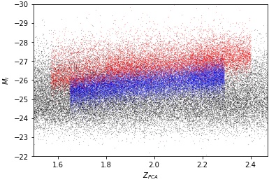
Figure 1.— The black data points correspond to the absolute i-band magnitude of a 10% random sampling of all quasars in DR16Q as a function of redshift. Only quasars detected at $1\sigma$ in the i-band are displayed. The quasars selected for the training sample are shown in red. The quasars selected for the standard test sample are shown in blue. The vertical lines indicate the redshift bins of the training sample.

The quasar spectra in the training sample are calibrated to minimize spurious signal. All spectra are corrected for galactic extinction using the Fitzpatrick model (Fitzpatrick, 1999) and dust extinction map from Schlegel, Finkbeiner, & Davis (1998). Pixels flagged by the eBOSS pipeline as contaminated by sky emission are masked. Flux measurements at $\lambda_{obs}<3610.5$ Å are removed owing to uncertainty in flux and wavelength calibration. Each spectrum is then shifted to its rest-frame wavelength solution based on the Z_PCA redshift estimate. Pixels in the Ly$\alpha$ forest at $\lambda_{em}<1216$ Å are masked to eliminate stochasticity arising from external sources.

We next identify and remove narrow absorption lines (NALs) in the quasar spectra. NALs are imprinted by diffuse circumgalactic medium (CGM) along the line of sight (see Tumlinson et al., 2017). The intrinsic spectrum of each quasar is estimated by applying an error-weighted Gaussian smoothing filter with a dispersion of 8 pixels. NALs are identified at pixels where the ratio of measured flux to smoothed flux deviates negatively by more than three standard deviations. Pixels with suspected absorption lines are masked. An application of the NAL filter is shown in Figure 2.

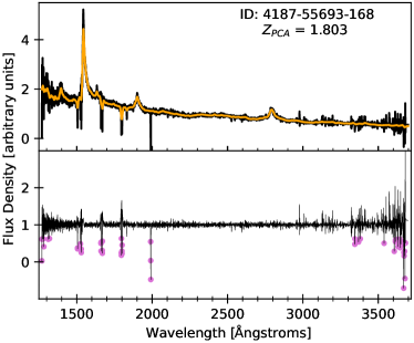
Figure 2.— An example of the NAL filter applied to a quasar spectrum. Top: the measured flux density is shown in black, with the estimated spectrum from the Gaussian smoothing filter overlaid in orange. The ID code corresponds to the unique PLATE-MJD-FIBERID of every SDSS spectrum. Bottom: the ratio of measured flux to smoothed flux is shown in black. Pixels at which the ratio deviates negatively by greater than three standard deviations are marked in purple. These flux decrements likely originate from CGM absorption and are masked in our clustering analysis.

2.3. Standard Test Sample

A clustering analysis applied to the training sample is used to derive quasar eigenspectra (discussed in Section 4.1). We evaluate the ability of these eigenspectra to model an independent test sample of quasar spectra. The standard test sample is selected based on redshift and S/N requirements, excluding quasars with a nonzero BAL_PROB attribute. The redshift range of the standard test sample is cropped to $1.65<z<2.29$ to allow for a free redshift parameter in the fitting. Only spectra with a ZWARN_PCA attribute of zero are included. Flux measurements at rest-frame wavelengths shorter than 1216 Å according to Z_PCA are given a weight of zero to mask the Ly$\alpha$ forest. The quasar spectra in the standard test sample have an average S/N ratio per pixel over the entire spectrum ranging between 5 and 10. The upper bound in S/N is imposed to avoid overlap with the training sample.

The standard test sample contains 26,498 quasars. The distribution of absolute magnitude in the i-band for the standard test sample as a function of redshift is highlighted in blue in Figure 1. As with the training sample, the S/N requirement leads to intrinsically brighter quasar sources than the general population and shows a trend of increasing luminosity with redshift.

2.4. BAL Test Sample

BALs are observed in a significant fraction of quasar spectra. In the UV and visible wavelengths, the fraction is reported between 10% and 30% (e.g. Trump et al., 2006; Pâris et al., 2012; Guo & Martini, 2019). Recent work (e.g. Rankine et al., 2020) supports the theory that quasars containing BALs are not a distinct class of quasars. Rather, the BALs most likely arise as a result of orientation effects that place outflowing gas along the line of sight, with all quasars having some probability to observed with BALs. We test the ability of our eigenspectra to model the unabsorbed spectra of a sample of BAL quasars.

The BAL test sample is selected from the Guo & Martini (2019) BAL Quasar Catalog. The quasars in the catalog are from DR14 of SDSS-IV (Abolfathi et al., 2018) and were classified as BAL quasars using a convolutional neural network. The catalog contains the BAL_PROB determined by the neural network and the most robust redshift estimate for each quasar, Z. Only objects with a BAL_PROB of greater than 0.5 are included in the BAL Quasar Catalog. Quasars within the redshift range $1.65<z<2.29$ are selected for our BAL test sample. The BAL features recorded in the catalog are measured relative to Z so the sample is selected using this redshift estimate rather than Z_PCA. We set a minimum average S/N ratio per pixel requirement of 5. We do not impose a maximum value on the S/N ratio per pixel, as all quasars in the training sample have a BAL_PROB of zero, and thus there is no overlap between the two samples. The final BAL test sample contains 12,431 quasars.

The BAL Quasar Catalog includes both the blueshifts and velocity widths of absorption troughs associated with the C iv and Si iv emission lines. This information is used to mask the regions of a spectrum contaminated by BALs with velocity widths greater than 450 km s^-1. In addition to masking the BAL troughs, the Ly$\alpha$ forest at $\lambda_{em}<1216$ Å is masked. We then model the remaining unmasked pixels with our eigenspectra.

3. Clustering

We use a clustering technique as a form a data compression. We transform 12,968 individual spectra into a library of composite spectra built from clusters of quasars with similar spectra. In this section, we discuss our clustering method and the results within each redshift bin. We then describe the objects that fail to cluster and examine possible causes. Lastly, we outline the procedure for transforming the clusters into a library of high S/N composite quasar spectra corrected to the rest-frame wavelength of the Mg ii emission line.

3.1. SetCoverPy

SetCoverPy (Zhu, 2016) is a classification algorithm based on the Set Cover Problem (SCP). A full description of SetCoverPy and the SCP is beyond the scope of this paper, and we refer the reader to Zhu (2016) for more details. In brief, SetCoverPy identifies representatives of a sample based on a similarity (or distance) metric between instances. Instances with strong similarity (or a small distance) are able to represent each other. The threshold for two instances to be considered similar enough such that they can represent each other is a free parameter determined by the user. The goal of SetCoverPy is to find an optimal set of instances that can represent the entirety of the sample at the minimum cost. These representative instances are dubbed archetypes. If all instances have uniform cost to be labeled an archetype, the solution is the minimum number of archetypes necessary to represent the sample. A single instance may be represented by multiple archetypes or be an archetype only for itself.

Implementing SetCoverPy requires selecting a distance metric to measure the similarity of instances and defining the cost for each instance to be labeled an archetype. Given a minimum distance within which pairs of instances can be considered similar and a pairwise distance matrix, SetCoverPy returns a list of archetypes of the input sample. We use SetCoverPy with a few modifications on our training sample of quasars to identify clusters with similar spectra.

3.2. SetCoverPy on Quasar Spectra

We find clusters of similar quasar spectra in each redshift bin of the training sample using spectral archetypes identified with SetCoverPy. We measure the similarity of quasar spectra using the reduced $\chi^{2}$ statistic (see Section 3.2.1). All quasar spectra are assigned equal cost; thus, SetCoverPy returns the minimum number of archetypes necessary to represent every spectrum in a redshift bin. We treat quasar archetypes as cluster centers around which we build clusters. The cluster members are assigned based on the minimum distance used to determine the archetypes.

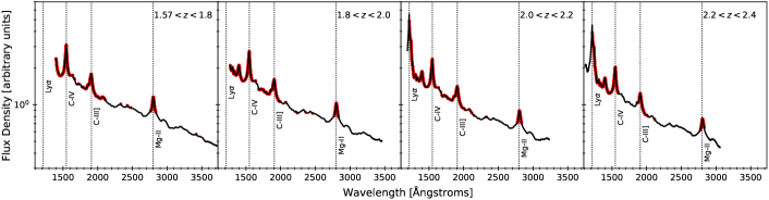
Figure 3.— The error-weighted mean spectrum of each redshift bin is shown in black. The pixels that exhibit spectral diversity in the 68th percentile or higher are shown in red. Pixels at wavelengths $<1216$ Å are excluded from the percentile cut due to the presence of the Ly$\alpha$ forest. The rest-frame wavelengths of Ly$\alpha$, C iv, C iii], and Mg ii emission are indicated by vertical lines.

A single quasar spectrum may fall within the minimum distance to multiple archetypes. The quasar is assigned to multiple clusters in this case. We find this overlap feature especially desirable because there are no clear boundaries from one subclass of quasars to the next. Rather, there exist natural gradients and/or overlap between populations. Deciding where to draw the boundary line along these gradients is frequently arbitrary and may lead to the misclassification of near-boundary objects (for an example of this problem with galaxy populations, see Pandey, 2020).

Further, there are individual quasar spectra that are archetypes only for themselves, not falling within the minimum distance to any other spectrum. We define quasars that are archetypes only for themselves as cluster outliers. We introduce an iterative procedure for reducing the number of cluster outliers and consequently increasing diversity coverage in the library of composite quasar spectra. This procedure is detailed in Section 3.2.2.

3.2.1 Distance Metric

We adopt the reduced $\chi^{2}$ statistic as the distance metric for measuring spectral similarity in the training sample. The $\chi^{2}$ statistic is analogous to a weighted squared Euclidean distance in N-dimensional space. The reduced $\chi^{2}$ between two quasar spectra in a redshift bin is computed as

$$\chi_{ij}^{2}=\frac{1}{N-2}\sum_{n=1}^{N}\frac{(f_{i}(\lambda_{n})-c\lambda^{\Delta\alpha_{\lambda}}f_{j}(\lambda_{n}))^{2}}{\sigma_{i}(\lambda_{n})^{2}+(c\lambda^{\Delta\alpha_{\lambda}}\sigma_{j}(\lambda_{n}))^{2}}$$ (1)

where N is the number of pixels covered by the common wavelength range that have reliable measurements for both spectra ($\frac{1}{\sigma_{i}^{2}\sigma_{j}^{2}}>0$). In pixel-level clustering, the difference in power-law spectral indices between two spectra in a pair will be present across all pixels and can dominate the $\chi^{2}$. The $c\lambda^{\Delta\alpha_{\lambda}}$ term accounts for this difference, effectively removing the power-law component of the continuum from consideration in the distance metric. The two parameters, c and $\Delta\alpha_{\lambda}$, are determined by minimizing the reduced $\chi^{2}$ in every pairwise comparison of quasar spectra. Symmetry is maintained in the distance matrix by always applying this term to the higher S/N spectrum of the pair.

We found that computing the reduced $\chi^{2}$ using every pixel in the common wavelength range allows continuum-dominated portions of the spectra to dilute the distance statistic. We therefore focus the reduced $\chi^{2}$ statistic on the pixels that exhibit the most flux diversity in each redshift bin to increase the information content. These pixels were identified by computing the average reduced $\chi^{2}$ about the error-weighted mean using all spectra in the bin. Those pixels in the 68th percentile and above are highlighted in the mean spectrum of each bin in Figure 3. Only the highlighted pixels factor into the reduced $\chi^{2}$ statistic between quasar spectra pairs. This selection of pixels focuses the comparison primarily on the prominent emission features. The pixels blueward of $1216$ Å do not factor into determining the 68th percentile cut on diversity, as these are masked owing to the presence of Ly$\alpha$ forest.

3.2.2 Iterative Clustering

Table 2Final Clustering Statistics

Redshift	Initial	Number of	Largest	Average	Initial Number	Final Number
Bin	Reduced $\chi^{2}$	Clusters	Cluster Size	Cluster Size	of Outliers	of Outliers
$1.57<z<1.8$	1.071	194	822	110	547	34
$1.8<z<2.0$	1.147	183	1169	164	625	71
$2.0<z<2.2$	1.350	152	1001	166	639	92
$2.2<z<2.4$	1.573	160	1191	182	914	206

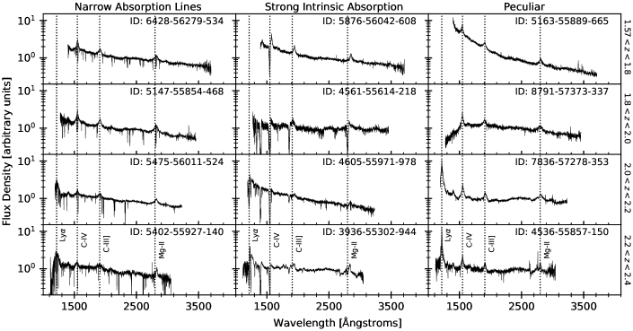
Figure 4.— Example spectra from each redshift bin that belong to one of the three primary outlier classes: spectra with unmasked NALs imprinted by CGM, spectra with strong intrinsic absorption, and spectra with peculiar shapes or features such as the flux calibration error seen in the peculiar spectrum of the highest redshift bin. The spectra have been shifted to the rest-frame wavelength solution according to the Z_PCA redshift estimate. Quasar spectra with strong intrinsic absorption often also have an incorrect redshift estimate.

The minimum distance within which quasar pairs can be considered similar is the only free parameter in SetCoverPy; therefore, its selection dictates the solution. A larger minimum distance will reduce the number of archetypes necessary to represent the entire sample of quasars. Conversely, a smaller minimum distance results in a larger number of clusters with less internal diversity. In addition, as the minimum reduced $\chi^{2}$ is decreased, more quasars will be identified as cluster outliers.

We select the minimum reduced $\chi^{2}$ for each redshift bin by balancing the number of cluster outliers and the size of the largest cluster. To avoid overfitting the minimum distance parameter, each redshift bin is randomly subsampled three times. SetCoverPy is implemented on each random sample over a range of minimum reduced $\chi^{2}$ values. The fraction of quasars labeled as outliers and the fraction of quasars assigned to the largest cluster are recorded in each iteration. We choose the minimum reduced $\chi^{2}$ value for each redshift bin where the averages of these two fractions over the three subsamples are approximately equal. The equality occurs at the reduced $\chi^{2}$ values given in Table 2. The minimum reduced $\chi^{2}$ increases with redshift.

The resulting outlier fraction in each redshift bin lies between 15% and 30%. Neglecting all of the outliers reduces the diversity coverage of clusters. Inspection of the cluster outliers reveals that many fall on the boundary of the minimum distance cutoff from one or more of the archetypes. We preserve the initial cluster structure and retrieve outliers by adding them to existing clusters in an iterative process. The process also permits outliers to form new clusters.

The outlier fraction is reduced by incrementally increasing the minimum reduced $\chi^{2}$ by 10% of the original value for the redshift bin. SetCoverPy is run on a data set containing only the archetypes and cluster outliers with the increased minimum distance value. The quasar archetypes are assigned a cost of zero since they have already been assigned as cluster centers. The outliers are assigned a uniform cost of one. Any outlier that can be represented by an existing archetype(s) in the new run of SetCoverPy is added to the cluster(s) centered on that archetype(s). If an outlier is determined to be an archetype of the updated data set, representing N other outliers, it is added to the list of archetypes. The outliers within the minimum distance to the new archetype then form a cluster. We repeat this procedure by increasing the minimum reduced $\chi^{2}$ another 10% from the original value and implementing SetCoverPy on the updated list of archetypes and remaining outliers. The minimum reduced $\chi^{2}$ value is increased until it reaches 150% the original value. The results of clustering in each bin are detailed in Table 2.

3.2.3 Outliers

We identify three broad categories of outliers through visual inspection of their spectra. Outlier spectra most commonly have several unmasked NALs, strong intrinsic absorption features from high column density associated absorbers, or truly peculiar spectral shapes or features. Outlier spectra also result from errors in flux calibration. In Figure 4, we show examples of outlier quasar spectra that fall into each of the three primary categories. The PCA redshift estimate is often incorrect for quasars in the first two of these categories. The incorrect redshift estimates are particularly evident in a few examples of the outlier quasar spectra with strong intrinsic absorption. We also find five outlier spectra from the highest redshift bin with incorrect redshifts where the C iv emission line was mistaken for Ly$\alpha$ in the PCA fit and one outlier in the lowest redshift bin where the C iii] emission line was mistaken for C iv. Lastly, we find one outlier spectrum that is a misclassified galaxy.

The outlier spectra that exhibit NALs from CGM indicate a shortcoming of the NAL filter (see Section 2.3). The filter fails to adequately estimate the intrinsic spectrum in these cases. Visual inspection reveals that the vast majority of the quasar spectra with unmasked CGM absorption are not intrinsically peculiar. Rather, the spurious absorption features drive the pairwise reduced $\chi^{2}$ to higher values. Further, the occurrence of outliers with spectra featuring heavy CGM absorption increases with redshift. From the low to high redshift bin, we identify 2, 8, 32, and 80 cluster outliers as having an excess of unmasked NALs. In future studies, a more aggressive approach to identifying and removing NALs may be necessary.

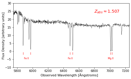
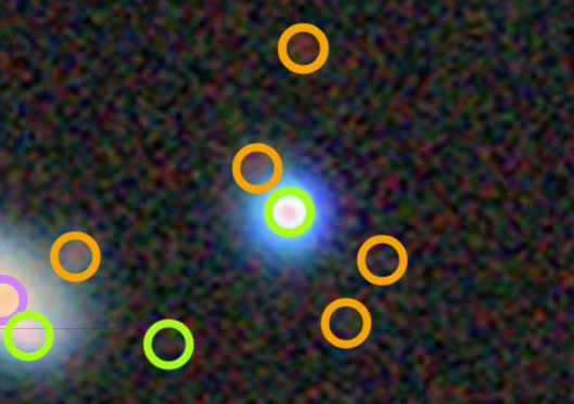
Figure 5.— Top: a region of the observer-frame spectrum of an outlier quasar at $z=2.028$ featuring a candidate absorption system at $z\approx 1.507$. Bottom: imaging data from DR9 of the DESI Legacy Imaging Survey centered on the quasar. Sources in DR9 are indicated with circles. There is a source to the northwest of the quasar that may be associated with the absorption seen in the spectrum.

An unintentional benefit of our clustering method is finding quasar spectra that feature absorption from several intervening systems with ease, as they naturally segregate from the rest of the population. From a sample of 12,968, roughly 120 quasars are automatically identified as having extreme CGM absorption. Quasar spectra featuring this type of absorption are important tools for studying galaxies and their local environments (Tumlinson et al., 2017; Lundgren et al., 2021; Zou et al., 2021, for example). Following the work of Zhu & Ménard (2013), we identify a discrete absorption system in the quasar spectrum shown in the first column, third row of Figure 4 by the presence of doublet Mg ii and four strong Fe ii (2344, 2383, 2586, 2600 Å) absorption lines coincident at a redshift of $z\approx 1.507$. We show the observer-frame region of this spectrum that features the absorption system in Figure 5 along with imaging data from DR9 of the DESI Legacy Imaging Survey (Dey et al., 2019). The circles in the imaging data indicate sources in DR9, colored by morphological type. The orange circles are round exponential galaxies, the green circles are point sources, and the purple circles are sources with Sersic profiles. The image reveals a potential galaxy associated with absorption located 2$\farcs$48 to the northwest of the quasar.

In addition to the typical outliers, five clusters incorporating 14 total spectra were identified as abnormal. This includes two clusters in redshift bin $1.57<z<1.8$, two clusters in redshift bin $2.0<z<2.2$, and one cluster in redshift bin $2.2<z<2.4$. The spectra in these clusters display a power-law continuum but contain no emission features. It is likely that these clusters originated from misclassified stellar spectra, as there are no obvious Mg ii absorption features. These clusters are rejected from the final library of composite quasar spectra.

3.3. Composite Quasar Spectra

An error-weighted mean composite spectrum is constructed for all clusters using observer-frame wavelengths longer than 3610.5 Å. Prior to averaging, pixels contaminated by sky emission are masked, all spectra are shifted to the rest-frame solution given by Z_PCA, and the spectra are corrected for galactic extinction and the effective optical depth of the Ly$\alpha$ forest using the model from Kamble et al. (2020). All spectra are normalized over a wavelength range of $1500-2950$ Å, which is common to all redshift bins. This normalization ensures physicality in modeling the continuum across all redshifts. The NAL filter introduced in Section 2.3 is applied to the individual spectra to reduce the influence of CGM absorption. Finally, the two-parameter warping term, $c\lambda^{\Delta\alpha_{\lambda}}$, is applied to match the spectral index of each cluster member to that of the archetype spectrum. The composites are built including flux measurements beyond the common rest-frame wavelength range of the redshift bin. The inclusion of flux measurements beyond this range assumes that quasars with similar spectra within the common wavelength range likely have similar spectra beyond.

Redshift corrections are applied to all the cluster composite spectra using the Mg ii emission line to correct for potential offsets in the Z_PCA redshift estimates. The Mg ii emission line is selected as the reference for its low bias relative to the systemic redshift (Shen et al., 2016). The continuum flux in the region of the Mg ii emission line is estimated for each composite spectrum by fitting a power law to the wavelength ranges of $2750-2765$ Å and $2840-2855$ Å. A Gaussian is fit to the continuum-subtracted flux in the range of $2770-2835$ Å. The spectrum is then shifted such that the Gaussian peak aligns with 2799.5 Å, the effective center of the Mg ii doublet. The mean redshift correction is 412 km s^-1 with a standard deviation of 607 km s^-1.

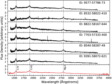
Figure 6.— The six quasar spectra shown in black clustered together in redshift bin $1.57<z<1.8$. The first panel shows the archetype spectrum. The resulting composite spectrum for the cluster is shown in red in the bottom panel.

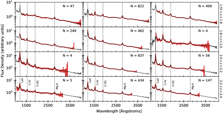
Figure 7.— Three randomly selected composite quasar spectra from each redshift bin are shown in red. The number of quasars in the cluster is noted as N. Overlaid in black is the fit from the 6-vector model described in Section 4.2 and its extrapolation (Section 4.5) beyond the observed wavelength range.

One cluster composite spectrum had strong Mg ii absorption features superimposed on the emission line, resulting in a poor Gaussian fit. In this case, negative features in the continuum-subtracted flux were masked and the line was refit. This masking provided a substantially better estimate for the line location as verified by visual inspection.

The compression of clusters results in a library containing 684 high S/N composite quasar spectra (see Table 2). Six quasar spectra that clustered together in the redshift bin $1.57<z<1.8$ are shown in Figure 6, along with the resulting composite spectrum. The spectra of this cluster all exhibit an apparent break in the continuum around the C iv emission line, demonstrating the ability of the clustering technique to isolate trends in spectral diversity. A randomly selected sample of composite quasar spectra from each redshift bin is shown in Figure 7.

4. Principal Component Analysis

We next create a spectral model to reconstruct the diversity observed in the composite quasar spectra library. In this section, we present the eigenspectra derived from the library and determine the number of eigenspectra necessary to sufficiently model the standard test sample of spectra. We then compare the modeling performance of the eigenspectra to that of the B12 eigenspectra on the standard test sample, BAL test sample, and cluster outliers.

4.1. Eigenspectra

We use Weighted Expectation Maximization Principal Component Analysis (EMPCA; Bailey, 2012) to derive eigenspectra from the composite quasar spectra library. EMPCA was designed to perform PCA on data sets with noise or gaps. Sources of noise in the composite quasar spectra library include composites from clusters with small membership and the extrema of the wavelength range in each composite. Examples of variation in the noise levels can be seen in Figure 7.

The error on each co-added flux measurement was preserved when constructing the composite spectra. These errors are used to weight the flux measurements in each spectrum. The regions of each spectrum with missing data over the rest-frame wavelength range $1060-4023$Å are given weights of zero. The error-weighted mean spectrum of the full library is subtracted from each spectrum to maximize the variance coverage of the first eigenspectrum. Wavelength columns below a minimum data requirement of $5\times N$ nonzero weight values are removed, where N is the number of eigenspectra. We retain nine eigenspectra, covering $1067-4007$ Å, and neglect subsequent eigenspectra.

The mean spectrum and first nine eigenspectra are shown in Figure 8. The four B12 eigenspectra are shown in red for comparison. The spacing between pixels in both eigenspectra sets is uniform in log wavelength at $10^{-4}$. The mean spectrum resembles the first B12 eigenspectrum that was derived without an initial mean subtraction. There is also a noticeable reduction in noise for the eigenspectra of this work relative to the B12 eigenspectra. The B12 eigenspectra are derived from 568 individual quasar spectra, leading to a lower effective S/N.

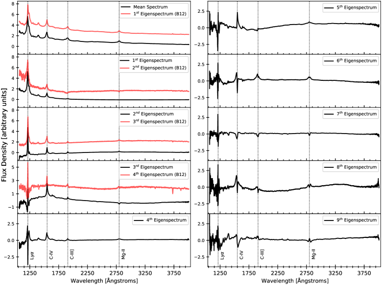
Figure 8.— The mean quasar spectrum and the first nine eigenspectra derived in this work are shown in black. The B12 eigenspectra are shown in red and are offset by two flux units for illustrative purposes.

The eigenspectra of this work capture two notable properties of the C iv emission line: an asymmetry in the C iv line profile and a shift in the line center. The peak of C iv is often significantly blueshifted from the systemic redshift of the quasar, thought to be a result of high-velocity outflows in the broad-line region (e.g. Richards et al., 2011; Shen et al., 2016). The asymmetry is subtle in the first four eigenspectra and becomes more pronounced in the higher-order eigenspectra. A profile asymmetry and line center shift can also be seen in the C iii] emission line in the fifth through eighth eigenspectrum. The ninth eigenspectrum shows significant noise between the Ly$\alpha$ and C iii] emission lines, a region of particular importance for modeling high redshift quasars.

4.2. Modeling the Standard Test Sample

We use the standard test sample of 26,498 quasars to determine the number of eigenspectra required to adequately model the data. Redrock is used to fit the spectra with eigenspectra bases consisting of the mean and the first N eigenspectra, varying N from 3 to 7. Redrock is used in the same configuration to model these spectra using the B12 eigenspectra. Redrock searches over a specified trial redshift range and determines the redshift at which a linear combination of the input eigenspectra best describes an observed spectrum. Redrock also returns the error on the redshift estimate, the coefficients of the eigenspectra in the best fit, the $\chi^{2}$ of the fit, and the $\Delta\chi^{2}$ to the next best fit redshift. This last parameter is the absolute difference in $\chi^{2}$ between the best fit model at the best fit redshift and the best fit model at the second best fit redshift. Larger $\Delta\chi^{2}$ values indicate a higher likelihood that the best fit estimate is correct. We define the trial redshift range for the test samples as $1.6167<z<2.3234$, determined by the redshift coverage of our eigenspectra. These redshift bounds permit a shift as large as $\Delta z=\pm 0.0333$ from the Z_PCA redshifts that lie at the extrema of the test sample redshift range.

The number of eigenspectra retained for final modeling should improve the quality of fit without providing excessive flexibility that limits the ability to differentiate between redshift estimates. For comparison, Z_PCA uses a seven-parameter model consisting of the four B12 eigenspectra plus a quadratic polynomial in $\log\lambda$ to absorb unmodeled broadband signal. We select an eigenspectrum basis consisting of the mean spectrum plus the first five eigenspectra shown in Figure 8, hereafter referred to as the 6-vector model. Increasing the number of eigenspectra in the basis by 1 offers only a 1.7% improvement on the median $\chi^{2}$ of the best fits. More importantly, the inclusion of additional eigenspectra suppresses the distribution of $\Delta\chi^{2}$ to lower values. The medians of the reduced $\Delta\chi^{2}$ distributions for a 5-, 6-, and 7-vector model are 1.440, 1.335, and 1.120, respectively. The 16% reduction from the 6-vector to 7-vector model is indicative of a poorer ability to distinguish between redshifts.

Table 3Percentiles of the reduced $\chi^{2}$ distributions for the B12 and 6-vector models on the unaltered spectra of the standard test sample and after various corrections are applied

		B12			6-vector
	50th	75th	90th	50th	75th	90th
No corrections	1.063	1.254	1.554	0.972	1.099	1.301
Polynomial terms	1.005	1.155	1.385	0.945	1.062	1.255
Extinction corrected	1.061	1.252	1.545	0.972	1.099	1.300
NALs filtered	1.049	1.231	1.509	0.959	1.079	1.263
Extinction corrected and NALs filtered	1.047	1.231	1.501	0.959	1.079	1.262

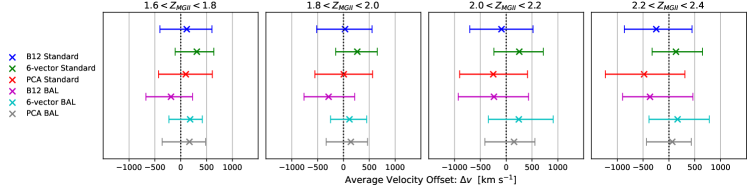
Figure 9.— The average and range of the 16th to 84th percentiles of velocity offset for each redshift bin. The velocity offsets of the B12, 6-vector, and PCA redshifts from Z_MGII are shown. The difference between the B12 model and PCA offsets is primarily a result of masking the Ly$\alpha$ forest.

We compare the performance of the 6-vector model to that of the B12 eigenspectra on the standard test sample. We evaluate the redshift estimates, the resulting reduced $\chi^{2}$ distributions, and reduced $\Delta\chi^{2}$ distributions from both models. The best fits and redshift estimates derived from the B12 eigenspectra in this work differ from Z_PCA in a few key ways: we mask pixels blueward of 1216 Å in the rest frame as determined from Z_PCA during fitting rather than correcting for optical depth, we do not include a quadratic polynomial or apply extinction corrections to the spectra (we devote Section 4.2.1 to testing these corrections), and the redshift search window is inclusive of the range about a spectrum’s Z_PCA estimate but limited to the wavelength coverage of the 6-vector model eigenspectra. For the complete description of Z_PCA, we refer the reader to Section 4.4 of Lyke et al. (2020). We reject 21 spectra that achieved the best fit at the bounds of the trial redshift range for either the B12 or 6-vector model from all further analyses. These objects are primarily misclassified stars, galaxies, or quasars with a true redshift value outside the specified search range.

The redshift estimates from the B12 and 6-vector models are cross-checked against Z_MGII, the redshift of the Mg ii emission line listed in DR16Q. We also compare Z_PCA and Z_MGII. Spectra that have a warning flag associated with Z_MGII are omitted. The velocity offset of the estimated redshift ($Z_{EST}$) from the B12 model, 6-vector model, and Z_PCA relative to Z_MGII is determined as

$$\Delta v=c\times\frac{Z_{EST}-Z_{MGII}}{1+Z_{MGII}}$$ (2)

The standard test sample is split on Z_MGII into four bins of width $\Delta z=0.2$. The average velocity offsets in each bin are shown in Figure 9 along with the corresponding 68% confidence intervals. The 6-vector model displays a consistent, positive average velocity offset across all redshifts. The observed offset for 6-vector redshifts might be a result of modeling choice. We treat the Mg ii emission line as Gaussian when correcting the composite spectra to the proper rest-frame wavelengths. The Z_MGII redshifts are determined using the location of peak flux from PCA fits limited to the vicinity of the Mg ii line.

The average velocity offset across all redshift bins ranges from 136 to 312 km s^-1 for the 6-vector model and from $-$245 to 117 km s^-1 for the B12 model. The average redshift estimates from the B12 model are more consistent with Z_MGII than the 6-vector model estimates in the three lower redshift bins but, similar to Z_PCA, trend lower with redshift and exhibit greater scatter about the average at all redshifts. The average confidence interval has a width of 869 km s^-1 for the 6-vector model and 1144 km s^-1 for the B12 model.

The coefficients of the 6-vector model eigenspectra display one notable trend with absolute velocity offset from Z_MGII. The coefficients of the second eigenspectrum become more negative, while the coefficients of the fifth eigenspectrum trend positive with increasing offset. This trend may be related to the blueshifting of high-ionization emission lines. The greater flux density in these lines relative to the more stable Mg ii line tends to control PCA fits when present. As these lines shift from the systemic redshift, the second eigenspectrum, dominated by narrow line cores, reduces flux at the line centers. Meanwhile, the fifth eigenspectrum, clearly linked to red-blue asymmetry in the C iv and C iii line profiles, acts to correct the shape of the lines, possibly in combination with other eigenspectra.

There are 14 instances where the redshift estimates from the B12 and 6-vector models differ by $\Delta v>10,000$ km s^-1. We visually inspect the spectra to identify the source of tension. Eight of these instances are misclassified stellar spectra or quasar spectra with unidentified BALs. The 6-vector model is consistent with the visual inspection redshift in two cases, and the B12 model is consistent with the visual inspection redshift in three cases. There is one instance were both models failed to accurately estimate the redshift. In addition to the B12 and 6-vector model redshift disagreements, there are 13 spectra with redshift disagreements between the 6-vector model and Z_PCA of $\Delta v>10,000$ km s^-1. These spectra include the three cases where the B12 model correctly estimates the redshift and seven of the misclassified spectra discussed previously. For the remaining three spectra, one is a misclassified nonquasar spectrum, one has an incorrect redshift from both the 6-vector model and Z_PCA, and one has a correct Z_PCA redshift estimate but incorrect 6-vector model redshift.

The distributions of reduced $\chi^{2}$ and reduced $\Delta\chi^{2}$ from the B12 and 6-vector models are shown in Figure 10. The 50th, 75th, and 90th percentiles of the reduced $\chi^{2}$ distributions from each model are given in the first row of Table 3. The more compact reduced $\chi^{2}$ and reduced $\Delta\chi^{2}$ distributions from the 6-vector model relative to the B12 model imply that the 6-vector model provides a better fit to the observed data, but the B12 model is more confident in the redshift estimate, on average. A reduced $\Delta\chi^{2}$ of less than 0.01 is considered the threshold for a poorly determined redshift. Applying this threshold to the reduced $\Delta\chi^{2}$ distributions, we find that 0.72% of redshifts from the B12 model are poorly determined, compared to 0.45% from the 6-vector model.

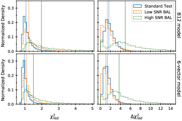
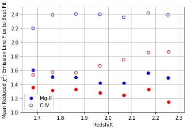
Figure 10.— Top: the distributions of reduced $\chi^{2}$ for the best fits to the spectra of the standard test sample and BAL test sample using the B12 (upper left) and 6-vector (lower left) models, and the corresponding distributions of reduced $\Delta\chi^{2}$ for the B12 (upper right) and 6-vector (lower right) models. In all panels, the BAL test sample is split into two subsamples at an average S/N per pixel of 10. The vertical lines are the median value of each distribution. Bottom: the reduced $\chi^{2}$ of the best fits from the B12 (blue) and 6-vector (red) models in the region of the Mg ii emission line and C iv emission line in the standard test sample as a function of redshift. The uncertainties on the average reduced $\chi^{2}$ are on the 1% level and omitted for clarity.

The composite quasar spectra library was built using the assumption that the location of Mg ii emission line is the least biased from the systemic redshift. We therefore investigate the modeling performance specifically in the Mg ii emission line region. Using the best fits to the full spectrum for the B12 and 6-vector models, we determine the reduced $\chi^{2}$ over the range $2750-2850$ Å for spectra with 50 or more good pixels in this range. The results are shown in Figure 10. The 6-vector model provides lower $\chi^{2}$ fits to the Mg ii region, at 9% on average, across the entire redshift range.

We repeat the above procedure for the C iv emission line region over the wavelength range of $1500-1600$ Å. The results are also shown in Figure 10. The difference in reduced $\chi^{2}$ between the models is more pronounced in the C iv region. Visual inspection reveals that the B12 model is frequently underestimating the peak flux measurements of the C iv emission line. We prioritize the information contained in emission line regions in our clustering analysis, placing emphasis on capturing the range of diversity. Additionally, we are able to expand the basis to six spectral templates instead of four owing to the high S/N of our sample. Both of these factors facilitate reconstruction of the emission line diversity. The trend of increasing reduced $\chi^{2}$ in the C iv region with redshift for the 6-vector model is likely due to the presence of the Ly$\alpha$ emission line influencing the overall fit to quasar spectra with $z>2$.

4.2.1 Additional Modeling Tests

In the previous subsection, we simply modeled the processed spectra with linear combinations of the eigenspectra, excluding flux measurements in the Ly$\alpha$ forest. We now explore the various corrections that were applied to the training sample to assess potential benefits to spectral modeling with the B12 and 6-vector models. We evaluate how correcting for galactic extinction, filtering NALs, and including a quadratic polynomial in $\lambda$ in the fit to absorb broadband signal affect the quality of the best fits on the standard test sample.

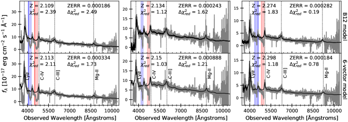
Figure 11.— Each column shows the observer-frame spectrum of a randomly selected BAL quasar in gray. The fits from the B12 (top) and 6-vector (bottom) models are overlaid on the observed spectrum in black. The red and blue shaded regions indicate the masked C iv and Si iv BAL troughs, respectively, as recorded in the BAL Quasar Catalog. The spectra have a BAL_PROB of at least 0.9.

Table 3 quantifies the reduced $\chi^{2}$ distributions of the spectral fits from the B12 and 6-vector models when the corrections to the spectra are applied. The row for “No Corrections” corresponds to the initial best fits. Both models are minimally effected by extinction correction and filtering NALs. The NAL filter simply removes outlier pixels from each spectrum, so both models experience comparable gains. The B12 model benefits significantly from the addition of the quadratic polynomial, while the 6-vector model achieves at most a 4% improvement for any of the corrections. In all iterations, the 6-vector model achieves smaller reduced $\chi^{2}$ values than the B12 model at each percentile. All further modeling is performed without the additional corrections or polynomial tested in this section.

4.3. Modeling the BAL Test Sample

We next evaluate the ability of the 6-vector model and B12 model to fit the quasar spectra in the BAL test sample. We reject the spectra for which Redrock achieves the best fit at the redshift bounds for at least one of the models from all further analyses.

Figure 11 shows three randomly selected BAL quasar spectra and the best fits from the B12 and 6-vector models. The selected quasars all have a BAL_PROB of greater than 0.9. The regions identified in the BAL Quasar Catalog as contaminated with C iv or Si iv associated BALs are indicated in the figure. Both models adequately fit the unabsorbed regions of each spectrum.

We split the BAL test sample on average S/N per pixel at a value of 10, motivated by the S/N limit of the standard test sample. The distribution of the reduced $\chi^{2}$ and reduced $\Delta\chi^{2}$ for the B12 and 6-vector models on the low and high S/N BAL test samples is shown in Figure 10.

The similarity of the reduced $\chi^{2}$ distributions on the low S/N BAL sample and the standard test sample validates our approach to masking the absorption features and supports that BAL and non-BAL quasars are not distinct objects (consistent with Rankine et al., 2020). The reduced $\chi^{2}$ distribution for both models on the high S/N BAL test sample, however, trends toward higher values, with medians of 1.980 and 1.507 for the B12 and 6-vector model, respectively. BALs can be associated with several different emission lines, yet we only mask the most commonly observed BALs associated with C iv and Si iv. The high S/N spectra will suffer a larger penalty than low S/N spectra in the $\chi^{2}$ statistic by not properly modeling other BAL features, if present. In addition, it is impossible to perfectly identify and mask all the C iv and Si iv BAL features that occur; thus, some will unavoidably slip by the masks.

The distribution of $\Delta\chi^{2}$ for the low S/N BAL test sample resembles that for the standard test sample for both the B12 and 6-vector models. As with the standard test sample, the B12 model typically achieves larger $\Delta\chi^{2}$ values for both BAL test samples relative to the 6-vector model. The high S/N sample has a bimodal distribution with a first peak near zero for both models. Applying the threshold of reduced $\Delta\chi^{2}<0.01$ for poorly determined redshift, 0.79% and 0.73% of redshifts are poorly determined from the 6-vector and B12 models, respectively, for the entire BAL sample.

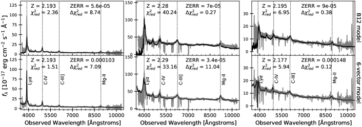
Figure 12.— Each column shows the observer-frame spectrum of a randomly selected cluster outlier in gray. The fits from the B12 (top) and 6-vector (bottom) models are overlaid on the observed spectrum in black.

Following the same procedure as with the standard test sample, the redshift estimates from the B12 model, the 6-vector model, and Z_PCA are checked against Z_MGII. The results are shown in Figure 9. As with the standard test sample, the average offsets from the 6-vector model are consistently positive, show less redshift dependence, and have smaller confidence intervals compared to the B12 model across all bins. The average velocity offset ranges from 117 to 244 km s^-1 for the 6-vector model and from -366 to -188 km s^-1 for the B12 model, with average confidence interval widths of 916 and 1158 km s^-1, respectively. The B12 and 6-vector models show more scatter in the redshift estimates for BAL quasars at high redshifts compared to non-BAL quasars as indicated by the size of the confidence intervals for the two highest redshift bins.

There are 60 spectra with redshift estimates from the B12 and 6-vector models that differ by more than 10,000 km s^-1. We visually inspect these spectra and find that the 6-vector model correctly estimates the redshift in 18 cases, the B12 model correctly estimates the redshift in 11 cases, and both models fail to estimate the redshift in 13 cases. For the spectra where the B12 model redshift is correct, the 6-vector model most often inverts one or more emission lines to match an unmasked BAL feature. For the spectra where the 6-vector model redshift is correct, the B12 model most often exhibits line confusion, matching the template C iv and C iii] emission lines to the true Ly$\alpha$ and C iv flux. Additionally, there are 10 instances of misclassified galaxies, stars, and low redshift quasars. The remaining eight spectra are FeLoBAL quasars, a rare class of spectra exhibiting BALs from low-ionization species including Fe ii and Fe iii (Hall et al., 2002).

4.4. Modeling the Cluster Outliers

We assess the ability of the B12 and 6-vector models to fit more peculiar spectra by fitting a selection of the cluster outlier spectra described in Section 3.2.3. Of the 403 outliers, 271 cluster outliers confirmed as quasars within the redshift range of the standard test sample ($1.65<z<2.29$) are modeled. One quasar spectrum in this sample has an underestimated Z_PCA redshift with a true value beyond the search window and is excluded.

Three cluster outlier spectra and the best fits from the B12 and 6-vector models are shown in Figure 12. While the reduced $\chi^{2}$ values are large compared to the standard test sample, both models provide a qualitatively good fit to the data and are consistent in redshift estimate.

The distributions of reduced $\chi^{2}$ are generally degraded relative to the standard test sample, with median values of 4.871 and 3.480 for the B12 and 6-vector model, respectively. The majority of the modeled outlier spectra contain excessive, unmasked NALs or strong intrinsic absorption features. In nearly all these cases, the best fit from both models describes the observed data well and provides accurate redshift estimates verified by visual inspection. The higher reduced $\chi^{2}$ distributions relative to the standard test sample likely result from the same absorption features that caused the spectra to be rejected as outliers. We note only one redshift failure for these types of outlier spectra in which the 6-vector model inverts an emission feature to match observed absorption in the spectrum. For spectra with strong intrinsic absorption or NALs superimposed on the Ly$\alpha$ emission line, there is a notable trend of the fourth and fifth eigenspectra of the 6-vector model becoming more dominant. The increased contribution of these eigenspectra in the best fit is evident as a sharp decrement in flux at the Ly$\alpha$ line center and asymmetry in the C iv line profile of the fit that is not apparent in the observed spectrum (e.g. third column of Figure 12). The deep flux decrement at the Ly$\alpha$ line center in the fourth and fifth eigenspectra results from strong intrinsic absorption features in a few of the composite spectra from which the principal components were derived. For future studies, a mask may need to be applied to the composite spectra at the location of these strong absorption features to prevent nonphysicality in modeling.

In Section 3.2.3, we identified a broad category of outliers with peculiar spectral features. Most outlier spectra identified as peculiar have atypical emission line flux ratios, continuum slopes, or breaks in spectral index. Both models unambiguously provide accurate redshifts and qualitatively good fits for these spectra. The B12 model often underestimates the emission line flux for Ly$\alpha$, Si iv, C iv, and C iii] across the full outlier sample and in spectra with extreme line ratios (see, e.g., first column of Figure 12). In spectra with a particularly strong and narrow Ly$\alpha$ emission line, the 6-vector model also often falls short in estimating the peak flux. As for spectra with a break in spectral index, the 6-vector model captures the continuum flux more accurately in the far red than does the B12 model.

In addition to the peculiar spectra discussed above, we find a small subset of spectra with unidentified C iv and Si iv BALs and one FeLoBAL spectrum. The results for spectra with unidentified C iv and Si iv BALs are mixed for both models. We do not discuss these further, as the previous section provides a detailed discussion on modeling the spectra of high ionization BAL quasars. For the FeLoBAL spectrum, both models provide accurate redshift estimates, but the continuum fits are influenced heavily by the presence of absorption.

Lastly, there are three peculiar outlier quasars with extremely reddened spectra where the redshift is difficult to estimate. Both models fit one spectrum with clear C iv, C iii], and Mg ii emission lines surprisingly well with accurate redshift estimates. We do not evaluate the best fits to the other two dust-reddened spectra owing to uncertainty in the true redshift. In future implementation of this modeling method, we will consider supplementing the templates to better inform the fitting of dust-reddened quasars.

4.5. PCA Extrapolation and Archetypes

Through fitting an observed spectrum with a linear combination of eigenspectra, we can extrapolate beyond the observed wavelength bounds to the full wavelength range of the PCA model. We fit the spectra of the composite library with the 6-vector model and use the best fits to predict each spectrum’s behavior over the wavelength coverage of the eigenspectra. We show the best fits and extrapolation from the 6-vector model to a random selection of composite spectra in Figure 7.

The models derived from the composite quasar spectra library adequately capture the range of intrinsic diversity in the test samples; therefore, we suggest that the set of extended PCA model spectra from the composite quasar spectra library are accurate representations of quasar spectral diversity. The extended models can be interpreted as essentially noiseless, data-driven archetypes.

There are many potential applications for a quasar archetype library. In particular, if the redshift range for this study is expanded, the archetypes could inform studies of the Ly$\alpha$ forest. It may be feasible to predict the unabsorbed flux in regions contaminated by the forest through matching an observed spectrum to an archetype. Alternatively, measuring the fraction of quasars represented by a given archetype as a function of redshift can provide information on the redshift evolution of quasars.

5. Discussion

We performed a clustering analysis on 12,968 quasar spectra in the redshift range of $1.57<z<2.4$, compressing the sample by nearly a factor of 12. We first determined archetype spectra that are representative of the entire quasar sample. We then identified clusters of quasar spectra, each centered on an archetype spectrum, that are similar on the level of individual flux densities. We implemented three modifications specific to the peculiarities of a large quasar sample. We removed foreground absorption features from the spectra. We reduced the effect of broadband signal in the distance measurement assuming a power law. Lastly, we focused comparisons on the spectral regions that display the most variation, primarily prominent emission lines. We label individual spectra that could not be assigned to any cluster as outliers. We then constructed a library of high S/N composite quasar spectra from the clusters. Including the outliers, our final, compressed sample contains 684 composite quasar spectra, 5 clusters of misclassified stars, 1 misclassified galaxy spectrum, 6 quasar spectra with incorrect redshift estimates resulting from line confusion in PCA, and 396 quasar spectra that are unlike the rest of the sample for varying reasons.

We tested whether the library is representative of the spectral diversity over the sampled redshift range by developing a spectral model through PCA. Our model, the 6-vector model, consists of the mean spectrum of the composite quasar spectra library and the first five eigenspectra. We fit three independent test samples with the 6-vector model: a standard sample of non-BAL quasar spectra, a BAL quasar spectra sample with identified C iv and Si iv BAL features masked, and a selection of outlier spectra from the clustering analysis. All samples were restricted to the redshift range of $1.65<z<2.29$ to permit a free redshift parameter in modeling. The best fits from the 6-vector model were compared to the best fits from the B12 eigenspectra. The results are summarized as follows:

• The 6-vector model achieves an 8.5% reduction in median $\chi^{2}$ on the standard test sample relative to the B12 model. The 6-vector model shows significant improvement in the tail of the reduced $\chi^{2}$ distribution for all samples (see Table 3).

• On average, the B12 model achieves higher values of $\Delta\chi^{2}$ than the 6-vector model, indicative of stronger discrimination between competing redshift estimates. We find that 0.72% of B12 redshift estimates and 0.45% of 6-vector redshift estimates fail to meet the threshold of $\Delta\chi^{2}>0.01$ for the standard test sample. The percentages of poorly determined redshifts on the BAL test sample are roughly equal for both models.

• Both the B12 and 6-vector models attain best fit statistics on the BAL test sample that are comparable to the standard test sample over the same range of S/N. These results support the theory that BAL quasars are not distinct objects and that they display the same range of intrinsic variation in the unabsorbed regions of their spectra as non-BAL quasars.

• Both the B12 and 6-vector models achieve redshift estimates consistent with the redshift of the Mg ii emission line. The B12 model shows stronger average consistency with the Mg ii redshift at lower redshifts but less self-consistency and greater redshift-dependent bias than the 6-vector model across all redshifts.

• The 6-vector model provides higher quality fits to the regions of the C iv and Mg ii emission lines than the B12 model, as shown in Figure 10. The B12 model often underestimates C iv emission line flux, revealed by visual inspection.

• Both models provide good redshift estimates and qualitatively good descriptions of the spectra in the outlier sample. The 6-vector model appears more equipped to model the flux in spectra with extreme emission line ratios. However, there is an unphysical trend in the 6-vector model that leads to occasionally sharp flux decrements on the Ly$\alpha$ emission line. The sharp feature appears in the fourth and fifth eigenspectra as shown in Figure 8.

Several factors contribute to the enhanced performance of the 6-vector model relative to B12. The PCA training sample is constructed to capture the range of population characteristics, primarily in emission line regions, while rejecting contaminants such as misclassified objects. This focus better equips the model to handle atypical emission line fluxes and ratios, as noted in the last bullet point. Further, the high S/N of the sample allowed for correcting all composite spectra to the proper rest frame of the Mg ii emission line through direct fitting of the line. This correction leads to the significant reduction in redshift-dependent bias when redshifting spectra with the 6-vector model. Of equal importance to the previous factors listed, we use 20 times more quasars than the B12 sample, producing eigenspectra with significantly less noise. The noise levels permit retention of higher-order eigenspectra for fitting.

We now summarize some improvements that could further optimize the performance of this technique. First, a more rigorous NAL filter should reduce the number of quasar spectra that are rejected as outliers. A secondary absorption line filter could be applied to the composite quasar spectra library as well, potentially reducing the nonphysical trends we observe in the higher-order eigenspectra. Lastly, we used the propagated error on the composite spectra as weights in EMPCA. We may adjust this approach to increase representation of the smaller clusters and improve modeling of more rare objects.

In the next stages of this study, we will expand the redshift range using the data from the first few months of DESI observations. We echo the sentiments of Yip et al. (2004) that multiple eigenspectra sets, each spanning separate redshift ranges, will improve modeling. Eigenspectra sets covering a specific redshift range can be tuned to the relevant features, consequently providing a proper description of the spectral diversity and allowing for redshift evolution. A natural choice for a split in eigenspectra set is $z\approx 1.5$, below which BALs cannot be automatically detected owing to the absence of the C iv line. BAL diversity could be folded into clustering at low redshifts, allowing spectral templates the flexibility to model these features. Systemic redshifts can be trained on [O ii] and Mg ii for the low and high redshift templates, respectively. Deriving independent spectral models for these two redshift ranges will also allow us to properly capture the spectral diversity arising from galaxy features in the low redshift sample and from the most luminous quasars in the high redshift sample. This new series of spectral models could reduce systematic errors in redshift estimates, mitigate the impact of BALs, and improve predictions of the Ly$\alpha$ forest continuum, thus leading to improved measurements of the baryon acoustic oscillation feature and redshift space distortion with the DESI quasar sample.

References

- Abolfathi et al. (2018) Abolfathi, B., Aguado, D. S., Aguilar, G., et al. 2018, ApJS, 235, 42, doi: 10.3847/1538-4365/aa9e8a
- Ahumada et al. (2020) Ahumada, R., Prieto, C. A., Almeida, A., et al. 2020, ApJS, 249, 3, doi: 10.3847/1538-4365/ab929e
- Alam et al. (2021) Alam, S., Aubert, M., Avila, S., et al. 2021, Phys. Rev. D, 103, 083533, doi: 10.1103/PhysRevD.103.083533
- Bailey (2012) Bailey, S. 2012, PASP, 124, 1015, doi: 10.1086/668105
- Baldwin (1977) Baldwin, J. A. 1977, ApJ, 214, 679, doi: 10.1086/155294
- Blanton et al. (2017) Blanton, M. R., Bershady, M. A., Abolfathi, B., et al. 2017, AJ, 154, 28, doi: 10.3847/1538-3881/aa7567
- Bolton et al. (2012) Bolton, A. S., Schlegel, D. J., Aubourg, É., et al. 2012, AJ, 144, 144, doi: 10.1088/0004-6256/144/5/144
- Boroson (2002) Boroson, T. A. 2002, ApJ, 565, 78, doi: 10.1086/324486
- Boroson & Green (1992) Boroson, T. A., & Green, R. F. 1992, ApJS, 80, 109, doi: 10.1086/191661
- Davies et al. (2018) Davies, F. B., Hennawi, J. F., Bañados, E., et al. 2018, ApJ, 864, 143, doi: 10.3847/1538-4357/aad7f8
- Dawson et al. (2013) Dawson, K. S., Schlegel, D. J., Ahn, C. P., et al. 2013, AJ, 145, 10, doi: 10.1088/0004-6256/145/1/10
- Dawson et al. (2016) Dawson, K. S., Kneib, J.-P., Percival, W. J., et al. 2016, AJ, 151, 44, doi: 10.3847/0004-6256/151/2/44
- DESI Collaboration et al. (2016a) DESI Collaboration, Aghamousa, A., Aguilar, J., et al. 2016a, arXiv e-prints, arXiv:1611.00036. https://arxiv.org/abs/1611.00036
- DESI Collaboration et al. (2016b) —. 2016b, arXiv e-prints, arXiv:1611.00037. https://arxiv.org/abs/1611.00037
- Dey et al. (2019) Dey, A., Schlegel, D. J., Lang, D., et al. 2019, AJ, 157, 168, doi: 10.3847/1538-3881/ab089d
- du Mas des Bourboux et al. (2020) du Mas des Bourboux, H., Rich, J., Font-Ribera, A., et al. 2020, ApJ, 901, 153, doi: 10.3847/1538-4357/abb085
- Dyer et al. (2019) Dyer, J. C., Dawson, K. S., du Mas des Bourboux, H., et al. 2019, ApJ, 880, 78, doi: 10.3847/1538-4357/ab288c
- Fitzpatrick (1999) Fitzpatrick, E. L. 1999, PASP, 111, 63, doi: 10.1086/316293
- Francis et al. (1992) Francis, P. J., Hewett, P. C., Foltz, C. B., & Chaffee, F. H. 1992, ApJ, 398, 476, doi: 10.1086/171870
- Francis et al. (1991) Francis, P. J., Hewett, P. C., Foltz, C. B., et al. 1991, ApJ, 373, 465, doi: 10.1086/170066
- Gunn et al. (2006) Gunn, J. E., Siegmund, W. A., Mannery, E. J., et al. 2006, AJ, 131, 2332, doi: 10.1086/500975
- Guo & Martini (2019) Guo, Z., & Martini, P. 2019, ApJ, 879, 72, doi: 10.3847/1538-4357/ab2590
- Hall et al. (2002) Hall, P. B., Anderson, S. F., Strauss, M. A., et al. 2002, ApJS, 141, 267, doi: 10.1086/340546
- Harris et al. (2016) Harris, D. W., Jensen, T. W., Suzuki, N., et al. 2016, AJ, 151, 155, doi: 10.3847/0004-6256/151/6/155
- Hewett et al. (1995) Hewett, P. C., Foltz, C. B., & Chaffee, F. H. 1995, AJ, 109, 1498, doi: 10.1086/117380
- Hewett & Wild (2010) Hewett, P. C., & Wild, V. 2010, MNRAS, 405, 2302, doi: 10.1111/j.1365-2966.2010.16648.x
- Hou et al. (2021) Hou, J., Sánchez, A. G., Ross, A. J., et al. 2021, MNRAS, 500, 1201, doi: 10.1093/mnras/staa3234
- Jensen et al. (2016) Jensen, T. W., Vivek, M., Dawson, K. S., et al. 2016, ApJ, 833, 199, doi: 10.3847/1538-4357/833/2/199
- Kamble et al. (2020) Kamble, V., Dawson, K., du Mas des Bourboux, H., Bautista, J., & Scheinder, D. P. 2020, ApJ, 892, 70, doi: 10.3847/1538-4357/ab76bd
- Kaspi et al. (2021) Kaspi, S., Brandt, W. N., Maoz, D., et al. 2021, ApJ, 915, 129, doi: 10.3847/1538-4357/ac00aa
- Lundgren et al. (2021) Lundgren, B. F., Creech, S., Brammer, G., et al. 2021, ApJ, 913, 50, doi: 10.3847/1538-4357/abef6a
- Luo et al. (2015) Luo, B., Brandt, W. N., Hall, P. B., et al. 2015, ApJ, 805, 122, doi: 10.1088/0004-637X/805/2/122
- Lyke et al. (2020) Lyke, B. W., Higley, A. N., McLane, J. N., et al. 2020, ApJS, 250, 8, doi: 10.3847/1538-4365/aba623
- Matthews et al. (2020) Matthews, J. H., Knigge, C., Higginbottom, N., et al. 2020, MNRAS, 492, 5540, doi: 10.1093/mnras/staa136
- Myers et al. (2015) Myers, A. D., Palanque-Delabrouille, N., Prakash, A., et al. 2015, ApJS, 221, 27, doi: 10.1088/0067-0049/221/2/27
- Neveux et al. (2020) Neveux, R., Burtin, E., de Mattia, A., et al. 2020, MNRAS, 499, 210, doi: 10.1093/mnras/staa2780
- Pandey (2020) Pandey, B. 2020, MNRAS, 499, L31, doi: 10.1093/mnrasl/slaa152
- Pâris et al. (2011) Pâris, I., Petitjean, P., Rollinde, E., et al. 2011, A&A, 530, A50, doi: 10.1051/0004-6361/201016233
- Pâris et al. (2012) Pâris, I., Petitjean, P., Aubourg, É., et al. 2012, A&A, 548, A66, doi: 10.1051/0004-6361/201220142
- Rankine et al. (2020) Rankine, A. L., Hewett, P. C., Banerji, M., & Richards, G. T. 2020, MNRAS, 492, 4553, doi: 10.1093/mnras/staa130
- Richards et al. (2011) Richards, G. T., Kruczek, N. E., Gallagher, S. C., et al. 2011, AJ, 141, 167, doi: 10.1088/0004-6256/141/5/167
- Rochais et al. (2017) Rochais, T., Singh, V., Chick, W., et al. 2017, MNRAS, 464, 553, doi: 10.1093/mnras/stw2350
- Ross et al. (2012) Ross, N. P., Myers, A. D., Sheldon, E. S., et al. 2012, ApJS, 199, 3, doi: 10.1088/0067-0049/199/1/3
- Ruan et al. (2014) Ruan, J. J., Anderson, S. F., Dexter, J., & Agol, E. 2014, ApJ, 783, 105, doi: 10.1088/0004-637X/783/2/105
- Schlegel et al. (1998) Schlegel, D. J., Finkbeiner, D. P., & Davis, M. 1998, ApJ, 500, 525, doi: 10.1086/305772
- Shang et al. (2003) Shang, Z., Wills, B. J., Robinson, E. L., et al. 2003, ApJ, 586, 52, doi: 10.1086/367638
- Shen & Ho (2014) Shen, Y., & Ho, L. C. 2014, Nature, 513, 210, doi: 10.1038/nature13712
- Shen et al. (2015) Shen, Y., Brandt, W. N., Dawson, K. S., et al. 2015, ApJS, 216, 4, doi: 10.1088/0067-0049/216/1/4
- Shen et al. (2016) Shen, Y., Brandt, W. N., Richards, G. T., et al. 2016, ApJ, 831, 7, doi: 10.3847/0004-637X/831/1/7
- Shields (2007) Shields, J. C. 2007, in Astronomical Society of the Pacific Conference Series, Vol. 373, The Central Engine of Active Galactic Nuclei, ed. L. C. Ho & J. W. Wang, 355. https://arxiv.org/abs/astro-ph/0612613
- Smee et al. (2013) Smee, S. A., Gunn, J. E., Uomoto, A., et al. 2013, AJ, 146, 32, doi: 10.1088/0004-6256/146/2/32
- Suzuki (2006) Suzuki, N. 2006, ApJS, 163, 110, doi: 10.1086/499272
- Suzuki et al. (2005) Suzuki, N., Tytler, D., Kirkman, D., O’Meara, J. M., & Lubin, D. 2005, ApJ, 618, 592, doi: 10.1086/426062
- Tammour et al. (2015) Tammour, A., Gallagher, S. C., & Richards, G. 2015, MNRAS, 448, 3354, doi: 10.1093/mnras/stv126
- Trump et al. (2006) Trump, J. R., Hall, P. B., Reichard, T. A., et al. 2006, ApJS, 165, 1, doi: 10.1086/503834
- Tumlinson et al. (2017) Tumlinson, J., Peeples, M. S., & Werk, J. K. 2017, ARA&A, 55, 389, doi: 10.1146/annurev-astro-091916-055240
- Vanden Berk et al. (2004) Vanden Berk, D., Yip, C., Connolly, A., Jester, S., & Stoughton, C. 2004, in Astronomical Society of the Pacific Conference Series, Vol. 311, AGN Physics with the Sloan Digital Sky Survey, ed. G. T. Richards & P. B. Hall, 21. https://arxiv.org/abs/astro-ph/0310840
- Vanden Berk et al. (2001) Vanden Berk, D. E., Richards, G. T., Bauer, A., et al. 2001, AJ, 122, 549, doi: 10.1086/321167
- Weymann et al. (1991) Weymann, R. J., Morris, S. L., Foltz, C. B., & Hewett, P. C. 1991, ApJ, 373, 23, doi: 10.1086/170020
- Yip et al. (2004) Yip, C. W., Connolly, A. J., Vanden Berk, D. E., et al. 2004, AJ, 128, 2603, doi: 10.1086/425626
- Yu et al. (2021) Yu, Z., Martini, P., Penton, A., et al. 2021, MNRAS, doi: 10.1093/mnras/stab2244
- Zhu (2016) Zhu, G. 2016, arXiv e-prints, arXiv:1606.07156. https://arxiv.org/abs/1606.07156
- Zhu & Ménard (2013) Zhu, G., & Ménard, B. 2013, ApJ, 770, 130, doi: 10.1088/0004-637X/770/2/130
- Zou et al. (2021) Zou, S., Jiang, L., Shen, Y., et al. 2021, ApJ, 906, 32, doi: 10.3847/1538-4357/abc6ff