Asymmetric Graph Representation Learning

Abstract

Despite the enormous success of graph neural networks (GNNs), most existing GNNs can only be applicable to undirected graphs where relationships among connected nodes are two-way symmetric (i.e., information can be passed back and forth). However, there is a vast amount of applications where the information flow is asymmetric, leading to directed graphs where information can only be passed in one direction. For example, a directed edge indicates that the information can only be conveyed forwardly from the start node to the end node, but not backwardly. To accommodate such an asymmetric structure of directed graphs within the framework of GNNs, we propose a simple yet remarkably effective framework for directed graph analysis to incorporate such one-way information passing. We define an incoming embedding and an outgoing embedding for each node to model its sending and receiving features respectively. We further develop two steps in our directed GNN model with the first one to aggregate/update the incoming features of nodes and the second one to aggregate/update the outgoing features. By imposing the two roles for each node, the likelihood of a directed edge can be calculated based on the outgoing embedding of the start node and the incoming embedding of the end node. The log-likelihood of all edges plays a natural role of regularization for the proposed model, which can alleviate the over-smoothing problem of the deep GNNs. Extensive experiments on multiple real-world directed graphs demonstrate outstanding performances of the proposed model in both node-level and graph-level tasks.

1 Introduction

GNNs provide a powerful framework for graph representation learning. One of the main reasons for GNNs’ success is the networks’ capability of generating representations of nodes that actually depend on the structure of the graph, as well as node feature information. Most GNNs belong to one of the two categories: spectral-based networks [4, 6, 13] or spatial-based networks [10, 33, 14]. The spectral-based GNNs use adjacency matrices to explore the neighborhood based on spectral graph theory from the perspective of graph signal processing. The spatial-based approaches, on the other hand, directly perform the convolution in the graph domain by aggregating information of the neighbor nodes. Numerous GNN variants have also been proposed, and most of them can be reformulated into a single common framework [9], called message passing neural networks (MPNNs). These models employ a message passing procedure to aggregate local information of vertices.

Although GNNs have achieved practical successes in many aspects, most of the existing methods only focus on undirected graphs. The directed graphs have been largely ignored or been simplified with undirected settings [10]. However, relationships in directed graphs are asymmetric, which contain essential structural information about the graph. As a special type of graphs, the directed graphs arise broadly across different domains; for instance, the email networks [16], citation networks [28], natural language sentences [35], as well as website networks [39], etc. These examples all involve directional edges, indicating receiving and sending information in one-way or two-way flow among nodes.

In undirected graphs, relationships among nodes are symmetric. Directed graphs, in contrast, have asymmetric node relationships. In particular, some nodes can have edges of both in-taking (receiving information) and out-flowing (sending information) functions, which makes GNNs learn the graph feature much more difficult than the undirected graph setting. It is challenging to model directed graphs using the current framework of GNNs due to the asymmetric structure. How to incorporate directed structural information into the node representation for higher predictive power is an important task. All the aforementioned methods, whether the spectral-based or spatial-based approaches, cannot be directly applied to directed graphs. For spectral-based methods, they are limited to use undirected graphs as input by definition, and the graph Laplacian needs to be symmetric. Therefore, extending spectral methods to directed graphs is not straightforward because the adjacency matrix is asymmetric and there is no obvious way to define a symmetric Laplacian. For spatial-based approaches, there are natural advantages on extension to directional settings, but most of the existing methods [10, 31, 29] are not efficient to capture the complex structure of directed graphs. How to extend GNNs from undirected graphs to directed graphs needs to be further explored.

The existing GNN solutions for directed graphs fall into one of the two categories. A majority of them is to relax directed graphs to undirected ones, i.e., by trivially adding edges to symmetrize the adjacency matrices [17, 29, 16, 28]. The disadvantages of these methods are obvious. Relaxing directional edges to undirected settings would incur loss of information on the asymmetric node relationships, which cannot represent the distinctive directional structure, such as irreversible citations, hyperlinks, mailings, and time-series relationships, etc. For example, in a citation graph, a later published article can cite a previously published article, but not the opposite due to such a unique time-series relationship. If we convert a citation relationship network into an undirected graph, noise or bias would be introduced inevitably. Although we can represent the original directed graph in another form, such as a temporal graph learned by a combination of recurrent neural networks (RNNs) and GNNs [18], we still hope to mine more structural features from the original directed graph without adding additional components. Some other methods [17, 29] have to stipulate learning templates or rules in advance, which is very complicated and difficult to explain, and is not capable of dealing with complex structures beyond their definitions [28].

There are also other works aiming to learn specific directed structures by using the incident matrix with attributes of edges [25, 8], through defining a complex Hermitian matrix known as the magnetic Laplacian, aggregating directed predecessors information [31, 27] and defining a vector field with the eigenvectors of graph Laplacian [1]. In particular, Beani et al. [1] define directed convolution with vector fields on a graph. However, these methods for directed graphs either lack interpretability under the framework of the spectral and spatial graph learning [25, 8, 31, 27] or are faced with scalability problems [1].

Inspired by the co-clustering algorithm for directional community detection [20], we let one node play two different roles in a directed graph, i.e., the incoming-node and outgoing-node, to accommodate the asymmetries of the directed graph. Specifically, within the framework of GNNs, we introduce two types of embedding with an outgoing vector and an incoming vector (of the same dimension), for each node. The incoming embedding aims to capture receiving features and the outgoing embedding aims to capture sending-out features. Figure 1 illustrates an example of such asymmetric node representations, where node $v$ in a directed graph is described by both an incoming vector $\mathbf{r}_{v}$ and an outgoing vector $\mathbf{s}_{v}$. Different from traditional GNNs where each node in an undirected graph is represented as a single vector, the asymmetric structure of the directed graph is characterized by both $\mathbf{r}_{v}$ and $\mathbf{s}_{v}$. The asymmetric node representations facilitate interpretable edge representations as well. Any edge in a directed graph can be characterized by the outgoing embedding of its source node and the incoming embedding of its target node.

Traditionally, within the framework of MPNNs, GNNs can be generalized as one aggregating step and one subsequent updating step. With the asymmetric representations, we extend the traditional GNN framework to the directed graph by defining two aggregating/updating steps, with the first one to aggregate/update the receiving features of nodes and the second one to aggregate/update sending-out features. The asymmetrical property of the proposed GNN makes each node in a directed graph exchange (aggregate/update) “messages” with the neighbors in two different ways: the in-taking information and the out-flowing information. The incoming embedding and outgoing embedding obtained by GNNs can preserve the structural information of the directed graph. Moreover, the likelihood of a directional edge can be modeled by the outgoing embedding of its source node and the incoming embedding of its target node, which is a natural regularization term of the proposed model that can alleviate the issue of over-smoothing. The embeddings of nodes would be similar due to lager receptive fields through message passing as the number of layers increases [34], which is known as over-smoothing problem of GNNs. The proposed regularization term, in contrast, maintains similarity among 1-hop neighbors, which can balance messages over propagation by restraining the receptive field.

The contributions of this work are as follows:

• We propose a novel directed graph neural network, called asymmetric GNN (AGNN), with the incoming and outgoing embeddings to learn the different roles for each node in directed graphs;

• A novel regularization term is proposed to alleviate the over-smoothing issue;

• Our approach works well on different directed graph datasets in semi-supervised nodes classification and graph regression tasks, and achieves better performance than the state-of-the-art directed GNN methods.

The rest of the paper is organized as follows. Section 2 introduces the related work in GNNs. Section 3 formulates the basic GNN models for undirected graphs. The detailed formulation of our proposed AGNN is given in Section 4. The ablation study and comparisons with the state-of-the-art methods are shown in Section 5. Section 6 concludes the paper with remarks.

2 Related Work

2.1 Directed Graph Neural Networks

A majority of GNNs transform directed graphs to undirected ones by relaxing its direction structure, i.e., trivially adding edges to symmetrize the adjacency matrices. Monti, Otness, and Bronstein [17] deal with directed graphs by exploiting local graph motifs [2], which define a new set of symmetric motif adjacency matrices. Tong et al. [29] use first-order and second-order proximity to obtain symmetric adjacency matrices, which not only can retain the connection properties of the directed graph, but also expand the receptive field of the convolution operation. Ma et al. [16] and Tong et al. [28] leverage Perron–Frobenius theorem and the stationary distribution of strongly connected graphs to generalize the Laplacians of undirected graphs to directed graphs. They also eliminate the directed structure to guarantee that the normalized Laplacian is symmetric. Tong et al. [28] further exploit the $k$th-order proximity between two nodes in a digraph by the inception network [26], which not only allows the model to learn features of different sizes within one convolutional layer but also obtains larger receptive fields.

There are several works that learn the specific directed structure. In [25] and [8], the incident matrix is used to combine the attributes of the incoming edges, outgoing edges and vertex itself to update the vertex and combine the attributes of the source nodes, target nodes and edge itself to update the edge. Wang et al. [31] incorporate an attention mechanism to obtain the edge attention matrix or 1-hop attention matrix and further compute the attention scores of multi-hop neighbors via graph diffusion based on the powers of the 1-hop attention matrix and then define the graph attention diffusion based feature aggregation. Zhang et al. [39] encode the undirected geometric structure in the magnitude of its entries and directional information in the phase of its entries based on a complex Hermitian matrix known as the magnetic Laplacian. Thost and Chen [27] use attention mechanism to only aggregate directed predecessors information from the current layer and GRU to combine the neighbor and previous representation. Beani et al. [1] exploit vector flows over graphs to develop a globally consistent directional and asymmetric aggregation function. They define a vector field in the graph by use of the Laplacian eigenvectors and develop a method of applying directional derivatives and smoothing by projecting node-specific messages into the field.

2.2 Over-Smoothing

From the perspective of information propagation, GNNs can be understood as an aggregation of information about neighboring nodes, and then after several GNNs messaging iterations, the representation of all nodes in the graph may become similar. This tendency is particularly common in basic GNN models and some models using self-loop update methods [11]. From the perspective of random wandering, when we use a $K$-layer GNN model, the effect of node $u$ on node $v$ is proportional to the probability of reaching node $v$ with $K$ random wandering steps starting from node $u$ [34]. However, when $K$ is large enough, the impact of each node approaches a smooth distribution of random wanderings on the graph, which means that local information is lost. The embedding of the nodes becomes over-smoothed, approaching an almost uniform distribution [12]. The over-smoothing problem makes it impossible to construct deeper GNN models to exploit long-term dependencies in the graph, as these deep GNN models tend to generate only over-smoothed node embeddings. Some recent works aim to solve this problem. Xu et al. [34] perform concatenation, max-pooling or LSTM-attention operations on the output of each layer to adapt the receptive filed of each node instead of using only the output of the last layer. Klicpera, Bojchevski, and Günnemann [14] use a variant of PageRank, personalized PageRank, considers the root node and preserve the information of the original features to some extent, whose update process is similar to the linear combination of the convolved features with the initial features. Pham et al. [19] and Chen et al. [5] use an approach similar to the residual connectivity in convolutional neural networks (CNNs) to train deeper networks, i.e., the feature representation of a node is a linear interpolation between the previous representation of the node and the representation of neighboring nodes. Li et al. [15] and Selsam et al. [22] use the gated recurrent unit (GRU) and long short-term memory (LSTM) architecture to update the feature representation of the nodes. These strategies are very effective in facilitating deep GNN architectures (e.g., more than 10 layers) and preventing over-smoothing. Rong et al. [21] and Feng et al. [7] use DropEdge and DropNode strategies and a framework for contrast learning, respectively, to address the over-smoothing problem. However, these methods are proposed to address the over-smoothing problem for undirected graph, and there are few approaches for the directed graph.

3 Preliminaries

Let $\mathcal{G=(V,E)}$ be an undirected graph with $n$ nodes, where $\mathcal{V}=\{1,\dots,n\}$ is the set of $n$ nodes, $\mathcal{E\subseteq V\times V}$ is the set of edges connecting paired nodes in $\mathcal{V}$. The graph structure is represented by the $n\times n$ symmetric adjacency matrix $\mathbf{A}=\{a_{ij}\}_{i,j=1}^{n}$, where $a_{ij}=1$ if there exists an edge between nodes $i$ and $j$, and $a_{ij}=0$ otherwise. The degree matrix $\mathbf{D}\in\mathbb{R}^{n\times n}$ is a diagonal matrix, where $\mathbf{D}_{ii}=\sum_{i}a_{ij}=\sum_{j}a_{ij}$. Let $\mathbf{X}\in\mathbb{R}^{n\times d}$ denote the feature matrix of the $n$ nodes if graph $\mathcal{G}$ is associated with attributes. If the node attributes are not given, we can encode nodes as a one-hot vector, that is, $\mathbf{X}=\mathbf{I}$, where $\mathbf{I}\in\mathbb{R}^{n\times n}$ is an identity matrix. GNNs learn node or edge representation vectors by using the graph structure $\mathbf{A}$ and node feature matrix $\mathbf{X}$. To facilitate subsequent discussions, we formalize an $L$-layers GNN under the architecture of MPNNs [9], which computes the $l$-th layer representation vector $\mathbf{h}_{v}^{l}$ for node $v$ in a graph $\mathcal{G}$ as

$$\mathbf{m}_{v}^{l} =\text{AGGREGATE}^{l}\left(\left\{\mathbf{h}_{u}^{l-1}\ |\ u\in\mathcal{N}(v)\right\}\right)$$

$$\mathbf{h}_{v}^{l} =\text{COMBINE}^{l}\left(\mathbf{h}_{v}^{l-1},\mathbf{m}_{v}^{l}\right),\ \ l=1,\dots,L,$$

where $\mathbf{h}_{u}^{0}=\mathbf{X}_{u}$ is the input feature of node $u$, $\mathcal{N}(v)$ is a set of neighbors adjacent to $v$ in the graph. Under the framework of MPNNs, messages flow from $\mathcal{N}(v)$ to $v$ using an aggregation function (AGGREGATE), and then $\mathbf{h}_{v}^{l}$ of node $v$ is updated based on the corresponding neighbor messages $\mathbf{m}_{v}^{l}$ from the previous message aggregation step.

Many existing methods [13, 15, 30, 33] are specific examples of the MPNNs framework and the differences lie in the choices of AGGREGATE and COMBINE functions.

3.1 GCN

In the graph convolutional networks (GCN) [13], initially motivated by spectral graph convolutions [4, 6], the AGGREGATE and COMBINE steps are integrated as follows,

$$\mathbf{h}_{v}^{l}=\text{ReLU}\left(\mathbf{W}\cdot\text{MEAN}\left\{\mathbf{h}_{u}^{l-1},\forall u\in\mathcal{N}(v)\cup\{v\}\right\}\right),$$

where $\mathbf{W}$ is a linear parameter matrix and MEAN represents an element-wise mean pooling.

3.2 GraphSAGE

In the pooling variant of GraphSAGE [10], AGGREGATE and COMBINE are formulated as

$$\mathbf{m}_{v}^{l} =\text{MAX}\left(\left\{\text{ReLU}(\mathbf{W}\cdot\mathbf{h}_{u}^{l-1}),\forall u\in\mathcal{N}(v)\right\}\right)$$

$$\mathbf{h}_{v}^{l} =\mathbf{W}\cdot\left(\mathbf{h}_{v}^{l-1}\parallel\mathbf{m}_{v}^{l}\right),$$

where MAX represents an element-wise max pooling and $\parallel$ denotes the concatenation operation.

For node-level tasks, the node representation $\mathbf{h}_{v}^{L}$ of the final layer $L$ is used for prediction. For graph-level tasks, the READOUT function computes a feature vector for the whole graph using some readout function according to

$$\mathbf{h}_{\mathcal{G}}=\text{READOUT}\left(\left\{h_{v}^{L},v\in\mathcal{V}\right\}\right),$$

where READOUT can be a simple permutation invariant function such as summation or a more sophisticated graph-level pooling function [36, 37].

4 Method

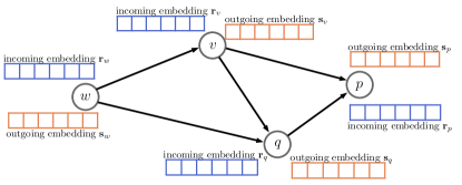
Figure 1: Illustration of the outgoing embedding and the incoming embedding over a four-node toy graph. For example, node $v$ has both the outgoing embedding $\mathbf{s}_{v}$ and incoming embedding $\mathbf{r}_{v}$, which describe the sending and receiving pattern respectively. Node $w$ has two outgoing edges but no incoming edge, hence its incoming embedding $\mathbf{r}_{w}=\mathbf{0}$. Likewise, the outgoing embedding $\mathbf{s}_{p}=\mathbf{0}$ because node $p$ only contains incoming edges. The occurrence of a directional edge can be interpreted by the two types of embedding. For instance, the likelihood of edge $w\to v$ depends on $\mathbf{s}_{w}$ and $\mathbf{r}_{v}$.

Traditionally, in undirected graphs, relationships are symmetric, and thus a node is represented by a single vector embedding $\mathbf{h}$. Directed graphs, in contrast, have asymmetric node relationships. In particular, some nodes can have edges of both in-taking (receiving information) and out-flowing (sending information) functions, which would make GNNs learn the graph representation more difficult than an undirected setting. To capture the asymmetries, we propose to represent node $v$ in a directed graph with an outgoing (sending information) embedding vector $\mathbf{s}_{v}$ and an incoming (receiving information) embedding vector $\mathbf{r}_{v}$, as shown in Figure 1. Based on the two different roles of each node, we develop an asymmetric GNN, which contains two steps with the first one to aggregate/update its incoming features and the second one to aggregate/update its outgoing features.

Formally, given a directed graph $\mathcal{G}=(\mathcal{V},\mathcal{E})$ with $n$ nodes, we have an asymmetric adjacency matrix $\mathbf{A}=\{a_{ij}\}_{i,j=1}^{n}$, where $a_{ij}=1$ if there exists a directed edge pointing from node $i$ to node $j$, and $a_{ij}=0$ otherwise. Specifically, each node can be split into an out-node and an in-node, and the rows of $\mathbf{A}$ index the out-nodes and the columns of $\mathbf{A}$ index the in-nodes. Thus, the directed graph has two diagonal degree matrices: an in-degree matrix $\mathbf{P}\in\mathbb{R}^{n\times n}$ with $\mathbf{P}_{ii}=\sum_{i}^{n}a_{ji}$ and an out-degree matrix $\mathbf{O}\in\mathbb{R}^{n\times n}$ with $\mathbf{O}_{ii}=\sum_{j}^{n}a_{ij}$. Note that the in-degree and out degree of each node are equal in undirected graph, because of the symmetrical $\mathbf{A}$. The nodes are characterized by the feature matrix $\mathbf{X}\in\mathbb{R}^{n\times d}$ which is the same as undirected graphs.

The main idea of asymmetric graph neural network (AGNN) is to process nodes according to the different behaviors in terms of sending and receiving patterns so as to learn receiving and sending feature maps, respectively.

4.1 Asymmetric Message Passing

We develop a multi-layer AGNN with the following rules,

$$\mathbf{m}_{v}^{l} =\text{AGGREGATE}_{1}^{l}\left(\left\{\mathbf{r}_{u}^{l-1}\ |\ u\in\mathcal{N}_{in}(v)\right\}\right)$$ (1)

$$\mathbf{a}_{v}^{l} =\text{AGGREGATE}_{2}^{l}\left(\left\{\mathbf{s}_{w}^{l-1}\ |\ w\in\mathcal{N}_{out}(v)\right\}\right)$$

$$\mathbf{r}_{v}^{l} =\text{COMBINE}_{1}^{l}\left(\mathbf{r}_{v}^{l-1},\mathbf{m}_{v}^{l}\right)$$

$$\mathbf{s}_{v}^{l} =\text{COMBINE}_{2}^{l}\left(\mathbf{s}_{v}^{l-1},\mathbf{a}_{v}^{l}\right),$$

where $\mathbf{r}_{v}^{0}=\mathbf{s}_{v}^{0}=\mathbf{X}_{v}$ is the input feature of $v$, $\mathcal{N}_{in}(v)$ and $\mathcal{N}_{out}(v)$ denote the sets of direct predecessors and successors of $v$ respectively. More specifically, for $\forall u\in\mathcal{V}$, if there exists an edge $u\to v$, then $u\in\mathcal{N}_{in}(v)$; likewise, for $\forall w\in\mathcal{V}$, if there exists an edge $v\to w$, then $w\in\mathcal{N}_{out}(v)$. $l=1,2,\dots,L$ denotes the layer of convolution. Finally, we can model the different roles of receiving and sending information, and obtain two embeddings of one node (i.e., the receiving messages flow from $\mathcal{N}_{in}(v)$ to the incoming embedding $\mathbf{r}_{v}$ and the sending messages flow from $\mathcal{N}_{out}(v)$ to the outgoing embedding $\mathbf{s}_{v}$ for node $v$, respectively).

For node-level tasks, the two node representations $\mathbf{r}_{v}^{L}$ and $\mathbf{s}_{v}^{L}$ of the final layer are merged and used for prediction,

$$\mathbf{z}_{v}=\text{COMBINE}_{3}\left(\mathbf{r}_{v}^{L},\mathbf{s}_{v}^{L}\right),$$ (2)

where $L$ is the number of layers. For graph-level tasks, the readout phase computes a feature vector for the whole graph according to

$$\mathbf{z}_{\mathcal{G}}=\text{READOUT}\left(\{\mathbf{z}_{v},v\in\mathcal{V}\}\right).$$

By defining the specific AGGREGATE and COMBINE functions, we would obtain a corresponding directed GNN method. For instance, consider the element-wise mean pooling in the framework of the asymmetric message passing, it is a directed version of GCN,

$$\mathbf{S}^{l} =\sigma\left(\tilde{\mathbf{A}}\mathbf{S}^{l-1}\mathbf{W}_{1}^{l}\right)$$ (3)

$$\mathbf{R}^{l} =\sigma\left(\hat{\mathbf{A}}\mathbf{R}^{l-1}\mathbf{W}_{2}^{l}\right),$$

where $\mathbf{S}^{0}=\mathbf{R}^{0}=\mathbf{X}\in\mathbf{R}^{n\times d}$, $\sigma$ is an activation function (e.g., ReLU), $\tilde{\mathbf{A}}=\mathbf{O}^{-1/2}(\mathbf{A}+\mathbf{I})\mathbf{P}^{-1/2}\in\mathbb{R}^{n\times n}$ is the normalized adjacency matrix of the directed graph $\mathcal{G}$ with added self-connections, $\hat{\mathbf{A}}=\mathbf{P}^{-1/2}(\mathbf{A}^{T}+\mathbf{I})\mathbf{O}^{-1/2}\in\mathbb{R}^{n\times n}$ and $\mathbf{W}_{1}^{l},\mathbf{W}_{2}^{l}\in\mathbb{R}^{d_{l-1}\times d_{l}}$ are trainable parameters. $\mathbf{S}^{l}$ and $\mathbf{R}^{l}$ are the sending and reveiving embedding of the $l$-th layer in matrix form. Through Eq. (3), we can aggregate (i.e., mean) the predecessor (or successor) and root nodes to matrix $\mathbf{R}^{l}$ (or $\mathbf{S}^{l}$). We let $\mathbf{S}:=\mathbf{S}^{L}$ and $\mathbf{R}:=\mathbf{R}^{L}$ for notation simplicity, where $\mathbf{S}^{L}$ and $\mathbf{R}^{L}$ are the outgoing and incoming embeddings of the $L$-th layer.

For node classification, we can coalesce the incoming and outgoing embedding vectors, followed by a softmax function to map every node to a probability distribution,

$$\mathbf{Z}=\text{Softmax}\left(\mathbf{R}+\mathbf{S}\right).$$

For graph classification, we can concatenate the two embeddings, and a sum pooling is followed to obtain the graph-level representation,

$$\mathbf{Z} =\text{FC}\left(\mathbf{R}\parallel\mathbf{S}\right)\in\mathbb{R}^{n\times d},$$

$$\mathbf{Z}_{\mathcal{G}} =\text{SUM}\left(\mathbf{Z}\right)\in\mathbb{R}^{1\times d},$$

where FC denotes the fully-connected layer and $\parallel$ denotes the concatenate operation.

4.2 Loss Function

4.2.1 Classification Loss

For semi-supervised multi-class classification, we evaluate the cross-entropy error over all labeled examples,

$$\mathcal{L}_{\text{error}}=-\sum_{l\in\mathcal{Y}_{L}}\sum_{c=1}^{C}\mathbf{Y}_{lc}\ln\mathbf{Z}_{lc},$$

where $\mathcal{Y}_{L}$ is the set of node (graph) indices that have labels, $\mathbf{Y}_{lc}$ is the true label, $\mathbf{Z}_{lc}$ is the predicted label and $C$ is the number of classes.

4.2.2 Regularization Formulation.

With the proposed asymmetric node embeddings for directed graphs, the likelihood of a directional edge can be calculated based on the outgoing embedding of its source node and the incoming embedding of its target node. As shown by the example in Figure 1, the occurrence of the edge $v\to q$ can be interpreted together by the vectors $\mathbf{s}_{v}$ and $\mathbf{r}_{q}$. The likelihood of graph $\mathcal{G}$ can be jointly calculated based on the likelihood of edges. A regularization formulation equips the log-likelihood of $\mathcal{G}$ to avoid over-smoothing for the proposed model. As the number of layers increases, the embeddings of nodes may be similar due to lager receptive fields through message passing, while the regularization formulation would maintain the virginity that nodes are similar to their direct neighborhoods. In other words, nodes connected by the same edge preserve similar features.

In particular, considering the outgoing embedding set $\{\mathbf{s}_{i}\}_{i=1}^{n}$ and the incoming embedding set $\{\mathbf{r}_{j}\}_{j=1}^{n}$ for all the nodes, we formulate the likelihood of an edge $i\to j$ with the inner product between $\mathbf{s}_{i}$ and $\mathbf{r}_{j}$ followed by a sigmoid function,

$$p_{ij}=\text{sigmoid}\left(\mathbf{s}_{i}^{T}\mathbf{r}_{j}\right)=\frac{1}{1+\exp(-\mathbf{s}_{i}^{T}\mathbf{r}_{j})},$$

where $p_{ij}=P(a_{ij}=1)$, and $\mathbf{s}_{i}$ is the outgoing embedding of node $i$ and $\mathbf{r}_{j}$ is the incoming embedding of node $j$ obtained from Eq. (1).

Consequently, the likelihood function of $\mathcal{G}$ is

$$P(\mathcal{G})=\prod_{i,j=1}^{n}p_{ij}^{a_{ij}}(1-p_{ij})^{1-a_{ij}}=\prod_{i,j=1}^{n}\frac{\exp(\mathbf{s}_{i}^{T}\mathbf{r}_{j}a_{ij})}{1+\exp(\mathbf{s}_{i}^{T}\mathbf{r}_{j})}.$$

This leads to the negative log-likelihood function (regularization),

$$\mathcal{L}_{\text{reg}}(\mathbf{s},\mathbf{r}) =-\frac{1}{n^{2}}\sum_{i,j=1}^{n}\Big{(}\mathbf{s}_{i}^{T}\mathbf{r}_{j}a_{ij}-\log\big{(}1+\exp(\mathbf{s}_{i}^{T}\mathbf{r}_{j})\big{)}\Big{)}$$

$$=-\frac{1}{n^{2}}\mathbf{1}^{T}\Big{(}\mathbf{S}^{T}\mathbf{R}\odot\mathbf{A}-\log\big{(}1+\exp(\mathbf{S}^{T}\mathbf{R})\big{)}\Big{)}\mathbf{1},$$

where $\mathbf{1}$ denotes the vector with all entries being $1$, $\mathbf{S}$ and $\mathbf{R}$ are given in Eq. (3) and $\odot$ denotes the Hadamard product. Finally, we obtain the total loss function,

$$\mathcal{L}=\mathcal{L}_{\text{error}}+\lambda\mathcal{L}_{\text{reg}},$$ (4)

where $\lambda$ is a hyper-parameter as the regularization coefficient, serving as a trade-off between the classification error and regularization.

Furthermore, the proposed method is very flexible and can be extend to undirected graph by setting $\mathbf{r}_{v}=\mathbf{s}_{v}$ for each node $v$.

5 Experiment

We evaluate the effectiveness of our model on both node-level and graph-level tasks. Node-level experiments are performed on citation and co-purchase datasets, graph-level on a neural architecture dataset. A common task of GNNs is semi-supervised node classification, which can be used to verify the learning capability of our model. Another task is graph regression, which can be used to verify that our model is not node-level-specific and can be easily adapted to graph-level task. Compared with the canonical experiments for undirected graphs, the main difference lies in that the task under our setup is applied to the directed graphs and the given adjacency matrix $\mathbf{A}$ is asymmetric. The Supplementary Material reports details on the experiments and reproducibility.

5.1 Experimental Settings

5.1.1 Datasets.

For semi-supervised node classification task, we apply the AGNN on four directed graph datasets with detailed information given in Table 1. The four real datasets include two citation datasets: Cora-ML [3] and Citeseer [23], and two Amazon co-purchase datasets [24]: AM-Computer and AM-Photo. In our experiments, we randomly split the datasets and perform multiple experiments for obtaining stable and reliable results. The mean and standard deviation of classification accuracy are calculated by running each experiment $20$ times with random weight initialization. For training/validation/testing split, we follow the rules in DiGCN [28] to choose 20 labels per class for the training set, 500 labels for the validation set and the rest for the testing set. For graph regression task, we apply our model on NA dataset [38]. The NA dataset contains 19020 neural architectures from the ENAS software. The task is to evaluate each neural architecture’s weight-sharing accuracy on CIFAR-10 . Since it is a regression task, we use the RMSE, MAE and MAPE metrics. Followed by [27], we randomly split the dataset into 90% training and 10% held-out test sets.

5.1.2 Baselines.

We compare our model with seven state-of-the-art models that can be divided into three main categories: (i) spectral-based GNNs including GCN [13], SGC [32], APPNP [14]; (ii) spatial-based GNNs including GraphSage [10] and GAT [30]; and (iii) directed GNNs including DGCN [29] and DiGCN [28].

5.1.3 Implementation Details.

For citation datasets, Cora-ML and Citeseer, we train our model for a maximum of 1000 epochs with early stopping if the validation accuracy does not increase for 200 consecutive epochs and the hidden layer dimension is 64. For Amazon co-purchase datasets, AM-Computer and AM-Photo, we train our model for a maximum of 500 epochs without early stopping and the hidden layer dimension is 128. In the four node-level datasets, the learning rate is 0.01, the weight decay is 0.0005, and the dropout rate is 0.5. We calculate the mean test accuracy with standard deviation in percent (%) averaged over 20 random dataset splits with random weight initialization. For NA dataset, we train our model for a maximum of 100 epochs and the hidden layer dimension is 64. The learning rate is 0.001, the batch size is 32 and the dropout rate is 0.5.

Datasets	Nodes	Edges	Classes	Features	Label rate
Cora-ML	2995	8416	7	2879	4.67%
Citeseer	3312	4715	6	3703	3.62%
Am-Computer	13752	287209	10	767	1.45%
Am-Photo	7650	143663	8	745	2.10%

Table 1: Detailed information on the four real datasets. We choose 20 labels per class for the training set following DiGCN [28].

5.2 Experimental Results

Models	Cora-ML	Citeseer	Am-Computer	Am-Photo
GCN	53.11 ± 0.8	54.36 ± 0.5	60.50 ± 1.6	53.20 ± 0.4
SGC	51.14 ± 0.6	44.07 ± 3.5	76.17 ± 0.1	71.25 ± 1.3
APPNP	70.07 ± 1.1	65.39 ± 0.9	63.16 ± 1.4	79.37 ± 0.9
GraphSage	72.06 ± 0.9	63.19 ± 0.7	79.29 ± 1.3	87.57 ± 0.9
GAT	71.91 ± 0.9	63.03 ± 0.6	79.45 ± 1.5	89.10 ± 0.7
DGCN	75.02 ± 0.5	66.00 ± 0.4	/	83.66 ± 0.8
DiGCN	80.28 ± 0.5	66.11 ± 0.7	85.94 ± 0.5	90.02 ± 0.5
AGNN w/o reg	80.52 ± 0.3	69.07 ± 0.3	84.27 ± 0.7	90.67 ± 0.3
AGNN w reg	80.76 ± 0.2	69.21 ± 0.3	84.34 ± 0.7	90.70 ± 0.3

Table 2: Overall accuracy comparison on node classification between our AGNN without regularization and AGNN with regularization and seven existing methods. The best results are highlighted in boldface and the second in Italian font.

5.2.1 Comparisons with the state-of-the-art methods on node classification.

It can be seen from Table 2 that our method achieves the state-of-the-art classification accuracy on citation datasets and comparable results on Amazon co-purchase datasets. The spectral-based models, including GCN and SGC, perform poorly on directed graph datasets in contrast to their better performances in undirected graphs. The possible explanation is that these models are limited to aggregate features from the direct successors using asymmetric adjacency matrices so that they can only capture the sending information but not the receiving information. APPNP is an exception because it allows features to be propagated randomly with a certain teleport probability, which breaks the path restriction and achieves good performance in directed graphs. Both GraphSage and GAT are spatial-based methods, which yield better performances than APPNP, demonstrating that these methods are more suitable for directed graphs. GraphSage generates embeddings by sampling and aggregating features from nodes’ local neighborhoods, which can capture more information than direct successors. GAT specifies different weights to different neighborhoods, which reflects differences in the edges. DGCN performs well on three datasets, while it leads to out of memory on AM-Computer because the method uses both the first- and second-order proximity matrices to obtain structural features in directed graphs. DiGCN performs better than our model only on the Amazon-Computer dataset, may be due to the use of inception method. However, as shown by the results on the other three datasets, our model performs better than all the existing methods. The incoming embedding and outgoing embedding can effectively accommodate the asymmetric structure of directed graphs. Moreover, the accuracy of our model improves significantly when regularization is incorporated, which is consistent with the analysis in Section 4.2.2.

5.2.2 Comparisons with the state-of-the-art methods on graph-level task.

Table 3 shows that AGNN outperforms the six baselines on graph regression task. While GCN and GraphSage achieve work well, AGNN proves the superiority of capturing directed structure. Note that we use same readout function (Sum operation) in these experiments.

Model	RMSE	MAE	MAPE
GCN	0.0051	0.0040	0.0055
SGC	0.0100	0.0081	0.0110
APPNP	0.0060	0.0046	0.0063
GraphSage	0.0053	0.0041	0.0056
GAT	0.0055	0.0042	0.0057
DiGCN	0.0299	0.0293	0.0397
AGNN	0.0050	0.0039	0.0053

Table 3: Accuracy comparison on graph regression task between our AGNN and six existing methods. The best results are highlighted in boldface and the second in Italian font.

5.3 Ablation Study

5.3.1 Accuracy with different regularization coefficients.

We validate our model with different values of the regularization coefficient $\lambda$ in Eq. (4). As shown in Figure 2, the models with regularization perform better than without ones in the Cora-ML and Citeseer datasets, which proves the superiority of the regularization term. The value of the regularization coefficient should be adjusted for different datasets, because different graphs exhibit different neighborhood structures [14]. We choose $\lambda$ according to the mean test accuracy of 20 times experiments. The detailed descriptions are summarized in the Supplementary Material.

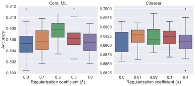
Figure 2: Influence of the regularization coefficient $\lambda$ on classification performance.

5.3.2 Accuracy with different fusion functions.

Figure 3 illustrates the results with different fusion operations (i.e. the $\text{COMBINE}_{3}$ function mentioned in Eq. (2)), including Sum, Max, Mean, and Concatenate operations. Sum and Mean achieve better results in proposed model because they require fewer parameters which can prevent the model from over-fitting and thus capture more information [33].

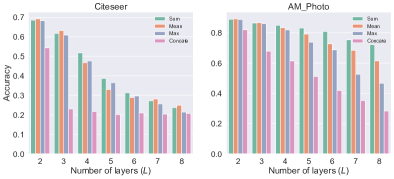
Figure 3: Influence of fusion functions on classification performance.

6 Conclusion

Most of the existing GNNs focus on undirected graphs, while the directed graphs are commonly encountered across different domains. The directional edge and asymmetric relationship are the most challenging aspects that make the directed GNNs difficult to train and implement in practice. We propose a simple yet effective method to model the asymmetric property of the directed graph within the GNN framework. The idea is to let each node play two asymmetric roles simultaneously: one is to act as an outgoing node, another is to act as an incoming node. The outgoing and incoming roles are quantified by two different embedding vectors. The outgoing embedding aims to capture the sending features of a node, and the incoming embedding aims to model the receiving features. With the two embeddings of each node, any directional edge in the graph can be interpreted by the outgoing embedding of its source node and the incoming embedding of its target node. Such one node but two roles setting can be easily applied to the current GNNs, by defining two aggregating/updating steps: one for aggregating/updating the receiving features of nodes, another for aggregating/updating the sending features of nodes. Experimental results on multiple real-world datasets illustrate that the proposed asymmetric GNN yields good performance in directed graph tasks.

References

- [1] Dominique Beaini, Saro Passaro, Vincent Létourneau, William L. Hamilton, Gabriele Corso, and Pietro Lió. Directional graph networks. In Proceedings of the Thirty-Eighth International Conference on Machine Learning, ICML 2021, volume 139, pages 748–758. PMLR, 2021.
- [2] Austin R Benson, David F Gleich, and Jure Leskovec. Higher-order organization of complex networks. Science, 353(6295):163–166, 2016.
- [3] Aleksandar Bojchevski and Stephan Günnemann. Deep gaussian embedding of graphs: Unsupervised inductive learning via ranking. In Proceedings of the Sixth International Conference on Learning Representations, ICLR 2018, pages 1–13, 2018.
- [4] Joan Bruna, Wojciech Zaremba, Arthur Szlam, and Yann LeCun. Spectral networks and deep locally connected networks on graphs. In Proceedings of the Second International Conference on Learning Representations, ICLR 2014, jan 2014.
- [5] Ming Chen, Zhewei Wei, Zengfeng Huang, Bolin Ding, and Yaliang Li. Simple and deep graph convolutional networks. In Proceedings of the Thirty-Seventh International Conference on Machine Learning, ICML 2020, pages 1725–1735. PMLR, 2020.
- [6] Michaël Defferrard, Xavier Bresson, and Pierre Vandergheynst. Convolutional neural networks on graphs with fast localized spectral filtering. In Proceedings of the Thirtieth International Conference on Neural Information Processing Systems, NeurIPS 2016, page 3844–3852, 2016.
- [7] Wenzheng Feng, Jie Zhang, Yuxiao Dong, Yu Han, Huanbo Luan, Qian Xu, Qiang Yang, Evgeny Kharlamov, and Jie Tang. Graph random neural networks for semi-supervised learning on graphs. In Proceedings of the Thirty-Fourth International Conference on Neural Information Processing Systems, NeurIPS 2020, volume 33, pages 22092–22103, 2020.
- [8] Bo Fu, Shilin Fu, Liyan Wang, Yuhan Dong, and Yonggong Ren. Deep residual split directed graph convolutional neural networks for action recognition. IEEE MultiMedia, 27(4):9–17, 2020.
- [9] Justin Gilmer, Samuel S. Schoenholz, Patrick F. Riley, Oriol Vinyals, and George E. Dahl. Neural message passing for quantum chemistry. In Proceedings of the Thirty-Fourth International Conference on Machine Learning, ICML 2017, volume 70, pages 1263–1272. PMLR, 2017.
- [10] Will Hamilton, Zhitao Ying, and Jure Leskovec. Inductive representation learning on large graphs. In Proceedings of the Thirty-First International Conference on Neural Information Processing Systems, NeurIPS 2017, volume 30, pages 1025–1035, 2017.
- [11] William L Hamilton. Graph representation learning. Synthesis Lectures on Artifical Intelligence and Machine Learning, 14(3):1–159, 2020.
- [12] Shlomo Hoory, Nathan Linial, and Avi Wigderson. Expander graphs and their applications. Bulletin of the American Mathematical Society, 43(4):439–561, 2006.
- [13] Thomas N. Kipf and Max Welling. Semi-supervised classification with graph convolutional networks. In Proceedings of the Fifth International Conference on Learning Representations, ICLR 2017, 2017.
- [14] Johannes Klicpera, Aleksandar Bojchevski, and Stephan Günnemann. Predict then propagate: Graph neural networks meet personalized pagerank. In Proceedings of the Seventh International Conference on Learning Representations, ICLR 2019, 2019.
- [15] Yujia Li, Daniel Tarlow, Marc Brockschmidt, and Richard S. Zemel. Gated graph sequence neural networks. In Proceedings of the Fourth International Conference on Learning Representations, ICLR 2016, 2016.
- [16] Yi Ma, Jianye Hao, Yaodong Yang, Han Li, Junqi Jin, and Guangyong Chen. Spectral-based graph convolutional network for directed graphs, 2019.
- [17] Federico Monti, Karl Otness, and Michael M. Bronstein. MOTIFNET: A motif-based graph convolutional network for directed graphs. In Proceedings of the 2018 IEEE Data Science Workshop, DSW 2018, pages 225–228. IEEE, 2018.
- [18] Aldo Pareja, Giacomo Domeniconi, Jie Chen, Tengfei Ma, Toyotaro Suzumura, Hiroki Kanezashi, Tim Kaler, Tao B. Schardl, and Charles E. Leiserson. Evolvegcn: Evolving graph convolutional networks for dynamic graphs. In Proceedings of the Thirty-Fourth AAAI Conference on Artificial Intelligence, AAAI 2020, volume 34, pages 5363–5370. AAAI Press, 2020.
- [19] Trang Pham, Truyen Tran, Dinh Q. Phung, and Svetha Venkatesh. Column networks for collective classification. In Proceedings of the Thirty-First AAAI Conference on Artificial Intelligence, AAAI 2017, pages 2485–2491. AAAI Press, 2017.
- [20] Karl Rohe, Tai Qin, and Bin Yu. Co-clustering directed graphs to discover asymmetries and directional communities. Proceedings of the National Academy of Sciences, 113(45):12679–12684, 2016.
- [21] Yu Rong, Wenbing Huang, Tingyang Xu, and Junzhou Huang. Dropedge: Towards deep graph convolutional networks on node classification. In Proceedings of the Eighth International Conference on Learning Representations, ICLR 2020, 2020.
- [22] Daniel Selsam, Matthew Lamm, Benedikt Bünz, Percy Liang, Leonardo de Moura, and David L. Dill. Learning a SAT solver from single-bit supervision. In Proceedings of the Seventh International Conference on Learning Representations, ICLR 2019, 2019.
- [23] Prithviraj Sen, Galileo Namata, Mustafa Bilgic, Lise Getoor, Brian Galligher, and Tina Eliassi-Rad. Collective classification in network data. AI magazine, 29(3):93–93, 2008.
- [24] Oleksandr Shchur, Maximilian Mumme, Aleksandar Bojchevski, and Stephan Günnemann. Pitfalls of graph neural network evaluation, 2018.
- [25] Lei Shi, Yifan Zhang, Jian Cheng, and Hanqing Lu. Skeleton-based action recognition with directed graph neural networks. In Proceedings of the IEEE Conference on Computer Vision and Pattern Recognition, 2019, pages 7912–7921. IEEE, 2019.
- [26] Christian Szegedy, Vincent Vanhoucke, Sergey Ioffe, Jonathon Shlens, and Zbigniew Wojna. Rethinking the inception architecture for computer vision. In Proceedings of the 2016 IEEE Conference on Computer Vision and Pattern Recognition, CVPR 2016, pages 2818–2826. IEEE Computer Society, 2016.
- [27] Veronika Thost and Jie Chen. Directed acyclic graph neural networks. In Proceedings of the Ninth International Conference on Learning Representations, ICLR 2021, 2021.
- [28] Zekun Tong, Yuxuan Liang, Changsheng Sun, Xinke Li, David S. Rosenblum, and Andrew Lim. Digraph inception convolutional networks. In Proceedings of the Thirty-fourth International Conference on Neural Information Processing Systems, NeurIPS 2020, volume 33, pages 17907–17918, 2020.
- [29] Zekun Tong, Yuxuan Liang, Changsheng Sun, David S. Rosenblum, and Andrew Lim. Directed graph convolutional network, 2020.
- [30] Petar Velickovic, Guillem Cucurull, Arantxa Casanova, Adriana Romero, Pietro Liò, and Yoshua Bengio. Graph attention networks. In Proceedings of the Sixth International Conference on Learning Representations, ICLR 2018, 2018.
- [31] Guangtao Wang, Rex Ying, Jing Huang, and Jure Leskovec. Multi-hop attention graph neural networks. In Proceedings of the Thirtieth International Joint Conference on Artificial Intelligence, IJCAI 2021, pages 3089–3096, 2021.
- [32] Felix Wu, Amauri H. Souza Jr., Tianyi Zhang, Christopher Fifty, Tao Yu, and Kilian Q. Weinberger. Simplifying graph convolutional networks. In Proceedings of the Thirty-Sixth International Conference on Machine Learning, ICML 2019, volume 97, pages 6861–6871. PMLR, 2019.
- [33] Keyulu Xu, Weihua Hu, Jure Leskovec, and Stefanie Jegelka. How powerful are graph neural networks? In Proceedings of the Seventh International Conference on Learning Representations, ICLR 2019, 2019.
- [34] Keyulu Xu, Chengtao Li, Yonglong Tian, Tomohiro Sonobe, Ken-ichi Kawarabayashi, and Stefanie Jegelka. Representation learning on graphs with jumping knowledge networks. In Proceedings of the Thirty-Fifth International Conference on Machine Learning, ICML 2018, volume 80, pages 5449–5458. PMLR, 2018.
- [35] Liang Yao, Chengsheng Mao, and Yuan Luo. Graph convolutional networks for text classification. In Proceedings of the Thirty-Third AAAI Conference on Artificial Intelligence, AAAI 2019, pages 7370–7377. AAAI Press, 2019.
- [36] Zhitao Ying, Jiaxuan You, Christopher Morris, Xiang Ren, William L. Hamilton, and Jure Leskovec. Hierarchical graph representation learning with differentiable pooling. In Proceedings of the Thirty-Second International Conference on Neural Information Processing Systems, NeurIPS 2018, volume 31, pages 4805–4815, 2018.
- [37] Muhan Zhang, Zhicheng Cui, Marion Neumann, and Yixin Chen. An end-to-end deep learning architecture for graph classification. In Proceedings of the Thirty-Second AAAI Conference on Artificial Intelligence, AAAI 2018, volume 32, pages 4438–4445. AAAI Press, 2018.
- [38] Muhan Zhang, Shali Jiang, Zhicheng Cui, Roman Garnett, and Yixin Chen. D-VAE: A variational autoencoder for directed acyclic graphs. In Proceedings of the Thirty-Third International Conference on Neural Information Processing Systems, NeurIPS 2019, pages 1586–1598, 2019.
- [39] Xitong Zhang, Nathan Brugnone, Michael Perlmutter, and Matthew J. Hirn. Magnet: A magnetic neural network for directed graphs, 2021.