Adaptive Differentially Private Empirical Risk Minimization

Abstract

We propose an adaptive (stochastic) gradient perturbation method for differentially private empirical risk minimization. At each iteration, the random noise added to the gradient is optimally adapted to the stepsize; we name this process adaptive differentially private (ADP) learning. Given the same privacy budget, we prove that the ADP method considerably improves the utility guarantee compared to the standard differentially private method in which vanilla random noise is added. Our method is particularly useful for gradient-based algorithms with time-varying learning rates, including variants of AdaGrad (Duchi et al., 2011). We provide extensive numerical experiments to demonstrate the effectiveness of the proposed adaptive differentially private algorithm.

1 Introduction

Publishing deep neural networks such as ResNets [He et al., 2016] and Transformers [Vaswani et al., 2017] (with billions of parameters) trained on private datasets has become a major concern in the machine learning community; these models can memorize the private training data and can thus leak personal information, such as social security numbers [Carlini et al., 2020]. Moreover, these models are vulnerable to privacy attacks, such as membership inference [Shokri et al., 2017, Gupta et al., 2021] and reconstruction [Fredrikson et al., 2015, Nakamura et al., 2020]. Therefore, over the past few years, a considerable number of methods have been proposed to address the privacy concerns described above. One main approach to preserving data privacy is to apply differentially private (DP) algorithms [Dwork et al., 2006a, 2014, Abadi et al., 2016, Jayaraman et al., 2020] to train these models on private datasets. Differentially private stochastic gradient descent (DP-SGD) is a common privacy-preserving algorithm used for training a model via gradient-based optimization; DP-SGD adds random noise to the gradients during the optimization process [Bassily et al., 2014, Song et al., 2013, Bassily et al., 2020].

To be concrete, consider the empirical risk minimization (ERM) on a dataset $\mathcal{D}=\{x_{i}\}_{i=1}^{n}$, where each data point $x_{i}\in{\cal X}$. We aim to obtain a private high dimensional parameter $\theta\in\mathcal{R}^{d}$ by solving

$$\min_{\theta\in\mathbb{R}^{d}}F(\theta):=\frac{1}{n}\sum_{i=1}^{n}f_{i}(\theta),\text{ with }f_{i}(\theta)=f(\theta;x_{i})$$ (1)

where the loss function $f(\cdot):\mathbb{R}^{d}\times\cal X\to\mathbb{R}$ is non-convex and smooth at each data point. To measure the performance of gradient-based algorithms for ERM, which enjoys privacy guarantees, we define the utility by using the expected $\ell_{2}$-norm of gradient, i.e., $\mathbb{E}[\|\nabla F(\theta)\|]$, where the expectation is taken over the randomness of the algorithm [Wang et al., 2017, Zhang et al., 2017, Wang et al., 2019, Zhou et al., 2020a]. The DP-SGD with a Gaussian mechanism solves ERM in (1) by performing the following update with the released gradient $g_{t}$ at the $t$-th iteration:

$$\text{DP-SGD: }\theta_{t+1}=\theta_{t}-\eta_{t}g_{t};g_{t}=\nabla f_{\xi_{t}}(\theta_{t})+Z,$$ (2)

where $Z\sim\mathcal{N}(0,\sigma^{2}I)$, $\xi_{t}\sim\text{Uniform}(\{1,2,\ldots,n\})$, and $\eta_{t}>0$ is the stepsize or learning rate. Choosing the appropriate stepsize $\eta_{t}$ is challenging in practice, as $\eta_{t}$ depends on the unknown Lipschitz parameter of the gradient $\nabla f(\theta;x_{i})$ Ghadimi and Lan [2013]. Recent popular techniques for tuning $\eta_{t}$ include adaptive gradient methods Duchi et al. [2011] and decaying stepsize schedules Goyal et al. [2017]. When applying non-constant stepsizes, most of the existing differentially private algorithms directly follow the standard DP-SGD strategy by adding a simple perturbation (i.e, $Z\sim\mathcal{N}(0,\sigma^{2}I)$) to each gradient over the entire sequence of iterations [Zhou et al., 2020a]. This results in a uniformly-distributed privacy budget for each iteration [Bassily et al., 2014].

Several theoretical, as well as experimental results, corroborate the validity of the DP-SGD method with a uniformly-distributed privacy budget [Bu et al., 2020, Zhou et al., 2020b, a]. Indeed, using a constant perturbation intuitively makes sense after noticing that the update in (2) is equivalent to $\theta_{t+1}=\theta_{t}-\eta_{t}\nabla f(\theta_{t};x_{\xi_{t}})-\eta_{t}Z$. This implies that the size of the true perturbation (i.e., $\eta_{t}Z$) added to the updated parameters is controlled by $\eta_{t}$. The decaying learning rate thus diminishes the true perturbation added to $\theta_{t}$. Although the DP-SGD method with decaying noise $\eta_{t}Z$ is reasonable, prior to this paper it was unknown whether this is the optimal strategy using the utility measure.

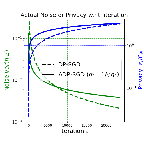
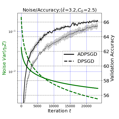
Figure 1: Comparison between $\alpha_{t}=1$ and $\alpha_{t}=1/\sqrt{\eta_{t}}$ in (3). Set the stepsize $\eta_{t}=1/\sqrt{20+t}$ and the same privacy budget at final iteration. The green curves in the left and right plots are the same; they correspond to the left vertical y-axis illustrating the actual Gaussian noise (i.e., $\eta_{t}\alpha_{t}Z$) added to the parameter $\theta_{t}$ for $\alpha_{t}=1$ (dash line) and $\alpha_{t}=1/\sqrt{\eta_{t}}$ (solid line). The blue (black) curves on the left (right) plot corresponding to the right vertical y-axis show the overall privacy (validation accuracy) for $\alpha_{t}=1$ (DP-SGD), represented by the dashed line, and $\alpha_{t}=1/\sqrt{\eta_{t}}$ (ADP-SGD), represented by the solid line. The variance of the perturbation using our proposed ADP-SGD decreases more slowly than that using DP-SGD, and so spreads across to entire optimization process more evenly than DP-SGD. Note that the privacy value $\bar{\varepsilon}=\varepsilon/16=3.2$ is based on the theoretical upper bound. The validation accuracy (black curves) is for CIFAR10 dataset with the gradient clipping $C_{G}=2.5$ comparable to $G$ (see detailed explanation in Section 6).

To study the above question, we propose adding a hyperparameter $\alpha_{t}>0$ to the private mechanism:

$$\text{{ADP-SGD}: }\theta_{t+1}=\theta_{t}-\eta_{t}g_{t};g_{t}=\nabla f_{\xi_{t}}(\theta_{t})+\eta_{t}\alpha_{t}Z.$$ (3)

The role of the hyperparameter $\alpha_{t}$ is to adjust the variance of the added random noise given the stepsize $\eta_{t}$. It is thus natural to add “adaptive” in front of the name DP-SGD and call our proposed algorithm ADP-SGD. To establish the privacy and utility guarantees of this new method, we first extend the advanced composition theorem [Dwork et al., 2014] so that it treats the case of a non-uniformly distributed privacy budget. We then show that our method achieves an improved utility guarantee when choosing $\alpha_{t}=1/\sqrt{\eta_{t}}$, compared to the standard method using uniformly-distributed privacy budget, which corresponds to $\alpha_{t}=1$.This relationship between $\alpha_{t}$ and $\eta_{t}$ is surprising. Given the same privacy budget and the decaying stepsize $\eta_{t}<1$, the best choice – $\alpha_{t}=1/\sqrt{\eta_{t}}$ – results in $\theta_{t+1}=\theta_{t}-\eta_{t}\nabla f(\theta_{t};x_{\xi_{t}})-\sqrt{\eta_{t}}Z$. This implies that the actual Gaussian noise $\sqrt{\eta_{t}}Z$ of ADP-SGD decreases more slowly than that of the conventional DP-SGD (i.e., $\eta_{t}Z$). To some extent, this is counter-intuitive in terms of convergence: one may anticipate that a more accurate gradient or smaller perturbation will be necessary as the parameter $\theta_{t}$ reaches a stationary point (i.e., as $\|\nabla F(\theta_{t})\|\to 0$) Lee and Kifer [2018]. See Figure 1 for an illustration. We will explain how this interesting finding is derived in Section 4.

Contribution.

Our contributions include:

• We propose an adaptive (stochastic) gradient perturbation method – “Adaptive Differentially Private Stochastic Gradient Descent” (ADP-SGD) (Algorithm 1 or (3)) – and show how it can be used to perform differentially private empirical risk minimization. We show that APD-SGD provides a solution to the core question of this paper: given the same overall privacy budget and iteration complexity, how should we select the gradient perturbation adaptively - across the entire SGD optimization process - to achieve better utility guarantees? To answer this, we establish the privacy guarantee of ADP-SGD (Theorem 4.1) and find that the best choice of $\alpha_{t}$ follows an interesting dynamic: $\alpha_{t}=1/\sqrt{\eta_{t}}$ (Theorem 4.2). Compared to the conventional DP-SGD, ADP-SGD with $\alpha_{t}=1/\sqrt{\eta_{t}}$ results in a better utility given the same privacy budget $\varepsilon$ and complexity $T$.

• As the ADP-SGD method can be applied using any generic $\eta_{t}$, we discuss the two widely-used stepsize schedules: (1) the polynomially decaying stepsize of the form $\eta_{t}=1/\sqrt{1+t}$, and (2) $\eta_{t}$ updated by the gradients Duchi et al. [2011]. When using $\eta_{t}=1/\sqrt{1+t}$, given the same privacy budgets $\varepsilon$, we obtain a stochastic sequence $\{\theta_{t}^{\rm ADP}\}$ for ADP-SGD with $\alpha_{t}=1/\sqrt{\eta_{t}}$, and $\{\theta_{t}^{\rm DP}\}$ for standard DP-SGD. We have the utility guarantees of the two methods, respectively

  $$\mathbb{E}[\|\nabla F(\theta_{\tau}^{\rm ADP})\|^{2}]=\widetilde{\mathcal{O}}\left(\frac{\log(T)}{\sqrt{T}}+\frac{d\sqrt{T}}{n^{2}\varepsilon^{2}}\right);\quad\quad\quad \mathbb{E}[\|\nabla F(\theta_{\tau}^{\rm DP})\|^{2}]=\widetilde{\mathcal{O}}\left(\frac{\log(T)}{\sqrt{T}}+\frac{d\log(T)\sqrt{T}}{n^{2}\varepsilon^{2}}\right)$$

  where $\tau:=\text{arg}\min_{k\in{[T-1]}}\mathbb{E}[\|\nabla F(\theta_{k})\|^{2}]$. Compared to the standard DP-SGD, ADP-SGD with $\alpha_{t}=1/\sqrt{\eta_{t}}$ improves the bound by a factor of $\mathcal{O}(\log(T))$ when $T$ and $d$ are large (i.e. high-dimensional settings). When $\eta_{t}$ is updated by the gradients Duchi et al. [2011], the same result holds. See Section 5 for the detailed discussion.

• Finally, we perform numerical experiments to systematically compare the two algorithms: ADP-SGD ($\alpha_{t}=1/\sqrt{\eta_{t}}$) and DP-SGD. In particular, we verify that ADP-SGD with $\alpha_{t}=1/\sqrt{\eta_{t}}$ consistently outperforms DP-SGD when $d$ and $T$ are large. Based on these theoretical bounds and supporting numerical evidence, we believe ADP-SGD has important advantages over past work on differentially private empirical risk minimization.

Notation.

In the paper, $[N]:=\{0,1,2,\dots,N\}$ and $\{\cdot\}:=\{\cdot\}_{t=1}^{T}$. We write $\|\cdot\|$ for the $\ell_{2}$-norm. $F^{*}$ is a global minimum of $F$ assuming $F^{*}>0$. We use $D_{F}:=F(\theta_{0})-F^{*}$ and set stepsize $\eta_{t}=\eta/b_{t+1}$.

2 Preliminaries

We first make the following assumptions for the objective loss function in (1).

Assumption 2.1.

Each component function $f(\cdot)$ in (1) has $L$-Lipschitz gradient, i.e.,

$$\|\nabla f(x)-\nabla f(y)\|\leq L\|x-y\|,\quad\forall x,y\in\mathbb{R}^{d}.$$ (4)

Assumption 2.2.

Each component function $f(\cdot)$ in (1) has bounded gradient, i.e.,

$$\|\nabla f(x)\|\leq G,\quad\forall x\in\mathbb{R}^{d}.$$ (5)

The bounded gradient assumption is a common assumption for the analysis of DP-SGD algorithms [Wang et al., 2017, Zhou et al., 2020a, b] and also frequently used in general adaptive gradient methods such as Adam [Reddi et al., 2021, Chen et al., 2018, Reddi et al., 2018]. One recent popular approach to relax this assumption is using the gradient clipping method [Chen et al., 2020, Andrew et al., 2019, Pichapati et al., 2019], which we will discuss more in Section 6 as well as in Appendix A. Nonetheless, this assumption would serve as a good starting point to analyze our proposed method. Next, we introduce differential privacy [Dwork et al., 2006b].

Definition 2.1 ($(\varepsilon,\delta)$-DP).

A randomized mechanism $\mathcal{M}:\mathcal{D}\rightarrow\mathcal{R}$ with domain $\mathcal{D}$ and range $\mathcal{R}$ is $(\varepsilon,\delta)$-differentially private if for any two adjacent datasets $\mathcal{D},\mathcal{D}^{\prime}$ differing in one sample, and for any subset of outputs $S\subseteq\mathcal{R}$, we have

$$\text{Pr}[\mathcal{M}(D)\in S]\leq e^{\varepsilon}\text{Pr}[\mathcal{M}(D^{\prime})\in S]+\delta.$$

Lemma 2.1 (Gaussian Mechanism).

For a given function $h:\mathcal{D}\to\mathbb{R}^{d}$, the Gaussian mechanism $\mathcal{M}(\mathcal{D})=h(\mathcal{D})+Z$ with $Z\sim\mathcal{N}(0,\sigma^{2}I_{d})$ satisfies $(\sqrt{2\log(1.25/\delta)}\Delta/\sigma,\delta)$-DP, where $\Delta=\sup_{\mathcal{D},\mathcal{D}^{\prime}}\|h(\mathcal{D})-h(\mathcal{D}^{\prime})\|$, $\mathcal{D},\mathcal{D}^{\prime}$ are two adjacent datasets, and $\varepsilon,\delta>0$.

To achieve differential privacy, we can use the above Gaussian mechanism [Dwork et al., 2014]. In our paper, we consider iterative differentially private algorithms, which prompts us to use privacy composition results to establish the algorithms’ privacy guarantees after the completion of the final iteration. To this end, we extend the advanced composition theorem [Dwork et al., 2014] to the case in which each mechanism $\mathcal{M}_{i}$ has its own specific $\varepsilon_{i}$ and $\delta_{i}$ parameters.

Lemma 2.2 (Extended Advanced Composition).

Consider two sequences $\{\varepsilon_{i}\}_{i=1}^{k},\{\delta_{i}\}_{i=1}^{k}$ of positive numbers satisfying $\varepsilon_{i}\in(0,1)$ and $\delta_{i}\in(0,1)$. Let $\mathcal{M}_{i}$ be $(\varepsilon_{i},\delta_{i})$-differentially private for all $i\in\{1,2,\ldots,k\}$. Then $\mathcal{M}=(\mathcal{M}_{1},\ldots,\mathcal{M}_{k})$ is $(\tilde{\varepsilon},\tilde{\delta})$-differentially private for $\delta^{\prime}\in(0,1)$ and

$$\tilde{\varepsilon} =\sqrt{\sum_{i=1}^{k}2\varepsilon_{i}^{2}\log\left(\frac{1}{\delta^{\prime}}\right)}+\sum_{i=1}^{k}\frac{\varepsilon_{i}(e^{\varepsilon_{i}}-1)}{(e^{\varepsilon_{i}}+1)},\quad\tilde{\delta}=1-(1-\delta_{1})(1-\delta_{2})\ldots(1-\delta_{k})+\delta^{\prime}.$$

When $\varepsilon_{i}=\varepsilon_{0}$ and $\delta_{i}=\delta_{0}$ for all $i$, Lemma 2.2 reduces to the classical advanced composition theorem [Dwork et al., 2014] restated in Lemma A.2 in the Appendix.

3 The ADP-SGD algorithm

In this section, we present our proposed algorithm: adaptive differentially private stochastic gradient descent (ADP-SGD, Algorithm 1). The “adaptive” part of the algorithm is tightly connected with the choice of the hyper-parameter $\alpha_{t}$ (see line 5 of Algorithm 1). For $\alpha_{t}=1$, ADP-SGD reduces to DP-SGD. As mentioned before, we aim to investigate whether an uneven allocation of the privacy budget for each iteration (via ADP-SGD) will provide a better utility guarantee than the default DP-SGD given the same privacy budget. To achieve this, our proposed ADP-SGD with hyper-parameter $\alpha_{t}$ adjusts the privacy budget consumed at the $t$-th iteration according to the current learning rate $\eta/b_{t+1}$ (see line 6 of Algorithm 1). Moreover, we will update $\alpha_{t}$ dynamically (see line 5 of Algorithm 1) and show how to choose $\alpha_{t}$ in Section 4. Before proceeding to analyze Algorithm 1, we state Definition 3.1 to clearly explain the adaptive privacy mechanism for the algorithm.

Definition 3.1 (Adaptive Gaussian Mechanism).

At iteration $t$ in Algorithm 1, the privacy mechanism $\mathcal{M}_{t}:$ $\mathbb{R}^{d}\to\mathbb{R}^{d}$ is:

$$\mathcal{M}_{t}(X)=\nabla f(\theta_{t};x_{\xi_{t}})+\alpha_{t+1}c_{t}.$$

The hyper-parameter $\alpha_{t+1}$ is adaptive to the DP-SGD algorithm specifically to the stepsize $\eta_{t}:=\eta/b_{t}$.

Algorithm 1 ADP-SGD (DP-SGD if $\alpha_{t}=1$)

1:Input: $\theta_{0},b_{0},\alpha_{0}$ and $\eta>0$

2:for $t=0,1,\ldots,T-1$ do

3:     $\xi_{t}\sim\text{Uniform}(1,...,n)$ and $c_{t}\sim\mathcal{N}(0,\sigma^{2}I)$

4:     update $b_{t+1}=\phi_{1}(b_{t},\nabla f(\theta_{t};x_{\xi_{t}}))$

5:     update $\alpha_{t+1}=\phi_{2}(\alpha_{t},b_{t+1})$

6:     release $g^{b}_{t}=\frac{\eta}{b_{t+1}}(\nabla f(\theta_{t};x_{\xi_{t}})+\alpha_{t+1}c_{t})$

7:     update $\theta_{t+1}=\theta_{t}-g^{b}_{t}$

8:end for

Algorithm 1 is a general framework that can cover many variants of stepsize update schedules, including the adaptive gradient algorithms [Duchi et al., 2011, Kingma and Ba, 2014]. Rewriting $\eta_{t}=\eta/b_{t+1}$ in Algorithm 1 is equivalent to (3). In particular, we use functions $\phi_{1}:\mathbb{R}^{2}\to\mathbb{R}$ and $\phi_{2}:\mathbb{R}^{2}\to\mathbb{R}$ to denote the updating rules for parameters $b_{t}$ and $\alpha_{t}$, respectively. For example, when $\phi_{1}$ is $1/\sqrt{a+ct}$, $\phi_{2}$ is the constant $1$ for all $t$ and $a,c>0$, ADP-SGD reduces to DP-SGD with polynomial decaying stepsizes [Bassily et al., 2014]. When $\phi_{1}$ is $b_{t+1}=\sqrt{b_{t}^{2}+\|\nabla f(\theta_{t};x_{\xi_{t}})\|^{2}}$ and $\phi_{2}$ is the constant 1, the algorithm reduces to DP-SGD with a variant of adaptive stepsizes [Duchi et al., 2011]. In particular, if we choose $\phi_{2}$ to be 0, the algorithm reduces to the vanilla SGD.

Similar to classical works on the convergence of the SGD algorithm [Bassily et al., 2020, Bottou et al., 2018, Ward et al., 2019], we will use Assumption 3.1 in addition to Assumption 2.2 and Assumption 2.1.

Assumption 3.1.

$\nabla f(\theta_{t};x_{\xi_{t}})$ is an unbiased estimator of $\nabla F(\theta_{k})$. The random indices $\xi_{t}$, $t=0,1,2,\dots,$ are independent of each other and also independent of $\theta_{t}$ and $c_{1},\ldots,c_{t-1}$.

Having defined the ADP-SGD algorithm and established our assumptions, in what follows, we will be answering the paper’s central question: Given the same privacy budget $\varepsilon$, how should one design the gradient perturbation parameters $\alpha_{t}$ adaptively for each iteration $t$ to achieve a better utility guarantee? Solving this question is of paramount importance as one can only run these algorithms for a finite number of iterations. Therefore, given these constraints, a clear and efficient strategy for improving the constants of the utility bound is necessary.

4 Theoretical results for ADP-SGD

In this section, we provide the main results for our method – the privacy and utility guarantees.

Theorem 4.1 (Privacy Guarantee).

Suppose the sequence $\{\alpha_{t}\}_{t=1}^{T}$ is known in advance and that Assumption 2.2 holds. Algorithm 1 satisfies $(\varepsilon,\delta)$-DP if the random noise $c_{t}$ has variance

$$\sigma^{2} =\frac{(16G)^{2}B_{\delta}}{n^{2}\varepsilon^{2}}\;{\sum_{t=0}^{T-1}\frac{1}{\alpha^{2}_{t+1}}}\text{ with }B_{\delta}=\log\left(\frac{16T}{n\delta}\right)\log\left(\frac{1.25}{\delta}\right).\vspace{-0.6cm}$$ (6)

The theorem is proved by using Lemma 2.2 and Definition 3.1 (see Section C.1 for details). Note that the term $B_{\delta}$ could be improved by using the moments accountant method [Mironov et al., 2019], to $\mathcal{O}(\log(1.25/\delta))$ independent of $T$ but with some additional constraints [Abadi et al., 2016]. We keep this format of $B_{\delta}$ as in (6) in order to compare directly with [Bassily et al., 2014].

Theorem 4.1 shows that $\sigma^{2}$ must scale with $\sum_{t=1}^{T}1/\alpha^{2}_{t}$. When the complexity $T$ increases, the variance $\sigma^{2}$, regarded as a function of $T$, could be either large or small, depending on the sequence $\{\alpha_{t}\}$.

$$\vspace{-0.15cm}\text{If }\alpha_{t}^{2}\propto t^{p},p\in[0,1],\quad\text{then }\textstyle\sigma^{2}\propto\begin{cases}T^{1-p}&0\leq p<1\\ \log(T)&p=1\end{cases}$$

and $p=0$ is the default DP-SGD. From a convergence view, $\theta_{t+1}=\theta_{t}-\eta_{t}\nabla f(\theta_{t};x_{\xi_{t}})-\eta_{t}\alpha_{t}Z$ implies that the actual Gaussian noise added to the updated parameter $\theta_{t}$ has variance $\eta_{t}^{2}\alpha_{t}^{2}\sigma^{2}$. Therefore, it is subtle to determine what $p$ would be the best choice for ensuring convergence. In Theorem 4.2, we will see that the optimal choice of the sequence $\{\alpha_{t}\}_{t=1}^{T}$ is closely related to the stepsize.

Theorem 4.2 (Convergence for ADP-SGD).

Suppose we choose $\sigma^{2}$ - the variance of the random noise in Algorithm 1 - according to (6) in Theorem 4.1 and that Assumption 2.1, 2.2 and 3.1 hold. Furthermore, suppose $\alpha_{t},b_{t}$ are deterministic. The utility guarantee of Algorithm 1 with $\tau\triangleq\text{arg}\min_{k\in{[T-1]}}\mathbb{E}[\|\nabla F(\theta_{k})\|^{2}]$ and $B_{\delta}=\log(16T/(n\delta))\log(1.25/\delta)$ is

$$\mathbb{E}\|\nabla F(\theta_{\tau})\|^{2}\leq\frac{1}{\sum_{t=0}^{T-1}b_{t+1}}\left(W_{opt}+\frac{d(16G)^{2}B_{\delta}}{2n^{2}\varepsilon^{2}}M(\{\alpha_{t}\},\{b_{t}\})\right)$$ (7)

where $W_{opt}:=\frac{D_{F}}{\eta}+\frac{\eta L}{2}\sum_{t=0}^{T-1}\frac{\mathbb{E}\left[\|\nabla f(\theta_{t},{\xi_{t}})\|^{2}\right]}{b^{2}_{t+1}}$ and $M(\{\alpha_{t}\},\{b_{t}\}){\triangleq}\textstyle\sum_{t=1}^{T}(\alpha_{t}/b_{t})^{2}\sum_{t=1}^{T}1/\alpha^{2}_{t}.$

Although the theorem assumes independence between $b_{t+1}$ and the stochastic gradient $\nabla f(\theta_{t};x_{\xi_{t}})$, we shall see in Section 5.2 that a similar bound holds for correlated $b_{t}$ and $\nabla f(\theta_{t};x_{\xi_{t}})$.

Remark 4.1 (An optimal relationship between $\alpha_{t}$ and $b_{t}$).

According to (7), the utility guarantee of Algorithm 1 consists of two terms. The first term ($W_{opt}$) corresponds to the optimization error and the last term ($\frac{d(16G)^{2}B_{\delta}}{2n^{2}\varepsilon^{2}}M(\{\alpha_{t}\},\{b_{t}\})$) is introduced by the privacy mechanism, which is also the dominating term. Note that if we fix $\{b_{t}\}$ and minimize $M$ with respect to $\{\alpha_{t}\}$, the minimal value denoted by $M_{\rm adp}$ expresses as

$$\vspace{-0.2cm}\min_{\{\alpha_{t}\}}M(\{\alpha_{t}\},\{b_{t}\})=M_{\rm adp}\triangleq\big{(}\textstyle\sum_{t=0}^{T-1}1/b_{t+1}\big{)}^{2}.\vspace{-0.2cm}$$ (8)

Furthermore, $M(\{\alpha_{t}\},\{b_{t}\})=M_{\rm adp}$ if $\alpha^{2}_{t}=b_{t}.$ Therefore, if we choose $\alpha_{t},b_{t}$ such that the relationship of $\alpha^{2}_{t}=b_{t}$ holds, we can achieve the minimum utility guarantee for Algorithm 1.

Based on the utility bound in Theorem 4.2, we now compare the strategies between using the arbitrary setting of $\{\alpha_{t}\}$ and the optimal setting $\alpha^{2}_{t}=b_{t}$ by examining the ratio $M(\{\alpha_{t}\},\{b_{t}\})/M_{\rm adp}$; a large value of this ratio implies a significant reduction in the utility bound is achieved by using Algorithm 1 with $\alpha_{t}=\sqrt{b_{t}}$. For example, for the standard DP-SGD method, the function $M$ reduces to $M_{\rm dp}\triangleq T\sum_{t=0}^{T-1}{1}/{b^{2}_{t+1}}$. Our proposed method - involving $\alpha_{t}=\sqrt{b_{t}}$ - admits a bound improved by a factor of

$${M_{\rm dp}}/{M_{\rm adp}}=T\left({\textstyle\sum_{t=0}^{T-1}{1}/{b^{2}_{t+1}}}\right)/\left({\textstyle\sum_{t=0}^{T-1}{1}/{b_{t+1}}}\right)^{2}\overset{(a)}{\geq}1,$$

where (a) is due to the Cauchy-Schwarz inequality; thus, ADP-SGD is not worse than DP-SGD for any choice of $\{b_{t}\}$. In the following section, we will analyze this factor of $M_{\rm dp}/M_{\rm adp}$ for two widely-used stepsize schedules: (a) the polynomially decaying stepsize given by $\eta_{t}=1/\sqrt{1+t}$; and (b) a variant of adaptive gradient methods [Duchi et al., 2011].

Note that, in addition to $\alpha^{2}_{t}=b_{t}$, there are other relationships between the sequences $\{(\alpha_{t}/b_{t})^{2}\}$ and $\{\alpha^{2}_{t}\}$ that could lead to the same $M_{\rm adp}$. For instance, setting $\alpha_{t}\alpha_{T-(t-1)}=b_{t}$ is another possibility. Nevertheless, in this paper, we will focus on the $\alpha_{t}^{2}=b_{t}$ relation, and leave the investigation of other appropriate choices to future work. We emphasize that the bound in Theorem 4.2 only assumes $f$ to have Lipschitz smooth gradients and be bounded. Thus, the theorem applies to both convex or non-convex functions. Since our focus is on the improvement factor $M_{\rm dp}/M_{\rm tadp}$, we will assume our functions are non-convex, but the results will also hold for convex functions.

5 Examples for ADP-SGD

We now analyze the convergence bound given in Theorem 4.2 and obtain an explicit form for $M$ in terms of $T$ by setting the stepsize to be $1/b_{t+1}\propto 1/\sqrt{t}$, which is closely related to the polynomially decreasing rate of adaptive gradient methods [Duchi et al., 2011, Ward et al., 2019] studied in Section 5.2.

Constant stepsize v.s. time-varying stepsize.

If the constant step size is used, then there is no need to use the adaptive DP mechanism proposed in this paper as we verify that constant perturbation to the gradient is optimal in terms of convergence. However, as we explained in the introduction, to ease the difficulty of stepsize tuning, time-varying stepsize is widely used in many practical applications of deep learning. We will discuss two examples below. In these cases, the standard DP mechanism (i.e., constant perturbation to the gradient) is not the most suitable technique, and our proposed adaptive DP mechanism can give better utility results.

Achieving $\log T$ improvement.

We present Proposition 5.1 and Proposition 5.2 to show that our method achieves $\log(T)$ improvement over the vanilla DP-SGD. Although this $\log(T)$ improvement can also be achieved by using the moments accountant method (MAM) [Mironov et al., 2019], we emphasize that our proposed method is orthogonal and complementary to MAM. This is because the $\log(T)$ improvement using MAM is over $B_{\delta}$ (see discussion after Theorem 4.1), while ours is during the optimization process depending on stepsizes. Nevertheless, since the two techniques are complementary to each other, we can apply them simultaneously and achieve a $\log^{2}(T)$ improvement over DP-SGD using the advanced composition for $O(1/\sqrt{t})$ stepsizes, compared to a $\log(T)$ improvement using either of them. Thus, an adaptive DP mechanism for algorithms with time-varying stepsizes is advantageous.

5.1 Example 1: ADP-SGD with polynomially decaying stepsizes

The first case we consider is the stochastic gradient descent with polynomially decaying stepsizes. More specifically, we let $b_{t}=(a+ct)^{1/2}$, $a>0,c>0$.

Proposition 5.1 (ADP-SGD v.s. DP-SGD for a polynomially decaying stepsize schedule).

Under the conditions of Theorem 4.2 on $f$ and $\sigma^{2}$, let $b_{t}=(a+ct)^{1/2}$ with $a>0,c>0$ in Algorithm 1. Denote $\tau=\arg\min_{t\in[T-1]}\mathbb{E}[\|\nabla F(\theta_{t})\|^{2}]$, and $B_{\delta}=\log(16T/(n\delta))\log(1.25/\delta)$. If we choose $T\geq 5+4{a}/{c}$, we have the following utility guarantee for ADP-SGD ($\alpha_{t}^{2}=b_{t}$) and DP-SGD ($\alpha_{t}^{2}=1$) respectively,

$$\textbf{(ADP-SGD) }\quad\mathbb{E}[\|\nabla F(\theta_{\tau}^{\rm ADP})\|^{2}]\leq\frac{W^{decay}_{opt}}{\sqrt{T-1}}+\frac{\eta dL(16G)^{2}B_{\delta}\sqrt{T}}{2n^{2}\varepsilon^{2}\sqrt{c}};$$ (9)

$$\textbf{(DP-SGD) }\quad\mathbb{E}[\|\nabla F(\theta_{\tau}^{\rm DP})\|^{2}]\leq\frac{W^{decay}_{opt}}{\sqrt{T-1}}+\frac{\eta dL(16G)^{2}B_{\delta}\sqrt{T}\log\left(1+T\frac{c}{a}\right)}{n^{2}\varepsilon^{2}\sqrt{c}}.$$ (10)

where $W^{decay}_{opt}=\sqrt{c}\left(\frac{D_{F}}{\eta}+\frac{\eta G^{2}LB_{T}}{2c}\right)$.

The proof of Proposition 5.1 is given in Section D.1 and Section D.2. Proposition 5.1 implies $M_{\rm dp}/M_{\rm adp}={\cal O}(\log T)$ – that is, ADP-SGD has an improved utility guarantee compared to DP-SGD. Such an improvement can be significant when $d$ is large and $LG^{2}$ is large.

5.2 Example 2: ADP-SGD with adaptive stepsizes

We now examine another choice of the term $b_{t}$, which relies on a variant of adaptive gradient methods [Duchi et al., 2011]. To be precise, we assume $b_{t}$ is updated according to the norm of the gradient, i.e., $b_{t+1}^{2}=b_{t}^{2}+\max\{\|\nabla f(\theta_{t};x_{\xi_{t}})\|^{2},\nu\}$, where $\nu>0$ is a small value to prevent the extreme case in which $1/b_{t+1}$ goes to infinity (when $b_{0}^{2}=\|\nabla f(\theta_{t};x_{\xi_{t}})\|^{2}\to 0$, then $\eta/b_{1}\to\infty$). We choose this precise equation formula because it is simple, and it also represents the core of adaptive gradient methods - updating the stepsize on-the-fly by the gradients [Levy et al., 2018, Ward et al., 2019]. The conclusions for this variant may transfer to other versions of adaptive stepsizes, and we defer this to future work.

Observe that $b_{t}\propto t^{1/2}$ since $b_{t}^{2}\in[b_{0}^{2}+tv,b_{0}^{2}+tG]$, which at a first glance indicates that the bound for this adaptive stepsize could be derived via a straightforward application of Proposition 5.1. However, since $b_{t}$ is now a random variable correlated to the stochastic gradient $\nabla f(\theta_{t};x_{\xi_{t}})$, we cannot directly apply Theorem 4.2 to study $b_{t}$. To tackle this, we adapt the proof technique from [Ward et al., 2019] and obtain Theorem D.1, which we defer to Appendix D.3.

As we see, $b_{t}$ is updated on the fly during the optimization process. Applying our propsoed method with $\alpha_{t}^{2}=b_{t}$ for this adaptive stepsize is not possible since $\alpha_{t}$ has to be set beforehand according to Equation (6) in Theorem 4.1. To address this, we note $b_{t}^{2}\in[b_{0}^{2}+tv,b_{0}^{2}+tG]$. Thus, we propose to set $\alpha_{t}^{2}=\sqrt{b_{0}^{2}+tC}$ for some $C\in[\nu,G^{2}]$ and obtain Proposition 5.2 based on Theorem D.1.

Proposition 5.2 (ADP v.s. DP with an adaptive stepsize schedule).

Under the same conditions of Theorem D.1 on $f$, $\sigma^{2}$, and $b_{t}$, if $\alpha_{t}=(b_{0}^{2}+tC)^{1/4}$ for some $C\in[\nu,G^{2}]$, then

$$\textbf{(ADP-SGD)}\quad\mathbb{E}\|\nabla F(\theta_{\tau}^{\rm ADP})\|^{2}\leq\frac{W_{opt}^{adap}}{\sqrt{T-1}}+\frac{128G^{3}\eta dLB_{\delta}\sqrt{T}}{n^{2}\varepsilon^{2}\nu}.$$

$$\textbf{(DP-SGD)}\quad\mathbb{E}\|\nabla F(\theta_{\tau}^{\rm DP})\|^{2}\leq\frac{W_{opt}^{adap}}{\sqrt{T-1}}+\frac{32G^{3}\eta dLB_{\delta}\sqrt{T}\log\left(1+T\frac{\nu}{b_{0}^{2}}\right)}{n^{2}\varepsilon^{2}\nu}.$$

where $\textstyle W_{opt}^{adap}=2G\left(2G+\frac{\eta L}{2}\right)\left(1+\log\left(\frac{T(G^{2}+\nu^{2})}{b_{0}^{2}}+1\right)\right)+\frac{2GD_{F}}{\eta}$.

See the proof in Section D.4. Similar to the comparison in Proposition 5.1, the key difference between two bounds in Proposition 5.2 is the last term; using ADP-SGD gives us a tighter utility guarantee than the one provided by DP-SGD by a factor of $\mathcal{O}(\log(T))$. This improvement is significant when the dimension $d$ is very high, or when either $L$, $G$, or $T$ are sufficiently large. Note that the bound in Proposition 5.2 does not reflect the effect of the different choice of $C$, as the bound corresponds to the worst case scenarios. We will perform experiments testing a wide range of $C$ values and this will allow us to thoroughly examine the properties of ADP-SGD for adaptive stepsizes.

6 Experiments

In this section, we present numerical results to support the theoretical findings of our proposed methods. We perform two sets of experiments: (1) when $\eta_{t}$ is polynomially decaying, we compare ADP-SGD ($\alpha_{t}^{2}=b_{t}$) with DP-SGD (setting $\alpha_{t}=1$ in Algorithm 1 ); and (2) when $b_{t}$ is updated by the norm of the gradients, we compare ADP-SGD ($\alpha_{t}^{2}=\sqrt{b_{0}^{2}+tC}$) with DP-SGD. The first set of experiments is designed to examine the case when the learning rate is precisely set in advanced (i.e., Proposition 5.1), while the second concerns when the learning rate is not known ahead (i.e., Proposition 5.2). In addition to the experiments above, in the supplementary material (Section F.3), we present strong empirical evidence in support of the claim that using a decaying stepsize schedule yields better results than simply employing a constant stepsize schedule. See Section G for our code demonstration.

Assumption 2.2 and the gradient clipping method.

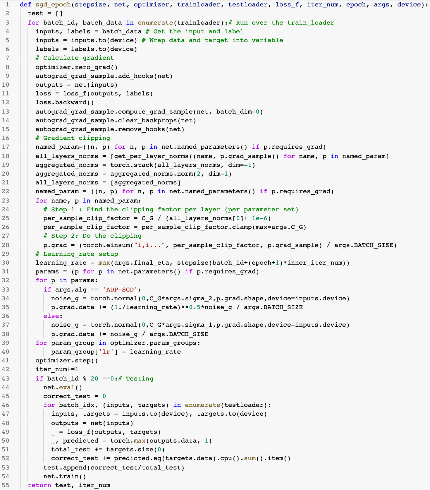
Figure 8: Sample code (one epoch) based on PyTorch for training a CNN model over CIFAR10 data, whose results are shown in Table 5 and 4

One limitation for the above proposition is the bounded gradient (Assumption 2.2). However, as discussed in Section 2, this is common. But $G$ could be very large, particularly for all $\theta\in\mathbb{R}^{d}$ in highly over-parameterized models (such as neural networks). To make the algorithm work in practice, we use gradient clipping [Chen et al., 2020, Andrew et al., 2019, Pichapati et al., 2019]. That is, given the current gradient $\nabla f_{\xi_{t}}(\theta_{t})$, we apply a function $h(\cdot;C_{G}):\mathbb{R}^{d}\to\mathbb{R}^{d}$, which depends on the the positive constant $C_{G}>0$ such that of $\|h(\nabla f_{\xi_{t}}(\theta_{t})\|\leq C_{G}$. Thus, the implementation of our algorithms (sample codes are shown in Figure 8) are

ADP-SGD: $$\theta_{t+1}=\theta_{t}-\eta_{t}g_{t};\quad g_{t}=h(\nabla f_{\xi_{t}}(\theta_{t}),C_{G})+\eta_{t}\alpha_{t}Z.$$ (11)

DP-SGD: $$\theta_{t+1}=\theta_{t}-\eta_{t}g_{t};\quad g_{t}=h(\nabla f_{\xi_{t}}(\theta_{t}),C_{G})+Z,$$ (12)

Regarding the convergence result of using the gradient clipping method instead of the bounded gradient assumption (Assumption 2.2), [Chen et al., 2020] show that if the gradient distribution is “approximately” symmetric, then the gradient norm goes to zero (Corollary 1). Furthermore, [Chen et al., 2020] showed (in Theorem 5) that the convergence of DP-SGD with clipping (without bounded gradient assumption) is $O(\sqrt{d}/(n\varepsilon))+$ clipping bias with the specified constant learning rate $O(1/\sqrt{T})$.

There is a straightforward way to apply our adaptive perturbation to the above clipping result (e.g., Theorem 5 in [Chen et al., 2020]) using the time-varying learning rate. The bounds for ADP-SGD and DP-SGD respectively are (9)+clipping bias and (10)+clipping bias where the constant $G$ in (9) and (10) is now replaced with $C_{G}$. Thus, there is still a $log(T)$ factor gain if clipping bias is not larger than the bounds in (9) and (10). In our experiments, we will be using various gradient clipping values $C_{G}\in\{0.5,1.0,2.5,5.0\}$ to understand how it affects our utility.

Datasets and models.

We perform our experiments on CIFAR-10 [Krizhevsky et al., 2009], using a convolution neural network (CNN). See our CNN design in the appendix. Notably, following previous work [Abadi et al., 2016], the CNN model is pre-trained on CIFAR-100 and fined-tuned on CIFAR-10. The mini-batch size is $256$, and each independent experiment runs on one GPU. We set $\eta=1$ in Algorithm 1 (line 6) and use the gradient clipping with $C_{G}\in\{0.5,1,2.5,5\}$ [Chen et al., 2020, Andrew et al., 2019, Pichapati et al., 2019]. Note that one might need to think about $C_{G}$ as being approximately closer to the bounded gradient parameter $G$. We provide a more detailed discussion in Appendix 6.1. The privacy budget is set to be $\bar{\varepsilon}=\varepsilon/C_{\varepsilon}\in\{0.8,1.2,1.6,3.2,6.4\}$ and we choose $\delta=10^{-5}$. Given these privacy budgets, we calculate the corresponding variance by Theorem 4.1 (See Appendix G for the code to obtain $\sigma$). We acknowledge that our empirical investigation is limited by the computing budget and this limitation forced us to choose between diversity in the choice of iteration complexity $T$ and type of stepsizes as opposed to diversity in the model architectures and datasets.

Performance measurement.

There are $50000$ images used for training and $10000$ images for validation, respectively. We repeat the experiments five times. For the $i$-th independent experiment, we calculate the validation accuracy at every 20 iterations and select the best validation accuracy $acc^{best}_{i}$ during the optimization process (over the entire iteration $\{t\}_{t=1}^{T}$). In Table 1 and Table 2, we report the average and standard deviation of $\{\text{acc}^{best}_{i}\}_{i=1}^{5}$, which is closely related to $\min_{t\in[T]}\mathbb{E}\|\nabla F(\theta_{t}^{\rm ADP})\|^{2}$ and $\min_{t\in[T]}\mathbb{E}\|\nabla F(\theta_{t}^{\rm DP})\|^{2}$, the convergence metric for our theoretical analysis in Theorem 4.2. Additionally, to further understand the method’s final performance, we report in Table 4 and 5 the average and standard deviation of the accuracy $\{\text{acc}^{last}_{i}\}_{i=1}^{5}$ where $\text{acc}^{last}_{i}$ represents the validation accuracy at iteration $T$ for the $i$-th experiment.

6.1 ADP-SGD v.s. DP-SGD for polynomially decaying stepsizes

We focus on understanding the optimality of the theoretical guarantees of Theorem 4.2 and Proposition 5.1; the experiments help us further understand how this optimality reflects in generalization. We consider training with $T=11760,23520,39200$ iterations corresponding to $60,120,200$ training epochs (196 iterations/epoch), which represents the practical scenarios of limited, standard and large computational time budgets. We use two kinds of monotone learning rate schedules: i) $\eta_{t}=0.1-\alpha_{T}\sqrt{t}$ (see orange curves in Figure 2) and report the results in Table 1; ii) $\eta_{t}=\eta/b_{t+1}=1/\sqrt{20+t}$ (see blue curves in Figure 2), in which the results are given in Table 2. The former learning rate schedule is designed to make sure the learning rate reaches close to zero at $T$, while the latter one is to match precisely Proposition 5.1.

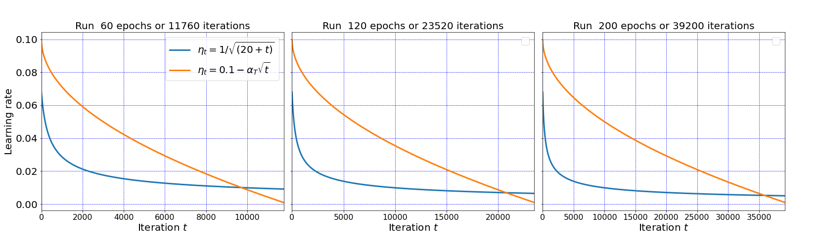
Figure 2: Two schedules of decaying learning rates. The blue curve in three plots are the same, while the orange ones are different. The blue learning rate is $\eta_{t}=\eta/b_{t+1}=1/\sqrt{20+t}$ used for Table 2 and 5. The orange ones, used for Table 1 and 4, are described by $\eta_{t}=0.1-\alpha_{T}\sqrt{t}$ where $\alpha_{T}$ is the ratio depending on the final iterations $T$ (i.e. $196\times$epochs) such that the learning rate at $T$ is $\eta_{T}=10^{-10}$. That is the $\alpha_{T}=(0.1-10^{-10})/\sqrt{T}$.

Observation from Table 1 and Table 2.

The results from the two tables show that the overall performances of our method (ADP-SGD) are mostly better than DP-SGD given a fixed privacy budget and the same complexity $T$, which matches our theoretical analysis. Particularly, the increasing $T$ tends to enlarge the gap between ADP-SGD and DP-SGD, especially for smaller privacy; for $\bar{\varepsilon}=0.8$ with $C_{G}=1$ in Table 2, we have improvements of $0.8\%$ at epoch $60$, $1.48\%$ at epoch 120, and $7.03\%$ at epoch $200$. This result is reasonable since, as explained in Proposition 5.1, ADP-SGD improves over DP-SGD by a factor $\log(T)$.

Furthermore, our method is more robust to the predefined complexity $T$ and thus provides an advantage when using longer iterations. For example, for $\bar{\varepsilon}=3.2$ with $C_{G}=2.5$ in Table 2, our method increases from $65.34\%$ to $66.41\%$ accuracy when the iteration complexity of 60 epochs is doubled; it maintains the accuracy $65.74\%$ at the longer epoch $200$. In contrast, under the same privacy budget and gradient clipping, DP-SGD suffers the degradation from $66.08\%$ (epoch 60) to $65.17\%$ (epoch 200).

Discussion on gradient clipping.

Both results in Table 1 and Table 2 indicate that: (1) Smaller gradient clipping $C_{G}$ could help achieve better accuracy when the privacy requirement is strict (i.e., small privacy $\bar{\varepsilon}\in\{0.8,1.2\}$). For a large privacy requirement, i.e., $\bar{\varepsilon}\in\{3.2,6.4\}$, a bigger gradient clipping value is more advantageous; (2) As the gradient clipping $C_{G}$ increases, the gap between DP and ADP tends to be more significant. This matches our theoretical analysis (e.g. Proposition 5.1) that the improvement of ADP-SGD over DP-SGD is by a magnitude $\mathcal{O}(dLG^{2}\log(T)\sqrt{T}/n^{2})$ where $C_{G}$ can replace $G$ as we discussed in paragraph “Assumption 2.2 and the gradient clipping method”.

Table 1: Mean accuracy of ADP-SGD/DP-SGD with polynomially decaying stepsizes $\eta_{t}=0.1-\alpha_{T}\sqrt{t}$ where $\alpha_{T}$ is the ratio depending on the final epochs/iterations $T$ such that the learning rate at $T$ is $\eta_{T}=10^{-10}$ (see the orange curves in Figure 2). This table reports accuracy for CIFAR10 with the mean and the corresponding standard deviation over $\{\text{acc}^{best}_{i}\}_{i=1}^{5}$. Here, $\text{acc}^{best}_{i}$ is the best validation accuracy over the entire iteration process for the $i$-th independent experiment. Each set $\{\text{acc}^{best}_{i}\}_{i=1}^{5}$ corresponds to a pair of $(\bar{\varepsilon},C_{G},T,\text{Alg})$. The difference (“Gap”) between DP and ADP is provided for visualization purpose. The results suggest that the more iterations or epochs we use, the more improvements ADP-SGD can potentially gain over DP-SGD. The results are reported in percentage ($\%$). The bolded number is the best accuracy in a row among epoch 60, 120 and 200 for the same $C_{G}$. See paragraph Datasets and models and Performance measurement for detailed information.

$\bar{\varepsilon}$	Alg	Gradient clipping $C_{G}=0.5$			Gradient clipping $C_{G}=1$			Gradient clipping $C_{G}=2.5$
		epoch=$60$	epoch$=120$	epoch$=200$	epoch$=60$	epoch$=120$	epoch$=200$	epoch$=60$	epoch$=120$	epoch$=200$
0.8	ADPSGD	$\mathbf{57.05}\pm 0.505$	$52.14\pm 0.641$	$44.93\pm 0.594$	$\mathbf{51.61}\pm 0.849$	$42.81\pm 1.015$	$36.57\pm 0.532$	$\mathbf{38.85}\pm 1.279$	$30.05\pm 1.238$	$22.24\pm 1.807$
	DPSGD	$\mathbf{56.12}\pm 0.631$	$44.16\pm 0.140$	$31.79\pm 1.131$	$\mathbf{44.07}\pm 1.350$	$29.67\pm 0.656$	$21.17\pm 0.583$	$\mathbf{27.24}\pm 1.675$	$17.32\pm 1.677$	$15.23\pm 0.478$
	Gap	$0.93$	$7.98$	$13.14$	$7.54$	$13.14$	$15.4$	$11.61$	$12.73$	$7.01$
1.2	ADPSGD	$\mathbf{59.84}\pm 0.248$	$59.01\pm 0.833$	$54.78\pm 0.512$	$\mathbf{58.92}\pm 0.279$	$52.7\pm 0.861$	$47.27\pm 0.742$	$\mathbf{50.08}\pm 0.601$	$41.57\pm 1.572$	$33.7\pm 1.393$
	DPSGD	$\mathbf{59.71}\pm 0.682$	$56.93\pm 0.539$	$45.52\pm 0.969$	$\mathbf{57.23}\pm 0.358$	$41.44\pm 1.079$	$32.78\pm 0.971$	$\mathbf{36.72}\pm 0.942$	$27.26\pm 0.656$	$20.22\pm 0.658$
	Gap	$0.13$	$2.08$	$9.26$	$1.69$	$11.26$	$14.49$	$13.36$	$14.31$	$13.48$
1.6	ADPSGD	$61.26\pm 0.264$	$\mathbf{62.04}\pm 0.196$	$59.37\pm 0.257$	$\mathbf{62.16}\pm 0.419$	$57.72\pm 0.643$	$53.19\pm 0.520$	$\mathbf{55.97}\pm 0.702$	$48.4\pm 0.740$	$41.75\pm 0.657$
	DPSGD	$60.76\pm 0.454$	$\mathbf{61.38}\pm 0.156$	$55.39\pm 0.954$	$\mathbf{61.53}\pm 0.638$	$52.72\pm 0.500$	$41.17\pm 1.011$	$\mathbf{47.83}\pm 0.263$	$35.37\pm 1.327$	$27.97\pm 0.704$
	Gap	$0.5$	$0.66$	$3.98$	$0.63$	$5.0$	$12.02$	$8.14$	$13.03$	$13.78$
3.2	ADPSGD	$61.82\pm 0.267$	$65.77\pm 0.272$	$\mathbf{66.42}\pm 0.505$	$65.36\pm 0.265$	$\mathbf{66.06}\pm 0.171$	$64.35\pm 0.270$	$\mathbf{66.13}\pm 0.380$	$60.96\pm 0.260$	$57.31\pm 0.271$
	DPSGD	$61.7\pm 0.300$	$65.54\pm 0.066$	$\mathbf{66.2}\pm 0.156$	$65.14\pm 0.254$	$\mathbf{65.83}\pm 0.339$	$61.73\pm 0.405$	$\mathbf{64.68}\pm 0.479$	$54.42\pm 0.434$	$48.04\pm 0.878$
	Gap	$0.12$	$0.23$	$0.22$	$0.22$	$0.23$	$2.62$	$1.45$	$6.54$	$9.27$
6.4	ADPSGD	$62.19\pm 0.642$	$66.29\pm 0.220$	$\mathbf{68.39}\pm 0.197$	$66.04\pm 0.034$	$69.07\pm 0.213$	$\mathbf{69.89}\pm 0.139$	$\mathbf{69.53}\pm 0.201$	$69.51\pm 0.369$	$66.95\pm 0.474$
	DPSGD	$61.94\pm 0.436$	$66.28\pm 0.289$	$\mathbf{68.29}\pm 0.208$	$66.36\pm 0.265$	$68.73\pm 0.173$	$\mathbf{69.26}\pm 0.131$	$\mathbf{69.41}\pm 0.051$	$68.79\pm 0.213$	$63.91\pm 0.209$
	Gap	$0.25$	$0.01$	$0.1$	$-0.32$	$0.34$	$0.63$	$0.12$	$0.72$	$3.04$

Table 2: Mean accuracy of ADP-SGD/DP-SGD with polynomially decaying stepsizes $\eta_{t}=\eta/b_{t+1}=1/\sqrt{20+t}$ (see the blue curve in Figure 2). This table reports accuracy for CIFAR10 with the mean and the corresponding standard deviation over $\{\text{acc}^{best}_{i}\}_{i=1}^{5}$. Here, $\text{acc}^{best}_{i}$ is the best validation accuracy over the entire iteration process for the $i$-th independent experiment. See Table 1 for reading instruction.

$\bar{\varepsilon}$	Alg	Gradient clipping $C_{G}=0.5$			Gradient clipping $C_{G}=1.0$
		epoch=$60$	epoch$=120$	epoch$=200$	epoch$=60$	epoch$=120$	epoch$=200$
0.9	ADP-SGD	$55.59\pm 0.580$	$\mathbf{57.5}\pm 0.109$	$57.29\pm 0.447$	$\mathbf{56.38}\pm 0.092$	$54.2\pm 0.730$	$51.71\pm 1.092$
	DP-SGD	$55.79\pm 0.234$	$\mathbf{56.86}\pm 0.648$	$56.33\pm 0.496$	$\mathbf{56.13}\pm 0.909$	$52.72\pm 0.938$	$44.68\pm 0.576$
	Gap	$-0.2$	$0.64$	$0.96$	$0.25$	$1.48$	$7.03$
1.2	ADP-SGD	$56.69\pm 0.446$	$59.03\pm 0.429$	$\mathbf{59.96}\pm 0.494$	$\mathbf{60.26}\pm 0.319$	$60.24\pm 0.365$	$58.68\pm 0.505$
	DP-SGD	$56.0\pm 0.987$	$59.08\pm 0.393$	$\mathbf{60.2}\pm 0.790$	$\mathbf{60.09}\pm 0.450$	$60.02\pm 0.204$	$57.56\pm 0.514$
	Gap	$0.69$	$-0.05$	$-0.24$	$0.17$	$0.22$	$1.12$
1.6	ADP-SGD	$57.69\pm 0.104$	$59.72\pm 0.430$	$\mathbf{60.17}\pm 0.165$	$61.3\pm 0.219$	$\mathbf{61.98}\pm 0.420$	$61.88\pm 0.507$
	DP-SGD	$56.52\pm 0.251$	$59.03\pm 0.638$	$\mathbf{61.49}\pm 0.195$	$61.18\pm 0.195$	$\mathbf{61.89}\pm 0.317$	$61.46\pm 0.490$
	Gap	$1.17$	$0.69$	$-1.32$	$0.12$	$0.09$	$0.42$
3.2	ADP-SGD	$57.21\pm 1.165$	$59.84\pm 0.256$	$\mathbf{61.64}\pm 0.299$	$61.76\pm 0.490$	$64.27\pm 0.257$	$\mathbf{65.54}\pm 0.066$
	DP-SGD	$57.79\pm 0.208$	$60.26\pm 0.072$	$\mathbf{61.79}\pm 0.133$	$62.02\pm 0.248$	$63.88\pm 0.275$	$\mathbf{65.11}\pm 0.359$
	Gap	$-0.58$	$-0.42$	$-0.15$	$-0.26$	$0.39$	$0.43$
6.4	ADP-SGD	$58.08\pm 0.309$	$60.03\pm 0.275$	$\mathbf{61.68}\pm 0.364$	$62.2\pm 0.270$	$64.57\pm 0.515$	$\mathbf{65.74}\pm 0.270$
	DP-SGD	$56.75\pm 0.596$	$59.84\pm 0.816$	$\mathbf{61.85}\pm 0.381$	$62.06\pm 0.244$	$64.61\pm 0.180$	$\mathbf{65.84}\pm 0.206$
	Gap	$1.33$	$0.19$	$-0.17$	$0.14$	$-0.04$	$-0.1$

$\bar{\varepsilon}$	Alg	Gradient clipping $C_{G}=2.5$			Gradient clipping $C_{G}=5.0$
		epoch=$60$	epoch$=120$	epoch$=200$	epoch$=60$	epoch$=120$	epoch$=200$
0.8	ADP-SGD	$\mathbf{48.61}\pm 1.003$	$44.11\pm 1.097$	$39.92\pm 0.284$	$\mathbf{38.33}\pm 1.025$	$32.49\pm 0.694$	$29.16\pm 1.514$
	DP-SGD	$\mathbf{38.06}\pm 1.029$	$23.64\pm 0.796$	$17.75\pm 1.068$	$\mathbf{21.06}\pm 1.507$	$15.83\pm 0.245$	$15.87\pm 1.291$
	Gap	$10.55$	$20.47$	$22.17$	$17.27$	$16.66$	$13.29$
1.2	ADP-SGD	$\mathbf{56.63}\pm 0.308$	$52.26\pm 0.328$	$50.7\pm 1.038$	$\mathbf{49.98}\pm 0.742$	$44.99\pm 0.248$	$40.51\pm 0.816$
	DP-SGD	$\mathbf{55.71}\pm 0.418$	$43.16\pm 0.604$	$32.0\pm 2.281$	$\mathbf{34.26}\pm 0.906$	$22.62\pm 0.596$	$16.46\pm 0.437$
	Gap	$0.92$	$9.1$	$18.7$	$15.72$	$22.37$	$24.05$
1.6	ADP-SGD	$\mathbf{61.52}\pm 0.313$	$58.6\pm 0.352$	$56.07\pm 0.046$	$\mathbf{55.17}\pm 0.482$	$51.71\pm 0.193$	$48.98\pm 1.128$
	DP-SGD	$\mathbf{61.76}\pm 0.454$	$55.68\pm 0.243$	$46.74\pm 0.428$	$\mathbf{47.31}\pm 0.631$	$32.15\pm 1.254$	$23.96\pm 1.700$
	Gap	$-0.24$	$2.92$	$9.33$	$7.86$	$19.56$	$25.02$
3.2	ADP-SGD	$65.64\pm 0.0$	$\mathbf{66.41}\pm 0.054$	$65.74\pm 0.106$	$\mathbf{65.38}\pm 0.171$	$62.95\pm 0.132$	$61.46\pm 0.261$
	DP-SGD	$\mathbf{66.08}\pm 0.130$	$65.73\pm 0.353$	$65.17\pm 0.115$	$\mathbf{65.11}\pm 0.341$	$61.16\pm 0.339$	$55.3\pm 0.479$
	Gap	$-0.44$	$0.68$	$0.57$	$0.27$	$1.79$	$6.16$
6.4	ADP-SGD	$67.35\pm 0.057$	$68.72\pm 0.045$	$\mathbf{69.51}\pm 0.179$	$69.62\pm 0.388$	$\mathbf{69.63}\pm 0.170$	$69.29\pm 0.249$
	DP-SGD	$67.06\pm 0.244$	$68.46\pm 0.321$	$\mathbf{69.28}\pm 0.147$	$69.34\pm 0.205$	$\mathbf{69.63}\pm 0.123$	$68.6\pm 0.254$
	Gap	$0.29$	$0.26$	$0.23$	$0.28$	$0.0$	$0.69$

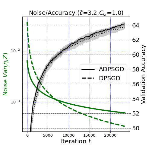
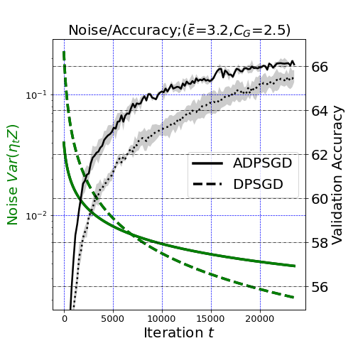
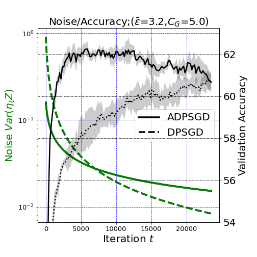
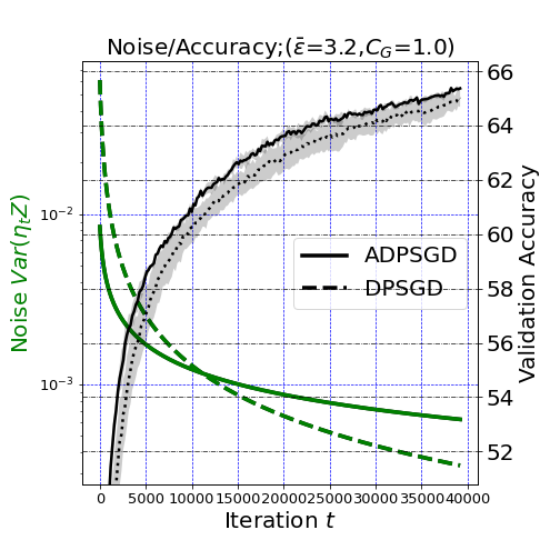
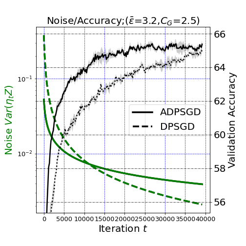
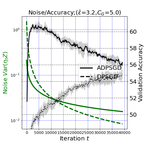
Figure 3: Validation accuracy with respect to iteration $t$ using ADP-SGD/DP-SGD with polynomially decaying stepsizes $\eta_{t}=\eta/b_{t+1}=1/\sqrt{20+t}$ (see the blue curve in Figure 2). The black lines corresponding to the right y-axis are measured by the validation accuracy on CIFAR10 for a CNN model using ADP-SGD (solid line) and DP-SGD (dash line). The shaded region is the one standard deviation. Each plot corresponds to a privacy budget $\bar{\varepsilon}=3.2$ with a fixed gradient clipping value $C_{G}$ (see title) and a fixed $T$ (see x-axis) where the top (bottom) row is for 120 (200) training epochs. Same as Figure 1, the monotone green curves, which correspond to the left vertical y-axis, show the actual noise for $\alpha_{t}=1/\sqrt{\eta_{t}}$ (ADP-SGD, the solid line) and $\alpha_{t}=1$ (DP-SGD, the dashed line). The top middle plot is the same as the right plot in Figure 1.

To further understand DP and ADP with respect to different privacy parameters and the gradient clipping values, we present the detailed performance in Figure 3 for $T=23520$ (120 epochs) where each plot corresponds to a pair of $(\bar{\varepsilon}=3.2,C_{G})$. We see that from Figure 3 that the gap between ADP-SGD and DP-SGD becomes more significant as $C_{G}$ increases from $1$ to $5$; ADP achieves the highest accuracy at $C_{G}=2.5$ with the best mean accuracy $66.41\%$. The intuition is that the noise added to the gradient with a large gradient clipping $C_{G}$ is much higher than that with a small gradient clipping value. In this situation, our method proves to be helpful by spreading out the total noise across the entire optimization process more evenly than DP-SGD (see the green curves in Figure 3). On the other hand, using a large gradient clipping $C_{G}=5$, our method suffers an over-fitting issue while DP-SGD performs considerably poorer. Thus one should be cautious when selecting the gradient clipping values $C_{G}$.

6.2 ADP-SGD v.s. DP-SGD for adaptive stepsizes

In this section, we focus on understanding the optimality of the theoretical guarantees of Proposition 5.2; we study the numerical performance of ADP-SGD with stepsizes updated by the gradients. We notice that, at the beginning of the training, the gradient norm in our model lies between $0.0001$ and $0.001$ when $C_{G}=1.0$. To remedy this small gradient issue, we let $b_{t}$ follow a more general form: $b^{2}_{t+1}=b^{2}_{t}+\max{\{\beta_{t}\|\nabla f(\theta_{t};x_{\xi_{t}})\|^{2},10^{-5}\}}$ with $\beta_{t}>1$. Specifically, we set $\beta_{t}=\max\{\beta/((t\mod 195)+1)),1\}$ with $\beta$ searching in a set $\{1,512,1024,2048,4096,8192\}$. See Section F.2 for a detailed description. As mentioned in Section 5.2, we set $\alpha_{t}^{2}=\sqrt{b_{0}^{2}+tC}$ in advance with $b_{0}^{2}=20$, and choose $C\in\{10^{-5},10^{-4},0.001,0.01,0.1,1\}$. We consider the number of iterations to be $T=11700$ with the gradient clipping $1.0$ and $2.5$. Table 3 summarizes the results of DP-SGD and ADP-SGD with the best hyper-parameters.

Table 3: Errors of ADP-SGD vs. DP-SGD with adaptive stepsizes. This table reports accuracy with the mean and the corresponding standard deviation over five independent runs. The value inside the bracket is the highest accuracy over the five runs. Each entry is the best value over 36 pairs of $(\beta,C)$ for ADP-SGD and 6 values of $\beta$ for DP-SGD. See the corresponding $(\beta,C)$ in Table 6. The results indicate that when using adaptive stepsizes, ADP-SGD with various $C$ performs better than DP-SGD.

$C_{G}$	Alg	$\bar{\varepsilon}=0.8$	$\bar{\varepsilon}=1.6$
$1.0$	ADP	$56.68\pm 0.646$ $(57.65)$	$62.09\pm 0.346$ $(62.57)$
	DP	$56.24\pm 0.535$ $(57.02)$	$62.02\pm 0.264$ $(62.33)$
$2.5$	ADP	$56.27\pm 0.174$ $(56.46)$	$62.38\pm 0.428$ $(62.86)$
	DP	$55.65\pm 0.448$ $(55.98)$	$62.23\pm 0.238$ $(62.62)$

$C_{G}$	Alg	$\bar{\varepsilon}=3.2$	$\bar{\varepsilon}=6.4$
$1.0$	ADP	$64.51\pm 0.100$ $(64.61)$	$67.75\pm 0.171$ $(67.91)$
	DP	$64.33\pm 0.329$ $(65.03)$	$67.42\pm 0.141$ $(67.7)$
$2.5$	ADP	$64.29\pm 0.408$ $(64.85)$	$67.55\pm 0.156$ $(67.77)$
	DP	$64.26\pm 0.140$ $(64.39)$	$66.23\pm 0.367$ $(66.62)$

7 Related work

Differentially private empirical risk minimization.

Differentially Private Empirical Risk Minimization (DP-ERM) has been widely studied over the past decade. Many algorithms have been proposed to solve DP-ERM including objective perturbation [Chaudhuri et al., 2011, Kifer et al., 2012, Iyengar et al., 2019], output perturbation [Wu et al., 2017, Zhang et al., 2017], and gradient perturbation [Bassily et al., 2014, Wang et al., 2017, Jayaraman and Wang, 2018]. While most of them focus on convex functions, we study DP-ERM with nonconvex loss functions. As most existing algorithms achieving differential privacy in ERM are based on the gradient perturbation [Bassily et al., 2014, Wang et al., 2017, 2019, Zhou et al., 2020a], we thus study gradient perturbation.

Non-constant stepsizes for SGD and DP-SGD.

To ease the difficulty of stepsize tuning, we could apply polynomially decaying stepsize schedules [Ge et al., 2019] or adaptive gradient methods that update the stepsize using the gradient information [Duchi et al., 2011, McMahan and Streeter, 2010]. We called them adaptive stepsizes to distinguish our adaptive deferentially private methods. These non-private algorithms update the stepsize according to the noisy gradients, and achieve favorable convergence behavior [Levy et al., 2018, Li and Orabona, 2019, Ward et al., 2019, Reddi et al., 2021].

Empirical evidence suggests that differential privacy with adaptive stepsizes could perform almost as well as – and sometimes better than – DP-SGD with well-tuned stepsizes. This results in a significant reduction in stepsize tuning efforts and also avoids the extra privacy cost [Bu et al., 2020, Zhou et al., 2020b, a]. Several works [Lee and Kifer, 2018, Koskela and Honkela, 2020] also studied the nonuniform allocation of the privacy budget for each iteration. However, Lee and Kifer [2018] only proposes a heuristic method and the purpose of Koskela and Honkela [2020] is to avoid the need for a validation set used to tune stepsizes. In this work, we emphasize the optimal relationship between the stepsize and the variance of the random noise, and aim to improve the utility guarantee of our proposed method.

8 Conclusion and future work

In this paper, we proposed an adaptive differentially private stochastic gradient descent method in which the privacy mechanisms can be optimally adapted to the choice of stepsizes at each round, and thus obtain improved utility guarantees over prior work. Our proposed method has not only strong theoretical guarantees but also superior empirical performance. Given high-dimensional settings with only a fixed privacy budget available, our approach with a decaying stepsize schedule shows an improvement in convergence by a magnitude $\mathcal{O}(d\log(T)\sqrt{T}/n^{2})$ or a factor with $\mathcal{O}(\log(T))$ relative to DP-SGD.

Note that the sequence $\{\alpha_{t}\}$ has to be fixed before the optimization process begins, as our method require that the variance $\sigma^{2}$ for some privacy budget $\varepsilon$ depends on the $\{\alpha_{t}\}$ (Theorem 4.1). However, our theorem suggests that the optimal choice of $\alpha_{t}$ depends on the stepsize (Theorem 4.2), meaning that we have to know the stepsizes a priori; this is not possible for those stepsizes updated on the fly, such as AdaGrad [Duchi et al., 2011] and Adam [Kingma and Ba, 2014]. Thus, one potential avenue of future work is to see whether $\{\alpha_{t}\}$ can be updated on the fly in line with AdaGrad and Adam while maintaining a predefined privacy budget $\varepsilon$. Other future directions can be related to examining more choices of $\alpha_{t}$ given $b_{t}$. As mentioned in the main text, the relation $\alpha_{t}^{2}=b_{t}$ is not the unique setting to achieve the improved utility guarantees. A thorough investigation on $\alpha_{t}$ and $b_{t}$ with various gradient clipping values would therefore be an interesting extension. Finally, our adaptive differential privacy is applied only to a simple first-order optimization; generalizing to variance-reduced or momentum methods is another potential direction.

Appendix A Privacy guarantees and convergence of DP-SGD

With the preliminaries given in Section 2, we will briefly summarize the analysis of privacy guarantees for the standard differentially private stochastic gradient descent (DP-SGD) described in Algorithm 1 with $\alpha_{t}=1,\forall t\in[T]$. To make our algorithm more general and suitable to the practice where we select $m<n$ samples instead of selecting a single sample for each iteration Goyal et al. [2017], Wang et al. [2020], we restate the DP-SGD algorithm with $m$ random samples in Algorithm 2. This $m$ is called size of mini-batch. Denote $\mathcal{B}_{i}=\{x_{i_{1}},\ldots,x_{i_{m}}\}$ for the $i$-th mini-batch where $\mathcal{B}_{i}\cap\mathcal{B}_{j}=\emptyset$ and each element in $\{i_{k}\}$ is chosen uniformly in $[n]$ without replacement. In our experiments, $m=256$ and $n=50000$ for CIFAR10 (see Section 6 for details). For the rest of this section, we focus on analysis of Algorithm 2.

Algorithm 2 DP-SGD with mini-batch size $m$

1:Input $\theta_{0},b_{0}$ and $\eta$, $m<n/2$.

2:for $t=1,\ldots,T$ do

3:     prepare mini-batches $\mathcal{B}_{1},\mathcal{B}_{2},\ldots,\mathcal{B}_{\lceil n/m\rceil}$ such that $\mathcal{B}_{i}\cap\mathcal{B}_{j}=\emptyset$ for $i\neq j$ and $|\mathcal{B}_{i}|=m$

4:     get $\xi_{t}\sim\text{Uniform}(1,...,\lceil n/m\rceil)$ and $c_{t}\sim\mathcal{N}(0,\sigma I)$

5:     update $b_{t+1}=\phi_{1}\left(b_{t},\frac{1}{|\mathcal{B}_{\xi_{t}}|}\sum_{i\in\mathcal{B}_{\xi_{t}}}\nabla f(\theta_{t};x_{i})\right)$

6:     release gradient $g^{b}_{t}=\frac{\eta}{b_{t+1}}(\frac{1}{|\mathcal{B}_{\xi_{t}}|}\sum_{i\in\mathcal{B}_{\xi_{t}}}\nabla f(\theta_{t};x_{i})+c_{t})$

7:     update $\theta_{t+1}=\theta_{t}-g^{b}_{t}$

8:end for

Theorem A.1 presented below has been well studied in prior work Bassily et al. [2014], Song et al. [2013], Wang et al. [2020]. We stated here for the completeness of the paper and to clarify the constant in the expression of $\sigma^{2}$.

Lemma A.1 (Privacy Amplification via Sampling Kasiviswanathan et al. [2011]).

Let the mechanism $\mathcal{M}:\mathcal{D}\to\mathcal{R}$ be $(\varepsilon,\delta)$-DP. Consider $\mathcal{M}_{q}$ follows the two steps (1) sample a random $q$ fraction of $\mathcal{D}$ (2) run $\mathcal{M}$ on the sample. Then the mechanism $\mathcal{M}_{q}$ is $((e^{\varepsilon}-1)q,q\delta)$-DP.

Lemma A.2 (Advanced Composition [Dwork et al., 2006a]).

For all $\varepsilon_{0},\delta_{0},\delta^{\prime}>0$, let $\mathcal{M}=(\mathcal{M}_{1},\ldots,\mathcal{M}_{k})$ be a sequence of $(\varepsilon_{0},\delta_{0})$-differentially private algorithms. Then, $\mathcal{M}$ is $(\varepsilon,\delta)$-differentially private, where $\varepsilon=\varepsilon_{0}\sqrt{2k\log(1/\delta^{\prime})}+k\varepsilon_{0}\frac{e^{\varepsilon_{0}}-1}{e^{\varepsilon_{0}}+1}$ and $\delta=1-(1-\delta_{0})^{k}+\delta^{\prime}$.

Theorem A.1 (Privacy Guarantee for DP-SGD).

Suppose the sequence $\{\alpha_{t}\}_{t=1}^{T}$ is all constant $1$ and that Assumption 2.2 holds. Algorithm 2 satisfies $(\varepsilon,\delta)$-DP if the random noise $c_{t}$ has variance

$$\sigma^{2} =\frac{(16G)^{2}B_{\delta}T}{n^{2}\varepsilon^{2}}\text{ with }B_{\delta}=\log(16Tm/n\delta))\log(1.25/\delta),$$ (13)

where $T\geq n^{2}\varepsilon^{2}B_{\delta}/(8m^{2}\log(1.25/\delta_{0}))$.

Proof.

The proof can be summarized into three steps Bassily et al. [2014]:

• Step One. By Assumption 2.2, the gradient sensitivity of the loss function is

  $$\Delta=\frac{1}{m}\sup_{x\in\mathcal{D},x\in\mathcal{D^{\prime}}}\left\|\nabla f(w;x)-\nabla f(w;x^{\prime})\right\|\leq 2G/m.$$

  Given the privacy budget $\varepsilon$, we apply Gaussian mechanism with $\sigma$ define in (13). By Lemma 2.1, the Gaussian privacy mechanism given in Definition 3.1 with $\alpha_{t}=1$ satisfies that $\varepsilon_{0}={2G/m\sqrt{2\log(1.25/\delta_{0})}}/{\sigma}$ for some $\delta_{0}\leq 10^{-5}$ such that $\delta_{0}Tm/n\ll 0.1$ Kamath [2020]. As we have $T\geq n^{2}\varepsilon^{2}B_{\delta}/(32m^{2}\log(1.25/\delta_{0}))$, the privacy

  $$\varepsilon_{0}^{2}={8G^{2}\log(1.25/\delta_{0})n^{2}\varepsilon^{2}}/({16^{2}G^{2}m^{2}B_{\delta}T})=n^{2}\varepsilon^{2}\log(1.25/\delta_{0})/(32m^{2}B_{\delta}T)\leq 1.$$

• Step Two. Applying amplification by sub-sampling (i.e. Lemma A.1), We have $(\varepsilon_{p},\delta_{p})-DP$ for each step in DP-SGD with $\varepsilon_{p}=2\varepsilon_{0}m/n\geq(e^{\varepsilon_{0}}-1)m/{n}$ and $\delta_{p}={\delta_{0}}m/{n}$, since $p=m/n<0.5$ and $\varepsilon_{0}\leq 1$.

• Step Three. After Step One and Two, we apply advanced (strong) composition stated in Lemma A.2 (Theorem III.3 Dwork et al. [2010] or Theorem 3.20 in Dwork et al. [2014]) for the $T$ iterations. Then, Algorithm 1 follows $(\varepsilon_{dpsgd},\delta_{dpsgd})$-DP satisfying for some $\delta^{\prime}$ such that $\delta_{0}Tm/(0.25n)\leq\delta^{\prime}\leq\delta_{0}Tm/(0.1n)\ll 1$.

  $$\delta_{dpsgd}= 1-(1-\delta_{0}m/n)^{T}+\delta^{\prime}\overset{(a)}{\leq}\delta_{0}Tm/n+\delta^{\prime}\leq 1.25\delta^{\prime}\leq 12.5\delta_{0}Tm/n,$$ (14)

  $$\varepsilon_{dpsgd}= \varepsilon_{p}\sqrt{2T\log(1/\delta^{\prime})}+T\varepsilon_{p}\frac{e^{\varepsilon_{p}}-1}{e^{\varepsilon_{p}}+1},$$ (15)

  where $(a)$ follows from the fact that $1-(1-\delta_{0}m/n)^{k}\leq\delta_{0}mk/n$. We now simplify (15)

  $$\varepsilon_{dpsgd}= \varepsilon_{p}\sqrt{2T\log(1/\delta^{\prime})}+T\varepsilon_{p}\frac{e^{\varepsilon_{p}}-1}{e^{\varepsilon_{p}}+1}$$

  $$\overset{(a)}{\leq} \varepsilon_{p}(\sqrt{2T\log({1}/{\delta^{\prime}})}+T\varepsilon_{p})$$

  $$\overset{(b)}{\leq} 2(2{\varepsilon_{0}}m/{n})\sqrt{2T\log({1}/{\delta^{\prime}})}$$

  $$\overset{(c)}{=} \frac{8mG/m\sqrt{2\log(\frac{1.25}{\delta_{0}})2T\log({1}/{\delta^{\prime}})}}{n\sigma}$$

  $$\overset{(d)}{\leq} \frac{16G\sqrt{T\log(16Tm/(n\delta_{dpsgd}))\log(1.25/\delta_{dpsgd})}}{n\sigma},$$

  where (a) follows from $({e^{\varepsilon_{p}}-1})/({e^{\varepsilon_{p}}+1})\leq\varepsilon_{p}(1+{\varepsilon_{p}})/(2+\varepsilon_{p})\leq\varepsilon_{p}$ as $1+{\varepsilon_{p}}\leq e^{\varepsilon_{p}}\leq 1+\varepsilon_{p}+\varepsilon_{p}^{2}$ for $\varepsilon_{p}<1$; (b) is due to that $T\varepsilon_{p}\leq\sqrt{2T\log(1/\delta^{\prime})}$ which is derived from

  $$T^{2}\varepsilon_{p}^{2}\leq\frac{T^{2}\varepsilon_{0}^{2}m^{2}}{n^{2}}\leq\frac{8T(G/m)^{2}m^{2}\log(1.25/\delta_{0})}{n^{2}\sigma^{2}}=T^{2}\frac{8G^{2}\log(1.25/\delta_{0})\varepsilon^{2}}{64G^{2}B_{\delta}T}\leq 2T\log(1/\delta^{\prime}),$$

  where the last inequality is from $\varepsilon^{2}\leq\frac{16\log(1/\delta^{\prime})B_{\delta}}{\log(1/\delta_{0})}$; (c) follows by substituting the $\varepsilon_{0}={2G\sqrt{2\log(1.25/\delta_{0})}}/{\sigma}$ given in Step One; (d) follows from the (14).

  Now we let $\delta_{dpsgd}=\delta$ and compare the relationship between $\varepsilon_{dpsgd}$ and $\varepsilon$:

  $$\varepsilon^{2}_{dpsgd} {\leq}\frac{(16G)^{2}{T\log(16Tm/(n\delta_{dpsgd}))\log(1.25/\delta_{dpsgd})}}{n^{2}\sigma^{2}}$$

  $$=\frac{(16G)^{2}{T\log(16Tm/(n\delta_{dpsgd}))\log(1.25/\delta_{dpsgd})}}{n^{2}}\frac{n^{2}\varepsilon^{2}}{(16G)^{2}B_{\delta}T}$$

  $$=\frac{\varepsilon^{2}\log(16Tm/(n\delta_{dpsgd}))\log(1.25/\delta_{dpsgd})}{\log(16Tm/(n\delta))\log(1.25/\delta)}$$

  $$\leq\varepsilon^{2}.$$

Thus, setting the $\sigma$ in Equation 13 is sufficient to obtain an $(\varepsilon,\delta)$-DP algorithm.

∎

Proposition A.1.

(DP-SGD with constant stepsizes) Under the conditions of Theorem 4.2 on $f$. Set $\sigma^{2}$ satisfying (13) in Theorem A.1. Let $b_{t}=1$ in Algorithm 2 and denote $\tau=\arg\min_{t\in[T-1]}\mathbb{E}[\|\nabla F(\theta_{t})\|^{2}]$ and $B_{\delta}=\log(16Tm/n\delta))\log(1.25/\delta)$. Then the gradients follow

$$\mathbb{E}[\|\nabla F(\theta_{\tau})\|^{2}]\leq\frac{2D_{F}}{\eta T}+\eta LG^{2}\left(1+d\frac{16^{2}B_{\delta}T}{n^{2}\varepsilon^{2}}\right).$$ (16)

We omit the proof of the proposition as it can be found in Wang et al. [2020]. In fact, the proof is strarightfoward by applying Theorem C.2 and noticing that

$$\|\frac{1}{m}\sum_{i\in\mathcal{B}}\nabla f(w;x_{i})\|^{2}\leq\frac{m}{m^{2}}\sum_{i\in\mathcal{B}}\|\nabla f(w;x_{i})\|^{2}\leq G^{2}.$$

Set $\eta=\sqrt{1/T}$, Equation 16 becomes

$$\mathbb{E}[\|\nabla F(\theta_{\tau})\|^{2}]\leq\frac{2D_{F}+LG^{2}}{\sqrt{T}}+\frac{L(16G)^{2}B_{\delta}\sqrt{T}}{n^{2}\varepsilon^{2}}.$$ (17)

Let us compare DP-SGDs between the constant stepsize $\eta/b_{t}=\sqrt{1/T}$ and the decaying stepsize $\eta/b_{t}=1/\sqrt{a+ct}$. Suppose the second term introduced by the privacy mechanism dominates the bound. We see that the ratio of second term in the bound using the decaying stepsize (i.e., Equation 26 in Proposition 5.1) to that using the constant stepsize (i.e., Equation 17) is $\mathcal{O}(\log(T)/\sqrt{c})$. Thus, if we set $\sqrt{c}=\log(T)$, the second term in both Equation 17 and Equation 26 have the same order.

Let us now compare between DP-SGD with the constant stepsize $\eta/b_{t}=\sqrt{1/T}$ and ADP-SGD with $\alpha_{t}^{2}=b_{t}$ and the decaying stepsize $\eta/b_{t}=1/\sqrt{a+ct}$. We have the ratio of second term in the bound Equation 26 to that in Equation 17) is $\mathcal{O}(1/\sqrt{c})$. Thus setting $\sqrt{c}=\log(T)$ in $\eta/b_{t}=1/\sqrt{a+ct}$ for ADP-SGD with $\alpha_{t}^{2}=b_{t}$ will results in a better utility bound than DP-SGD with $\eta/b_{t}=\sqrt{1/T}$.

From Equation 17, we see that setting $T_{\rm opt}=C_{1}(2D_{F}+LG^{2})n^{2}\varepsilon^{2}/(dLG^{2}\log(1/\delta))$ for some $C_{1}$ results in a tight bound. If we know the Lipschitz smoothness parameter $L$ for the function $F$ and the distance $D_{F}=F(\theta_{0})-F^{*}$, we could obtain the $T_{\rm opt}$. However, in practice, the Lipschitz smoothness $L$ and the distance $D_{F}$ are unknown values. Estimating these parameters has become an active research area Jordan and Dimakis [2020], Scaman and Virmaux [2018]. Thus we will not discuss about the optimal value of $T$ and think it is more reasonable to keep it in the bound.

Appendix B Proof for Extended Advanced Composition Theorem

We restate Lemma 2.2 as follows.

Lemma B.1 (Extended Advanced Composition).

Consider two sequences $\{\varepsilon_{i}\}_{i=1}^{k},\{\delta_{i}\}_{i=1}^{k}$ of positive numbers satisfying $\varepsilon_{i}\in(0,1)$ and $\delta_{i}\in(0,1)$. Let $\mathcal{M}_{i}$ be $(\varepsilon_{i},\delta_{i})$-differentially private for all $i\in\{1,2,\ldots,k\}$. Then $\mathcal{M}=(\mathcal{M}_{1},\ldots,\mathcal{M}_{k})$ is $(\tilde{\varepsilon},\tilde{\delta})$-differentially private for $\delta^{\prime}\in(0,1)$ and

$$\tilde{\varepsilon}=\sqrt{\sum_{i=1}^{k}2\varepsilon_{i}^{2}\log\left(\frac{1}{\delta^{\prime}}\right)}+\sum_{i=1}^{k}\frac{\varepsilon_{i}(e^{\varepsilon_{i}}-1)}{(e^{\varepsilon_{i}}+1)},\quad\quad\tilde{\delta}=1-(1-\delta_{1})(1-\delta_{2})\ldots(1-\delta_{k})+\delta^{\prime}.$$

The result follows immediately from Theorem 3.5 of Kairouz et al. [2017]. Alternative proof would be using Renyi DP. This result immediately follows by invoking Lemmas 2.6 and 2.7 of Feldman et al. [2020]. Particularly, Lemma 2.7 in Feldman et al. [2020]) gives a composition rule for Rényi differential privacy, which can then be used to obtain our version of composition for $(\epsilon,\delta)$-differential privacy. Lemma 2.6 in Feldman et al. [2020] allows translating Rényi differential privacy to $(\epsilon,\delta)$-differential privacy.

Appendix C Proof for Section 4

As explain in Appendix A, we we will select $m\leq n/2$ samples instead of selecting a single sample for each iteration. We restate Algorithm 1 in Algorithm 3 with mini-batches $m$ variable.

Algorithm 3 ADP-SGD with mini-batch size $m$

1:Input: $\theta_{0},b_{0},\alpha_{0}$, $\eta>0$ and $m\leq n/2$

2:for $t=0,1,\ldots,T-1$ do

3:     prepare mini-batches $\mathcal{B}_{1},\mathcal{B}_{2},\ldots,\mathcal{B}_{\lceil n/m\rceil}$ such that $\mathcal{B}_{i}\cap\mathcal{B}_{j}=\emptyset$ for $i\neq j$ and $|\mathcal{B}_{i}|=m$

4:     get $\xi_{t}\sim\text{Uniform}(1,...,\lceil n/m\rceil)$ and $c_{j}\sim\mathcal{N}(0,\sigma I)$

5:     update $b_{t+1}=\phi_{1}\left(b_{t},\frac{1}{|\mathcal{B}_{\xi_{t}}|}\sum_{i\in\mathcal{B}_{\xi_{t}}}\nabla f(\theta_{t};x_{i})\right)$

6:     update $\alpha_{t+1}=\phi_{2}(\alpha_{t},b_{t+1})$

7:     release $g^{b}_{t}=\frac{\eta}{b_{t+1}}\left(\frac{1}{|\mathcal{B}_{\xi_{t}}|}\sum_{i\in\mathcal{B}_{\xi_{t}}}\nabla f(\theta_{t};x_{i})+\alpha_{t+1}c_{j}\right)$

8:     update $\theta_{t+1}=\theta_{t}-g^{b}_{t}$

9:end for

C.1 Proof for Theorem 4.1

Let us restate Theorem 4.1 in Theorem C.1 for a mini-batch described in Algorithm 3.

Theorem C.1 (Privacy Guarantee).

Suppose the sequence $\{\alpha_{t}\}_{t=1}^{T}$ is known in advance and that Assumption 2.2 holds. Denote $B_{\delta}=\log(16Tm/n\delta))\log(1.25/\delta)$ as in Theorem A.1. Algorithm 3 with $m$ satisfies $(\varepsilon,\delta)$-DP if the random noise $c_{j}$ has variance

$$\sigma^{2} =\frac{(16G)^{2}B_{\delta}}{n^{2}\varepsilon^{2}}\;{\sum_{t=0}^{T-1}\frac{1}{\alpha^{2}_{t+1}}},$$ (18)

where $T$ is required to satisfy $\alpha_{t}^{2}\sum_{t=1}^{T}1/\alpha^{2}_{t}\geq n^{2}\varepsilon^{2}B_{\delta}/(32m^{2}\log(1.25/\delta_{0}))$.

Proof.

Similar to the proof in Theorem A.1, we will follow three steps.

• Step One. At $t$ iteration, the Gaussian privacy mechanism given in Definition 3.1 with any $\alpha_{t}$ satisfies that $(\varepsilon_{t},\delta_{0})-$DP where $\varepsilon_{t}={2G/m\sqrt{2\log(1.25/\delta_{0})}}/{(\alpha_{t}\sigma)}$ for some $\delta_{0}\ll 10^{-5}$ such that $\delta_{0}T/n\ll 0.1$. Note that the privacy

  $$(\varepsilon_{p}^{t})^{2} =\frac{8G^{2}\log(1.25/\delta_{0})}{\alpha_{t}^{2}m^{2}}\frac{n^{2}\varepsilon^{2}}{(16G)^{2}B_{\delta}\sum_{t=1}^{T}1/\alpha_{t}^{2}}$$ (19)

  $$=n^{2}\varepsilon^{2}\log(1.25/\delta_{0})/(32m^{2}B_{\delta}\alpha_{t}^{2}\sum_{t=1}^{T}1/\alpha_{t}^{2})\leq 1,$$ (20)

  where the last inequality is due to the fact that $\alpha_{t}^{2}\sum_{t=1}^{T}1/\alpha^{2}_{t}\geq n^{2}\varepsilon^{2}B_{\delta}/(32\log(1.25/\delta_{0}))$.

• Step Two. Applying amplification by sub-sampling (i.e. Lemma A.1), We have $(\varepsilon^{t}_{p},\delta_{p})$-DP for each step in DP-SGD with $\varepsilon^{t}_{p}=2\varepsilon_{t}m/n\geq(e^{\varepsilon_{t}}-1)m/{n}$ and $\delta_{p}={\delta_{0}}m/{n}$, since $p=m/n$ and $\varepsilon_{t}\leq 1$.

• Step Three. Using Lemma 2.2 or Lemma B.1, we have Algorithm 1 satisfying $(\varepsilon_{adpsgd},\delta_{adpsgd})$-DP for some $\delta^{\prime}$ such that $\delta_{0}Tm/(0.25n)\leq\delta^{\prime}\leq\delta_{0}Tm/(0.1n)\ll 1$.

  $$\delta_{adpsgd} =1-(1-\delta_{0}m/n)^{T}+\delta^{\prime}\leq\delta_{0}Tm/n+\delta^{\prime}\leq 1.25\delta^{\prime}\leq 12.5\delta_{0}Tm/n,$$ (21)

  $$\varepsilon_{adpsgd} =\sqrt{\sum_{t=1}^{T}2(\varepsilon_{p}^{t})^{2}\log\left(\frac{1}{\delta^{\prime}}\right)}+\sum_{t=1}^{T}\frac{\varepsilon^{t}_{p}(e^{\varepsilon_{p}^{t}}-1)}{(e^{\varepsilon_{p}^{t}}+1)}\overset{(a)}{\leq}2\sqrt{2\sum_{t=1}^{T}(\varepsilon_{p}^{t})^{2}\log\left(\frac{1}{\delta^{\prime}}\right)},$$ (22)

  where (a) is due to that $\sum_{t=1}^{T}\frac{\varepsilon^{t}_{p}(e^{\varepsilon_{p}^{t}}-1)}{(e^{\varepsilon_{p}^{t}}+1)}$ is considerable smaller than $\sqrt{\sum_{t=1}^{T}(\varepsilon_{p}^{t})^{2}\log\left(\frac{1}{\delta^{\prime}}\right)}$. Indeed,

  $$\sum_{t=1}^{T}\frac{\varepsilon^{t}_{p}(e^{\varepsilon_{p}^{t}}-1)}{(e^{\varepsilon_{p}^{t}}+1)} \leq\sum_{t=1}^{T}(\varepsilon^{t}_{p})^{2}=\frac{4m^{2}}{n^{2}}\sum_{t=1}^{T}\varepsilon_{t}^{2}=\frac{32G^{2}\log(1.25/\delta_{0})}{n^{2}\sigma^{2}}\sum_{t=1}^{T}\frac{1}{\alpha_{t}^{2}}=\frac{\log(1.25/\delta_{0})\varepsilon^{2}}{8B_{\delta}},$$

  $$\sqrt{\sum_{t=1}^{T}(\varepsilon_{p}^{t})^{2}\log\left(\frac{1}{\delta^{\prime}}\right)} =\sqrt{\frac{\log(1.25/\delta_{0})\varepsilon^{2}}{8B_{\delta}}\log\left(\frac{1}{\delta^{\prime}}\right)}\overset{(a)}{\geq}\frac{\log(1.25/\delta_{0})\varepsilon^{2}}{8B_{\delta}}\geq\sum_{t=1}^{T}\frac{\varepsilon^{t}_{p}(e^{\varepsilon_{p}^{t}}-1)}{(e^{\varepsilon_{p}^{t}}+1)},$$

  where (a) is due to the fact that $\frac{\log(1.25/\delta_{0})\varepsilon^{2}}{8\log({1}/{\delta^{\prime}})B_{\delta}}<1$. Let $\delta_{adpsgd}=\delta$. We now further simply $\varepsilon_{adpsgd}$ as follows

  $$\varepsilon_{adpsgd}^{2}\leq 8\log\left({1}/{\delta^{\prime}}\right)\sum_{t=1}^{T}(\varepsilon_{p}^{t})^{2}=\frac{\log\left({1}/{\delta^{\prime}}\right)\log(1.25/\delta_{0})\varepsilon^{2}}{B_{\delta}}\overset{(a)}{\leq}\varepsilon^{2},$$

  where the last step (a) is due to Equation 21.

∎

C.2 Proof for Theorem 4.2

We restate Theorem C.2 with the following theorem for a mini-batch described in Algorithm 3.

Theorem C.2 (Convergence for ADP-SGD).

Suppose we choose $\sigma^{2}$ - the variance of the random noise in Algorithm 3 - according to (18) in Theorem C.1. Suppose Assumption 2.1, 2.2 and 3.1 hold. Furthermore, suppose $\alpha_{t},b_{t}$ are deterministic. The utility guarantee of Algorithm 3 with $\tau\triangleq\text{arg}\min_{k\in{[T-1]}}\mathbb{E}[\|\nabla F(\theta_{k})\|^{2}]$ and $B_{\delta}=\log(16Tm/n\delta))\log(1.25/\delta)$ is

$$\mathbb{E}\|\nabla F(\theta_{\tau})\|^{2} \leq\frac{1}{\sum_{t=0}^{T-1}\frac{1}{b_{t+1}}}\left(\frac{D_{F}}{\eta}+\frac{\eta L}{2}\sum_{t=0}^{T-1}\frac{\mathbb{E}\left[\|g_{\xi_{t}}\|^{2}\right]}{b^{2}_{t+1}}+\frac{d(16G)^{2}B_{\delta}}{2n^{2}\varepsilon^{2}}M\right),$$ (23)

where

$$g_{\xi_{t}}=\frac{1}{|\mathcal{B}_{\xi_{t}}|}\sum_{i\in\mathcal{B}_{\xi_{t}}}\nabla f(\theta_{t};x_{i})\text{ and }M(\{\alpha_{t}\},\{b_{t}\}){\triangleq}\textstyle\sum_{t=0}^{T-1}(\alpha_{t+1}/b_{t+1})^{2}\sum_{t=1}^{T-1}1/\alpha^{2}_{t+1}.$$

Proof.

Recall the update in Algorithm 1:

$$\theta_{t+1} =\theta_{t}-\frac{\eta}{b_{t+1}}g_{\xi_{j}}-\eta\frac{\alpha_{t+1}}{b_{t+1}}c_{j}.$$

By Lipschitz gradient smoothness (c.f. Lemma E.1):

$$F(\theta_{j+1}) \leq F(\theta_{j})-\eta\langle{\nabla F(\theta_{j}),\frac{1}{b_{j+1}}g_{\xi_{j}}-\frac{\alpha_{j+1}}{b_{j+1}}c_{j}\rangle}+\frac{\eta^{2}L}{2}\left\|\frac{g_{\xi_{j}}}{b_{j+1}}+\frac{\alpha_{j+1}}{b_{j+1}}c_{j}\right\|^{2},$$

$$\mathbb{E}[F(\theta_{j+1})] \leq\mathbb{E}[F(\theta_{j})]+\mathbb{E}\left[\frac{-\eta}{b_{j+1}}\langle{\nabla F(\theta_{j}),g_{\xi_{j}}\rangle}+\frac{\eta^{2}L}{2b_{j+1}^{2}}\|g_{\xi_{j}}\|^{2}+\frac{\eta^{2}dL\sigma^{2}}{2}\frac{\alpha^{2}_{j+1}}{b_{j+1}^{2}}\right].$$

So we have by telescoping from $j=0$ to $j=T-1$

$$\mathbb{E}[F(\theta_{T-1})]\leq\mathbb{E}[F(\theta_{0})]+\sum_{j=0}^{T-1}\mathbb{E}\left[\frac{-\eta}{b_{j+1}}\langle{\nabla F(\theta_{j}),g_{\xi_{j}}\rangle}+\frac{\eta^{2}L}{2b_{j+1}^{2}}\|g_{\xi_{j}}\|^{2}+\frac{\eta^{2}dL\sigma^{2}}{2}\frac{\alpha^{2}_{j+1}}{b_{j+1}^{2}}\right].$$

Moving the term $\sum_{j=0}^{T-1}\mathbb{E}\left[\frac{-\eta}{b_{j+1}}\langle{\nabla F(\theta_{j}),g_{\xi_{j}}\rangle}\right]$ to the left hand side gives

$$\sum_{j=0}^{T-1}\mathbb{E}\left[\frac{\langle{\nabla F(\theta_{j}),g_{\xi_{j}}\rangle}}{b_{j+1}}\right] \leq\frac{D_{F}}{\eta}+\frac{\eta L}{2}\mathbb{E}\left[\sum_{t=0}^{T-1}\frac{\|g_{\xi_{t}}\|^{2}]}{b^{2}_{t+1}}+\frac{d\sigma^{2}}{2}\sum_{t=0}^{T-1}\left(\frac{\alpha_{t+1}}{b_{t+1}}\right)^{2}\right]$$

$$\overset{(a)}{=}\frac{D_{F}}{\eta}+\frac{\eta L}{2}\sum_{t=0}^{T-1}\mathbb{E}\left[\frac{\|g_{\xi_{t}}\|^{2}}{b^{2}_{t+1}}\right]+\frac{\eta dL(16G)^{2}B_{\delta}M}{2n^{2}\varepsilon^{2}},$$

where (a) follows by substituting $\sigma$ with (18) and denoting $M=\sum_{t=0}^{T-1}\frac{\alpha^{2}_{t+1}}{b^{2}_{t+1}}\sum_{t=0}^{T-1}\frac{1}{\alpha^{2}_{t+1}}.$ We finish the proof by simplifying the left hand side in above inequality as follows

$$\sum_{j=0}^{T-1}\mathbb{E}\left[\frac{\langle{\nabla F(\theta_{j}),g_{\xi_{j}}\rangle}}{b_{j+1}}\right]\geq\sum_{j=0}^{T-1}\frac{\mathbb{E}\left[\|\nabla F(\theta_{j})\|^{2}\right]}{b_{j+1}}\geq\min_{j\in{[T-1]}}\mathbb{E}\left[\|\nabla F(\theta_{j})\|^{2}\right]\sum_{j=0}^{T-1}\frac{1}{b_{j+1}}.$$ (24)

∎

Now let us take a look at the Remark 4.1. For $M$, note that

$$M=\sum_{t=0}^{T-1}\frac{\alpha^{2}_{t+1}}{b^{2}_{t+1}}\sum_{t=0}^{T-1}\frac{1}{\alpha^{2}_{t+1}} \geq\left(\sum_{t=0}^{T-1}\sqrt{\frac{\alpha^{2}_{t+1}}{b^{2}_{t+1}}}\sqrt{\frac{1}{\alpha^{2}_{t+1}}}\right)^{2}=\left(\sum_{t=0}^{T-1}\frac{1}{b_{t+1}}\right)^{2}=M_{\rm adp},$$

where we apply the fact that $\|w\|^{2}\|v\|^{2}\geq|\langle{w,v\rangle}|^{2}$ and the equality holds when $\frac{\alpha_{t+1}}{b_{t+1}}=\frac{1}{\alpha_{t+1}}$. So the optimal relationship for $t=1,2,\ldots,T$ is $\alpha^{2}_{t}=b_{t}.$ On the other hand, observe that

$$M=\sum_{t=0}^{T-1}\frac{\alpha^{2}_{t+1}}{b^{2}_{t+1}}\sum_{t=0}^{T-1}\frac{1}{\alpha^{2}_{T-1-t}} \overset{(a)}{\geq}\left(\sum_{t=0}^{T-1}\sqrt{\frac{\alpha^{2}_{t+1}}{b^{2}_{t+1}}}\sqrt{\frac{1}{\alpha^{2}_{T-1-t}}}\right)^{2}=\left(\sum_{t=0}^{T-1}\frac{1}{b_{t+1}}\right)^{2}=M_{\rm adp},$$

where the equality in (a) holds if $\alpha_{t}\alpha_{T-(t-1)}=b_{t}$.

Appendix D Proofs for Section 5

For this section, we restate the Proposition 5.1 with Proposition D.1 for a more general setup – Algorithm 3 with a mini-batch of size $m$.

Proposition D.1 (ADP-SGD v.s. DP-SGD with a polynomially decaying stepsize schedule).

Under the conditions of Theorem C.2 on $f$ and $\sigma^{2}$, let $b_{t}=(a+ct)^{1/2}$ in Algorithm 3, where $a>0,c>0$. Denote $\tau=\arg\min_{t\in[T-1]}\mathbb{E}[\|\nabla F(\theta_{t})\|^{2}]$, $B_{\delta}=\log(16Tm/n\delta))\log(1.25/\delta)$ and $B_{T}=\log\left(1+T{c}/{a}\right)$. If we choose $T\geq 5+4{a}/{c}$, and $\alpha_{t}^{2}=b_{t}$, we have the following utility guarantee for ADP-SGD

$$\textbf{(ADP-SGD)}\quad\mathbb{E}[\|\nabla F(\theta_{\tau}^{\rm ADP})\|^{2}] \leq\frac{\sqrt{c}\left(\frac{D_{F}}{\eta}+\frac{\eta G^{2}LB_{T}}{2c}\right)}{\sqrt{T-1}}+\frac{\eta dL(16G)^{2}B_{\delta}\sqrt{T}}{n^{2}\varepsilon^{2}\sqrt{c}}.$$ (25)

In addition, if we choose $T\geq 5+4{a}/{c}$ and $\alpha_{t}=1$, we have the utility guarantee for DP-SGD:

$$\textbf{(DP-SGD)}\quad\mathbb{E}[\|\nabla F(\theta_{\tau}^{\rm DP})\|^{2}] \leq\frac{\sqrt{c}\left(\frac{D_{F}}{\eta}+\frac{\eta G^{2}LB_{T}}{2c}\right)}{\sqrt{T-1}}+\frac{\eta dL(16G)^{2}B_{\delta}B_{T}(\sqrt{T-1}+1)}{2n^{2}\varepsilon^{2}\sqrt{c}}.$$ (26)

Proof.

The proof will be divided into two parts: Section D.1 is for ADP-SGD and Section D.2 is for DP-SGD.

D.1 Proof for Proposition D.1 – ADP-SGD with $b_{t}=\sqrt{a+ct}$

Note from Lemma E.2 we have

$$\frac{2}{\sqrt{c}}\left(\sqrt{\frac{a}{c}+T}-\sqrt{\frac{a}{c}+1}\right)\leq\sum_{j=0}^{T-1}\frac{1}{b_{j+1}}=\sum_{j=1}^{T}\frac{1}{\sqrt{a+ct}}\leq\frac{2}{\sqrt{c}}\left(\sqrt{\frac{a}{c}+T}-\sqrt{\frac{a}{c}}\right).$$ (27)

Set $\widetilde{B_{1}}=\mathbb{E}\left[\sum_{t=0}^{T-1}\frac{\|g_{\xi_{t}}\|^{2}}{b^{2}_{t+1}}\right]$. Continue with the bound Equation 23 of Theorem C.2 with $\alpha_{t}^{2}=b_{t}$

$$\mathbb{E}\|\nabla F(\theta_{\tau})\|^{2} \leq\frac{L}{\sum_{\ell=0}^{T-1}\frac{1}{b_{\ell+1}}}\left(\frac{D_{F}}{\eta L}+\frac{\eta}{2}\sum_{\ell=0}^{T-1}\frac{\mathbb{E}[\|g_{\xi_{\ell}}\|^{2}]}{b^{2}_{\ell+1}}\right)+\frac{\eta dL(16G)^{2}B_{\delta}}{2n^{2}\varepsilon^{2}}\left(\sum_{\ell=0}^{T-1}\frac{1}{b_{\ell+1}}\right)$$

$$\overset{(a)}{\leq}\frac{D_{F}/{\eta}+\eta L\widetilde{B_{1}}/2}{\frac{2}{\sqrt{c}}\left(\sqrt{\frac{a}{c}+T}-\sqrt{\frac{a}{c}+1}\right)}+\frac{\eta dL(16G)^{2}B_{\delta}}{2n^{2}\varepsilon^{2}}\left(\frac{2}{\sqrt{c}}\left(\sqrt{\frac{a}{c}+T}-\sqrt{\frac{a}{c}}\right)\right)$$

$$\overset{(b)}{\leq}\frac{\sqrt{a+{c}T}+\sqrt{a+c}}{2(T-1)}\left(\frac{D_{F}}{\eta}+\frac{\eta L\widetilde{B_{1}}}{2}\right)+\frac{\eta dL(16G)^{2}B_{\delta}}{n^{2}\varepsilon^{2}}\frac{2\sqrt{T}}{\sqrt{c}}$$

$$\overset{(c)}{\leq}\frac{\sqrt{c}}{\sqrt{T-1}}\left(\frac{D_{F}}{\eta}+\frac{\eta L\widetilde{B_{1}}}{2}\right)+\frac{\eta dL(16G)^{2}B_{\delta}\sqrt{T}}{n^{2}\varepsilon^{2}\sqrt{c}}$$

$$\overset{(d)}{\leq}\frac{\sqrt{c}}{\sqrt{T-1}}\left(\frac{D_{F}}{\eta}+\frac{\eta G^{2}LB_{T}}{2c}\right)+\frac{\eta dL(16G)^{2}B_{\delta}\sqrt{T}}{n^{2}\varepsilon^{2}\sqrt{c}},$$

where (a) is by replacing $\alpha_{t}^{2}=b_{t}$ in $M$; (b) follows by the fact that

$$\frac{2}{\sqrt{c}}\left(\sqrt{\frac{a}{c}+T}-\sqrt{\frac{a}{c}+1}\right)=\frac{2(T-1)}{\sqrt{a+{c}T}+\sqrt{a+c}}\quad\text{and}\quad\sqrt{\frac{a}{c}+T}-\sqrt{\frac{a}{c}}\leq\sqrt{T},$$

(c) is true due to the fact that $\frac{\sqrt{a+{T}{c}}+\sqrt{a+c}}{T-1}\leq\frac{2\sqrt{a+c}}{T-1}+\frac{\sqrt{c}}{\sqrt{T-1}}\leq\frac{2\sqrt{c}}{\sqrt{T-1}}$ as $T\geq 5+4\frac{a}{c}$; (6) with $B_{T}=\log\left(1+T{c}/{a}\right)$ is due to

$$\widetilde{B_{1}}=\mathbb{E}\left[\sum_{t=0}^{T-1}\frac{\|g_{\xi_{t}}\|^{2}}{a+c(t+1)}\right]\leq\sum_{t=0}^{T-1}\frac{G^{2}}{a+c(t+1)}\leq\frac{G^{2}}{c}\log\left(1+\frac{cT}{a}\right)=G^{2}B_{T}/c,$$

where we use Lemma E.2 with $p=1$.

D.2 Proof for Proposition D.1 – DP-SGD with $b_{t}=\sqrt{a+ct}$

Applying the fact in (24), (27), and that $\|g_{\xi_{t}}\|^{2}\leq G^{2}$, the bound Equation 23 of Theorem C.2 with $\alpha_{t}^{2}=1$ reduces to

$$\min_{k\in{[T-1]}}\mathbb{E}\|\nabla F(\theta_{k})\|^{2} \overset{(b)}{\leq}\frac{\sqrt{a+{c}T}+\sqrt{a+c}}{2(T-1)}\left(\frac{D_{F}}{\eta}+\frac{\eta LG^{2}B_{T}}{2c}+\frac{\eta dL(16G)^{2}T}{2cn^{2}\varepsilon^{2}}B_{\delta}B_{T}\right)$$

$$\overset{(c)}{\leq}\frac{\sqrt{c}}{\sqrt{T-1}}\left(\frac{D_{F}}{\eta}+\frac{\eta LG^{2}B_{T}}{2c}\right)+\frac{\eta dL(16G)^{2}}{2n^{2}\varepsilon^{2}\sqrt{c}}B_{\delta}B_{T}\frac{T}{\sqrt{T-1}},$$

where (a) is by Lemma E.2 (see (24)); (b) follows by substituting $\sigma$ and setting $B_{T}=\log\left(1+T\frac{c}{a}\right)$; (c) is true due to $\frac{\sqrt{a+{T}{c}}+\sqrt{a+c}}{T-1}\leq\frac{2\sqrt{a+c}}{T-1}+\frac{\sqrt{c}}{\sqrt{T-1}}\leq\frac{2\sqrt{c}}{\sqrt{T-1}}$ as $T\geq 5+4\frac{a}{c}$. ∎

D.3 Convergence for an adaptive stepsize schedule

Theorem D.1 (Convergence for an adaptive stepsize schedule).

Under the conditions of Theorem C.2 on $f$ and $\sigma^{2}$, let $b^{2}_{t+1}=b^{2}_{t}+\max{\left\{\frac{1}{|\mathcal{B}_{\xi_{j}}|}\|\sum_{i\in\mathcal{B}_{\xi_{j}}}\nabla f(\theta_{t};x_{i})\|^{2},\nu\right\}},\nu\in(0,G]$ in Algorithm 3. Denote $B_{\delta}=\log(16Tm/n\delta))\log(1.25/\delta)$ and $\tau=\arg\min_{t\in[T-1]}\mathbb{E}[\|\nabla F(\theta_{t})\|^{2}]$. If $T\geq 5+4b^{2}_{0}/G^{2}$, then the utility guarantee follows

$$\mathbb{E}[\|\nabla F(\theta_{\tau})\|^{2}] \leq\frac{2G}{\sqrt{T-1}}\left(B_{\rm sgd}+\frac{\eta dL(16G)^{2}B_{\delta}\mathbb{E}\left[M\right]}{2n^{2}\varepsilon^{2}}\right),$$

where $\displaystyle B_{\rm sgd}=\frac{D_{F}}{\eta}+\left(2G+\frac{\eta L}{2}\right)\left(1+\log\left(\frac{T(G^{2}+\nu^{2})}{b_{0}^{2}}+1\right)\right)$ and $\displaystyle M=\sum_{t=0}^{T-1}\frac{\alpha^{2}_{t+1}}{b^{2}_{t+1}}\sum_{t=1}^{T-1}\frac{1}{\alpha^{2}_{t+1}}$.

When $\alpha_{t}=0$, Proposition 5.1 (result in (25) with $M=0$) and Theorem D.1 (with $M=0$) corresponds to the standard SGD algorithms with decaying and adaptive stepsizes, respectively. In particular, if we set $a=b_{0}^{2}$, $c=G^{2}$ and $\alpha_{t}=0$ in Proposition 5.1, then the result in Proposition 5.1 becomes ${G\left({D_{F}}/{\eta}+{\eta G^{2}LB_{T}}/{2c}\right)}/{\sqrt{T-1}}\overset{\Delta}{=}Q_{\rm decay}$, while the result in Theorem D.1 is $2GB_{\rm sgd}/{\sqrt{T-1}}\overset{\Delta}{=}Q_{\rm adapt}$. We see that for a sufficiently large $G>L$, the advantage of using this variant of adaptive stepsizes is that $Q_{\rm adapt}=\mathcal{O}(G^{2}\log(T))/\sqrt{T})$ is smaller than $Q_{\rm decay}=\mathcal{O}(G^{3}\log(T))/\sqrt{T})$ by an order of $G$. Note that the proof follows closely with Ward et al. [2019].

Proof.

Write $F_{j}=F(\theta_{j})$ and $g_{\xi_{j}}=\frac{1}{|\mathcal{B}_{\xi_{j}}|}\sum_{i\in\mathcal{B}_{\xi_{j}}}\nabla f(\theta_{t};x_{i})$ . In addition, we write $\mathbb{E}_{j}[\cdot]$ means taking expectation with respect to the randomness of $\xi_{j}$ and $c_{j}$ conditional on $\{\xi_{t}\}_{t=0}^{j-1}$ and $\{c_{t}\}_{t=0}^{j-1}$; $\mathbb{E}_{c_{j}}[\cdot]$ means taking expectation with respect to the randomness of $c_{j}$ conditional on $\{\xi_{t}\}_{t=0}^{j-1}$ and $\{c_{t}\}_{t=0}^{j-1}$; $\mathbb{E}_{\xi_{j}}[\cdot]$ means taking expectation with respect to the randomness of $\xi_{j}$ conditional on $\{\xi_{t}\}_{t=0}^{j-1}$ and $\{c_{t}\}_{t=0}^{j-1}$. Note that since $c_{j}$ and $\xi_{j}$ is independent, thus we have $\mathbb{E}_{j}[\cdot]=\mathbb{E}_{c_{j}}[\cdot]\mathbb{E}_{\xi_{j}}[\cdot]$.

By Decent Lemma E.1,

$$F_{j+1} \leq F_{j}-\frac{\eta}{b_{j+1}}\langle{\nabla F_{j},g_{\xi_{j}}+\alpha_{j+1}c_{j}\rangle}+\frac{\eta^{2}L}{2b^{2}_{j+1}}\|g_{\xi_{j}}+\alpha_{j+1}c_{j}\|^{2}$$

$$=F_{j}-\frac{\eta\|\nabla F_{j}\|^{2}}{b_{j+1}}+\frac{\eta}{b_{j+1}}\langle{\nabla F_{j},\nabla F_{j}-g_{\xi_{j}}\rangle}-\frac{\eta\alpha_{j+1}}{b_{j+1}}\langle{\nabla F_{j},c_{j}\rangle}$$

$$\quad+\frac{\eta^{2}L\alpha_{j+1}}{b^{2}_{j+1}}\langle{g_{\xi_{j}},c_{j}\rangle}+\frac{\eta^{2}L\alpha^{2}_{j+1}}{2b^{2}_{j+1}}\|c_{j}\|^{2}+\frac{\eta^{2}L}{2b^{2}_{j+1}}\|g_{\xi_{j}}\|^{2}.$$ (28)

Observe that taking expectation with respect to $c_{j}$, conditional on $\xi_{1},\dots,\xi_{j-1},\xi_{j}$ gives

$$\mathbb{E}_{c_{j}}\left[\langle{\nabla g_{\xi_{j}},c_{j}\rangle}\right]=0\quad\mathbb{E}_{c_{j}}\left[\langle{\nabla F_{j},c_{j}\rangle}\right] =0\text{ and }\mathbb{E}_{c_{j}}\left[\|c_{j}\|^{2}\right]=d\sigma^{2}.$$ (29)

Thus, we have

$$\mathbb{E}_{c_{j}}\left[F_{j+1}\right] \leq F_{j}-\frac{\eta\|\nabla F_{j}\|^{2}}{b_{j+1}}+\frac{\eta}{b_{j+1}}\langle{\nabla F_{j},\nabla F_{j}-g_{\xi_{j}}\rangle}+\frac{\eta^{2}L}{2b^{2}_{j+1}}\left(\|g_{\xi_{j}}\|^{2}+\alpha^{2}_{j+1}d\sigma^{2}\right).$$ (30)

Note that taking expectation of $\frac{1}{b_{j}+G}\langle{\nabla F_{j},\nabla F_{j}-g_{\xi_{j}}\rangle}$ with respect to $\xi_{j}$ conditional on $\xi_{1},c_{1},\dots,\xi_{j-1},c_{j-1}$ gives

$$\mathbb{E}_{\xi_{j}}\left[\frac{1}{b_{j}+G}\langle{\nabla F_{j},\nabla F_{j}-g_{\xi_{j}}\rangle}\right] =\frac{1}{b_{j}+G}\mathbb{E}_{\xi_{j}}\left[\langle{\nabla F_{j},\nabla F_{j}-g_{\xi_{j}}\rangle}\right]=0.$$ (31)

Applying above inequalities back to the inequality 30 becomes

$$\mathbb{E}_{j}\left[\frac{F_{j+1}}{\eta}\right] \leq\frac{F_{j}}{\eta}-\frac{\|\nabla F_{j}\|^{2}}{b_{j}+G}+\mathbb{E}_{\xi_{j}}\left[\left(\frac{1}{b_{j}+G}-\frac{1}{b_{j+1}}\right)\langle{\nabla F_{j},g_{\xi_{j}}\rangle}\right]+\frac{\eta L}{2}\mathbb{E}_{\xi_{j}}\left[\frac{\|g_{\xi_{j}}\|^{2}+d\alpha^{2}_{j+1}\sigma^{2}}{b^{2}_{j+1}}\right].$$ (32)

Observe the identity

$$\frac{1}{b_{j}+G}-\frac{1}{b_{j+1}}=\frac{\max{\{\|g_{\xi_{j}}\|^{2},\nu\}}}{b_{j+1}(b_{j}+G)(b_{j}+b_{j+1})}-\frac{G}{b_{j+1}(b_{j}+G)};$$

thus, applying Cauchy-Schwarz,

$$\left(\frac{1}{b_{j}+G}-\frac{1}{b_{j+1}}\right)\langle{\nabla F_{j},g_{\xi_{j}}\rangle} =\left(\frac{\max{\{\|g_{\xi_{j}}\|^{2},\nu\}}}{b_{j+1}(b_{j}+G)(b_{j+1}+b_{j})}-\frac{G}{b_{j+1}(b_{j}+G)}\right)\langle{\nabla F_{j},g_{\xi_{j}}\rangle}$$

$$\leq\frac{\max{\{\|g_{\xi_{j}}\|^{2},\nu\}}\|g_{\xi_{j}}\|\|\nabla F_{j}\|}{b_{j+1}(b_{j+1}+b_{j})(b_{j}+G)}+\frac{G|\langle{\nabla F_{j},g_{\xi_{j}}\rangle}|}{b_{j+1}(b_{j}+G)}$$

$$\leq\frac{\sqrt{\max{\{\|g_{\xi_{j}}\|^{2},\nu\}}}\|g_{\xi_{j}}\|\|\nabla F_{j}\|}{(b_{j+1}+b_{j})(b_{j}+G)}+\frac{G\|\nabla F_{j}\|\|g_{\xi_{j}}\|}{b_{j+1}(b_{j}+G)}.$$ (33)

By applying the inequality $ab\leq\frac{\lambda}{2}a^{2}+\frac{1}{2\lambda}b^{2}$ with $\lambda=\frac{2G^{2}}{b_{j}+G}$, $a=\frac{\|g_{\xi_{j}}\|}{b_{j}+b_{j+1}}$, and $b=\frac{\|\nabla F_{j}\|\|g_{\xi_{j}}\|}{(b_{j}+G)}$, the first term in (33) can be bounded as

$$\mathbb{E}_{\xi_{j}}\frac{\sqrt{\max{\{\|g_{\xi_{j}}\|^{2},\nu\}}}\|g_{\xi_{j}}\|\|\nabla F_{j}\|}{(b_{j}+b_{j+1})(b_{j}+G)} \leq\mathbb{E}_{\xi_{j}}\frac{G^{2}}{(b_{j}+G)}\frac{\max{\{\|g_{\xi_{j}}\|^{2},\nu\}}}{(b_{j}+b_{j+1})^{2}}+\mathbb{E}_{\xi_{j}}\frac{(b_{j}+G)}{4G^{2}}\frac{\|\nabla F_{j}\|^{2}\|g_{\xi_{j}}\|^{2}}{(b_{j}+G)^{2}}$$

$$\leq\frac{G^{2}}{b_{j}+G}\mathbb{E}_{\xi_{j}}\left[\frac{\max{\{\|g_{\xi_{j}}\|^{2},\nu\}}}{b_{j+1}^{2}}\right]+\frac{(b_{j}+G)}{4G^{2}}\frac{\|\nabla F_{j}\|^{2}\mathbb{E}_{\xi_{j}}\left[\|g_{\xi_{j}}\|^{2}\right]}{(b_{j}+G)^{2}}$$

$$\leq G\mathbb{E}_{\xi_{j}}\left[\frac{\max{\{\|g_{\xi_{j}}\|^{2},\nu\}}}{b_{j+1}^{2}}\right]+\frac{\|\nabla F_{j}\|^{2}}{4(b_{j}+G)}.$$

Similarly, applying the inequality $ab\leq\frac{\lambda}{2}a^{2}+\frac{1}{2\lambda}b^{2}$ with $\lambda=\frac{2}{b_{j}+G}$, $a=\frac{G\|g_{\xi_{j}}\|}{b_{j+1}}$, and $b=\frac{\|\nabla F_{j}\|}{b_{j}+G}$, the second term of the right hand side in equation (33) is bounded by

$$\mathbb{E}_{\xi_{j}}\frac{G\|\nabla F_{j}\|\|g_{\xi_{j}}\|}{b_{j+1}(b_{j}+G)} \leq G\mathbb{E}_{\xi_{j}}\frac{\|g_{\xi_{j}}\|^{2}}{b_{j+1}^{2}}+\frac{\|\nabla F_{j}\|^{2}}{4(b_{j}+G)}\leq G\mathbb{E}_{\xi_{j}}\frac{\max{\{\|g_{\xi_{j}}\|^{2},\nu\}}}{b_{j+1}^{2}}+\frac{\|\nabla F_{j}\|^{2}}{4(b_{j}+G)}.$$ (34)

Thus, we have

$$\mathbb{E}_{\xi_{j}}\left[\left(\frac{1}{b_{j}}-\frac{1}{b_{j+1}+G}\right)\langle{\nabla F_{j},g_{\xi_{j}}\rangle}\right] \leq 2G\mathbb{E}_{\xi_{j}}\left[\frac{\max{\{\|g_{\xi_{j}}\|^{2},\nu\}}}{b_{j+1}^{2}}\right]+\frac{\|\nabla F_{j}\|^{2}}{2(b_{j}+G)},$$ (35)

and, therefore, back to (32),

$$\mathbb{E}_{\xi_{j}}[F_{j+1}] \leq F_{j}-\frac{\eta\|\nabla F_{j}\|^{2}}{b_{j}+G}+2\eta G\mathbb{E}_{\xi_{j}}\left[\frac{\max{\{\|g_{\xi_{j}}\|^{2},\nu\}}}{b_{j+1}^{2}}\right]$$

$$\quad+\frac{\eta\|\nabla F_{j}\|^{2}}{2(b_{j}+G)}+\frac{\eta^{2}L}{2}\mathbb{E}_{\xi_{j}}\left[\frac{\|g_{\xi_{j}}\|^{2}}{b^{2}_{j+1}}+\frac{d\alpha^{2}_{j+1}\sigma^{2}}{b^{2}_{j+1}}\right].$$

We divided above inequality by $\eta$ and then move the term $\frac{\|\nabla F_{j}\|^{2}}{2(b_{j}+G)}$ to the left hand side:

$$\frac{\|\nabla F_{j}\|^{2}}{2(b_{j}+G)} \leq\frac{F_{j}-\mathbb{E}_{\xi_{j}}[F_{j+1}]}{\eta}+(2G+\frac{\eta L}{2})\mathbb{E}_{\xi_{j}}\left[\frac{\max{\{\|g_{\xi_{j}}\|^{2},\nu\}}}{2b_{j+1}^{2}}\right]+\mathbb{E}_{\xi_{j}}\left[\frac{\eta dL\alpha^{2}_{j+1}\sigma^{2}}{b^{2}_{j+1}}\right].$$

Applying the law of total expectation, we take the expectation of each side with respect to $z_{j-1},\xi_{j-1},z_{j-2},\xi_{j-2},\dots$, and arrive at the recursion

$$\mathbb{E}\left[\frac{\|\nabla F_{j}\|^{2}}{2(b_{j}+G)}\right] \leq\frac{\mathbb{E}[F_{j}]-\mathbb{E}[F_{j+1}]}{\eta}+(2G+\frac{\eta L}{2})\mathbb{E}\left[\frac{\max{\{\|g_{\xi_{j}}\|^{2},\nu\}}}{b_{j+1}^{2}}\right]+\eta dL\mathbb{E}\left[\frac{\sigma^{2}\alpha^{2}_{j+1}}{2b^{2}_{j+1}}\right].$$

Taking $j=T$ and summing up from $k=0$ to $k=T-1$,

$$\sum_{k=0}^{T-1}\mathbb{E}\left[\frac{\|\nabla F_{k}\|^{2}}{2(b_{k}+G)}\right] \leq\frac{F_{0}-F^{*}}{\eta}+(2G+\frac{\eta L}{2})\mathbb{E}\sum_{k=0}^{T-1}\left[\frac{\max{\{\|\nabla f_{\xi_{k}}\|^{2},\nu\}}}{b_{k+1}^{2}}\right]+\eta dL\mathbb{E}\left[\sum_{k=0}^{T-1}\frac{\alpha^{2}_{k+1}\sigma^{2}}{2b^{2}_{k+1}}\right].$$ (36)

For the second term of right hand side in inequality 36, we apply Lemma E.3 and then Jensen’s inequality to bound the final summation:

$$\mathbb{E}\sum_{k=0}^{T-1}\left[\frac{\max{\{\|\nabla f_{\xi_{k}}\|^{2},\nu\}}}{b_{k+1}^{2}}\right] \leq\mathbb{E}\left[1+\log\left(1+\sum_{k=0}^{T-1}\max{\{\|\nabla f_{\xi_{k}}\|^{2},\nu\}}/b_{0}^{2}\right)\right]$$

$$\leq 1+\log\left(\frac{T(G^{2}+\nu)}{b_{0}^{2}}+1\right)\overset{\triangle}{=}D_{1}$$ (37)

As for term of left hand side in equation (36), we obtain

$$\mathbb{E}\left[\frac{\|\nabla F_{k}\|^{2}}{2(b_{k}+G)}\right] \geq\frac{\mathbb{E}\|\nabla F_{k}\|^{2}}{2\sqrt{b_{0}^{2}+(k+1)G^{2}}}$$ (38)

since we have $b_{k}=\sqrt{b_{0}^{2}+\sum_{t=0}^{k-1}\max\{\|\nabla f_{\xi_{j}}\|_{2}^{2}},\nu\}\leq\sqrt{b_{0}^{2}+kG^{2}}$ since $\nu\leq G^{2}$

Thus (36) arrives at the inequality

$$\min_{0\leq k\leq{T-1}}\mathbb{E}[\|\nabla F_{k}\|^{2}]\sum_{k=1}^{T}\frac{1}{2\sqrt{b_{0}^{2}+kG^{2}}}\leq\underbrace{\frac{F_{0}-F^{*}}{\eta}+(2G+\frac{\eta L}{2})D_{1}}_{B_{sgd}}+\eta dL\mathbb{E}\left[\sum_{k=0}^{T-1}\frac{\alpha^{2}_{k+1}\sigma^{2}}{2b^{2}_{k+1}}\right].$$ (39)

Divided by $\sum_{k=1}^{T}\frac{1}{2\sqrt{b_{0}^{2}+kG^{2}}}$ and replaced $\sigma$ with

$$\sigma^{2} =\frac{(16G)^{2}B_{\delta}}{n^{2}\varepsilon^{2}}{\sum_{t=0}^{T-1}\frac{1}{\alpha^{2}_{t+1}}},$$ (40)

the above inequality (39), for $T\geq\frac{4b^{2}_{0}}{G^{2}}$, results in

$$\min_{\ell\in[T-1]}\mathbb{E}\|\nabla F_{\ell}\|^{2} \leq\frac{1}{\sum_{k=1}^{T}\frac{1}{2\sqrt{b_{0}^{2}+kG^{2}}}}\left(B_{sgd}+\frac{\eta dL(16G)^{2}B_{\delta}}{2n^{2}\varepsilon^{2}}\mathbb{E}\left[\sum_{j=0}^{T-1}\frac{\alpha^{2}_{j+1}}{b^{2}_{j+1}}{\sum_{t=0}^{T-1}\frac{1}{\alpha^{2}_{t+1}}}\right]\right).$$ (41)

Observe that,

$$\sum_{k=1}^{T}\frac{1}{2\sqrt{b_{0}^{2}+kG^{2}}} \geq\frac{1}{G}\left(\sqrt{T+(b_{0}/G)^{2}}-\sqrt{1+({b_{0}}/{G})^{2}}\right)=\frac{T-1}{\sqrt{TG^{2}+b_{0}^{2}}+\sqrt{b^{2}_{0}+G^{2}}}$$ (42)

and the fact that

$$\frac{\sqrt{TG^{2}+b_{0}^{2}}+\sqrt{G^{2}+b_{0}^{2}}}{T-1}\leq\frac{2\sqrt{G^{2}+b_{0}^{2}}}{T-1}+\frac{G}{\sqrt{T-1}}\leq\frac{2G}{\sqrt{T-1}}\quad\text{ for }\quad T\geq 5+\frac{4b^{2}_{0}}{G^{2}}.$$ (43)

Thus, applying (42) and (43) to Equation 41 finishes the proof. ∎

D.4 Proof for Proposition D.1

We restate Proposition 5.2 with Proposition D.2 for a more general algorithm – Algorithm 3.

Proposition D.2 (ADP v.s. DP with an adaptive stepsize schedule).

Under the same conditions of Theorem D.1 on $f$, $\sigma^{2}$, and $b_{t}$, if $\alpha_{t}=(b_{0}^{2}+tC)^{1/4}$ for some $C\in[\nu,G^{2}]$, then

$$\textbf{(ADP-SGD)}\quad\mathbb{E}\|\nabla F(\theta_{\tau}^{\rm ADP})\|^{2}\leq\frac{2GB_{\rm sgd}}{\sqrt{T-1}}+\frac{4G(16G)^{2}\eta dL\log^{2}(1.25/\delta)(\sqrt{T-1}+1)}{n^{2}\varepsilon^{2}\nu}.$$

In addition, if $\alpha_{t}=1$, then

$$\textbf{(DP-SGD)}\quad\mathbb{E}\|\nabla F(\theta_{\tau}^{\rm DP})\|^{2}\leq\frac{2GB_{\rm sgd}}{\sqrt{T-1}}+\frac{G(16G)^{2}\eta dL\log^{2}(1.25/\delta)(\sqrt{T-1}+1)\log\left(1+T\frac{\nu}{b_{0}^{2}}\right)}{n^{2}\varepsilon^{2}\nu}.$$

Proof.

Starting with $M$ in Theorem D.1 with $\alpha^{2}_{t}=\sqrt{b_{0}^{2}+tC}$, we have

$$\sum_{j=0}^{T-1}\frac{\alpha^{2}_{j+1}}{b^{2}_{j+1}}\sum_{t=0}^{T-1}\frac{1}{\alpha^{2}_{t+1}} \leq\sum_{j=1}^{T}\frac{\sqrt{b_{0}^{2}+jC}}{b_{0}^{2}+\sum_{t=0}^{j}\max\{\nu,\|\nabla f(\theta_{j};x_{\xi_{j}})\|^{2}\}}\sum_{j=1}^{T}\frac{1}{\sqrt{b_{0}^{2}+jC}}$$ (44)

$$\leq\sum_{j=1}^{T}\frac{\sqrt{b_{0}^{2}+jC}}{{b_{0}^{2}+j\nu}}\sum_{t=1}^{T}\frac{1}{\sqrt{b_{0}^{2}+jC}}$$ (45)

$$\leq\frac{2\sqrt{T}}{\sqrt{C}}\sum_{j=1}^{T}\frac{\sqrt{b_{0}^{2}+jC}}{{b_{0}^{2}+j\nu}}$$ (46)

$$=\frac{2\sqrt{T}}{\nu}\sum_{j=1}^{T}\frac{\sqrt{b_{0}^{2}/C+j}}{{b_{0}^{2}/\nu+j}}$$ (47)

$$\leq\frac{2\sqrt{T}}{\nu}\sum_{j=1}^{T}\frac{1}{\sqrt{b_{0}^{2}/\nu+j}}$$ (48)

$$\leq\frac{4{T}}{\nu}.$$ (49)

Thus, the bound in Theorem D.1 reduces to

$$\min_{\ell\in[T-1]}\mathbb{E}\|\nabla F_{\ell}\|^{2}\leq\frac{2G}{\sqrt{T-1}}\left(B_{sgd}+\frac{2(16G)^{2}\eta dLB_{\delta}T}{n^{2}\varepsilon^{2}\nu}\right).$$

As for $\alpha^{2}_{t}=1$, we have

$$M=\sum_{j=0}^{T-1}\frac{\alpha^{2}_{j+1}}{b^{2}_{j+1}}\sum_{t=1}^{T-1}\frac{1}{\alpha^{2}_{t+1}}=T\sum_{j=0}^{T-1}\frac{1}{b^{2}_{j+1}}\leq T\sum_{k=1}^{T}\frac{1}{b_{0}^{2}+k\nu}\leq T\left(\frac{1}{\nu}\log\left(1+T\nu/b_{0}^{2}\right)\right).$$ (50)

Applying the above inequality for $M$ reduces to the bound for $\alpha^{2}_{t}=1$. ∎

Appendix E Technical Lemma

Lemma E.1 (Descent Lemma).

Let $F\in C_{L}^{1}$. Then,

$$F(x)\leq F(y)+\langle{\nabla F(y),x-y\rangle}+\frac{L}{2}\|x-y\|^{2}.$$

Lemma E.2 (Summation with power $p$).

For any positive number $a_{1}$ and $a_{2}$

$$\sum_{t=1}^{T}\frac{1}{(a_{1}+a_{2}t)^{p}} \leq\begin{cases}\frac{1}{(1-p)a_{2}^{p}}((a_{1}/a_{2}+T)^{1-p}-(a_{1}/a_{2})^{1-p})&p<1\\ \frac{1}{a_{2}}\log(1+Ta_{2}/a_{1})&p=1\end{cases}$$ (51)

$$\sum_{\ell=1}^{T}\frac{1}{(a_{1}+a_{2}t)^{p}} \geq\begin{cases}\frac{1}{(1-p)a_{2}^{p}}((a_{1}/a_{2}+1+T)^{1-p}-(a_{1}/a_{2}+1)^{1-p})&p<1\\ \frac{1}{a_{2}}\log(1+T/(a_{1}/a_{2}+1))&p=1\end{cases}$$ (52)

Lemma E.3.

For any non-negative $a_{1},\cdots,a_{T}$, such that $a_{1}>1$,

$$\sum_{\ell=1}^{T}\frac{a_{\ell}}{{\sum_{i=1}^{\ell}a_{i}}}\leq\log\left({\sum_{i=1}^{T}a_{i}}\right)+1.$$ (53)

Appendix F Additional Experiments

Table 4: Mean accuracy of ADP-SGD/DP-SGD with polynomially decaying stepsizes $\eta_{t}=0.1+\alpha_{T}\sqrt{t}$ where $\alpha_{T}$ is the ratio depending on the final epochs/iterations $T$ such that the learning rate at $T$ is $\eta_{T}=10^{-10}$ (see the orange curves in Figure 2). This table reports accuracy for CIFAR10 with the mean and the corresponding standard deviation over $\{\text{acc}^{last}_{i}\}_{i=1}^{5}$. Here, $\text{acc}^{last}_{i}$ is the accuracy at the final iteration for the $i$-th independent experiment. Each set $\{\text{acc}^{last}_{i}\}_{i=1}^{5}$ corresponds to a pair of $(\bar{\varepsilon},C_{G},T,\text{Alg})$. The difference (“Gap”) between DP and ADP is provided for visualization purpose. However, we ignore those differences (“Gap”) between DP and ADP when one has an accuracy of less than 15$\%$. The results suggest that the more iterations or epochs we use, the more improvements ADP-SGD can potentially gain over DP-SGD. The results are reported in percentage ($\%$). The bolded number is the best accuracy in a row among epoch 60, 120 and 200 for the same gradient clipping $C_{G}$. See paragraph Datasets and models and Performance Measurement for details.

$\bar{\varepsilon}$	Alg	Gradient clipping $C_{G}=0.5$			Gradient clipping $C_{G}=1$			Gradient clipping $C_{G}=2.5$
		epoch=$60$	epoch$=120$	epoch$=200$	epoch$=60$	epoch$=120$	epoch$=200$	epoch$=60$	epoch$=120$	epoch$=200$
0.8	ADPSGD	$\mathbf{56.44}\pm 0.577$	$47.46\pm 0.431$	$26.25\pm 1.850$	$\mathbf{47.34}\pm 0.887$	$21.34\pm 2.404$	$11.48\pm 2.767$	$\mathbf{13.22}\pm 3.192$	$10.08\pm 0.249$	$10.15\pm 0.113$
	DPSGD	$\mathbf{55.99}\pm 0.647$	$44.05\pm 0.194$	$22.56\pm 3.488$	$\mathbf{43.99}\pm 1.345$	$10.04\pm 0.021$	$10.04\pm 0.047$	$10.13\pm 0.054$	$\mathbf{10.47}\pm 0.940$	$10.37\pm 0.704$
	Gap	$0.45$	$3.41$	$3.69$	$3.35$	$11.3$	N/A	N/A	N/A	N/A
1.2	ADPSGD	$\mathbf{59.52}\pm 0.369$	$58.23\pm 1.086$	$48.21\pm 0.765$	$\mathbf{57.85}\pm 0.180$	$41.58\pm 0.920$	$22.63\pm 2.249$	$\mathbf{32.46}\pm 1.140$	$10.14\pm 0.196$	$10.06\pm 0.095$
	DPSGD	$\mathbf{59.64}\pm 0.671$	$56.87\pm 0.526$	$45.03\pm 1.312$	$\mathbf{57.05}\pm 0.322$	$39.1\pm 1.047$	$16.77\pm 5.753$	$\mathbf{30.63}\pm 2.828$	$11.56\pm 3.047$	$10.0\pm 0.030$
	Gap	$-0.12$	$1.36$	$3.18$	$0.8$	$2.48$	$5.86$	$1.83$	N/A	N/A
1.6	ADPSGD	$61.02\pm 0.284$	$\mathbf{61.45}\pm 0.291$	$57.45\pm 0.414$	$\mathbf{61.75}\pm 0.545$	$54.29\pm 0.578$	$36.4\pm 1.243$	$\mathbf{48.39}\pm 0.866$	$18.39\pm 5.369$	$10.63\pm 1.065$
	DPSGD	$60.67\pm 0.429$	$\mathbf{61.26}\pm 0.216$	$55.22\pm 0.981$	$\mathbf{61.4}\pm 0.674$	$52.58\pm 0.469$	$35.7\pm 2.453$	$\mathbf{45.44}\pm 0.672$	$15.73\pm 6.957$	$9.982\pm 0.046$
	Gap	$0.35$	$0.19$	$2.23$	$0.35$	$1.71$	$0.7$	$2.95$	$2.66$	N/A
3.2	ADPSGD	$61.7\pm 0.252$	$65.57\pm 0.371$	$\mathbf{66.21}\pm 0.587$	$65.09\pm 0.345$	$\mathbf{65.6}\pm 0.134$	$62.77\pm 0.491$	$\mathbf{65.54}\pm 0.384$	$55.44\pm 0.359$	$38.65\pm 1.554$
	DPSGD	$61.61\pm 0.290$	$65.36\pm 0.126$	$\mathbf{66.07}\pm 0.168$	$65.03\pm 0.233$	$\mathbf{65.71}\pm 0.343$	$61.56\pm 0.475$	$\mathbf{64.56}\pm 0.467$	$53.32\pm 0.939$	$32.94\pm 5.487$
	Gap	$0.09$	$0.21$	$0.14$	$0.06$	$-0.11$	$1.21$	$0.98$	$2.12$	$5.71$
6.4	ADPSGD	$62.07\pm 0.622$	$66.13\pm 0.202$	$\mathbf{68.29}\pm 0.141$	$65.97\pm 0.103$	$68.87\pm 0.220$	$\mathbf{69.6}\pm 0.189$	$\mathbf{69.3}\pm 0.189$	$68.89\pm 0.369$	$64.66\pm 0.413$
	DPSGD	$61.86\pm 0.441$	$66.18\pm 0.281$	$\mathbf{68.23}\pm 0.238$	$66.29\pm 0.255$	$68.65\pm 0.185$	$\mathbf{69.15}\pm 0.161$	$\mathbf{69.29}\pm 0.080$	$68.66\pm 0.251$	$63.65\pm 0.277$
	Gap	$0.21$	$-0.05$	$0.06$	$-0.32$	$0.22$	$0.45$	$0.01$	$0.23$	$1.01$

Table 5: Mean accuracy of ADP-SGD/DP-SGD with polynomially decaying stepsizes $\eta_{t}=\eta/b_{t+1}=1/\sqrt{20+t}$ (see the blue curve in Figure 2). This table reports accuracy for CIFAR10 with the mean and the corresponding standard deviation over $\{\text{acc}^{last}_{i}\}_{i=1}^{5}$. Here, $\text{acc}^{last}_{i}$ is the accuracy at the final iteration for the $i$-th independent experiment. Each set $\{\text{acc}^{last}_{i}\}_{i=1}^{5}$ corresponds to a pair of $(\bar{\varepsilon},C_{G},T,\text{Alg})$. See Table 4 for reading instruction.

$\bar{\varepsilon}$	Alg	Gradient clipping $C_{G}=0.5$			Gradient clipping $C_{G}=1.0$
		epoch=$60$	epoch$=120$	epoch$=200$	epoch$=60$	epoch$=120$	epoch$=200$
0.8	ADPSGD	$55.41\pm 0.592$	$56.67\pm 0.377$	$\mathbf{56.82}\pm 0.474$	$\mathbf{55.73}\pm 0.396$	$52.52\pm 0.830$	$47.57\pm 0.747$
	DPSGD	$55.56\pm 0.502$	$\mathbf{56.66}\pm 0.537$	$56.0\pm 0.510$	$\mathbf{56.01}\pm 1.030$	$52.43\pm 0.977$	$44.04\pm 0.613$
	Gap	$-0.15$	$0.01$	$0.82$	$-0.28$	$0.09$	$3.53$
1.2	ADPSGD	$56.52\pm 0.475$	$59.01\pm 0.411$	$\mathbf{59.65}\pm 0.441$	$\mathbf{60.08}\pm 0.465$	$59.72\pm 0.291$	$57.57\pm 0.169$
	DPSGD	$55.85\pm 0.920$	$58.92\pm 0.371$	$\mathbf{59.98}\pm 0.910$	$\mathbf{59.93}\pm 0.410$	$59.78\pm 0.160$	$57.18\pm 0.497$
	Gap	$0.67$	$0.09$	$-0.33$	$0.15$	$-0.06$	$0.39$
1.6	ADPSGD	$57.64\pm 0.073$	$59.54\pm 0.452$	$\mathbf{59.87}\pm 0.177$	$61.06\pm 0.045$	$\mathbf{61.86}\pm 0.392$	$61.49\pm 0.516$
	DPSGD	$56.28\pm 0.293$	$59.0\pm 0.617$	$\mathbf{61.49}\pm 0.195$	$61.09\pm 0.239$	$\mathbf{61.68}\pm 0.325$	$61.29\pm 0.456$
	Gap	$1.36$	$0.54$	$-1.62$	$-0.03$	$0.18$	$0.2$
3.2	ADPSGD	$57.15\pm 1.181$	$59.73\pm 0.239$	$\mathbf{61.54}\pm 0.348$	$61.59\pm 0.481$	$64.12\pm 0.202$	$\mathbf{65.36}\pm 0.049$
	DPSGD	$57.7\pm 0.192$	$60.12\pm 0.099$	$\mathbf{61.65}\pm 0.179$	$61.9\pm 0.209$	$63.8\pm 0.286$	$\mathbf{64.98}\pm 0.302$
	Gap	$-0.55$	$-0.39$	$-0.11$	$-0.31$	$0.32$	$0.38$
6.4	ADPSGD	$58.05\pm 0.275$	$59.98\pm 0.281$	$\mathbf{61.62}\pm 0.399$	$62.16\pm 0.274$	$64.44\pm 0.492$	$\mathbf{65.54}\pm 0.299$
	DPSGD	$56.74\pm 0.591$	$59.79\pm 0.802$	$\mathbf{61.78}\pm 0.390$	$61.99\pm 0.241$	$64.51\pm 0.170$	$\mathbf{65.79}\pm 0.249$
	Gap	$1.31$	$0.19$	$-0.16$	$0.17$	$-0.07$	$-0.25$

$\bar{\varepsilon}$	Alg	Gradient clipping $C_{G}=2.5$			Gradient clipping $C_{G}=5.0$
		epoch=$60$	epoch$=120$	epoch$=200$	epoch$=60$	epoch$=120$	epoch$=200$
0.8	ADPSGD	$\mathbf{35.88}\pm 0.620$	$23.98\pm 2.957$	$10.75\pm 1.062$	$\mathbf{10.32}\pm 0.299$	$10.19\pm 0.053$	$10.01\pm 0.230$
	DPSGD	$\mathbf{37.23}\pm 1.305$	$20.09\pm 3.306$	$10.07\pm 0.084$	$\mathbf{11.11}\pm 2.052$	$9.963\pm 0.119$	$10.53\pm 1.101$
	Gap	$-1.35$	$3.89$	N/A	N/A	N/A	N/A
1.2	ADPSGD	$\mathbf{54.32}\pm 0.480$	$43.38\pm 0.487$	$32.58\pm 0.580$	$\mathbf{31.21}\pm 1.202$	$13.09\pm 2.242$	$12.8\pm 2.765$
	DPSGD	$\mathbf{55.02}\pm 0.389$	$42.65\pm 0.661$	$30.97\pm 2.262$	$\mathbf{33.1}\pm 1.928$	$10.17\pm 0.033$	$10.0\pm 0.028$
	Gap	$-0.7$	$0.73$	$1.61$	$-1.89$	N/A	N/A
1.6	ADPSGD	$\mathbf{60.61}\pm 0.384$	$55.68\pm 0.284$	$48.44\pm 0.394$	$\mathbf{47.0}\pm 0.482$	$30.66\pm 2.568$	$17.31\pm 2.557$
	DPSGD	$\mathbf{61.31}\pm 0.419$	$55.23\pm 0.400$	$46.09\pm 0.424$	$\mathbf{46.36}\pm 0.588$	$31.37\pm 1.787$	$12.94\pm 4.860$
	Gap	$-0.7$	$0.45$	$2.35$	$0.64$	$-0.71$	$4.37$
3.2	ADPSGD	$65.25\pm 0.0$	$\mathbf{66.08}\pm 0.185$	$65.37\pm 0.212$	$\mathbf{64.92}\pm 0.178$	$60.66\pm 0.345$	$56.28\pm 0.238$
	DPSGD	$\mathbf{65.88}\pm 0.295$	$65.54\pm 0.276$	$65.02\pm 0.039$	$\mathbf{64.8}\pm 0.449$	$60.75\pm 0.492$	$54.87\pm 0.528$
	Gap	$-0.63$	$0.54$	$0.35$	$0.12$	$-0.09$	$1.41$
6.4	ADPSGD	$67.25\pm 0.083$	$68.56\pm 0.110$	$\mathbf{69.33}\pm 0.155$	$69.31\pm 0.395$	$\mathbf{69.47}\pm 0.146$	$68.75\pm 0.258$
	DPSGD	$66.89\pm 0.235$	$68.28\pm 0.279$	$\mathbf{69.13}\pm 0.125$	$69.12\pm 0.175$	$\mathbf{69.37}\pm 0.128$	$68.26\pm 0.134$
	Gap	$0.36$	$0.28$	$0.2$	$0.19$	$0.1$	$0.49$

F.1 DP-SGD v.s. ADP-SGD with decaying stepsizes

See Table 4 and Table 5 for the statistics at the last iteration. Comparing Table 4 and Table 1 (Table 5 and 2), it appears that both DP-SGD and ADP-SGD do better at earlier iterations. It appears that the difference (the row “Gap” in the tables) between the best iteration and iteration $T$ is pretty minimal for large $\varepsilon$ and $T$. Thus, our observation in the main text for Table 1 and 2 holds also for Table 4 and 5.

F.2 DP-SGD v.s. ADP-SGD with adaptive stepsizes

For this set of experiments, we first tune the hyper-parameters, namely $\beta$ for DP-SGD and a pair of $(\beta,C)$ for ADP-SGD, whose optimal values are shown in Table 6. Based on these hyper-parameters, we repeat the experiments five times and report the results in Table 3.

Table 6: ADP-SGD v.s. DP-SGD with adaptive stepsizes. The corresponding $(\beta,C)$ for Table 3.

Gradient Clipping	Algorithms	$\bar{\varepsilon}=0.8$	$\bar{\varepsilon}=1.6$	$\bar{\varepsilon}=3.2$	$\bar{\varepsilon}=6.4$
$C_{G}=1.0$	DP-SGD with $\beta$	$1024$	$512$	$1$	$1$
	ADP-SGD with $(\beta,C)$	$(1024,10^{-5})$	$(512,10^{-4})$	$(512,10^{-4})$	$(1,10^{-4})$
$C_{G}=2.5$	DP-SGD with $\beta$	$1024$	$512$	$512$	$1$
	ADP-SGD with $(\beta,C)$	$(1024,10^{-5})$	$(512,10^{-5})$	$(512,10^{-5})$	$(1,10^{-2})$

F.3 Constant stepsizes v.s. decaying stepsizes for DP-SGD

In this section, we justify why using a decaying stepsize in Algorithm 1 $\eta_{t}=\eta/b_{t+1}=1/\sqrt{2+ct},c>0$ is better than a constant one for DP-SGD $\eta_{t}=1/\sqrt{2}$. We use a convolutional neural network (with the network parameters randomly initialized, see Figure 6 for the architecture design) applied to the MNIST dataset. We analyze the accuracy of the classification results under several noise regimes characterized by $\sigma\in\{1.6,3.2,6.4,12.8\}$ in Algorithm 1. We vary $c$ in $\{0,10^{-5},10^{-3},10^{-2},10^{-1},5\cdot 10^{-1}\}$. We note that $c=0$ and $a=2$ correspond to a constant learning rate of $1/\sqrt{2}$.

We plot the test error (not accuracy) with respect to epoch, in order to better understand how the test error varies over time (see Figure 4). On the same plot, we will also represent the privacy budget $\varepsilon$, obtained at each epoch, computed by using both the available code and the theoretical bound. From Figure 4, we see that in all cases $c>0$ (corresponding to a non-constant learning rate) consistently performs better than constant learning rate $c=0$.

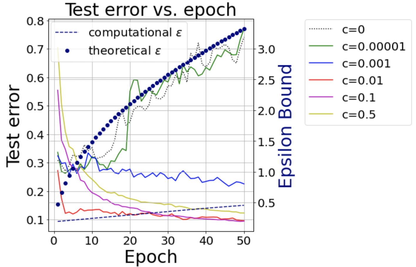
(a) $\sigma=1.6$ for $50$ epochs

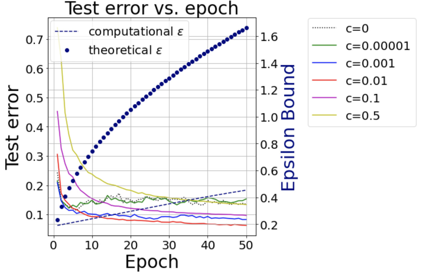
(b) $\sigma=3.2$ for $50$ epochs

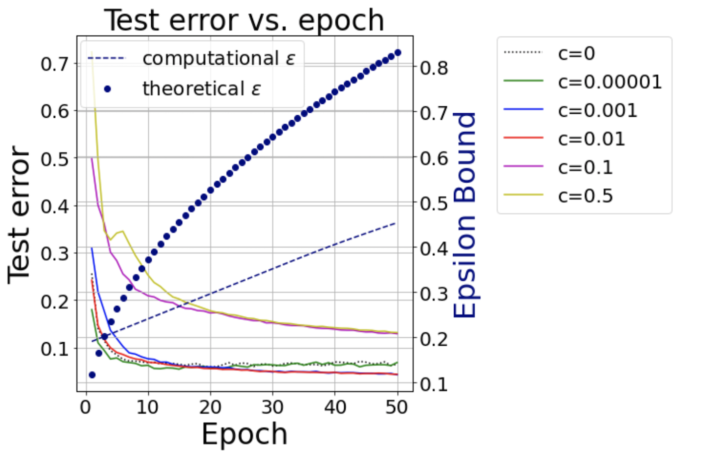
(c) $\sigma=6.4$ for $50$ epochs

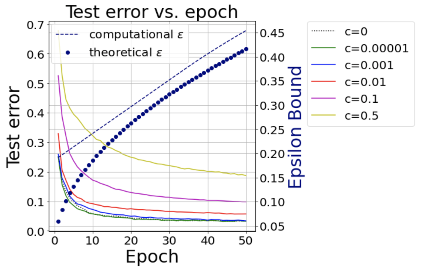
(d) $\sigma=12.8$ for $50$ epochs

Figure 4: Constant stepsize v.s. decaying stepsize for DP-SGD. We plot the test error (not accuracy), corresponding to the left y-axis, with respect to the epoch. Each plot corresponds to a fixed noise $\sigma$. Different color corresponds to a learning rate schedule $\eta_{t}=\eta/b_{t}=1/\sqrt{2+ct}$ with $c$ described in the legend. In addition, we plot the numerical $\varepsilon$ (dash line) and theoretical $\bar{\epsilon}$ (dot plot), corresponding to the right y-axis. We see that the constant learning rate ($c=0$) is not as good as the decaying ones ($c>0$ ).

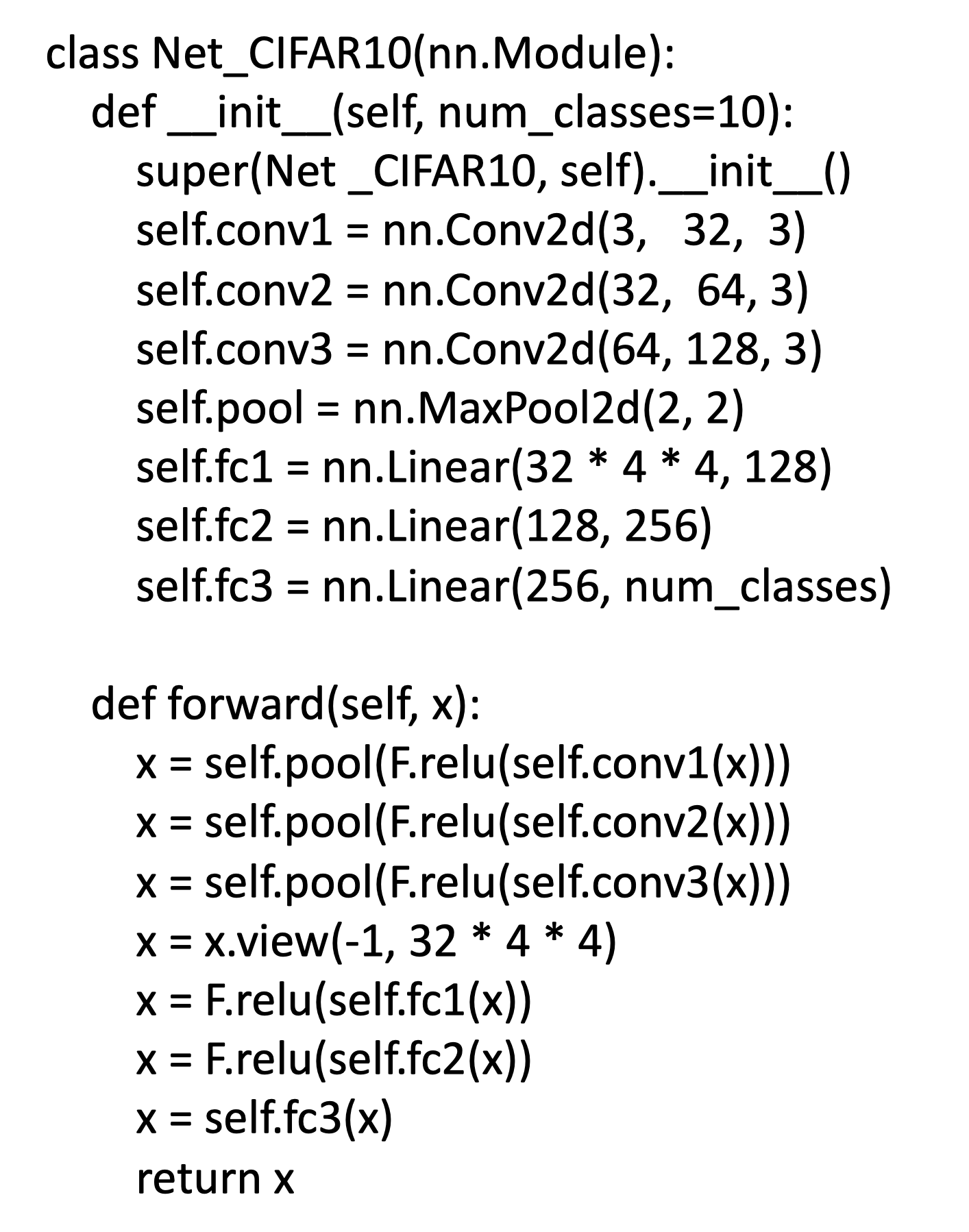
Figure 5: Convolutional Neural Network for CIFAR10.

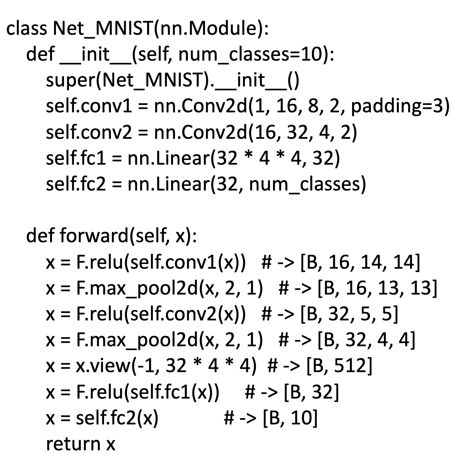
Figure 6: Convolutional Neural Network for MNIST.

F.4 Model architectures

In Figure 5 and 6, we present the CNN models in our experiments written in Python code based on PyTorch.

Appendix G Code Demonstration

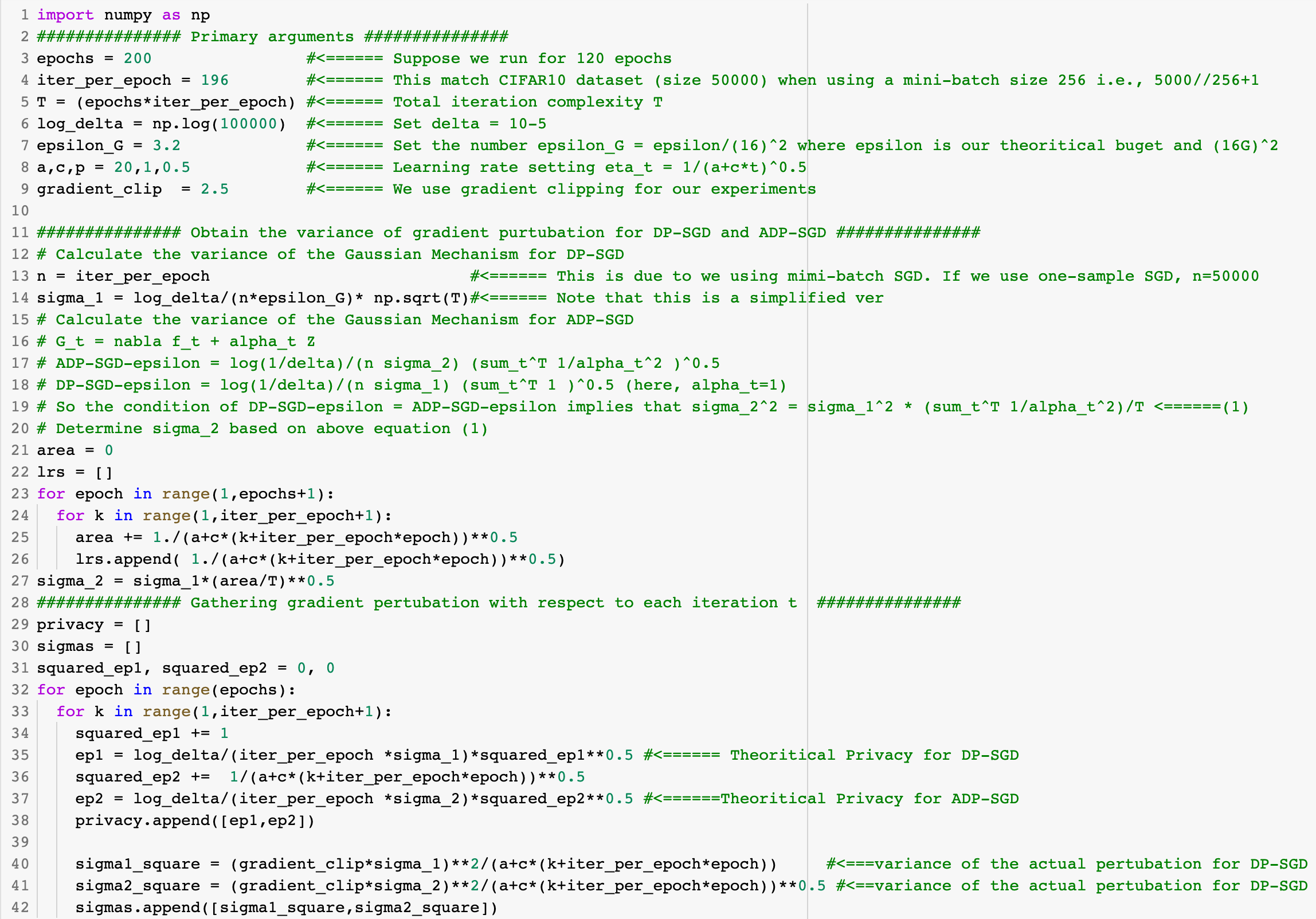
Figure 7: Code to obtain Figure 1

References

- Abadi et al. [2016] M. Abadi, A. Chu, I. Goodfellow, H. B. McMahan, I. Mironov, K. Talwar, and L. Zhang. Deep learning with differential privacy. In Proceedings of the 2016 ACM SIGSAC conference on computer and communications security, pages 308–318, 2016.
- Andrew et al. [2019] G. Andrew, O. Thakkar, H. B. McMahan, and S. Ramaswamy. Differentially private learning with adaptive clipping. arXiv preprint arXiv:1905.03871, 2019.
- Bassily et al. [2014] R. Bassily, A. Smith, and A. Thakurta. Private empirical risk minimization: Efficient algorithms and tight error bounds. In 2014 IEEE 55th Annual Symposium on Foundations of Computer Science, pages 464–473. IEEE, 2014.
- Bassily et al. [2020] R. Bassily, V. Feldman, C. Guzmán, and K. Talwar. Stability of stochastic gradient descent on nonsmooth convex losses. Advances in Neural Information Processing Systems, 33, 2020.
- Bottou et al. [2018] L. Bottou, F. E. Curtis, and J. Nocedal. Optimization methods for large-scale machine learning. SIAM Review, 60(2):223–311, 2018.
- Bu et al. [2020] Z. Bu, J. Dong, Q. Long, and W. J. Su. Deep learning with gaussian differential privacy. Harvard data science review, 2020(23), 2020.
- Carlini et al. [2020] N. Carlini, F. Tramer, E. Wallace, M. Jagielski, A. Herbert-Voss, K. Lee, A. Roberts, T. Brown, D. Song, U. Erlingsson, et al. Extracting training data from large language models. arXiv preprint arXiv:2012.07805, 2020.
- Chaudhuri et al. [2011] K. Chaudhuri, C. Monteleoni, and A. D. Sarwate. Differentially private empirical risk minimization. Journal of Machine Learning Research, 12(3), 2011.
- Chen et al. [2018] X. Chen, S. Liu, R. Sun, and M. Hong. On the convergence of a class of adam-type algorithms for non-convex optimization. In International Conference on Learning Representations, 2018.
- Chen et al. [2020] X. Chen, S. Z. Wu, and M. Hong. Understanding gradient clipping in private sgd: A geometric perspective. Advances in Neural Information Processing Systems, 33, 2020.
- Duchi et al. [2011] J. Duchi, E. Hazan, and Y. Singer. Adaptive subgradient methods for online learning and stochastic optimization. Journal of machine learning research, 12(7), 2011.
- Dwork et al. [2006a] C. Dwork, K. Kenthapadi, F. McSherry, I. Mironov, and M. Naor. Our data, ourselves: Privacy via distributed noise generation. In Annual International Conference on the Theory and Applications of Cryptographic Techniques, pages 486–503. Springer, 2006a.
- Dwork et al. [2006b] C. Dwork, F. McSherry, K. Nissim, and A. Smith. Calibrating noise to sensitivity in private data analysis. In Theory of cryptography conference, pages 265–284. Springer, 2006b.
- Dwork et al. [2010] C. Dwork, G. N. Rothblum, and S. Vadhan. Boosting and differential privacy. In 2010 IEEE 51st Annual Symposium on Foundations of Computer Science, pages 51–60. IEEE, 2010.
- Dwork et al. [2014] C. Dwork, A. Roth, et al. The algorithmic foundations of differential privacy. Foundations and Trends in Theoretical Computer Science, 9(3-4):211–407, 2014.
- Feldman et al. [2020] V. Feldman, T. Koren, and K. Talwar. Private stochastic convex optimization: optimal rates in linear time. In The ACM Symposium on Theory of Computing (STOC), 2020. URL https://dl.acm.org/doi/pdf/10.1145/3357713.3384335.
- Fredrikson et al. [2015] M. Fredrikson, S. Jha, and T. Ristenpart. Model inversion attacks that exploit confidence information and basic countermeasures. In Proceedings of the 22nd ACM SIGSAC Conference on Computer and Communications Security, pages 1322–1333, 2015.
- Ge et al. [2019] R. Ge, S. M. Kakade, R. Kidambi, and P. Netrapalli. The step decay schedule: A near optimal, geometrically decaying learning rate procedure for least squares. In H. Wallach, H. Larochelle, A. Beygelzimer, F. d'Alché-Buc, E. Fox, and R. Garnett, editors, Advances in Neural Information Processing Systems, volume 32. Curran Associates, Inc., 2019. URL https://proceedings.neurips.cc/paper/2019/file/2f4059ce1227f021edc5d9c6f0f17dc1-Paper.pdf.
- Ghadimi and Lan [2013] S. Ghadimi and G. Lan. Stochastic first-and zeroth-order methods for nonconvex stochastic programming. SIAM Journal on Optimization, 23(4):2341–2368, 2013.
- Goyal et al. [2017] P. Goyal, P. Dollár, R. Girshick, P. Noordhuis, L. Wesolowski, A. Kyrola, A. Tulloch, Y. Jia, and K. He. Accurate, large minibatch sgd: Training imagenet in 1 hour. arXiv preprint arXiv:1706.02677, 2017.
- Gupta et al. [2021] U. Gupta, D. Stripelis, P. K. Lam, P. Thompson, J. L. Ambite, and G. V. Steeg. Membership inference attacks on deep regression models for neuroimaging. In Medical Imaging with Deep Learning, 2021. URL https://openreview.net/forum?id=8lL_y9n-CV.
- He et al. [2016] K. He, X. Zhang, S. Ren, and J. Sun. Deep residual learning for image recognition. In Proceedings of the IEEE conference on computer vision and pattern recognition, pages 770–778, 2016.
- Iyengar et al. [2019] R. Iyengar, J. P. Near, D. Song, O. Thakkar, A. Thakurta, and L. Wang. Towards practical differentially private convex optimization. In IEEE Symposium on Security and Privacy, 2019.
- Jayaraman and Wang [2018] B. Jayaraman and L. Wang. Distributed learning without distress: Privacy-preserving empirical risk minimization. Advances in Neural Information Processing Systems, 2018.
- Jayaraman et al. [2020] B. Jayaraman, L. Wang, K. Knipmeyer, Q. Gu, and D. Evans. Revisiting membership inference under realistic assumptions. arXiv preprint arXiv:2005.10881, 2020.
- Jordan and Dimakis [2020] M. Jordan and A. G. Dimakis. Exactly computing the local lipschitz constant of relu networks. In H. Larochelle, M. Ranzato, R. Hadsell, M. F. Balcan, and H. Lin, editors, Advances in Neural Information Processing Systems, volume 33, pages 7344–7353. Curran Associates, Inc., 2020. URL https://proceedings.neurips.cc/paper/2020/file/5227fa9a19dce7ba113f50a405dcaf09-Paper.pdf.
- Kairouz et al. [2017] P. Kairouz, S. Oh, and P. Viswanath. The composition theorem for differential privacy. IEEE Transactions on Information Theory, 63(6):4037–4049, 2017. doi: 10.1109/TIT.2017.2685505.
- Kamath [2020] G. Kamath. Lecture 5: Approximate differential privacy. Lecture Note, 2020. URL http://www.gautamkamath.com/CS860notes/lec5.pdf.
- Kasiviswanathan et al. [2011] S. P. Kasiviswanathan, H. K. Lee, K. Nissim, S. Raskhodnikova, and A. Smith. What can we learn privately? SIAM Journal on Computing, 40(3):793–826, 2011.
- Kifer et al. [2012] D. Kifer, A. Smith, and A. Thakurta. Private convex empirical risk minimization and high-dimensional regression. In Conference on Learning Theory, 2012.
- Kingma and Ba [2014] D. P. Kingma and J. Ba. Adam: A method for stochastic optimization. arXiv preprint arXiv:1412.6980, 2014.
- Koskela and Honkela [2020] A. Koskela and A. Honkela. Learning rate adaptation for differentially private learning. In S. Chiappa and R. Calandra, editors, Proceedings of the Twenty Third International Conference on Artificial Intelligence and Statistics, volume 108 of Proceedings of Machine Learning Research, pages 2465–2475. PMLR, 26–28 Aug 2020.
- Krizhevsky et al. [2009] A. Krizhevsky, G. Hinton, et al. Learning multiple layers of features from tiny images, 2009. https://www.cs.toronto.edu/~kriz/learning-features-2009-TR.pdf.
- Lee and Kifer [2018] J. Lee and D. Kifer. Concentrated differentially private gradient descent with adaptive per-iteration privacy budget. In Proceedings of the 24th ACM SIGKDD International Conference on Knowledge Discovery and Data Mining, pages 1656–1665, 2018.
- Levy et al. [2018] K. Y. Levy, A. Yurtsever, and V. Cevher. Online adaptive methods, universality and acceleration. Advances in Neural Information Processing Systems, 31:6500–6509, 2018.
- Li and Orabona [2019] X. Li and F. Orabona. On the convergence of stochastic gradient descent with adaptive stepsizes. In The 22nd International Conference on Artificial Intelligence and Statistics, pages 983–992. PMLR, 2019.
- McMahan and Streeter [2010] B. McMahan and M. Streeter. Adaptive bound optimization for online convex optimization. Conference on Learning Theory, page 244, 2010.
- Mironov et al. [2019] I. Mironov, K. Talwar, and L. Zhang. Rényi differential privacy of the sampled gaussian mechanism. ArXiv, abs/1908.10530, 2019.
- Nakamura et al. [2020] Y. Nakamura, S. Hanaoka, Y. Nomura, N. Hayashi, O. Abe, S. Yada, S. Wakamiya, and E. Aramaki. Kart: Privacy leakage framework of language models pre-trained with clinical records. arXiv preprint arXiv:2101.00036, 2020.
- Pichapati et al. [2019] V. Pichapati, A. T. Suresh, F. X. Yu, S. J. Reddi, and S. Kumar. Adaclip: Adaptive clipping for private sgd. arXiv preprint arXiv:1908.07643, 2019.
- Reddi et al. [2018] S. J. Reddi, S. Kale, and S. Kumar. On the convergence of adam and beyond. In International Conference on Learning Representations, 2018. URL https://openreview.net/forum?id=ryQu7f-RZ.
- Reddi et al. [2021] S. J. Reddi, Z. Charles, M. Zaheer, Z. Garrett, K. Rush, J. Konecny, S. Kumar, and H. B. McMahan. Adaptive federated optimization. In International Conference on Learning Representations, 2021. URL https://openreview.net/forum?id=LkFG3lB13U5.
- Scaman and Virmaux [2018] K. Scaman and A. Virmaux. Lipschitz regularity of deep neural networks: analysis and efficient estimation. In Proceedings of the 32nd International Conference on Neural Information Processing Systems, pages 3839–3848, 2018.
- Shokri et al. [2017] R. Shokri, M. Stronati, C. Song, and V. Shmatikov. Membership inference attacks against machine learning models. In 2017 IEEE Symposium on Security and Privacy (SP), pages 3–18. IEEE, 2017.
- Song et al. [2013] S. Song, K. Chaudhuri, and A. D. Sarwate. Stochastic gradient descent with differentially private updates. In 2013 IEEE Global Conference on Signal and Information Processing, pages 245–248. IEEE, 2013.
- Vaswani et al. [2017] A. Vaswani, N. Shazeer, N. Parmar, J. Uszkoreit, L. Jones, A. N. Gomez, Ł. Kaiser, and I. Polosukhin. Attention is all you need. In Proceedings of the 31st International Conference on Neural Information Processing Systems, pages 6000–6010, 2017.
- Wang et al. [2020] B. Wang, Q. Gu, M. Boedihardjo, L. Wang, F. Barekat, and S. J. Osher. DP-LSSGD: A stochastic optimization method to lift the utility in privacy-preserving ERM. In J. Lu and R. Ward, editors, Proceedings of The First Mathematical and Scientific Machine Learning Conference, volume 107 of Proceedings of Machine Learning Research, pages 328–351, Princeton University, Princeton, NJ, USA, 20–24 Jul 2020. PMLR.
- Wang et al. [2017] D. Wang, M. Ye, and J. Xu. Differentially private empirical risk minimization revisited: faster and more general. In Proceedings of the 31st International Conference on Neural Information Processing Systems, pages 2719–2728, 2017.
- Wang et al. [2019] L. Wang, B. Jayaraman, D. Evans, and Q. Gu. Efficient privacy-preserving nonconvex optimization. arXiv e-prints, pages arXiv–1910, 2019.
- Ward et al. [2019] R. Ward, X. Wu, and L. Bottou. Adagrad stepsizes: Sharp convergence over nonconvex landscapes. In International Conference on Machine Learning, pages 6677–6686. PMLR, 2019.
- Wu et al. [2017] X. Wu, F. Li, A. Kumar, K. Chaudhuri, S. Jha, and J. Naughton. Bolt-on differential privacy for scalable stochastic gradient descent-based analytics. In ACM International Conference on Management of Data, 2017.
- Zhang et al. [2017] J. Zhang, K. Zheng, W. Mou, and L. Wang. Efficient private ERM for smooth objectives. In International Joint Conference on Artificial Intelligence, 2017.
- Zhou et al. [2020a] Y. Zhou, X. Chen, M. Hong, Z. S. Wu, and A. Banerjee. Private stochastic non-convex optimization: Adaptive algorithms and tighter generalization bounds. arXiv preprint arXiv:2006.13501, 2020a.
- Zhou et al. [2020b] Y. Zhou, B. Karimi, J. Yu, Z. Xu, and P. Li. Towards better generalization of adaptive gradient methods. Advances in Neural Information Processing Systems, 33, 2020b.