Multi-task problems are not multi-objective

Abstract

Multi-objective optimization (MOO) aims at finding a set of optimal configurations for a given set of objectives. A recent line of work applies MOO methods to the typical Machine Learning (ML) setting, which becomes multi-objective if a model should optimize more than one objective, for instance in fair machine learning. These works also use Multi-Task Learning (MTL) problems to benchmark MOO algorithms treating each task as independent objective.

In this work we show that MTL problems do not resemble the characteristics of MOO problems. In particular, MTL losses are not competing in case of a sufficiently expressive single model. As a consequence, a single model can perform just as well as optimizing all objectives with independent models, rendering MOO inapplicable. We provide evidence with extensive experiments on the widely used Multi-Fashion-MNIST datasets. Our results call for new benchmarks to evaluate MOO algorithms for ML. Our code is available at: https://github.com/ruchtem/moo-mtl.

1 Introduction

Multi-Objective Optimization (MOO) is a large field with applications ranging from car design to Adaptive Bitrate Control (Tanabe and Ishibuchi, 2020; Yang et al., 2001; Mao et al., 2017). It is defined as finding the optimal trade-offs between $J$ unweighted objectives:

$$\min_{x\in\mathcal{X}}\left(f_{1}(x),f_{2}(x),\ldots,f_{J}(x)\right)$$ (1)

With recent advances in gradient-based MOO (Fliege and Svaiter, 2000; Désidéri, 2012) an emerging line of deep learning research focuses on applying MOO algorithms for deep neural networks (Sener and Koltun, 2018; Lin et al., 2019a; Navon et al., 2020). These works include casting Multi-Task Learning (MTL) problems into the MOO setting or balancing accuracy and fairness thereby optimizing neural networks for more than one loss. Different to fair machine learning, MTL problems come with the availability of several large-scale datasets and advanced tasks and thus is often used to benchmark MOO approaches (Lin et al., 2019a; Navon et al., 2020; Ruchte and Grabocka, 2021).

In this work we demonstrate that MTL problems differ from MOO problems in a significant way. In particular, the objectives are not necessarily competitive as the network has dedicated parameters for every objective. As a result we can optimize all objectives with just one model (one solution) rather than trading off different objectives which renders MOO inapplicable. In fact, we show that competition is caused by limited model capacity offering the simple solution to just increase the parameters to solve MOO problems.

To confirm our claim we make extensive experiments on the frequently used Multi-MNIST datasets (Lin et al., 2019a).

2 Related work

The foundations for gradient-based MOO were created by (Fliege and Svaiter, 2000) and (Désidéri, 2012). Particularly, Désidéri (2012) derived the Multiple Gradient Descent Algorithm (MGDA) which makes a step towards the minimum norm of the gradients with respect to each objective function, guaranteeing a Pareto-optimal solution. Sener and Koltun (2018) applied this to MTL problems and provided an approximate solution for neural networks which come with a large parameter space. As they demonstrate, applying MOO methods to fit a network for multiple tasks can be a great advantage. This is not to be confused with our claim which questions benchmarking MOO algorithms on MTL problems.

The first work to generate a full Pareto front was Lin et al. (2019a). They proposed to train $k$ models independently, each bound to a region of the objective space, naming their method Pareto Multi-Task Learning (PMTL). The regions are defined by preference rays which reflect a practitioner’s trade-off choices. Two works use hypernetworks (Ha et al., 2016) to condition the parameters on any possible preference ray (Navon et al., 2020; Lin et al., 2020). This way they can approximate the full Pareto front at inference time. We consider Pareto Hypernetworks (PHN) (Navon et al., 2020) as baseline as its code is available. Ruchte and Grabocka (2021) follow a similar idea but condition the model in input feature space by concatenating randomly sampled preference rays to the input features and add a penalty to ensure a well-spread Pareto front.

All methods rely strongly on MTL problems to demonstrate their effectiveness, mainly: Multi-Fashion-MNIST (Lin et al., 2019a), NYUv2 (Nathan Silberman and Fergus, 2012), and CityScapes (Cordts et al., 2016). Navon et al. (2020) and Ruchte and Grabocka (2021) additionally evaluate on fairness problems (e.g. Adult (Kohavi et al., 1996)).

3 Multi-task problems are not multi-objective

In this section we compare the MTL setting with original MOO setting. For MTL the model parameters $\theta$ depend not only on the objective functions $\mathcal{L}$ but also on mini-batches of training data $D$. Thus with a slight change towards common machine learning notation Equation 1 becomes

$$\min_{\theta\in\Theta}\left(\mathcal{L}_{1}(\theta|D),\mathcal{L}_{2}(\theta|D),\ldots,\mathcal{L}_{J}(\theta|D)\right)$$ (2)

This renders MOO a stochastic problem with (generally) non-convex loss functions resulting in approximate solutions with many different local optima. Maybe somewhat more challenging but not fundamentally different to Equation 1. This is the problem to be solved in e.g. fair machine learning where a model should be both accurate but also non-discriminative with respect to some attributes like race or gender. Another example would be recommender systems which should optimize both customer experience and revenue (Lin et al., 2019b).

For MTL, however, each loss is independent of the others as each loss is tied to a specific output of the model. Hence a perfectly valid though naive approach is to optimize a different model for each output (Equation 3).

$$\min_{\theta_{1}\in\Theta_{1},\theta_{2}\in\Theta_{2},\ldots,\theta_{J}\in\Theta_{J}}\left(\mathcal{L}_{1}(\theta_{1}|D),\mathcal{L}_{2}(\theta_{2}|D),\ldots,\mathcal{L}_{J}(\theta_{J}|D)\right)$$ (3)

For efficiency reasons, however, it is common to share some parts of the parameters across tasks (Ruder, 2017):

$$\min_{\theta_{s}\in\Theta_{s},\theta_{1}\in\Theta_{1},\ldots,\theta_{J}\in\Theta_{J}}(\mathcal{L}_{1}(\theta_{s},\theta_{1}|D),\mathcal{L}_{2}(\theta_{s},\theta_{2}|D),\ldots,\mathcal{L}_{J}(\theta_{s},\theta_{J}|D))$$ (4)

where $\theta_{s}$ are shared parameters across all tasks and $\theta_{j}$ are similar to Equation 3 task-specific parameters. This is different to Equation 1 and Equation 2, where there exists no objective-specific part of $x$ or $\theta$. With enough capacity in either $\theta_{s}$ or $\theta_{j}$, the model should be able to optimize all objectives simultaneously as in Equation 3.

4 Experiments

We consider training on a single task (Single Task method) to obtain the optimal score on any given MTL problem (i.e. Equation 3). Additionally, we benchmark six methods: Uniform which minimizes the uniformly weighted sum of all objectives $\min\sum^{J}_{j=1}\frac{1}{J}\mathcal{L}_{j}$; MGDA (Sener and Koltun, 2018); PMTL (Lin et al., 2019a); PHN (linear scalarization if not mentioned otherwise) (Navon et al., 2020); and COSMOS (Ruchte and Grabocka, 2021).

4.1 Experimental setup

We follow the experimental setup of the baselines with fixed 100 training epochs, 256 batch size, and Adam (Kingma and Ba, 2014). As reference point for Hypervolume (HV) (Zitzler et al., 2007) we use $(1,1)$. As model we use LeNet following Lin et al. (2019a). We use the Multi-Fashion-MNIST dataset (Lin et al., 2019a) with predefined splits: 108k training, 12k validation, and 20k test images. In these datasets two instances are merged into one image with a large overlap. The two tasks are to predict the class of each instance. We use the validation images only for HPO and do not merge them for final training. We report final results averaged over ten random seeds. We perform all experiments on Nividia GeForce RTX 2080 GPUs.

Parameter	Range
Learning rate	${1}{\times}10^{-2},{7.5}{\times}10^{-3}$, ${5}{\times}10^{-3},{2.5}{\times}10^{-3}$, $\ldots,{1}{\times}10^{-4}$
Weight decay	${1}{\times}10^{-1},{7.5}{\times}10^{-2}$, ${5}{\times}10^{-2},{2.5}{\times}10^{-2}$, $\ldots,{1}{\times}10^{-4}$
Learning rate scheduler	Cosine Annealing, Step-wise, None

Table 1: Method-independent hyperparameter search spaces

Hyperparameter optimization.

We perform random search over the hyperparameter search spaces defined in Table 1. Learning rate scheduler specifics are ${1}{\times}10^{-6}$ as minimum learning rate for Cosine Annealing (Loshchilov and Hutter, 2016) and Step-wise with milestones at epoch 33 and 66 with multiplier 0.1. We sample 100 configurations uniformly at random, which covers approximately 30% of the $9\times 13\times 3=351$ possible combinations. We select the best configuration based on Hypervolume based on cross-entropy loss measured on the validation set.

Some methods come with their own set of hyperparameters. For MGDA this is gradient normalization $\in\{\text{l2},\text{loss},\text{loss+},\text{None}\}$. For PHN this is the internal solver $\in\{\text{ls},\text{EPO}\}$ and the Dirichlet sampling parameter $\alpha\in\{0.1,0.2,0.5,1,1.2,1.5\}$. For COSMOS this is $\alpha$ and the cosine penalty weight $\lambda\in\{1,2,4,8,16\}$. The ranges are chosen to cover the original values plus one value beyond. Method-specific HPO covers a smaller part of the search space, approximately 7, 2.37, and 0.95 Percent for MGDA, PHN, and COSMOS, respectively. We denote these methods with an asterix (^∗). For PHN and COSMOS we provide also results not optimizing the internal solver, $\alpha$, or $\lambda$ taking the original values reported by the authors. See Section A in the supplementary for the parameters found by HPO.

4.2 Results

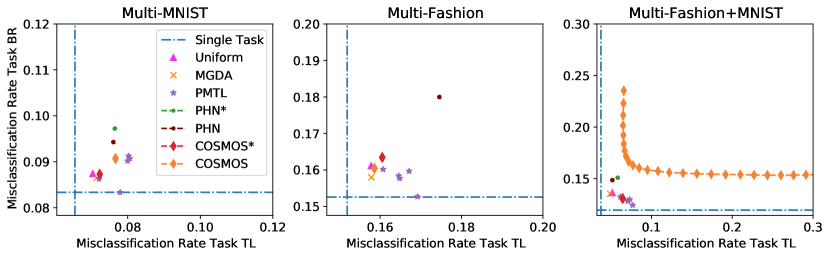
Figure 1: Results on Multi-MNIST dataset for different methods. Linear scalarization with uniform weights (Uniform) is a competetive baseline despite its simplicity given its hyperparameters are properly tuned.

Method	Params	Multi MNIST		Multi Fashion		multi fashion+mnist
		HV $\uparrow$	$\Delta$ ST $\downarrow$	HV $\uparrow$	$\Delta$ ST $\downarrow$	HV $\uparrow$	$\Delta$ ST $\downarrow$
PMTL	211k	0.8509 $\pm$ 0.0023	0.0058	0.7139 $\pm$ 0.0056	0.0048	0.8220 $\pm$ 0.0062	0.0254
PHN∗	3,243k	0.8337 $\pm$ 0.0041	0.0229	0.6769 $\pm$ 0.0143	0.0417	0.7996 $\pm$ 0.0053	0.0478
PHN		0.8368 $\pm$ 0.0046	0.0198	0.6769 $\pm$ 0.0143	0.0417	0.8073 $\pm$ 0.0051	0.0401
COSMOS∗	42k	0.8467 $\pm$ 0.0039	0.0099	0.7023 $\pm$ 0.0087	0.0164	0.8132 $\pm$ 0.0026	0.0342
COSMOS		0.8396 $\pm$ 0.0047	0.0170	0.7064 $\pm$ 0.0055	0.0123	0.7915 $\pm$ 0.0111	0.0559
MGDA∗	42k	0.8482 $\pm$ 0.0060	0.0084	0.7091 $\pm$ 0.0040	0.0096	0.8222 $\pm$ 0.0046	0.0252
Uniform	42k	0.8484 $\pm$ 0.0091	0.0083	0.7065 $\pm$ 0.0111	0.0121	0.8189 $\pm$ 0.0067	0.0285
Single Task	42k	0.8566 $\pm$ 0.0023	-	0.7187 $\pm$ 0.0036	-	0.8474 $\pm$ 0.0028	-

Table 2: Hypervolume (HV) based on misclassification rates of properly optimized methods for the Multi-Mnist datasets (larger is better). $\Delta$ ST denotes the distance of each method to Single Task, an indication whether the problem is multi-objective. ^∗ denotes optimizing method-specific hyperparameters as well. Italic denotes the second-best method after Single Task. Linear scalarization with uniform weights (Uniform) is a competetive baseline despite its simplicity given its hyperparameters are properly tuned. Surprisingly, almost all Pareto front generating models (upper section) are not competitive even though their hyperparameters are also tuned to maximize HV.

We show the results in terms of Misclassification Rate (MCR) in Figure 1 and Table 2. We can see that Uniform despite being by far the most simple method is competitive compared to the more complex methods and achieves nearly the same performance as Single Task. The gap between Uniform and Single Task is larger for Multi-Fashion indicating that here the two tasks are indeed competing. We hypothesis, however, this is due to the limited capacity of the model and results with different model size in Section 4.3. For scores on each task and cross-entropy results see Section B in the supplementary.

Unsurprisingly, using HPO improves performance of all methods when comparing to the numbers reported by the authors. For instance, PMTL reports Single Task MCR on Multi-MNIST Top-Left of 0.91 and Bottom-Right of 0.88, whereas we get 0.93 and 0.91, respectively. Same is true for the other datasets and methods. This underlines the importance of HPO for proper method evaluation. Particularly, surpassing Single Task models in MTL settings should raise concerns regarding overfitting and thus unfair comparisons.

Somewhat surprising is that even methods which can generate a Pareto front (especially PHN and COSMOS), do not produce one when their learning rate, weight decay and scheduler are optimized for validation HV. This problem was already mentioned by Ruchte and Grabocka (2021) and their main motivation to introduce the cosine penalty. We double checked and there were HPO configurations sampled which resulted in a Pareto front but actually achieved a much lower HV score. We see this as a further indication that we are not looking at an MOO problem.

4.3 Ablations

Dataset	Single Task HV	Uniform HV
MM	0.8551 $\pm$ 0.0033	0.8488 $\pm$ 0.0056
MF	0.7234 $\pm$ 0.0028	0.7122 $\pm$ 0.0075
MFM	0.8442 $\pm$ 0.0034	0.8200 $\pm$ 0.0068

Table 3: Grid seach HV results.

Grid search.

To quantify a possible negative impact of random search in HPO we also perform grid search over all possible 351 hyperparameter combinations and report the results for a subset of the methods in Table 3. Datasets are abbreviated as MM (Multi-MNIST), MF (Multi-Fashion), and MFM (Multi-Fashion-MNIST). There are almost no significant differences when comparing to Table 2 which demonstrates that randomly searching about one third of the search space is a valid approach in our case.

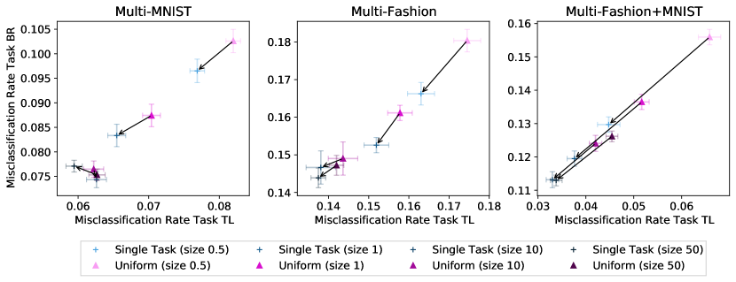
Figure 2: Results for Single Task and Uniform when varying the capacity of the model. Errorbars denote standard deviation. We can see that the distance between Single Task and Uniform (black arrows) as well as the absolute error decrease significantly when increasing the capacity of the model.

Model capacity.

We ask the question whether capacity plays a crucial role in rendering MTL problems multi-objective with tasks competing against each other. For this we alter the capacity of the model by changing the number of channels with a multiplier. Specifically, we change the model to have $10c$ channels in the first layer and $20c$ channels in the second layer where $c\in\{0.5,1,10,50\}$ is the channel multiplier (i.e. we only alter $\theta_{s}$).

The results are presented in Figure 2 and Table 4. We can see that the distance between Single Task and Uniform scores indeed depends on the capacity of the models. Reducing capacity increases the distance, increasing capacity decreases the distance up to a saturation point where error rates almost match. Interestingly, for Multi-Fashion-MNIST there is still a considerable gap between single task and uniform performance. This could be an indication that not only capacity matters but also the similarity of the tasks.

The experiments support the hypothesis that for MTL problems it is more beneficial to increase the capacity instead of treating it as a MOO problem trying to balance presumed conflicts between losses. This is especially true for methods which inherently increase the capacity as PHN does. Multiplying the channels by 10 and using uniform scalarization yields a better Hypervolume with about 25% of the parameters compared to PHN (0.03 HV improve on Multi-MNIST).

Method	$c$	Params	Multi Mnist		Multi fashion		Multi fashion+mnist
			HV	$\Delta$ ST	HV	$\Delta$ ST	HV	$\Delta$ ST
Single Task	0.5x	20k	0.8340 $\pm$ 0.0028	-	0.6978 $\pm$ 0.0045	-	0.8313 $\pm$ 0.0025	-
Uniform			0.8238 $\pm$ 0.0065	0.0102	0.6767 $\pm$ 0.0143	0.0212	0.7885 $\pm$ 0.0095	0.0428
Single Task	1x	42k	0.8566 $\pm$ 0.0023	-	0.7187 $\pm$ 0.0036	-	0.8474 $\pm$ 0.0028	-
Uniform			0.8484 $\pm$ 0.0091	0.0083	0.7065 $\pm$ 0.0111	0.0121	0.8189 $\pm$ 0.0067	0.0285
Single Task	10x	863k	0.8677 $\pm$ 0.0022	-	0.7355 $\pm$ 0.0042	-	0.8576 $\pm$ 0.0025	-
Uniform			0.8661 $\pm$ 0.0023	0.0016	0.7288 $\pm$ 0.0107	0.0067	0.8391 $\pm$ 0.0026	0.0184
Single Task	50x	14,315k	0.8680 $\pm$ 0.0012	-	0.7384 $\pm$ 0.0033	-	0.8571 $\pm$ 0.0023	-
Uniform			0.8667 $\pm$ 0.0032	0.0013	0.7317 $\pm$ 0.0076	0.0067	0.8341 $\pm$ 0.0042	0.0230

Table 4: Ablation results for different model sizes. $c$ denotes the channel multiplier, $\Delta$ ST denotes the distance of each method to Single Task. The results show that $\Delta$ ST decreases on overall when increasing the model capacity.

5 Limitations

One limitation is that we did not do proper HPO for methods with additional hyperparameters as this would result in unbearable computing costs. For the same reason we also used only one seed for HPO, despite the results in Section 4.3 being aware that the obtained scores are noisy.

Also due to computing costs we decided to not repeat the analysis with larger models on one of the larger benchmarks mentioned in Section 2. We, however, do not see a reason why the results should not generalize to larger problems. This could be a direction for future research, as well as an analysis on the effect of altering the capacity of the task-specific heads, i.e. $\theta_{j}$.

6 Conclusion

In this work we showed that multi-task problems do not necessarily resemble the characteristics of multi-objective problems. One important aspect in rendering MTL tasks multi-objective is the capacity of the model and likely the similarity between the tasks. The results call for a new set of benchmarks which are truly multi-objective. Pointers could be Fairness (Navon et al., 2020; Ruchte and Grabocka, 2021) and recommender systems (Lin et al., 2019b; Milojkovic et al., 2019). Especially the latter come with large datasets and require large models which is more suited for deep neural networks. Another pointer is Deist et al. (2021) who evaluate on medical image segmentation with possibly conflicting labeling.

It required roughly 3100 GPU hours to compute the results presented here, where 2780 are due to the ablations.

Appendix

Appendix A HPO results

We show the hyperparameter values found by hyperparameter optimization for Section 4.2 in Table 5 and for Section 4.3 in Table 6.

Parameter	Dataset	ST TL	ST BR	Uniform	MGDA	PMTL	PHN	PHN∗	COSMOS	COSMOS∗
Lerning rate	MM	0.0005	0.00075	0.0025	0.001	0.00025	0.00075	0.001	0.00075	0.001
	MF	0.0025	0.001	0.00075	0.0025	0.00075	0.00075	0.00075	0.001	0.00075
	MFM	0.0025	0.00075	0.00075	0.001	0.00075	0.0005	0.0025	0.0075	0.001
Weight decay	MM	0.05	0.05	0.0075	0.01	0.075	0.05	0.075	0.0075	0.0075
	MF	0.01	0.01	0.01	0.005	0.05	0.075	0.075	0.0075	0.0075
	MFM	0.0075	0.01	0.01	0.01	0.05	0.075	0.005	0.0005	0.01
Learning rate scheduler	MM	CA	MS	CA	CA	CA	CA	CA	CA	CA
	MF	MS	CA	CA	CA	CA	CA	CA	CA	CA
	MFM	CA	MS	CA	CA	CA	CA	CA	CA	MS
Normal- ization	MM	-	-	-	loss	-	-	-	-	-
	MF	-	-	-	loss+	-	-	-	-	-
	MFM	-	-	-	none	-	-	-	-	-
Internal solver	MM	-	-	-	-	-	linear†	epo	-	-
	MF	-	-	-	-	-	linear†	linear	-	-
	MFM	-	-	-	-	-	linear†	linear	-	-
$\alpha$	MM	-	-	-	-	-	0.2†	0.1	1.2†	0.5
	MF	-	-	-	-	-	0.2†	0.2	1.2†	1.0
	MFM	-	-	-	-	-	0.2†	1.2	1.2†	0.2
$\lambda$	MM	-	-	-	-	-	-	-	2†	1
	MF	-	-	-	-	-	-	-	2†	2
	MFM	-	-	-	-	-	-	-	8†	1

Table 5: Hyperparameters found by HPO, ^†denotes the values from the original works, here just for reference. MM=Multi MNIST, MF=Multi Fashion, MFM=Multi Fashion+MNIST.

Parameter	Dataset	Single Task TL			Single Task BR			Uniform
		0.5x	10x	50x	0.5x	10x	50x	0.5x	10x	50x
Lerning rate	MM	0.001	0.0001	0.0001	0.00075	0.00025	0.00025	0.0005	0.0005	0.0001
	MF	0.001	0.00075	0.0005	0.0025	0.001	0.0005	0.0025	0.00075	0.0005
	MFM	0.001	0.0005	0.00075	0.0025	0.00075	0.00025	0.0025	0.0005	0.0005
Weight decay	MM	0.05	0.01	0.01	0.01	0.01	0.01	0.0075	0.0075	0.0075
	MF	0.0075	0.01	0.01	0.005	0.0075	0.01	0.005	0.0075	0.0075
	MFM	0.01	0.01	0.01	0.0075	0.01	0.01	0.0075	0.0075	0.005
Learning rate scheduler	MM	MS	MS	MS	MS	MS	CA	CA	MS	MS
	MF	MS	MS	MS	MS	CA	CA	CA	CA	MS
	MFM	MS	MS	CA	MS	MA	MS	CA	MS	CA

Table 6: Hyperparameters found by HPO for the models with different capacity. The second row in the header refers to the channel multiplier (see Section 4.3). MM=Multi MNIST, MF=Multi Fashion, MFM=Multi Fashion+MNIST. Learning rate scheduler abbreviations: MS=Step-wise (multi step), CA=Cosine Annealing.

Appendix B More results

We show the performance in terms of Misclassification rate for each task in Table 7. The performance for each task in terms of cross entropy is shown in Figure 3 and Table 9. An equivalent of Table 2 for Hypervolume calculated based on cross entropy is presented in Table 8.

Method	Multi MNIST		Multi Fashion		multi fashion+mnist
	TL	BR	TL	BR	TL	BR
Single Task	0.0655 $\pm$ 0.0013	0.0834 $\pm$ 0.0023	0.1519 $\pm$ 0.0031	0.1526 $\pm$ 0.0020	0.0376 $\pm$ 0.0015	0.1195 $\pm$ 0.0023
Uniform	0.0704 $\pm$ 0.0051	0.0874 $\pm$ 0.0051	0.1578 $\pm$ 0.0070	0.1611 $\pm$ 0.0066	0.0517 $\pm$ 0.0041	0.1365 $\pm$ 0.0036
MGDA	0.0715 $\pm$ 0.0032	0.0865 $\pm$ 0.0036	0.1579 $\pm$ 0.0038	0.1580 $\pm$ 0.0030	0.0490 $\pm$ 0.0029	0.1354 $\pm$ 0.0035
ParetoMTL	0.0806 $\pm$ 0.0030	0.0907 $\pm$ 0.0023	0.1646 $\pm$ 0.0064	0.1584 $\pm$ 0.0047	0.0732 $\pm$ 0.0044	0.1298 $\pm$ 0.0030
PHN∗	0.0765 $\pm$ 0.0020	0.0972 $\pm$ 0.0031	0.1746 $\pm$ 0.0092	0.1800 $\pm$ 0.0085	0.0583 $\pm$ 0.0038	0.1509 $\pm$ 0.0036
PHN	0.0761 $\pm$ 0.0025	0.0943 $\pm$ 0.0031	0.1746 $\pm$ 0.0092	0.1800 $\pm$ 0.0085	0.0518 $\pm$ 0.0041	0.1486 $\pm$ 0.0030
COSMOS∗	0.0723 $\pm$ 0.0022	0.0873 $\pm$ 0.0025	0.1605 $\pm$ 0.0051	0.1634 $\pm$ 0.0058	0.0645 $\pm$ 0.0012	0.1308 $\pm$ 0.0023
COSMOS	0.0767 $\pm$ 0.0028	0.0907 $\pm$ 0.0029	0.1586 $\pm$ 0.0026	0.1604 $\pm$ 0.0047	0.1081 $\pm$ 0.0069	0.1573 $\pm$ 0.0061

Table 7: Results for each task in terms of Misclassification rate (MRC)

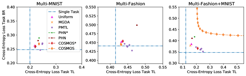
Figure 3: Results in terms of cross-entropy loss

Method	Multi MNIST		Multi Fashion		multi fashion+mnist
	HV	$\Delta$ ST	HV	$\Delta$ ST	HV	$\Delta$ ST
Single Task	0.6024 $\pm$ 0.0048	0	0.3272 $\pm$ 0.0043	0	0.5732 $\pm$ 0.0072	0
Uniform	0.5777 $\pm$ 0.0191	0.0248	0.3116 $\pm$ 0.0202	0.0157	0.5147 $\pm$ 0.0148	0.0584
MGDA∗	0.5789 $\pm$ 0.0158	0.0235	0.3168 $\pm$ 0.0072	0.0104	0.5254 $\pm$ 0.0102	0.0478
PMTL	0.5888 $\pm$ 0.0080	0.0136	0.3261 $\pm$ 0.0106	0.0011	0.5209 $\pm$ 0.0160	0.0523
PHN∗	0.5438 $\pm$ 0.0097	0.0586	0.2631 $\pm$ 0.0247	0.0641	0.4738 $\pm$ 0.0119	0.0994
PHN	0.5539 $\pm$ 0.0110	0.0485	0.2631 $\pm$ 0.0247	0.0641	0.4905 $\pm$ 0.0099	0.0827
COSMOS∗	0.5772 $\pm$ 0.0102	0.0252	0.3082 $\pm$ 0.0172	0.0190	0.5011 $\pm$ 0.0069	0.0720
COSMOS	0.5603 $\pm$ 0.0106	0.0421	0.3159 $\pm$ 0.0118	0.0113	0.4563 $\pm$ 0.0219	0.1169

Table 8: Hypervolume (HV) results based on cross-entropy loss

Method	Multi MNIST		Multi Fashion		multi fashion+mnist
	TL	BR	TL	BR	TL	BR
Single Task	0.1993 $\pm$ 0.0035	0.2476 $\pm$ 0.0055	0.4151 $\pm$ 0.0059	0.4405 $\pm$ 0.0047	0.1219 $\pm$ 0.0050	0.3473 $\pm$ 0.0067
Uniform	0.2174 $\pm$ 0.0139	0.2621 $\pm$ 0.0123	0.4318 $\pm$ 0.0190	0.4523 $\pm$ 0.0186	0.1634 $\pm$ 0.0122	0.3849 $\pm$ 0.0093
MGDA	0.2189 $\pm$ 0.0105	0.2589 $\pm$ 0.0114	0.4316 $\pm$ 0.0079	0.4426 $\pm$ 0.0071	0.1558 $\pm$ 0.0070	0.3776 $\pm$ 0.0087
ParetoMTL	0.2476 $\pm$ 0.0091	0.2706 $\pm$ 0.0062	0.4489 $\pm$ 0.0190	0.4380 $\pm$ 0.0155	0.2375 $\pm$ 0.0127	0.3644 $\pm$ 0.0066
PHN∗	0.2347 $\pm$ 0.0056	0.2895 $\pm$ 0.0079	0.4761 $\pm$ 0.0273	0.4989 $\pm$ 0.0239	0.1871 $\pm$ 0.0106	0.4172 $\pm$ 0.0104
PHN	0.2308 $\pm$ 0.0074	0.2799 $\pm$ 0.0084	0.4761 $\pm$ 0.0273	0.4989 $\pm$ 0.0239	0.1681 $\pm$ 0.0102	0.4105 $\pm$ 0.0075
COSMOS∗	0.2208 $\pm$ 0.0065	0.2592 $\pm$ 0.0076	0.4360 $\pm$ 0.0144	0.4540 $\pm$ 0.0176	0.2101 $\pm$ 0.0040	0.3656 $\pm$ 0.0063
COSMOS	0.2342 $\pm$ 0.0073	0.2684 $\pm$ 0.0080	0.4306 $\pm$ 0.0096	0.4453 $\pm$ 0.0127	0.3504 $\pm$ 0.0160	0.4289 $\pm$ 0.0124

Table 9: Results for each task in terms of cross-entropy loss

References

- Cordts et al. [2016] Marius Cordts, Mohamed Omran, Sebastian Ramos, Timo Rehfeld, Markus Enzweiler, Rodrigo Benenson, Uwe Franke, Stefan Roth, and Bernt Schiele. The cityscapes dataset for semantic urban scene understanding. In Proc. of the IEEE Conference on Computer Vision and Pattern Recognition (CVPR), 2016.
- Deist et al. [2021] Timo M Deist, Monika Grewal, Frank JWM Dankers, Tanja Alderliesten, and Peter AN Bosman. Multi-objective learning to predict pareto fronts using hypervolume maximization. arXiv preprint arXiv:2102.04523, 2021.
- Désidéri [2012] Jean-Antoine Désidéri. Mutiple-gradient descent algorithm for multiobjective optimization. In European Congress on Computational Methods in Applied Sciences and Engineering (ECCOMAS 2012), 2012.
- Fliege and Svaiter [2000] Jörg Fliege and Benar Fux Svaiter. Steepest descent methods for multicriteria optimization. Mathematical methods of operations research, 51(3):479–494, 2000.
- Ha et al. [2016] David Ha, Andrew Dai, and Quoc V Le. Hypernetworks. arXiv preprint arXiv:1609.09106, 2016.
- Kingma and Ba [2014] Diederik P Kingma and Jimmy Ba. Adam: A method for stochastic optimization. arXiv preprint arXiv:1412.6980, 2014.
- Kohavi et al. [1996] Ron Kohavi et al. Scaling up the accuracy of naive-bayes classifiers: A decision-tree hybrid. In Kdd, volume 96, pages 202–207, 1996.
- Lin et al. [2019a] Xi Lin, Hui-Ling Zhen, Zhenhua Li, Qing-Fu Zhang, and Sam Kwong. Pareto multi-task learning. Advances in neural information processing systems, 32:12060–12070, 2019a.
- Lin et al. [2020] Xi Lin, Zhiyuan Yang, Qingfu Zhang, and Sam Kwong. Controllable pareto multi-task learning. arXiv preprint arXiv:2010.06313, 2020.
- Lin et al. [2019b] Xiao Lin, Hongjie Chen, Changhua Pei, Fei Sun, Xuanji Xiao, Hanxiao Sun, Yongfeng Zhang, Wenwu Ou, and Peng Jiang. A pareto-efficient algorithm for multiple objective optimization in e-commerce recommendation. In Proceedings of the 13th ACM Conference on recommender systems, pages 20–28, 2019b.
- Loshchilov and Hutter [2016] Ilya Loshchilov and Frank Hutter. Sgdr: Stochastic gradient descent with warm restarts. arXiv preprint arXiv:1608.03983, 2016.
- Mao et al. [2017] Hongzi Mao, Ravi Netravali, and Mohammad Alizadeh. Neural adaptive video streaming with pensieve. In Proceedings of the Conference of the ACM Special Interest Group on Data Communication, pages 197–210, 2017.
- Milojkovic et al. [2019] Nikola Milojkovic, Diego Antognini, Giancarlo Bergamin, Boi Faltings, and Claudiu Musat. Multi-gradient descent for multi-objective recommender systems. arXiv preprint arXiv:2001.00846, 2019.
- Nathan Silberman and Fergus [2012] Pushmeet Kohli Nathan Silberman, Derek Hoiem and Rob Fergus. Indoor segmentation and support inference from rgbd images. In ECCV, 2012.
- Navon et al. [2020] Aviv Navon, Aviv Shamsian, Ethan Fetaya, and Gal Chechik. Learning the pareto front with hypernetworks. In International Conference on Learning Representations, 2020.
- Ruchte and Grabocka [2021] Michael Ruchte and Josif Grabocka. Scalable pareto front approximation for deep multi-objective learning. Proceedings of the IEEE International Conference on Data Mining (ICDM), 2021.
- Ruder [2017] Sebastian Ruder. An overview of multi-task learning in deep neural networks. arXiv preprint arXiv:1706.05098, 2017.
- Sener and Koltun [2018] Ozan Sener and Vladlen Koltun. Multi-task learning as multi-objective optimization. In Proceedings of the 32nd International Conference on Neural Information Processing Systems, pages 525–536, 2018.
- Tanabe and Ishibuchi [2020] Ryoji Tanabe and Hisao Ishibuchi. An easy-to-use real-world multi-objective optimization problem suite. Applied Soft Computing, 89:106078, 2020.
- Yang et al. [2001] RJ Yang, N Wang, CH Tho, JP Bobineau, and BP Wang. Metamodeling development for vehicle frontal impact simulation. In International Design Engineering Technical Conferences and Computers and Information in Engineering Conference, volume 80227, pages 27–35. American Society of Mechanical Engineers, 2001.
- Zitzler et al. [2007] Eckart Zitzler, Dimo Brockhoff, and Lothar Thiele. The hypervolume indicator revisited: On the design of pareto-compliant indicators via weighted integration. In International Conference on Evolutionary Multi-Criterion Optimization, pages 862–876. Springer, 2007.