[table]capposition=top
Carousel Memory: Rethinking the Design of Episodic Memory for Continual Learning
Abstract
Continual Learning (CL) is an emerging machine learning paradigm that aims to learn from a continuous stream of tasks without forgetting knowledge learned from the previous tasks. To avoid performance decrease caused by forgetting, prior studies exploit episodic memory (EM), which stores a subset of the past observed samples while learning from new non-i.i.d. data. Despite the promising results, since CL is often assumed to execute on mobile or IoT devices, the EM size is bounded by the small hardware memory capacity and makes it infeasible to meet the accuracy requirements for real-world applications. Specifically, all prior CL methods discard samples overflowed from the EM and can never retrieve them back for subsequent training steps, incurring loss of information that would exacerbate catastrophic forgetting. We explore a novel hierarchical EM management strategy to address the forgetting issue. In particular, in mobile and IoT devices, real-time data can be stored not just in high-speed RAMs but in internal storage devices as well, which offer significantly larger capacity than the RAMs. Based on this insight, we propose to exploit the abundant storage to preserve past experiences and alleviate the forgetting by allowing CL to efficiently migrate samples between memory and storage without being interfered by the slow access speed of the storage. We call it Carousel Memory (CarM). As CarM is complementary to existing CL methods, we conduct extensive evaluations of our method with seven popular CL methods and show that CarM significantly improves the accuracy of the methods across different settings by large margins in final average accuracy (up to 28.4%) while retaining the same training efficiency.
1 Introduction
With the rising demand for realistic on-device machine learning, recent years have witnessed a novel learning paradigm, namely continual learning (CL), for training neural networks (NN) with a stream of non-i.i.d. data. In such a paradigm, the neural network is incrementally learned with insertions of new tasks (e.g., a set of classes) (Rebuffi et al., 2017). The NN model is expected to continuously learn new knowledge from new tasks over time while retaining previously learned knowledge, which is a closer representation of how intelligent systems operate in the real world. In this learning setup, the knowledge should be acquired not only from the new data timely but also in a computationally efficient manner. In this regard, CL is suitable for learning on mobile and IoT devices (Hayes et al., 2020; Wang et al., 2019).
However, CL faces significant challenges from the notorious catastrophic forgetting problem—knowledge learned in the past fading away as the NN model continues to learn new tasks (McCloskey & Neal, 1989). Among many prior approaches to addressing this issue, episodic memory (EM) is one of the most effective approaches (Buzzega et al., 2020; Chaudhry et al., 2019a; b; Lopez-Paz & Ranzato, 2017; Prabhu et al., 2020). EM is an in-memory buffer that stores old samples and replays them periodically while training models with new samples. EM needs to have a sufficiently large capacity to achieve a desired accuracy, and such capacity in need may vary significantly since incoming data may contain a varying number of tasks and classes at different time slots and geo-locations (Bang et al., 2021). However, in practice, the size of EM is often quite small, bounded by limited on-device memory capacity. The limited EM size makes it difficult to store a large number of samples or scale up to a large number of tasks, preventing CL models from achieving high accuracy as training moves forward. To address the forgetting problem, we introduce a hierarchical EM method, which significantly enhances the effectiveness of episodic memory. Our method is motivated by the fact that modern mobile and IoT devices are commonly equipped with a deep memory hierarchy including small memory with fast access (50–150 ns) and large storage with slow access (25–250 s), which is typically orders of magnitude larger than the memory. Provided by these different hardware characteristics, the memory is an ideal place to access samples at high speed during training, promising short training time. In contrast, the storage is an ideal place to store a significantly large number of old samples and use them for greatly improving model accuracy. The design goal of our scheme, Carousel Memory or CarM, is to combine the best of both worlds to improve the episodic memory capacity by leveraging on-device storage but without significantly prolonging traditional memory-based CL approaches.
CarM stores as many observed samples as possible so long as it does not exceed a given storage capacity (rather than discarding those overflowed from EM as done in existing methods) and updates the in-memory EM while the model is still learning with samples already in EM. One key research question is how to manage samples across EM and storage for both system efficiency and model accuracy. Here we propose a hierarchical memory-aware data swapping, an online process that dynamically replaces a subset of in-memory samples used for model training with other samples stored in storage, with an optimization goal in two aspects. (1) System efficiency. Prior single-level memory-only training approaches promise timely model updates even in the face of real-time data that arrives with high throughput. Therefore, we expect drawing old samples from slow storage does not incur significant I/O overhead that affects the overall system efficiency, especially for mobile and IoT devices. (2) Model accuracy. CarM significantly increases the effective EM size, mitigating forgetting issues by avoiding important information from overflowing due to limited memory capacity. As a result, we expect our approach also improves the model accuracy by exploiting data samples preserved in the storage more effectively for training. To fulfill the competing goals, we design CarM from two different perspectives: swapping mechanism (Section 3.1) and swapping policy (Section 3.2). The swapping mechanism of CarM ensures that the slow speed of accessing the storage does not become a bottleneck of continual model training by carefully hiding sample swapping latency through asynchrony. Moreover, we propose various swapping policies to decide which and when to swap samples and incorporate them into a single component, namely, gate function. The gate function allows for fewer swapping samples, making CarM to march with low I/O bandwidth storage which is common for mobile and IoT devices.
One major benefit of CarM is that it is largely complementary to existing episodic memory-based CL methods. By exploiting the memory hierarchy, we show that CarM helps boost the accuracy of many existing methods by up to 28.4% for DER++ (Buzzega et al., 2020) in Tiny-ImageNet dataset (Section 4.1) and even allows them to retain their accuracy with much smaller EM sizes.
With CarM as a strong baseline for episodic memory-based CL methods, some well-known algorithmic optimizations may need to be revisited to ensure that they are not actually at odds with data swapping. For example, we observe that iCaRL (Rebuffi et al., 2017), BiC (Wu et al., 2019), and DER++ (Buzzega et al., 2020), which strongly depend on knowledge distillation for old tasks, can deliver higher accuracy with CarM by limiting the weight coefficient on the distillation loss as a small value in calculating training loss. With CarM, such weight coefficient does not indeed necessarily be high or managed complicatedly as done in prior work, because we could now leverage a large amount of data in storage (with ground truth) to facilitate training performance.
2 Related Work
Class incremental learning. The performance of CL algorithms heavily depends on scenarios and setups, as summarized by Van de Ven et al. (van de Ven & Tolias, 2018). Among them, we are particularly interested in class-incremental learning (CIL), where task IDs are not given during inference (Gepperth & Hammer, 2016). Many prior proposals are broadly divided into two categories, rehearsal-based and regularization-based. In rehearsal-based approaches, episodic memory stores a few samples of old tasks to replay in the future (Bang et al., 2021; Castro et al., 2018; Chaudhry et al., 2018; Rebuffi et al., 2017). On the contrary, regularization-based approaches exploit the information of old tasks implicitly retained in the model parameters, without storing samples representing old tasks (Kirkpatrick et al., 2017; Zenke et al., 2017; Liu et al., 2018; Li & Hoiem, 2017; Lee et al., 2017; Mallya et al., 2018). As rehearsal-based approaches generally have shown the better performance in CIL (Prabhu et al., 2020), we aim to alleviate current drawbacks of the approaches (i.e., limited memory space) by incorporating data management across the memory-storage hierarchy.
The CIL setup usually assumes that the tasks contain disjoint set of classes (Rebuffi et al., 2017; Castro et al., 2018; Gepperth & Hammer, 2016). More recent studies introduce methods to learn from the blurry stream of tasks, where some samples across the tasks overlap in terms of class ID (Aljundi et al., 2019; Prabhu et al., 2020). Moreover, prior works can be classified as either offline (Wu et al., 2019; Rebuffi et al., 2017; Chaudhry et al., 2018; Castro et al., 2018), which allows a buffer to store incoming samples for the current task, or online (Fini et al., 2020; Aljundi et al., 2019; Jin et al., 2020), which has no such buffer: a few works consider both (Prabhu et al., 2020). Both online and offline methods can take advantage of CarM as our work focuses on improving episodic memory with a storage device.
Episodic memory management. There are numerous episodic memory management strategies proposed in the literature (Parisi et al., 2018) such as herding selection (Welling, 2009), discriminative sampling (Liu et al., 2020), entropy-based sampling (Chaudhry et al., 2018) and diversity-based sampling (Kang et al., 2020; Bang et al., 2021). A number of works have been proposed to compose the episodic memory with representative and discriminative samples. Liu et al. propose a strategy to store samples representing the mean and boundary of each class distribution (Liu et al., 2020). Borsos et al. propose a coreset generation method using cardinality-constrained bi-level optimization (Borsos et al., 2020). Cong et al. propose a GAN-based memory aiming to perturb styles of remembered samples for incremental learning (Cong et al., 2020). Bang et al. propose a strategy to promote the diversity of samples in the episodic memory (Bang et al., 2021). These recent works improve the quality of the samples stored in the memory at the expense of excessive computation or difficulty (Borsos et al., 2020) involved in training a generation model for perturbation (Cong et al., 2020; Borsos et al., 2020). Interestingly, most of strategies show marginal accuracy improvements over the uniform random sampling despite the computational complexity (Chaudhry et al., 2018; Castro et al., 2018; Rebuffi et al., 2017). Other than sampling, there are works to generate samples of past tasks (Shin et al., 2017; Seff et al., 2017; Wu et al., 2018; Hu et al., 2019). Unlike these works addressing the sampling efficiency, we focus on the systematically efficient method to manage samples across the system memory hierarchy.
Memory over-commitment in NN training. Prior work studies using storage or slow memory (e.g., host memory) as an extension of fast memory (e.g., GPU memory) to increase memory capacity for NN training (Rhu et al., 2016; Wang et al., 2018; Hildebrand et al., 2020; Huang et al., 2020; Peng et al., 2020; Jin et al., 2018; Ren et al., 2021). However, most of these works target at optimizing the conventional offline learning scenarios by swapping optimizer states, activations, or model weights between the fast memory and slow memory (or storage), whereas we focus on swapping samples in between episodic memory and storage to tackle the forgetting problem in the context of continual learning. In more general context, memory-storage caching has been studied to reduce memory and energy consumption for various applications (Ananthanarayanan et al., 2012; Oh et al., 2012; Zaharia et al., 2010), which is orthogonal to our work.
3 Proposed Method: Carousel Memory
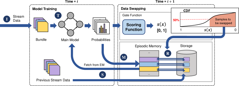
We describe how data swapping in CarM extends the current workflow of episodic memory (EM) in Figure 1. For ease of illustration, we assume that the input stream data is organized by consecutive tasks but CL learners do not necessarily rely on boundaries between tasks to perform training and update EM. There are three common stages involved in traditional EM methods, which proceed in order: data incoming, training, and EM updating. This workflow corresponds to many existing methods including TinyER (Chaudhry et al., 2019b), CBRS (Chrysakis & Moens, 2020), iCaRL (Rebuffi et al., 2017), BiC (Wu et al., 2019), and DER++ (Buzzega et al., 2020). Then, we add two additional key stages for data swapping: storage updating and storage sample retrieving.
-
•
Data incoming : The episodic memory maintains a subset of samples from previous tasks . When samples for a new task arrive, they are first enqueued into a stream buffer and later exercised for training. Different CL algorithms require different amounts of samples to be enqueued for training. The task-level learning relies on task boundaries, waiting until all ’s samples appear (Rebuffi et al., 2017; Wu et al., 2019). On the contrary, the batch-level learning initiates the training stage as soon as a batch of ’s samples in a pre-defined size is available (Chaudhry et al., 2019b; Shim et al., 2021; Chrysakis & Moens, 2020).
-
•
Training : The training combines old samples in EM with new samples in a stream buffer to compose a training bundle. The CL learner organizes the bundle into one or more mini-batches, where each mini-batch is a mixture of old and new samples. The mini-batch size and the ratio between the two types of samples within a mini-batch are configured by the learning algorithm. Typically, several mini-batches are constructed in the task-level learning. Learners may go over multiple passes given a bundle, trading off computation cost for accuracy.
-
•
EM updating : Once the training stage is completed, samples in the stream buffer are no longer new and represent a past experience, requiring EM to be updated with these samples. EM may have enough space to store all of them, but if it does not, the CL method applies a sampling strategy like reservoir sampling (Vitter, 1985) and greedy-balancing sampling (Prabhu et al., 2020) to select a subset of samples from EM as well as from the stream buffer to keep in EM. All prior works “discard” the samples which are not chosen to be kept in EM.
-
•
Storage updating : CarM flushes the stream data onto the storage before cleaning up the stream buffer for the next data incoming step. No loss of information occurs if the free space available in the storage is large enough for the stream data. However, if the storage is filled due to lack of capacity, we end up having victim samples to remove from the storage. In this case, we randomly choose samples to evict for each class while keeping the in-storage data class-balanced.
-
•
Storage sample retrieving : With the large number of samples maintained in the storage, data swapping replaces in-memory samples with in-storage samples during training to exercise abundant information preserved in the storage regarding past experiences. CarM collects various useful signals for each in-memory sample used in the training stage and determines whether to replace that sample or not. This decision is made by our generic gating function that selects a subset of the samples for replacement with effectively little runtime cost.
Since old samples for training are drawn directly from and a large pool of samples is always kept in the storage , the training phase is forced to have a boundary of sample selection restricted by the size of . The continual learning with data swapping that optimizes model parameters for old and new samples (and corresponding labels ) can hence be formulated as follows:
| (1) |
3.1 Minimizing Delay to Continual Model Training
The primary objective in our proposed design is hiding performance interference caused by the data swapping so that CarM incurs low latency during training. To that end, we propose two techniques that encompass in-storage sample retrieval and EM updating stages.
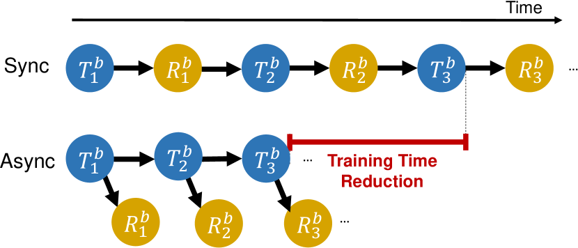
Asynchronous sample retrieval. Similar to the conventional learning practice, CarM maintains fetch workers performing data decoding and augmentation. As shown in Figure 1, CarM has an additional swap worker dedicated to deciding in-memory samples to evict and issuing I/O requests to bring new samples from storage into memory. In the CL workflow, the data retrieval stage has dependency on the training stage since training triggers the replacement of an in-memory sample when it is used as training input. To illustrate, we assume that the system has a single fetch worker to pre-process the training input bundle and creates mini-batch from the bundle – this pre-processing is incurred every time a sample is fetched for training. The swap worker identifies samples in EM to be replaced from mini-batch training () and then issues I/O requests to retrieve other samples from storage (). If we want to allow the next mini-batch training to exercise EM completely refreshed with the replaced samples, executions of and by definition must be serialized such that we have a sequence of , as shown in Figure 2 (Sync). However, committing to such strict serialized executions slows down training speed significantly, e.g., the second mini-batch training can start only after finishing up , which takes much longer time than with no retrieval of storage data as done in the traditional EM design. To prevent this performance degradation, CarM adopts asynchronous sample retrieval that runs the retrieval step in parallel with the subsequent training steps. By the asynchronous method, we keep the minimum possible dependency as shown in Figure 2 (Async), with an arbitrary not necessarily happened before . Apparently, this design choice poses a delay on applying in-storage samples to EM, making it possible for the next training steps to access some samples undergoing replacement. However, we found such accesses do not frequently occur, and the delay does not nullify the benefit that comes from data swapping.
In addition, when the swap worker retrieves in-storage samples and writes on memory, it may interfere with fetch workers that attempt to read samples from it for pre-processing. To mitigate such interference, CarM could opt for EM partitioning to parallelize read/write operations over independent partitions. With EM partitioning, only those operations that access the same partition need coordination, achieving concurrency against operations that access other partitions.
3.2 Data Swapping Policy by a Gate Function
The gate function in Figure 1 is a core component in CarM for adjusting I/O traffic. The gate, as guided by its decision logic, allows us to select a certain portion of samples to swap out from those EM samples drawn in the training stage. Having this control knob is of big practical importance as the maximum sustainable I/O traffic differs considerably among devices due to their in-use storage mediums with different characteristics (e.g., high-bandwidth flash drive vs low-bandwidth magnetic drive). At the same time, the gate is required to be effective with such partial data swapping in terms of accuracy in the subsequent training steps.
To facilitate this, we propose a sample scoring method that ranks the samples in the same mini-batch so that the training algorithm can decide at which point along the continuum of the ranks we can separate samples to swap from other samples to keep further in memory.
Score-based replacement. The score quantifies the relative importance of a trained sample to keep in EM with respect to other samples in the same mini-batch. Intuitively, a higher score means that the sample is in a higher rank, so is better “not” to be replaced if we need to reduce I/O traffic and vice versa. To this end, we define the gate function for sample, , as , where is a scoring function and is a scoring threshold, with both and between and . The threshold is determined by the proportion of the samples that we want to replace from the EM with samples in storage with the consideration of computational efficiency. It allows data swapping to match with I/O bandwidth available on the storage medium, and prevents the system from over-subscribing the bandwidth leading to I/O back-pressure and increased queueing time or under-subscribing the bandwidth leaving storage data exploited less opportunistically.
Policies. We design several swapping policies driven by the sample scoring method in the context of CL with data swapping for the first time. Specifically, we propose the following three policies:
(1) Random selects random samples to replace from EM. Its scoring function assigns 0 to the proportion of the samples randomly selected from a mini-batch while assigning 1 to the other samples.
(2) Entropy collects two useful signals for each sample produced during training: prediction correctness and the associated entropy. This policy prefers to replace the samples that are correctly predicted because these samples may not be much beneficial to improve the model in the near future. Furthermore, in this group of samples, if any specific sample has a lower entropy value than the other samples, the prediction confidence is relatively stronger, making it a better candidate for replacement. By contrast, for the samples that are incorrectly predicted, this policy prefers to “not” replace the samples that exhibit lower entropy, i.e., incorrect prediction with stronger confidence, since they may take longer to be predicted correctly. Thus, the scoring function with a model is defined as:
| (2) |
where , is an entropy function, and is the maximum entropy value.
(3) Dynamic combines Random and Entropy to perform the first half of training passes given a bundle with Random and the next half of the passes with Entropy. This policy is motivated by curriculum learning (Bengio et al., 2009), which gradually focuses on training harder samples as time elapses.
It is indeed possible to come up with a number of replacement policies, for which this paper introduces a few concrete examples. Regardless, designing the gate logic with more effective replacement policies is a promising research direction that we want to further explore in CarM.
4 Experiments
As CarM is broadly applicable to a variety of EM-based CL methods, we compare the performance with and without CarM in the methods of their own setups. We select seven methods as shown in Table 4.1, to cover several aspects discussed in Section 3 such as bundle boundary of learning (i.e., task-level vs batch-level) and number of passes taken per bundle. We discuss detailed reproducible settings in Section 5. For evaluation, we implement CarM in PyTorch 1.7.1 as a working prototype.
Datasets and metrics. Datasets include CIFAR subset—CIFAR10 (C10) and CIFAR100 (C100)—, ImageNet subset—ImageNet-100 (I100), Mini-ImageNet (100 classes) (MI100), and Tiny-ImageNet (200 classes) (TI200)—, and ImageNet-1000. We use two popular metrics, the final accuracy and the final forgetting (Chaudhry et al., 2018) averaged over classes, to reflect the performance of continual learning. Except for ImageNet-1000 that represents a significantly large-scale training, the results are averaged over five runs while each method assigns an equal of classes to each task. We also measure training speed measured from the time the training stage receives a bundle to the time it completes training the bundle.
Baselines and architectures. On top of each CL method, we vary the amount of data swapping to study the effectiveness of CarM in detail. Unless otherwise stated, CarM-N means that our swap worker is configured to replace N% of EM samples drawn by the training stage. All experiments are based on either ResNet or DenseNet neural networks, with all using the SGD optimizer as suggested by the original works, and use the entropy-based data swapping policy (i.e., Entropy) by default.
4.1 Results
| Metric | Method | ER | iCaRL | TinyER | BiC | GDumb | DER++ | RM | |
|---|---|---|---|---|---|---|---|---|---|
| (EM Sizes) | (2000/2000) | (2000/2000) | (300/500) | (2000/2000) | (500/4500) | (500/500) | (500/4500) | ||
| (Datasets) | (C100/I100) | (C100/I100) | (C100/MI100) | (C100/I100) | (C10/TI200) | (C10/TI200) | (C10/TI200) | ||
| CIFAR Subset | Acc. () | Original | 33.660.42 | 47.040.25 | 54.112.52 | 48.620.37 | 47.290.54 | 72.171.11 | 52.151.42 |
| \cdashline3-10 | CarM-50 | 54.000.49 | 48.390.41 | 59.992.12 | 62.400.40 | 52.641.64 | 90.050.38 | 66.660.75 | |
| CarM-100 | 54.930.46 | 49.480.53 | 61.832.50 | 63.070.48 | 53.721.06 | 90.580.30 | 67.810.51 | ||
| Fgt. () | Original | 57.600.54 | 22.380.30 | 16.042.91 | 20.210.65 | 22.140.83 | 24.451.81 | 23.032.86 | |
| \cdashline3-10 | CarM-50 | 32.130.72 | 17.180.53 | 11.91.13 | 13.400.86 | 20.921.63 | 3.380.22 | 9.630.40 | |
| CarM-100 | 32.280.55 | 16.730.65 | 9.441.96 | 12.160.69 | 21.181.49 | 2.780.55 | 11.032.28 | ||
| ImageNet Subset | Acc. () | Original | 65.621.48 | 79.951.12 | 56.912.32 | 83.050.66 | 42.250.44 | 19.381.41 | 21.840.54 |
| \cdashline3-10 | CarM-50 | 82.210.43 | 79.150.40 | 65.432.83 | 88.030.39 | 55.670.21 | 47.740.84 | 45.490.32 | |
| CarM-100 | 83.560.36 | 80.151.07 | 68.700.59 | 87.630.34 | 56.110.47 | 45.121.39 | 46.700.16 | ||
| Fgt. () | Original | 55.300.28 | 17.100.68 | 15.302.29 | 15.810.34 | 11.060.75 | 66.830.93 | 16.890.51 | |
| \cdashline3-10 | CarM-50 | 40.120.55 | 14.650.27 | 7.644.08 | 7.960.58 | 9.470.23 | 20.691.52 | 9.430.39 | |
| CarM-100 | 39.250.29 | 14.280.20 | 9.762.48 | 8.270.28 | 8.011.84 | 23.811.68 | 8.810.21 | ||
| ImageNet-1000 | Acc. () | Original | 40.47 | 56.69 | 46.41 | 77.04 | 38.14 | 12.11 | 24.08 |
| \cdashline3-10 | CarM-50 | 42.64 | 55.72 | 48.93 | 80.66 | 48.86 | 35.90 | 43.69 | |
| CarM-100 | 44.21 | 55.45 | 50.30 | 80.84 | 49.56 | 36.89 | 44.36 | ||
| Fgt. () | Original | 70.67 | 39.41 | 10.37 | 21.38 | 31.56 | 54.78 | 12.3 | |
| \cdashline3-10 | CarM-50 | 65.60 | 40.37 | 8.79 | 18.81 | 25.12 | 24.31 | 7.31 | |
| CarM-100 | 64.79 | 39.02 | 7.20 | 18.30 | 23.86 | 21.77 | 7.16 |
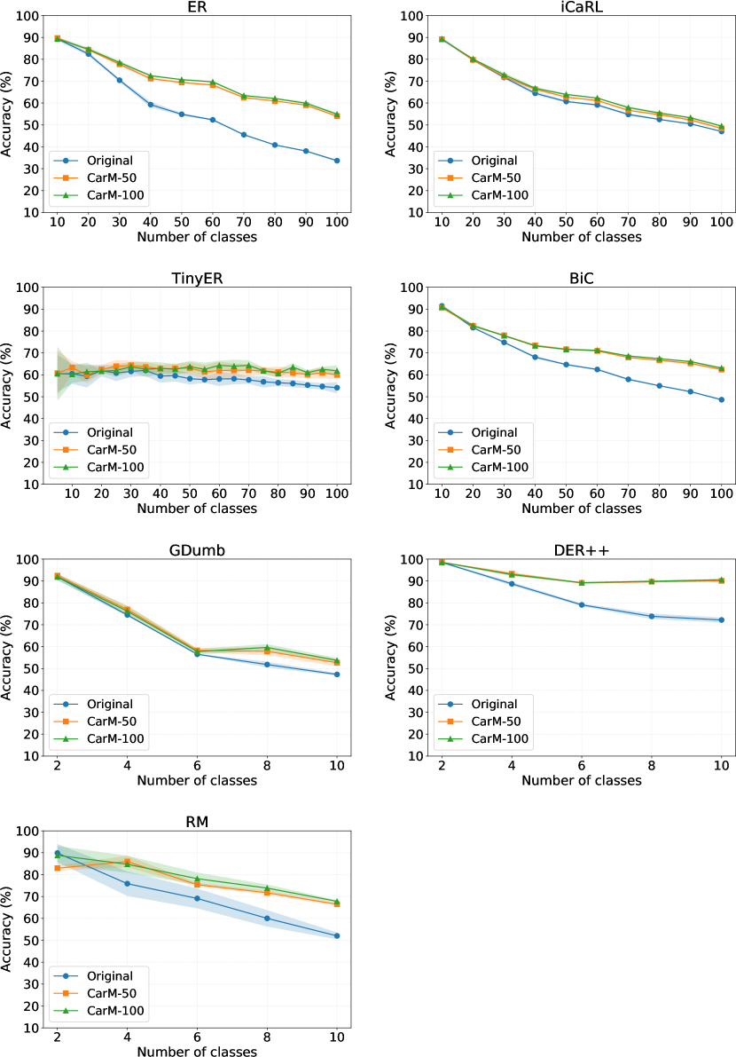
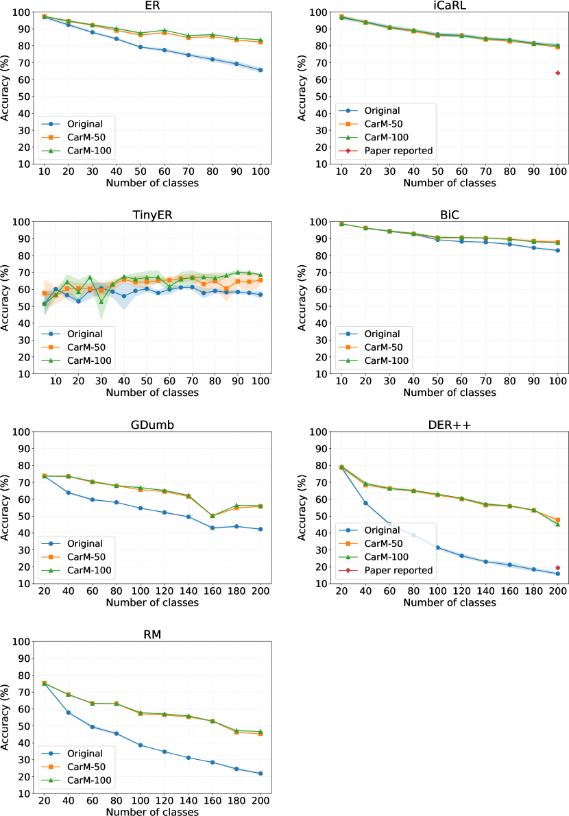
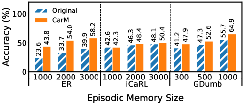
We compare existing methods with two CarM versions, CarM-50 that performs partial swapping for a half of the data and CarM-100 that performs full swapping. Table 4.1 presents the performance in terms of the top-1 accuracy (Acc.) and the forgetting score (Fgt.), except for ER, iCarL, and BiC that measure the top-5 accuracy for the ImageNet subset as done in the original works.
First, CarM-100 improves the accuracy remarkably over almost all of the methods under consideration, advancing the state-of-the-art performances for CIFAR and ImageNet datasets. The results clearly show the effectiveness of using the storage device in large capacity to allow CL to exploit abundant information of the previous tasks. Among the seven methods, CarM-100 delivers relatively larger accuracy gains for BiC (Wu et al., 2019), GDumb (Prabhu et al., 2020), DER++ (Buzzega et al., 2020), and RM (Bang et al., 2021) that take multi-passes on each training input. We believe that as long as old samples in EM are exercised more frequently for a new bundle to train (i.e., new samples plus old samples), data swapping can subsequently bring in more diverse samples from storage to take advantage of them. Regardless, although TinyER (Chaudhry et al., 2019b) is designed to take a single pass over new samples and thus exercise EM less aggressively, as applied with our techniques, it improves the accuracy by 7.72%, 11.79%, and 3.89% for CIFAR-100, Mini-ImageNet, and ImageNet-1000, respectively.
In comparison to CarM-100, CarM-50 obtains slightly lower accuracy across the models. We argue that such a small sacrifice in accuracy is indeed worthwhile when storage I/O bandwidth is the primary constraint. In CarM-50, with 50% lower I/O traffic caused by data swapping, the accuracy as compared to CarM-100 diminishes only by 1%, 0.6%, and 0.7% on average for CIFAR subset, ImageNet subset, and ImageNet-1000, respectively, providing an ability to trade-off small accuracy loss for substantial I/O traffic reduction. Similarly to the accuracy, our data swapping approaches considerably reduce forgetting scores over the majority of the original methods. Perhaps, one method that shows less promising results in Table 4.1 would be iCaRL (Rebuffi et al., 2017), where CarM makes the accuracy occasionally worse.
From the in-depth investigation of iCaRL in Appendix A.4.1, we observe that using data swapping and knowledge distillation at the same time cannot not deliver great accuracy. That is, as knowledge distillation may not be much compatible with data swapping, we revisit distillation-based CL methods (i.e., iCaRL, BiC, and DER++) when they are used along with data swapping in detail.
Knowledge distillation on CarM. Note that the ways to distill the knowledge of old data in iCaRL, BiC, and DER++ are all different (see Appendix A.4.1). Briefly speaking, in calculating loss for old data, iCaRL uses only soft labels obtained from an old classifier, whereas BiC and DER++ use both hard labels (i.e., ground truth) as well as soft labels. To investigate the effect of using these two types of loss, we first modify the loss function of iCaRL similarly to that of BiC, i.e., , and then show accuracy over varying values for all three distillation-based methods in Figure 3. For each method, we also include accuracy when increases incrementally over time as done in BiC.
| Method | ER | iCaRL | TinyER | BiC | GDumb | DER++ | RM |
|---|---|---|---|---|---|---|---|
| Random | 82.070.28 | 79.310.30 | 65.042.75 | 87.810.87 | 55.570.28 | 47.370.91 | 45.460.46 |
| Entropy | 82.210.43 | 79.150.40 | 65.432.83 | 88.030.93 | 55.670.21 | 47.740.84 | 45.490.32 |
| Dynamic | 82.940.43 | 79.140.31 | 65.042.75 | 87.790.88 | 55.510.74 | 47.532.09 | 45.800.25 |
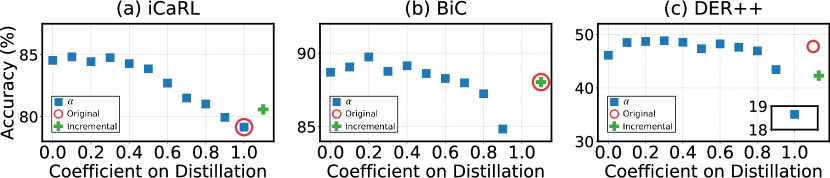
The results show that distillation-based methods with CarM significantly improve accuracy when the is very small. For iCaRL, compared to (i.e., no hard label loss as iCaRL does), we obtain 5.4 higher accuracy when (i.e., no distillation) and 5.7 higher accuracy when , which is the best result. Similarly, for BiC and DER++ with CarM, we found that the coefficient to be applied on the soft label loss does not necessarily be high (i.e., iCaRL) or managed complicatedly (i.e., BiC) to achieve higher accuracy. Please refer to Figure 6 for the CIFAR subset results.
Our best interpretation for the reason behind is as follows. The key assumption of knowledge distillation is that once the model is trained with a new task, the knowledge newly learned is supposed to generalize the task well and can be effectively transferable to subsequent task training. However, if the model is not sufficiently generalized for old tasks, using distillation losses extensively might be adverse—Data swapping attempts to correct decision boundaries driven by abundant in-storage samples to further generalize old tasks, but interfered by the knowledge distilled by the old models.
Comparison for data swapping policies. We compare the performance of the three data swapping policies proposed in Section 3.2 under CarM-50. As shown in Table 2, both Entropy and Dynamic outperform Random by 0.16% on average for ImageNet subset (see Table 10 for CIFAR subset). We highlight that our major contribution for gating mechanism is computational efficiency while matching with I/O bandwidth available on the storage medium, and the primary objective of exploring data swapping policies is establishing a good baseline for the gating mechanism. In this regard, we found that all three policies can serve as good baselines.
| Method | ER | iCaRL | TinyER | BiC | GDumb | DER++ | RM |
|---|---|---|---|---|---|---|---|
| Async | +0.7%/+2.9% | +0.5%/-2.7% | +3.3%/+5.5% | -0.3%/+1.7% | +3.3%/+0.1% | +0.3%/+2.4% | +2.3%/-0.9% |
| Sync | +30.2%/+21.3% | +70.5%/+62.0% | +11.3%/+10.7% | +20.0%/+33.8% | +52.1%/+7.6% | +71.6%/+38.8% | +25.9%/+2.6% |
Impact on training speed. Delay optimization techniques in Section 3.1 are intended to incur insignificant delay on training. To confirm this, we examine how training speed in CarM-50 changes over the original memory-only methods, measured as the percentage of wall-clock time (i.e., actual time taken) increase as applied with asynchronous (Async) vs synchronous sample retrieval (Sync). To consider the most challenging scenario, we make data entered into the stream buffer at a rate enough to keep training always busy with new mini-batches. As shown in Table 3, regardless of EM methods, the asynchronous version of CarM does not dramatically affect training speeds for both CIFAR and ImageNet subsets. By contrast, the synchronous version slows down training time up to 71.6% for CIFAR subset and 62.0% for ImageNet subset. Regardless of the version in use, in-memory samples undergoing data swapping are rarely drawn in the subsequent training steps since the size of an episodic memory size is typically much larger than the size of a training batch. Therefore, no difference in accuracy is observed between the two version.
4.2 Ablation Study
We present an ablation study using four methods (TinyER, BiC, DER++, and RM) that represent the state-of-the-art in each type of EM methodologies, using the CIFAR subset.
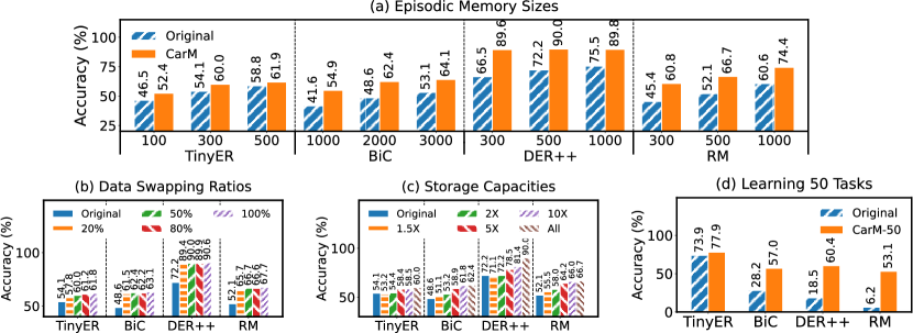
Size of EM. To confirm performance benefits over using different memory sizes, we empirically evaluate CarM-50 over varying EM sizes and show the average accuracy in Figure 4(a). In all cases, CarM-50 outperforms the existing methods, with BiC, DER++, and RM having relatively higher accuracy increases. Moreover, we observe that data swapping delivers better accuracy over conventional memory-only approaches using much smaller memory. For example, CarM-50 with DER++ on EM size 300 shows higher accuracy than pure DER++ on EM size 1000, and CarM-50 with TinyER on EM size 300 shows higher accuracy than pure TinyEM on EM size 500. Therefore, it turns out that data swapping could help reduce the EM size without hurting the accuracy of existing methods in both the multi-pass method and single-pass method.
Data swapping ratio. We present results with different swapping ratios to show that our gate model indeed brings out meaningful benefits over using different I/O bandwidths. To that end, Figure 4(b) shows the change in accuracy when our gating policy decreases the swapping ratio down to 20% (CarM-20) or increases it up to 80% (CarM-80). Obviously, at CarM-80 in high swapping ratio, the accuracy across the four EM methods gets very close to the accuracy obtained in full swapping. A surprising result is that even at CarM-20 in 20% data swapping, the accuracy is very comparable to when we allow higher data swapping ratios. The results indicate that our method would be effective even when applied to the system with low-bandwidth storage.
Size of storage. As local storage cannot store all the past data, the system must discard some old samples once the storage is fully occupied. Figure 4(c) shows accuracy degradation in CarM-50 when storage capacity is limited to 1.5–10 of the EM size. The results show that data swapping improves performance over traditional approaches even with using 50% larger capacity for the storage.
Large number of tasks. One pressing issue on CL is learning a large number of tasks as it is required to keep the knowledge learned in the remote past. To evaluate this aspect, we split CIFAR-100 (100 classes) into 50 tasks and run with the four methods. As Figure 4(d) shows, CarM significantly outperforms the baselines, showing the potential for long-term continual model training.
5 Conclusion
We alleviate catastrophic forgetting by integrating traditional episodic memory-based continual learning methods with device-internal data storage, named CarM. We design data swapping strategies to improve model accuracy by dynamically utilizing a large amount of the past data available in the storage. Our swapping mechanism addresses the cumbersome performance hurdle incurred by slow storage access, and hence continual model training is not dramatically affected by data transfers between memory and storage. We show the effectiveness of CarM using seven well-known methods on standard datasets, over varying memory sizes, storage sizes, and data swapping ratios.
Reproducibility Statement
We take the reproducibility of the research very seriously. Appendix hence includes detailed information necessary for reproducing all the experiments performed in this work, as follows:
-
•
Appendix A.1 describes the implementation details of building CarM.
-
•
Appendix A.2 specifies dataset information used in the experiments (e.g., the number of tasks and the number of classes per task).
-
•
Appendix A.3 provides experimental details (e.g., metrics and hyper-parameters).
-
•
Appendix A.3.4 presents detailed specification of machines (e.g., GPU model) used in the experiments.
Our source code is available at https://github.com/supersoob/CarM, where we include running environments and configuration files for all the experiments that make it possible to reproduce the results reported in this paper with minimal effort.
Ethics Statement
All continual learning (CL) methods including the proposed one would adapt and extend the already trained AI model to recognize better with the streamed data. The CL methods will expedite the deployment of AI systems to help humans by its versatility of adapting to a new environment out of the factory or research labs. As all CL methods, however, would suffer from adversarial streamed data as well as data bias, which may cause ethnic, gender or biased gender issues, the proposed method would not be an exception. Although the proposed method has no intention to allow such problematic cases, the method may be exposed to such threats. Relentless efforts should be made to develop mechanisms to prevent such usage cases in order to make the continuously updating machine learning models safer and enjoyable to be used by humans.
References
- (1) Python asynchronous i/o. https://docs.python.org/3.8/library/asyncio.html.
- (2) Python manager. https://docs.python.org/3.8/library/multiprocessing.html#managers.
- (3) Python multiprocessing. https://docs.python.org/3.8/library/multiprocessing.html.
- (4) Python shared memory. https://docs.python.org/3.8/library/multiprocessing.shared_memory.html.
- Aljundi et al. (2019) Rahaf Aljundi, Min Lin, Baptiste Goujaud, and Yoshua Bengio. Gradient based sample selection for online continual learning. In NIPS, 2019.
- Ananthanarayanan et al. (2012) Ganesh Ananthanarayanan, Ali Ghodsi, Andrew Warfield, Dhruba Borthakur, Srikanth Kandula, Scott Shenker, and Ion Stoica. Pacman: Coordinated memory caching for parallel jobs. In USENIX NSDI, pp. 267–280, 2012.
- Bang et al. (2021) Jihwan Bang, Heesu Kim, YoungJoon Yoo, Jung-Woo Ha, and Jonghyun Choi. Rainbow memory: Continual learning with a memory of diverse samples. In CVPR, 2021.
- Bengio et al. (2009) Yoshua Bengio, Jérôme Louradour, Ronan Collobert, and Jason Weston. Curriculum learning. In ICML, 2009.
- Borsos et al. (2020) Zalán Borsos, Mojmír Mutnỳ, and Andreas Krause. Coresets via bilevel optimization for continual learning and streaming. In NIPS, 2020.
- Buzzega et al. (2020) Pietro Buzzega, Matteo Boschini, Angelo Porrello, Davide Abati, and SIMONE CALDERARA. Dark experience for general continual learning: a strong, simple baseline. In NIPS, 2020.
- Castro et al. (2018) Francisco M. Castro, Manuel J. Marin-Jimenez, Nicolas Guil, Cordelia Schmid, and Karteek Alahari. End-to-end incremental learning. In ECCV, 2018.
- Chaudhry et al. (2018) Arslan Chaudhry, Puneet K. Dokania, Thalaiyasingam Ajanthan, and Philip H. S. Torr. Riemannian walk for incremental learning: Understanding forgetting and intransigence. In ECCV, 2018.
- Chaudhry et al. (2019a) Arslan Chaudhry, Marc’Aurelio Ranzato, Marcus Rohrbach, and Mohamed Elhoseiny. Efficient lifelong learning with A-GEM. In ICLR, 2019a.
- Chaudhry et al. (2019b) Arslan Chaudhry, Marcus Rohrbach, Mohamed Elhoseiny, Thalaiyasingam Ajanthan, Puneet K Dokania, Philip HS Torr, and Marc’Aurelio Ranzato. On tiny episodic memories in continual learning. arXiv preprint arXiv:1902.10486, 2019b.
- Chrysakis & Moens (2020) Aristotelis Chrysakis and Marie-Francine Moens. Online continual learning from imbalanced data. In ICML, volume 119, pp. 1952–1961, 2020.
- Cong et al. (2020) Yulai Cong, Miaoyun Zhao, Jianqiao Li, Sijia Wang, and Lawrence Carin. GAN memory with no forgetting. In NIPS, 2020.
- Douillard et al. (2020) Arthur Douillard, Matthieu Cord, Charles Ollion, Thomas Robert, and Eduardo Valle. Podnet: Pooled outputs distillation for small-tasks incremental learning. In ECCV, 2020.
- Fini et al. (2020) Enrico Fini, Stéphane Lathuilière, Enver Sangineto, Moin Nabi, and Elisa Ricci. Online continual learning under extreme memory constraints. In ECCV, 2020.
- Gepperth & Hammer (2016) Alexander Gepperth and Barbara Hammer. Incremental learning algorithms and applications. In ESANN, 2016.
- Hayes et al. (2020) Tyler L Hayes, Kushal Kafle, Robik Shrestha, Manoj Acharya, and Christopher Kanan. Remind your neural network to prevent catastrophic forgetting. In ECCV, 2020.
- Hildebrand et al. (2020) Mark Hildebrand, Jawad Khan, Sanjeev Trika, Jason Lowe-Power, and Venkatesh Akella. Autotm: Automatic tensor movement in heterogeneous memory systems using integer linear programming. In ASPLOS, pp. 875–890, 2020.
- Hu et al. (2019) Wenpeng Hu, Zhou Lin, Bing Liu, Chongyang Tao, Zhengwei Tao, Jinwen Ma, Dongyan Zhao, and Rui Yan. Overcoming catastrophic forgetting via model adaptation. In ICLR, 2019.
- Huang et al. (2020) Chien-Chin Huang, Gu Jin, and Jinyang Li. Swapadvisor: Pushing deep learning beyond the gpu memory limit via smart swapping. In ASPLOS, pp. 1341–1355, 2020.
- Jin et al. (2018) Hai Jin, Bo Liu, Wenbin Jiang, Yang Ma, Xuanhua Shi, Bingsheng He, and Shaofeng Zhao. Layer-centric memory reuse and data migration for extreme-scale deep learning on many-core architectures. In ACM TACO, volume 15, pp. 1–26, 2018.
- Jin et al. (2020) Xisen Jin, Junyi Du, and Xiang Ren. Gradient based memory editing for task-free continual learning. arXiv preprint arXiv:2006.15294, 2020.
- Kang et al. (2020) Dongmin Kang, Yeonsik Jo, Yeongwoo Nam, and Jonghyun Choi. Confidence calibration for incremental learning. In IEEE Access, volume 8, pp. 126648–126660, 2020.
- Kirkpatrick et al. (2017) James Kirkpatrick, Razvan Pascanu, Neil Rabinowitz, Joel Veness, Guillaume Desjardins, Andrei A Rusu, Kieran Milan, John Quan, Tiago Ramalho, Agnieszka Grabska-Barwinska, et al. Overcoming catastrophic forgetting in neural networks. In PNAS, 2017.
- Lee et al. (2017) Sang-Woo Lee, Jin-Hwa Kim, Jaehyun Jun, Jung-Woo Ha, and Byoung-Tak Zhang. Overcoming catastrophic forgetting by incremental moment matching. In NIPS, 2017.
- Li & Hoiem (2017) Zhizhong Li and Derek Hoiem. Learning without forgetting. In IEEE Trans. PAMI, 2017.
- Liu et al. (2018) Xialei Liu, Marc Masana, Luis Herranz, Joost Van de Weijer, Antonio M Lopez, and Andrew D Bagdanov. Rotate your networks: Better weight consolidation and less catastrophic forgetting. In ICPR, 2018.
- Liu et al. (2020) Yaoyao Liu, Yuting Su, An-An Liu, Bernt Schiele, and Qianru Sun. Mnemonics training: Multi-class incremental learning without forgetting. In CVPR, pp. 12245–12254. Computer Vision Foundation / IEEE, 2020.
- Lopez-Paz & Ranzato (2017) David Lopez-Paz and Marc’Aurelio Ranzato. Gradient episodic memory for continual learning. In NIPS, volume 30, pp. 6467–6476, 2017.
- Mallya et al. (2018) Arun Mallya, Dillon Davis, and Svetlana Lazebnik. Piggyback: Adapting a single network to multiple tasks by learning to mask weights. In ECCV, 2018.
- McCloskey & Neal (1989) M. McCloskey and Neal. Catastrophic interference in connectionist networks: The sequential learning problem. In Psychology of Learning and Motivation, volume 24, pp. 109–165, 1989.
- Oh et al. (2012) Yongseok Oh, Jongmoo Choi, Donghee Lee, and Sam H Noh. Caching less for better performance: balancing cache size and update cost of flash memory cache in hybrid storage systems. In USENIX FAST, volume 12, pp. 25, 2012.
- Parisi et al. (2018) German Parisi, Ronald Kemker, Jose L. Part, Christopher Kanan, and Stefan Wermter. Continual lifelong learning with neural networks: A review. In Neural Networks, 2018.
- Peng et al. (2020) Xuan Peng, Xuanhua Shi, Hulin Dai, Hai Jin, Weiliang Ma, Qian Xiong, Fan Yang, and Xuehai Qian. Capuchin: Tensor-based gpu memory management for deep learning. In ASPLOS, pp. 891–905. ACM, 2020.
- Prabhu et al. (2020) Ameya Prabhu, Philip HS Torr, and Puneet K Dokania. GDumb: A simple approach that questions our progress in continual learning. In ECCV, 2020.
- Ratcliff (1990) Roger Ratcliff. Connectionist models of recognition memory: Constraints imposed by learning and forgetting functions. In Psychological Review, volume 97, pp. 285–308, 1990.
- Rebuffi et al. (2017) Sylvestre-Alvise Rebuffi, Alexander Kolesnikov, Georg Sperl, and Christoph H. Lampert. iCaRL: Incremental classifier and representation learning. In CVPR, 2017.
- Ren et al. (2021) Jie Ren, Jiaolin Luo, Kai Wu, Minjia Zhang, Hyeran Jeon, and Dong Li. Sentinel: Efficient tensor migration and allocation on heterogeneous memory systems for deep learning. In IEEE HPCA, pp. 598–611. IEEE, 2021.
- Rhu et al. (2016) Minsoo Rhu, Natalia Gimelshein, Jason Clemons, Arslan Zulfiqar, and Stephen W. Keckler. vdnn: Virtualized deep neural networks for scalable, memory-efficient neural network design. In MICRO, pp. 1–13. IEEE Computer Society, 2016.
- Seff et al. (2017) Ari Seff, Alex Beatson, Daniel Suo, and Han Liu. Continual learning in generative adversarial nets. arXiv preprint arxiv:1705.08395, 2017.
- Shim et al. (2021) Dongsub Shim, Zheda Mai, Jihwan Jeong, Scott Sanner, Hyunwoo Kim, and Jongseong Jang. Online class-incremental continual learning with adversarial shapley value. In AAAI, volume 35, pp. 9630–9638, 2021.
- Shin et al. (2017) Hanul Shin, Jung Kwon Lee, Jaehong Kim, and Jiwon Kim. Continual learning with deep generative replay. In NIPS, 2017.
- van de Ven & Tolias (2018) Gido M van de Ven and Andreas S Tolias. Three continual learning scenarios and a case for generative replay. In NIPS Workshop on Continual Learning, 2018.
- Vitter (1985) Jeffrey S Vitter. Random sampling with a reservoir. In ACM TOMS, volume 11, pp. 37–57, 1985.
- Wang et al. (2018) Linnan Wang, Jinmian Ye, Yiyang Zhao, Wei Wu, Ang Li, Shuaiwen Leon Song, Zenglin Xu, and Tim Kraska. Superneurons: Dynamic gpu memory management for training deep neural networks. In PPoPP, pp. 41–53, 2018.
- Wang et al. (2019) Yue Wang, Ziyu Jiang, Xiaohan Chen, Pengfei Xu, Yang Zhao, Yingyan Lin, and Zhangyang Wang. E2-train: Training state-of-the-art cnns with over 80% energy savings. In NIPS, pp. 5139–5151. Curran Associates, Inc., 2019.
- Welling (2009) Max Welling. Herding dynamical weights to learn. In ICML, pp. 1121–1128, 2009.
- Wu et al. (2018) Chenshen Wu, Luis Herranz, Xialei Liu, Yaxing Wang, Joost Van de Weijer, and Bogdan Raducanu. Memory Replay GANs: learning to generate images from new categories without forgetting. In NIPS, 2018.
- Wu et al. (2019) Yue Wu, Yinpeng Chen, Lijuan Wang, Yuancheng Ye, Zicheng Liu, Yandong Guo, and Yun Fu. Large scale incremental learning. In CVPR, 2019.
- Zaharia et al. (2010) Matei Zaharia, Mosharaf Chowdhury, Michael J Franklin, Scott Shenker, Ion Stoica, et al. Spark: Cluster computing with working sets. In USENIX Workshop on HotCloud, pp. 95, 2010.
- Zenke et al. (2017) Friedemann Zenke, Ben Poole, and Surya Ganguli. Continual learning through synaptic intelligence. In ICML, 2017.
Appendix A Appendix
A.1 Implementation Details
First, we describe implementation details about the two components of the proposed method: swap worker and episodic memory. Then, we describe the details about PyTorch integration of our implementation for ease of use.
Swap worker. CarM implements the swap worker through multiprocessing (pyt, ) in popular Python standard library so that data swapping is running in parallel with PyTorch’s default fetch workers dedicated to data decoding and augmentation. The swap worker uses asyncio (asy, ) to asynchronously load samples from storage to memory, effectively overlapping high-latency I/O operations with other CarM-related operations, such as image decoding, sample replacement on EM, and entropy calculation. The swap worker issues multiple data swapping requests without spinning on or being blocked by I/O. As a result, it is sufficient to have only one swap worker for CarM in the system.
Episodic memory. There are various ways to implement EM to be shared between fetch workers and the swap worker. The current system favors flexibility over performance, so we opt for implementing EM as a shared object provided by Manager (man, ) in the Python standard library (multiprocessing.managers), which is based on message passing in the server-client semantics. In terms of flexibility, the Manager does not require the clients (i.e., fetch workers and swap workers) to define the exact data layout in the EM address space or coordinate for potential memory resizing to accommodate raw samples of different sizes (e.g., image resolutions). Hence, it is sufficient for the client workers to perform reads and writes on EM using indexes on the EM samples. An alternative yet obviously higher-performance implementation would be using multiprocessing.shared_memory (sha, ), which enables direct reads and writes on EM by exposing a common region of memory to the processes. Despite good performance, this method is less flexible as all processes should be aware of the data layout in a designated EM address range precisely at runtime, thus requiring additional coordination for sample lookups and EM resizing. As our system evolves, we ultimately want to combine the best of both methods to promise both flexibility and performance.
A.2 Datasets
Each baseline is evaluated on its own dataset used in the original work. The first rows of Table 4 and Table 5 show datasets used in the CIFAR subset and the ImageNet subset, respectively, for all baselines. ImageNet-100 is a ImageNet ILSVRC2012 subset used in iCaRL, which contains images in the same resolution as those in the original ImageNet ILSVRC2012. Other datasets used as the ImageNet subset have smaller image resolution than the original one (e.g., 6464 for Tiny-ImageNet, 8484 for Mini-ImageNet). In addition, we trained all baselines on ImageNet-1000 to verify the effectiveness of CarM on a large-scale dataset. We note that only ER, iCaRL, and BiC have been compared using the ImageNet-1000 dataset in the literature (Wu et al., 2019).
Datasets are split as done in the original work. The second and third rows of Table 4 and Table 5 show the detailed information on the splitting strategy. For all baselines, the ImageNet-1000 dataset is split into 10 tasks, each with 100 classes. Note that all datasets are non-blurry, meaning that each task consists of its own set of classes and samples belonging to a previous task never appear in the next tasks. Since the experimental results are highly sensitive to the class order in the continuous tasks to train, we follow the same class order used in the original works.
A.3 Experimental Details
We present the effectiveness of the proposed CarM using seven CL methods of their own setups. This section discusses detailed settings for each method so that the results are reproducible by our source code. We first describe the metrics used for the evaluations.
| ER | iCaRL | TinyER | BiC | GDumb | DER++ | RM | |
|---|---|---|---|---|---|---|---|
| Dataset | CIFAR-100 | CIFAR-100 | CIFAR-100 | CIFAR-100 | CIFAR-10 | CIFAR-10 | CIFAR-10 |
| # of Tasks | 10 | 10 | 20 | 10 | 5 | 5 | 5 |
| # of Classes per Task | 10 | 10 | 5 | 10 | 2 | 2 | 2 |
| ER | iCaRL | TinyER | BiC | GDumb | DER++ | RM | |
|---|---|---|---|---|---|---|---|
| Dataset | ImageNet-100 | ImageNet-100 | Mini-ImageNet | ImageNet-100 | Tiny-ImageNet | Tiny-ImageNet | Tiny-ImageNet |
| # of Tasks | 10 | 10 | 20 | 10 | 10 | 10 | 10 |
| # of Classes per Task | 10 | 10 | 5 | 10 | 20 | 20 | 20 |
A.3.1 Metrics
Final accuracy. Final accuracy is an average accuracy over all classes observed after the last task training is done.
Final forgetting. Forgetting indicates how much each task has been forgotten while training new tasks (Chaudhry et al., 2018). Forgetting for a task is calculated by comparing the best accuracy observed over task insertions to the final accuracy of the task when training is over. Final forgetting is an average forgetting across all tasks when training is over.
A.3.2 Baseline Details
-
•
ER (Ratcliff, 1990) combines all samples in the current stream buffer and the current EM, and passes them over to the model as a training set, i.e., training bundle. There is no algorithmic optimization applied to the model itself. We manage EM as a ring buffer that assigns EM space equally over all classes observed so far. We use the same hyper-parameters and loss function (binary cross-entropy loss) as used in iCaRL.
-
•
iCaRL (Rebuffi et al., 2017) uses three algorithmic optimizations: distillation loss, herding, and nearest-mean-of-exemplar classification. To transfer the information of old tasks, iCaRL leverages the distillation loss using logits obtained from the most recently trained model for old classes: this loss information is considered as the ground truth for old classes. Herding is its own EM management method, which populates the samples whose feature vectors are the closest to the average feature vector overall stream data for each class. iCaRL allocates EM space equally overall observed classes.
-
•
TinyER (Chaudhry et al., 2019b) explores four EM management strategies named reservoir, ring buffer, k-means, and mean of features. We adopt the reservoir in the experiments because it shows overall the highest performance in the original paper. Similar to ER, TinyER retrieves old samples from EM without other optimizations on the model itself. TinyER is batch-level learning and focuses on an extremely online setup that takes a single pass for every streamed batch.
-
•
BiC (Wu et al., 2019) runs bias correction on the last layer of the neural network, structured as fully connected layer, to mitigate data imbalance problem between old samples and new samples. The data imbalance is an inherent problem due to the limited size of EM, and it gets worse as we have a larger number of consecutive classes to train. Similar to iCaRL, BiC opts for distillation loss, but its entire loss function is a mixture of distillation loss and cross-entropy loss that is directly calculated from some reserved samples for old classes.
-
•
GDumb (Prabhu et al., 2020) is a simple rehearsal-based method that uses only the memory to train the model. The memory management is done via greedy balanced sampling, where GDumb tries to keep each class balanced by evicting data categorized into the majority class out of EM. Unlike other methods, the model is trained from scratch for inference and then discarded every time the memory is updated. GDumb uses cosine annealing learning-rate scheduler and cross-entropy loss for gradient descend.
-
•
DER++ (Buzzega et al., 2020) is one of rehearsal-based methods with knowledge distillation. Unlike other methods, this approach retains logits (along with samples) in EM for knowledge distillation. For knowledge distillation, DER++ calculates euclidean distance between the logits stored in EM and the logits generated by the current network. To enable data swapping on DER++, we store the logits in the storage along with samples.
-
•
RM (Bang et al., 2021) uses the same backbone as GDumb, but it improves memory update policy and training method over GDumb. For memory management, RM calculates the uncertainty of each sample and tries to fill the memory with samples in a wide spectrum that ranges from robust samples with low uncertainity to fragile samples with high uncertainity while keeping the classes balanced. In addition, data augmentation (DA) is proposed to advance the original RM implementation. We use RM without DA to apply data swapping in our work, but we include some results of RM with DA in Section A.4.4.
Reproduction. We use reported numbers from the original paper for DER++ on Tiny-ImageNet (Buzzega et al., 2020). For iCaRL, we believe we faithfully implement its details, but could not reach the accuracy reported in the paper.
As far as we know, there is no PyTorch source code that reproduces iCaRL on both CIFAR-100 and ImageNet-100 datasets. In our implementation for iCaRL, we refer to a PyTorch version written by the PodNet authors (Douillard et al., 2020) as they achieve the most comparable results. We use the results obtained from the referred version rather than the reported results, because compared to the reported accuracy, the obtained accuracy is nearly the same for CIFAR-100 and higher for ImageNet-100.
| ER | iCaRL | TinyER | BiC | GDumb | DER++ | RM | |
| Learning Level | Task | Task | Batch | Task | Task | Task | Task |
| Model | ResNet32 | ResNet32 | ReducedResNet18 | ResNet32 | ResNet18 | ResNet18 | ResNet18 |
| # Passes per Bundle | 70 | 70 | 1 | 250 | 256 | 50 | 256 |
| EM Size | 2000 | 2000 | 300 | 2000 | 500 | 500 | 500 |
| Batch Size | 128 | 128 | 10 | 128 | 16 | 32 | 16 |
| Learning Rate | 2.0 | 2.0 | 0.1 | 0.1 | 0.05 | 0.03 | 0.05 |
| Weight Decay | 1e-5 | 1e-5 | 0 | 2e-4 | 1e-6 | 0 | 1e-6 |
| TI / CI | CI | CI | TI | CI | CI | CI | CI |
| ER | iCaRL | TinyER | BiC | GDumb | DER++ | RM | |
| Learning Level | Task | Task | Batch | Task | Task | Task | Task |
| Model | ResNet18 | ResNet18 | ResNet18 | ResNet18 | DenseNet100 | ResNet18 | DenseNet100 |
| # Passes per Bundle | 60 | 60 | 1 | 100 | 128 | 100 | 128 |
| EM Size | 2000 | 2000 | 500 | 2000 | 4500 | 500 | 4500 |
| Batch Size | 128 | 128 | 10 | 256 | 16 | 32 | 16 |
| Learning Rate | 2.0 | 2.0 | 0.1 | 0.1 | 0.05 | 0.03 | 0.05 |
| Weight Decay | 1e-5 | 1e-5 | 0 | 1e-4 | 1e-6 | 0 | 1e-6 |
| TI / CI | CI | CI | TI | CI | TI | CI | CI |
| ER | iCaRL | TinyER | BiC | GDumb | DER++ | RM | |
| Learning Level | Task | Task | Batch | Task | Task | Task | Task |
| Model | ResNet18 | ResNet18 | ResNet18 | ResNet18 | DenseNet100 | ResNet18 | DenseNet100 |
| # Passes per Bundle | 60 | 140 | 1 | 100 | 128 | 100 | 128 |
| EM Size | 20000 | 20000 | 20000 | 20000 | 20000 | 20000 | 20000 |
| Batch Size | 128 | 128 | 32 | 256 | 16 | 16 | 16 |
| Learning Rate | 2.0 | 2.0 | 0.1 | 0.1 | 0.05 | 0.03 | 0.05 |
| Weight Decay | 1e-5 | 1e-5 | 0 | 1e-4 | 1e-6 | 0 | 1e-6 |
| TI / CI | CI | CI | TI | CI | TI | CI | CI |
A.3.3 Hyper-parameters
We follow hyper-parameters presented in the original works: we did not perform hyper-parameter search for the baselines. Table 6, Table 7, and Table 8 present all the details on the hyper-parameters.
Although DER++ updates EM in batch-level and does not consider task boundary, for a larger dataset than MNIST, the original paper chooses to takes multiple passes per bundle. So, we deem DER++ to be a task-level learning method as long as we use CIFAR-100 and Tiny ImageNet as its training dataset. Here, TI and CI denote task-incremental learning and class-incremental learning, respectively. TI is an easy and simplified scenario, where the task ID is given at both training and inference. In TI setting, the model can classify the input among the classes that belong to the provided task ID. On the contrary, CI is the setting where the task ID is unknown during inference, which is a more realistic case than TI.
A.3.4 Detailed Specification of Machines
Our experiments are performed on machines with HW specification as presented in Table 9. These machines are also used in measuring the impact on training speed with data swapping.
| Machine Specs | |
|---|---|
| CPU | Intel(R) Xeon(R) Gold 6226 CPU @ 2.70 GHz 2 |
| GPU | NVIDIA Geforce RTX 2080Ti (11 GB) 4 |
| RAM | 128 GB, 2666 MHz |
| SSD | Intel SSD D3 Series 480 GB |
| HDD | Western Digital Ultrastar DC HC310 4 TB |
A.4 Additional Results
A.4.1 Distillation Analysis
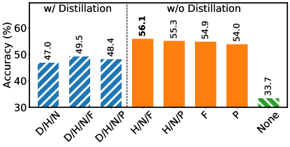
Effectiveness of features of iCaRL on CarM. We explore iCaRL by measuring accuracy for all possible 32 combinations based on its algorithmic features, i.e., knowledge distillation (D), herding (H), and nearest-mean-of-exemplars (N), along with our CarM-100 (F) or CarM-50 (P). In Figure 5, we show eight combinations that are sufficient to support the three interesting findings. First, data swapping without distillation (orange bars) outperforms the other combinations including pure iCaRL (blue and green bars). Second, for combinations with distillation, applying data swapping does not deliver great accuracy (D/H/N vs the other two in blue bars). Finally, data swapping does not seem to necessitate sophisticated algorithmic features (F&H vs D/H/N), inferring a model simplification potential for episodic memory.
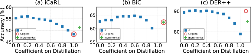
Knowledge distillation on CarM. Figure 6 show accuracy for CIFAR subset while varying values in for iCaRL, BiC, and DER++. We can make the same conclusions as discussed in the ‘Knowledge distillation on CarM’ paragraph of Section 4.1. Below, we describe how each distillation-based method can be transformed into the presented model for loss calculation.
The original loss function of iCaRL (Rebuffi et al., 2017) is defined as:
| (3) |
where is the output of the old model, is the output of the current model, is a set of old classes and is the set of new classes.
For distillation, it uses soft targets from the previous model for old classes of all current training set. As a result, training the current model heavily relies on the performance of the previous model. Especially, when data that belongs to old classes replays, since the target of loss is only soft output from the previous model, it is likely that the similar soft output from the old model is repeatedly distilled without the correct hard label. Due to such aggressive distillation, iCaRL cannot take an advantage of CarM, which enables to replay and train abundant old data, hindering positive decision boundary corrections. That is, the wrongly predicted samples from the old model will be predicted wrongly also in the future even if they are replayed several times by CarM. BiC and DER++ use distillation loss, however, unlike iCaRL, they provide a loss term of which target for old classes is ground truth, the correct hard label. As a result, BiC and DER++ could get higher accuracies with CarM. To evaluate Figure 3 and Figure 6, we modified the loss function of iCaRL, adding another binary cross entropy that uses the ground truth as the target, which is referred to hard label loss, as following:
| (4) |
Since BiC and DER++ already have its own hard label loss, we did not modify loss function. Note that when is set to 1.0 in BiC, it is unable to train any new data, which is unrealistic situation. So we excluded the result of of BiC.
| Method | ER | iCaRL | TinyER | BiC | GDumb | DER++ | RM |
|---|---|---|---|---|---|---|---|
| Random | 54.080.50 | 48.270.51 | 59.641.91 | 62.530.25 | 52.391.80 | 89.820.11 | 66.910.81 |
| Entropy | 54.000.49 | 48.390.41 | 59.992.12 | 62.400.40 | 52.641.64 | 90.050.38 | 66.660.78 |
| Dynamic | 54.160.37 | 48.390.57 | 59.620.93 | 62.320.24 | 52.922.09 | 89.920.22 | 66.610.73 |
A.4.2 Incremental Accuracy of Table 1 in the Main Paper
Incremental accuracy. We here report incremental accuracy as an additional performance metric. Incremental accuracy is a set of average accuracy over classes observed so far after training each task.
Figure 11 and Figure 11 show the incremental accuracy of Table 1 in the main paper. We also mark the accuracy from original paper of iCaRL on CIFAR-100, iCaRL on ImageNet-100, BiC on ImageNet-100 and DER++ on Tiny-ImageNet. In general, the more tasks (classes) come, the larger gap of accuracy between original and CarM. This implies that running on CarM could better mitigate the catastrophic forgetting for long-term training.
A.4.3 Ablation Study on ER, iCaRL, and GDumb
We report the results for an ablation study on ER, iCaRL, and GDumb, which were not presented in the main paper. Figure 7 shows accuracy over varying EM sizes, Figure 10 shows accuracy over varying swapping ratios, Figure 10 shows accuracy over varying storage capacity, and Figure 10 shows accuracy with learning 50 tasks. In general, we found the similar observations as discussed in Section 4.2.
floatrowsep=qquad
{floatrow}[3]\ffigbox[\FBwidth]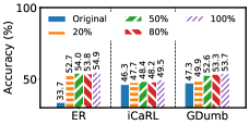 \ffigbox[\FBwidth]
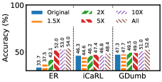 \ffigbox[\FBwidth]
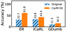
A.4.4 Results of RM with Data Augmentation
We implement RM with data augmentation and show the results in Table 11 using CIFAR-10 dataset. Both CarM and CarM-50 improves accuracy significantly over the baseline method.
| Original | CarM-50 | CarM-100 | |
|---|---|---|---|
| Final Accuracy | 68.071.57 | 84.070.83 | 84.850.42 |
| Final Forgetting | 15.091.72 | 5.120.89 | 4.360.95 |
| Method | ER | iCaRL | TinyER | BiC | GDumb | DER++ | RM |
|---|---|---|---|---|---|---|---|
| Original | 33.87 | 46.54 | 55.18 | 49.44 | 47.41 | 71.79 | 51.87 |
| CarM-50 | 53.80 | 48.29 | 58.45 | 62.30 | 52.68 | 89.98 | 67.11 |
| CarM-100 | 55.38 | 49.11 | 59.79 | 63.21 | 52.91 | 90.28 | 67.24 |
A.4.5 CarM on Embedded Device
We evaluate CarM using a NVIDIA Jetson TX2 to show its efficacy when running on a representative embedded AI computing device. Table 12 shows all baselines with CarM-50 and CarM-100 on CIFAR subset. We see accuracy improvements with CarM as similarly observed in the main paper.
A.5 Discussions
We have taken early steps towards leveraging both memory and storage to overcome the forgetting problem in CL while preserving the same training efficiency, which we find to be effective for the hardware we tested. However, as the characteristics between the memory and storage may vary significantly, the storage access latency may still become a significant bottleneck unless carefully exploited. Ideally, given the specs of a hardware configuration (e.g., computation, memory, and available I/O bandwidth), the swapping mechanism could decide an optimal policy to increase the memory capacity without adding additional latency. We leave this as an area of future work, which would make CarM more robust and resilient to variations in different hardware settings.