Order Constraints in Optimal Transport

Abstract

Optimal transport is a framework for comparing measures whereby a cost is incurred for transporting one measure to another. Recent works have aimed to improve optimal transport plans through the introduction of various forms of structure. We introduce novel order constraints into the optimal transport formulation to allow for the incorporation of structure. We define an efficient method for obtaining explainable solutions to the new formulation that scales far better than standard approaches. The theoretical properties of the method are provided. We demonstrate experimentally that order constraints improve explainability using the e-SNLI (Stanford Natural Language Inference) dataset that includes human-annotated rationales as well as on several image color transfer examples.

1 Introduction

Optimal transport (OT) is a framework for comparing measures whereby a cost is incurred for transporting one measure to another. Optimal transport enjoys both significant theoretical interest and widespread applicability (Villani, 2008; Peyré & Cuturi, 2019). Recent work (Swanson et al., 2020; Alvarez-Melis et al., 2018) aims to improve the interpretability of optimal transport plans through the introduction of structure. Structure can take many forms: text documents where context is given (Alvarez-Melis et al., 2020), images with certain desired features (Shi et al., 2020; Liu et al., 2021), fairness properties (Laclau et al., 2021), or even patterns in RNA (Forrow et al., 2019). Swanson et al. (2020) postulate that structure can be discovered by sparsifying optimal transport plans.

Motivated by advances in sparse model learning, order statistics and isotonic regression (Paty et al., 2020), we introduce novel order constraints (OC) into the optimal transport formulation so as to allow for more complex structure to be readily added to optimal transport plans. We show theoretically that, for convex cost functions with efficiently computable gradients, the resulting order-constrained optimal transport problem can be solved using a form of ADMM (Boyd et al., 2011) and can be $\delta$-approximated efficiently. We further derive computationally efficient lower bounds for our formulation. Specifically, when the structure is not provided in advance, we show how it can be estimated. The bounds allow the use of an explainable method for identifying the most important constraints, rendered tractable through branch-and-bound. Each of these order constraints leads to an optimal transport plan computed sequentially using the algorithm we introduce. The end result is a diverse set of the most important optimal transport plans from which a user can select the plan that is preferred.

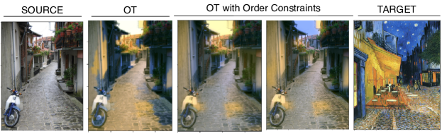
Figure 1: Color transfer using OT with Order Constraints

The order constraints allow context to be taken into account, explicitly, when known in advance, or implicitly, when estimated through the proposed procedure. Consider OT for document retrieval (e.g., see Kusner et al. (2015); Swanson et al. (2020)) where a user enters a text query. The multiple transport plans provided by OT with order constraints offer a diverse set of the best responses, each accounting for different possible contexts. The resulting method is weakly-supervised with only two tunable thresholds (or unsupervised if the parameters are set to default values), and is amenable to applications of OT where labels are not available to train a supervised model.

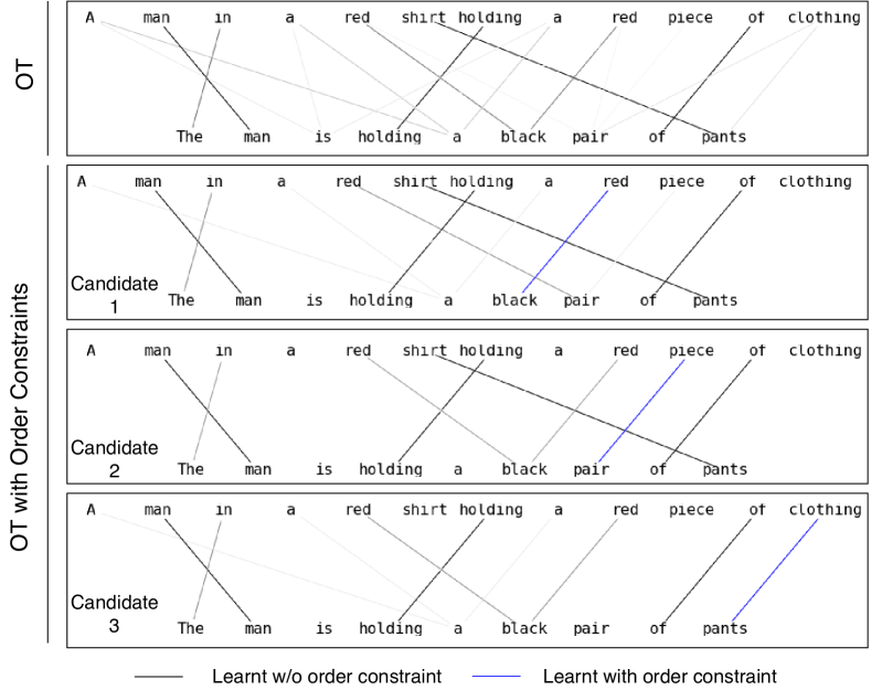
Figure 2: Text matching using OT with Order Constraints

An example is provided in Fig. 2 which aims to learn the similarity between two phrases. The top box depicts the transport plan learnt by OT; the darker the line, the stronger the transport measure. The match provided by OT does not reveal the contradiction in the two phrases. The second to fourth transport plans are more human-interpretable. The second plan matches “red” clothing to the “black” pants. The third matches “piece” to “pair”, a relation not included in the standard OT plan. The last plan matches “clothing” to “pants”. The example makes use of OT with a single order constraint to better illustrate the idea of order constraints. OT with multiple order constraints can incorporate all of the pairs in a single plan.

Fig. 1 illustrates using OT to transfer the color palette of a target image (Van Gogh’s ”Café Terrace at Night”) to the source image of an alley. The second image from the left, obtained by standard OT, transfers yellow to bright areas and blue to dark. Our proposed order constraints allow adding context, which in this case gives desired effects such as transferring the Van Gogh night sky (second image from right) or the awning brilliant yellow (middle image) to the sky in the source image.

The contributions of this work are as follows: (1) we provide a novel formulation, Optimal Transport with Order Constraints, that allows explicitly incorporating structure to OT plans; (2) we provide an efficient method for solving the proposed OT with OC formulation related to an ADMM along with the convergence theory; (3) for cases where the order constraints are not known in advance, we propose an explainable method to estimate them using branch & bound and define bounds for use in the method, and (4) we demonstrate the benefits of using the proposed method on NLP and image color transfer tasks.

Next, we review related work. In the following section, we present the standard optimal transport formulation followed by the proposed OT with order constraints (OT with OC) formulation and a demonstration of the existence of a solution, which corresponds to contribution (1) above. Then, an algorithm leveraging the form of the polytope is defined to solve the OT with OC problem in a manner far more efficient than a standard convex optimization solver, as noted in contribution (2) above. In order to further improve explainability, when the order constraints are not known a priori, we present a branch & bound procedure to search the space for a set of diverse OT with OC plans, along with the bounds that reduce the polynomial search space, as noted in contribution (3) above. Finally, experiments are provided on the e-SNLI dataset and several image color transfer examples to demonstrate how order constraints allow for incorporating structure and improving explainability, as noted in contribution (4) above.

Related Work

We consider point-point linear costs as in e.g., Cuturi (2013); Courty et al. (2017); Kusner et al. (2015); Wu et al. (2018); Yurochkin et al. (2019); Solomon (2018); Altschuler et al. (2019, 2017); Schmitzer (2019). Recently, a number of works have sought to add structure to optimal transport so as to obtain more intuitive and explainable transport plans. Alvarez-Melis et al. (2019) modeled invariances in OT, a form of regularization, to learn the most meaningful transport plan. Sparsity has been explored in OT to implicitly improve explainablity. Swanson et al. (2020) used “dummy” variates to include fewer transport coefficients. Forrow et al. (2019) regularize using the OT rank to better deal with high dimensional data. Blondel et al. (2018) had a similar goal of learning sparse and potentially more intepretable transport plans through regularization and a dual formulation. We, on the other hand, propose an explicit approach to interpretability, rather than the implicit method of sparsifying solutions through regularization. (Su & Hua, 2017) add constraints to require two sequences to lie close to each other, in terms of indices; to respect sequence order, they penalize the constraints and then use the classic Sinkhorn algorithm to obtain an approximate solution. Another way to add structure into OT is through dependency modeling; multi-marginal optimal transport takes this approach, wherein multiple measures are transported to each other. The formulation was shown to be generally intractable (Altschuler & Boix-Adsera, 2020a), however, and strong assumptions have to be made to solve it in polynomial time (Altschuler & Boix-Adsera, 2020b; Pass, 2015; Di Marino et al., 2015).

Standard OT can be solved in cubic time by primal-dual methods (Peyré & Cuturi, 2019) and the proposed OT with order constraints can be solved using generalized solvers with similar time complexity. The difficulty comes from the fact that there are quadratically many order constraints. Recent work (Cuturi, 2013; Scetbon et al., 2021; Altschuler et al., 2017; Goldfeld & Greenewald, 2020; Zhang et al., 2021; Lin et al., 2019; Guo et al., 2020; Jambulapati et al., 2019; Guminov et al., 2021) has favored solving OT via iterative methods which offer lower complexity at the expense of obtaining an approximate solution. In particular, (Scetbon et al., 2021) considered low-rank approximations of OT plans, and proposed a mirror descent with inner Dykstra iterations. Recent iterative methods for standard OT (Guminov et al., 2021; Jambulapati et al., 2019) ensure feasibility of the solution at each iteration through the use of a rounding algorithm proposed by (Altschuler et al., 2017). Iterative methods are essential for solving submodular OT (Alvarez-Melis et al., 2018) that would otherwise incur an exponential number of explicit constraints.

2 Order Constraints for Optimal Transport

Notation

Let $\mathbb{R}$ (resp. $\mathbb{R}_{+}$) denote the set of real (resp. non-negative) numbers. Let $m,n$ denote the number of rows and columns in the optimal transport problem. Vectors and matrices are in $\mathbb{R}^{n}$ and $\mathbb{R}^{m\times n}$. Let $\left[n\right]:=\{1,2\ldots n\}$ and $\left[mn\right]:=\left[m\right]\times\left[n\right]$. Let $i,j,k,\ell,p,q$ denote vector/matrix indices, $2^{\left[n\right]}$ denote the power set of $\left[n\right]$, and $\mathbf{1}_{n}$ and $\mathbf{I}_{n}$ denote the all-ones vector and identity matrix, resp., of size $n$. We denote the index sequence $i_{1},i_{2},\cdots,i_{k}$ as $i_{[k]}$. $\mathbb{I}_{S}($ ) is the indicator function over set $S$. The trace operator for square matrices is denoted by $\mbox{{tr}}\left(\cdot\right)$ and $\mbox{{rank}}\left({X}_{ij}\right)$ gives the descending positions over the $mn$ matrix coefficients ${X}_{ij}$, or a subset thereof. For a closed set $\mathcal{C}$, the Euclidean projector for a matrix $X\in\mathbb{R}^{m\times n}$ is $\mbox{Proj}_{\mathcal{C}}\left(X\right)=\arg\min_{Y\in\mathcal{C}}\left\|Y-X\right\|_{F}^{2}$ where $\left\|\cdot\right\|_{F}$ is the matrix Frobenius norm. For $c\in\mathbb{R}$ let $\left(c\right)_{+}=c$ if $c\geq 0$ and $\left(c\right)_{+}=0$ otherwise, and for $X\in\mathbb{R}^{m\times n}$ let $\left(X\right)_{+}$ equal $X$ after setting all negative coefficients to zero.

Standard OT Formulation

In optimal transport, one optimizes a linear transport cost over a simplex-like polytope, $U(a,b)$. A (balanced) optimal transport problem is given by two probability vectors $a$ and $b$ that each sum to 1. Each being of length $m,n$, resp., they define a polytope:

$$U(a,b)=\{\Pi\in\mathbb{R}^{m\times n}_{+}:\Pi\mathbf{1}_{n}=a,\Pi^{T}\mathbf{1}_{m}=b\},$$

and a linear cost $D\in\mathbb{R}^{m\times n}$, where $D\geq 0$ and bounded. Then the optimal transport cost $f:\mathbb{R}^{m\times n}\to\mathbb{R}_{+}$ is the optimal cost of the following optimization:

$$\min_{\Pi\in U(a,b)}f(\Pi):=\mbox{{tr}}\left(D^{T}\Pi\right),$$ (1)

and the optimal value of $\Pi$ is the transport plan. We propose to extend (1) by including order constraints to represent structure.

Proposed Formulation: OT with Order Constraints

The use of order constraints is analogous to the constraints used in isotonic, or monotonic, regression, (see De Leeuw et al., 2009). Specifically, if a particular variate ${\Pi}_{ij}$ is semantically or symbolically important, then its $\mbox{{rank}}\left({\Pi}_{ij}\right)$ should reflect that dominance. We thus enforce $k$ order constraints by specifying a sequence of $k$ variates in $\left[mn\right]$, $i{j}_{\left[k\right]}:=i_{1}j_{1},i_{2}j_{2},\cdots,i_{k}j_{k}$ of importance, where the set of variates $V:=\left[mn\right]\setminus\{i_{\ell}j_{\ell}:\ell\in\left[k\right]\}$:

$${\Pi}_{i_{k}j_{k}}\geq\cdots\geq{\Pi}_{i_{1}j_{1}}\geq{\Pi}_{pq}~{}~{}\mbox{for}~{}pq\in V.$$ (2)

Enforcing order constraints (2) means each variate $i_{\ell}j_{\ell}$ is fixed to maintain the $(k-\ell+1)$-th top position ${\Pi}_{(k-\ell+1)}$ in the ordering ${\Pi}_{(1)}\geq{\Pi}_{(2)}\geq\cdots\geq{\Pi}_{(mn)}$ whilst learning the transport plan $\Pi$; in particular $i_{k}j_{k}$ is fixed at the topmost position. Therefore, for order constraints on $k$ variates of importance and point-to-point costs $D\in\mathbb{R}^{m\times n}$, we extend the OT problem as follows:

$$\inf_{\Pi\in U(a,b)}f(\Pi):=\mbox{{tr}}\left(D^{T}\Pi\right),$$ (3)

s.t $${\Pi}_{i_{k}j_{k}}\geq\cdots\geq{\Pi}_{i_{1}j_{1}},~{}~{}{\Pi}_{i_{1}j_{1}}\geq{\Pi}_{pq}~{}~{}\mbox{for}~{}pq\in V,$$ (4)

for $V$ in (2), and we assume non-negative costs $D\geq 0$ throughout. Let ${O}_{i{j}_{\left[k\right]}}\subseteq\mathbb{R}^{m\times n}_{+}=$

$$\{X\in\mathbb{R}^{m\times n}_{+}:~{}\mbox{{rank}}\left({X}_{i_{\ell}j_{\ell}}\right)=k-\ell+1,~{}\forall\ell\in\left[k\right]\}.$$ (5)

Thus (3)–(4) can be compactly expressed as:

$$\inf_{\Pi\in U(a,b)\cap{O}_{i{j}_{\left[k\right]}}}f(\Pi).$$ (6)

Problem (6) is convex with linear costs and constraints. However, ${O}_{i{j}_{\left[k\right]}}$ adds a significant number of constraints to the $m+n$ in the standard OT formulation (1). The $\inf$ in (4) and (6) are replaced by $\min$ when feasible; we address such sufficient conditions in the following.

Feasibility of the Proposed OT with OC Problem

$U(a,b)$ is feasible since $ab^{T}\in U(a,b)$, (see Cuturi, 2013). In certain instances it may be considered ambiguous to match a single position to multiple positions, consider variates $i{j}_{\left[k\right]}$ where ${i}_{\left[k\right]}=i_{1},i_{2},\cdots,i_{k}$ (and ${j}_{\left[k\right]}$) do not repeat row (or column) indices; let $\mathbb{I}_{{i}_{\left[k\right]}}(p)=1$ if $p=i_{\ell}$ for at most one choice of $\ell$, or $0$ otherwise, and similarly $\mathbb{I}_{{j}_{\left[k\right]}}(q)$. We next derive conditions for the feasibility of (6) under mild assumptions.

Proposition 2.1.

Suppose ${i}_{\left[k\right]}=i_{1},i_{2},\cdots,i_{k}$ (and ${j}_{\left[k\right]}$) do not repeat row (or column) indices. Further suppose $\Pi\in\mathbb{R}^{m\times n}$, where ${\Pi}_{i_{\ell}j_{\ell}}=c_{\ell}$ for $\ell\in\left[k\right]$, and ${\Pi}_{pq}$ for $pq\in V$, resp. satisfy:

$$0~{}\leq~{}{\Pi}_{i_{\ell}j_{\ell}} = c_{\ell}~{}~{}\leq~{}~{}\min(a_{i_{\ell}},b_{j_{\ell}}),$$ (7)

$$\!\!\!\!\!\!0~{}\leq~{}{\Pi}_{pq}\!\!\! = \!\!\!\frac{(a_{p}-\mathbb{I}_{{i}_{\left[k\right]}}(p)c_{p})\cdot(b_{q}-\mathbb{I}_{{j}_{\left[k\right]}}(q)c_{q})}{\alpha(c_{1},\cdots,c_{\ell})}$$ (8)

where $\alpha=\alpha(c_{1},\cdots,c_{\ell})=1-\sum_{\ell\in\left[k\right]}c_{\ell}\geq 0$. Then, $\Pi$ is feasible w.r.t (6) if:

$$\frac{a_{p}b_{q}}{\alpha(c_{1},\cdots,c_{k})}\leq c_{k}\leq\cdots\leq c_{1}~{}~{}\mbox{for all}~{}~{}pq\in V.$$ (9)

Proof.

Since ${i}_{\left[k\right]}$ and ${j}_{\left[k\right]}$ do not repeat row/column indices, then (7) and (8) imply that $\Pi$ satisfies $\Pi\mathbf{1}_{n}=a$ and $\Pi^{T}\mathbf{1}_{m}=b$; and since they also imply $\Pi\geq 0$, thus $\Pi\in U(a,b)$. Furthermore, we also have $\Pi\in{O}_{i{j}_{\left[k\right]}}$, because (8) and (9) imply for all $pq\in V$, that ${\Pi}_{pq}\leq a_{p}b_{q}/\alpha\leq c_{k}$. ∎

Corollary 2.2.

Suppose ${i}_{\left[k\right]}$ (and ${j}_{\left[k\right]}$) do not repeat row (or column) indices. If $a_{i}=1/m$ and $b_{j}=1/n$, then $\Pi$ is feasible w.r.t (6) if $\min(m,n)\geq(1-k/\max(m,n))^{-1}$.

Proof.

For all $\ell\in\left[k\right]$, pick $c_{\ell}=\min(1/m,1/n)=c$ for some $c\geq 0$; this choice for $c$ satisfies (7) and (8). Then (9) holds if $a_{p}b_{q}/c\leq 1-kc=\alpha$ holds, or equivalently $\min(m,n)\geq(1-k/\max(m,n))^{-1}$ holds. ∎

Cor. 2.2 states for uniform constraints $a_{i}=1/m$ and $b_{j}=1/n$, feasibility typically holds when $k\ll\max(m,n)$, since an upper bound for $(1-k/\max(m,n))^{-1}$ is $1+\mathcal{O}\left(k/\max(m,n)\right)$. Indeed, such is the case of interest where a sparse $k$ number of OCs are enforced, see (2).

3 Solving OT with Order Constraints

In this section we provide a $\delta$-approximate method for (6) that runs in $\mathcal{O}\left(\left\|D\right\|_{\infty}/\delta\cdot mn\log mn\right)$ time using the alternating direction method of multipliers (ADMM) (Boyd et al., 2011; Beck, 2017). In what follows assume feasiblity of (6), and the strategy is to consider the (non-empty) polytope $U(a,b)\cap{O}_{i{j}_{\left[k\right]}}$ as the intersection of two closed convex sets:

$$\mathcal{C}_{1}(a,b) = \{X\in\mathbb{R}^{m\times n}:X\mathbf{1}_{n}=a,X^{T}\mathbf{1}_{n}=b\},$$

and $\mathcal{C}_{2}={O}_{i{j}_{\left[k\right]}}$, used to equivalently rewrite (6) as:

$$\min_{X\in\mathcal{C}_{1}(a,b)}f(X)+\mathbb{I}_{\mathcal{C}_{2}}(Z),$$ (10)

$$\mbox{s.t.}~{}~{}~{}X,Z\in\mathbb{R}^{m\times n},~{}~{}X-Z=\mathbf{0},$$ (11)

where the indicator function $\mathbb{I}_{\mathcal{C}}(X)=0$ if $X\in\mathcal{C}$, and $\mathbb{I}_{\mathcal{C}}(X)=\infty$ otherwise. For $X\in\mathcal{C}_{1}(a,b)$, $Z\in\mathcal{C}_{2}$, the equality implies $X=Z=\Pi$ for feasible $\Pi\in U(a,b)$. The first-order, iterative ADMM procedure is summarized in Algorithm 1; $\rho>0$ is a penalty term, and iterates $X_{t+1},Z_{t+1}$ solve, respectively:

$$\min_{X\in\mathcal{C}_{1}(a,b)}\left(\mbox{{tr}}\left(D^{T}X\right)+\frac{\rho}{2}\left\|X-Z_{t}+M_{t}\right\|_{F}^{2}\right)$$

$$\min_{Z\in\mathbb{R}^{m\times n}}\left(\mathbb{I}_{\mathcal{C}_{2}}(Z)+\frac{\rho}{2}\left\|X_{t+1}-Z+M_{t}\right\|_{F}^{2}\right)$$ (12)

where $M_{t}$ is the (scaled) dual iterate, see (Boyd et al., 2011). Simplifying the first $\min$ expression in (12) shows that $X_{t+1}$ is nothing but the Euclidean projection onto $\mathcal{C}_{1}(a,b)$ of a point $Z_{t}-M_{t}-\rho^{-1}D$; similarly $Z_{t+1}$ is the Euclidean projection onto $\mathcal{C}_{2}$ of $X_{t+1}+M_{t}$.

Algorithm 1 Iterative procedure for OT under OC ${O}_{i{j}_{\left[k\right]}}$ with linear costs $f(X)=\mbox{{tr}}\left(D^{T}X\right)$.

0:  Costs $D$, penalty $\rho$, initial ${M}_{0},{Z}_{0}$.

1:  for round $t\geq 1$ until stopping do

2:     Update $X_{t+1}=\mbox{Proj}_{\mathcal{C}_{1}(a,b)}\left(Z_{t}-M_{t}-\rho^{-1}D\right)$

3:     Update $Z_{t+1}=\mbox{Proj}_{\mathcal{C}_{2}}\left(X_{t+1}+M_{t}\right)$.

4:     Update (scaled) dual variable $M_{t+1}=M_{t}+X_{t}-Z_{t}$.

5:  Return $X_{t}$

We next derive the projections, $\mbox{Proj}_{\mathcal{C}_{1}(a,b)}\left(\cdot\right)$ and $\mbox{Proj}_{\mathcal{C}_{2}}\left(\cdot\right)$, required for Alg. 1. Prop. 3.1 gives the Euclidean projector for $\mathcal{C}_{1}(a,b)$.

Proposition 3.1 (Projection $\mathcal{C}_{1}(a,b)$).

For $\mathcal{C}_{1}(a,b)$ consider the Euclidean projector $\mbox{Proj}_{\mathcal{C}_{1}(a,b)}\left(X\right)$. Let ${P}_{k}$ be the projection of a vector onto its mean, i.e., ${P}_{k}=\frac{1}{k}\mathbf{1}_{k}\mathbf{1}_{k}^{T}$. Define matrices $M:=\mathbf{I}_{m}-\frac{m}{m+n}{P}_{m}$ and $N:=\mathbf{I}_{n}-\frac{n}{m+n}{P}_{n}$, and matrices

$$Y_{1} := \frac{1}{n}\overbrace{\left[Ma,\cdots,Ma\right]^{T}}^{m~{}\mbox{copies (rows)}}+\frac{1}{m}\overbrace{\left[Nb,\cdots,Nb\right]}^{n~{}\mbox{copies (cols)}},~{}~{}~{}~{}~{}$$

$$Y_{2} := M(XP_{n})+(P_{m}X)M.$$ (13)

Then the projection $\hat{X}=\mbox{Proj}_{\mathcal{C}_{1}(a,b)}\left(X\right)$ satisfies $\hat{X}={Y}_{1}+(X-{Y}_{2}).$

The proof of Prop. 3.1 can be found in the Appendix. Wang et al. (2010) proved a similar property for the simplified setting where $a=b=\mathbf{1}_{\cdot}$ and $X$ symmetric, which does not hold in the optimal transport setting.

Next we address computing $\mbox{Proj}_{\mathcal{C}_{2}}\left(X\right)$ for $\mathcal{C}_{2}={O}_{i{j}_{\left[k\right]}}$ for values of $k$ of interest. For the special case where $k=mn$, Grotzinger & Witzgall (1984) defined the so-called Pool Adjacent Violators Algorithm (PAVA) that solves $\mbox{Proj}_{\mathcal{C}_{2}}\left(X\right)$ for $\mathcal{C}_{2}={O}_{i{j}_{\left[mn\right]}}$. We cannot directly make use of PAVA for OT with Order Constraints because we require only a small number, $k\ll mn$, of order constraints, and not the full set, since the OT itself should learn the ordering of the other coefficients.

However, the idea behind PAVA is of interest. To this end we extend PAVA, and call this extension ePAVA. ePAVA projects into $\mathcal{C}_{2}={O}_{i{j}_{\left[k\right]}}$ for general $k$, and is presented in Alg. 2. ePAVA makes use of two quantities defined below; the proof of correctness is given in the Appendix.

We define a block $B$ to be a partition of indices. Let $\texttt{le}[B]$ denote the left and $\texttt{ri}[B]$ the right boundary of $B$; $\texttt{val}[B]$ is the value of its projection. For any $\eta\geq 0$, let $r(\eta)$ denote the $\mbox{{rank}}\left({X}_{i_{1}j_{1}}-\eta\right)$ with respect to decreasing order ${X}_{(1)}\geq{X}_{(2)}\geq\cdots\geq{X}_{(mn-k+1)}$ over all variates in $V\cup\{i_{1}j_{1}\}$, for $V$ in (2). We require averages ${\Delta}_{pq}:=\sum_{\ell=p}^{q}{X}_{i_{\ell}j_{\ell}}/(q-p+1)$ and a threshold function $T(\cdot):=\left(\tau(t(\eta),\eta)\right)_{+}$, where $\tau(s,\eta)$ for any $0\leq s<r(\eta)$ and integer $t(\eta)\geq 0$ are defined as:

$$\tau(s,\eta)\!\! = \!\!\frac{1}{s+1}\left({X}_{i_{1}j_{1}}-\eta+\sum_{\ell=1}^{s}{X}_{(\ell)}\right),$$ (14)

$$t(\eta)+1\!\! = \!\!\arg\min\left\{s\in\left[r\right]:\tau(s,\eta)>X_{(s)}\right\}$$ (15)

or $t(\eta)+1=r(\eta)$ whenever the set in (15) is empty.

Algorithm 2 ePAVA for $\mathcal{C}_{2}={O}_{i{j}_{\left[k\right]}}$ for $k\in\left[mn\right]$

0:  $X\in\mathbb{R}^{m\times n}$. Indices $i{j}_{\left[k\right]}$.

1:  $\ell:=1,B:=1$, $\texttt{le}[1]:=\texttt{ri}[1]:=1$, $\texttt{val}[1]:=T(0)$.

2:  for $\ell\leq k$ do

3:     $B:=B+1$, $\ell:=\ell+1$, $\texttt{le}[B]:=\texttt{ri}[B]:=\ell$, $\texttt{val}[B]:={X}_{i_{\ell}j_{\ell}}$.

4:     for $B\geq 2$ and $\texttt{val}[B]\leq\texttt{val}[B-1]$ do

5:        Let $q=\texttt{ri}[B]$.

6:        if $B=2$ then

7:           Solve and store $\tilde{\eta}\geq 0$ satisfying $T(\tilde{\eta})={\Delta}_{2q}+\tilde{\eta}/(q-1)$. Set $\texttt{val}[B-1]:=T(\tilde{\eta})$.

8:        else

9:           Set $\texttt{val}[B-1]:={\Delta}_{pq}$ for $p=\texttt{ri}[B-1]$.

10:        Set $\texttt{ri}[B-1]:=\texttt{ri}[B]$. Decrement $B:=B-1$.

11:  Return $B,\tilde{\eta}$, le, ri, and val.

Proposition 3.2 (Projection $\mathcal{C}_{2}$).

For $\mathcal{C}_{2}={O}_{i{j}_{\left[k\right]}}$ for any $i_{\ell}j_{\ell}\in\left[mn\right]$ where $\ell\in\left[k\right]$, consider the Euclidean projector $\mbox{Proj}_{\mathcal{C}_{2}}\left(X\right)$ for any $X\in\mathbb{R}^{m\times n}$. Let $T(\eta):=\left(\tau(t(\eta),\eta)\right)_{+}$ for $\tau,t$ in (14) and (15) and $V$ in (2). Then for any $X\in\mathbb{R}^{m\times n}$, ePAVA will successfully terminate with some $B,\tilde{\eta}$, le, ri, and val. Furthermore, the projection $\hat{X}=\mbox{Proj}_{\mathcal{C}_{2}}\left(X\right)$ satisfies i) for $pq\in V$ we have ${\hat{X}}_{pq}=T(\tilde{\eta})=\textup{{val}}[1]$ if $\mbox{{rank}}\left({X}_{pq}\right)\leq t(\tilde{\eta})$ or ${\hat{X}}_{pq}=\left({X}_{pq}\right)_{+}$ otherwise, and ii) for $\ell\in\left[k\right]$ we have ${\hat{X}}_{i_{\ell}j_{\ell}}=\textup{{val}}[B^{\prime}]$ iff $\textup{{le}}[B^{\prime}]\leq\ell\leq\textup{{ri}}[B^{\prime}]$ for some $B^{\prime}\in\left[B\right]$.

Convergence Analysis

Standard ADMM convergence results hold as follows. As $t\rightarrow\infty$, the primal residue $\left\|X_{t}-Z_{t}\right\|_{F}\rightarrow 0$ and dual residue $\rho\left\|Z_{t-1}-Z_{t}\right\|_{F}\rightarrow 0$, which can be used to show asymptotic convergence of $f(X_{t})$ to the optimum (see Boyd, 2010, p. 17). The iteration complexity of Alg. 1 can be obtained from the following non-asymptotic result (see Beck, 2017, Thm 15.4). Consider the following.

As (10)-(11) are both linear, if $\mathcal{C}_{1}(a,b)\cap\mathcal{C}_{2}\neq\emptyset$, then an optimal $Y^{*}=\arg\max_{Y\in\mathbb{R}^{m\times n}}d(Y)$ exists (Boyd & Vandenberghe, 2004) from solving the dual $d(Y):=$

$$\min_{X\in\mathcal{C}_{1}(a,b),Z\in\mathcal{C}_{2}}\mbox{{tr}}\left(X^{T}(D+Y)\right)-\mbox{{tr}}\left(Y^{T}Z\right)$$ (16)

Recall Proposition 2.1 is a sufficient condition for $\mathcal{C}_{1}(a,b)\cap\mathcal{C}_{2}\neq\emptyset$.

Theorem 3.3 (Convergence of Algorithm 1, Beck (2017)).

Let $X_{t},Z_{t},M_{t}$ be the sequences of iterates from Algorithm 1 with penalty $\rho>0$, and let $\bar{X}_{t}=(t+1)^{-1}\sum_{\ell=1}^{t+1}X_{\ell}$ and similarly $\bar{Z}_{t}$. Assume $\mathcal{C}_{1}(a,b)\cap\mathcal{C}_{2}\neq\emptyset$, and let $f^{*}$ and $\Pi^{*}$ denote the optimum value and solution respectively of (6), and $Y^{*}=\arg\max_{Y\in\mathbb{R}^{m\times n}}d(Y)$ for $d(Y)$ in (16). Then we have the convergence bounds

$$f(\bar{X}_{t})-f^{*}\leq\frac{\rho c_{1}}{2(t+1)},~{}~{}~{}\left\|\bar{X}_{t}-\bar{Z}_{t}\right\|_{F}\leq\frac{\rho c_{1}}{c_{2}(t+1)}$$

where $c_{1}\geq\left\|Z_{0}-\Pi^{*}\right\|_{F}^{2}+(\left\|M_{0}\right\|_{F}+c_{2}/\rho)^{2}$ and $c_{2}\geq 2\left\|Y^{*}\right\|_{F}$.

Proposition 3.4 (Iteration complexity).

Algorithm 1, given linear costs $D$ and penalty parameter $\rho\geq 0$, initialized with $Z_{0}=M_{0}=\mathbf{0}$, achieves error $f(\bar{X}_{t})-f^{*}\leq\delta$, in $\mathcal{O}\left(\left\|D\right\|_{\infty}/\delta\right)$ iterations.

Proof.

We seek to estimate $\rho c_{1}$ that bounds the error $f(\bar{X}_{t})-f^{*}$ in Thm. 3.3. First, consider the constant $c_{1}$. Setting $Z_{0}=M_{0}=\mathbf{0}$ gives $\left\|Z_{0}-\Pi^{*}\right\|_{F}^{2}\leq 1$ and $\left\|M_{0}\right\|_{F}=0$, then Thm. 3.3 requires $c_{1}\geq 1+(c_{2}/\rho)^{2}$; hence if we set the penalty $\rho=c_{2}$ then $c_{1}\geq 2$. Next, it remains to estimate $\rho$, or equivalently, $c_{2}$. Thm. 3.3 requires $c_{2}$ to be at least the largest possible norm that an optimizer of the dual (16) can take. To this end if, writing $Y^{*}(D^{\prime})$ for the optimizer of (16) given costs $D^{\prime}$, it suffices to consider a constant $c$ satisfying $c\geq\left\|Y^{*}(D^{\prime})\right\|_{F}$ for any normalized cost $D^{\prime}$ with $\left\|D^{\prime}\right\|_{\infty}=1$, and then picking $c_{2}$ such that $c_{2}\geq 2\left\|D\right\|_{\infty}c$. Hence we arrive at an estimate for $\rho c_{1}$ to be in $\mathcal{O}\left(\left\|D\right\|_{\infty}\right)$. Thus we conclude the error is at most $\delta$ under the claimed number of iterations. ∎

Prop. 3.4 holds for the choice $\rho=c_{2}$, but however $c_{2}$ is unknown in practice; the common adage is to simply set $\rho=1$, (see Boyd et al., 2011). Invoking both Propositions 3.4 and 3.5 below, we estimate the total operation complexity as $\mathcal{O}\left(\left\|D\right\|_{\infty}/\delta\cdot mn\log mn\right)$.

Proposition 3.5.

One round of Algorithm 1 runs in $\mathcal{O}\left(mn\log(mn)\right)$ time.

Proof.

Line 2 costs $\mathcal{O}\left(mn\right)$ for $\mathcal{C}_{1}(a,b)$ and Line 4 costs $\mathcal{O}\left(k+(mn-k)\log(mn-k)\right)$ for $\mathcal{C}_{2}$. The update in Line 2 requires only $\mathcal{O}\left(mn\right)$. Note that for $\mbox{Proj}_{\mathcal{C}_{1}(a,b)}\left(\cdot\right)$ the expressions (13) require only matrix-vector multiplications with $\mathcal{O}\left(mn\right)$ complexity, as follows. For $Y_{1}$ this is clear from (13). For $Y_{2}$, consider the left term $M(XP_{n})$; then the other term $(P_{m}X)M$ similarly follows. Putting $M=\mathbf{I}_{m}-\frac{m}{m+n}{P}_{m}$ and $P_{k}=\frac{1}{k}\mathbf{1}_{k}\mathbf{1}_{k}^{T}$ for $k=m,n$, we get that $M(XP_{n})$ can be expanded (ignoring scaling factors) into two terms $X\mathbf{1}_{n}\mathbf{1}_{m}^{T}$ and $\mathbf{1}_{m}^{T}(\mathbf{1}_{m}X\mathbf{1}_{n})\mathbf{1}_{n}^{T}$. Hence the claim holds given that $\mathbf{1}_{m},\mathbf{1}_{n}$ are vectors.

For $\mathcal{C}_{2}$, observe that computing $T(\eta)=\tau(t(\eta),\eta)$ multiple times in Alg. 2 (Line 7), requires a one-time sort of $mn-k+1$ terms and Lines 5-10 incur an additional $\mathcal{O}\left(k\right)$ following arguments in Grotzinger & Witzgall (1984). ∎

Care should to be taken in comparing our complexity, $\mathcal{O}\left(\left\|D\right\|_{\infty}/\delta\cdot mn\log mn\right)$, to that of OT methods that use rounding approximations Altschuler et al. (2017) to ensure feasibility of each iterate. Such methods, which use KL-divergence, are $\mathcal{O}\left(n^{2}/\delta\cdot\left\|D\right\|_{\infty}\right)$ for $m=n$, (see Guminov et al., 2021; Jambulapati et al., 2019). For order constraints like other structured OT approaches (e.g. Scetbon et al., 2021), a rounding method for $U(a,b)\cap{O}_{i{j}_{\left[k\right]}}$ is not available. However, we have the bound on $\left\|\bar{X}_{t}-\bar{Z}_{t}\right\|_{F}$ in Thm. 3.3 to quantify the feasibility of the iterates $X_{t},Z_{t}$ from $\mathcal{C}_{1}(a,b)\cap\mathcal{C}_{2}$.

4 Explainability via Branch-and-Bound

We have thus far assumed that the structure captured by the optimal transport plan via order constraints has been provided externally. In some settings, the structure is not provided and one must estimate the most important variates to define the corresponding constraints. With the goal of generating plans from which a one can select, we propose an explainable and efficient approach using branch & bound to compute a diverse set of optimal transport plans.

The approach successively computes a bound on the best score that can be obtained with the variates currently fixed; if it cannot improve the best known score, the branch is cut and the next branch, i.e. the next set of fixed variates, is explored. Consider the $k$ order constraints (2) enforced by the variate $i{j}_{\left[k\right]}$, and further consider introducing an additional variate $ij\in\left[mn\right]$ such that ${\Pi}_{i_{k}j_{k}}\geq\cdots\geq{\Pi}_{i_{1}j_{1}}\geq{\Pi}_{ij}\geq{\Pi}_{pq}$ for $pq\in V$, see (2). This manner of introducing variates one-at-a-time, can be likened to variable selection and formalized by a tree structure. On the tree $\mathcal{T}$, each node $i{j}_{\left[k\right]}$ has children $i^{\prime}{j^{\prime}}_{\left[k+1\right]}=ij,i_{1}j_{1},i_{2}j_{2},\cdots,i_{k}j_{k}$ that share the same top-$k$ constraints; the root node corresponds to unconstrained OT, and has children at level $k=1$ corresponding to single order constraint variates $i{j}_{\left[1\right]}=ij$. We would like the procedure to always select all ancestors of a given node before selecting the node itself. Hence, the root node should be selected first.

The branch selection aimed at increasing diversity of the plans is guided by two threshold parameters $\tau_{1},\tau_{2}$ that lie between 0 and 1. For any given node $i{j}_{\left[k\right]}$, the parameters $\tau_{1},\tau_{2}$ limit its children to those that only deliver reasonably likely transport plans, as follows.

Algorithm 3 Learning subtree $\widehat{\mathcal{T}}(k_{1},k_{2},k_{3},\tau_{1},\tau_{2})$ of $\mathcal{T}(k_{3},\tau_{1},\tau_{2})$ and top-$k_{2}$ candidate plans for linear costs $f(\Pi)=\mbox{{tr}}\left(D^{T}\Pi\right)$.

0:  Costs $D$, thresholds $0\leq\tau_{1},\tau_{2}\leq 1$. Search upper limit $k_{1}$, number of top candidates $k_{2}$, and search depth $k_{3}\leq\min(m,n)$.

1:  Compute ${\hat{\Pi}}_{1}$ using (1). Init $\widehat{\mathcal{T}}(k_{1},k_{2},k_{3},\tau_{1},\tau_{2})$.

2:  Use ${\hat{\Pi}}_{1}$, $\tau_{1},\tau_{2}$ in  (17) and (18) to obtain $\mathcal{I}$ and ${\Phi}_{ij}$. Init. $\mathcal{S}=\{(ij,{\Phi}_{ij}):ij\in\mathcal{I}\}$. count=0.

3:  for count $<k_{1}$ do

4:     Pop $i{j}_{\left[k\right]}$ having smallest $\Phi$ in $\mathcal{S}$, for some $k$ constraints. Compute $\mathcal{L}$ from right-hand side of (LABEL:eqn:final-bound).

5:     if ${\hat{\Pi}}_{k_{2}}$ is not yet obtained or $\mathcal{L}>f({\hat{\Pi}}_{k_{2}})$  then

6:        Solve Algorithm 1 with order constraint ${O}_{i{j}_{\left[k\right]}}$ for new candidate $\hat{\Pi}$. Set count += 1.

7:        Update top-$k_{2}$ candidates ${\hat{\Pi}}_{1},{\hat{\Pi}}_{2},\cdots,{\hat{\Pi}}_{k_{2}}$ and $\widehat{\mathcal{T}}(k_{1},k_{2},k_{3},\tau_{1},\tau_{2})$ using new candidate $\hat{\Pi}$.

8:     if $k$ equals $k_{3}$ then

9:        Go to line 4.

10:     if ${\hat{\Pi}}_{k_{2}}$ not yet obtained or $f(\hat{\Pi})<f({\hat{\Pi}}_{k_{2}})$  then

11:        Use $\hat{\Pi}$, $\tau_{1},\tau_{2}$ in  (17) and (18) and obtain new variates $ij\in\mathcal{I}(\hat{\Pi})$ and $\{{\Phi}_{ij}\}_{ij\in\mathcal{I}(\hat{\Pi})}$.

12:        for variate $ij$ in $\mathcal{I}(\hat{\Pi})$ do

13:           if  $i\notin{i}_{\left[k\right]}$ and $j\notin{j}_{\left[k\right]}$  then

14:              Push $(ij,i_{1}j_{1},\cdots,i_{k}j_{k},{\Phi}_{ij})$ onto stack $\mathcal{S}$.

15:  Return top $k_{2}$ candidates ${\hat{\Pi}}_{1},{\hat{\Pi}}_{2},\cdots,{\hat{\Pi}}_{k_{2}}$ and $\widehat{\mathcal{T}}(k_{1},k_{2},k_{3},\tau_{1},\tau_{2})$.

For example, suppose that $\Pi\in U(a,b)$ is the solution of (6) obtained from the variate $i{j}_{\left[k\right]}$. To determine the children of $i{j}_{\left[k\right]}$, first compute saturation levels normalized between $0$ and $1$ given as ${\phi}_{ij}={\Pi}_{ij}/\min(a_{i},b_{j})$, to derive

$$\left({\phi^{s}}_{ij},{\phi^{r}}_{ij},{\phi^{c}}_{ij}\right) = \left({\phi}_{ij},\max_{\ell\in\left[n\right]:~{}\ell\neq i}{\phi}_{i\ell},\max_{\ell\in\left[m\right]:~{}\ell\neq j}{\phi}_{\ell j}\right)$$

$${\Phi}_{ij} := \min({\phi^{r}}_{ij},{\phi^{c}}_{ij}).$$ (17)

Low saturation values in (17) imply uncertainty in the assignments $\Pi$. The thresholds $\tau_{1},\tau_{2}$ are used to determine the set $\mathcal{I}(\Pi)$ that filters those variates $ij$ with low self saturation ($\tau_{1}$) and low neighborhood saturation ($\tau_{2}$):

$$\mathcal{I}(\Pi):=\{ij\in\left[mn\right]:{\phi^{s}}_{ij}\leq\tau_{1},{\Phi}_{ij}\leq\tau_{2}\}.$$ (18)

The children of $i{j}_{\left[k\right]}$ are obtained as $i^{\prime}{j^{\prime}}_{\left[k+1\right]}=ij,i{j}_{\left[k\right]}$ for all $ij\in\mathcal{I}(\Pi)$.

The proposed explainable approach adds diversity by learning the top plans. Let us define $k_{1},k_{2},k_{3}$ as follows: The number of nodes constructed while learning a subtree is at most $k_{1}$, the number of top plans to retain is $k_{2}$, and $k_{3}$, as noted above, limits the tree depth. The branch-and-bound search proceeds on the reduced tree given by $\mathcal{T}(k_{3},\tau_{1},\tau_{2})$, of depth $k_{3}$, containing nodes (18) whose saturation lie beneath the thresholds $\tau_{1},\tau_{2}$. We thus wish to learn the top-$k_{2}$ plans given by subtree, $\widehat{\mathcal{T}}(k_{1},k_{2},k_{3},\tau_{1},\tau_{2})$, and identifying the nodes of $\mathcal{T}(k_{3},\tau_{1},\tau_{2})$ that are in 1-to-1 correspondence with those top-$k_{2}$ plans. The tree $\mathcal{T}(k_{3},\tau_{1},\tau_{2})$ is constructed dynamically, and avoids redundantly computing plans $\Pi$ corresponding to variates $i{j}_{\left[k\right]}$ if the $k_{2}$-best candidate has cost lower than either: i) a known lower bound $\mathcal{L}\leq f(\Pi)$, or ii) the cost of $i{j}_{\left[k\right]}$ parent’s plan. Finally, in the construction of $\mathcal{T}(k_{3},\tau_{1},\tau_{2})$ we conly consider variates where ${i}_{\left[k\right]}$ and ${j}_{\left[k\right]}$ do not repeat indices.

Alg. 3 summarizes the branch-and-bound variable selection procedure. Upon termination, a diverse set of at most $k_{1}$ plans are computed and the $k_{2}$ plans identified by $\widehat{\mathcal{T}}(k_{1},k_{2},k_{3},\tau_{1},\tau_{2})$ are the top-$k_{2}$ amongst these $k_{1}$ plans, as the most uncertain variates are handled first.

Figure 3: Top $k_{2}=5$ candidates for OT with multiple order constraints for the example in Fig. 2

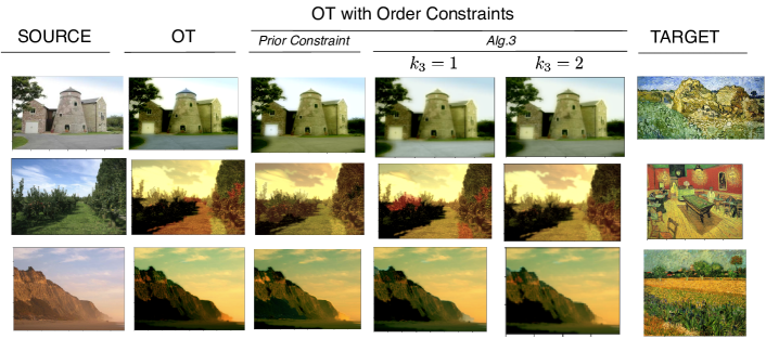
Figure 4: Color transfer candidates obtained using OT with OC (Alg. 3)

It remains to define the lower bound $\mathcal{L}\leq f(\Pi)$ (Line 5); Kusner et al. (2015) proposed a bound for (1), which we extend to the order constrained case (6) as follows:

$$\min_{\Pi\in U(a,b)\cap{O}_{i{j}_{\left[k\right]}}}f(\Pi)\geq$$

$$~{}~{}~{}\min_{\alpha\leq x\leq\beta}\left[{G}_{i{j}_{\left[k\right]}}\cdot x+{g}_{i{j}_{\left[k\right]}}(x,D)\right]$$ (19)

for some suitable $\alpha,\beta$, where $V$ in (2), and where ${G}_{i{j}_{\left[k\right]}}=\sum_{\ell\in\left[k\right]}{D}_{i_{\ell}j_{\ell}},$ and for coefficients $\varphi\in\mathbb{R}^{m\times n}$,

$${g}_{i{j}_{\left[k\right]}}(x,\varphi):=\min_{\Pi\in U(a,b)\cap{O}_{i{j}_{\left[k\right]}}:~{}{\Pi}_{i_{\ell}j_{\ell}}=x,~{}\forall\ell\in\left[k\right]}\sum_{pq\in V}{\Pi}_{pq}{\varphi}_{pq}.$$

We decouple the row and column constraints in (4) and solve $\mbox{{PACKING}}\left(\{{\varphi}_{i}\}_{i\in\left[n\right]},u,\alpha\right)$:

$$\min_{x\in\mathbb{R}^{n}}\sum_{i\in\left[n\right]}{\varphi}_{i}{x}_{i}~{}~{}~{}\mbox{s.t.}~{}~{}~{}~{}\sum_{i\in\left[n\right]}x_{i}=\alpha,~{}~{}~{}0\leq x_{i}\leq u.$$ (20)

Here $u$ and $\alpha$ in (20) represent the per item ${x}_{i}$ capacity and total budget, respectively. Define

$$\mu\left(u,\{\varphi\}_{i\in\left[n\right]},\alpha\right)\!\!\!\!\! = \!\!\!\!\!\mbox{{PACKING}}\left(\{\varphi\}_{i\in\left[n\right]},u,\alpha\right)$$ (21)

$$\nu\left(u,\{\varphi\}_{i\in\left[n-1\right]},\alpha\right)\!\!\!\!\! = \!\!\!\!\!\mbox{{PACKING}}\left(\{\varphi\}_{i\in\left[n-1\right]},u,\alpha-u\right).$$

Proposition 4.1.

Let $\alpha_{1}=\max_{i=1}^{m}\frac{a_{i}}{n},\beta_{1}=\max_{i=1}^{m}a_{i},$, and $\alpha_{2}=\max_{j=1}^{n}\frac{b_{j}}{m},\beta_{2}=\max_{j=1}^{n}b_{j}.$ Then for any $i{j}_{\left[k\right]}$ set enforcing (6) where ${i}_{\left[k\right]}=i_{1},i_{2},\cdots,i_{k}$ (and ${j}_{\left[k\right]}$) do not repeat row (or column) indices, the quantity ${g}_{i{j}_{\left[k\right]}}(x,\varphi)$ appearing in (19) is lower-bounded by

$${g}_{i{j}_{\left[k\right]}}(x,\varphi)\!\!\! \geq \!\!\!\left\{\begin{array}[]{cc}{{L}_{1}}_{ijk}\left(x,\varphi,a\right),&\alpha_{1}\leq x\leq\beta_{1}\\ {{L}_{2}}_{ijk}\left(x,\varphi,b\right),&\alpha_{2}\leq x\leq\beta_{2}\end{array}\right.$$ (24)

where ${{L}_{1}}_{ijk}\left(x,\varphi,a\right)$ and ${{L}_{2}}_{ijk}\left(x,\varphi,b\right)$ equal, resp.

$$\sum_{\ell\in\left[k\right]}\nu\left(x,\{{\varphi}_{i_{\ell}q}\}_{q\in\left[n\right]\setminus\{j_{\ell}\}},a_{i_{\ell}}\right)+\sum_{p\notin{i}_{\left[k\right]}}\mu\left(x,\{{\varphi}_{pq}\}_{q\in\left[n\right]},a_{p}\right)$$

$$\sum_{\ell\in\left[k\right]}\nu\left(x,\{{\varphi}_{pj_{\ell}}\}_{p\in\left[m\right]\setminus\{i_{\ell}\}},b_{j_{\ell}}\right)+\sum_{q\notin{j}_{\left[k\right]}}\mu\left(x,\{{\varphi}_{pq}\}_{p\in\left[m\right]},b_{q}\right)$$

The proof is in the Appendix. Set $\varphi=D$ in (24). Now, from (19) and Prop. 4.1 we obtain:

$$\min_{\Pi\in U(a,b)\cap{O}_{i{j}_{\left[k\right]}}}f(\Pi)$$ (27)

$$\geq \max\left(\begin{array}[]{c}\min_{\alpha_{1}\leq x\leq\beta_{1}}{G}_{i{j}_{\left[k\right]}}\cdot x+{{L}_{1}}_{ijk}\left(x,D,a\right)\\ \min_{\alpha_{2}\leq x\leq\beta_{2}}{G}_{i{j}_{\left[k\right]}}\cdot x+{{L}_{2}}_{ijk}\left(x,D,b\right)\end{array}\right)$$

Thus (LABEL:eqn:final-bound) provides the lower bound in Line 4 of Alg. 3.

5 Experimental Results

Table 1: Task and annotation scores on e-SNLI. BestF1@n is the best achievable annotation F1 score over the set of $k_{2}=$ n best plans, measured by setting coefficients 0 or 1 after determining values under which there is no impact on the the task F1 (75.1 $\pm$ .3). Standard OT achieves 64.5 $\pm$ .3 annotation F1.

Algorithm	BestF1@n
	n$=2$	n$=5$	n$=10$
Algorithm 3 (ours)	68.1 $\pm$ .2	71.2 $\pm$ .3	73.7 $\pm$ .2
Greedy version	67.9 $\pm$ .3	68.2 $\pm$ .3	68.2 $\pm$ .3

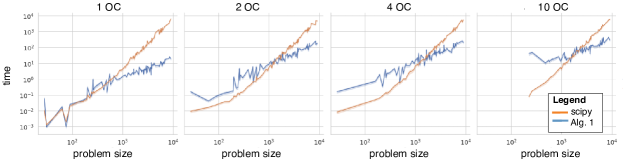
Figure 5: Compute time of Alg. 1 compared with scipy.optimize, for various number of constraints.

Sentence Relationship Classification:

We use an annotated dataset from the enhanced Stanford Natural Language Inference (e-SNLI) (Camburu et al., 2018; Swanson et al., 2020) that includes English sentence pairs classified as “entailment”, “contradiction” or “neutral”. Annotations denote which words were used by humans to determine the class.

We use Alg. 3 to compute $k_{2}$ candidate plans which are measured against the annotations after being set to a binary variable: values above a threshold are set to 1, and below to 0. The threshold is determined as the one that maintains the reported task F1 score when the plan weights that lie below the threshold are set to zero. We determine the $(\tau_{1},\tau_{2})$ that constrain $\mathcal{T}(k_{3},\tau_{1},\tau_{2})$ to be $(\tau_{1},\tau_{2})=(.5,.5)$. Annotations are provided separately on the source and target in each pair; each candidate plan is marginalized using max across columns/rows to arrive at a vector of coefficients, and used to compute an annotation F1 score against the annotations (after application of the threshold). The top $k_{2}=$ n plans are scored using the BestF1@n metric, which reports the score of the best plan in the learnt subtree $\widehat{\mathcal{T}}(k_{1},k_{2},k_{3},\tau_{1},\tau_{2})$. More details can be found in the Appendix.

Table 1 shows the results in terms of the classification task and annotation accuracy along with confidence intervals. Using even only a single order constraint, i.e. $k_{3}=1$, the tree search in Alg. 3 achieves significantly improved explainability using a modest $k_{1}=20$ candidates, giving higher annotation scores over the set of plans. As a baseline against which to compare, we implement a greedy algorithm by restricting the set $\mathcal{I}(\Pi)$ of variates in (18) to contain a single variate, i.e., modifying Lines 2 and 11 of Alg. 3. The greedy algorithm retains the variate $ij\in\mathcal{I}(\Pi)$ with the lowest saturation (17), thus corresponding to a single tree path. For $n\geq 5$, the greedy algorithm results in a candidate set lacking diversity, as evidenced by the stagnating BestF1@n scores as compared to Alg. 3.

Fig. 3 shows the search tree $\mathcal{T}(k_{3},\tau_{1},\tau_{2})$ (blue), the learnt subtree $\widehat{\mathcal{T}}(k_{1},k_{2},k_{3},\tau_{1},\tau_{2})$ (red) and the corresponding candidate plans for the example of Fig. 2 for the top $k_{2}=5$ candidates and depth increased to $k_{3}=3$. See Supp. Mat. for a walk-through of Alg. 3 using Fig. 3 and a study of the effectiveness of the lower bound using a “swarmplot” of # of nodes skipped in the search tree, $\mathcal{T}(k_{3},\tau_{1},\tau_{2})$ as tree depth $k_{3}$ increases. The numbers in Fig. 3 indicate the ranking in the top-$k_{2}$ order upon termination. The diversity provided by Alg. 3 allows the 3rd best solution (in red) to be included in the set of plans, and it is that plan that best explains the contradiction in the two sentences.

Color Transfer

We use source images from the SUN dataset (Xiao et al., 2010; Yu et al., 2016), and target images from WikiArt (Tan et al., 2016). The images are segmented and the average RGB colors in each segment are used to obtain distributions $a,b$ and costs $D$ in the OT formulations (1) and (3). The thresholds that constrain $\mathcal{T}(k_{3},\tau_{1},\tau_{2})$ are set to $(\tau_{1},\tau_{2})=(.5,1.)$ here. Further details on the problem setup can be found in the Appendix.

Results are shown in Fig. 4. The first OT with OC plan includes a prior (human-crafted) constraint while the latter two provide the auto-generated constraints from Alg. 3. The OT with OC solutions offer a range of images, all of which improve upon the standard OT solution in diverse ways. In the first row, standard OT transfers the blue sky to the ground and the cylindrical roof, while the prior constraint maps the green grass from the painting to the ground and intensifies the sky with the blue. The auto-generated constraints from Alg. 3, especially the $k_{3}=2$ case, do the same though slightly less. In the second row, standard OT awkwardly transferred the red to the grass path. The OT with OC solution with a prior constraint as well as the auto-generated constraints of Alg. 3, $k_{3}=2$ use the red to create an evening sky effect. In the third row, standard OT results in a very dark cliff with minimal visible features; the OT with OC solutions lead to a well-defined cliff and more effectively use the blue from the painting sky to deepen the sky in the source image. In addition to producing better resulting images, Alg. 3 allows for human judgement to be used to make the final selection from a set of plans.

Computational Efficiency

Fig. 5 shows how the computation time (in secs) of Alg. 1 scales with problem size. We generate 100 random problems for $m,n\leq 100$ with 1, 2, 4 and 10 order constraints. The iterations are set to terminate at 1e4 rounds or a max projection error of 1e-4, and these settings achieve an average functional approximation of 0.51% error (within $\pm.19$). We use penalty $\rho=1.0$ after testing a range of $\rho$’s and observing little difference, as it is well-known in the ADMM literature (Boyd, 2010). We compare our method against scipy.optimize.

Fig. 5 shows 95% confidence intervals from 10 independent repetitions. Alg. 1 scales much better than scipy.optimize for large problems by orders of magnitude as the problem size $mn$ increases. Note that Fig. 5 compares python-based algorithms; we also evaluated the C++-based cvxpy, and found that our algorithm performs almost indistinguishably to cvxpy for a single order constraint, which is remarkable given the overhead of python as compared to C++.

6 Conclusions

Our proposed optimal transport with order constraints allows complex structure to be incorporated in optimal transport plans and provides a set of explainable solutions from which a human can select. Future extensions of interest are as follows. Other OT solvers may be extended to incorporate order constraints. Such solvers may offer different sets of plans satisfying varying objectives arising from other loss functions and various forms of regularization. See (Flamary et al., 2021). Nonlinear costs such as the submodular formulation of (Alvarez-Melis et al., 2018) can be useful in some settings and may be extended to include order constraints. It would also be of interest to explore other applications that can benefit from OT and specifically OT with OC. Optimal Transport with Order Constraints can be found in the AI Explainability 360 toolbox, which is part of the IBM Research Trusted AI library  (Arya et al., 2019) at https://github.com/Trusted-AI/AIX360.

Appendix

The Appendix comprises two sections. Section A includes further details on the Sentence Relationship Classification and Color Transfer experiments and on the Computational Efficiency of our proposed OT with OC method. Section B of the Appendix includes the proofs for the results in the main paper.

Appendix A Details on Experimental Setup and Results

A.1 Sentence Relationship Classification

For the enhanced Stanford Natural Language Inference (e-SNLI) dataset we follow Swanson et al. (2020) to evaluate explainablity of an OT scheme, whereby annotation-based scores are measured after applying a threshold to determine the activations. The threshold is taken as the one that balances task and explainabilty performance; it should be a sufficiently high so that we do not get spurious activations, and sufficiently low so that enough coefficients are preserved to not compromise the task scores. e-SNLI provides annotation labels to determine the explainability performance, quantified by the annotation F1. The highest annotation F1 score over n $=k_{2}$ candidates of the Algorithm 3 determines the BestF1@n scores. The Greedy version used as a baseline is scored the same way. We used sizes of (100K, 10K, 5K) for train, validation, and test, respectively.

Picking the threshold for the classification task:

This is a three class “entailment”, “neutral” and “contradiction” classification task to predict logical relationships between sentence pairs. The task is performed by a shallow neural network that incorporates an OT attention module between the input and output layers layers. The attention layer uses OT to match source and target tokens, and matched tokens are concatenated and output via softmax. The shallow network is trained on the un-thresholded plan. Over the validation and tests sets, all coefficients that lie below $T/(mn)$ are dropped when measuring the task F1. Using the validation set, we pick the threshold in the region between $0.01$ and $2$ where the task F1 starts to plateau due to the dropped coefficients; we use an activation threshold of $2$.

Comparing activations with annotation labels:

In e-SNLI, annotations that are provided separately on the source and target sentence. Swanson et al. (2020) proposed to marginalize the transport plan $\Pi\in U(a,b)$ forming two vectors for comparison, by applying max to each row and column; we found that this method overlooks the coupling in the transport plan $\Pi$, and we propose instead taking $\max$ only over row/column positions that have annotations labels. On the other hand we cannot then utilize “neutral” examples for measuring annotation F1 (since these examples are missing row annotations), but we do not consider this as a drawback of our proposal because Camburu et al. (2018) indicated that the annotations for the “neutral” examples are curated in a somewhat inconsistent manner from the other example classes, and we thus omit them from the annotation scores.

Hyperparameters:

Alg. 3 takes a standard OT baseline $\Pi\in U(a,b)$ to generate the variate set $\mathcal{I}(\Pi)$, see (18). We use a regularized OT (the hyper-parameter-less mirror descent version of standard OT (see Scetbon et al., 2021) with 20 iterations) to obtain $\Pi$. The standard OT solution lies on a polytope and has at most $m+n$ non-zeros out of the $mn$ locations (Peyré & Cuturi, 2019). The regularized version produces more non-zeros that give more information for seeking unsaturated locations in (18). For the standard OT attention network we do the same with a lower 5 iterations to speed up training.

We obtain $(\tau_{1},\tau_{2})$ that constrain $\mathcal{T}(k_{3},\tau_{1},\tau_{2})$, as follows. First compute transport plans $\Pi\in U(a,b)$ by solving (1), using the regularized version see above, and computing $\phi_{ij}^{s}$ and $\Phi_{ij}$ using (18). The polytope $U(a,b)$ constrains the points $(\phi_{ij}^{s},\Phi_{ij})$ to lie in a lower triangular region bounded by the horizontal and vertical axes and a line that runs through $(1,0)$ and $(0,1)$. The plan coefficients that are uncertain will lie in a box region bounded by the axes $\tau_{1}$ and $\tau_{2}$. Using SNLI annotations as labels that indicate importance, we chose $(\tau_{1},\tau_{2})=(.5,.5)$. We only consider variates $ij$ in (18) if both $i,j$ do not correspond to stop-words. The transport plan is marginalized using max across columns/rows to arrive at a vector of coefficients, and we compute an annotation F1 score against the annotations. The top $k_{2}=$ n plans are scored using the BestF1@n metric, which reports the score of the best plan in the learnt subtree $\widehat{\mathcal{T}}(k_{1},k_{2},k_{3},\tau_{1},\tau_{2})$.

Walkthrough of Alg. 3 using Fig. 3:

At Line 1, the root node (labeled R) and its candidate plan $\hat{\Pi}_{1}$ are computed, and $\widehat{\mathcal{T}}(k_{1},k_{2},k_{3},\tau_{1},\tau_{2})$ is initialized. At Line 2 the single order constraint nodes are constructed and pushed to stack $\mathcal{S}$ along with saturations ${\Phi}_{ij}$ using  (17). At Line 4 a variate $ij$ corresponding to a single order constraint (e.g., “piece”-“pair”) is popped off, and at Line 6 a new candidate $\hat{\Pi}_{2}$ is computed. At Line 7 this candidate is identified by adding $ij$ to $\widehat{\mathcal{T}}(k_{1},k_{2},k_{3},\tau_{1},\tau_{2})$ which now has two nodes. Then at Lines 11-14, new depth-2 nodes $i{j}_{\left[2\right]}=i^{\prime}j^{\prime}ij$ are computed from $\hat{\Pi}_{2}$ and pushed to $\mathcal{S}$ to be considered next in $\mathcal{T}(k_{3},\tau_{1},\tau_{2})$ (e.g., “piece”-“pair” followed by “clothing”-“pants”). Lines 3-14 iterate to update $\widehat{\mathcal{T}}(k_{1},k_{2},k_{3},\tau_{1},\tau_{2})$ and the candidate set. Once $\widehat{\mathcal{T}}(k_{1},k_{2},k_{3},\tau_{1},\tau_{2})$ grows to $k_{2}$ nodes, the lower bound test at Lines 5 and 11 prune redundant nodes of $\mathcal{T}(k_{3},\tau_{1},\tau_{2})$. The iterations terminate when count reaches $k_{1}$.

Hardware and compute times:

Classifier training was performed on a multi-core Ubuntu virtual machine and on a nVidia Tesla P100-PCIE-16GB GPUs. For the shallow neural nets GPU memory consumption was found $<$ 1GB. Training times for 10 epochs (around 5 million sample runs) were roughly 21 hours. Algorithm 3 took about 16 hours to complete over the test set.

A.2 Color Transfer

For the source image, we use Felzenszwalb & Huttenlocher (2004) to preserve pixel locality (see Alvarez-Melis et al., 2018), and for the target we perform color RGB segmentation via $k$-means, in the range of 5-10 color clusters. We illustrate the results of Alg. 3 on three examples from learnt subtrees $\widehat{\mathcal{T}}(20,5,1,\tau_{1},\tau_{2})$ and $\widehat{\mathcal{T}}(40,10,2,\tau_{1},\tau_{2})$, where in this set of experiments we chose $(\tau_{1},\tau_{2})=(0.5,1.0)$. Here we have no labels to tune $(\tau_{1},\tau_{2})$ as we did for e-SNLI. The neighbour saturation metric ${\Phi}_{ij}$ (see (17)) had less effect in this application. Therefore, it sufficed here to use non-regularized OT to compute the base-plan $\Pi\in U(a,b)$. We use the 5 largest source image segments and the 2 largest target image segments in terms of $D_{ij}$; that is, we only consider source image segments large enough to be visually significant, and target image segments with contrasting colors. The WikiArt dataset can be found at https://github.com/cs-chan/ArtGAN/tree/master/WikiArt%20Dataset.

A.3 Computational Efficiencies

Computation Issues

Each computation run of Alg. 1 is measured on a single Intel x86 64 bit Xeon 2MHZ with 12GB memory per core. Also, since the python library scipy.optimize depends on numpy and can run numpy with multiple threads, for fair comparison with our (single-threaded) implementation of Alg. 1, we disabled all parallelisms.

Effectiveness of Lower Bound (LABEL:eqn:final-bound) in Alg. 3

Figure 6 demonstrates the effectives of the lower bound (LABEL:eqn:final-bound), by showing the number of search tree nodes in $\mathcal{T}(k_{3},\tau_{1},\tau_{2})$ that were skipped while performing the e-SNLI experiment for various depths $k_{3}=1,2,3$ and a large candidate size $k_{1}=40$. The bounds show to be effective in skipping more nodes as the size of $\mathcal{T}(k_{3},\tau_{1},\tau_{2})$ increases with the depth $k_{3}$.

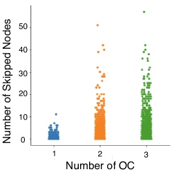
Figure 6: Effectiveness of lower bound (LABEL:eqn:final-bound) in terms of nodes skipped in $\mathcal{T}(k_{3},\tau_{1},\tau_{2})$ for various depths $k_{3}=1,2,3$.

Appendix B Proofs

First we provide the proofs of the propositions concerning the projections, Proposition 3.2 and Proposition 3.1. Secondly, we cover the bounds, giving the proof of correctness of Proposition 4.1.

B.1 Projections

The projection $\mbox{Proj}_{\mathcal{C}_{2}\cap\mathcal{C}_{2}}\left(X\right)=\arg\min_{Y\in\mathcal{C}_{2}}\left\|Y-X\right\|_{F}^{2}$ involves $mn-k$ constraints ${Y}_{pq}\leq{Y}_{i_{1}j_{1}}$ for $pq\in V$ where $V$ in (2), followed by $mn-k+1$ constraints $0\leq{Y}_{pq}$ for $pq\in V\cup\{i_{1}j_{1}\}$, and $k-1$ constraints ${Y}_{i_{\ell}j_{\ell}}\leq{Y}_{i_{\ell+1}j_{\ell+1}}$ for $\ell\in\left[k-1\right]$. Write ${\lambda}_{pq},{\delta}_{pq}$ and $\eta_{\ell}$ for their respective Lagrangian variables and the Karush-Kuhn-Tucker (KKT) conditions:

$${Y}_{pq} = \left\{\begin{array}[]{lll}{X}_{pq}-{\lambda}_{pq}+{\delta}_{pq}&\mbox{for all}&pq\in V\\ {X}_{i_{1}j_{1}}-\eta_{1}+\sum_{pq\in V}{\lambda}_{pq}+{\delta}_{i_{1}j_{1}}&\mbox{for}&pq=i_{1}j_{1}\\ {X}_{i_{\ell}j_{\ell}}+\eta_{\ell-1}-\eta_{\ell}&\mbox{for all}&pq=i_{\ell}j_{\ell}~{}~{}\mbox{where}~{}~{}2\leq\ell\leq k\end{array}\right.$$ (32)

$${Y}_{pq} \leq {Y}_{i_{1}j_{1}},~{}~{}~{}\mbox{for all}~{}~{}~{}pq\in V,~{}~{}\mbox{and}~{}~{}~{}~{}{Y}_{pq}\geq 0~{}~{}~{}~{}~{}~{}~{}~{}~{}\mbox{for all}~{}~{}~{}pq\in V\cup\{i_{1}j_{1}\}$$ (33)

$${\lambda}_{pq} \geq 0,~{}~{}~{}\mbox{for all}~{}~{}~{}pq\in V,~{}~{}~{}~{}~{}~{}~{}~{}\mbox{and}~{}~{}~{}~{}{\delta}_{pq}\geq 0~{}~{}~{}~{}~{}~{}~{}~{}~{}~{}\mbox{for all}~{}~{}~{}pq\in V\cup\{i_{1}j_{1}\}$$ (34)

$${\lambda}_{pq}({Y}_{pq}-{Y}_{i_{1}j_{1}}) = 0,~{}~{}~{}\mbox{for all}~{}~{}~{}pq\in V,~{}~{}~{}~{}~{}~{}~{}~{}\mbox{and}~{}~{}~{}~{}{\delta}_{pq}{Y}_{pq}=0~{}~{}~{}~{}\mbox{for all}~{}~{}~{}pq\in V\cup\{i_{1}j_{1}\}$$ (35)

$${Y}_{i_{\ell}j_{\ell}} \leq {Y}_{i_{\ell+1}j_{\ell+1}},~{}~{}~{}\mbox{for all}~{}~{}~{}\ell\in\left[k-1\right]$$ (36)

$$\eta_{\ell} \geq 0,~{}~{}~{}\mbox{for all}~{}~{}~{}\ell\in\left[k-1\right]$$ (37)

$$\eta_{\ell}({Y}_{i_{\ell+1}j_{\ell+1}}-{Y}_{i_{\ell}j_{\ell}}) = 0,~{}~{}~{}\mbox{for all}~{}~{}~{}\ell\in\left[k-1\right]$$ (38)

Lemma B.1.

Given any index $ij=i_{1}j_{1}$ and positive $\eta\geq 0$, any ${X}_{pq}\in\mathbb{R}$ for all $pq\in V\cup\{ij\}$, let $r=r(\eta)=\mbox{{rank}}\left({X}_{ij}-\eta\right)$ over the $mn-k+1$ variates. Then for both $\tau(\cdot)=\tau(\cdot,\eta)$ and $0\leq t=t(\eta)<r$ (see both (14) and (15) in main text) we have

$$\tau(t,\eta)\geq{X}_{(t+1)},~{}~{}\mbox{and if}~{}~{}t>0~{}~{}\mbox{also}~{}~{}\tau(t,\eta)\leq{X}_{(t)}\leq{X}_{(t-1)}\leq\cdots\leq{X}_{(1)}.$$ (39)

Proof of Lemma B.1.

Assume $\eta=0$ and drop $\eta$ from $\tau$ and $t$, since the case $\eta>0$ is equivalent to the case ${X^{\prime}}_{pq}={X}_{pq}$ and ${X^{\prime}}_{ij}={X}_{ij}-\eta$. Then, the statement (39) holds if (i) ${X}_{(t)}\geq\tau(t)$ and (ii) $\tau(t)\geq{X}_{(t+1)}$. Fact (i) is relevant only when $t>0$, and holds by definition (see (15) in main text) because $t+1$ is minimal in $\left[r\right]$ for which $\tau(t+1)>{X}_{(t+1)}$ holds. Fact (ii) holds in either of the possible two cases:

Case I: [$t+1=r$]. In this case, note $\tau(t)$ is in fact the unweighted average of ${X}_{(t+1)}={X}_{ij}$ and values ${X}_{pq}$ that have higher $\mbox{{rank}}\left({X}_{pq}\right)>r$. Therefore we must conclude $\tau(t)\geq{X}_{(t+1)}$.

Case II: [$t+1<r$]. In this case, note that by definition of $t$ we must have $\tau(t+1)>{X}_{(t+1)}$ is satisfied. Together with $(t+1)\cdot\tau(t+1)=t\cdot\tau(t)+{X}_{(t+1)}$ we have $\tau(t)>\tau(t+1)$. Therefore we conclude $\tau(t)>\tau(t+1)>{X}_{(t+1)}$. ∎

Lemma B.2.

Given any index $ij=i_{1}j_{1}$ and positive $\eta\geq 0$, any ${X}_{pq}\in\mathbb{R}$ for all $pq\in V\cup\{ij\}$, for where at least one $X_{pq}$ in $V\cup\{ij\}$ is negative. Let $1\leq s\leq t$ denote the least-ranked element that is negative in the ranking ${X}_{(1)}\geq\cdots\geq{X}_{(s-1)}\geq 0>{X}_{(s-1)}\geq\cdots\geq{X}_{(t)}$ for $t=t(\eta)$ satisfying (15) in main text. Then for $\tau(\cdot)=\tau(\cdot,\eta)$ in (14), if $\tau(t)<0$, we necessarily have:

$${X}_{ij}<0,~{}~{}\mbox{and}~{}~{}\sum_{\ell=1}^{s-1}{X}_{(\ell)}<-{X}_{ij},$$ (40)

Proof of Lemma B.2.

Assume $\eta=0$ and drop $\eta$ from $\tau$ and $t$, since the case $\eta>0$ is equivalent to the case ${X^{\prime}}_{pq}={X}_{pq}$ and ${X^{\prime}}_{ij}={X}_{ij}-\eta$. We get that $\tau(s)=(s+1)^{-1}\cdot(\sum_{\ell=1}^{s-1}{X}_{(\ell)}+{X}_{(s)}.+{X}_{ij})\leq{X}_{(s)}$, where the inequality follows from the minimality of $t$ in (15). Re-arranging, we get $\sum_{\ell=1}^{s-1}{X}_{(\ell)}+{X}_{ij}\leq{X}_{(s)}$. On the other hand, we had assumed ${X}_{(s)}<0$, so therefore we must conclude (40). ∎

Lemma B.3.

Given index $ij=i_{1}j_{1}$ and $\eta\geq 0$, coefficients ${X}_{pq}\in\mathbb{R}$ for all $pq\in V\cup\{ij\}$, let $r=r(\eta)=\mbox{{rank}}\left({X}_{ij}-\eta\right)$ over the $mn-k+1$ coefficients. Let $\tau(\cdot)=\tau(\cdot,\eta)$ and $0\leq t=t(\eta)$ respectively satisfy (14) and (15) in the main text. For all $pq\in V\cup\{ij\}$, set ${Y}_{pq}$ as: i) if $\mbox{{rank}}\left({X}_{pq}\right)\leq t$ or $pq=ij$ then set ${Y}_{pq}=\left(\tau(t,\eta)\right)_{+}$, and ii) if otherwise then set ${Y}_{pq}=\left({X}_{pq}\right)_{+}$. Then the $mn-k$ and $mn-k+1$ coefficients ${\lambda}_{pq}$ and ${\delta}_{pq}$ as determined by the first two lines of (32), given this choice for ${Y}_{pq}$ and ${X}_{pq}$, satisfy (33)–(35) together with the chosen ${Y}_{pq}$ and ${X}_{pq}$.

Proof of Lemma B.3.

Fix any $ij=i_{1}j_{1}$. Assume $\eta=0$, because the general case $\eta\geq 0$ is equivalent to the case ${X^{\prime}}_{pq}={X}_{pq}$ and ${X^{\prime}}_{ij}={X}_{ij}-\eta$, hence we simply write $\tau(\cdot)=\tau(\cdot,\eta)$ and $t=t(\eta)$. We show that (43)-(44) below

$$(\mbox{for all}~{}pq\in V)~{}~{}~{}~{}~{}~{}~{}~{}~{}~{}~{}~{}~{}~{}~{}~{}~{}{Y}_{pq} = \left\{\begin{array}[]{cc}\left(\tau(t)\right)_{+}&\mbox{if}~{}\mbox{{rank}}\left({X}_{pq}\right)\leq t\\ \left({X}_{pq}\right)_{+}&\mbox{otherwise}\end{array}\right.$$ (43)

$${Y}_{ij} = \left(\tau(t)\right)_{+},$$ (44)

together with (39) and (40) in Lemmatta B.1 and B.2 respectively, establish ${\lambda}_{pq}$ and ${\delta}_{pq}$ that relate ${Y}_{pq}$ and ${X}_{pq}$ by (the first two equations of) (32), and satisfy the three KKT conditions (33), (34) and (35) for $i_{i}j_{1}=ij$, proving the lemma.

KKT condition (33). We first show ${Y}_{pq}\leq{Y}_{ij}$ for all $pq\in V$. Consider $\mbox{{rank}}\left({X}_{pq}\right)>t$. Then wherever ${X}_{pq}\geq 0$ we have $0\leq{Y}_{pq}\stackrel{{\scriptstyle\eqref{order:eqn:condition-C1}}}{{=}}{X}_{pq}\leq{X}_{(t+1)}\stackrel{{\scriptstyle\eqref{order:eqn:condition-A}}}{{\leq}}\tau(t)\stackrel{{\scriptstyle\eqref{order:eqn:condition-C2}}}{{=}}{Y}_{ij}$ , and whenever ${X}_{pq}<0$ we have ${Y}_{pq}\stackrel{{\scriptstyle\eqref{order:eqn:condition-C1}}}{{=}}\left({X}_{pq}\right)_{+}=0\leq\left(\tau(t)\right)_{+}={Y}_{ij}$. For all other $pq\in V$ where $\mbox{{rank}}\left({X}_{pq}\right)\leq t$ we see that ${Y}_{pq}\stackrel{{\scriptstyle\eqref{order:eqn:condition-C1}}}{{=}}\left(\tau(t)\right)_{+}\stackrel{{\scriptstyle\eqref{order:eqn:condition-C2}}}{{=}}{Y}_{ij}$ . Thus the first set of inequalities in (33) follow. The second set ${Y}_{pq}\geq 0$ for all $V\cup\{ij\}$ follow by definitions (43) and (44).

We next show (34) and (35) seperately for $pq\in V$; for $pq\in V$ we choose ${\lambda}_{pq},{\delta}_{pq}$ satisfying ${X}_{pq}+{\delta}_{pq}={\lambda}_{pq}+{Y}_{pq}$ as

$$(\mbox{if}~{}~{}\mbox{{rank}}\left({X}_{pq}\right)>t) \Rightarrow {\lambda}_{pq}=0,~{}~{}\mbox{and}~{}~{}{\delta}_{pq}=\left({X}_{pq}\right)_{+}-{X}_{pq},$$ (45)

$$(\mbox{if}~{}~{}\mbox{{rank}}\left({X}_{pq}\right)\leq t) \Rightarrow \left\{\begin{array}[]{lll}{\lambda}_{pq}={X}_{pq}-\left(\tau(t)\right)_{+},&{\delta}_{pq}=0,&\mbox{if}~{}\tau(t)\geq 0~{}\mbox{or}~{}{X}_{pq}\geq 0,\\ {\lambda}_{pq}=0,&{\delta}_{pq}=-{X}_{pq},&\mbox{if}~{}\tau(t)<0~{}\mbox{and}~{}{X}_{pq}<0\end{array}\right.$$ (48)

Verify (45) satisfies (first equation of) (32) by putting ${Y}_{pq}=\left({X}_{pq}\right)_{+}$ as in (43), and similarly verify (48) satisfies the same by putting ${Y}_{pq}=\left(\tau(t)\right)_{+}$ whilst considering both cases $\tau(t)\geq 0$ and $\tau(t)<0$. Following that (34) and (35) for the remaining index $ij$ will be shown after.

KKT condition (34) for $pq\in V$. Consider $\mbox{{rank}}\left({X}_{pq}\right)>t$. From (45), this is trivally satisfied for ${\lambda}_{pq}$, and holds for ${\delta}_{pq}$ because $\left({X}_{pq}\right)_{+}-{X}_{pq}\geq 0$. For $\mbox{{rank}}\left({X}_{pq}\right)\leq t$ we see from (48) the following. We see ${\lambda}_{pq}={X}_{pq}-\left(\tau(t)\right)_{+}\geq 0$ holds in the event where either $\tau(t)\geq 0$ or ${X}_{pq}\geq 0$ holds, since $\tau(t)\stackrel{{\scriptstyle\eqref{order:eqn:condition-A}}}{{\leq}}{X}_{pq}$ whenever $\mbox{{rank}}\left({X}_{pq}\right)\leq t$. Also in the event where both $\tau(t)<0$ and $X_{pq}<0$ hold, we have that $\delta_{pq}=-{X}_{pq}\geq 0$ because then we have ${X}_{pq}$ to be negative.

KKT condition (35) for $pq\in V$. The first set of equalities in (35) satisfy as follows. Whenever $\mbox{{rank}}\left({X}_{pq}\right)\leq t$, we have ${Y}_{pq}={Y}_{ij},$ see above discussion on KKT condition (33). For $\mbox{{rank}}\left({X}_{pq}\right)>t$, we had chosen ${\lambda}_{pq}=0$, see (45). The second set of equalities in (35) satisfy as follows: for case $\mbox{{rank}}\left({X}_{pq}\right)>t$ this is seen given choice (43) putting ${Y}_{pq}=\left({X}_{pq}\right)_{+}$ and choice (45) for ${\delta}_{pq}$, and for $\mbox{{rank}}\left({X}_{pq}\right)\leq t$ this is seen given (43) putting ${Y}_{pq}=\left(\tau(t)\right)_{+}$ and choice (48) for ${\delta}_{pq}$.

It remains to show KKT conditions ${\delta}_{ij}\geq 0$ in (34) and ${\delta}_{ij}{Y}_{ij}=0$ in (35). Derive the following:

$$\sum_{pq\in V}{\lambda}_{pq}\stackrel{{\scriptstyle\eqref{order:eqn:condition-E}}}{{=}}\sum_{pq\in V:~{}\mbox{{rank}}\left({X}_{pq}\right)\leq t}({X}_{pq}+{\delta}_{pq}-\left(\tau(t)\right)_{+})~{}~{}~{}~{}=~{}~{}~{}~{}\sum_{pq\in V:~{}\mbox{{rank}}\left({X}_{pq}\right)\leq t}\left({X}_{pq}+{\delta}_{pq}\right)-t\cdot\left(\tau(t)\right)_{+}.$$

Then put ${Y}_{ij}=\left(\tau(t)\right)_{+}$ from (44) in ${\delta}_{ij}={Y}_{ij}-{X}_{ij}-\sum_{pq\in V}{\lambda}_{ij}$, and put in the derivation above to get ${\delta}_{ij}=(t+1)\cdot\left(\tau(t)\right)_{+}-({X}_{ij}+\sum_{pq\in V:~{}\mbox{{rank}}\left({X}_{pq}\right)\leq t}({X}_{pq}+{\delta}_{pq}))$, and simplify to:

$${\delta}_{ij} = \left\{\begin{array}[]{ll}(t+1)\tau(t)-({X}_{ij}+\sum_{pq\in V:~{}\mbox{{rank}}\left({X}_{pq}\right)\leq t}{X}_{pq})\stackrel{{\scriptstyle\eqref{eqn:order-threshold-tau}}}{{=}}(t+1)\tau(t)-(t+1)\tau(t)=0&\mbox{if}~{}\tau(t)\geq 0\\ -{X}_{ij}-\sum_{pq\in V:~{}\mbox{{rank}}\left({X}_{pq}\right)\leq t}({X}_{pq}+{\delta}_{pq})\stackrel{{\scriptstyle\eqref{order:eqn:condition-D}}}{{=}}-{X}_{ij}-\sum_{pq\in V:~{}{X}_{pq}\geq 0}{X}_{pq}\stackrel{{\scriptstyle\eqref{order:eqn:condition-A2}}}{{>}}0,&\mbox{if}~{}\tau(t)<0\end{array}\right.$$ (51)

showing both (34) and (35) hold, where we had used (40) from Lemma B.2 for the final inequality in the $\tau(t)<0$ case. ∎

Lemma B.4.

For $\tau(\cdot,\eta)$ and $t(\eta)$ in (14) and (15) in the main text, consider the function $T:\mathbb{R}_{+}\mapsto\mathbb{R}$ defined as $T(\eta):=\left(\tau(t(\eta),\eta)\right)_{+}$ for any $\eta\geq 0$. Then $T$ is piecewise-linear, monotonic non-increasing and convex in $\eta\geq 0$.

Proof of Lemma B.4.

$\tau(s,\eta)$ is decreasing linear function of $\eta$ for fixed $s$, therefore $T(\eta)=\left(\tau(t(\eta),\eta)\right)_{+}=\max(\tau(t(\eta),\eta),0)$ is a convex, piecewise linear function with inflection points whenever $t(\eta)$ changes value, with the final inflection point occurring when $\tau(t(\eta),\eta)$ meets the horizontal axis. ∎

Lemma B.5 ((Grotzinger & Witzgall, 1984)).

For $p,q,r,s\in\left[k\right]$ satisfying $1\leq p\leq q\leq r\leq s\leq k$ where $r=q+1$, assume ${\Delta}_{pq}\leq{\Delta}_{sq}$ for $\Delta$ in (52). Let $\ell$ satisfy $p\leq\ell\leq s$. Then for all $\ell\leq q$ we have ${\psi}_{p\ell}-(\ell-p+1){\Delta}_{ps}\geq 0$, and for all $\ell>q$ we have we have ${\psi}_{r\ell}-(\ell-r+1){\Delta}_{rs}\geq 0$.

Restatement of Proposition 3.2

For $\mathcal{C}_{2}={O}_{i{j}_{\left[k\right]}}$ for any $i_{\ell}j_{\ell}\in\left[mn\right]$ where $\ell\in\left[k\right]$, consider the Euclidean projector $\mbox{Proj}_{\mathcal{C}_{2}}\left(X\right)$ for any $X\in\mathbb{R}^{m\times n}$. Let $T(\eta):=\left(\tau(t(\eta),\eta)\right)_{+}$ for $\tau,t$ in (14) and (15) in the main text, and let $V$ in (2). Then for any $X\in\mathbb{R}^{m\times n}$, ePAVA will successfully terminate with some $B,\tilde{\eta}$, le,ri, and val. Furthermore, the projection $\hat{X}=\mbox{Proj}_{\mathcal{C}_{2}}\left(x\right)$ satisfies i) for $pq\in V$ we have ${\hat{X}}_{pq}=T(\tilde{\eta})=\textup{{val}}[1]$ if $\mbox{{rank}}\left({\hat{X}}_{pq}\right)\leq t(\tilde{\eta})$ or ${\hat{X}}_{pq}={X}_{pq}$ otherwise, and ii) for $\ell\in\left[k\right]$ we have ${\hat{X}}_{i_{\ell}j_{\ell}}=\textup{{val}}[B^{\prime}]$ iff $\textup{{le}}[B^{\prime}]\leq\ell\leq\textup{{ri}}[B^{\prime}]$ for some $B^{\prime}\in\left[B\right]$.

Proof.

Proving Proposition 3.2 involves exhibiting a $Y\in\mathbb{R}^{m\times n}$ satisfying (32)–(38). Given variates ${X}_{i_{\ell}j_{\ell}}$ where $i_{\ell}j_{\ell}\notin V$ for all $\ell\in\left[k\right]$, define:

$${\psi}_{pq}=\sum_{\ell=p}^{q}{X}_{i_{\ell}j_{\ell}},~{}~{}~{}{\Delta}_{pq}=\frac{{\psi}_{pq}}{q-p+1},~{}~{}~{}\mbox{for}~{}1\leq p\leq q\leq k.$$ (52)

The block of operations between Lines 4 and 10 of Alg. 2 is termed “coalescing” (Grotzinger & Witzgall, 1984). As coalescing occurs during iterates, in the case whenever $B=2$, notice the parameter denoted $\tilde{\eta}$ in Alg. 2 (Line 7) that updates. We prove that if this parameter is taken to be $\eta_{1}$ in the KKT conditions (32) and (37)–(38), that Alg. 2 terminates and when it does with $\hat{X}$, that $\hat{X}=Y$ satifies the KKT. The proof is recursive in $\eta_{1}$ and we initialize $\eta_{1}=0$. We use $\eta_{\ell}$ and $\eta_{\ell}^{\prime}$ to denote the current, and next iterate, respectively.

We first invoke (32) to fix the relationship between solution and Lagrangian multipliers. For a given $\eta_{1}$ value, put $\eta_{1}=\eta$ in Lemma B.3 to get $mn-k+1$ coefficients ${Y}_{pq}$ (and the Lagrangians ${\lambda}_{pq},{\delta}_{pq}$) for all $pq\in V\cup\{i_{1}j_{1}\}$ satisfying the first two lines of (32) and (33)–(35) of the KKT conditions. Likewise for $\eta_{1}$, we use (32) to derive the $k-1$ Lagrangians that accompany ${Y}_{i_{\ell}j_{\ell}}$ as follows. For any $B^{\prime}\in\left[B\right]$, ePAVA in Alg. 2 sets ${Y}_{i_{\ell}j_{\ell}}={Y}_{i_{\ell+1}j_{\ell+1}}$ for values of $\ell$ that satisfy $\texttt{le}[B^{\prime}]\leq\ell<\ell+1\leq\texttt{ri}[B^{\prime}]$. On the other hand if $\ell$ is on the boundary $\ell=\texttt{ri}[B^{\prime}]$ and $\ell+1=\texttt{le}[B^{\prime}+1]$ then ePAVA results in ${Y}_{i_{\ell}j_{\ell}}\neq{Y}_{i_{\ell+1}j_{\ell+1}}$. Therefore using ${\psi}_{pq}$ and ${\Delta}_{pq}$ from (52) and $\nu=\sum_{pq\in V}{\lambda}_{pq}+{\delta}_{i_{1}j_{1}}$, we express ${Y}_{i_{\ell}j_{\ell}}$ and $\eta_{\ell}$ for all $\ell\in\left[k\right]$:

$$\eta_{\ell} = {\psi}_{1\ell}-\ell\cdot T(\eta_{1})+\nu,~{}~{}~{}~{}~{}{Y}_{i_{\ell}j_{\ell}}=T(\eta_{1}),~{}~{}~{}~{}~{}~{}\mbox{if}~{}~{}1\leq\ell\leq\texttt{ri}[1],$$ (53)

$$\eta_{\ell} = {\psi}_{p\ell}-(\ell-p+1){\Delta}_{pq},~{}~{}~{}{Y}_{i_{\ell}j_{\ell}}={\Delta}_{pq},~{}~{}~{}~{}~{}~{}\mbox{if}~{}~{}p=\texttt{le}[B^{\prime}]\leq\ell\leq q=\texttt{ri}[B^{\prime}]$$ (54)

where (54) is satisfied for all $1<B^{\prime}\leq B$, and simply let $\eta_{k}=0$ since this does not contradict (52). Thus it remains to show, as the iterates of $\eta_{1}$ update the values of ${Y}_{pq},{\lambda}_{pq},{\delta}_{pq},{\eta}_{pq}$ by Lemma B.3 and (53)–(54), the remaining KKT conditions  (36)–(38) are satisfied upon termination of ePAVA. To this end we must prove the existence and required properties of the zero (i.e., $\tilde{\eta}$, taken here to be $\eta_{1}$) in Line 7. Specifically, let $q=\texttt{ri}[1]$ be the boundary of block 1. Suppose either a) $\eta_{1}=0$ and $q=1$, or b) ${\psi}_{2q}-(q-1)\cdot T(\eta_{1})+\eta_{1}=0$ is satisfied for some $\eta_{1}>0$ and $q>1$. Let $r=q+1$ and consider ${\psi}_{2s}$ from (52) for some $s\geq r\geq 2$. We show below that in either case a) or b), that if ${\Delta}_{rs}\leq T(\eta_{1})$ holds, we must have that i) there exists a zero $\eta^{\prime}_{1}$ satisfying ${\psi}_{2s}-(s-1)\cdot T(\eta^{\prime}_{1})+\eta^{\prime}_{1}=0$, and ii) $T(\eta^{\prime}_{1})\leq T(\eta_{1})$ and $\eta^{\prime}_{1}\geq\eta_{1}$.

The proof of the above properties of the zero follow. In the case $\eta_{1}=0$ and $q=1$, then i) follows by equivalently showing if $T(\eta^{\prime}_{1})-\eta^{\prime}_{1}/(s-1)-{\Delta}_{2s}$ has a zero (divide by $(s-1)\geq 1$ and use (52)). Indeed, the zero exists at some $\eta_{1}^{\prime}\geq 0$ since the non-increasing $T(\eta^{\prime}_{1})$, see Lemma B.4, and an increasing linear function $\eta^{\prime}_{1}/(s-1)+{\Delta}_{2s}$, meets, as the latter starts at a point lower than the former as given by the assumption ${\Delta}_{2s}\leq T(0)$. Furthermore, ii) holds since we showed $\eta_{1}^{\prime}\geq 0=\eta_{1}$ and by monotonicity of $T(\cdot)$. In the other case put ${\Delta}_{2s}=(1-\beta){\Delta}_{2q}+\beta{\Delta}_{rs}$ for $0\leq\beta=(s-q)/(s-1)\leq 1$, and use the condition b) above to derive $T(\eta_{1})-{\Delta}_{2s}-\eta_{1}/(s-1)=\beta\cdot(T(\eta_{1})-{\Delta}_{rs})\geq 0$ where the inequality follows since we assumed ${\Delta}_{rs}\leq T(\eta_{1})$. Then by monotonicity of $T(\cdot)$, see Lemma B.4, the zero exists and occurs at some point $\eta_{1}^{\prime}\geq\eta_{1}$ with similar arguments as before showing i) and ii).

KKT condition (37) for block 1, case (53): We now show that for block 1, coalescing recursively maintains non-negativity (37). Suppose $1,q$ and $r,s$ are boundaries of blocks $1$ and $2$, where $\texttt{ri}[1]=q=r-1$. Let $\eta^{\prime}_{\ell}$ for $\ell\in\left[s\right]$ equal (53) after coalescing, rewritten into $\eta^{\prime}_{\ell}={\psi}_{2\ell}-(\ell-1)T(\eta^{\prime}_{1})+\eta^{\prime}_{1}$, and similarly $\eta_{\ell}$ for $\ell\in\left[q\right]$ denotes (53) before coalescing. By recursion assumption either $\eta_{1}=0$ or ${\psi}_{2q}-(q-1)\cdot T(\eta_{1})+\eta_{1}=0$ is satisfied for some $\eta_{1}>0$. ePAVA coalesces blocks 1 and 2 if $\texttt{val}[1]\leq\texttt{val}[2]$, or equivalently, if ${\Delta}_{rs}\leq T(\eta_{1})$ for value $\eta_{1}\geq 0$ , and therefore by recursion assumption, we conclude a new zero $\eta^{\prime}_{1}\geq 0$ of Line 7 with properties i) and ii) above exists. Then for $\ell\leq q$ we have $\eta^{\prime}_{\ell}-\eta_{\ell}=(\ell-1)(T(\eta_{1})-T(\eta_{1}^{\prime}))+\eta^{\prime}_{1}-\eta_{1}$, and by the inequality $\eta^{\prime}_{1}-\eta_{1}\geq 0$, we conclude $\eta^{\prime}_{\ell}-\eta_{\ell}\geq 0$. Next for $\ell>q$, we express the following for some $\alpha=1-(\ell-1)/(s-1)\geq 0$:

$$\eta^{\prime}_{\ell}-\eta_{\ell} \stackrel{{\scriptstyle(a)}}{{=}} \eta^{\prime}_{1}+{\psi}_{2q}-(\ell-1)\cdot T(\eta_{1}^{\prime})+(\ell-q){\Delta}_{rs}\stackrel{{\scriptstyle(b)}}{{=}}\alpha\cdot\left(\eta^{\prime}_{1}+{\psi}_{2q}-(q-1){\Delta}_{rs}\right)$$

$$\stackrel{{\scriptstyle(c)}}{{\geq}} \alpha(q-1)\cdot(T(\eta_{1})-{\Delta}_{rs})\geq 0,$$

where (a) follows from $\eta^{\prime}_{\ell}$ in (53) and $\eta_{\ell}$ in (54), and (b) follows from expressing $T(\eta^{\prime}_{1})=[{\psi}_{2q}+(s-q)\cdot{\Delta}_{rs}+\eta^{\prime}_{1}]/(s-1)$ and collecting terms into $\alpha$, and (c) follows as $\eta^{\prime}_{1}+{\psi}_{2q}\geq\eta_{1}+{\psi}_{2q}=(q-1)\cdot T(\eta_{1}),$ and finally the last inequality follows because we only coalesce when ${\Delta}_{rs}\leq T(\eta_{1})$.

KKT condition (37) for block $>1$, case (54): We show the similar non-negativity property for other blocks. Suppose $p,q$ and $r,s$ are boundaries of two blocks $B^{\prime}$ and $B^{\prime}+1$, where $r=q+1$ and $B^{\prime}>1$. ePAVA coalesces block $B^{\prime}$ and $B^{\prime}+1$ only if $\texttt{val}[B^{\prime}-1]\leq\texttt{val}[B^{\prime}]$, or equivalently, ${\Delta}_{pq}\leq{\Delta}_{rs}$. Consider any $p\leq\ell\leq s$. Eqn. (54) implies that the Lagrangians before and after coalescing are $\eta_{\ell}={\psi}_{p\ell}-(\ell-p+1){\Delta}_{ps}$ and $\eta^{\prime}_{\ell}={\psi}_{r\ell}-(\ell-r+1){\Delta}_{rs}$, respectively. Supposing $\eta_{\ell}\geq 0$ and by these expressions for $\eta^{\prime}_{\ell},\eta_{\ell}$, we thus invoke Lemma B.5 to show $\eta^{\prime}_{\ell}\geq 0$ for all $\ell\leq q$ hold after coalescing; the other case $\ell>q$ also holds similarly by Lemma B.5.

KKT condition (38): We show the coalescing update Lines 4-10, maintains the boundary $s=\texttt{ri}[B^{\prime}]$ for any $B^{\prime}\in\left[B\right]$ property $\eta_{s}=0$; this proves complementary slackness (38) because (53)–(54) shows ${Y}_{i_{\ell}j_{\ell}}$ to differ only across boundaries. Let $\eta_{q}$ and $\eta^{\prime}_{s}$ denote boundary Lagrangians for the previous and current coalescing update, respectively; the boundaries $p,q$ and $r,s$ for $r=q+1$ are coalesced. For (54) for $B^{\prime}>1$, we have for $\eta^{\prime}_{s}={\psi}_{ps}-(s-p+1){\Delta}_{ps}$ at the boundary $\ell=s$, and $\eta_{s}=0$ by definition (52). For (53) for $B^{\prime}=1$, rewrite (53) to get the form $\eta^{\prime}_{s}={\psi}_{2s}-(s-1)\cdot T(\eta^{\prime}_{1})+\eta^{\prime}_{1}$ resembling the equation with the zero shown above. If the coalescing update is executed for the first time, then $\eta_{1}=0$ and $q=1$. Otherwise $\eta_{1}>0$ and $q>1$ and by recursion assumption $\eta_{q}={\psi}_{2q}-(q-1)\cdot T(\eta_{1})+\eta_{1}=0$. Therefore in either cases, together with the condition ${\Delta}_{rs}\leq T(\eta_{1})$ that holds for a coalescing step to occur, we conclude by zero property i) that $\eta^{\prime}_{s}=0$.

KKT condition (36): Each coalescing step of ePAVA attempts to restore a non-increasing property of ${Y}_{i_{\ell}j_{\ell}}$ for all $\ell\in\left[k\right]$. This is only possible if the new values ${Y}_{i_{\ell}j_{\ell}}$ that result from coalescing does not increase beyond the values before coalescing. This is obvious for the case of $B>2$ by definition (52). ePAVA eventually terminates satisfying (36), since there are finite number of coalescsing steps, and in the worst case arrives at the terminating state $B=1$ and $\texttt{ri}[1]=k$ is arrived at, which satisfies (36). ∎

We now turn to the Euclidean projection $\mbox{Proj}_{\mathcal{C}_{1}(a,b)}\left(X\right)$ of a matrix $X\in\mathbb{R}^{m\times n}$ onto the row- and column-sum constraint set $\mathcal{C}_{1}(a,b)$ for measures $a,b$. Let $\otimes$ denote the matrix Kronecker (i.e., tensor) product. Observe that the row-sums of any $X\in\mathbb{R}^{m\times n}$ can also be obtained via Kronecker equivalence $X\mathbf{1}_{n}=(\mathbf{I}_{m}\otimes\mathbf{1}_{n}^{T})x$, where $x\in\mathbb{R}^{mn}$ is a length-$mn$ vector formed from $X\in\mathbb{R}^{m\times n}$ by setting ${x}_{(k-1)n+\ell}={X}_{k\ell}$ . Also be the same equivalence we obtain column-sums of $X\in\mathbb{R}^{m\times n}$ $X^{T}\mathbf{1}_{m}=(\mathbf{1}_{m}\otimes\mathbf{I}_{n})x$ from the same equivalent $x\in\mathbb{R}^{mn}$; in numpy terminology one writes $x=\mbox{ {ravel} }\left(X\right)$. We thus conclude that Euclidean projection $\hat{X}=\mbox{Proj}_{\mathcal{C}_{1}(a,b)}\left(X\right)$ for any $X\in\mathbb{R}^{m\times n}$, can be equivalently obtained by solving the following optimization over $\mathbb{R}^{mn}$:

$$\hat{x}=\arg\min_{y\in\mathbb{R}^{mn}}~{}\frac{1}{2}\left\|y-x\right\|_{2}^{2},~{}~{}\mbox{s.t.}~{}~{}~{}(I_{m}\otimes 1_{n}^{T})y=a,~{}~{}~{}(1_{m}^{T}\otimes I_{n})y=b$$ (55)

and then setting $\hat{X}=\mbox{ {unravel} }\left(\hat{x}\right)$, where $\mbox{ {unravel} }\left(\cdot\right)$ is the operational inverse of numpy function $\mbox{ {ravel} }\left(\cdot\right)$.

Converting the problem to vectors (55) results in KKT conditions with $(m+n)$ (Lagrangian) variables $\alpha\in\mathbb{R}^{m}$ and $\beta\in\mathbb{R}^{n}$ in a system of linear equations:

$$\left[\begin{array}[]{cc}\mathbf{I}_{mn}&A^{T}\\ A&\end{array}\right]\left[\begin{array}[]{c}y\\ \alpha\\ \beta\end{array}\right]=\left[\begin{array}[]{c}x\\ a\\ b\end{array}\right]$$ (64)

where here $A$ is an $(m+n)\times mn$ matrix with first $m$ rows equal $I_{m}\otimes 1_{n}^{T}$ and last $n$ rows equal $1_{m}^{T}\otimes I_{n}$. That is to compute $\hat{X}=\mbox{Proj}_{\mathcal{C}_{1}(a,b)}\left(X\right)$, one may simply solve (64) for $y$, given $x=\mbox{ {ravel} }\left(X\right),a$ and $b$. However we have to pay attention that $A$ in (64) is not full-rank. To compute the exact rank of $A$, we can make use of Remark 3.1 from (Peyré & Cuturi, 2019); specifically, it is $m+n-1$. This implies that the left-inverse of $A$ is not equal to ${(A^{T}A)}^{-1}A^{T}$, and instead requires the pseudo-inverse of the matrix $A\in\mathbb{R}^{(m+n)\times mn}$ in (64):

$${A}^{\dagger}=\left[\begin{array}[]{cc}\frac{1}{n}\left(\mathbf{I}_{m}\otimes\mathbf{1}_{n}-\frac{1}{m+n}\right)&\frac{1}{m}\left(\mathbf{1}_{m}\otimes\mathbf{I}_{n}-\frac{1}{m+n}\right)\end{array}\right].$$

Recall ${P}_{k}$ is the projection ${P}_{k}=\frac{1}{k}\mathbf{1}_{k}\mathbf{1}_{k}^{T}$, and matrices $M:=\mathbf{I}_{m}-\frac{m}{m+n}{P}_{m}$ and $N:=\mathbf{I}_{n}-\frac{n}{m+n}{P}_{n}$. Then (65) will prove Prop. 3.1 , restated here in the Kronecker equivalent form (55) corresponding to numpy function $x=\mbox{ {ravel} }\left(X\right)$.

Lemma B.6.

Assume $a\in\mathbb{R}^{m}$ and $b\in\mathbb{R}^{n}$ have same means, i.e., $a^{T}\mathbf{1}_{n}=b^{T}\mathbf{1}_{n}$. Then for any $x\in\mathbb{R}^{m\times n}$, the solution of (64) is given by the the following expression for $y\in\mathbb{R}^{mn}$ for some $\alpha\in\mathbb{R}^{m}$ and $\beta\in\mathbb{R}^{n}$, where

$$y={A}^{\dagger}\left[\begin{array}[]{c}a\\ b\end{array}\right]+\left(\mathbf{I}_{mn}-A^{T}{\left(A^{T}\right)}^{\dagger}\right)x$$ (65)

where ${A}^{\dagger}$ is the pseudo-inverse of $A\in\mathbb{R}^{(m+n)\times mn}$ in (64).

Proof of Lemma B.6.

Suppose $\left[\begin{array}[]{c}a\\ b\end{array}\right]$ lies in $\mbox{{span}}\left(A\right)$, then our strategy is to show $y\in\mathbb{R}^{mn}$ in (65) satisfies both top (i.e., first $m$ rows) and bottom (i.e., last $n$ rows) of (64), in two steps. From the Moore-Penrose property $A{A}^{\dagger}A=A$ of the pseudo-inverse, we conclude that ${A}^{\dagger}$ has a left-inverse property over $\mbox{{span}}\left(A\right)$. Thus, we can construct some $y={A}^{\dagger}\left[\begin{array}[]{c}a\\ b\end{array}\right]+\nu$ with an unrestricted choice for $\nu\in\mbox{{null}}\left(A\right)$, and $y$ will satisfy the bottom of (64). Next we want to show our construction for $y$ also satisfies the top of (64). To do this, we show there exists some $\alpha\in\mathbb{R}^{m},\beta\in\mathbb{R}^{n}$ that satisfies $A^{T}\left[\begin{array}[]{c}\alpha\\ \beta\end{array}\right]=x-\nu-{A}^{\dagger}\left[\begin{array}[]{c}a\\ b\end{array}\right],$ for some specific $\nu\in\mbox{{null}}\left(A\right)$. Indeed for any $x\in\mathbb{R}^{mn}$, there exists some $\nu\in\mbox{{null}}\left(A\right)$ such that $x-\nu$ equals the projection of $x$ onto $\mbox{{span}}\left(A^{T}\right)$, i.e., there exists $\nu$ such that $x-\nu=A^{T}{(A^{T})}^{\dagger}x$ ; to check write $\nu=\left(\mathbf{I}_{mn}-A^{T}{(A^{T})}^{\dagger}\right)x$ and observe that $\nu$ is then the projection of any $x\in\mathbb{R}^{mn}$ onto $(\mbox{{span}}\left(A^{T}\right))^{\perp}$, and observe that $(\mbox{{span}}\left(A^{T}\right))^{\perp}=\mbox{{null}}\left(A\right)$, agreeing with our assumption $\nu\in\mbox{{null}}\left(A\right)$. Thus, we have shown that $y={A}^{\dagger}\left[\begin{array}[]{c}a\\ b\end{array}\right]+\nu$ with $\nu=\left(\mathbf{I}_{mn}-A^{T}{(A^{T})}^{\dagger}\right)x$ satisfies the optimality conditions (64), and this form of $y$ is exactly that of (65).

To conclude we need to prove the starting assumption $\left[\begin{array}[]{c}a\\ b\end{array}\right]\in\mbox{{span}}\left(A\right)$. Because we assumed $1^{T}a=1^{T}b$ we have $\left[\begin{array}[]{c}1_{m}\\ -1_{n}\end{array}\right]$ to be $\perp$ to $\left[\begin{array}[]{c}a\\ b\end{array}\right]$. On the other hand $\left[\begin{array}[]{c}1_{m}\\ -1_{n}\end{array}\right]$ is in fact in $(\mbox{{span}}\left(A\right))^{\perp}$. Therefore $\left[\begin{array}[]{c}a\\ b\end{array}\right]\in\mbox{{span}}\left(A\right)$. ∎

Restatement of Proposition 3.1

For any $x\in\mathbb{R}^{mn}$, the Euclidean projection $\hat{x}$ solving (55) satisfies $\hat{x}=y_{1}+(x-y_{2})$, where $y_{1}=\frac{1}{n}[M\otimes\mathbf{1}_{n}]a+\frac{1}{m}[\mathbf{1}_{n}\otimes N]b$ and $y_{2}=[M\otimes{P}_{n}]x+[{P}_{m}\otimes N]x$ for ${P}_{m},{P}_{n},M$ and $N$ defined as before.

Proof of Proposition 3.1.

Put expression for ${A}^{\dagger}$ into the expression for $y$ in (65), set $\hat{x}=y$, and apply basic manipulations. ∎

B.2 Bounds

The goal here is to extend the result in Kusner et al. (2015) and obtain a lower bound (see (19) in main text) on the optimal cost (6) with order constraints. This requires a lower bound (see (LABEL:eqn:final-bound) in main text) on the function ${g}_{i{j}_{\left[k\right]}}(x,\varphi)$ that appears in (19) in the main text. Prop. 4.1 derives this lower bound by decoupling the expression into ($m$ or $n$) independent minimizations that can be computed in parallel; Kusner et al. (2015) takes the same approach for the simpler problem (1), but here a global constraint (due to the order constraints) still has to be dealt with (see equation below (19) in main text).

Here the independent minimizations are related to $\mbox{{PACKING}}\left(\{{\varphi}_{k}\}_{k\in\left[n\right]},u,\alpha\right)$, see (20) in the main text, where $u$ and $\alpha$ represent the per item ${x}_{k}$ capacity and total budget, respectively. We first present Lemmatas B.7–B.8 that show the quantities ${{L}_{1}}_{ijk}\left(x,D,a\right)$ and ${{L}_{2}}_{ijk}\left(x,D,b\right)$ (in the lower bound (LABEL:eqn:final-bound), main text) are convex and piecewise-linear. That is the lower bound in Proposition 4.1 can be efficiently evaluated by bisection; it only requires an upfront sorting complexity of $\mathcal{O}\left(n\log n\right)$ when parallelized.

Lemma B.7.

The solution to $\mbox{{PACKING}}\left(\{\varphi\}_{k\in\left[n\right]},u,\alpha\right)$ for $0\leq\alpha/n<u\leq\alpha\leq 1$ is given by

$$\mbox{{PACKING}}\left(\{\varphi\}_{k\in\left[n\right]},u,\alpha\right)=u\left[\sum_{k=1}^{\ell}\left({\varphi}_{(k)}-{\varphi}_{(\ell+1)}\right)\right]+\alpha{\varphi}_{(\ell+1)}$$ (66)

where $\ell=\left\lfloor\alpha/u\right\rfloor<n$, and ${\varphi}_{(k)}$ is the $k$-th coefficient in increasing order ${\varphi}_{(1)}\leq{\varphi}_{(2)}\leq\cdots\leq{\varphi}_{(n)}$. For fixed $\alpha$, it is convex piecewise-linear and monotone non-increasing in $u$, with inflection points at $u=\alpha/i$ for $i=n-1,n-2,\cdots,1$.

Proof.

The solution (of (20), main text) is by greedy prioritization of lower costs in the ordering ${\varphi}_{(k)}$, hence:

$$\mbox{{PACKING}}\left(\{\phi_{k}\}_{k\in\left[n\right]},u,\alpha\right)=\sum_{k=1}^{\ell}{\varphi}_{(k)}u+(\alpha-\ell\cdot u){\varphi}_{(\ell+1)}$$ (67)

where $\ell=\left\lfloor\alpha/u\right\rfloor<n$, and clearly $\alpha/n\leq u\leq\alpha$ is required to have a at least one feasible solution. Gathering coefficients of $u$ we arrive at (66) from (67), and from (66) it is clearly piecewise-linear with inflection points at values of $u$ that cause $\ell=\left\lfloor\alpha/u\right\rfloor$ to change value; there are $n-1$ of them at values $u=\alpha/i$ for $i=n-1,n-2,\cdots,1$ making a total of $n$ intervals $(\alpha/(i+1),\alpha/i]$. Pick some $i<n$, fix some $0\leq\alpha\leq 1$, and consider $u$ in the interval $(\alpha/(i+1),\alpha/i]$. For our choice of $i$ we conclude the sequence of inequalities $i+1=\left\lfloor\frac{\alpha}{\alpha/(i+1)}\right\rfloor>\left\lfloor\frac{\alpha}{u}\right\rfloor=\ell\geq\left\lfloor\frac{\alpha}{\alpha/i}\right\rfloor=i$ and so we conclude $\ell$ in (67) will equal $\ell=i$ for any $u\in(\alpha/(i+1),\alpha/i]$. The function (66) is piecewise-linear because evaluating the left-limit $\alpha/(i+1)\leftarrow u$ of interval $(\alpha/(i+1),\alpha/i]$ (when $\ell=i$), equals the value evaluated at the rightmost point of the neighboring interval $(\alpha/(i+2),\alpha/(i+1)]$ (when $\ell=i+1$):

$$\mbox{{PACKING}}\left(\{\phi_{k}\}_{k\in\left[n\right]},\frac{\alpha}{i+1},\alpha\right)=\lim_{\frac{\alpha}{i+1}\leftarrow u}\mbox{{PACKING}}\left(\{\phi_{k}\}_{k\in\left[n\right]},u,\alpha\right)=\frac{\alpha}{i+1}\sum_{k=1}^{i+1}{\varphi}_{(k)}.$$

From (67) it the gradient is non-positive everywhere due to the non-positivity of the summands ${\varphi}_{(k)}-{\varphi}_{(i+1)}\leq 0$ since $k\leq\ell$, implying (67) is monotone non-increasing in $u$ everywhere. A monotone non-increasing function is convex if its gradient is non-decreasing. Indeed, if we subtract the gradient of the $i$-th interval (where $\ell=i$), to the from that of the $(i+1)$-th interval to the right (where $\ell=i+1$):

$$\left[\sum_{k=1}^{i-1}\left({\varphi}_{(k)}-{\varphi}_{(i)}\right)\right]-\left[\sum_{k=1}^{i}\left({\varphi}_{(k)}-{\varphi}_{(i+1)}\right)\right]=i\cdot\left({\varphi}_{(i+1)}-{\varphi}_{(i)}\right)\geq 0.$$

We have thus proved that (66) is piecewise-linear, monotone non-increasing and convex. ∎

Lemma B.8.

The solution to $\mbox{{PACKING}}\left(\{{\varphi}_{k}\}_{k\in\left[n-1\right]},u,\alpha-u\right)$ for $0\leq\alpha/n\leq x\leq\alpha\leq 1$ is:

$$\mbox{{PACKING}}\left(\{{\varphi}_{k}\}_{k\in\left[n-1\right]},u,\alpha-u\right)=u\left[-{\varphi}_{(\ell)}+\sum_{k=1}^{\ell-1}\left({\varphi}_{(k)}-{\varphi}_{(\ell)}\right)\right]+\alpha{\varphi}_{(\ell)}$$ (68)

where $\ell=\left\lfloor\alpha/u\right\rfloor$ and ${\varphi}_{(k)}$ is the $k$-th coefficient in increasing order ${\varphi}_{(1)}\leq{\varphi}_{(2)}\leq\cdots\leq{\varphi}_{(n)}$. For a for a fixed $\alpha$, it is convex piecewise-linear and non-increasing in $u$ with the inflection points $u=\alpha/i$ for $i=n-1,n-2,\cdots,1$.

Proof.

The proof is identical to that of Lemma B.7; we outline the key differences. The expression (68) is derived similarly as (66) by the same greedy strategy

$$\mbox{{PACKING}}\left(\{{\varphi}_{k}\}_{k\in\left[n-1\right]},u,\alpha-u\right)=\sum_{k=1}^{\ell-1}{\varphi}_{(k)}u+(\alpha-\ell u){\varphi}_{(\ell)}.$$

To show the monotonic non-increasing behavior and convexity proceed in the similar manner. The $n-1$ inflection points for $i=n-1,n-2,\cdots 1$ are the same, thus so are the piecewise intervals; evaluating at the left-limit $\alpha/(i+1)\leftarrow u$ of the interval $(\alpha/(i+1),\alpha/i]$ equals $\frac{\alpha}{i+1}\sum_{k=1}^{i}{\varphi}_{(k)}$, as does the rightmost point $u=\alpha/(i+1)$ of the interval $(\alpha/(i+2),\alpha/(i+1)]$. The gradient is indeed non-decreasing, again as seen by subtracting the gradient in the $i$-th $(\alpha/(i+1),\alpha/i]$ from that of $(i-1)$-th interval which we obtain $i\cdot\left({\varphi}_{(i)}-{\varphi}_{(i-1)}\right)\geq 0$ for any choice of $i<n$. ∎

Complexity of computing lower bounds in Proposition 4.1:

The lower bound (see (LABEL:eqn:final-bound), main text) suggests to evaluate $L_{1ijk}(x,\varphi,a)$ and $L_{2ijk}(x,\varphi,b)$ at multiple values of $\alpha\leq x\leq\beta$, or equivalently, evaluate $\mu$ and $\nu$ (see (4), main text) over the same. But $\mu$ and $\nu$ are defined using $\mbox{{PACKING}}\left(\{\varphi\}_{i\in\left[n\right]},x,a_{k}\right)$ and $\mbox{{PACKING}}\left(\{\varphi\}_{i\in\left[n-1\right]},x,a_{i}-x\right)$, and by Lemmata B.7–B.8 they are piecewise-linear $x$ with gradients and coefficients determined upfront by an $\mathcal{O}\left(n\log(n)\right)$ sort on the coefficients ${\varphi}_{k}$. In other words, the cost of $\mathcal{O}\left(n\log(n)\right)$ is only one-time, and once paid, the function (66) can be evaluated for multiple points of $x$ in $\mathcal{O}\left(1\right)$ time. Finally, each $\mu,\nu$ summand in the expressions for $L_{1ijk}(x,\varphi,a)$ and $L_{2ijk}(x,\varphi,b)$ can be computed independently in parallel.

Restatement of Proposition 4.1

Let $\alpha_{1}=\max_{i=1}^{m}\frac{a_{i}}{n},\beta_{1}=\max_{i=1}^{m}a_{i},$, and $\alpha_{2}=\max_{j=1}^{n}\frac{b_{j}}{m},\beta_{2}=\max_{j=1}^{n}b_{j}.$ Then for any $i{j}_{\left[k\right]}$ set that defines the order constrained OT (see (6) in main text) where ${i}_{\left[k\right]}=i_{1},i_{2},\cdots,i_{k}$ (and ${j}_{\left[k\right]}$) do not repeat row (or column) indices, the minimum ${g}_{i{j}_{\left[k\right]}}(x,\varphi)$ (see (19) in main text) is lower-bounded by

$${g}_{i{j}_{\left[k\right]}}(x,\varphi)\!\!\! \geq \!\!\!\left\{\begin{array}[]{cc}{{L}_{1}}_{ijk}\left(x,\varphi,a\right)&\mbox{for}~{}~{}\alpha_{1}\leq x\leq\beta_{1}\\ {{L}_{2}}_{ijk}\left(x,\varphi,b\right)&\mbox{for}~{}~{}\alpha_{2}\leq x\leq\beta_{2}\end{array}\right.$$ (71)

where ${{L}_{1}}_{ijk}\left(x,\varphi,a\right)$ and ${{L}_{2}}_{ijk}\left(x,\varphi,b\right)$ resp. equal $\sum_{\ell\in\left[k\right]}\nu\left(x,\{{\varphi}_{i_{\ell}q}\}_{q\in\left[n\right]\setminus\{j_{\ell}\}},a_{i_{\ell}}\right)+\sum_{p\notin{i}_{\left[k\right]}}\mu\left(x,\{{\varphi}_{pq}\}_{q\in\left[n\right]},a_{p}\right)$ and $\sum_{\ell\in\left[k\right]}\nu\left(x,\{{\varphi}_{pj_{\ell}}\}_{p\in\left[m\right]\setminus\{i_{\ell}\}},b_{j_{\ell}}\right)+\sum_{q\notin{j}_{\left[k\right]}}\mu\left(x,\{{\varphi}_{pq}\}_{p\in\left[m\right]},b_{q}\right).$

Proof of Proposition 4.1.

For brevity we only prove the top bound that exists for $x$ in the range $\alpha_{1}\leq x\leq\beta_{1}$ (notated as ${{L}_{1}}_{ijk}\left(x,\varphi,a\right)$ in (24) of main text); the other ${{L}_{2}}_{ijk}\left(x,\varphi,b\right)$ will follow similarly and is omitted.

The bound (see (24), main text) is obtained by relaxing the constraint set (a la (4), main text):

$$\left\{\Pi\in\mathbb{R}^{m\times n}:\Pi\in U(a,b),~{}\Pi\in{O}_{i{j}_{\left[k\right]}},~{}{\Pi}_{i_{1}j_{1}}=\cdots={\Pi}_{i_{k}j_{k}}=x\right\}$$

$$\subseteq \bigcap_{p\in\left[m\right]}\left\{\Pi\in\mathbb{R}^{m\times n}_{+}:\sum_{q\in\left[n\right]}{\Pi}_{pq}=a_{q},~{}{\Pi}_{i_{1}j_{1}}=x,\cdots,{\Pi}_{i_{k}j_{k}}=x,~{}\max_{q\in\left[n\right]}{\Pi}_{pq}\leq x\right\}.$$

The $p$-th set on the RHS only involves coefficients ${\Pi}_{pq}$ found in the $k$-th row; after relaxation and taking into account the linear form of ${g}_{i{j}_{\left[k\right]}}(x,\varphi)$, and the fact that for each $\ell$-th row $i_{\ell}$, the $j_{\ell}$-th column does not repeat in ${j}_{\left[k\right]}$, we obtain $m$ independent minimizations of the following form:

$$\begin{array}[]{lll}\min\sum_{q\in\left[n\right]}{\varphi}_{pq}{\Pi}_{pq}&\mbox{s.t.}~{}~{}~{}~{}~{}~{}\sum_{q\in\left[n\right]}{\Pi}_{pq}=a_{p},~{}~{}\mbox{and}~{}~{}0\leq{\Pi}_{pq}\leq x,&\mbox{for}~{}p\notin{i}_{\left[k\right]}\\ \min\sum_{q\in\left[n\right]\setminus\{j_{\ell}\}}{\varphi}_{i_{\ell}q}{\Pi}_{i_{\ell}q}&\mbox{s.t.}~{}~{}~{}~{}~{}~{}\sum_{q\in\left[n\right]\setminus\{j_{\ell}\}}{\Pi}_{i_{\ell}q}=a_{i_{\ell}}-x,~{}~{}\mbox{and}~{}~{}0\leq{\Pi}_{i_{\ell}q}\leq x,&\mbox{for}~{}\ell\in\left[k\right]\end{array}$$

where the sum of the $m$ optimal costs of the $m$ minimizations, lower bound the quantity ${g}_{i{j}_{\left[k\right]}}(x,\varphi)$. For any $p\notin{i}_{\left[k\right]}$, the $p$-th minimization has optimal cost $\mu\left(x,\{{\varphi}_{pq}\}_{q\in\left[n\right]},a_{p}\right)=\mbox{{PACKING}}\left(\{{\varphi}_{pq}\}_{q\in\left[n\right]},x,a_{p}\right)$, and similarly for $\ell\in\left[k\right]$, the $i_{\ell}$-th row has optimal cost $\nu\left(x,\{{\varphi}_{pq}\}_{q\in\left[n\right]\setminus\{j_{\ell}\}},a_{i_{\ell}}\right)=\mbox{{PACKING}}\left(\{{\varphi}_{pq}\}_{q\in\left[n\right]\setminus\{j_{\ell}\}},x,a_{i_{\ell}}-x\right)$, see (20) of main text. Lemmata B.7– B.8 applied to the PACKING problems above, obtains that the minimization for the $p$-th rows is only feasible for $x\geq a_{p}/n$, and has the same optimal value for $a_{p}\leq x\leq 1$; therefore the global constraint across all minimizations is obtained as $\alpha_{1}=\max_{p\in\left[m\right]}a_{p}/n$ and $\beta_{1}=\max_{p\in\left[n\right]}a_{p}$.

∎

References

- Altschuler et al. (2017) Altschuler, J., Weed, J., and Rigollet, P. Near-linear time approximation algorithms for optimal transport via sinkhorn iteration. In Proceedings of the 31st International Conference on Neural Information Processing Systems, NIPS’17, pp. 1961–1971, Red Hook, NY, USA, 2017. Curran Associates Inc. ISBN 9781510860964.
- Altschuler et al. (2019) Altschuler, J., Bach, F., Rudi, A., and Niles-Weed, J. Massively scalable sinkhorn distances via the nyström method. In Wallach, H., Larochelle, H., Beygelzimer, A., d'Alché-Buc, F., Fox, E., and Garnett, R. (eds.), Advances in Neural Information Processing Systems, volume 32. Curran Associates, Inc., 2019.
- Altschuler & Boix-Adsera (2020a) Altschuler, J. M. and Boix-Adsera, E. Hardness results for Multimarginal Optimal Transport problems. arXiv:2012.05398 [cs, math], December 2020a. arXiv: 2012.05398.
- Altschuler & Boix-Adsera (2020b) Altschuler, J. M. and Boix-Adsera, E. Polynomial-time algorithms for multimarginal optimal transport problems with structure. 2020b. URL http://arxiv.org/abs/2008.03006.
- Alvarez-Melis et al. (2018) Alvarez-Melis, D., Jaakkola, T., and Jegelka, S. Structured optimal transport. In Storkey, A. and Perez-Cruz, F. (eds.), Proceedings of the Twenty-First International Conference on Artificial Intelligence and Statistics, volume 84 of Proceedings of Machine Learning Research, pp. 1771–1780. PMLR, 09–11 Apr 2018. URL http://proceedings.mlr.press/v84/alvarez-melis18a.html.
- Alvarez-Melis et al. (2019) Alvarez-Melis, D., Jegelka, S., and Jaakkola, T. S. Towards optimal transport with global invariances. In Chaudhuri, K. and Sugiyama, M. (eds.), Proceedings of Machine Learning Research, volume 89 of Proceedings of Machine Learning Research, pp. 1870–1879. PMLR, 16–18 Apr 2019. URL http://proceedings.mlr.press/v89/alvarez-melis19a.html.
- Alvarez-Melis et al. (2020) Alvarez-Melis, D., Mroueh, Y., and Jaakkola, T. Unsupervised hierarchy matching with optimal transport over hyperbolic spaces. In International Conference on Artificial Intelligence and Statistics, pp. 1606–1617. PMLR, 2020.
- Arya et al. (2019) Arya, V., Bellamy, R. K. E., Chen, P.-Y., Dhurandhar, A., Hind, M., Hoffman, S. C., Houde, S., Liao, Q. V., Luss, R., Mojsilović, A., Mourad, S., Pedemonte, P., Raghavendra, R., Richards, J., Sattigeri, P., Shanmugam, K., Singh, M., Varshney, K. R., Wei, D., and Zhang, Y. One explanation does not fit all: A toolkit and taxonomy of ai explainability techniques, 2019. URL https://arxiv.org/abs/1909.03012.
- Beck (2017) Beck, A. First-Order Methods in Optimization. Society for Industrial and Applied Mathematics, Philadelphia, PA, October 2017. ISBN 978-1-61197-498-0 978-1-61197-499-7. doi: 10.1137/1.9781611974997. URL http://epubs.siam.org/doi/book/10.1137/1.9781611974997.
- Blondel et al. (2018) Blondel, M., Seguy, V., and Rolet, A. Smooth and sparse optimal transport. In Storkey, A. and Perez-Cruz, F. (eds.), Proceedings of the Twenty-First International Conference on Artificial Intelligence and Statistics, volume 84 of Proceedings of Machine Learning Research, pp. 880–889. PMLR, 09–11 Apr 2018. URL http://proceedings.mlr.press/v84/blondel18a.html.
- Boyd (2010) Boyd, S. Distributed Optimization and Statistical Learning via the Alternating Direction Method of Multipliers. Foundations and Trends® in Machine Learning, 3(1):1–122, 2010. ISSN 1935-8237, 1935-8245. doi: 10.1561/2200000016. URL http://www.nowpublishers.com/article/Details/MAL-016.
- Boyd et al. (2011) Boyd, S., Parikh, N., Chu, E., Peleato, B., and Eckstein, J. Distributed optimization and statistical learning via the alternating direction method of multipliers. Found. Trends Mach. Learn., 3(1):1–122, jan 2011. ISSN 1935-8237. doi: 10.1561/2200000016. URL https://doi.org/10.1561/2200000016.
- Boyd & Vandenberghe (2004) Boyd, S. P. and Vandenberghe, L. Convex optimization. Cambridge University Press, Cambridge, UK ; New York, 2004. ISBN 978-0-521-83378-3.
- Camburu et al. (2018) Camburu, O.-M., Rocktäschel, T., Lukasiewicz, T., and Blunsom, P. e-SNLI: Natural language inference with natural language explanations. In Bengio, S., Wallach, H., Larochelle, H., Grauman, K., Cesa-Bianchi, N., and Garnett, R. (eds.), Advances in Neural Information Processing Systems, volume 31. Curran Associates, Inc., 2018.
- Courty et al. (2017) Courty, N., Flamary, R., Tuia, D., and Rakotomamonjy, A. Optimal transport for domain adaptation. IEEE Transactions on Pattern Analysis and Machine Intelligence, 39(9):1853–1865, 2017. doi: 10.1109/TPAMI.2016.2615921.
- Cuturi (2013) Cuturi, M. Sinkhorn distances: Lightspeed computation of optimal transport. In Burges, C. J. C., Bottou, L., Welling, M., Ghahramani, Z., and Weinberger, K. Q. (eds.), Advances in Neural Information Processing Systems 26, pp. 2292–2300. Curran Associates, Inc., 2013.
- De Leeuw et al. (2009) De Leeuw, J., Kurt, H., and Mair, P. Isotone Optimization in R: Pool-Adjacent-Violators Algorithm (PAVA) and Active Set Methods. Journal of Statistical Software, 32, October 2009. doi: 10.18637/jss.v032.i05.
- Di Marino et al. (2015) Di Marino, S., Gerolin, A., and Nenna, L. Optimal transportation theory with repulsive costs. 2015. URL http://arxiv.org/abs/1506.04565.
- Felzenszwalb & Huttenlocher (2004) Felzenszwalb, P. F. and Huttenlocher, D. P. Efficient Graph-Based Image Segmentation. International Journal of Computer Vision, 59(2):167–181, September 2004. ISSN 0920-5691. doi: 10.1023/B:VISI.0000022288.19776.77. URL http://link.springer.com/10.1023/B:VISI.0000022288.19776.77.
- Flamary et al. (2021) Flamary, R., Courty, N., Gramfort, A., Alaya, M. Z., Boisbunon, A., Chambon, S., Chapel, L., Corenflos, A., Fatras, K., Fournier, N., Gautheron, L., Gayraud, N. T., Janati, H., Rakotomamonjy, A., Redko, I., Rolet, A., Schutz, A., Seguy, V., Sutherland, D. J., Tavenard, R., Tong, A., and Vayer, T. Pot: Python optimal transport. Journal of Machine Learning Research, 22(78):1–8, 2021. URL http://jmlr.org/papers/v22/20-451.html.
- Forrow et al. (2019) Forrow, A., Hütter, J.-C., Nitzan, M., Rigollet, P., Schiebinger, G., and Weed, J. Statistical optimal transport via factored couplings. In The 22nd International Conference on Artificial Intelligence and Statistics, pp. 2454–2465. PMLR, 2019.
- Goldfeld & Greenewald (2020) Goldfeld, Z. and Greenewald, K. Gaussian-smoothed optimal transport: Metric structure and statistical efficiency. In International Conference on Artificial Intelligence and Statistics, pp. 3327–3337. PMLR, 2020.
- Grotzinger & Witzgall (1984) Grotzinger, S. J. and Witzgall, C. Projections onto order simplexes. Applied Mathematics and Optimization, 12(1):247–270, October 1984. ISSN 1432-0606. doi: 10.1007/BF01449044.
- Guminov et al. (2021) Guminov, S., Dvurechensky, P., Tupitsa, N., and Gasnikov, A. On a Combination of Alternating Minimization and Nesterov’s Momentum. In Proceedings of the 38th International Conference on Machine Learning, pp. 3886–3898. PMLR, July 2021. URL https://proceedings.mlr.press/v139/guminov21a.html. ISSN: 2640-3498.
- Guo et al. (2020) Guo, W., Ho, N., and Jordan, M. Fast algorithms for computational optimal transport and wasserstein barycenter. In International Conference on Artificial Intelligence and Statistics, pp. 2088–2097. PMLR, 2020.
- Jambulapati et al. (2019) Jambulapati, A., Sidford, A., and Tian, K. A Direct o(1/epsilon) Iteration Parallel Algorithm for Optimal Transport. In Advances in Neural Information Processing Systems, volume 32. Curran Associates, Inc., 2019.
- Kusner et al. (2015) Kusner, M., Sun, Y., Kolkin, N., and Weinberger, K. From word embeddings to document distances. In Bach, F. and Blei, D. (eds.), Proceedings of the 32nd International Conference on Machine Learning, volume 37 of Proceedings of Machine Learning Research, pp. 957–966, Lille, France, 07–09 Jul 2015. PMLR. URL http://proceedings.mlr.press/v37/kusnerb15.html.
- Laclau et al. (2021) Laclau, C., Redko, I., Choudhary, M., and Largeron, C. All of the fairness for edge prediction with optimal transport. In International Conference on Artificial Intelligence and Statistics, pp. 1774–1782. PMLR, 2021.
- Lin et al. (2019) Lin, T., Ho, N., and Jordan, M. On efficient optimal transport: An analysis of greedy and accelerated mirror descent algorithms. In International Conference on Machine Learning, pp. 3982–3991. PMLR, 2019.
- Liu et al. (2021) Liu, B., Rao, Y., Lu, J., Zhou, J., and Hsieh, C.-J. Multi-proxy wasserstein classifier for image classification. Proceedings of the AAAI Conference on Artificial Intelligence, 35(10):8618–8626, May 2021. URL https://ojs.aaai.org/index.php/AAAI/article/view/17045.
- Pass (2015) Pass, B. Multi-marginal optimal transport: Theory and applications. ESAIM: M2AN, 49(6):1771–1790, 2015. doi: 10.1051/m2an/2015020. URL https://doi.org/10.1051/m2an/2015020.
- Paty et al. (2020) Paty, F.-P., d’Aspremont, A., and Cuturi, M. Regularity as regularization: Smooth and strongly convex brenier potentials in optimal transport. In International Conference on Artificial Intelligence and Statistics, pp. 1222–1232. PMLR, 2020.
- Peyré & Cuturi (2019) Peyré, G. and Cuturi, M. Computational optimal transport: With applications to data science. Foundations and Trends® in Machine Learning, 11(5-6):355–607, 2019. ISSN 1935-8237. doi: 10.1561/2200000073. URL http://dx.doi.org/10.1561/2200000073.
- Scetbon et al. (2021) Scetbon, M., Cuturi, M., and Peyré, G. Low-Rank Sinkhorn Factorization. In Proceedings of the 38th International Conference on Machine Learning, pp. 9344–9354. PMLR, July 2021. URL https://proceedings.mlr.press/v139/scetbon21a.html. ISSN: 2640-3498.
- Schmitzer (2019) Schmitzer, B. Stabilized sparse scaling algorithms for entropy regularized transport problems. SIAM Journal on Scientific Computing, 41(3):A1443–A1481, 2019. doi: 10.1137/16M1106018.
- Shi et al. (2020) Shi, Y., Yu, X., Liu, L., Zhang, T., and Li, H. Optimal feature transport for cross-view image geo-localization. Proceedings of the AAAI Conference on Artificial Intelligence, 34:11990–11997, Apr. 2020. doi: 10.1609/aaai.v34i07.6875. URL https://ojs.aaai.org/index.php/AAAI/article/view/6875.
- Solomon (2018) Solomon, J. Optimal transport on discrete domains. 2018. URL http://arxiv.org/abs/1801.07745.
- Su & Hua (2017) Su, B. and Hua, G. Order-preserving wasserstein distance for sequence matching. In 2017 IEEE Conference on Computer Vision and Pattern Recognition (CVPR), pp. 2906–2914, 2017. doi: 10.1109/CVPR.2017.310.
- Swanson et al. (2020) Swanson, K., Yu, L., and Lei, T. Rationalizing text matching: Learning sparse alignments via optimal transport. In Proceedings of the 58th Annual Meeting of the Association for Computational Linguistics, pp. 5609–5626. Association for Computational Linguistics, 2020. doi: 10.18653/v1/2020.acl-main.496. URL https://www.aclweb.org/anthology/2020.acl-main.496.
- Tan et al. (2016) Tan, W. R., Chan, C. S., Aguirre, H. E., and Tanaka, K. Ceci n’est pas une pipe: A deep convolutional network for fine-art paintings classification. In 2016 IEEE International Conference on Image Processing (ICIP), pp. 3703–3707, Phoenix, AZ, USA, September 2016. IEEE. ISBN 978-1-4673-9961-6. doi: 10.1109/ICIP.2016.7533051. URL http://ieeexplore.ieee.org/document/7533051/.
- Villani (2008) Villani, C. Optimal transport: old and new, volume 338. Springer Science & Business Media, 2008.
- Wang et al. (2010) Wang, F., Li, P., and Konig, A. C. Learning a bi-stochastic data similarity matrix. In 2010 IEEE International Conference on Data Mining, pp. 551–560, 2010. doi: 10.1109/ICDM.2010.141.
- Wu et al. (2018) Wu, L., Yen, I. E.-H., Xu, K., Xu, F., Balakrishnan, A., Chen, P.-Y., Ravikumar, P., and Witbrock, M. J. Word mover’s embedding: From Word2Vec to document embedding. In Proceedings of the 2018 Conference on Empirical Methods in Natural Language Processing, pp. 4524–4534, Brussels, Belgium, October-November 2018. Association for Computational Linguistics. doi: 10.18653/v1/D18-1482. URL https://www.aclweb.org/anthology/D18-1482.
- Xiao et al. (2010) Xiao, J., Hays, J., Ehinger, K. A., Oliva, A., and Torralba, A. SUN database: Large-scale scene recognition from abbey to zoo. In 2010 IEEE Computer Society Conference on Computer Vision and Pattern Recognition, pp. 3485–3492, June 2010. doi: 10.1109/CVPR.2010.5539970. ISSN: 1063-6919.
- Yu et al. (2016) Yu, F., Seff, A., Zhang, Y., Song, S., Funkhouser, T., and Xiao, J. LSUN: Construction of a Large-scale Image Dataset using Deep Learning with Humans in the Loop. arXiv:1506.03365 [cs], June 2016. URL http://arxiv.org/abs/1506.03365. arXiv: 1506.03365.
- Yurochkin et al. (2019) Yurochkin, M., Claici, S., Chien, E., Mirzazadeh, F., and Solomon, J. M. Hierarchical optimal transport for document representation. In Wallach, H., Larochelle, H., Beygelzimer, A., Alché-Buc, F. d., Fox, E., and Garnett, R. (eds.), Advances in Neural Information Processing Systems 32, pp. 1601–1611. Curran Associates, Inc., 2019.
- Zhang et al. (2021) Zhang, Y., Cheng, X., and Reeves, G. Convergence of gaussian-smoothed optimal transport distance with sub-gamma distributions and dependent samples. In International Conference on Artificial Intelligence and Statistics, pp. 2422–2430. PMLR, 2021.