Pion and Kaon Distribution Amplitudes up to twist-3
in the QCD Instanton Vacuum

Abstract

We discuss the pion and kaon distribution amplitudes up to twist-3 in the context of the random instanton vacuum (RIV). We construct explicitly the pertinent quasi-pion and quasi-kaon distributions in the RIV, and analyze them in leading order in the diluteness factor, at a resolution fixed by the inverse instanton size. The distribution amplitudes (DA) follow from the large momentum limit. The results at higher resolution are discussed using QCD evolution, and compared to their asymptotic limits and some lattice results.

I Introduction

Light cone distributions are central to the description of hard inclusive and exclusive processes. Thanks to factorization, a hard process factors into a perturbatively calculable contribution times pertinent parton distribution and fragmentation functions. Standard examples can be found in deep inelastic scattering, Drell-Yan process and jet production to cite a few.

The parton distribution functions are defined on the light front, and their moments usually fitted using large empirical data banks. They are not readily amenable to a non-perturbative and first principle formulation using lattice simulations. This situation has by now changed. Ji Ji (2013) has put forth the concept of space-like quasi-parton distributions that are perturbatively matched to the time-like light-cone distributions Zhang et al. (2017); Ji et al. (2015); Bali et al. (2018); Alexandrou et al. (2018); Izubuchi et al. (2019, 2018). This conjecture can be checked to hold non-perturbatively in two-dimensional QCD at next-to-leading order in the large $N_{c}$ limit Ji et al. (2019). The quasi-parton distribution matrix elements calculated in a fixed size Euclidean lattice QCD, have been argued to match those obtained through LSZ reduction in continuum Minkowski QCD, to all orders in perturbation theory Briceño et al. (2017). Some variants of this formulation can be found in the form of pseudo distributions Radyushkin (2017), and lattice cross sections Ma and Qiu (2018). A number of QCD lattice collaborations have implemented some of these ideas, with some reasonable success in extracting the light cone parton distributions.

A good understanding of the non-perturbative gauge fields responsible for chiral symmetry breaking was achieved in the context of the QCD instanton vacuum. Several QCD lattice simulations have shown that the bulk characteristics and correlations in the QCD vacuum are mostly unaffected by lattice cooling Chu et al. (1994) where quantum effects are pruned, suggesting that semi-classical gauge and fermionic fields dominate the ground state structure. At weak coupling, instantons and anti-instantons are exact semi-classical gauge tunneling configurations with large actions and finite topological charge which support exact quark zero modes with specific chirality. They are at the origin of the spontaneous breaking of chiral symmetry and the emergence of a hadronic mass for the low-lying hadronic excitations such as the pion, kaon and nucleon. Orbitally excited hadrons are more sensitive to confinement, perhaps in the extended QCD instanton-dyon vacuum Diakonov and Petrov (2007); Liu et al. (2015), or in the QCD instanton vacuum with long P-vortices Greensite (2017); Biddle et al. (2020).

In this work we follow up on our recent study of the quasi-distributions in the random QCD instanton vacuum (RIV) Kock et al. (2020). More specifically, we will analyze the two-particle pion and kaon quasi-distributions up to twist-3 in the RIV, and extract the light cone distribution amplitudes in the large momentum limit. The moments of the twist-3 pion distribution amplitudes in an effective model of the RIV, and the twist-3 pion distribution amplitudes in a light front quark model using light cone signature, were recently discussed in Nam and Kim (2006); Choi and Ji (2017). Since the RIV vacuum is Euclidean, the distribution amplitudes are naturally extracted from the quasi-distributions with space-like signature.

The outline of the paper is as follows: In section II we briefly review the salient features of the RIV. In section III we discuss the general structure of the pion and kaon in terms of the twist-2 and twist-3 contributions. Although the latters are subleading at asymptotic momenta in say the pion electromagnetic form factor, they still contribute substantially in the pre-asymptotic regime. In section IV we define the quasi-pion and quasi-kaon distribution amplitudes and analyze them in the RIV using the power counting in the diluteness factor detailed in Kock et al. (2020). The massless and massive pseudoscalar and pseudotensor twist-3 pion and kaon distribution amplitudes are then extracted in the large momentum limit at the resolution fixed by the instanton size. The twist-2,-3 pion and kaon distribution amplitudes at higher resolution are discussed in section V using the ERBL evolution and compared to their asymptotic limits and some lattice results. Our conclusions are in section VI. Some useful details are found in the appendices.

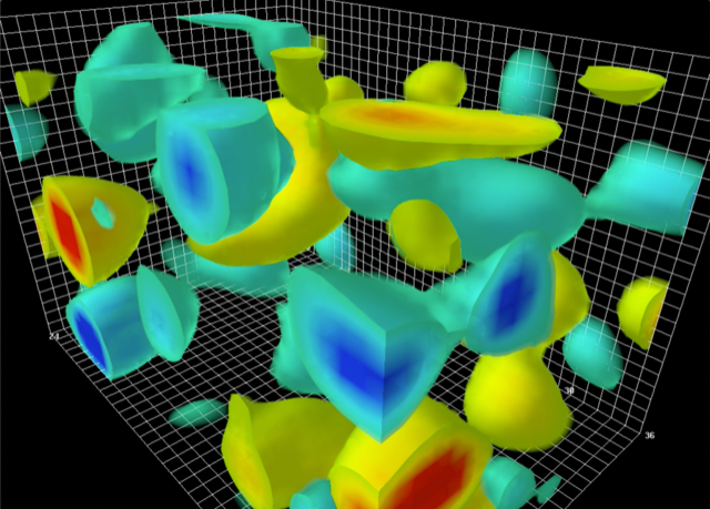
Figure 1: Instantons (yellow) and anti-instantons (blue) configurations in the cooled YM vacuum Moran and Leinweber (2008).

II Instanton effects

The cooled QCD vacuum is populated with strong and inhomogeneous topological gauge configurations, i.e. instantons and anti-instantons as illustrated in Fig. 1 The bulk characteristics of this vacuum were predicted long ago Shuryak (1982)

$$n_{I+\bar{I}}\approx 1\,{\rm fm}^{-4},\,\,\,\,\,\rho\sim\frac{1}{3}\,{\rm fm}\sim\frac{1}{0.6}\,{\rm GeV}^{-1}$$ (1)

for the instanton plus anti-instanton density and size, respectively. They combine in the dimensionless parameter

$$\kappa\equiv\pi^{2}\rho^{4}n_{I+\bar{I}}\approx 3.186\times 10^{-3}$$

a measure of the diluteness of the instanton-anti-instanton ensemble in the QCD vacuum. Previous lattice simulations using cooling methods support these observations - see Schäfer and Shuryak (1998) for a review.

Instanton fields are strong, since their field strengths are large. For the dominant size instantons with $\rho\approx 0.30\,{\rm fm}$ typical for chiral symmetry breaking, the fields are very strong at the center

$$\sqrt{G^{2}_{\mu\nu}(0)}=\sqrt{192}/\rho^{2}\approx 5\,{\rm GeV}^{2}$$

Their scale is comparable to the matching scale in the hard and perturbative matching kernels Ji et al. (2020) which may suggest non-perturbative improvements Liu and Zahed (2021). Their contribution can be assessed using semi-classics. The size distribution of the instantons and anti-instantons in the QCD vacuum is well captured semi-empirically by Hasenfratz (2000); Shuryak (1999)

$$dn(\rho)\sim{d\rho\over\rho^{5}}\big{(}\rho\Lambda_{QCD}\big{)}^{b_{QCD}}\,e^{-\alpha^{\prime}\rho^{2}}$$ (2)

with $b_{QCD}=11N_{c}/3-2N_{f}/3\approx 9$ (one loop) and $\alpha^{\prime}=1/2m_{\rho}^{2}$ (rho meson slope).

III Twist and chiral structures of the DA of the pion

In the QCD instanton vacuum, the pion DA is captured by the vertex $\pi^{-}(p)\rightarrow d_{if\alpha}(k)u^{\dagger}_{jg\beta}(k-p)$, which corresponds formally to the connected amplitude

$$\int_{-\infty}^{+\infty}\frac{p^{+}dz^{-}}{2\pi}e^{-ixp\cdot z}\left<0\left|\overline{u}_{\beta}(0)[0,z]d_{\alpha}(z)\right|\pi^{-}(p)\right>$$

$$=\left(+\frac{if_{\pi}}{4}\gamma^{5}\bigg{(}\not{p}\,\phi^{A}_{\pi^{-}}(x)-\chi_{\pi}\phi_{\pi^{-}}^{P}(x)+i\chi_{\pi}\sigma_{\mu\nu}\frac{p^{\mu}p^{\prime\nu}}{p\cdot p^{\prime}}{\phi_{\pi^{-}}^{\prime\,T}(x)\over{6}}\bigg{)}\right)_{\alpha\beta}$$ (3)

and its conjugate

$$\int_{-\infty}^{+\infty}\frac{p^{\prime-}dz^{+}}{2\pi}e^{ixp^{\prime}\cdot z}\left<\pi^{-}(p^{\prime})\left|\overline{d}_{\beta}(z)[z,0]u_{\alpha}(0)\right|0\right>$$

$$=\left(-\frac{if_{\pi}}{4}\gamma^{5}\bigg{(}\not{p}^{\prime}\,\phi^{A}_{\pi^{-}}(x)+\chi_{\pi}\phi_{\pi^{-}}^{P}(x)-i\chi_{\pi}\sigma_{\mu\nu}\frac{p^{\mu}p^{\prime\nu}}{p\cdot p^{\prime}}{\phi_{\pi^{-}}^{\prime\,T}(x)\over{6}}\bigg{)}\right)_{\alpha\beta}$$ (4)

up to twist-3. $[x,y]$ refers to the gauge link, $\sigma_{\mu\nu}=\frac{i}{2}[\gamma_{\mu},\gamma_{\nu}]$, $\{\alpha,\beta\}$ represent spinor indices, and $\phi^{T\prime}_{\pi}(x)=\partial_{x}\phi^{T}_{\pi}(x)$. (III-III) are explicitly odd under P parity. Note that the 4-vector $p^{\prime}_{\mu}$ appears in the DA of a pion with 4-vector $p_{\mu}$, in reference to the conjugate light-cone direction, with generally no relation to the second pion. In the DA of a pion with momentum $p^{\prime}_{\mu}$, the exchange $p\leftrightarrow p^{\prime}$ needs to be enforced, effectively flipping the sign of the last term.

In (III), (III), and subsequent derivations, the ket $|\pi^{-}(P)\rangle$ refers to the physical negative-pion state. (Note the switch in flavors if the current $J_{\pi^{-}}(x)=\bar{d}(x)i\gamma^{5}u(x)$ is used to define the pion state). (III-III) can be inverted, to recast the pion twist-2 and twist-3 light-cone wavefunctions in explicit form

$$\phi_{\pi^{-}}^{A}(x)=\frac{1}{if_{\pi}}\int_{-\infty}^{+\infty}\frac{dz^{-}}{2\pi}e^{ixp\cdot z}\left<0\left|\overline{u}(0)\gamma^{+}\gamma_{5}[0,z]d(z)\right|\pi^{-}(p)\right>$$ (5a)

$$\phi^{P}_{\pi^{-}}(x)=\frac{p^{+}}{f_{\pi}\chi_{\pi}}\int_{-\infty}^{+\infty}\frac{dz^{-}}{2\pi}e^{ixp\cdot z}\left<0\left|\overline{u}(0)i\gamma_{5}[0,z]d(z)\right|\pi^{-}(p)\right>$$ (5b)

$${\phi^{T\prime}_{\pi^{-}}(x)}=\frac{6}{f_{\pi}\chi_{\pi}}\frac{p^{\mu}p^{\prime\nu}p^{+}}{p\cdot p^{\prime}}\int_{-\infty}^{+\infty}\frac{dz^{-}}{2\pi}e^{ixp\cdot z}\left<0\left|\overline{u}(0)\sigma_{\mu\nu}\gamma_{5}[0,z]d(z)\right|\pi^{-}(p)\right>$$ (5c)

with all DAs normalized to 1. The prime in the last relation refers to $\partial_{x}\phi_{\pi^{-}}^{T}(x)$. The leading twist-2 DA $\phi^{A}_{\pi}(x)$ is chirally-diagonal. Its normalization to 1 is fixed by the weak pion decay constant $f_{\pi}\approx 130\,{\rm MeV}$,

$$\left<0\left|\overline{u}(0)\gamma^{\mu}{(1-\gamma^{5})}d(0)\right|\pi^{-}(p)\right>=-{\rm Tr}\bigg{(}\gamma^{\mu}{(1-\gamma^{5})}\bigg{(}\frac{if_{\pi}}{4}\gamma^{5}\not{p}\bigg{)}\bigg{)}\,\int_{0}^{1}dx\,\phi^{A}_{\pi^{-}}(x)\equiv if_{\pi}\,p^{\mu}$$ (6)

Isospin symmetry and charge conjugation force $\phi_{\pi}(x)=\phi_{\pi}(\overline{x})$. The two twist-3 independent DAs $\phi^{P}_{\pi}(x)$ and $\phi_{\pi}^{T}(x)$ are chirally non-diagonal Geshkenbein and Terentev (1982). They are tied by the current identity

$$\partial^{\nu}\big{(}\overline{u}(0)\sigma_{\mu\nu}\gamma_{5}d(z)\big{)}=-\partial_{\mu}\big{(}\overline{u}(0)i\gamma_{5}d(z)\big{)}+m\,\overline{u}(0)\gamma_{\mu}\gamma_{5}d(z)$$ (7)

and share the same couplings. The value of the dimensionful coupling constant $\chi_{\pi}$ can be fixed by the divergence of the axial-vector current and the PCAC relation

$$(m_{u}+m_{d})\left<0\left|\overline{u}(0)i\gamma^{5}d(0)\right|\pi^{-}(p)\right>=$$

$$-(m_{u}+m_{d})\,{\rm Tr}\bigg{(}i\gamma^{5}\bigg{(}\frac{if_{\pi}}{4}\gamma^{5}\chi_{\pi}\bigg{)}\bigg{)}\,\int_{0}^{1}dx\,\phi_{\pi}^{P}(x)=(m_{u}+m_{d})\,f_{\pi}\chi_{\pi}$$ (8)

with $\phi_{\pi}^{P}(x)$ normalized to 1. Using the Gell-Mann-Oakes-Renner relation

$$f_{\pi}^{2}m_{\pi}^{2}=-2(m_{u}+m_{d})\left<\overline{q}q\right>$$ (9)

with $|\left<\overline{q}q\right>|\approx(240\,{\rm MeV})^{3}$, yield

$$\chi_{\pi}=\frac{m_{\pi}^{2}}{(m_{u}+m_{d})}$$ (10)

The values of the quark masses depend on the renormalization scale $\mu$. Lattice simulations with fine lattices use $\mu\approx 2$ GeV. However, for the DAs it is more appropiate to use a softer $\mu\approx 1/\rho$ renormalization with slightly larger current quark masses giving $\chi_{\pi}\approx 1.2$ GeV.

The twist-3 pion DAs asymptote $\phi_{\pi^{-}}^{P}(x)\rightarrow 1$ and $\phi_{\pi^{-}}^{T}(x)\rightarrow 6x\bar{x}$ owing to their conformal collinear spin, with $\phi_{\pi^{-}}^{T\prime}(x)\rightarrow 6(\bar{x}-x)$. At large $Q^{2}$ their contribution is subleading in the pion electromagnetic form factor Shuryak and Zahed (2020)

$$\frac{f_{\pi}^{2}\chi_{\pi}^{2}}{Q^{4}}\int dx_{1}dx_{2}\,{1\over\bar{x}_{1}\bar{x}_{2}}\bigg{[}\bigg{(}\frac{1}{\bar{x}_{2}}-1\bigg{)}+(\bar{x}_{2}-x_{2})\bigg{(}\frac{1}{\bar{x}_{2}}+1\bigg{)}=2\bar{x}_{2}\bigg{]}=2\frac{f_{\pi}^{2}\chi_{\pi}^{2}}{Q^{4}}\int\frac{dx_{1}}{\bar{x}_{1}}\,\,$$ (11)

IV Twist-3 QDA of the pion and kaon

The quasi-pion distribution distribution amplitudes (qPDA) variants of (5) are

$$\tilde{\phi}^{A}_{\pi^{-}}(x,P_{z})=\frac{i}{f_{\pi}}\int_{-\infty}^{\infty}\frac{dz}{2\pi}e^{i\frac{x-\bar{x}}{2}P_{z}z}\langle 0|\bar{u}(z_{-})\gamma^{z}\gamma^{5}[z_{-},z_{+}]d(z_{+})|\pi^{-}(p)\rangle$$ (12a)

$$\tilde{\phi}_{\pi^{-}}^{P}(x,P_{z})=\frac{iP_{z}}{f_{\pi}\chi_{\pi}}\int_{-\infty}^{\infty}\frac{dz}{2\pi}e^{i\frac{x-\bar{x}}{2}P_{z}z}\langle 0|\bar{u}(z_{-})\gamma^{5}[z_{-},z_{+}]d(z_{+})|\pi^{-}(p)\rangle$$ (12b)

$$\tilde{\phi}_{\pi^{-}}^{T\prime}(x,P_{z})=\frac{6P_{z}}{f_{\pi}\chi_{\pi}}\frac{P^{\mu}n^{\prime\nu}}{P\cdot n^{\prime}}\int_{-\infty}^{\infty}\frac{dz}{2\pi}e^{i\frac{x-\bar{x}}{2}P_{z}z}\langle 0|\bar{u}(z_{-})\sigma_{\mu\nu}\gamma^{5}[z_{-},z_{+}]d(z_{+})|\pi^{-}(p)\rangle$$ (12c)

where $z$ is a space-like separation, $z_{\pm}=\pm z/2$, and $n^{\mu}=\{0,0,0,1\}$ is the unit-vector along the linear quark-separation (space-like, $z$-direction here). For the corresponding $K^{-}$ qPDAs, one would simply replace the $d$-quark with the $s$-quark, and switch to the state $|K^{-}(P)\rangle$. For finite $P_{z}$, the qPDAs can be matched with the corresponding light-cone DA counterparts (5) by an integration kernel, calculable order-by-order in powers of $\frac{\mu}{P_{z}}$ where $\mu$ represents any other mass-scale present Ji (2013) Ji et al. (2020). However we will be taking the limit $P_{z}\rightarrow\infty$, where the matching becomes trivial $\tilde{\phi}(x,P_{z}\rightarrow\infty)\rightarrow\phi(x)$. Modulo $x$-independent prefactors, the twist-3 distributions only differ from the twist-2 distribution in their Dirac structure. We write this common factor as:

$$\int_{-\infty}^{\infty}\frac{dz}{2\pi}e^{i\frac{x-\bar{x}}{2}P_{z}z}\langle 0|\bar{u}(z_{-})\Gamma[z_{-},z_{+}]d(z_{+})|\pi^{-}(p)\rangle$$ (13)

Following the prescription of the present authors’ previous paper  Kock et al. (2020), we insert the physical pion source and resum planar diagrams to leading order in the diluteness factor $\alpha\sim\sqrt{\kappa}$ to get

$$\frac{-P^{2}}{P_{z}g_{\pi}}\int\frac{d^{4}k}{(2\pi)^{4}}\delta\left(x-\frac{1}{2}-\frac{k_{z}}{P_{z}}\right)\textrm{Tr}\left[\Gamma S_{1}O_{5}(P,p_{1})S_{2}\right]$$ (14)

where in going from (13) to (14), $S_{1}$ refers to the $u$-quark and $S_{2}$ refers to the $d$-quark (or $s$-quark for the negative Kaon). We have subsumed notation for the pion’s on-shell condition $\lim P^{2}\rightarrow m_{\pi}^{2}$. The trace is over all indices, and $p_{1,2}^{\mu}=k^{\mu}\pm P^{\mu}/2$ is the momentum carried by each quark flavor. The re-summed quark propagator $S_{1,2}\equiv S(p_{1,2},m_{1,2})$ is

$$S(k,m) =\bigg{(}\frac{1}{\not{k}-i\sigma(k,m)}\bigg{)}\approx\frac{1}{k^{2}+M^{2}(0,m)}\left(\not{k}+iM(k,m)\right)$$ (15)

where $m$ is the current mass of the individual quark. The effective mass at LO in $\alpha$ is given by $\sigma(k,m)\approx M(k,m)+\mathcal{O}(\alpha^{2})$

$$\begin{split}M(k,m)&=\frac{M(k)}{\left(1+\xi^{2}\right)^{1/2}+\xi}+m\\ M(k)&=M(0)\left(\left|z\left(I_{0}K_{0}-I_{1}K_{1}\right)^{\prime}\right|^{2}\right)_{z=\frac{k\rho}{2}}\\ \xi&=\frac{mM(0)\rho^{2}}{8\pi^{2}\kappa}\end{split}$$ (16)

with $M(k)\equiv M(k,0)$ throughout. In the above approximation we have dropped the term $\Delta\sigma^{2}\equiv\sigma^{2}(k)-\sigma^{2}(0)$ because it only provides a correction to our final integrals which is subleading in $\alpha$. The benefit of this approximation is that our integrals will have vastly simplified $k^{\mu}$ dependence. In Fig. 2 we show the induced constituent quark mass (16) for the parameters of the instanton vacuum. In Fig. 2a we show $M(p,0)$ solid-red curve versus $p$ in GeV units. The spread corresponds to $M(0)=383\pm 39$ MeV and $\rho=0.313\pm 0.016$ fm. The open-circles are lattice generated quark masses in Coulomb gauge Bowman et al. (2004). In Fig. 2b we show the dependence of the ratio $M(0,m)/M(0,0)$ on the current mass by the solid-blue curve for fixed $\xi$, and by the dashed-red curve for $\xi\ll 1$.

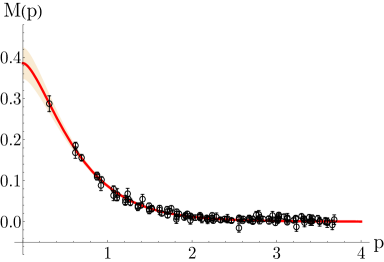
(a)

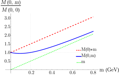
(b)

Figure 2: a: Effective quark mass M(p)=M(p,0), both axes GeV; b: Effective quark mass ratio, as a function of current quark mass. See text.

The re-summed pseudoscalar pion vertex is

$$O_{5}(P,p_{1})\approx\gamma^{5}\left(1+F_{5}(P,p_{1})\right)+\alpha\bar{F}_{5}(P,p_{1})+\mathcal{O}(\alpha^{2})$$ (17)

$$F_{5}(P,p_{1})\,\overset{P^{2}\rightarrow m_{\pi}^{2}}{\approx}\,\frac{g_{\pi}}{f_{\pi}}\sqrt{M(p_{1})}\frac{1}{P^{2}+m_{\pi}^{2}}\sqrt{M(p_{2})}$$ (18)

where $g_{\pi}$ is the pseudoscalar pion-quark-quark coupling. For an explicit calculation of $g_{\pi}$ in the RIV framework, see section III.C in Kock et al. (2020). Expanding to first order in $\alpha$, [14] keeping in mind that $M(k)=\alpha\sigma_{0}(k)$, the common factor becomes

$$\begin{split}\frac{-P^{2}}{P_{z}g_{\pi}}\int\frac{d^{4}k}{(2\pi)^{4}}&\,\delta\left(x-\frac{1}{2}-\frac{k_{z}}{P_{z}}\right)\\ \times\Bigg{\{}\,&\textrm{Tr}\left[\Gamma\frac{\not{p}_{1}}{p_{1}^{2}+M_{1}^{2}}\gamma^{5}\left(1+F_{5}(p_{1},p_{2})\right)\frac{\not{p}_{2}}{p_{2}^{2}+M_{2}^{2}}\right]\\ &+\textrm{Tr}\left[\Gamma\left(\frac{i\alpha\sigma_{0}(p_{1})}{p_{1}^{2}+M_{1}^{2}}\right)\gamma^{5}\left(1+F_{5}(p_{1},p_{2})\right)\frac{\not{p}_{2}}{p_{2}^{2}+M_{2}^{2}}\right]\\ &+\textrm{Tr}\left[\Gamma\frac{\not{p}_{1}}{p_{1}^{2}+M_{1}^{2}}\gamma^{5}\left(1+F_{5}(p_{1},p_{2})\right)\left(\frac{i\alpha\sigma_{0}(p_{2})}{p_{2}^{2}+M_{2}^{2}}\right)\right]\\ &+\textrm{Tr}\left[\Gamma\frac{\not{p}_{1}}{p_{1}^{2}+M_{1}^{2}}\alpha\bar{F}_{5}(P,p_{1})\frac{\not{p}_{2}}{p_{2}^{2}+M_{2}^{2}}\right]\Bigg{\}}+\mathcal{O}(\alpha^{2})\end{split}$$ (19)

with $M_{1,2}\equiv M(0,m_{1,2})$ being the effective mass for each quark.

In (19) there are four traces: the first is of order $\alpha^{0}$, the next three are of order $\alpha^{1}$. If $\Gamma$ contains an odd number of $\gamma$’s (e.g. $\Gamma=\gamma^{z}\gamma^{5}$), the first trace term at order $\alpha^{0}$ has vanishing Dirac trace, whereas the remaining three do not have vanishing Dirac trace. This is the case when calculating the twist-2 qPDA. However if $\Gamma$ contains an even number of $\gamma$’s (e.g. $\Gamma=\gamma^{5},\,\sigma_{\mu\nu}\gamma^{5}$), then the first term has nonvanishing Dirac trace. At next to leading order (NLO) in $\alpha$, the second and third terms vanish. The fourth term involving $\bar{F}_{5}$ does not have vanishing Dirac trace, and requires special attention. This is the case with the twist-3 distributions, which we are considering here. In our previous paper Kock et al. (2020) we showed that this term vanishes for the axial-vector twist-2 DA, $\Gamma=\gamma^{z}\gamma^{5}$. We now make explicit the leading contributions in $\alpha\sim\sqrt{\kappa}$ to the twist-3 DAs, $\phi^{P}_{0}(x)$ and $\phi^{T}_{0}(x)$. We also recap the similar expression for the twist-2 DA, $\phi^{A}_{0}(x)$.

IV.1 Pseudoscalar, $\Gamma=\gamma^{5}$

The calculation of $\tilde{\phi}^{P}_{0}(x,)$ begins by reinstating the appropriate prefactor in (19). Out of the first three zero-mode contributions in (19), only the first has non-vanishing Dirac trace

$$\tilde{\phi}^{P}_{0}(x,P_{z}) =\frac{iP_{z}}{f_{\pi}\chi_{\pi}}\frac{-P^{2}}{P_{z}g_{\pi}}\int\frac{d^{4}k}{(2\pi)^{4}}\,\delta\left(x-\frac{1}{2}-\frac{k_{z}}{P_{z}}\right)\textrm{Tr}\left[\gamma^{5}\frac{\not{p}_{1}}{p_{1}^{2}+M_{1}^{2}}\gamma^{5}\left(1+F_{5}(p_{1},p_{2})\right)\frac{\not{p}_{2}}{p_{2}^{2}+M_{2}^{2}}\right]$$

$$=\frac{4iN_{c}}{f_{\pi}^{2}\chi_{\pi}}\int\frac{d^{2}k_{\perp}dk_{4}dk_{z}}{(2\pi)^{4}}\delta\left(x-\frac{1}{2}-\frac{k_{z}}{P_{z}}\right)\left(M(p_{1})M(p_{2})\right)^{1/2}\frac{p_{1}\cdot p_{2}}{(p_{1}^{2}+M_{1}^{2})(p_{2}^{2}+M_{2}^{2})}$$

$$=\frac{4iN_{c}P_{z}}{f_{\pi}^{2}\chi_{\pi}}\int\frac{d^{2}k_{\perp}dk_{4}}{(2\pi)^{4}}\left(M(p_{1})M(p_{2})\right)^{1/2}\frac{p_{1}\cdot p_{2}}{(p_{1}^{2}+M_{1}^{2})(p_{2}^{2}+M_{2}^{2})}$$ (20)

where the delta-function has set $P_{1,z}=xP_{z}$ and $P_{2,z}=\bar{x}P_{z}$. Since

$$p_{1}-p_{2}=P\implies p_{1}\cdot p_{2}=\frac{1}{2}\left[p_{1}^{2}+p_{2}^{2}-m_{\pi}^{2}\right]$$ (21)

the last term in (IV.1) can be recast in the form

$$\tilde{\phi}^{P}_{0}(x,P_{z})=\frac{2iN_{c}P_{z}}{f_{\pi}^{2}\chi_{\pi}}\int\frac{d^{2}k_{\perp}dk_{4}}{(2\pi)^{4}}\left(M(p_{1})M(p_{2})\right)^{1/2}\frac{p_{1}^{2}+p_{2}^{2}-m_{\pi}^{2}}{(p_{1}^{2}+M_{1}^{2})(p_{2}^{2}+M_{2}^{2})}$$ (22)

Notice that for the $k_{4}$-integration, the pole and branch point structure is exactly the same as in the twist-2 case. Therefore we evaluate in the same way, by Wick-rotating and shifting in $k_{4}$, into the Minkowski domain as we detail in appendix A. Taking the final limit $P_{z}\rightarrow\infty$, including the finite pion mass Kock et al. (2020), and simplifying the pre-factor using $\chi_{\pi}=-2\langle\bar{\psi}\psi\rangle/f_{\pi}^{2}$, the final result for the leading-order pseudoscalar DA is

$$\tilde{\phi}^{P}_{0}(x)=i\frac{N_{c}}{2\langle\bar{\psi}\psi\rangle}\frac{\theta(x\bar{x})}{x\bar{x}}\int\frac{d^{2}k_{\perp}}{(2\pi)^{3}}\,M\left(\frac{k_{\perp}}{\lambda\sqrt{x\bar{x}}}\right)\frac{k_{\perp}^{2}+\bar{x}^{2}M_{1}^{2}+x^{2}M_{2}^{2}}{k_{\perp}^{2}+\bar{x}M_{1}^{2}+xM_{2}^{2}-x\bar{x}m_{\pi}^{2}}$$ (23)

The requisite $x\leftrightarrow\bar{x}$, $m_{1}\leftrightarrow m_{2}$ symmetry is manifest. For plotting we use phenomenological values $M(0)=383\,\textrm{MeV}$, $|\langle\bar{\psi}\psi\rangle|=(240\,\textrm{MeV})^{3}$, and $\rho=0.313\,\textrm{fm}$. The normalizing values of $\lambda$ are provided in table 1 in appendix B. Unevolved plots of (23) are shown in Fig. 3 for both the limit of a small instanton size $\rho\rightarrow 0$ and typical instanton size $\rho=0.313\,\textrm{fm}$. For the pion, there is no perceptible difference in (23) between using physical masses ($m_{\pi}=140\,\textrm{MeV}$, $m_{u}=3\,\textrm{MeV}$, $m_{d}=7\,\textrm{MeV}$) and the chiral counterparts ($m_{\pi,u,d}=0$). For the kaon we use $m_{K}=494\,\textrm{MeV}$, $m_{u}=3\,\textrm{MeV}$, $m_{s}=136\,\textrm{MeV}$. The small-size instanton limit ($\rho\rightarrow 0$) corresponds to very high resolution and is commensurate with the QCD asymptotic result as expected.

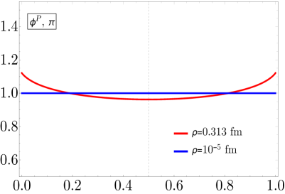
(a)

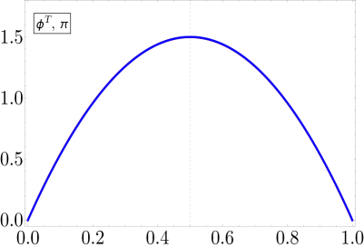
(b)

Figure 3: Pseudoscalar and pseudotensor pion DAs at different instanton sizes or resolution. The $\rho\approx 0$ curves (solid blue) are indiscernible from the asymptotic forms. For the pseudotensor DA $\phi^{T}$, both for phenomenological and small $\rho$, the curves are indistinguishable from the asymptotic form $6x\bar{x}$.

IV.2 Pseudotensor, $\Gamma=\sigma_{\mu\nu}\gamma^{5}$

The only difference with the pseudoscalar case will be that instead of having a factor $i\textrm{Tr}\left[\not{p_{1}}\not{p_{2}}\right]$, we will have

$$6\frac{P_{\mu}n_{\nu}}{P\cdot n}\textrm{Tr}\left[\sigma^{\mu\nu}\not{p_{1}}\not{p_{2}}\right] =-24i\frac{P_{\mu}n_{\nu}}{P\cdot n}\left(p_{1}^{\mu}p_{2}^{\nu}-p_{2}^{\mu}p_{1}^{\nu}\right)$$

$$=\frac{-24i}{P\cdot n}\left[(P\cdot p_{1})(n\cdot p_{2})-(n\cdot p_{1})(P\cdot p_{2})\right]$$ (24)

where $n^{\mu}$ is the tangent vector to the spacelike quark separation line in (12), $n^{\mu}=\hat{z}^{\mu}$. Making this replacement in (IV.1), we get

$$\tilde{\phi}^{T\prime}_{0}(x,P_{z})=\frac{-24iN_{c}}{f_{\pi}^{2}\chi_{\pi}}\int\frac{d^{2}k_{\perp}dk_{4}}{(2\pi)^{4}}\left(M(p_{1})M(p_{2})\right)^{1/2}\frac{(P\cdot p_{1})(n\cdot p_{2})-(n\cdot p_{1})(P\cdot p_{2})}{\left(p_{1}^{2}+M_{1}^{2}\right)\left(p_{2}^{2}+M_{2}^{2}\right)}$$ (25)

As before, we Wick-rotate and shift the $k_{4}$ integration, $k_{4}\rightarrow i(k_{4}+(x-\frac{1}{2}E))$, leaving us with

$$\tilde{\phi}^{T\prime}_{0}(x,P_{z})=\frac{24N_{c}}{f_{\pi}^{2}\chi_{\pi}}\int\frac{d^{2}k_{\perp}dk_{4}}{(2\pi)^{4}}\left(M(y_{1})M(y_{2})\right)^{1/2}\frac{(P\cdot y_{1})(n\cdot y_{2})-(n\cdot y_{1})(P\cdot y_{2})}{\left(y_{1}^{2}+M_{1}^{2}\right)\left(y_{2}^{2}+M_{2}^{2}\right)}$$ (26)

To evaluate the integrand we use the same kinematics as in (34). To perform the $k_{4}$ integral, we follow the same procedure as in the pseudoscalar case - use the modified effective mass, then integrate the remaining rational function using Cauchy’s residue theorem. The final result for the integrated $\phi^{T}(x)$ is

$$\tilde{\phi}^{T}_{0}(x) =\frac{-3iN_{c}}{\langle\bar{\psi}\psi\rangle}\theta(x\bar{x})\int_{0}^{x}dv\,\int\frac{d^{2}k_{\perp}}{(2\pi)^{3}}M\left(\frac{k_{\perp}}{\lambda\sqrt{v\bar{v}}}\right)\frac{1}{v\bar{v}}\frac{(\bar{v}-v)k_{\perp}^{2}+\bar{v}^{2}M_{1}^{2}-v^{2}M_{2}^{2}}{k_{\perp}^{2}-v\bar{v}m_{\pi}^{2}+\bar{v}M_{1}^{2}+vM_{2}^{2}}$$

Again, the requisite $x\leftrightarrow\bar{x}$, $m_{1}\leftrightarrow m_{2}$ symmetry is manifest (the integrand is odd under this transformation). Unevolved plots of (IV.2) are shown in Fig. 3 for phenomenological and limiting values of $\rho$. In the case that $\rho\rightarrow 0$ (high resolution), the pseudotensor DA approaches its asymptotic form. Once again, the normalizing values of $\lambda$ are given in table 1 in appendix B.

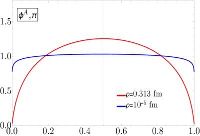
(a)

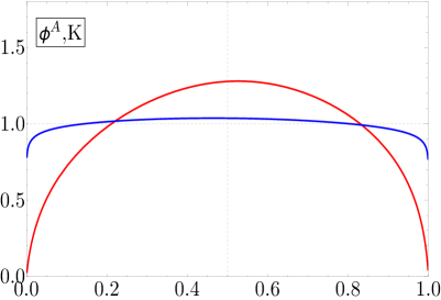
(b)

Figure 4: Twist-2 (axial-vector) pion and kaon DAs at different instanton sizes or resolution. The normalizing values of $\lambda$ for the $\rho=10^{-5}\,\textrm{fm}$ curves are as follows: $\lambda_{\pi}=7.51$, $\lambda_{K}=9.7$ (for the phenomenological curves see Appendix VII.2). For both the pion and kaon, the $\rho\approx 0$ curves (solid blue) tend toward a normalized step-function $\theta(x\bar{x})$.

IV.3 Axial-vector, Twist-2, $\Gamma=\gamma^{z}\gamma^{5}$

Here we generalize a key expression from our previous paper Kock et al. (2020): the twist-2 DA at leading order in $\alpha$, now including finite current quark masses $m_{1,2}$ for the pseudoscalar meson $P$. It is given by

$$\phi^{A}_{P}(x)\approx\frac{2N_{c}}{f_{P}^{2}}\theta(x\bar{x})\int\frac{d^{2}k_{\perp}}{(2\pi)^{3}}M\left(\tilde{k}_{\perp}\right)\,\frac{\bar{x}M\left(\tilde{k}_{\perp},m_{1}\right)+xM\left(\tilde{k}_{\perp},m_{2}\right)}{k_{\perp}^{2}-x\bar{x}m_{P}^{2}+\bar{x}M_{1}^{2}+xM_{2}^{2}}$$ (28)

with $\tilde{k}_{\perp}={k_{\perp}}/{\lambda\sqrt{x\bar{x}}}$. We use $f_{\pi}=130\,\textrm{MeV}$ for massive pions and $f_{K}=155\,\textrm{MeV}$ for massive kaons. Unevolved plots of (28) are shown in Fig. 4 for phenomenological and limiting values of $\rho$. For $\rho\rightarrow 0$ the curves tend towards a normalized step-function, rather than towards the asymptotic distribution $6x\bar{x}$. This type of curve has been noted for chiral quark models with point interactions Broniowski and Ruiz Arriola (2017) Jia and Vary (2019), and some bound-state resummations Ding et al. (2020).

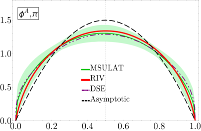
(a)

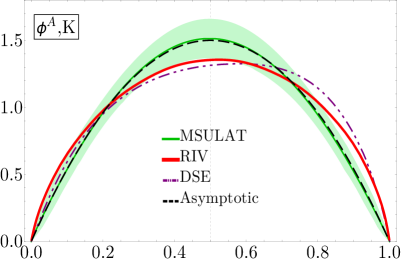
(b)

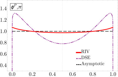
(c)

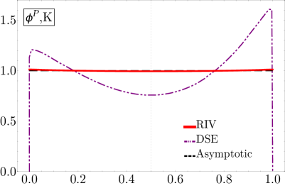
(d)

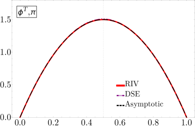
(e)

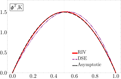
(f)

Figure 5: ERBL evolution of DAs, compared with data. All curves are given at $Q=2\,\textrm{GeV}$, except for LFCQM de Melo et al. (2016) (blue-dotted) which is renormalized in a different scheme. RIV (red-solid-thick) represents our current work, the random instanton vacuum approach, given by equations (23), (IV.2), and (28). MSULAT curves (green-solid-bands) are recent lattice computations utilizing the LaMET framework Zhang et al. (2020). DSE curves (purple-dash-dot-dot) are from Shi et al. (2015) which utilized Dyson-Schwinger equations with Bethe-Salpeter amplitudes.

V QCD Evolution

The two-particle twist 2 & 3 DAs in the random instanton vacuum (RIV) are defined at a low renormalization scale set by the typical inverse instanton size $Q_{0}=1/\rho=631$ GeV. Assuming factorization, their forms at higher renormalization scales follow from QCD evolution equations

$$\phi^{A}(x,Q) =6x\bar{x}\sum_{n=0}^{\infty}a_{n}(Q_{0})\left(\frac{\alpha_{s}(Q^{2})}{\alpha_{s}(Q^{2}_{0})}\right)^{\gamma_{n}^{A}/\beta_{0}}C_{n}^{3/2}(x-\bar{x})$$ (29a)

$$\phi^{P}(x,Q) =1+\sum_{n=1}^{\infty}b_{n}(Q_{0})\left(\frac{\alpha_{s}(Q^{2})}{\alpha_{s}(Q^{2}_{0})}\right)^{\gamma_{n}^{P}/\beta_{0}}C_{n}^{1/2}(x-\bar{x})$$ (29b)

$$\phi^{T}(x,Q) =6x\bar{x}\left[1+\sum_{n=1}^{\infty}c_{n}(Q_{0})\left(\frac{\alpha_{s}(Q^{2})}{\alpha_{s}(Q^{2}_{0})}\right)^{\gamma_{n}^{T}/\beta_{0}}C_{n}^{3/2}(x-\bar{x})\right]$$ (29c)

with the anomalous dimensions $\gamma_{n}^{A,P,T}$ given by Shifman and Vysotsky (1981)

$$\gamma_{n}^{A} =C_{F}\left[-3+4\sum_{j=1}^{n+1}\frac{1}{j}-\frac{2}{(n+1)(n+2)}\right]$$ (30a)

$$\gamma_{n}^{P} =C_{F}\left[-3+4\sum_{j=1}^{n+1}\frac{1}{j}-\frac{8}{(n+1)(n+2)}\right]$$ (30b)

$$\gamma_{n}^{T} =C_{F}\left[-3+4\sum_{j=1}^{n+1}\frac{1}{j}\right]$$ (30c)

Here $C_{n}^{m}(z)$ are Gegenbauer polynomials, $C_{F}=(N_{c}^{2}-1)/2N_{c}$ is the quadratic-Casimir in the fundamental representation, $\alpha_{s}(Q^{2})=4\pi/\left(\beta_{0}\ln(Q^{2}/\Lambda^{2})\right)$ is the one-loop running QCD coupling, $\beta_{0}=\frac{11}{3}N_{c}-\frac{2}{3}N_{f}$, and $\Lambda=250\,\textrm{MeV}$. One can easily verify that the normalizations are preserved under QCD evolution, as they should be. Owing to the orthogonality of the Gegenbauer polynomials, the initial coefficients are given by

$$a_{n}(Q_{0}) =\frac{2(2n+3)}{3(n+1)(n+2)}\int_{0}^{1}dy\,C_{n}^{3/2}(y-\bar{y})\phi^{A}(y,Q_{0})$$ (31a)

$$b_{n}(Q_{0}) =(2n+1)\int_{0}^{1}dy\,C_{n}^{1/2}(y-\bar{y})\phi^{P}(y,Q_{0})$$ (31b)

$$c_{n}(Q_{0}) =\frac{2(2n+3)}{3(n+1)(n+2)}\int_{0}^{1}dy\,C_{n}^{3/2}(y-\bar{y})\phi^{T}(y,Q_{0})$$ (31c)

The twist-2 & twist-3 DAs, evolved to $Q=2\,\textrm{GeV}$, are shown in fig.5. All curves are shown at the same renormalization scale. Our twist-2 pion DA shows a shape slightly broader than the asymptotic form. This shape has been seen in recent lattice calculations Zhang et al. (2017)Zhang et al. (2020). In some light-front constituent quark models, a shape slightly narrower than the asymptotic form is seen - we do not display this curve in fig.5a because of a mismatch in renormalization schemes de Melo et al. (2016). The empirical pion twist-2 DA extracted from dijet data by the E791 collaboration is in agreement with all curves shown fig.5a, though the precise shape is obscured by uncertainties Aitala (2001). The same broad shape is seen in our twist-2 kaon DA, fig.5b, although we see a smaller asymmetry than other phenomenological approaches.

The general behavior of all our DAs show agreement with those denoted DSE Shi et al. (2015), except that our curves are closer to the respective asymptotic forms. This is most notable in the pseudoscalar DAs, where our curves are remarkably closer to the asymptotic form. Although our kaon’s pseudoscalar DA seems to lack asymmetry, especially compared to the pion’s pseudoscalar DA, this is only because the overall scale of all its Gegenbauer moments are smaller, thereby making its difference from the asymptotic form indiscernible. We can see this with a comparison of the first two non-trivial Gegenbauer moments - the ratio $b_{1}/b_{2}$ is nearly an order of magnitude larger for the kaon compared to the pion.

$$b_{1}^{\pi}(Q_{0}) =-8.4\times 10^{-5} b_{2}^{\pi}(Q_{0}) =1.74\times 10^{-2} \left|\frac{b_{1}^{\pi}(Q_{0})}{b_{2}^{\pi}(Q_{0})}\right| =4.82\times 10^{-3}$$ (32a)

$$b_{1}^{K}(Q_{0}) =-1.41\times 10^{-4} b_{2}^{K}(Q_{0}) =3.46\times 10^{-3} \left|\frac{b_{1}^{K}(Q_{0})}{b_{2}^{K}(Q_{0})}\right| =4.07\times 10^{-2}$$ (32b)

VI Conclusions

Cooled lattice gauge configurations display strongly inhomogeneous instanton and anti-instanton configurations. The dilute QCD instanton vacuum in its simplified RIV form capture the essentials physics of these tunneling configurations at low resolution. Each tunneling traps a zero mode of a given chirality for each flavor, breaking dynamically chiral symmetry. The disordering of these zero modes leads to a multitude of multiquark condensates and a running constituent quark mass Schäfer and Shuryak (1998); Zahed (2021).

In the RIV the pion quasi-DA is a state made of zero-modes and non-zero-modes that interact collectively. While still complex, this state can be organized in terms of the RIV diluteness factor $\alpha\sim\sqrt{\kappa}$. In leading order in $\alpha$, the twist-2 contribution to the pion quasi-DA involves both the zero-modes and non-zero-modes as we have analyzed in details in Kock et al. (2020) and smoothly yields the pion DA in the large momentum limit. quasi-DA are dominated solely by the zero-modes owing to their pseudo-scalar and pseudotensor content. They also yield smoothly the pion DA in the large momentum limit. In all cases the DA follows from the large momentum limit of the quasi-DA.

Our evolved results for the twist-2 (axialvector) and twist-3 (tensor) pion and kaon DA amplitudes, are very close to the DSE results, and consistent with the recently reported lattice results for the twist-2. Our evolved results for the twist-3 (pseudoscalar) for the pion and kaon DA amplitudes are different from those obtained using the DSE, but very close to the QCD asymptotic results. It is rather remarkable, that our pion and kaon DA amplitudes probe specifically the running emergent topological quark mass in the dilute RIV, which is the dominant component of the QCD vacuum at low resolution.

Acknowledgements

This work is supported by the Office of Science, U.S. Department of Energy under Contract No. DE-FG-88ER40388.

VII Appendices

VII.1 Details of Eq. 23

We start from (22) and perform the analytical continuation $k_{4}\rightarrow ik_{4}$, followed by the shift $k_{4}\rightarrow k_{4}+(x-\frac{1}{2})P_{z}$. The result is

$$\tilde{\phi}^{P}_{0}(x,P_{z})=\frac{2iN_{c}P_{z}}{f_{\pi}^{2}\chi_{\pi}}\int\frac{d^{2}k_{\perp}(idk_{4})}{(2\pi)^{4}}\left(M(y_{1})M(y_{2})\right)^{1/2}\frac{y_{1}^{2}+y_{2}^{2}-m_{\pi}^{2}}{(y_{1}^{2}+M_{1}^{2})(y_{2}^{2}+M_{2}^{2})}$$ (33)

where

$$\begin{split}y_{1}^{\mu}&=\left(\vec{k}_{\perp},xP_{z},i(k_{4}+xE)\right)\\ y_{1}^{2}&=-k_{4}(k_{4}+2xE)+k_{\perp}^{2}-x^{2}m_{\pi}^{2}-i\epsilon\\ y_{1}^{2}+M_{1}^{2}&=-(k_{4}-k_{4+})(k_{4}-k_{4-})\\ &\\ y_{2}^{\mu}&=\left(\vec{k}_{\perp},-\bar{x}P_{z},i(k_{4}-\bar{x}E)\right)\\ y_{2}^{2}&=-k_{4}(k_{4}-2\bar{x}E)+k_{\perp}^{2}-\bar{x}^{2}m_{\pi}^{2}-i\epsilon\\ y_{2}^{2}+M_{2}^{2}&=-(k_{4}-\bar{k}_{4+})(k_{4}-\bar{k}_{4-})\end{split}$$ (34)

The emergent constituent quark mass $M(y)$ is characterized by branch-points. In Kock et al. (2020) we have shown that the analysis retaining the branch points in $M(y)$ is similar to the one following from the modified effective mass at large $P_{z}$,

$$M(y)\rightarrow M\left(\frac{k_{\perp}}{\lambda\sqrt{|x\bar{x}|}}\right)$$ (35)

This removes the explicit $k_{4}$-dependence in $M(y)$, so we can evaluate the $k_{4}$ integral by residues. The value of $\lambda$ is then fixed to reproduce unit normalization of the DA. Note that in Kock et al. (2020), we used the additional constraint $k_{\perp}>M(0)$ in the cutoff, which does not affect the power counting, but is not necessary.

With the above in mind, the integrand in (33) has 4 poles in the complex $k_{4}$ plane, $\{k_{4\pm},\bar{k}_{\pm}\}$. For large $P_{z}$, two poles $\{k_{4+},\bar{k}_{4-}\}$ tend toward the origin, whereas the other two $\{k_{4-},\bar{k}_{4+}\}$ tend toward infinity.

$$k_{4+} \approx\frac{k_{\perp}^{2}+M_{1}^{2}-x^{2}m_{\pi}^{2}-i\epsilon}{2xE} \bar{k}_{4-} \approx\frac{k_{\perp}^{2}+M_{2}^{2}-\bar{x}^{2}m_{\pi}^{2}-i\epsilon}{-2\bar{x}E}$$

$$k_{4-} \approx-2xE+i\epsilon \bar{k}_{4+} \approx 2\bar{x}E-i\epsilon$$ (36)

Notice that only for the physical domain $x\bar{x}>0$ do the poles close to the origin appear on each half-plane. In the unphysical domain $x\bar{x}<0$, both of these poles lie in the same half-plane, which after closing the contour in the opposite half-plane gives a vanishing result. We encapsulate this fact, that the leading-order PDAs have support only in the physical domain $x\bar{x}>0$, with on overal $\theta(x\bar{x})$. We close the contour for (33) in the UHP, picking up only $\bar{k}_{4-}$ and $k_{4-}$. At the location of the first pole $\bar{k}_{4-}$, we have

$$y_{2}^{2}+M_{2}^{2} =0 y_{1}^{2} \approx\frac{1}{\bar{x}}\left[k_{\perp}^{2}+M_{2}^{2}-x\bar{x}m_{\pi}^{2}\right]-M_{2}^{2} \bar{k}_{4-}-\bar{k}_{4+} =-2\bar{x}E$$ (37)

At the second pole $k_{4-}$, we have

$$y_{1}^{2}+M_{1}^{2} =0 y_{2}^{2} \approx-4E^{2}x k_{4-}-k_{4+} =-2\bar{x}E$$ (38)

VII.2 Normalization $\lambda$ Values

	original	mod(1)	mod(2)
$\lambda^{A}_{\pi}$	4.918	4.906	5.839
$\lambda^{A}_{K}$	5.944	6.125	6.877
$\lambda^{P}_{\pi}$	1.631	1.633	1.906
$\lambda^{P}_{K}$	1.556	1.595	1.846
$\lambda^{T}_{\pi}$	1.5337	1.538	1.988
$\lambda^{T}_{K}$	1.466	1.594	1.932

Table 1: Values of $\lambda$ which normalize the DAs. A,P, and T correspond to axial-vector (twist-2), pseudoscalar (twist-3), and pseudotensor (twist-3) DAs respectively. ”original” corresponds to our main expressions for the DA, (23), (IV.2), and (28). The modifications ”mod(1)” and ”mod(2)” are discussed in appendix C.

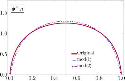
(a)

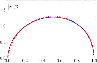
(b)

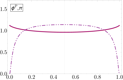
(c)

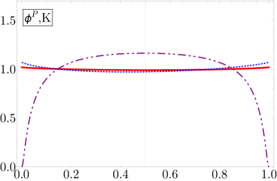
(d)

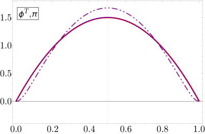
(e)

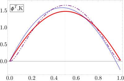
(f)

Figure 6: Unevolved DA, at $Q=Q_{0}=631\,\textrm{MeV}$, with certain modifications to the effective mass. ”Original” (red-thick-solid) denotes (23), (IV.2), and (28). ”mod(1)” (blue-dotted) denotes the shifted effective mass, and ”mod(2)” (purple-dash-dot-dot) the shifted cutoff. See text.

VII.3 Modifications to the Constituent Quark Mass

Our effective quark mass obtained at leading order in $\alpha$ is given by (16). A plot of the zero-momentum limit as a function of current mass $m$ is shown in fig. 2. This constituent quark mass has the interesting property of being approximately constant for $0\,\textrm{MeV}<m<180\,\textrm{MeV}$, assuming phenomenological values of $\rho$ and $\alpha$. Although obtained from a $O(\alpha)$ integral equation, (16) contains higher powers of $\alpha$ resummed into dependence on $m$ through $\xi$. If we maintain strict power counting in $\alpha$ and simultaneously assume sufficiently small quark mass $m$ such that $\xi\ll 1$ (for our parameter values this is not true), then we arrive at the approximation $M(k,m)\approx M(k)+m$. We insert this approximation into the expressions for the DAs and see how they change. In fig. 6, this change is denoted by ”mod(1)”. The most notable resulting change is seen in the kaon pseudotensor DA, which no longer approaches zero at $x\rightarrow 1$. A slight restoration of $x\leftrightarrow\bar{x}$ symmetry is seen in the kaon twist-2 DA. All other DAs are relatively unchanged.

Finally, we consider the effect of restricting $k_{\perp}>M(0,m)$ in the cutoff (35), as was noted in section IV. This modification was implicitly present in our previous paper Kock et al. (2020). In fig. 6 this change is denoted by ”mod(2)”. This results in a slight narrowing of the axial-vector (twist-2) and pseudotensor (twist-3) DAs. The biggest change is seen in the pseudoscalar (twist-3) DA, which becomes concave.

References

- Ji (2013) Xiangdong Ji, “Parton Physics on a Euclidean Lattice,” Phys. Rev. Lett. 110, 262002 (2013), arXiv:1305.1539 [hep-ph] .
- Zhang et al. (2017) Jian-Hui Zhang, Jiunn-Wei Chen, Xiangdong Ji, Luchang Jin, and Huey-Wen Lin, “Pion Distribution Amplitude from Lattice QCD,” Phys. Rev. D 95, 094514 (2017), arXiv:1702.00008 [hep-lat] .
- Ji et al. (2015) Xiangdong Ji, Andreas Schäfer, Xiaonu Xiong, and Jian-Hui Zhang, “One-Loop Matching for Generalized Parton Distributions,” Phys. Rev. D 92, 014039 (2015), arXiv:1506.00248 [hep-ph] .
- Bali et al. (2018) Gunnar S. Bali, Vladimir M. Braun, Benjamin Gläßle, Meinulf Göckeler, Michael Gruber, Fabian Hutzler, Piotr Korcyl, Andreas Schäfer, Philipp Wein, and Jian-Hui Zhang, “Pion distribution amplitude from Euclidean correlation functions: Exploring universality and higher-twist effects,” Phys. Rev. D 98, 094507 (2018), arXiv:1807.06671 [hep-lat] .
- Alexandrou et al. (2018) Constantia Alexandrou, Krzysztof Cichy, Martha Constantinou, Karl Jansen, Aurora Scapellato, and Fernanda Steffens, “Transversity parton distribution functions from lattice QCD,” Phys. Rev. D 98, 091503 (2018), arXiv:1807.00232 [hep-lat] .
- Izubuchi et al. (2019) Taku Izubuchi, Luchang Jin, Christos Kallidonis, Nikhil Karthik, Swagato Mukherjee, Peter Petreczky, Charles Shugert, and Sergey Syritsyn, “Valence parton distribution function of pion from fine lattice,” Phys. Rev. D 100, 034516 (2019), arXiv:1905.06349 [hep-lat] .
- Izubuchi et al. (2018) Taku Izubuchi, Xiangdong Ji, Luchang Jin, Iain W. Stewart, and Yong Zhao, “Factorization Theorem Relating Euclidean and Light-Cone Parton Distributions,” Phys. Rev. D 98, 056004 (2018), arXiv:1801.03917 [hep-ph] .
- Ji et al. (2019) Xiangdong Ji, Yizhuang Liu, and Ismail Zahed, “Quasiparton distribution functions: Two-dimensional scalar and spinor QCD,” Phys. Rev. D 99, 054008 (2019), arXiv:1807.07528 [hep-ph] .
- Briceño et al. (2017) Raúl A. Briceño, Maxwell T. Hansen, and Christopher J. Monahan, “Role of the euclidean signature in lattice calculations of quasidistributions and other nonlocal matrix elements,” Phys. Rev. D 96, 014502 (2017).
- Radyushkin (2017) Anatoly V. Radyushkin, “Pion Distribution Amplitude and Quasi-Distributions,” Phys. Rev. D 95, 056020 (2017), arXiv:1701.02688 [hep-ph] .
- Ma and Qiu (2018) Yan-Qing Ma and Jian-Wei Qiu, “Extracting Parton Distribution Functions from Lattice QCD Calculations,” Phys. Rev. D 98, 074021 (2018), arXiv:1404.6860 [hep-ph] .
- Chu et al. (1994) M.C. Chu, J.M. Grandy, S. Huang, and John W. Negele, “Evidence for the role of instantons in hadron structure from lattice QCD,” Phys. Rev. D 49, 6039–6050 (1994), arXiv:hep-lat/9312071 .
- Diakonov and Petrov (2007) Dmitri Diakonov and Victor Petrov, “Confining ensemble of dyons,” Phys. Rev. D 76, 056001 (2007), arXiv:0704.3181 [hep-th] .
- Liu et al. (2015) Yizhuang Liu, Edward Shuryak, and Ismail Zahed, “Confining dyon-antidyon Coulomb liquid model. I.” Phys. Rev. D 92, 085006 (2015), arXiv:1503.03058 [hep-ph] .
- Greensite (2017) Jeff Greensite, “Confinement from Center Vortices: A review of old and new results,” EPJ Web Conf. 137, 01009 (2017), arXiv:1610.06221 [hep-lat] .
- Biddle et al. (2020) James C. Biddle, Waseem Kamleh, and Derek B. Leinweber, “Visualization of center vortex structure,” Phys. Rev. D 102, 034504 (2020), arXiv:1912.09531 [hep-lat] .
- Kock et al. (2020) Arthur Kock, Yizhuang Liu, and Ismail Zahed, “Pion and kaon parton distributions in the qcd instanton vacuum,” Phys. Rev. D 102, 014039 (2020).
- Nam and Kim (2006) Seung-il Nam and Hyun-Chul Kim, “Twist-3 pion and kaon distribution amplitudes from the instanton vacuum with flavor SU(3) symmetry breaking,” Phys. Rev. D 74, 096007 (2006), arXiv:hep-ph/0608018 .
- Choi and Ji (2017) Ho-Meoyng Choi and Chueng-Ryong Ji, “Twist-3 Distribution Amplitudes of Pion in the Light-Front Quark Model,” Few Body Syst. 58, 31 (2017), arXiv:1611.03201 [hep-ph] .
- Moran and Leinweber (2008) P. J. Moran and D. B. Leinweber, “Buried treasure in the sand of the QCD vacuum,” in QCD Downunder II (2008) arXiv:0805.4246 [hep-lat] .
- Shuryak (1982) Edward V. Shuryak, “The Role of Instantons in Quantum Chromodynamics. 1. Physical Vacuum,” Nucl. Phys. B 203, 93 (1982).
- Schäfer and Shuryak (1998) Thomas Schäfer and Edward V. Shuryak, “Instantons in QCD,” Rev. Mod. Phys. 70, 323–426 (1998), arXiv:hep-ph/9610451 .
- Ji et al. (2020) Xiangdong Ji, Yizhuang Liu, Yu-Sheng Liu, Jian-Hui Zhang, and Yong Zhao, “Large-Momentum Effective Theory,” (2020), arXiv:2004.03543 [hep-ph] .
- Liu and Zahed (2021) Yizhuang Liu and Ismail Zahed, “Small size instanton contributions to the quark quasi-PDF and matching kernel,” (2021), arXiv:2102.07248 [hep-ph] .
- Hasenfratz (2000) Anna Hasenfratz, “Spatial correlation of the topological charge in pure SU(3) gauge theory and in QCD,” Phys. Lett. B 476, 188–192 (2000), arXiv:hep-lat/9912053 .
- Shuryak (1999) Edward V. Shuryak, “Probing the boundary of the nonperturbative QCD by small size instantons,” (1999), arXiv:hep-ph/9909458 .
- Geshkenbein and Terentev (1982) B.V. Geshkenbein and M.V. Terentev, “THE ENHANCED POWER CORRECTION TO THE ASYMPTOTICS OF THE PION FORM-FACTOR,” Phys. Lett. B 117, 243–246 (1982).
- Shuryak and Zahed (2020) Edward Shuryak and Ismail Zahed, “Nonperturbative quark-antiquark interactions in mesonic form factors,” (2020), arXiv:2008.06169 [hep-ph] .
- Bowman et al. (2004) Patrick O. Bowman, Urs M. Heller, Derek B. Leinweber, Anthony G. Williams, and Jianbo Zhang, “Infrared and ultraviolet properties of the landau gauge quark propagator,” Nuclear Physics B - Proceedings Supplements 128, 23–29 (2004), proceedings of the 2nd Cairns Topical Workshop on Lattice Hadron Physics.
- Broniowski and Ruiz Arriola (2017) Wojciech Broniowski and Enrique Ruiz Arriola, “Nonperturbative partonic quasidistributions of the pion from chiral quark models,” Phys. Lett. B 773, 385–390 (2017), arXiv:1707.09588 [hep-ph] .
- Jia and Vary (2019) Shaoyang Jia and James P. Vary, “Basis light front quantization for the charged light mesons with color singlet Nambu–Jona-Lasinio interactions,” Phys. Rev. C 99, 035206 (2019), arXiv:1811.08512 [nucl-th] .
- Ding et al. (2020) Minghui Ding, Khépani Raya, Daniele Binosi, Lei Chang, Craig D. Roberts, and Sebastian M. Schmidt, “Symmetry, symmetry breaking, and pion parton distributions,” Phys. Rev. D 101, 054014 (2020).
- Shifman and Vysotsky (1981) M. Shifman and M. Vysotsky, “Form factors of heavy mesons in qcd,” Nuclear Physics 186, 475–518 (1981).
- de Melo et al. (2016) J. P. B. C. de Melo, Isthiaq Ahmed, and Kazuo Tsushima, “Parton distribution in pseudoscalar mesons with a light-front constituent quark model,” AIP Conference Proceedings 1735, 080012 (2016), https://aip.scitation.org/doi/pdf/10.1063/1.4949465 .
- Zhang et al. (2020) Rui Zhang, Carson Honkala, Huey-Wen Lin, and Jiunn-Wei Chen, “Pion and kaon distribution amplitudes in the continuum limit,” Phys. Rev. D 102, 094519 (2020).
- Shi et al. (2015) Chao Shi, Chen Chen, Lei Chang, Craig D. Roberts, Sebastian M. Schmidt, and Hong-Shi Zong, “Kaon and pion parton distribution amplitudes to twist three,” Phys. Rev. D 92, 014035 (2015).
- Aitala (2001) E. M. et al. Aitala (Fermilab E791 Collaboration), “Direct measurement of the pion valence-quark momentum distribution, the pion light-cone wave function squared,” Phys. Rev. Lett. 86, 4768–4772 (2001).
- Zahed (2021) Ismail Zahed, “Mass sum rule of hadrons in the QCD instanton vacuum,” (2021), arXiv:2102.08191 [hep-ph] .